


1. Introduction
The plume theory developed by Morton, Taylor & Turner (Reference Morton, Taylor and Turner1956), hereafter referred to as the MTT56 model, provides an elegant and simple means of describing the complex effects of turbulence in jets and plumes. The success of their approach can be attributed to the fact that such flows have a natural tendency to evolve spatially in a state of self-similarity (Tollmien Reference Tollmien1926; George Reference George, George and Arndt1989), such that the evolution of a single characteristic length, velocity and buoyancy scale suffice for obtaining predictions of their integral quantities. In the event that such strict similarity is not attained in higher-order statistics of the flow, predictive models based on the similarity of lower-order quantities often remain useful, even in stratified environments (Morton Reference Morton1971). For a review of the wide variety of applications that exist for plume theory the reader is referred to Woods (Reference Woods2010).
The classical plume theory, describing the behaviour of statistically steady jets and plumes, has subsequently been extended to unsteady cases. Indeed, such processes prevail in many natural and man-made situations: the accidental release of contaminant, the melting of ice sheets, volcanic eruptions and natural ventilation are inherently ‘unsteady’ problems. The first extension of classical plume theory to unsteady plumes appears to be that of Turner (Reference Turner1962) with a model of a ‘starting plume’, which combined the motion of a front with that of a steady plume beneath. Motivated by the need to predict the response of fire detectors, subsequent work focused on the buoyant plumes occurring above growing fires (see e.g. Delichatsios Reference Delichatsios1979; Heskestad Reference Heskestad1998). As such, much attention was paid to time similarity solutions in which all variables are rescaled by the scales appearing at the leading edge of a front. Delichatsios (Reference Delichatsios1979) showed that such similarity solutions require a power-law dependence of the source buoyancy flux on time and coincide with a quasi-steady approximation close to the source. Despite the fact that they are all based on the same physical conservation laws, namely mass, momentum and buoyancy, amongst these early unsteady plume models and those developed subsequently by Yu (Reference Yu1990), Vul’fson & Borodin (Reference Vul’fson and Borodin2001) and Scase et al. (Reference Scase, Caulfield, Dalziel and Hunt2006), one finds significant differences. In particular, each model invokes a particular assumption regarding the radial dependence of the mean longitudinal velocity profile, which, as Scase & Hewitt (Reference Scase and Hewitt2012) point out, can lead to difficulties in the derivation of an integral mass conservation equation.
It was recently discovered that the unsteady plume models of Delichatsios (Reference Delichatsios1979), Yu (Reference Yu1990) and Scase et al. (Reference Scase, Caulfield, Dalziel and Hunt2006) are ill-posed (Scase & Hewitt Reference Scase and Hewitt2012), because they do not account for longitudinal mixing processes. Indeed, their governing integral equations are consistent with the view that lateral slices of the jet or plume do not interact longitudinally (Scase, Aspden & Caulfield Reference Scase, Aspden and Caulfield2009). However, possible sources of longitudinal mixing such as turbulence and lateral gradients of mean velocity (causing dispersion) are evident in numerous experimental studies of steady jets and plumes (e.g. Kotsovinos & List Reference Kotsovinos and List1977; Panchapakesan & Lumley Reference Panchapakesan and Lumley1993). Moreover, Landel, Caulfield & Woods (Reference Landel, Caulfield and Woods2012) recently found that in the unsteady transport of a passive tracer in a quasi-two-dimensional steady jet, the role of dispersion arising from non-uniform velocity profiles was non-negligible, compared to the idealised ‘top-hat’ jet, from which dispersion is absent. For three-dimensional unsteady jets and plumes the physical processes responsible for longitudinal mixing, and therefore their faithful representation in models, are not currently understood and necessitate the use of an ad hoc closure (Scase & Hewitt Reference Scase and Hewitt2012). Similarly, the effect that turbulence mixing and radial profiles have on the propagation speed and growth of disturbances in unsteady jets and plumes is not known.
A contribution to experimental data pertaining to unsteady plumes was made by Scase, Caulfield & Dalziel (Reference Scase, Caulfield and Dalziel2008), who investigated the effects of a sudden reduction in buoyancy flux. In particular, Scase et al. (Reference Scase, Caulfield and Dalziel2008) found that source conditions that maintain turbulence in the plume cannot be changed so as to disconnect the plume into individual thermals, a finding which adds validity to the description of such flows using plume theory. Nevertheless, experimental data for unsteady plumes remain limited, which is partly due to the difficulty of obtaining many realisations of an ‘identical’ experiment (Scase et al. Reference Scase, Caulfield, Dalziel and Hunt2006). In the context of flow control, several experimental studies of unsteady jets have investigated the enhanced entrainment that is caused by periodic excitation of the flow (see e.g. Bremhorst & Hollis Reference Bremhorst and Hollis1990, and references therein). Similarly, Borée et al. (Reference Borée, Atassi, Charnay and Taubert1997) observed a relatively large radial inflow in the vicinity of a rapid reduction in the velocity of an unsteady jet.
For the ease with which statistics can be taken over homogeneous dimensions, numerical simulations offer a significant advantage over experiments. In addition, numerical simulations allow one to control the source conditions arbitrarily and therefore investigate a broad range of problems or, alternatively, a canonical case that is difficult to realise in a laboratory. In Scase et al. (Reference Scase, Aspden and Caulfield2009) the unsteady plume theory of Scase et al. (Reference Scase, Caulfield, Dalziel and Hunt2006) was able to successfully predict the scaling of a ‘pulse’ in the plume’s radius that was observed in implicit large-eddy simulations of a plume, whose buoyancy flux was suddenly increased. However, the observed longitudinal scaling of the pulse and effects relating to longitudinal mixing were not predicted by the theoretical model and these remain issues warranting further attention.
Our aim is to establish the physical processes responsible for longitudinal mixing so that their effects can be accurately represented in simple and robust integral models. We examine pure momentum jets, rather than plumes, in order to focus exclusively on the behaviour of the volume flux and momentum flux. Central to our approach is the fact that we derive the governing integral equations for unsteady jets from first principles, without invoking any assumptions about self-similarity, the form of radial dependence or the magnitude of turbulent transport terms. This allows us to examine the behaviour of both steady and unsteady jets from a integral perspective comprehensively, and therefore address the validity of some of the assumptions that are used in existing unsteady plume models. We do this by using the formalism of Priestley & Ball (Reference Priestley and Ball1955, hereafter referred to as PB55), who obtain a complete system of equations for plumes by integrating a mean kinetic energy equation, derived from mass conservation and momentum conservation, rather than integrating the mass conservation equation directly. This approach was used recently by Kaminski, Tait & Carazzo (Reference Kaminski, Tait and Carazzo2005, hereafter referred to as KTC05) to investigate a decomposition of the entrainment coefficient for steady plumes. Subsequently, Carazzo, Kaminski & Tait (Reference Carazzo, Kaminski and Tait2006) applied the approach in the systematic analysis of self-similarity in jets and plumes from a wide variety of experimental results. Here we will show that the energy equation can be used to obtain an unsteady area or mass conservation equation for unsteady jets at the integral level, which generalises the equations used in existing models to arbitrary profiles that are not restricted to remain self-similar.
The work is split into two parts. In this part of the work we use our framework in a diagnostic capacity to analyse results from the direct numerical simulation (DNS) of steady and unsteady jets. In Part 2 (Craske & van Reeuwijk Reference Craske and van Reeuwijk2015), we employ our framework as a prognostic tool and develop a dispersion closure for unsteady jets. In addition, we demonstrate the role that dispersion plays in determining the behaviour of the area of the jet and the response of integral fluxes to source perturbations. The present paper is organised as follows. In § 2 we develop the framework by deriving a system of governing integral equations for unsteady jets that describe the conservation of mass, momentum and energy. Simulation details are provided in § 3, and in § 4 we present results from the simulation of steady and unsteady jets. In particular, in § 4.3 we determine the propagation velocity of the front appearing in the unsteady jets, and show that its evolution is a self-similar process. In § 5 we develop theory applicable to the front, relating the observations of § 4.3 to two types of dispersion, before drawing conclusions in § 6.
2. The governing equations
In this section we derive the equations governing the motion of an unsteady jet. In doing so, we move from the Navier–Stokes equations to a much simpler system of equations that determine the behaviour of integral quantities in the jet. The two main differences between our approach and the approach adopted by the plume theory of MTT56 is that (i) we retain higher-order terms that are typically neglected, and (ii) following PB55 and KTC05 we supplement the classical mass–momentum formulation with a conservation equation for energy. We then demonstrate that a mass conservation equation can be derived from the momentum–energy pair, which gives unknown parameters appearing in the former an alternative and more direct physical interpretation. The momentum–energy formulation will prove to be an elucidating framework in the analysis of the unsteady problem undertaken in §§ 4.3 and 5.
2.1. Reynolds equations
Consider a round, turbulent jet orientated in the longitudinal (
 $z$
) direction whose flow is statistically axisymmetric and swirl-free. Since the mean motion in the jet is in the longitudinal direction we only need to consider the continuity equation and longitudinal momentum equation, which in cylindrical coordinates are
$z$
) direction whose flow is statistically axisymmetric and swirl-free. Since the mean motion in the jet is in the longitudinal direction we only need to consider the continuity equation and longitudinal momentum equation, which in cylindrical coordinates are
 $$\begin{eqnarray}\displaystyle & \displaystyle \frac{1}{r}\frac{\partial (ru)}{\partial r}+\frac{1}{r}\frac{\partial v}{\partial {\it\phi}}+\frac{\partial w}{\partial z}=0, & \displaystyle\end{eqnarray}$$
 $$\begin{eqnarray}\displaystyle & \displaystyle \frac{\partial w}{\partial t}+u\frac{\partial w}{\partial r}+\frac{v}{r}\frac{\partial w}{\partial {\it\phi}}+w\frac{\partial w}{\partial z}=-\frac{\partial p}{\partial z}+{\it\nu}{\rm\nabla}^{2}w. & \displaystyle\end{eqnarray}$$
 $(u,v,w)$
correspond to the directions
$(u,v,w)$
correspond to the directions
 $(r,{\it\phi},z)$
, respectively;
$(r,{\it\phi},z)$
, respectively;
 $p$
denotes kinematic pressure and
$p$
denotes kinematic pressure and
 ${\it\nu}$
is the kinematic viscosity. The hydrostatic balance
${\it\nu}$
is the kinematic viscosity. The hydrostatic balance
 $\partial _{z}\,p_{h}=-g$
has been subtracted, so that
$\partial _{z}\,p_{h}=-g$
has been subtracted, so that
 $p$
is constant in a quiescent environment. Hereafter we shall denote by
$p$
is constant in a quiescent environment. Hereafter we shall denote by
 $\overline{{\it\chi}}$
the ensemble average of a variable
$\overline{{\it\chi}}$
the ensemble average of a variable
 ${\it\chi}$
, so that
${\it\chi}$
, so that
 ${\it\chi}\equiv \overline{{\it\chi}}+{\it\chi}^{\prime }$
, where
${\it\chi}\equiv \overline{{\it\chi}}+{\it\chi}^{\prime }$
, where
 $\overline{{\it\chi}^{\prime }}=0$
. In the current problem the statistical axisymmetry of jets above axisymmetric sources ensures that
$\overline{{\it\chi}^{\prime }}=0$
. In the current problem the statistical axisymmetry of jets above axisymmetric sources ensures that
 $\partial _{{\it\phi}}=0$
. Taking an ensemble average of (2.1) and (2.2) yields
$\partial _{{\it\phi}}=0$
. Taking an ensemble average of (2.1) and (2.2) yields  $$\begin{eqnarray}\displaystyle & \displaystyle \frac{1}{r}\frac{\partial (r\overline{u})}{\partial r}+\frac{\partial \overline{w}}{\partial z}=0, & \displaystyle\end{eqnarray}$$
 $$\begin{eqnarray}\displaystyle & \displaystyle \frac{\partial \overline{w}}{\partial t}+\frac{1}{r}\frac{\partial (r\overline{u}\,\overline{w})}{\partial r}+\frac{\partial \overline{w}^{2}}{\partial z}+\frac{1}{r}\frac{\partial (r\overline{u^{\prime }w^{\prime }})}{\partial r}+\frac{\partial \overline{w^{\prime 2}}}{\partial z}=-\frac{\partial \overline{p}}{\partial z}+{\it\nu}{\rm\nabla}^{2}\overline{w}. & \displaystyle\end{eqnarray}$$
 $2\overline{w}$
and utilising (2.3):
$2\overline{w}$
and utilising (2.3):  $$\begin{eqnarray}\displaystyle & & \displaystyle \frac{\partial \overline{w}^{2}}{\partial t}+\frac{1}{r}\frac{\partial (r\overline{u}\,\overline{w}^{2})}{\partial r}+\frac{\partial \overline{w}^{3}}{\partial z}+2\frac{\partial (\overline{p}\,\overline{w})}{\partial z}+\frac{2}{r}\frac{\partial (r\overline{u^{\prime }w^{\prime }}\overline{w})}{\partial r}+2\,\frac{\partial (\overline{w^{\prime 2}}\overline{w})}{\partial z}\nonumber\\ \displaystyle & & \displaystyle \quad =2\overline{p}\frac{\partial \overline{w}}{\partial z}+2\,\overline{w^{\prime 2}}\frac{\partial \overline{w}}{\partial z}+2\,\overline{u^{\prime }w^{\prime }}\frac{\partial \overline{w}}{\partial r}+{\it\nu}{\rm\nabla}^{2}\overline{w}^{2}-2{\it\nu}\left(\frac{\partial \overline{w}}{\partial r}\right)^{2}-2{\it\nu}\left(\frac{\partial \overline{w}}{\partial z}\right)^{2}.\end{eqnarray}$$
To assess the magnitude of the viscous terms we consider a longitudinal velocity scale,
 $w_{m}$
, a velocity scale for the turbulence,
$w_{m}$
, a velocity scale for the turbulence,
 $w_{f}$
, a radial length scale
$w_{f}$
, a radial length scale
 $r_{m}$
and a longitudinal length scale
$r_{m}$
and a longitudinal length scale
 $L$
. A local Reynolds number can be defined using these integral scales:
$L$
. A local Reynolds number can be defined using these integral scales:
 $\mathit{Re}_{f}\equiv w_{f}r_{m}/{\it\nu}$
. In classical plume theory it is assumed that
$\mathit{Re}_{f}\equiv w_{f}r_{m}/{\it\nu}$
. In classical plume theory it is assumed that
 $\mathit{Re}_{f}\rightarrow \infty$
and
$\mathit{Re}_{f}\rightarrow \infty$
and
 $r_{m}/L\rightarrow 0$
, which implies that
$r_{m}/L\rightarrow 0$
, which implies that
 $w_{f}/w_{m}\sim (r_{m}/L)^{1/2}$
(see e.g. Tennekes & Lumley Reference Tennekes and Lumley1972, for details). In this limit it is necessary that
$w_{f}/w_{m}\sim (r_{m}/L)^{1/2}$
(see e.g. Tennekes & Lumley Reference Tennekes and Lumley1972, for details). In this limit it is necessary that
 $\mathit{Re}_{f}\gg (L/r_{m})^{1/2}$
in order that the viscous terms are negligible in both the mean momentum and mean kinetic energy equation. In contrast to steady problems, in unsteady problems there is no guarantee that
$\mathit{Re}_{f}\gg (L/r_{m})^{1/2}$
in order that the viscous terms are negligible in both the mean momentum and mean kinetic energy equation. In contrast to steady problems, in unsteady problems there is no guarantee that
 $r_{m}/L\ll 1$
, owing to the possibility of sudden changes in the longitudinal direction. Thus, we take the limit
$r_{m}/L\ll 1$
, owing to the possibility of sudden changes in the longitudinal direction. Thus, we take the limit
 $\mathit{Re}_{f}\rightarrow \infty$
independently and retain terms that are
$\mathit{Re}_{f}\rightarrow \infty$
independently and retain terms that are
 $O(r_{m}/L)$
relative to the leading-order balance:
$O(r_{m}/L)$
relative to the leading-order balance:
 $$\begin{eqnarray}\frac{\partial \overline{w}}{\partial t}+\frac{1}{r}\frac{\partial (r\overline{u}\,\overline{w})}{\partial r}+\frac{\partial \overline{w}^{2}}{\partial z}+\frac{1}{r}\frac{\partial (r\overline{u^{\prime }w^{\prime }})}{\partial r}+\underbrace{\frac{\partial \overline{w^{\prime 2}}}{\partial z}}_{O\left(r_{m}/L\right)}=\underbrace{-\frac{\partial \overline{p}}{\partial z}}_{O\left(r_{m}/L\right)},\end{eqnarray}$$
describing the mean longitudinal momentum, and
 $$\begin{eqnarray}\displaystyle & & \displaystyle \frac{\partial \overline{w}^{2}}{\partial t}+\frac{1}{r}\frac{\partial (r\overline{u}\,\overline{w}^{2})}{\partial r}+\frac{\partial \overline{w}^{3}}{\partial z}+\overbrace{2\frac{\partial (\,\overline{p}\,\overline{w})}{\partial z}+2\,\frac{\partial (\overline{w^{\prime 2}}\overline{w})}{\partial z}}^{O\left(r_{m}/L\right)}+\,\frac{2}{r}\frac{\partial (r\overline{u^{\prime }w^{\prime }}\overline{w})}{\partial r}\nonumber\\ \displaystyle & & \displaystyle \quad =\underbrace{2\overline{p}\frac{\partial \overline{w}}{\partial z}+2\,\overline{w^{\prime 2}}\frac{\partial \overline{w}}{\partial z}}_{O\left(r_{m}/L\right)}+\,2\,\overline{u^{\prime }w^{\prime }}\frac{\partial \overline{w}}{\partial r},\end{eqnarray}$$
describing the mean longitudinal kinetic energy. Here we note that for steady jets, their slenderness
 $r_{m}/L\sim 2{\it\alpha}\approx 0.2$
, where
$r_{m}/L\sim 2{\it\alpha}\approx 0.2$
, where
 ${\it\alpha}$
is the classical entrainment coefficient, so that the assumption
${\it\alpha}$
is the classical entrainment coefficient, so that the assumption
 $r_{m}/L\ll 1$
is questionable even for steady jets. Collectively, the terms on the right-hand side of (2.7) represent a sink for the kinetic energy carried by the mean longitudinal flow, acting either to redistribute the energy to the other mean flow components or to produce turbulence kinetic energy. In §§ 2.4–2.5 we show that entrainment can be viewed as a consequence of this energy sink. In general the jet does work on its surrounding fluid, redistributing its momentum flux over an area that increases, at the expense of a longitudinally diminishing flux of kinetic energy. It should be noted that in the system (2.3), (2.6) and (2.7), there exist only two independent equations, because the equation for kinetic energy is a mechanical equation that was obtained using the continuity and momentum conservation equations. The aspect of these equations that is most pertinent to the present study is the fact that
$r_{m}/L\ll 1$
is questionable even for steady jets. Collectively, the terms on the right-hand side of (2.7) represent a sink for the kinetic energy carried by the mean longitudinal flow, acting either to redistribute the energy to the other mean flow components or to produce turbulence kinetic energy. In §§ 2.4–2.5 we show that entrainment can be viewed as a consequence of this energy sink. In general the jet does work on its surrounding fluid, redistributing its momentum flux over an area that increases, at the expense of a longitudinally diminishing flux of kinetic energy. It should be noted that in the system (2.3), (2.6) and (2.7), there exist only two independent equations, because the equation for kinetic energy is a mechanical equation that was obtained using the continuity and momentum conservation equations. The aspect of these equations that is most pertinent to the present study is the fact that
 $\overline{w}$
,
$\overline{w}$
,
 $w^{\prime }$
, etc. have an a priori unknown dependence on
$w^{\prime }$
, etc. have an a priori unknown dependence on
 $r$
, which is manifested as profile constants when the equations are integrated.
$r$
, which is manifested as profile constants when the equations are integrated.
2.2. Integral equations
In an axisymmetric jet the primary variables of interest are the longitudinal volume flux and the longitudinal specific momentum flux (hereafter referred to as the momentum flux for brevity), defined as
 $Q_{m}$
and
$Q_{m}$
and
 $M_{m}$
, respectively, where
$M_{m}$
, respectively, where
 $$\begin{eqnarray}Q_{m}\equiv 2\int _{0}^{r_{d}(z,t)}\overline{w}r\text{d}r,\quad M_{m}\equiv 2\int _{0}^{r_{d}(z,t)}\overline{w}^{2}r\text{d}r.\end{eqnarray}$$
Here we have used the subscript
 $m$
to denote the fact that these quantities are based on the integrals of a mean value. In this work the upper limit of integration
$m$
to denote the fact that these quantities are based on the integrals of a mean value. In this work the upper limit of integration
 $r_{d}$
, used to define all integral quantities, is defined to be the smallest value of
$r_{d}$
, used to define all integral quantities, is defined to be the smallest value of
 $r$
at which longitudinal velocities are relatively small:
$r$
at which longitudinal velocities are relatively small:
 $$\begin{eqnarray}\overline{w}(r_{d},z,t)={\it\epsilon}\overline{w}(0,z,t),\end{eqnarray}$$
where the small parameter
 ${\it\epsilon}\ll 1$
ensures that longitudinal fluxes of volume and momentum across the boundary of the jet are relatively insignificant. Indeed, when the improper integral for
${\it\epsilon}\ll 1$
ensures that longitudinal fluxes of volume and momentum across the boundary of the jet are relatively insignificant. Indeed, when the improper integral for
 $r_{d}\rightarrow \infty$
is used the resulting definitions of
$r_{d}\rightarrow \infty$
is used the resulting definitions of
 $Q_{m}$
and
$Q_{m}$
and
 $M_{m}$
will, in general, depend on the precise way in which the induced ambient flow is bounded (Kotsovinos Reference Kotsovinos1978). By defining integral quantities in terms of
$M_{m}$
will, in general, depend on the precise way in which the induced ambient flow is bounded (Kotsovinos Reference Kotsovinos1978). By defining integral quantities in terms of
 $r_{d}$
(see also the approach employed by Kotsovinos & List Reference Kotsovinos and List1977), we focus attention on the dynamics of the jet. In this study we do not address the dynamics of the flow that is induced in the ambient. For a resolution of the related issue of how a given velocity profile, not necessarily possessing compact support, can be reconciled with the MTT56 framework, the reader is referred to Scase et al. (Reference Scase, Caulfield, Linden and Dalziel2007).
$r_{d}$
(see also the approach employed by Kotsovinos & List Reference Kotsovinos and List1977), we focus attention on the dynamics of the jet. In this study we do not address the dynamics of the flow that is induced in the ambient. For a resolution of the related issue of how a given velocity profile, not necessarily possessing compact support, can be reconciled with the MTT56 framework, the reader is referred to Scase et al. (Reference Scase, Caulfield, Linden and Dalziel2007).
From the definitions of
 $Q_{m}$
and
$Q_{m}$
and
 $M_{m}$
naturally follow characteristic length and velocity scales:
$M_{m}$
naturally follow characteristic length and velocity scales:
 $$\begin{eqnarray}r_{m}\equiv \frac{Q_{m}}{M_{m}^{1/2}},\quad w_{m}\equiv \frac{M_{m}}{Q_{m}},\end{eqnarray}$$
which are consistent with a top-hat interpretation of the radial profiles such that
 $Q_{m}\equiv w_{m}r_{m}^{2}$
and
$Q_{m}\equiv w_{m}r_{m}^{2}$
and
 $M_{m}\equiv w_{m}^{2}r_{m}^{2}$
, although here we make no assumptions regarding radial dependence. Additionally, we define a characteristic area for the jet,
$M_{m}\equiv w_{m}^{2}r_{m}^{2}$
, although here we make no assumptions regarding radial dependence. Additionally, we define a characteristic area for the jet,
 $A_{m}\equiv r_{m}^{2}$
. Although a transport equation for the area
$A_{m}\equiv r_{m}^{2}$
. Although a transport equation for the area
 $A_{m}$
can be obtained directly using mass conservation and applying an appropriate kinematic boundary condition, this procedure is not straightforward and requires that stringent assumptions are made about the velocity profile (see e.g. Scase et al.
Reference Scase, Caulfield, Dalziel and Hunt2006). The difficulty in obtaining a canonical transport equation for
$A_{m}$
can be obtained directly using mass conservation and applying an appropriate kinematic boundary condition, this procedure is not straightforward and requires that stringent assumptions are made about the velocity profile (see e.g. Scase et al.
Reference Scase, Caulfield, Dalziel and Hunt2006). The difficulty in obtaining a canonical transport equation for
 $A_{m}$
is reflected in the variety of slightly different equations that have been adopted in unsteady plume models (compare, for example, Delichatsios Reference Delichatsios1979; Yu Reference Yu1990). Nevertheless, a generic equation for
$A_{m}$
is reflected in the variety of slightly different equations that have been adopted in unsteady plume models (compare, for example, Delichatsios Reference Delichatsios1979; Yu Reference Yu1990). Nevertheless, a generic equation for
 $A_{m}$
that encompasses these different approaches is
$A_{m}$
that encompasses these different approaches is
 $$\begin{eqnarray}\frac{1}{{\it\gamma}_{g}}\frac{\partial A_{m}}{\partial t}+\frac{\partial Q_{m}}{\partial z}=2{\it\alpha}M_{m}^{1/2},\end{eqnarray}$$
where
 ${\it\alpha}$
is the classical entrainment coefficient used by MTT56 and
${\it\alpha}$
is the classical entrainment coefficient used by MTT56 and
 $1/{\it\gamma}_{g}$
is a free parameter. By looking at integral transport equations for the volume flux and the momentum flux, we will reveal the physical meaning of
$1/{\it\gamma}_{g}$
is a free parameter. By looking at integral transport equations for the volume flux and the momentum flux, we will reveal the physical meaning of
 ${\it\gamma}_{g}$
and obtain an explicit expression for
${\it\gamma}_{g}$
and obtain an explicit expression for
 ${\it\alpha}$
.
${\it\alpha}$
.
Integration of (2.6) and (2.7), over a horizontal disk of radius
 $r_{d}(z,t)$
, and dividing by
$r_{d}(z,t)$
, and dividing by
 ${\rm\pi}$
results in integral conservation equations for momentum and energy:
${\rm\pi}$
results in integral conservation equations for momentum and energy:
 $$\begin{eqnarray}\displaystyle & \displaystyle \frac{\partial Q_{m}}{\partial t}+\frac{\partial ({\it\beta}_{g}M_{m})}{\partial z}=0, & \displaystyle\end{eqnarray}$$
 $$\begin{eqnarray}\displaystyle & \displaystyle \frac{\partial M_{m}}{\partial t}+\frac{\partial }{\partial z}\left({\it\gamma}_{g}\frac{M_{m}^{2}}{Q_{m}}\right)={\it\delta}_{g}\frac{M_{m}^{5/2}}{Q_{m}^{2}}. & \displaystyle\end{eqnarray}$$
 $Q_{m}$
and
$Q_{m}$
and
 $M_{m}$
as integrals of momentum and energy, respectively, rather than fluxes. A similar equivalence between volume flux and the integral of (specific) momentum is found in the shallow-water equations. To obtain (2.12) and (2.13), we neglect momentum and energy transport on the boundary of the jet, where
$M_{m}$
as integrals of momentum and energy, respectively, rather than fluxes. A similar equivalence between volume flux and the integral of (specific) momentum is found in the shallow-water equations. To obtain (2.12) and (2.13), we neglect momentum and energy transport on the boundary of the jet, where
 $r=r_{d}$
, which is justified for a slender jet provided that
$r=r_{d}$
, which is justified for a slender jet provided that
 ${\it\epsilon}\ll 1$
in (2.9). Indeed, defining the boundary of the jet in terms of
${\it\epsilon}\ll 1$
in (2.9). Indeed, defining the boundary of the jet in terms of
 ${\it\epsilon}$
means that the effects of non-lateral entrainment can be quantified as
${\it\epsilon}$
means that the effects of non-lateral entrainment can be quantified as
 $O({\it\epsilon}^{2})$
and
$O({\it\epsilon}^{2})$
and
 $O({\it\epsilon}^{3})$
terms in the momentum (2.12) and energy (2.13) equations, respectively. In addition, (2.12) and (2.13) do not include a contribution from temporal changes in
$O({\it\epsilon}^{3})$
terms in the momentum (2.12) and energy (2.13) equations, respectively. In addition, (2.12) and (2.13) do not include a contribution from temporal changes in
 $r_{d}$
.
$r_{d}$
.
In the system of equations (2.12) and (2.13)
 ${\it\beta}_{g},{\it\gamma}_{g}$
and
${\it\beta}_{g},{\it\gamma}_{g}$
and
 ${\it\delta}_{g}$
are dimensionless parameters, or profile constants, defined as
${\it\delta}_{g}$
are dimensionless parameters, or profile constants, defined as
 $$\begin{eqnarray}{\it\beta}_{g}\equiv \frac{M_{g}}{M_{m}},\quad {\it\gamma}_{g}\equiv \frac{E_{g}Q_{m}}{M_{m}^{2}},\quad {\it\delta}_{g}\equiv \frac{P_{g}Q_{m}^{2}}{M_{m}^{5/2}},\end{eqnarray}$$
which represent a dimensionless momentum flux, a dimensionless energy flux and a dimensionless turbulence production, respectively. In § 2.4 we will demonstrate that the
 ${\it\gamma}_{g}$
defined above is indeed equal to the
${\it\gamma}_{g}$
defined above is indeed equal to the
 ${\it\gamma}_{g}$
appearing in the area equation (2.11). The dimensionless parameters allow all unknown integrals in the system to be related to
${\it\gamma}_{g}$
appearing in the area equation (2.11). The dimensionless parameters allow all unknown integrals in the system to be related to
 $Q_{m}$
and
$Q_{m}$
and
 $M_{m}$
, which are the dependent variables. We will refer to the quantity
$M_{m}$
, which are the dependent variables. We will refer to the quantity
 $$\begin{eqnarray}M_{g}\equiv \underbrace{2\int _{0}^{r_{d}(z,t)}\overline{w}^{2}r\text{d}r}_{M_{m}}+\underbrace{2\int _{0}^{r_{d}(z,t)}\overline{w^{\prime 2}}r\text{d}r}_{M_{f}}+\underbrace{2\int _{0}^{r_{d}(z,t)}(\overline{p}-p_{d})r\text{d}r}_{M_{p}},\end{eqnarray}$$
as the gross momentum flux, comprising integrals of the mean transport of longitudinal momentum
 $M_{m}$
, the turbulent transport of longitudinal momentum
$M_{m}$
, the turbulent transport of longitudinal momentum
 $M_{f}$
and pressure
$M_{f}$
and pressure
 $M_{p}$
. Here,
$M_{p}$
. Here,
 $p_{d}$
is the pressure in the ambient:
$p_{d}$
is the pressure in the ambient:
 $p_{d}=p(r_{d},z)$
. Similarly, the gross energy flux
$p_{d}=p(r_{d},z)$
. Similarly, the gross energy flux
 $$\begin{eqnarray}E_{g}\equiv \underbrace{2\int _{0}^{r_{d}(z,t)}\overline{w}^{3}r\text{d}r}_{E_{m}}+\underbrace{4\int _{0}^{r_{d}(z,t)}\overline{w}\overline{w^{\prime 2}}r\text{d}r}_{E_{f}}+\underbrace{4\int _{0}^{r_{d}(z,t)}(\overline{p}-p_{d})\overline{w}r\text{d}r}_{E_{p}},\end{eqnarray}$$
includes contributions from the mean flow, in addition to those from turbulence and pressure. The gross turbulence production is defined to include pressure redistribution:
 $$\begin{eqnarray}P_{g}\equiv \underbrace{4\int _{0}^{r_{d}(z,t)}\overline{u^{\prime }w^{\prime }}\frac{\partial \overline{w}}{\partial r}r\text{d}r}_{P_{m}}+\underbrace{4\int _{0}^{r_{d}(z,t)}\overline{w^{\prime 2}}\frac{\partial \overline{w}}{\partial z}r\text{d}r}_{P_{f}}+\underbrace{4\int _{0}^{r_{d}(z,t)}\overline{p}\frac{\partial \overline{w}}{\partial z}r\text{d}r}_{P_{p}}.\end{eqnarray}$$
We will use subscripts in the dimensionless quantities that are consistent with the definitions above, e.g.
 $$\begin{eqnarray}{\it\gamma}_{m}\equiv \frac{E_{m}Q_{m}}{M_{m}^{2}},\quad {\it\gamma}_{f}\equiv \frac{E_{f}Q_{m}}{M_{m}^{2}}\end{eqnarray}$$
represent the dimensionless mean energy flux and dimensionless turbulent energy flux, respectively. The system (2.11)–(2.13) is a generalisation of the approaches adopted by PB55 and MTT56 in the absence of buoyancy. Whilst MTT56 focus on volume and mean momentum conservation using (2.11) and (2.12), PB55 invoke mean momentum and mean energy conservation using (2.12) and (2.13). Central to the current work is the fact, noted by PB55, that only when a particular radial dependence of quantities such as
 $\overline{w}$
and
$\overline{w}$
and
 $\overline{w^{\prime 2}}$
is assumed (e.g. Gaussian), can parameters such as
$\overline{w^{\prime 2}}$
is assumed (e.g. Gaussian), can parameters such as
 ${\it\gamma}_{m}$
and
${\it\gamma}_{m}$
and
 ${\it\gamma}_{f}$
be determined. In particular,
${\it\gamma}_{f}$
be determined. In particular,
 ${\it\gamma}_{m}\geqslant 1$
in general, where equality holds only when the longitudinal velocity is assumed to be distributed uniformly. In a leading-order analysis of the steady state, in which the mean energy equation (2.13) reduces to a balance between two terms, the value of
${\it\gamma}_{m}\geqslant 1$
in general, where equality holds only when the longitudinal velocity is assumed to be distributed uniformly. In a leading-order analysis of the steady state, in which the mean energy equation (2.13) reduces to a balance between two terms, the value of
 ${\it\gamma}_{m}$
has received little attention. This is because, provided that it remains constant,
${\it\gamma}_{m}$
has received little attention. This is because, provided that it remains constant,
 ${\it\gamma}_{m}$
does not affect the steady-state solution independently. Indeed, in such circumstances
${\it\gamma}_{m}$
does not affect the steady-state solution independently. Indeed, in such circumstances
 ${\it\gamma}_{m}$
only enters the problem via the ratio
${\it\gamma}_{m}$
only enters the problem via the ratio
 ${\it\delta}_{m}/{\it\gamma}_{m}$
(see e.g. (2.24) below). However, with the addition of temporal derivatives,
${\it\delta}_{m}/{\it\gamma}_{m}$
(see e.g. (2.24) below). However, with the addition of temporal derivatives,
 ${\it\gamma}_{m}$
plays an independent role in the governing equations.
${\it\gamma}_{m}$
plays an independent role in the governing equations.
2.3. Dispersion and non-uniform velocity profiles
The fact that the radial distribution of velocity in real jets is non-uniform implies that there exists a means of spreading regions of the flow over the longitudinal dimension. Indeed, parcels of fluid located on the jet centreline travel faster than those that are located on its periphery. In this work we will refer to all effects arising from non-uniform velocity profiles as dispersive. However, a further distinction is necessary to account separately for the possibility that the non-uniform profiles deviate from a self-similar form. Therefore, we define type I dispersion as resulting from non-uniform, but self-similar, profiles and type II dispersion as resulting from a departure from self-similarity, as depicted in figure 1. Consequently, type II dispersion corresponds to the shear-flow dispersion examined by Taylor (Reference Taylor1953) in pipe flow. In both pipes and jets the departure from self-similarity of an advected quantity results in a local increase or reduction in the integral flux of that quantity, owing to its correlation with a non-uniform velocity profile. In Part 2 we develop the equivalence between Taylor dispersion in pipes and type II dispersion in jets in more detail. In this work, we will see that the classification of type I and type II dispersion provides a useful means of understanding the processes that determine the effective rate with which quantities are transported in a jet and the rate at which they are mixed longitudinally, respectively.
Schematic representation of (a) type I dispersion, arising from non-uniform velocity profiles, and (b) type II dispersion, arising from a departure from self-similarity.

The effects of type I dispersion can be readily appreciated if one considers the transport of a passive scalar. If the radial distribution of the scalar is much narrower (wider) than that of the velocity field, then the scalar will be concentrated around regions of relatively high (low) velocity and therefore transported relatively rapidly (slowly). Indeed, such effects account for the theoretical and observed propagation speed of a front in an unsteady plume (see e.g. Turner Reference Turner1962; Delichatsios Reference Delichatsios1979). Although such a process can be regarded as advection (Landel et al. Reference Landel, Caulfield and Woods2012), it is determined entirely by the radial velocity profile and therefore, in terms of its effect on the integral behaviour of the jet, fits comfortably with the notion of dispersion. In this work we will show that the dispersive perspective is made more compelling by the fact that type I dispersion causes a separation of the system’s characteristic curves and influences the behaviour of the jet’s area. Indeed, the notion of dispersion provides a unifying concept for all the processes that are dominant in unsteady jets.
In this regard it is noteworthy that when a smooth, normalised, velocity profile
 $f\equiv \overline{w}/w_{m}$
decreases monotonically in
$f\equiv \overline{w}/w_{m}$
decreases monotonically in
 $r$
, its associated energy profile
$r$
, its associated energy profile
 $f^{2}\equiv \overline{w}^{2}/w_{m}^{2}$
, will necessarily be narrower than
$f^{2}\equiv \overline{w}^{2}/w_{m}^{2}$
, will necessarily be narrower than
 $f$
. On these grounds alone, one can expect the dimensionless flux of energy to be greater than that of momentum. Only in the non-physical limit of top-hat profiles will one find that
$f$
. On these grounds alone, one can expect the dimensionless flux of energy to be greater than that of momentum. Only in the non-physical limit of top-hat profiles will one find that
 $f^{2}$
and
$f^{2}$
and
 $f$
have the same width, and therefore that the dimensionless energy and momentum fluxes are equal. One must also bear in mind that, in a jet, momentum is a conserved quantity, whereas the energy of the mean flow is not. Some of the energy entering a horizontal plane is removed from the mean flow and converted into turbulence kinetic energy.
$f$
have the same width, and therefore that the dimensionless energy and momentum fluxes are equal. One must also bear in mind that, in a jet, momentum is a conserved quantity, whereas the energy of the mean flow is not. Some of the energy entering a horizontal plane is removed from the mean flow and converted into turbulence kinetic energy.
Using the observation that the longitudinal velocity profile in a jet is approximately Gaussian and self-similar, the value of the profile parameter
 ${\it\gamma}_{m}$
can be determined exactly, which is how PB55 determined their so-called profile constants. In terms of
${\it\gamma}_{m}$
can be determined exactly, which is how PB55 determined their so-called profile constants. In terms of
 $w_{m}$
and
$w_{m}$
and
 $r_{m}$
a Gaussian profile is expressed as
$r_{m}$
a Gaussian profile is expressed as
 $$\begin{eqnarray}\overline{w}=2w_{m}\exp \left(-2\frac{r^{2}}{r_{m}^{2}}\right),\end{eqnarray}$$
which is consistent with the definitions
 $Q_{m}\equiv w_{m}r_{m}^{2}$
and
$Q_{m}\equiv w_{m}r_{m}^{2}$
and
 $M_{m}\equiv w_{m}^{2}r_{m}^{2}$
. Using (2.19), the dimensionless mean energy flux is found exactly as
$M_{m}\equiv w_{m}^{2}r_{m}^{2}$
. Using (2.19), the dimensionless mean energy flux is found exactly as
 $$\begin{eqnarray}\frac{E_{m}Q_{m}}{M_{m}^{2}}\equiv {\it\gamma}_{m}\equiv \frac{1}{w_{m}^{3}r_{m}^{2}}\int _{0}^{\infty }\overline{w}^{3}r\text{d}r=\frac{4}{3}.\end{eqnarray}$$
To focus on the effects of dispersion it is necessary to clearly distinguish between those effects that can be attributed to the shape of radial profiles, and those that are caused by the relative magnitude of turbulent transport terms. In fact, the momentum equation (2.12) contains no information about the shape of the underlying profiles and can be regarded as comprising zeroth moments, or mean values. In contrast, having been obtained by multiplying the momentum equation by
 $2\overline{w}$
, the mean energy equation (2.13) is of higher order, and therefore contains information about the profile shapes. With this in mind, the turbulent transport parameter
$2\overline{w}$
, the mean energy equation (2.13) is of higher order, and therefore contains information about the profile shapes. With this in mind, the turbulent transport parameter
 ${\it\beta}_{f}$
represents the magnitude of the turbulent transport, regardless of the shape of the profile of
${\it\beta}_{f}$
represents the magnitude of the turbulent transport, regardless of the shape of the profile of
 $\overline{w^{\prime 2}}$
. However, the energy transport term,
$\overline{w^{\prime 2}}$
. However, the energy transport term,
 ${\it\gamma}_{f}$
, depends not only on
${\it\gamma}_{f}$
, depends not only on
 ${\it\beta}_{f}$
, but also on the correlation of
${\it\beta}_{f}$
, but also on the correlation of
 $\overline{w^{\prime 2}}$
with
$\overline{w^{\prime 2}}$
with
 $\overline{w}$
over the radial dimension. Therefore, shape effects can be isolated by examining the central moment
$\overline{w}$
over the radial dimension. Therefore, shape effects can be isolated by examining the central moment
 ${\it\gamma}_{f}-2{\it\beta}_{f}$
, which provides a decomposition that is analogous to the Reynolds decomposition
${\it\gamma}_{f}-2{\it\beta}_{f}$
, which provides a decomposition that is analogous to the Reynolds decomposition
 $\overline{XY}-\overline{X}\,\overline{Y}$
for fluctuating quantities
$\overline{XY}-\overline{X}\,\overline{Y}$
for fluctuating quantities
 $X$
and
$X$
and
 $Y$
. Here, we must employ
$Y$
. Here, we must employ
 $2{\it\beta}_{f}$
rather than
$2{\it\beta}_{f}$
rather than
 ${\it\beta}_{f}$
, in the light of the fact that the mean energy equation was obtained by multiplying the momentum equation by
${\it\beta}_{f}$
, in the light of the fact that the mean energy equation was obtained by multiplying the momentum equation by
 $2\overline{w}$
, rather than
$2\overline{w}$
, rather than
 $\overline{w}$
. In a similar way, shape effects pertaining to the transport of mean energy and pressure work are obtained as
$\overline{w}$
. In a similar way, shape effects pertaining to the transport of mean energy and pressure work are obtained as
 ${\it\gamma}_{m}-1$
and
${\it\gamma}_{m}-1$
and
 ${\it\gamma}_{p}-2{\it\beta}_{p}$
, respectively. In sum, these contributions are equal to
${\it\gamma}_{p}-2{\it\beta}_{p}$
, respectively. In sum, these contributions are equal to
 ${\it\gamma}_{m}+{\it\gamma}_{f}+{\it\gamma}_{p}-(1+2{\it\beta}_{f}+2{\it\beta}_{p})={\it\gamma}_{g}+1-2{\it\beta}_{g}$
, which corresponds to the dimensionless energy flux arising from non-uniform radial dependences.
${\it\gamma}_{m}+{\it\gamma}_{f}+{\it\gamma}_{p}-(1+2{\it\beta}_{f}+2{\it\beta}_{p})={\it\gamma}_{g}+1-2{\it\beta}_{g}$
, which corresponds to the dimensionless energy flux arising from non-uniform radial dependences.
2.4. The entrainment coefficient from an energetics perspective
In a steady setting, MTT56 obtain ordinary differential equations in
 $Q_{m}$
and
$Q_{m}$
and
 $M_{m}$
by considering volume conservation and momentum conservation, respectively. In an unsteady setting, volume conservation provides an evolution equation for the area, or storage, of the jet (Scase et al.
Reference Scase, Caulfield, Dalziel and Hunt2006). This viewpoint is complicated by the fact that the area then assumes a precise, physical interpretation (see e.g. Scase et al.
Reference Scase, Caulfield, Dalziel and Hunt2006, who assume a top-hat distribution of longitudinal velocities). However, the fact that
$M_{m}$
by considering volume conservation and momentum conservation, respectively. In an unsteady setting, volume conservation provides an evolution equation for the area, or storage, of the jet (Scase et al.
Reference Scase, Caulfield, Dalziel and Hunt2006). This viewpoint is complicated by the fact that the area then assumes a precise, physical interpretation (see e.g. Scase et al.
Reference Scase, Caulfield, Dalziel and Hunt2006, who assume a top-hat distribution of longitudinal velocities). However, the fact that
 $$\begin{eqnarray}\frac{\partial A_{m}}{\partial t}\equiv \frac{\partial }{\partial t}\left(\frac{Q_{m}^{2}}{M_{m}}\right)\equiv 2\frac{Q_{m}}{M_{m}}\frac{\partial Q_{m}}{\partial t}-\frac{Q_{m}^{2}}{M_{m}^{2}}\frac{\partial M_{m}}{\partial t},\end{eqnarray}$$
suggests that to understand the physics that determine the behaviour of
 $A_{m}$
, it is equations describing the temporal change of momentum,
$A_{m}$
, it is equations describing the temporal change of momentum,
 $\partial _{t}Q_{m}$
, and the temporal change of the mean kinetic energy,
$\partial _{t}Q_{m}$
, and the temporal change of the mean kinetic energy,
 $\partial _{t}M_{m}$
, that should be consulted. Conversely, particular assumptions made in obtaining a volume conservation equation manifest themselves in the kinetic energy balance. It is in this way that there exists an incompatibility between the plume models of PB55 and MTT56 (see Morton Reference Morton1971, for details).
$\partial _{t}M_{m}$
, that should be consulted. Conversely, particular assumptions made in obtaining a volume conservation equation manifest themselves in the kinetic energy balance. It is in this way that there exists an incompatibility between the plume models of PB55 and MTT56 (see Morton Reference Morton1971, for details).
An equation describing the evolution of the area of the jet can be obtained by substituting (2.12) and (2.13) into (2.21), which results in
 $$\begin{eqnarray}\frac{1}{{\it\gamma}_{g}}\frac{\partial A_{m}}{\partial t}+\frac{\partial Q_{m}}{\partial z}=2{\it\alpha}M_{m}^{1/2},\end{eqnarray}$$
where
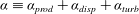
 $$\begin{eqnarray}{\it\alpha}\equiv -\underbrace{\frac{{\it\delta}_{g}}{2{\it\gamma}_{g}}}_{{\it\alpha}_{prod}}+\underbrace{\frac{Q_{m}}{2{\it\gamma}_{g}M_{m}^{5/2}}\frac{\partial }{\partial z}[\left({\it\gamma}_{g}+1-2{\it\beta}_{g}\right)M_{m}^{2}]}_{{\it\alpha}_{disp}}+\underbrace{\frac{Q_{m}}{{\it\gamma}_{g}M_{m}^{3/2}}\left({\it\beta}_{g}-1\right)\frac{\partial M_{m}}{\partial z}}_{{\it\alpha}_{turb}}.\end{eqnarray}$$
Equation (2.22) is different to the volume conservation equation obtained by KTC05 because it describes an unsteady state, without buoyancy, and accounts for a possible dependence of the entrainment coefficient on turbulence transport and pressure. An additional difference is the choice made by KTC05 to define their top-hat radius (cf.
 $r_{m}$
in the present formulation) in terms of profiles of velocity and buoyancy, rather than velocity alone. In both KTC05 and the present formulation the entrainment coefficient is affected by the shape of the longitudinal velocity profile. In an unsteady setting, the use of the mean energy equation has produced the factor
$r_{m}$
in the present formulation) in terms of profiles of velocity and buoyancy, rather than velocity alone. In both KTC05 and the present formulation the entrainment coefficient is affected by the shape of the longitudinal velocity profile. In an unsteady setting, the use of the mean energy equation has produced the factor
 ${\it\gamma}_{g}^{-1}$
in the area equation, whose physical significance as a dimensionless energy flux
${\it\gamma}_{g}^{-1}$
in the area equation, whose physical significance as a dimensionless energy flux
 ${\it\gamma}_{g}$
can now be understood. In the area equation
${\it\gamma}_{g}$
can now be understood. In the area equation
 ${\it\gamma}_{g}$
has the effect of modifying the timescale on which changes in area occur. Alternatively, if
${\it\gamma}_{g}$
has the effect of modifying the timescale on which changes in area occur. Alternatively, if
 ${\it\gamma}_{g}$
remains constant, the first term of (2.22) can be expressed as the temporal derivative of a modified area:
${\it\gamma}_{g}$
remains constant, the first term of (2.22) can be expressed as the temporal derivative of a modified area:
 $\partial _{t}(A_{m}/{\it\gamma}_{g})$
. In either case, these effects are determined by the profile shapes and turbulent transport terms. The derivation of the area equation using the equations for the mean momentum and energy generalises the separate approaches (e.g. top-hat, Gaussian) adopted in unsteady plume models and makes clear their physical implications. Motivation for the particular decomposition used in (2.23) comes from the fact that it separates the influence of the integral intensity of the turbulence and pressure (
$\partial _{t}(A_{m}/{\it\gamma}_{g})$
. In either case, these effects are determined by the profile shapes and turbulent transport terms. The derivation of the area equation using the equations for the mean momentum and energy generalises the separate approaches (e.g. top-hat, Gaussian) adopted in unsteady plume models and makes clear their physical implications. Motivation for the particular decomposition used in (2.23) comes from the fact that it separates the influence of the integral intensity of the turbulence and pressure (
 ${\it\beta}_{g}-1$
) from dispersive effects (
${\it\beta}_{g}-1$
) from dispersive effects (
 ${\it\gamma}_{g}+1-2{\it\beta}_{g}$
).
${\it\gamma}_{g}+1-2{\it\beta}_{g}$
).
The term
 ${\it\alpha}_{prod}$
is the leading-order term responsible for entrainment. It is proportional to the ratio of the dimensionless integral production and redistribution of turbulence kinetic energy
${\it\alpha}_{prod}$
is the leading-order term responsible for entrainment. It is proportional to the ratio of the dimensionless integral production and redistribution of turbulence kinetic energy
 ${\it\delta}_{g}$
, and the gross dimensionless energy flux
${\it\delta}_{g}$
, and the gross dimensionless energy flux
 ${\it\gamma}_{g}$
. Conventionally,
${\it\gamma}_{g}$
. Conventionally,
 ${\it\alpha}_{prod}$
is the only contribution to entrainment that is considered and, in the steady state, gives rise to the classical entrainment coefficient:
${\it\alpha}_{prod}$
is the only contribution to entrainment that is considered and, in the steady state, gives rise to the classical entrainment coefficient:
 $$\begin{eqnarray}{\it\alpha}_{0}\equiv -\frac{{\it\delta}_{g}}{2{\it\gamma}_{g}},\end{eqnarray}$$
where, unless stated otherwise, the value of a quantity
 ${\it\chi}$
in the steady state will be denoted hereafter by
${\it\chi}$
in the steady state will be denoted hereafter by
 ${\it\chi}_{0}$
. In the steady-state equations the independent behaviour of
${\it\chi}_{0}$
. In the steady-state equations the independent behaviour of
 ${\it\delta}_{g}$
and
${\it\delta}_{g}$
and
 ${\it\gamma}_{g}$
is unimportant, as it is only their ratio (2.24) that modifies the governing equations. In an unsteady setting, on the other hand, one finds several additional terms (e.g.
${\it\gamma}_{g}$
is unimportant, as it is only their ratio (2.24) that modifies the governing equations. In an unsteady setting, on the other hand, one finds several additional terms (e.g.
 ${\it\gamma}_{g}^{-1}\partial _{t}A_{m}$
) that depend on
${\it\gamma}_{g}^{-1}\partial _{t}A_{m}$
) that depend on
 ${\it\gamma}_{g}$
independently, which means that the behaviour of both
${\it\gamma}_{g}$
independently, which means that the behaviour of both
 ${\it\gamma}_{g}$
and
${\it\gamma}_{g}$
and
 ${\it\delta}_{g}$
, and not just their ratio, becomes relevant.
${\it\delta}_{g}$
, and not just their ratio, becomes relevant.
Together, the terms
 ${\it\alpha}_{disp}$
and
${\it\alpha}_{disp}$
and
 ${\it\alpha}_{turb}$
account for a difference in the dimensionless flux of momentum compared to the dimensionless flux of energy and, since
${\it\alpha}_{turb}$
account for a difference in the dimensionless flux of momentum compared to the dimensionless flux of energy and, since
 $A_{m}=Q_{m}^{2}/M_{m}$
, the consequent effect that this has on area. Individually
$A_{m}=Q_{m}^{2}/M_{m}$
, the consequent effect that this has on area. Individually
 ${\it\alpha}_{disp}$
and
${\it\alpha}_{disp}$
and
 ${\it\alpha}_{turb}$
are decomposed components of this process, accounting for non-uniform radial profiles and the intensity of turbulent fluxes, respectively. In a steady state, the fact that the dimensionless energy flux is typically greater than the dimensionless momentum flux is inconsequential, because
${\it\alpha}_{turb}$
are decomposed components of this process, accounting for non-uniform radial profiles and the intensity of turbulent fluxes, respectively. In a steady state, the fact that the dimensionless energy flux is typically greater than the dimensionless momentum flux is inconsequential, because
 $\partial _{z}M_{m}=0$
. In an unsteady setting, on the other hand,
$\partial _{z}M_{m}=0$
. In an unsteady setting, on the other hand,
 $\partial _{z}M_{m}\neq 0$
and
$\partial _{z}M_{m}\neq 0$
and
 ${\it\alpha}_{disp}$
and
${\it\alpha}_{disp}$
and
 ${\it\alpha}_{turb}$
play an active role.
${\it\alpha}_{turb}$
play an active role.
The dispersion term
 ${\it\alpha}_{disp}$
can be expanded as
${\it\alpha}_{disp}$
can be expanded as
 $$\begin{eqnarray}{\it\alpha}_{disp}=\underbrace{\frac{Q_{m}}{{\it\gamma}_{g}M_{m}^{3/2}}\left({\it\gamma}_{g}+1-2{\it\beta}_{g}\right)\frac{\partial M_{m}}{\partial z}}_{{\it\alpha}_{disp1}}+\underbrace{\frac{Q_{m}}{2{\it\gamma}_{g}M_{m}^{1/2}}\frac{\partial }{\partial z}\left({\it\gamma}_{g}+1-2{\it\beta}_{g}\right)}_{{\it\alpha}_{disp2}},\end{eqnarray}$$
which makes explicit the individual contributions from dispersion of type I and type II, respectively. When all profiles are self-similar, the gross momentum and energy fluxes can be expressed as a constant proportion of
 $M_{m}$
and
$M_{m}$
and
 $M_{m}^{2}/Q_{m}$
, respectively, therefore the dimensionless fluxes
$M_{m}^{2}/Q_{m}$
, respectively, therefore the dimensionless fluxes
 ${\it\gamma}_{g}$
and
${\it\gamma}_{g}$
and
 ${\it\beta}_{g}$
are constant. In that case, it is evident from (2.25) that
${\it\beta}_{g}$
are constant. In that case, it is evident from (2.25) that
 ${\it\alpha}_{disp2}=0$
. In general however,
${\it\alpha}_{disp2}=0$
. In general however,
 ${\it\alpha}_{disp2}\neq 0$
, which will be the case whenever the longitudinal scaling of the jet variables differs from the asymptotic power-law scaling predicted by similarity theory. If the velocity profiles deform and similarity is lost, the effect of
${\it\alpha}_{disp2}\neq 0$
, which will be the case whenever the longitudinal scaling of the jet variables differs from the asymptotic power-law scaling predicted by similarity theory. If the velocity profiles deform and similarity is lost, the effect of
 ${\it\alpha}_{disp2}$
is to ‘mix’ area in the longitudinal direction. Notably, since
${\it\alpha}_{disp2}$
is to ‘mix’ area in the longitudinal direction. Notably, since
 ${\it\beta}_{g}$
is not an operand of
${\it\beta}_{g}$
is not an operand of
 $\partial _{z}$
in
$\partial _{z}$
in
 ${\it\alpha}_{turb}$
, type II dispersion provides the only source of such mixing. The similarity drift identified by KTC05 also includes the effects of deformation that we label as
${\it\alpha}_{turb}$
, type II dispersion provides the only source of such mixing. The similarity drift identified by KTC05 also includes the effects of deformation that we label as
 ${\it\alpha}_{disp2}$
. However, as the name implies, the similarity drift in KTC05 is used primarily to quantify the effect that a change in the relative widths of the velocity and buoyancy profiles has on entrainment. To refer to
${\it\alpha}_{disp2}$
. However, as the name implies, the similarity drift in KTC05 is used primarily to quantify the effect that a change in the relative widths of the velocity and buoyancy profiles has on entrainment. To refer to
 ${\it\alpha}_{disp2}$
as accounting for similarity drift in the present context is therefore slightly misleading, because here we are concerned with localised deformations in the velocity profile alone, arising from an unsteady forcing. In the present context it is more useful to regard
${\it\alpha}_{disp2}$
as accounting for similarity drift in the present context is therefore slightly misleading, because here we are concerned with localised deformations in the velocity profile alone, arising from an unsteady forcing. In the present context it is more useful to regard
 ${\it\alpha}_{disp2}$
as the effective entrainment, or detrainment, that corresponds to a change in the shape of the velocity profile. For example, in the development of a top-hat velocity profile into a Gaussian velocity profile the flow on the axis of the jet effectively ‘entrains’ from the rest of the jet and hence
${\it\alpha}_{disp2}$
as the effective entrainment, or detrainment, that corresponds to a change in the shape of the velocity profile. For example, in the development of a top-hat velocity profile into a Gaussian velocity profile the flow on the axis of the jet effectively ‘entrains’ from the rest of the jet and hence
 ${\it\alpha}_{disp2}>0$
.
${\it\alpha}_{disp2}>0$
.
The contribution
 ${\it\alpha}_{disp1}$
is perhaps best regarded as a consequence of the spatial acceleration of the flow. Even when the flow evolves in a state of self-similarity,
${\it\alpha}_{disp1}$
is perhaps best regarded as a consequence of the spatial acceleration of the flow. Even when the flow evolves in a state of self-similarity,
 ${\it\alpha}_{disp1}$
will be non-zero in general. Assuming
${\it\alpha}_{disp1}$
will be non-zero in general. Assuming
 ${\it\gamma}_{g}+1-2{\it\beta}_{g}>1$
, positive spatial acceleration (
${\it\gamma}_{g}+1-2{\it\beta}_{g}>1$
, positive spatial acceleration (
 $\partial _{z}M_{m}>0$
) will result in a positive contribution to the entrainment coefficient, whilst negative spatial acceleration (
$\partial _{z}M_{m}>0$
) will result in a positive contribution to the entrainment coefficient, whilst negative spatial acceleration (
 $\partial _{z}M_{m}<0$
) results in a negative contribution to the entrainment coefficient. The role of
$\partial _{z}M_{m}<0$
) results in a negative contribution to the entrainment coefficient. The role of
 ${\it\alpha}_{disp1}$
can therefore be visualised as resulting from a relative convergence or divergence of the flow on a horizontal plane depending on whether
${\it\alpha}_{disp1}$
can therefore be visualised as resulting from a relative convergence or divergence of the flow on a horizontal plane depending on whether
 $\partial _{z}M_{m}$
is greater than or less than zero, respectively. In general, the contribution to entrainment from
$\partial _{z}M_{m}$
is greater than or less than zero, respectively. In general, the contribution to entrainment from
 ${\it\alpha}_{disp1}$
is fundamentally distinct from the Richardson number dependence that emerges in the presence of buoyancy. However, in the special case of statistically steady plumes, in which
${\it\alpha}_{disp1}$
is fundamentally distinct from the Richardson number dependence that emerges in the presence of buoyancy. However, in the special case of statistically steady plumes, in which
 $\partial _{z}M_{m}$
can be replaced with the integral of buoyancy,
$\partial _{z}M_{m}$
can be replaced with the integral of buoyancy,
 ${\it\alpha}_{disp1}$
contributes to the Richardson number dependence identified by PB55 and KTC05.
${\it\alpha}_{disp1}$
contributes to the Richardson number dependence identified by PB55 and KTC05.
2.5. The relation between the classical view of entrainment and turbulence mixing
The classical view of turbulent entrainment in jets pertains to the engulfment of quiescent fluid at the turbulence boundary and is based on the continuity equation. It is therefore useful to consider the relation between the classical view and the energetics perspective advocated in this paper. Below we will argue that the continuity equation demonstrates that fluid is entrained, whilst the mean energy equation provides insight into why the fluid is entrained.
For the purposes of the present discussion we will adopt the classical approach, integrating (2.3) over a disk of radius
 $r_{d}\rightarrow \infty$
and assuming that
$r_{d}\rightarrow \infty$
and assuming that
 $Q_{m}$
remains bounded:
$Q_{m}$
remains bounded:
 $$\begin{eqnarray}\frac{\partial Q_{m}}{\partial z}=-2ru|_{\infty },\end{eqnarray}$$
which simply states that longitudinal changes in the volume flux are accompanied by an induced radial flow in the ambient. Equation (2.26) is an integral continuity equation and is valid for statistically steady and unsteady flows.
In a steady state the mean energy equation is useful (see e.g. Kaminski et al. Reference Kaminski, Tait and Carazzo2005) because it reveals that the strength of the induced flow is equal to the ratio of turbulence production and the energy flux:
 $$\begin{eqnarray}2ru|_{\infty }=\frac{{\it\delta}_{g}}{{\it\gamma}_{g}}w_{m}r_{m}.\end{eqnarray}$$
Hence, the mean energy equation provides insight into why fluid is being entrained into the jet. If turbulence production were equal to zero there would be no induced flow in the ambient and
 $\partial _{z}Q_{m}=0$
. In a steady state the induced flow
$\partial _{z}Q_{m}=0$
. In a steady state the induced flow
 $ru|_{\infty }$
is equal to the rate at which fluid is entrained into the jet. However, in a statistically unsteady situation (2.26) is of limited use because it does not necessarily describe the rate at which ambient fluid is entrained into the jet. Indeed, the radius of the jet
$ru|_{\infty }$
is equal to the rate at which fluid is entrained into the jet. However, in a statistically unsteady situation (2.26) is of limited use because it does not necessarily describe the rate at which ambient fluid is entrained into the jet. Indeed, the radius of the jet
 $r_{m}\equiv Q_{m}/M_{m}^{(1/2)}$
might vary with time, which would mean that the rate at which fluid enters the jet does not correspond to the induced flow in the ambient.
$r_{m}\equiv Q_{m}/M_{m}^{(1/2)}$
might vary with time, which would mean that the rate at which fluid enters the jet does not correspond to the induced flow in the ambient.
In a statistically unsteady situation the mean energy equation is useful because, since it pertains to why fluid is entrained, it is able to go further than (2.26) and predict the rate at which fluid is entrained into the jet. Using (2.26) and the area equation (2.22), which was obtained from integral equations for the mean momentum (2.12) and energy (2.13),
 $$\begin{eqnarray}2ru|_{\infty }-\frac{2r_{m}}{{\it\gamma}_{g}}\frac{\partial r_{m}}{\partial t}=-2{\it\alpha}r_{m}w_{m},\end{eqnarray}$$
where the entrainment coefficient
 ${\it\alpha}\equiv {\it\alpha}_{prod}+{\it\alpha}_{disp}+{\it\alpha}_{turb}$
has a known dependence on the physical properties of the jet. Equation (2.28) states that
${\it\alpha}\equiv {\it\alpha}_{prod}+{\it\alpha}_{disp}+{\it\alpha}_{turb}$
has a known dependence on the physical properties of the jet. Equation (2.28) states that
 $-2{\it\alpha}r_{m}w_{m}$
is the rate of entrainment relative to the inward/outward propagation rate of a characteristic jet radius at a fixed longitudinal location (for a discussion of several alternative definitions of an entrainment velocity the reader is referred to Turner Reference Turner1986). However, in jets that do not have a top-hat profile the edge of the jet is not always clearly defined. Evident from the left-hand side of (2.28) is that the appropriate radius from which to view entrainment is the effective entrainment radius
$-2{\it\alpha}r_{m}w_{m}$
is the rate of entrainment relative to the inward/outward propagation rate of a characteristic jet radius at a fixed longitudinal location (for a discussion of several alternative definitions of an entrainment velocity the reader is referred to Turner Reference Turner1986). However, in jets that do not have a top-hat profile the edge of the jet is not always clearly defined. Evident from the left-hand side of (2.28) is that the appropriate radius from which to view entrainment is the effective entrainment radius
 $r_{m}{\it\gamma}_{g}^{-1/2}$
, which is determined by the radial dependence of the jet’s longitudinal velocity profile. As one would expect, for a top-hat jet with
$r_{m}{\it\gamma}_{g}^{-1/2}$
, which is determined by the radial dependence of the jet’s longitudinal velocity profile. As one would expect, for a top-hat jet with
 ${\it\gamma}_{g}=1$
, the effective entrainment radius coincides with the radius
${\it\gamma}_{g}=1$
, the effective entrainment radius coincides with the radius
 $r_{m}$
. For a temporal jet
$r_{m}$
. For a temporal jet
 $\partial _{z}Q_{m}=0$
and therefore, using (2.26),
$\partial _{z}Q_{m}=0$
and therefore, using (2.26),
 $ru|_{\infty }=0$
. In that case, (2.28) indicates that the entrainment flux
$ru|_{\infty }=0$
. In that case, (2.28) indicates that the entrainment flux
 $-2{\it\alpha}r_{m}w_{m}$
is equal in magnitude and opposite in sign to the time rate of change of the effective area
$-2{\it\alpha}r_{m}w_{m}$
is equal in magnitude and opposite in sign to the time rate of change of the effective area
 $r_{m}^{2}{\it\gamma}_{g}^{-1}$
.
$r_{m}^{2}{\it\gamma}_{g}^{-1}$
.
Note that even though the momentum–energy framework naturally includes turbulence, it remains an integral-scale description that is not concerned with the small-scale aspects of turbulence. Consequently, we do not make statements about the dynamics of the turbulent–non-turbulent interface (see e.g. da Silva et al. Reference da Silva, Hunt, Eames and Westerweel2014, for details), although large-scale and small-scale entrainment are intimately connected (see van Reeuwijk & Holzner Reference van Reeuwijk and Holzner2014).
3. Simulation details
The data presented herein were obtained from direct simulation of the full Navier–Stokes equations. For spatial discretisation we use a formulation that is equivalent to the fourth-order-accurate discretisation described by Verstappen & Veldman (Reference Verstappen and Veldman2003). The scheme employs central differences throughout and is conservative in mass, momentum and energy. Time integration is performed using a third-order Adams–Bashforth scheme with an adaptive step size that is determined by a local stability criterion. As the code was recently upgraded from second to fourth order, a brief description of the code and verification results are provided in appendix A.
In all simulations we use a domain of size approximately
 $44^{2}\times 66$
source radii,
$44^{2}\times 66$
source radii,
 $r_{0}$
, in the horizontal and longitudinal directions, respectively. The base of the domain consists of a free-slip surface surrounding a centralised source of constant momentum flux
$r_{0}$
, in the horizontal and longitudinal directions, respectively. The base of the domain consists of a free-slip surface surrounding a centralised source of constant momentum flux
 $M_{0}$
and constant volume flux
$M_{0}$
and constant volume flux
 $Q_{0}$
, which provide the definition for the source radius as
$Q_{0}$
, which provide the definition for the source radius as
 $$\begin{eqnarray}r_{0}\equiv \frac{Q_{0}}{M_{0}^{1/2}},\end{eqnarray}$$
and the Reynolds number,
 $\mathit{Re}_{0}\equiv 2M_{0}^{1/2}/{\it\nu}$
.
$\mathit{Re}_{0}\equiv 2M_{0}^{1/2}/{\it\nu}$
.
We simulate two steady-state cases, L and H, of Reynolds numbers 4815 and 6810, respectively. Data for these cases are collected over approximately
 $t_{run}/{\it\tau}_{0}=3000$
dimensionless time units, where the source turnover time
$t_{run}/{\it\tau}_{0}=3000$
dimensionless time units, where the source turnover time
 ${\it\tau}_{0}=Q_{0}^{2}/M_{0}^{3/2}$
. We eliminate initial transients from the problem by running the simulations for not less than 3000 dimensionless time units before collecting statistics. Although the sampling time and our allowance for transient behaviour appears to be excessively large, it should be noted that the turnover time in a jet scales in the longitudinal direction according to
${\it\tau}_{0}=Q_{0}^{2}/M_{0}^{3/2}$
. We eliminate initial transients from the problem by running the simulations for not less than 3000 dimensionless time units before collecting statistics. Although the sampling time and our allowance for transient behaviour appears to be excessively large, it should be noted that the turnover time in a jet scales in the longitudinal direction according to
 $z^{2}$
.
$z^{2}$
.
The domain is discretised using a uniform computational grid of
 $768^{2}\times 1152$
cells, with source resolution of 48 cells over the physical source diameter, which corresponds to approximately 34 cells over
$768^{2}\times 1152$
cells, with source resolution of 48 cells over the physical source diameter, which corresponds to approximately 34 cells over
 $2r_{0}$
. The difference between the physical source diameter and
$2r_{0}$
. The difference between the physical source diameter and
 $2r_{0}$
is due to the use of a gauze, which will be described below. Simulation
$2r_{0}$
is due to the use of a gauze, which will be described below. Simulation
 $\text{H}^{\ast }$
, which is used to check the convergence of the results, employs a grid of
$\text{H}^{\ast }$
, which is used to check the convergence of the results, employs a grid of
 $512^{2}\times 768$
cells. Open boundary conditions are used to allow fluid to enter and leave the computational domain. In particular, the inflow boundary condition on the vertical faces of the domain accounts for the flow’s axisymmetry and the outflow boundary condition on the top face of the domain consists of a convective boundary condition that adjusts dynamically to a non-uniformly distributed wall-normal velocity. Further details and testing of the boundary conditions we employ can be found in Craske & van Reeuwijk (Reference Craske and van Reeuwijk2013). To initiate the turbulence we apply perturbations of 1 % to the velocities in the first cell above the source. A disadvantage with simply connected circular sources of momentum flux is that they result in a potential core region, of approximately
$512^{2}\times 768$
cells. Open boundary conditions are used to allow fluid to enter and leave the computational domain. In particular, the inflow boundary condition on the vertical faces of the domain accounts for the flow’s axisymmetry and the outflow boundary condition on the top face of the domain consists of a convective boundary condition that adjusts dynamically to a non-uniformly distributed wall-normal velocity. Further details and testing of the boundary conditions we employ can be found in Craske & van Reeuwijk (Reference Craske and van Reeuwijk2013). To initiate the turbulence we apply perturbations of 1 % to the velocities in the first cell above the source. A disadvantage with simply connected circular sources of momentum flux is that they result in a potential core region, of approximately
 $10r_{0}$
in longitudinal extent (Rajaratnam Reference Rajaratnam1976), preceding the region of fully developed flow, in which we are primarily interested. To reduce the longitudinal extent of the potential core we employ the numerical equivalent of a gauze used in experiments (see e.g. Hunt & Linden Reference Hunt and Linden2001), by obstructing a purely circular source with two centralised orthogonal strips, thereby disconnecting the source into four identical discrete segments. Consequently, the effective source radius defined in (3.1) is slightly smaller than the physical extent of the source, whose overall diameter is spanned by 48 cells. It should be noted that simulations without the gauze yield similar results in the far field to those presented here, albeit with a smaller far-field region.
$10r_{0}$
in longitudinal extent (Rajaratnam Reference Rajaratnam1976), preceding the region of fully developed flow, in which we are primarily interested. To reduce the longitudinal extent of the potential core we employ the numerical equivalent of a gauze used in experiments (see e.g. Hunt & Linden Reference Hunt and Linden2001), by obstructing a purely circular source with two centralised orthogonal strips, thereby disconnecting the source into four identical discrete segments. Consequently, the effective source radius defined in (3.1) is slightly smaller than the physical extent of the source, whose overall diameter is spanned by 48 cells. It should be noted that simulations without the gauze yield similar results in the far field to those presented here, albeit with a smaller far-field region.
For the unsteady simulations we impose a step change in the source momentum flux, doubling and halving
 $M_{0}$
for the cases LH and HL, respectively, while keeping the source radius constant. To ensure reliable statistics we carry out an ensemble of simulations. Initial conditions for LH and HL were obtained from the two steady-state base simulations, L and H, respectively. During the course of one of these base simulations we write 16 complete three-dimensional field files to disk at dimensionless time intervals not less than 200 units. The field files from each of the two base cases provide the initial conditions for an ensemble of 16 independent statistically unsteady simulations. In the case of the steady simulations we obtain statistics by averaging over time and the homogeneous azimuthal dimension. In the case of the unsteady simulations however, the time dimension is no longer statistically homogeneous. We therefore reduce the time interval over which averages are taken to not more than
$M_{0}$
for the cases LH and HL, respectively, while keeping the source radius constant. To ensure reliable statistics we carry out an ensemble of simulations. Initial conditions for LH and HL were obtained from the two steady-state base simulations, L and H, respectively. During the course of one of these base simulations we write 16 complete three-dimensional field files to disk at dimensionless time intervals not less than 200 units. The field files from each of the two base cases provide the initial conditions for an ensemble of 16 independent statistically unsteady simulations. In the case of the steady simulations we obtain statistics by averaging over time and the homogeneous azimuthal dimension. In the case of the unsteady simulations however, the time dimension is no longer statistically homogeneous. We therefore reduce the time interval over which averages are taken to not more than
 $2{\it\tau}_{0}$
, and average over the ensemble, in addition to the azimuthal direction. From the unsteady simulations, which are each of approximate duration
$2{\it\tau}_{0}$
, and average over the ensemble, in addition to the azimuthal direction. From the unsteady simulations, which are each of approximate duration
 $200{\it\tau}_{0}$
, we obtain a sequence of 120 files describing the ensemble-averaged behaviour of the variables over the inhomogeneous spatial dimensions
$200{\it\tau}_{0}$
, we obtain a sequence of 120 files describing the ensemble-averaged behaviour of the variables over the inhomogeneous spatial dimensions
 $r$
and
$r$
and
 $z$
. Details of the simulations performed can be found in table 1.
$z$
. Details of the simulations performed can be found in table 1.
Simulation details. Here
 $M_{0}^{B}$
and
$M_{0}^{B}$
and
 $M_{0}^{A}$
are the source momentum fluxes before and after the step change, respectively.
$M_{0}^{A}$
are the source momentum fluxes before and after the step change, respectively.

Dimensionless profiles of longitudinal velocity (a), longitudinal velocity variance (b) and Reynolds stress (c). The simulation data are compared to the experimental data of Panchapakesan & Lumley (Reference Panchapakesan and Lumley1993, PL93) and Ezzamel, Salizzoni & Hunt (Reference Ezzamel Ezzamel, Salizzoni and Hunt2015, ESH15). The displayed simulation data consist of approximately 80 different radial profiles taken from the interval
 $z/r_{0}\in [28,55]$
. The experimental data from ESH15 and PL93 were obtained from the single location
$z/r_{0}\in [28,55]$
. The experimental data from ESH15 and PL93 were obtained from the single location
 $z/r_{0}=30$
and an average over the interval
$z/r_{0}=30$
and an average over the interval
 $z/r_{0}\in [120,240]$
, respectively.
$z/r_{0}\in [120,240]$
, respectively.

Azimuthally averaged data over cylindrical coordinates are obtained by partitioning the domain into cylindrical shells. The location of the centre of each small square control volume in the domain determines the shell to which it belongs, and the total number of control volumes belonging to a given shell determines the area allocated to the shell. In this way integrals over
 $r$
are equivalent to integrals over all volumes lying within a given disk. To determine the upper limit of integrals over the radial dimension, we use
$r$
are equivalent to integrals over all volumes lying within a given disk. To determine the upper limit of integrals over the radial dimension, we use
 ${\it\epsilon}\equiv 0.01$
in (2.9). It is not possible to follow the classical definitions of
${\it\epsilon}\equiv 0.01$
in (2.9). It is not possible to follow the classical definitions of
 $Q_{m}$
and
$Q_{m}$
and
 $M_{m}$
by integrating over the interval
$M_{m}$
by integrating over the interval
 $[0,\infty ]$
on any domain of finite extent.
$[0,\infty ]$
on any domain of finite extent.
4. Results
4.1. Validation
In figure 2 we compare radial profiles of mean longitudinal velocity
 $\overline{w}$
, longitudinal velocity variance
$\overline{w}$
, longitudinal velocity variance
 $\overline{w^{\prime 2}}$
, and the Reynolds stress
$\overline{w^{\prime 2}}$
, and the Reynolds stress
 $\overline{u^{\prime }w^{\prime }}$
, to the experimental data of Panchapakesan & Lumley (Reference Panchapakesan and Lumley1993) and Ezzamel et al. (Reference Ezzamel Ezzamel, Salizzoni and Hunt2015), hereafter referred to as PL93 and ESH15, respectively. Figure 2 displays approximately 80 radial profiles from the simulation data, each taken from the interval
$\overline{u^{\prime }w^{\prime }}$
, to the experimental data of Panchapakesan & Lumley (Reference Panchapakesan and Lumley1993) and Ezzamel et al. (Reference Ezzamel Ezzamel, Salizzoni and Hunt2015), hereafter referred to as PL93 and ESH15, respectively. Figure 2 displays approximately 80 radial profiles from the simulation data, each taken from the interval
 $z/r_{0}\in [28,55]$
and normalised using
$z/r_{0}\in [28,55]$
and normalised using
 $r_{m}(z)$
and
$r_{m}(z)$
and
 $w_{m}(z)$
. The same normalisation was applied to the experimental data, although in PL93 the interval from which the data were obtained was
$w_{m}(z)$
. The same normalisation was applied to the experimental data, although in PL93 the interval from which the data were obtained was
 $z/r_{0}\in [120,240]$
and in ESH15 the data correspond to the single location
$z/r_{0}\in [120,240]$
and in ESH15 the data correspond to the single location
 $z/r_{0}=30$
. In the mean longitudinal velocity shown in figure 2(a) the simulation results exhibit a good collapse relative to each other, and to both ESH15 and PL93. In figure 2(b) it is evident that the simulation results approximately reproduce both the amplitude and the radial dependence of the dimensionless turbulent transport
$z/r_{0}=30$
. In the mean longitudinal velocity shown in figure 2(a) the simulation results exhibit a good collapse relative to each other, and to both ESH15 and PL93. In figure 2(b) it is evident that the simulation results approximately reproduce both the amplitude and the radial dependence of the dimensionless turbulent transport
 $\overline{w^{\prime 2}}/w_{m}^{2}$
found in ESH15. With respect to PL93, the turbulent transport
$\overline{w^{\prime 2}}/w_{m}^{2}$
found in ESH15. With respect to PL93, the turbulent transport
 $\overline{w^{\prime 2}}/w_{m}^{2}$
in both the simulation data and ESH15 is smaller in amplitude, although it has a similar radial dependence. The likely cause of this difference is the fact that the normalised longitudinal fluctuations
$\overline{w^{\prime 2}}/w_{m}^{2}$
in both the simulation data and ESH15 is smaller in amplitude, although it has a similar radial dependence. The likely cause of this difference is the fact that the normalised longitudinal fluctuations
 $w^{\prime }/w_{m}$
adjust to equilibrium over extremely large distances. Indeed, PL93 point out that equilibrium is not attained until approximately
$w^{\prime }/w_{m}$
adjust to equilibrium over extremely large distances. Indeed, PL93 point out that equilibrium is not attained until approximately
 $z/r_{0}=140$
. However, the effect that this has on the integral quantities in the jet is smaller than one might expect, because the values most strongly affected are concentrated on the centreline. In the Reynolds stress
$z/r_{0}=140$
. However, the effect that this has on the integral quantities in the jet is smaller than one might expect, because the values most strongly affected are concentrated on the centreline. In the Reynolds stress
 $\overline{u^{\prime }w^{\prime }}$
shown in figure 2(c) the numerical results exhibit a good agreement with those of ESH15, whose amplitude again lies slightly beneath the far-field data of PL93.
$\overline{u^{\prime }w^{\prime }}$
shown in figure 2(c) the numerical results exhibit a good agreement with those of ESH15, whose amplitude again lies slightly beneath the far-field data of PL93.
(a) Isoregions of instantaneous longitudinal velocity
 $w(r,{\rm\pi},z,t_{0})$
, where
$w(r,{\rm\pi},z,t_{0})$
, where
 $t_{0}\approx 1200{\it\tau}_{0}$
(left-hand side), and average longitudinal velocity
$t_{0}\approx 1200{\it\tau}_{0}$
(left-hand side), and average longitudinal velocity
 $\overline{w}(r,z)$
(right-hand side), with darker shades corresponding to larger values. A linear fit to the theoretical plume width
$\overline{w}(r,z)$
(right-hand side), with darker shades corresponding to larger values. A linear fit to the theoretical plume width
 $r_{m}=2{\it\alpha}_{0}(z-z_{v})$
is indicated on the right hand side with a solid grey line, in addition to streamlines of the induced ambient flow. (b) Normalised volume flux
$r_{m}=2{\it\alpha}_{0}(z-z_{v})$
is indicated on the right hand side with a solid grey line, in addition to streamlines of the induced ambient flow. (b) Normalised volume flux
 $Q_{m}/(r_{0}M_{m0}^{1/2})$
and (c) momentum flux
$Q_{m}/(r_{0}M_{m0}^{1/2})$
and (c) momentum flux
 $M_{m}/M_{m0}$
. The interval
$M_{m}/M_{m0}$
. The interval
 $[z_{b},z_{t}]$
, used in (4.1) to obtain the steady-state momentum flux
$[z_{b},z_{t}]$
, used in (4.1) to obtain the steady-state momentum flux
 $M_{m0}$
, is indicated on the left-hand side of (a).
$M_{m0}$
, is indicated on the left-hand side of (a).

Using time traces of the centreline velocity
 $w(0,z,t)$
at
$w(0,z,t)$
at
 $z/r_{0}=44$
and the Taylor hypothesis, one-dimensional spectra were obtained. An estimation of the dissipation rate was calculated according to
$z/r_{0}=44$
and the Taylor hypothesis, one-dimensional spectra were obtained. An estimation of the dissipation rate was calculated according to
 ${\it\varepsilon}\approx 15{\it\nu}\overline{(\partial _{t}w^{\prime })^{2}}/\overline{w}^{2}$
. The peak of the dissipation spectrum at
${\it\varepsilon}\approx 15{\it\nu}\overline{(\partial _{t}w^{\prime })^{2}}/\overline{w}^{2}$
. The peak of the dissipation spectrum at
 $z/r_{0}=44$
was observed to occur at a length scale corresponding to four times the spacing of the grid. The Taylor Reynolds number for the flow, defined according to
$z/r_{0}=44$
was observed to occur at a length scale corresponding to four times the spacing of the grid. The Taylor Reynolds number for the flow, defined according to
 $\mathit{Re}_{{\it\lambda}}\equiv \overline{w^{\prime 2}}\sqrt{15/{\it\varepsilon}{\it\nu}}$
(Tennekes & Lumley Reference Tennekes and Lumley1972), was found to be equal to 100 and 135 in simulations L and H, respectively.
$\mathit{Re}_{{\it\lambda}}\equiv \overline{w^{\prime 2}}\sqrt{15/{\it\varepsilon}{\it\nu}}$
(Tennekes & Lumley Reference Tennekes and Lumley1972), was found to be equal to 100 and 135 in simulations L and H, respectively.
4.2. The steady jet
Figure 3(a) shows an instantaneous and time-averaged slice through the longitudinal velocity field. Notable is the fact that entrainment into the jet is established close to the source, which is evident in the positive, and almost uniform, gradient of
 $Q_{m}$
for
$Q_{m}$
for
 $z/r_{0}>0$
. In figure 3(b,c) we display the longitudinal variation of
$z/r_{0}>0$
. In figure 3(b,c) we display the longitudinal variation of
 $Q_{m}$
and
$Q_{m}$
and
 $M_{m}$
in simulations L, H and
$M_{m}$
in simulations L, H and
 $\text{H}^{\ast }$
. Since plume theory only pertains to mean quantities, it is necessary to define a steady-state momentum flux:
$\text{H}^{\ast }$
. Since plume theory only pertains to mean quantities, it is necessary to define a steady-state momentum flux:
 $$\begin{eqnarray}M_{m0}\equiv \frac{1}{z_{t}-z_{b}}\int _{z_{b}}^{z_{t}}M_{m}\text{d}z\leqslant M_{0},\end{eqnarray}$$
where
 $z_{b}/r_{0}=28$
and
$z_{b}/r_{0}=28$
and
 $z_{t}/r_{0}=55$
, which, as expected, results in a good collapse of the simulation data from L, H and
$z_{t}/r_{0}=55$
, which, as expected, results in a good collapse of the simulation data from L, H and
 $\text{H}^{\ast }$
. From dimensional analysis it follows that
$\text{H}^{\ast }$
. From dimensional analysis it follows that
 $M_{m}$
should be constant and
$M_{m}$
should be constant and
 $Q_{m}$
proportional to
$Q_{m}$
proportional to
 $z/r_{0}$
, which is confirmed in the simulation results. At the top of the domain the linear behaviour in
$z/r_{0}$
, which is confirmed in the simulation results. At the top of the domain the linear behaviour in
 $Q_{m}$
is slightly affected by an inclination of the streamlines in the ambient, which influences the integration limit
$Q_{m}$
is slightly affected by an inclination of the streamlines in the ambient, which influences the integration limit
 $r_{d}$
. A steady-state entrainment coefficient
$r_{d}$
. A steady-state entrainment coefficient
 ${\it\alpha}_{0}$
and virtual origin
${\it\alpha}_{0}$
and virtual origin
 $z_{v}$
were determined for each jet by fitting a straight line to
$z_{v}$
were determined for each jet by fitting a straight line to
 $Q_{m}(z)$
over the interval
$Q_{m}(z)$
over the interval
 $z\in [z_{b},z_{t}]$
, to give
$z\in [z_{b},z_{t}]$
, to give
 ${\it\alpha}_{0}=0.067$
and
${\it\alpha}_{0}=0.067$
and
 $z_{v}/r_{0}=-5.0$
, when averaged over simulations L and H. Hereafter we will use the notation
$z_{v}/r_{0}=-5.0$
, when averaged over simulations L and H. Hereafter we will use the notation
 $Q_{m0}=2{\it\alpha}_{0}M_{m0}^{1/2}(z-z_{v})$
to denote the theoretical steady volume flux in the jet.
$Q_{m0}=2{\it\alpha}_{0}M_{m0}^{1/2}(z-z_{v})$
to denote the theoretical steady volume flux in the jet.
Dimensionless momentum flux
 ${\it\beta}_{g}$
(a,d), dimensionless energy flux
${\it\beta}_{g}$
(a,d), dimensionless energy flux
 ${\it\gamma}_{g}$
(b,e), dimensionless turbulence production and pressure redistribution
${\it\gamma}_{g}$
(b,e), dimensionless turbulence production and pressure redistribution
 ${\it\delta}_{g}$
(c, f), and their constituent parts, in a steady jet. (a–c) The leading-order components; (d–f) higher-order components. Thin lines correspond to results from L, and thick lines correspond to results from H. Constant values corresponding to a Gaussian profile are displayed as vertical lines in (b,c). The interval over which averaging was performed to obtain the values reported in table 2 is indicated on the left-hand side of (a).
${\it\delta}_{g}$
(c, f), and their constituent parts, in a steady jet. (a–c) The leading-order components; (d–f) higher-order components. Thin lines correspond to results from L, and thick lines correspond to results from H. Constant values corresponding to a Gaussian profile are displayed as vertical lines in (b,c). The interval over which averaging was performed to obtain the values reported in table 2 is indicated on the left-hand side of (a).

The entrainment coefficient
 ${\it\alpha}(z)$
and its constituent parts. Data for H and L shown in dark grey, large symbols (blue online) and light grey, small symbols (red online), respectively. The interval
${\it\alpha}(z)$
and its constituent parts. Data for H and L shown in dark grey, large symbols (blue online) and light grey, small symbols (red online), respectively. The interval
 $z/r_{0}\in [28,55]$
, over which averaging was performed to obtain the value
$z/r_{0}\in [28,55]$
, over which averaging was performed to obtain the value
 ${\it\alpha}_{0}=0.067$
, is indicated on the right-hand side of the figure.
${\it\alpha}_{0}=0.067$
, is indicated on the right-hand side of the figure.

Figure 4 displays longitudinal profiles of
 ${\it\beta}_{g}$
,
${\it\beta}_{g}$
,
 ${\it\gamma}_{g}$
and
${\it\gamma}_{g}$
and
 ${\it\delta}_{g}$
, and their constituent parts, which represent the dimensionless momentum flux, energy flux and turbulence production, respectively. The almost identical behaviour of these variables in L and H confirms that the statistics examined are practically independent of Reynolds number. Here, we are focusing on the dimensionless quantities, e.g.
${\it\delta}_{g}$
, and their constituent parts, which represent the dimensionless momentum flux, energy flux and turbulence production, respectively. The almost identical behaviour of these variables in L and H confirms that the statistics examined are practically independent of Reynolds number. Here, we are focusing on the dimensionless quantities, e.g.
 $M_{f}/M_{m}$
, whose value should be independent of the dependent variables
$M_{f}/M_{m}$
, whose value should be independent of the dependent variables
 $Q_{m}$
and
$Q_{m}$
and
 $M_{m}$
. The dimensionless quantities therefore indicate the relative contribution that is made by all integrals appearing in the governing integral equations (2.11)–(2.13). Of significance is the fact that the values of the dimensionless quantities differ, in some cases considerably, from those that are frequently assumed in models of steady and unsteady jets (see e.g. Morton et al.
Reference Morton, Taylor and Turner1956; Scase et al.
Reference Scase, Caulfield, Dalziel and Hunt2006). As can be judged from the profile of
$M_{m}$
. The dimensionless quantities therefore indicate the relative contribution that is made by all integrals appearing in the governing integral equations (2.11)–(2.13). Of significance is the fact that the values of the dimensionless quantities differ, in some cases considerably, from those that are frequently assumed in models of steady and unsteady jets (see e.g. Morton et al.
Reference Morton, Taylor and Turner1956; Scase et al.
Reference Scase, Caulfield, Dalziel and Hunt2006). As can be judged from the profile of
 ${\it\beta}_{f}\equiv M_{f}/M_{m}$
in figure 4(d), despite the central role that turbulence plays in mixing momentum locally, turbulent transport terms at the integral level are an order of magnitude smaller than those associated with the mean flow, but not insignificant. This observation is consistent with previous findings from experiments, including PL93 and Hussein, Capp & George (Reference Hussein, Capp and George1994). In fact, in
${\it\beta}_{f}\equiv M_{f}/M_{m}$
in figure 4(d), despite the central role that turbulence plays in mixing momentum locally, turbulent transport terms at the integral level are an order of magnitude smaller than those associated with the mean flow, but not insignificant. This observation is consistent with previous findings from experiments, including PL93 and Hussein, Capp & George (Reference Hussein, Capp and George1994). In fact, in
 ${\it\beta}_{p}$
it is seen that a large portion of the turbulent transport of momentum flux is balanced by a reduction of pressure in the jet, which can be estimated to a good approximation using the transverse components of momentum flux
${\it\beta}_{p}$
it is seen that a large portion of the turbulent transport of momentum flux is balanced by a reduction of pressure in the jet, which can be estimated to a good approximation using the transverse components of momentum flux
 $M_{u}$
and
$M_{u}$
and
 $M_{v}$
(see e.g. Hussein et al.
Reference Hussein, Capp and George1994):
$M_{v}$
(see e.g. Hussein et al.
Reference Hussein, Capp and George1994):
 $$\begin{eqnarray}{\it\beta}_{p}=-{\textstyle \frac{1}{2}}({\it\beta}_{u}+{\it\beta}_{v}),\end{eqnarray}$$
where
 $$\begin{eqnarray}{\it\beta}_{u}\equiv \frac{2}{M_{m}}\int _{0}^{r_{d}(z,t)}\overline{u^{\prime 2}}r\text{d}r,\quad {\it\beta}_{v}\equiv \frac{2}{M_{m}}\int _{0}^{r_{d}(z,t)}\overline{v^{\prime 2}}r\text{d}r.\end{eqnarray}$$
In sum, the contribution to the gross momentum flux from pressure and turbulence accounts for approximately 7 %.
Figure 4(b,e) displays dimensionless energy fluxes and confirms that
 ${\it\gamma}_{m}>1$
, which is consistent with the non-uniform profiles that one expects to find in real jets. At
${\it\gamma}_{m}>1$
, which is consistent with the non-uniform profiles that one expects to find in real jets. At
 $z/r_{0}\approx 20$
the dimensionless energy flux
$z/r_{0}\approx 20$
the dimensionless energy flux
 ${\it\gamma}_{m}$
appears to have converged to approximately 1.3, which is close to the exact value of
${\it\gamma}_{m}$
appears to have converged to approximately 1.3, which is close to the exact value of
 ${\it\gamma}_{m}=4/3$
that one would expect to see if the mean flow were perfectly Gaussian, and indicates the presence of dispersion. Below
${\it\gamma}_{m}=4/3$
that one would expect to see if the mean flow were perfectly Gaussian, and indicates the presence of dispersion. Below
 $z/r_{0}=15$
, the jet develops from patches of uniform velocity into a developed flow with significant radial dependence, resulting in the monotonic increase of
$z/r_{0}=15$
, the jet develops from patches of uniform velocity into a developed flow with significant radial dependence, resulting in the monotonic increase of
 ${\it\gamma}_{m}$
from 1 to 1.3. The gross energy flux
${\it\gamma}_{m}$
from 1 to 1.3. The gross energy flux
 ${\it\gamma}_{g}$
is slightly higher than the mean energy flux because the turbulent transport of mean energy
${\it\gamma}_{g}$
is slightly higher than the mean energy flux because the turbulent transport of mean energy
 ${\it\gamma}_{f}$
exceeds the negative pressure-work term
${\it\gamma}_{f}$
exceeds the negative pressure-work term
 ${\it\gamma}_{p}$
, as seen in figure 4(e). Very close to the source, where
${\it\gamma}_{p}$
, as seen in figure 4(e). Very close to the source, where
 $z/r_{0}<5$
, the azimuthal inhomogeneity resulting from the source condition (see § 3) is evidenced in large values of the variance
$z/r_{0}<5$
, the azimuthal inhomogeneity resulting from the source condition (see § 3) is evidenced in large values of the variance
 $\overline{w^{\prime 2}}$
and therefore in large values of
$\overline{w^{\prime 2}}$
and therefore in large values of
 ${\it\beta}_{f}$
and
${\it\beta}_{f}$
and
 ${\it\gamma}_{f}$
. Further from the source, beyond the visible local minimum in
${\it\gamma}_{f}$
. Further from the source, beyond the visible local minimum in
 ${\it\beta}_{f}$
and
${\it\beta}_{f}$
and
 ${\it\gamma}_{f}$
, the flow becomes azimuthally homogeneous and
${\it\gamma}_{f}$
, the flow becomes azimuthally homogeneous and
 ${\it\beta}_{f}$
and
${\it\beta}_{f}$
and
 ${\it\gamma}_{f}$
are approximately constant.
${\it\gamma}_{f}$
are approximately constant.
In the dimensionless production term
 ${\it\delta}_{m}$
in figure 4(c), one sees that an approximately constant value is not established until
${\it\delta}_{m}$
in figure 4(c), one sees that an approximately constant value is not established until
 $z/r_{0}>20$
. Below this height, although one might expect to see a reduction in the entrainment into the jet, since
$z/r_{0}>20$
. Below this height, although one might expect to see a reduction in the entrainment into the jet, since
 ${\it\alpha}_{0}\sim -{\it\delta}_{m}/2{\it\gamma}_{m}$
, the steady increase in
${\it\alpha}_{0}\sim -{\it\delta}_{m}/2{\it\gamma}_{m}$
, the steady increase in
 $-{\it\delta}_{m}$
is approximately balanced by the steady increase in
$-{\it\delta}_{m}$
is approximately balanced by the steady increase in
 ${\it\gamma}_{m}$
. This is an example of the way in which the independent behaviour of
${\it\gamma}_{m}$
. This is an example of the way in which the independent behaviour of
 ${\it\gamma}_{m}$
and
${\it\gamma}_{m}$
and
 ${\it\delta}_{m}$
is unimportant in the steady jet equations.
${\it\delta}_{m}$
is unimportant in the steady jet equations.
Figure 5 displays the constituent parts of the entrainment coefficient (2.23), for both L and H. A moving-average filter of dimensionless length one was applied to raw data in order to obtain the data displayed in figure 5. The close agreement between
 ${\it\alpha}$
and
${\it\alpha}$
and
 $(\partial _{z}Q_{m})/2M_{m}^{1/2}$
implies that the integral equations for momentum (2.12) and energy (2.13), and therefore area (2.11), are satisfied by the simulation data. As expected, the term
$(\partial _{z}Q_{m})/2M_{m}^{1/2}$
implies that the integral equations for momentum (2.12) and energy (2.13), and therefore area (2.11), are satisfied by the simulation data. As expected, the term
 ${\it\alpha}_{prod}$
dominates in the steady state, and provides an excellent means of inferring an entrainment coefficient in a way that is independent, yet consistent, with the direct calculation of
${\it\alpha}_{prod}$
dominates in the steady state, and provides an excellent means of inferring an entrainment coefficient in a way that is independent, yet consistent, with the direct calculation of
 $(\partial _{z}Q_{m})/2M_{m}^{1/2}$
. However, close to the source the role of
$(\partial _{z}Q_{m})/2M_{m}^{1/2}$
. However, close to the source the role of
 ${\it\alpha}_{disp2}$
, whose effects are contained in the similarity drift term in KTC05, is also discernible. There,
${\it\alpha}_{disp2}$
, whose effects are contained in the similarity drift term in KTC05, is also discernible. There,
 ${\it\alpha}_{disp2}$
has the effect of making a positive contribution to entrainment, which is the result of a gradual deformation of the source velocity profile over the region of flow development. Correspondingly, in this region
${\it\alpha}_{disp2}$
has the effect of making a positive contribution to entrainment, which is the result of a gradual deformation of the source velocity profile over the region of flow development. Correspondingly, in this region
 ${\it\alpha}_{prod}$
increases monotonically to its far-field value, which ultimately dominates
${\it\alpha}_{prod}$
increases monotonically to its far-field value, which ultimately dominates
 ${\it\alpha}(z)$
. Beyond
${\it\alpha}(z)$
. Beyond
 $z/r_{0}=55$
, both
$z/r_{0}=55$
, both
 ${\it\alpha}_{disp2}$
and
${\it\alpha}_{disp2}$
and
 $(\partial _{z}Q_{m})/2M_{m}^{1/2}$
appear to be affected by the boundary. Indeed, in figure 3 it is evident in the streamlines at the top of the domain that the boundary induces a small longitudinal velocity in the ambient, to which the longitudinal derivative appearing in
$(\partial _{z}Q_{m})/2M_{m}^{1/2}$
appear to be affected by the boundary. Indeed, in figure 3 it is evident in the streamlines at the top of the domain that the boundary induces a small longitudinal velocity in the ambient, to which the longitudinal derivative appearing in
 ${\it\alpha}_{disp2}$
, and therefore
${\it\alpha}_{disp2}$
, and therefore
 $\partial _{z}Q_{m}/(2M_{m}^{1/2})$
, is sensitive. Notable, however, is that the turbulence production term
$\partial _{z}Q_{m}/(2M_{m}^{1/2})$
, is sensitive. Notable, however, is that the turbulence production term
 ${\it\alpha}_{prod}$
, which provides the dominant contribution to entrainment, is not affected by the boundary.
${\it\alpha}_{prod}$
, which provides the dominant contribution to entrainment, is not affected by the boundary.
The dimensionless parameters of a steady jet. Here TH
 $=$
top-hat, G
$=$
top-hat, G
 $=$
Gaussian and PL93
$=$
Gaussian and PL93
 $=$
Panchapakesan & Lumley (Reference Panchapakesan and Lumley1993). The values displayed in the columns beneath H and L are given to within one standard deviation. The dimensionless parameters reported in this table are averages over the interval
$=$
Panchapakesan & Lumley (Reference Panchapakesan and Lumley1993). The values displayed in the columns beneath H and L are given to within one standard deviation. The dimensionless parameters reported in this table are averages over the interval
 $z/r_{0}\in [28,55]$
, which is indicated in figure 4(a).
$z/r_{0}\in [28,55]$
, which is indicated in figure 4(a).

The values of the dimensionless integrals are summarised in table 2, along with the values corresponding to top-hat and Gaussian profiles. In particular, the dimensionless parameters that we have observed show a good agreement with those of PL93 and do not reveal anything unexpected. Notable, however, is the significant contribution from
 $O(r_{m}/L)$
transport terms such as
$O(r_{m}/L)$
transport terms such as
 ${\it\beta}_{f}\approx 0.15$
and
${\it\beta}_{f}\approx 0.15$
and
 ${\it\gamma}_{f}\approx 0.29$
, which is partially disguised when they appear in sum with other terms (e.g.
${\it\gamma}_{f}\approx 0.29$
, which is partially disguised when they appear in sum with other terms (e.g.
 ${\it\beta}_{p}+{\it\beta}_{f}\approx 0.07$
). In a steady state, other than creating a mis-match between the source fluxes and the far-field fluxes (e.g.
${\it\beta}_{p}+{\it\beta}_{f}\approx 0.07$
). In a steady state, other than creating a mis-match between the source fluxes and the far-field fluxes (e.g.
 $M_{m0}\neq M_{0}$
), such terms have little effect on the perceived momentum and energy balances. Also noteworthy is the fact that the turbulence production and redistribution terms
$M_{m0}\neq M_{0}$
), such terms have little effect on the perceived momentum and energy balances. Also noteworthy is the fact that the turbulence production and redistribution terms
 ${\it\delta}_{f}$
and
${\it\delta}_{f}$
and
 ${\it\delta}_{p}$
are almost two orders of magnitude smaller than
${\it\delta}_{p}$
are almost two orders of magnitude smaller than
 ${\it\delta}_{m}$
. With respect to the mean flow transport of energy we note the observation that
${\it\delta}_{m}$
. With respect to the mean flow transport of energy we note the observation that
 ${\it\gamma}_{m}\approx 1.3$
differs considerably from the top-hat assumption
${\it\gamma}_{m}\approx 1.3$
differs considerably from the top-hat assumption
 ${\it\gamma}_{m}=1$
, the implication of which will be discussed in the following sections.
${\it\gamma}_{m}=1$
, the implication of which will be discussed in the following sections.
Isolines of the normalised ensemble-averaged longitudinal kinetic energy
 $\overline{w}^{2}/w_{m0}^{L\,2}$
, where
$\overline{w}^{2}/w_{m0}^{L\,2}$
, where
 $w_{m0}^{L}(z)$
is the characteristic longitudinal velocity in the steady-state simulation L: (a) step-down (HL); (b) step-up (LH).
$w_{m0}^{L}(z)$
is the characteristic longitudinal velocity in the steady-state simulation L: (a) step-down (HL); (b) step-up (LH).

4.3. The unsteady jet
Figure 6 displays isolines of the dimensionless longitudinal kinetic energy,
 $\overline{w}^{2}/w_{m0}^{L\,2}$
, where
$\overline{w}^{2}/w_{m0}^{L\,2}$
, where
 $w_{m0}^{L}(z)$
is the characteristic longitudinal velocity in the steady-state simulation L, on instantaneous longitudinal slices through the domain at several times. For the unsteady simulations the timescale
$w_{m0}^{L}(z)$
is the characteristic longitudinal velocity in the steady-state simulation L, on instantaneous longitudinal slices through the domain at several times. For the unsteady simulations the timescale
 ${\it\tau}_{0}$
is defined according to
${\it\tau}_{0}$
is defined according to
 ${\it\tau}_{0}\equiv r_{0}^{2}/M_{m}^{\ast 1/2}$
, where
${\it\tau}_{0}\equiv r_{0}^{2}/M_{m}^{\ast 1/2}$
, where
 $M_{m}^{\ast }$
is a constant characteristic momentum flux that will be defined precisely at the end of this section. In each case a front, negative in figure 6(a) and positive in figure 6(b), propagates and spreads in the longitudinal direction. When the source momentum flux is reduced the region with relatively high momentum flux appears to pinch away from the region of relatively low momentum flux beneath. This behaviour is not observed when the source momentum flux is increased. Clear from figure 6 is that the leading edge of the the region of high momentum flux in figure 6(b) travels at approximately the same speed as the trailing edge of the region of high momentum flux in figure 6(a). Ascertaining the rate at which propagation and spreading occurs forms the focus of this section, and in § 5 we will develop theory relating to these processes.
$M_{m}^{\ast }$
is a constant characteristic momentum flux that will be defined precisely at the end of this section. In each case a front, negative in figure 6(a) and positive in figure 6(b), propagates and spreads in the longitudinal direction. When the source momentum flux is reduced the region with relatively high momentum flux appears to pinch away from the region of relatively low momentum flux beneath. This behaviour is not observed when the source momentum flux is increased. Clear from figure 6 is that the leading edge of the the region of high momentum flux in figure 6(b) travels at approximately the same speed as the trailing edge of the region of high momentum flux in figure 6(a). Ascertaining the rate at which propagation and spreading occurs forms the focus of this section, and in § 5 we will develop theory relating to these processes.
The averaging over the ensemble is depicted in figure 7, which displays the longitudinal profile of momentum flux for each individual simulation at
 $t=47{\it\tau}_{0}$
, in addition to their ensemble average. In general the amplitude of the deviations from the ensemble average appears to scale in constant proportion to the average momentum flux at that height. In contrast to what one might expect, a significant increase in the relative magnitude of deviations from the ensemble, and therefore in the turbulent transport, is not discernible at the level of the front. In figure 7 it is possible to identify a primary front in each case, whose location corresponds approximately to the leading edge of the disturbance. In HL it is also possible to identify a secondary front, that develops below the primary front, and an accompanying trough in
$t=47{\it\tau}_{0}$
, in addition to their ensemble average. In general the amplitude of the deviations from the ensemble average appears to scale in constant proportion to the average momentum flux at that height. In contrast to what one might expect, a significant increase in the relative magnitude of deviations from the ensemble, and therefore in the turbulent transport, is not discernible at the level of the front. In figure 7 it is possible to identify a primary front in each case, whose location corresponds approximately to the leading edge of the disturbance. In HL it is also possible to identify a secondary front, that develops below the primary front, and an accompanying trough in
 $M_{m}$
. The secondary front in HL has an appearance that is similar to the primary front in LH.
$M_{m}$
. The secondary front in HL has an appearance that is similar to the primary front in LH.
Individual simulations (thin lines) and their ensemble average (thick line) at
 $t=47{\it\tau}_{0}$
. The thickness of the line depicting the ensemble average is equal to twice the estimated standard deviation of the true mean at that location.
$t=47{\it\tau}_{0}$
. The thickness of the line depicting the ensemble average is equal to twice the estimated standard deviation of the true mean at that location.

In figure 8(a,b), which displays longitudinal profiles of
 $M_{m}$
averaged over the ensemble, at the dimensionless times
$M_{m}$
averaged over the ensemble, at the dimensionless times
 $t_{1}=31{\it\tau}_{0},t_{2}=55{\it\tau}_{0},t_{3}=79{\it\tau}_{0},t_{4}=103{\it\tau}_{0}$
, one can discern qualitatively the way in which the front evolves. The front propagates and spreads in the longitudinal direction. More subtle, is the fact that in figure 8(a) the front appears to spread more rapidly than that in figure 8(b). Indeed, on the basis that HL comprises relatively high velocities ahead of relatively low velocities, one might expect to see rarefaction-like behaviour. In LH, on the other hand, the relatively high velocities occur behind the front and one might expect to see shock-like behaviour. However, it is evident in figure 8(b) that a shock is prevented from occurring due to longitudinal mixing. Figure 8(c,d) displays the profiles of the jet radius
$t_{1}=31{\it\tau}_{0},t_{2}=55{\it\tau}_{0},t_{3}=79{\it\tau}_{0},t_{4}=103{\it\tau}_{0}$
, one can discern qualitatively the way in which the front evolves. The front propagates and spreads in the longitudinal direction. More subtle, is the fact that in figure 8(a) the front appears to spread more rapidly than that in figure 8(b). Indeed, on the basis that HL comprises relatively high velocities ahead of relatively low velocities, one might expect to see rarefaction-like behaviour. In LH, on the other hand, the relatively high velocities occur behind the front and one might expect to see shock-like behaviour. However, it is evident in figure 8(b) that a shock is prevented from occurring due to longitudinal mixing. Figure 8(c,d) displays the profiles of the jet radius
 $r_{m}$
. The general behaviour of
$r_{m}$
. The general behaviour of
 $r_{m}$
is difficult to anticipate, because it depends on both
$r_{m}$
is difficult to anticipate, because it depends on both
 $Q_{m}$
and
$Q_{m}$
and
 $M_{m}$
. It is observed in figure 8(c,d) that the jet remains approximately straight-sided in the vicinity of the front, excepting the local increase in
$M_{m}$
. It is observed in figure 8(c,d) that the jet remains approximately straight-sided in the vicinity of the front, excepting the local increase in
 $r_{m}$
in HL, which is coincident with the local minimum in
$r_{m}$
in HL, which is coincident with the local minimum in
 $M_{m}$
. We will return to the topic of straight-sidedness in detail in Part 2.
$M_{m}$
. We will return to the topic of straight-sidedness in detail in Part 2.
Ensemble-averaged, instantaneous profiles of mean momentum flux
 $M_{m}$
(a,b) and radius
$M_{m}$
(a,b) and radius
 $r_{m}$
(c,d). For comparison, the steady state radius
$r_{m}$
(c,d). For comparison, the steady state radius
 $r_{m0}=2{\it\alpha}_{0}z$
is also displayed and the location
$r_{m0}=2{\it\alpha}_{0}z$
is also displayed and the location
 $z^{\ast }(t)$
, which is defined according to
$z^{\ast }(t)$
, which is defined according to
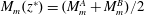 $M_{m}(z^{\ast })=(M_{m}^{A}+M_{m}^{B})/2$
, is marked ○. The time to which each profile corresponds is
$M_{m}(z^{\ast })=(M_{m}^{A}+M_{m}^{B})/2$
, is marked ○. The time to which each profile corresponds is
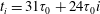 $t_{i}=31{\it\tau}_{0}+24{\it\tau}_{0}i$
, where
$t_{i}=31{\it\tau}_{0}+24{\it\tau}_{0}i$
, where
 $i=0\dots 3$
.
$i=0\dots 3$
.

The way in which the ambient flow field is affected by the unsteady jets is displayed in figure 9. Most noticeable is the divergence in the streamlines in the vicinity of negative longitudinal gradients of the momentum flux (i.e. regions in which
 $\partial _{z}M_{m}<0$
). This behaviour is consistent with the view that, for non-uniform velocity profiles,
$\partial _{z}M_{m}<0$
). This behaviour is consistent with the view that, for non-uniform velocity profiles,
 ${\it\alpha}_{disp1}$
leads to a reduction in entrainment (
${\it\alpha}_{disp1}$
leads to a reduction in entrainment (
 ${\it\alpha}_{disp1}<0$
), or relative divergence, when the flow decelerates in the longitudinal direction. On the other hand, in the region in figure 9(a) in which
${\it\alpha}_{disp1}<0$
), or relative divergence, when the flow decelerates in the longitudinal direction. On the other hand, in the region in figure 9(a) in which
 $\partial _{z}M_{m}>0$
, the behaviour of
$\partial _{z}M_{m}>0$
, the behaviour of
 ${\it\alpha}_{disp1}>0$
indicates an enhanced entrainment resulting from the acceleration of the jet in the longitudinal direction. When
${\it\alpha}_{disp1}>0$
indicates an enhanced entrainment resulting from the acceleration of the jet in the longitudinal direction. When
 $\partial _{z}M_{m}>0$
, both the spacing of the streamlines evident in figure 9(a) and the observation of an enhanced radial inflow reported by Borée et al. (Reference Borée, Atassi, Charnay and Taubert1997), support the qualitative predictions that can be obtained from the framework that was outlined in § 2.4. Indeed, we will demonstrate in Part 2 that if entrainment were not affected by
$\partial _{z}M_{m}>0$
, both the spacing of the streamlines evident in figure 9(a) and the observation of an enhanced radial inflow reported by Borée et al. (Reference Borée, Atassi, Charnay and Taubert1997), support the qualitative predictions that can be obtained from the framework that was outlined in § 2.4. Indeed, we will demonstrate in Part 2 that if entrainment were not affected by
 $\partial _{z}M_{m}$
, the local area
$\partial _{z}M_{m}$
, the local area
 $Q_{m}^{2}/M_{m}$
of the jet would necessarily increase or decease in order to accommodate the local deceleration (
$Q_{m}^{2}/M_{m}$
of the jet would necessarily increase or decease in order to accommodate the local deceleration (
 $\partial _{z}M_{m}<0$
) or acceleration (
$\partial _{z}M_{m}<0$
) or acceleration (
 $\partial _{z}M_{m}>0$
) of the flow, respectively.
$\partial _{z}M_{m}>0$
) of the flow, respectively.
Isolines of the stream function
 ${\it\psi}(r,z,t)$
at
${\it\psi}(r,z,t)$
at
 $t/{\it\tau}_{0}=64$
, where
$t/{\it\tau}_{0}=64$
, where
 $\overline{u}\equiv -r^{-1}\partial _{z}{\it\psi}$
and
$\overline{u}\equiv -r^{-1}\partial _{z}{\it\psi}$
and
 $\overline{w}\equiv r^{-1}\partial _{r}{\it\psi}$
, displayed alongside the normalised momentum flux.
$\overline{w}\equiv r^{-1}\partial _{r}{\it\psi}$
, displayed alongside the normalised momentum flux.

An advantage of examining entrainment via balances of mean momentum and energy in an unsteady jet is that it is not necessary to develop a storage model for the volume of the jet independently. Indeed, the area
 $Q_{m}^{2}/M_{m}$
is a statistical quantity that characterises the lateral spread of the jet rather than an observable physical threshold corresponding to a precise lateral extent. Consequently, as demonstrated in (2.23) and the previous paragraph, the entrainment properties of the unsteady jet can be inferred from the behaviour of
$Q_{m}^{2}/M_{m}$
is a statistical quantity that characterises the lateral spread of the jet rather than an observable physical threshold corresponding to a precise lateral extent. Consequently, as demonstrated in (2.23) and the previous paragraph, the entrainment properties of the unsteady jet can be inferred from the behaviour of
 $Q_{m}$
and
$Q_{m}$
and
 $M_{m}$
. By definition, at the upper limit
$M_{m}$
. By definition, at the upper limit
 $r_{d}$
of the integrals
$r_{d}$
of the integrals
 $Q_{m}$
and
$Q_{m}$
and
 $M_{m}$
, the longitudinal velocity
$M_{m}$
, the longitudinal velocity
 $\overline{w}(r_{d},z,t)$
is relatively small. Therefore, assuming that the unsteady flow remains slender, there will be a relatively small flux of momentum and energy at
$\overline{w}(r_{d},z,t)$
is relatively small. Therefore, assuming that the unsteady flow remains slender, there will be a relatively small flux of momentum and energy at
 $r=r_{d}$
. It is consequently not necessary to account for the effects of non-lateral entrainment in addition to the terms that already appear in (2.23). In situations in which the flow is not slender, or
$r=r_{d}$
. It is consequently not necessary to account for the effects of non-lateral entrainment in addition to the terms that already appear in (2.23). In situations in which the flow is not slender, or
 $\overline{w}(r_{d},z,t)$
is not relatively small, the entrainment relation (2.23) can be extended in a straightforward manner to account for longitudinal boundary fluxes.
$\overline{w}(r_{d},z,t)$
is not relatively small, the entrainment relation (2.23) can be extended in a straightforward manner to account for longitudinal boundary fluxes.
To track the location of the leading front,
 $z^{\ast }(t)$
, we use an intermediate value of the momentum flux to provide the implicit equation
$z^{\ast }(t)$
, we use an intermediate value of the momentum flux to provide the implicit equation
 $$\begin{eqnarray}M_{m}(z^{\ast })=\frac{M_{m}^{A}+M_{m}^{B}}{2},\end{eqnarray}$$
where
 $M_{m}^{B}$
and
$M_{m}^{B}$
and
 $M_{m}^{A}$
are constants, corresponding to the steady mean momentum fluxes before and after the step change, respectively. The front position is depicted in figure 8 with a circle. Figure 10(a,b) displays the relation
$M_{m}^{A}$
are constants, corresponding to the steady mean momentum fluxes before and after the step change, respectively. The front position is depicted in figure 8 with a circle. Figure 10(a,b) displays the relation
 $z^{\ast }(t)$
, determined numerically, and, with respect to the shaded isoregions of
$z^{\ast }(t)$
, determined numerically, and, with respect to the shaded isoregions of
 $\partial _{z}M_{m}$
, demonstrates that it coincides approximately with the inflection points in HL and LH, in addition to giving a smooth representation of the front position. Given the normalisation employed, the linear behaviour of the data in figure 10(c) reveals that the front position evolves according to
$\partial _{z}M_{m}$
, demonstrates that it coincides approximately with the inflection points in HL and LH, in addition to giving a smooth representation of the front position. Given the normalisation employed, the linear behaviour of the data in figure 10(c) reveals that the front position evolves according to
 $z^{\ast }\sim \sqrt{t}$
.
$z^{\ast }\sim \sqrt{t}$
.
Location of front
 $z^{\ast }(t)$
determined from simulation data. (a,b) Isoregions of
$z^{\ast }(t)$
determined from simulation data. (a,b) Isoregions of
 $\partial _{z}M_{m}$
, and a parabolic fit to the data shown with a bold line. The location of the asymptotic virtual source
$\partial _{z}M_{m}$
, and a parabolic fit to the data shown with a bold line. The location of the asymptotic virtual source
 $(z_{v},t_{v})$
is marked
$(z_{v},t_{v})$
is marked
 $\times$
. (c) The front position with respect to a quadratically scaled longitudinal axis, in addition to the theoretical location of the front when the longitudinal velocity is assumed to have a top-hat form (
$\times$
. (c) The front position with respect to a quadratically scaled longitudinal axis, in addition to the theoretical location of the front when the longitudinal velocity is assumed to have a top-hat form (
 ${\it\lambda}^{\ast }=1$
) and a Gaussian form (
${\it\lambda}^{\ast }=1$
) and a Gaussian form (
 ${\it\lambda}^{\ast }=2$
).
${\it\lambda}^{\ast }=2$
).

The scaling observed in figure 10 can be interpreted by assuming that the front propagates at a rate given by
 $$\begin{eqnarray}\frac{\text{d}z^{\ast }}{\text{d}t}={\it\lambda}^{\ast }\frac{M_{m}^{\ast 1/2}}{2{\it\alpha}_{0}(z^{\ast }-z_{v})},\end{eqnarray}$$
where
 $M_{m}^{\ast }$
is a suitable constant momentum flux, characteristic of the motion at the leading edge of the front, and
$M_{m}^{\ast }$
is a suitable constant momentum flux, characteristic of the motion at the leading edge of the front, and
 ${\it\lambda}^{\ast }$
is a constant, which in § 5.1 we show can be interpreted as an eigenvalue of the system. In fact, under certain simplifying assumptions that will be discussed in Part 2, the appropriate momentum flux
${\it\lambda}^{\ast }$
is a constant, which in § 5.1 we show can be interpreted as an eigenvalue of the system. In fact, under certain simplifying assumptions that will be discussed in Part 2, the appropriate momentum flux
 $M_{m}^{\ast }$
can be obtained exactly according to
$M_{m}^{\ast }$
can be obtained exactly according to
 $$\begin{eqnarray}M_{m}^{\ast }=\frac{1}{4}\left(\frac{M_{m}^{A}-M_{m}^{B}}{M_{m}^{A\,1/2}-M_{m}^{B\,1/2}}\right)^{2},\end{eqnarray}$$
when the front is regarded as a shock (see e.g. Toro Reference Toro1997). Integration of (4.5) reveals that
 $$\begin{eqnarray}(z^{\ast }-z_{v})^{2}=\frac{{\it\lambda}^{\ast }M_{m}^{\ast 1/2}}{{\it\alpha}_{0}}(t-t_{v}),\end{eqnarray}$$
where
 $t_{v}$
is a constant of integration that corresponds to the location of an asymptotic virtual source in time. Equation (4.7) describes the scaling observed in figure 10 and, with (4.6), provides a normalisation for fronts of different strengths. A similar argument was used by Abraham (Reference Abraham1996) to deduce that the total mass entrained into an unsteady gas jet has a cubic dependence on its longitudinal penetration. Observable in figure 10 is that
$t_{v}$
is a constant of integration that corresponds to the location of an asymptotic virtual source in time. Equation (4.7) describes the scaling observed in figure 10 and, with (4.6), provides a normalisation for fronts of different strengths. A similar argument was used by Abraham (Reference Abraham1996) to deduce that the total mass entrained into an unsteady gas jet has a cubic dependence on its longitudinal penetration. Observable in figure 10 is that
 ${\it\lambda}^{\ast }\approx 2$
in both simulations, which suggests that the front propagates at
${\it\lambda}^{\ast }\approx 2$
in both simulations, which suggests that the front propagates at
 $2w_{m}$
rather than
$2w_{m}$
rather than
 $w_{m}$
. For Gaussian profiles
$w_{m}$
. For Gaussian profiles
 $2w_{m}$
corresponds to the maximum velocity whilst
$2w_{m}$
corresponds to the maximum velocity whilst
 $w_{m}$
corresponds to the mean velocity. In the next section we will look at the hyperbolic character of the governing equations in greater detail and show that the eigenvalue
$w_{m}$
corresponds to the mean velocity. In the next section we will look at the hyperbolic character of the governing equations in greater detail and show that the eigenvalue
 ${\it\lambda}^{\ast }$
can be inferred with reasonable accuracy using the steady-state data. In doing so we will be able to demonstrate that it is the velocity profile of the jet that is chiefly responsible for determining the propagation speed of the front.
${\it\lambda}^{\ast }$
can be inferred with reasonable accuracy using the steady-state data. In doing so we will be able to demonstrate that it is the velocity profile of the jet that is chiefly responsible for determining the propagation speed of the front.
In figure 11 the momentum flux over the time interval
 $[63,159]{\it\tau}_{0}$
is plotted with respect to a similarity variable obtained by rescaling the longitudinal coordinate by the observed front position
$[63,159]{\it\tau}_{0}$
is plotted with respect to a similarity variable obtained by rescaling the longitudinal coordinate by the observed front position
 $z^{\ast }(t)$
. The observable collapse of the data confirms that the length scale associated with the spread of the front scales in proportion to
$z^{\ast }(t)$
. The observable collapse of the data confirms that the length scale associated with the spread of the front scales in proportion to
 $z^{\ast }(t)$
. In turn, one can infer that the processes responsible for the mixing of the front scales according to the local integral properties of the jet, rather than an independent scale. The picture that emerges in physical coordinates is similar to the cap of the starting plume envisaged by Turner (Reference Turner1962): for all times the longitudinal extent of the front remains in constant proportion to the local radius of the jet
$z^{\ast }(t)$
. In turn, one can infer that the processes responsible for the mixing of the front scales according to the local integral properties of the jet, rather than an independent scale. The picture that emerges in physical coordinates is similar to the cap of the starting plume envisaged by Turner (Reference Turner1962): for all times the longitudinal extent of the front remains in constant proportion to the local radius of the jet
 $r_{m}(z^{\ast }(t),t)$
. It is interesting that for jets the observed, and indeed expected, scaling
$r_{m}(z^{\ast }(t),t)$
. It is interesting that for jets the observed, and indeed expected, scaling
 $z^{\ast }(t)\sim \sqrt{t}$
corresponds to one of classical dispersion (Taylor Reference Taylor1953). The self-similarity evident in figure 11 suggests that unsteady jets attain an equilibrium state. In this state one expects the dynamics of the front to be invariant with time, provided that all quantities are non-dimensionalised using the local scales
$z^{\ast }(t)\sim \sqrt{t}$
corresponds to one of classical dispersion (Taylor Reference Taylor1953). The self-similarity evident in figure 11 suggests that unsteady jets attain an equilibrium state. In this state one expects the dynamics of the front to be invariant with time, provided that all quantities are non-dimensionalised using the local scales
 $w_{m}(z,t)$
and
$w_{m}(z,t)$
and
 $r_{m}(z,t)$
. This kind of self-similarity is weaker than the similarity that one finds in steady jets, because it does not imply that the radial dependence of
$r_{m}(z,t)$
. This kind of self-similarity is weaker than the similarity that one finds in steady jets, because it does not imply that the radial dependence of
 $\overline{w}/w_{m}$
is everywhere the same. Furthermore, one would not expect to find similarity in the near field. Indeed, near-field (i.e. small-time) effects are evident in figure 11 as regions in which the data do not collapse. It is natural to expect that an unsteady jet produced by any change in source conditions that takes place over a finite time will eventually attain a state of similarity such that
$\overline{w}/w_{m}$
is everywhere the same. Furthermore, one would not expect to find similarity in the near field. Indeed, near-field (i.e. small-time) effects are evident in figure 11 as regions in which the data do not collapse. It is natural to expect that an unsteady jet produced by any change in source conditions that takes place over a finite time will eventually attain a state of similarity such that
 $$\begin{eqnarray}\frac{\overline{w}}{w_{m}}=f\left(\frac{r}{r_{m}},\frac{z^{2}{\it\alpha}_{0}}{M_{m}^{\ast 1/2}t},\frac{M_{m}^{A}}{M_{m}^{B}}\right).\end{eqnarray}$$
In converging to such a state, longitudinal mixing will ensure that the jet has a progressively weaker dependence on the precise way in which its source conditions were changed.
Self-similarity of the simulation results for the momentum flux
 $M_{m}$
over the time interval [63, 159]
$M_{m}$
over the time interval [63, 159]
 ${\it\tau}_{0}$
compared to a similarity solution of a corresponding linear advection–dispersion equation.
${\it\tau}_{0}$
compared to a similarity solution of a corresponding linear advection–dispersion equation.
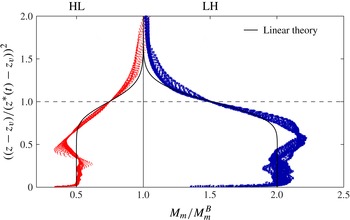
5. Theory of the front
In this section we analyse the propagation speed and spreading rate of the front in greater detail. We will show that the former is determined by the values of the dimensionless fluxes
 ${\it\gamma}_{g}$
and
${\it\gamma}_{g}$
and
 ${\it\beta}_{g}$
, and is significantly influenced by the steady-state longitudinal velocity profile. Mixing of the front, in contrast, requires that the dimensionless fluxes
${\it\beta}_{g}$
, and is significantly influenced by the steady-state longitudinal velocity profile. Mixing of the front, in contrast, requires that the dimensionless fluxes
 ${\it\gamma}_{g}$
and/or
${\it\gamma}_{g}$
and/or
 ${\it\beta}_{g}$
depart from their steady-state values, which implies a local departure from similarity in the jet. We distinguish these effects by identifying them as type I and type II dispersion, respectively.
${\it\beta}_{g}$
depart from their steady-state values, which implies a local departure from similarity in the jet. We distinguish these effects by identifying them as type I and type II dispersion, respectively.
5.1. Type I dispersion and characteristic curves
Here we will determine the characteristic curves of the system (2.12) and (2.13) in the general case, for which it will be assumed that the rates with which energy and momentum are transported are different, i.e.
 ${\it\gamma}_{g}\neq {\it\beta}_{g}$
. Using the momentum–energy formulation we express the governing equation for unsteady jets as
${\it\gamma}_{g}\neq {\it\beta}_{g}$
. Using the momentum–energy formulation we express the governing equation for unsteady jets as
 $$\begin{eqnarray}\frac{\partial }{\partial t}\left(\begin{array}{@{}c@{}}Q_{m}\\ M_{m}\end{array}\right)+\left[\begin{array}{@{}cc@{}}0 & {\it\beta}_{g}\\ -{\it\gamma}_{g}{\displaystyle \frac{M_{m}^{2}}{Q_{m}^{2}}} & 2{\it\gamma}_{g}{\displaystyle \frac{M_{m}}{Q_{m}}}\end{array}\right]\frac{\partial }{\partial z}\left(\begin{array}{@{}c@{}}Q_{m}\\ M_{m}\end{array}\right)=\left(\begin{array}{@{}c@{}}0\\ {\it\delta}_{g}{\displaystyle \frac{M_{m}^{5/2}}{Q_{m}^{2}}}\end{array}\right).\end{eqnarray}$$
Looking locally, we assume that the dimensionless terms
 ${\it\beta}_{g},{\it\gamma}_{g}$
and
${\it\beta}_{g},{\it\gamma}_{g}$
and
 ${\it\delta}_{g}$
are constants, thereby restricting analysis to type I dispersion. This allows us to understand, to leading order, the effect that they have on the classification of the system. Characteristic surfaces, on which a function
${\it\delta}_{g}$
are constants, thereby restricting analysis to type I dispersion. This allows us to understand, to leading order, the effect that they have on the classification of the system. Characteristic surfaces, on which a function
 ${\it\Phi}(z,t)$
is constant, satisfy the following condition:
${\it\Phi}(z,t)$
is constant, satisfy the following condition:
 $$\begin{eqnarray}\det \left[\begin{array}{@{}cc@{}}-{\it\lambda}^{\ast } & {\it\beta}_{g}{\displaystyle \frac{Q_{m}}{M_{m}}}\\ -{\it\gamma}_{g}{\displaystyle \frac{M_{m}}{Q_{m}}} & 2{\it\gamma}_{g}-{\it\lambda}^{\ast }\end{array}\right]=0,\end{eqnarray}$$
where the eigenvalue
 ${\it\lambda}^{\ast }$
represents a dimensionless velocity defined by
${\it\lambda}^{\ast }$
represents a dimensionless velocity defined by
 $$\begin{eqnarray}{\it\lambda}^{\ast }\equiv \frac{\text{d}z}{\text{d}t}\frac{Q_{m}}{M_{m}}=-\frac{\partial {\it\Phi}}{\partial t}\left(\frac{\partial {\it\Phi}}{\partial z}\right)^{-1}\frac{Q_{m}}{M_{m}}.\end{eqnarray}$$
The relation (5.2) implies that
 $$\begin{eqnarray}{\it\lambda}^{\ast }={\it\gamma}_{g}\left(1\pm \sqrt{1-{\displaystyle \frac{{\it\beta}_{g}}{{\it\gamma}_{g}}}}\right).\end{eqnarray}$$
In the eigenvalues (5.4) we see that when the rates with which momentum and energy are transported are equal (i.e. when
 ${\it\beta}_{g}={\it\gamma}_{g}$
) the eigenvalues, and therefore the characteristic curves, overlap. In that case it can be shown that the eigenvectors of the system are not linearly independent and the system is parabolic (see e.g. Whitham Reference Whitham1974). Indeed, it is a parabolic form of the equations that is implied by the top-hat model of Scase et al. (Reference Scase, Caulfield, Dalziel and Hunt2006). However, substitution of the values of
${\it\beta}_{g}={\it\gamma}_{g}$
) the eigenvalues, and therefore the characteristic curves, overlap. In that case it can be shown that the eigenvectors of the system are not linearly independent and the system is parabolic (see e.g. Whitham Reference Whitham1974). Indeed, it is a parabolic form of the equations that is implied by the top-hat model of Scase et al. (Reference Scase, Caulfield, Dalziel and Hunt2006). However, substitution of the values of
 ${\it\gamma}_{g}$
and
${\it\gamma}_{g}$
and
 ${\it\beta}_{g}$
obtained from the steady state (see table 2) suggests that
${\it\beta}_{g}$
obtained from the steady state (see table 2) suggests that
 $$\begin{eqnarray}{\it\lambda}^{\ast }\approx 1.4\pm 0.7,\end{eqnarray}$$
and therefore that the system is hyperbolic. Unlike parabolic systems, in hyperbolic systems fast-propagating disturbances can overtake slower disturbances. Indeed, there is a close analogy between the unsteady jet equations and the shallow-water equations for supercritical flow. In both cases there are generally two families of characteristic curves and information is only able to travel downstream.
The characteristic curves are paths along which the total derivatives of several quasi-invariant quantities are decoupled. Using the eigenvectors of the system, the invariants are defined in terms of the total derivatives:
 $$\begin{eqnarray}\text{d}Y_{m}=-\frac{{\it\gamma}_{g}}{{\it\lambda}^{\ast }}\frac{M_{m}}{Q_{m}}Q_{m}^{-{\it\gamma}_{g}/{\it\lambda}^{\ast }}\text{d}Q_{m}+Q_{m}^{-{\it\gamma}_{g}/{\it\lambda}^{\ast }}\text{d}M_{m},\end{eqnarray}$$
where the integrating factor
 $Q_{m}^{-{\it\gamma}_{g}/{\it\lambda}^{\ast }}$
has been introduced. The quasi-invariants are therefore found to be
$Q_{m}^{-{\it\gamma}_{g}/{\it\lambda}^{\ast }}$
has been introduced. The quasi-invariants are therefore found to be
 $$\begin{eqnarray}Y_{m}=M_{m}Q_{m}^{-{\it\gamma}_{g}/{\it\lambda}^{\ast }},\end{eqnarray}$$
to within a constant factor. We note that when the system is parabolic and
 ${\it\lambda}^{\ast }=1$
, the quasi-invariants are identical and equal to
${\it\lambda}^{\ast }=1$
, the quasi-invariants are identical and equal to
 $M_{m}/Q_{m}=w_{m}$
. Along the characteristic curves the governing equations become
$M_{m}/Q_{m}=w_{m}$
. Along the characteristic curves the governing equations become
 $$\begin{eqnarray}\frac{\text{d}Y_{m}}{\text{d}t}={\it\delta}_{g}\frac{M_{m}^{5/2}}{Q_{m}^{2+{\it\gamma}_{g}/{\it\lambda}^{\ast }}}.\end{eqnarray}$$
The quasi-invariants prove particularly useful in understanding the behaviour of the area of the jet
 $A_{m}$
. It can be shown that along fast and slow characteristic curves emanating from an instantaneous change in
$A_{m}$
. It can be shown that along fast and slow characteristic curves emanating from an instantaneous change in
 $M_{m}$
, the area retains its steady-state form,
$M_{m}$
, the area retains its steady-state form,
 $A_{m}=4{\it\alpha}_{0}^{2}z^{2}$
. In Part 2 we show that the behaviour of the area between these curves depends on their separation, i.e. on the discriminant
$A_{m}=4{\it\alpha}_{0}^{2}z^{2}$
. In Part 2 we show that the behaviour of the area between these curves depends on their separation, i.e. on the discriminant
 $1-{\it\beta}_{g}/{\it\gamma}_{g}$
, for which there exists a distinguished value that renders the area insensitive to changes in
$1-{\it\beta}_{g}/{\it\gamma}_{g}$
, for which there exists a distinguished value that renders the area insensitive to changes in
 $Q_{m}$
and
$Q_{m}$
and
 $M_{m}$
. Thus, there exists a value of
$M_{m}$
. Thus, there exists a value of
 $1-{\it\beta}_{g}/{\it\gamma}_{g}$
that ensures straight-sidedness in the jet for all time. Remarkably, this value is obtained when the jet is assumed to have a Gaussian form, with
$1-{\it\beta}_{g}/{\it\gamma}_{g}$
that ensures straight-sidedness in the jet for all time. Remarkably, this value is obtained when the jet is assumed to have a Gaussian form, with
 ${\it\beta}_{g}=1$
and
${\it\beta}_{g}=1$
and
 ${\it\gamma}_{g}=4/3$
.
${\it\gamma}_{g}=4/3$
.
5.2. Type II dispersion and front mixing
In the previous section we established type I dispersion under the assumption that
 ${\it\beta}_{g}$
and
${\it\beta}_{g}$
and
 ${\it\gamma}_{g}$
are constants, equal to their steady-state values. However, such an assumption is unrealistic in the vicinity of a steep front where self-similarity will, in general, not be maintained. This naturally raises the question of what effect a departure from self-similarity will have on the local fluxes and, therefore, on the longitudinal mixing at the front. Indeed, in § 4.3 a non-negligible longitudinal spreading of the front was observed, which was found to scale according to
${\it\gamma}_{g}$
are constants, equal to their steady-state values. However, such an assumption is unrealistic in the vicinity of a steep front where self-similarity will, in general, not be maintained. This naturally raises the question of what effect a departure from self-similarity will have on the local fluxes and, therefore, on the longitudinal mixing at the front. Indeed, in § 4.3 a non-negligible longitudinal spreading of the front was observed, which was found to scale according to
 $\sqrt{t}$
. In this section we begin by estimating the mixing coefficient associated with the observed longitudinal spreading rate, before looking at the local variations in the dimensionless fluxes in the jet.
$\sqrt{t}$
. In this section we begin by estimating the mixing coefficient associated with the observed longitudinal spreading rate, before looking at the local variations in the dimensionless fluxes in the jet.
The spread of the front can be obtained by assuming that the process can be described by an advection–dispersion equation of the form
 $$\begin{eqnarray}\frac{\partial M_{m}}{\partial t}+{\it\lambda}^{\ast }\frac{M_{m}^{\ast 1/2}}{2{\it\alpha}_{0}(z-z_{v})}\frac{\partial M_{m}}{\partial z}=D_{e}\frac{\partial ^{2}M_{m}}{\partial z^{2}}.\end{eqnarray}$$
Equation (5.9) can be expressed as an ordinary differential equation (see appendix B) using the similarity scaling that was observed in § 4.3. An estimation of the dispersion coefficient
 $D_{e}$
can be obtained by matching the similarity solution to the data displayed in figure 11. Specifically, the matching is performed by comparing the gradient of the similarity solution at the level of the front to that observed in the transformed simulation data. To do this we average over each of the instantaneous profiles comprising figure 11. To quantify mixing effects, rather than the spreading resulting from the rarefaction behaviour of HL, we use LH for our estimation. The gradient of the similarity solution of (5.9) was obtained to leading order by assuming that the effects of longitudinal mixing are relatively weak compared to the advection of the front, as described in appendix B. This procedure suggests that
$D_{e}$
can be obtained by matching the similarity solution to the data displayed in figure 11. Specifically, the matching is performed by comparing the gradient of the similarity solution at the level of the front to that observed in the transformed simulation data. To do this we average over each of the instantaneous profiles comprising figure 11. To quantify mixing effects, rather than the spreading resulting from the rarefaction behaviour of HL, we use LH for our estimation. The gradient of the similarity solution of (5.9) was obtained to leading order by assuming that the effects of longitudinal mixing are relatively weak compared to the advection of the front, as described in appendix B. This procedure suggests that
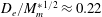 $D_{e}/M_{m}^{\ast \,1/2}\approx 0.22$
, which defines the similarity solution that is shown in figure 11 with a solid line. Referring back to § 3, it should be noted that in theory the relatively small, yet finite, time interval
$D_{e}/M_{m}^{\ast \,1/2}\approx 0.22$
, which defines the similarity solution that is shown in figure 11 with a solid line. Referring back to § 3, it should be noted that in theory the relatively small, yet finite, time interval
 ${\it\delta}t<2{\it\tau}_{0}$
over which we average the data is responsible for a small amount of smoothing over the longitudinal direction. However, this contribution scales according to
${\it\delta}t<2{\it\tau}_{0}$
over which we average the data is responsible for a small amount of smoothing over the longitudinal direction. However, this contribution scales according to
 ${\it\delta}t^{2}/t^{2}$
, whose value is no greater than
${\it\delta}t^{2}/t^{2}$
, whose value is no greater than
 $2\times 10^{-4}$
for the data presented in figure 11, from which the value of
$2\times 10^{-4}$
for the data presented in figure 11, from which the value of
 $D_{e}$
was inferred. Accounting for the observed steepness of the front, we estimate that our inferred value of
$D_{e}$
was inferred. Accounting for the observed steepness of the front, we estimate that our inferred value of
 $D_{e}$
overestimates the actual longitudinal mixing coefficient due to time averaging by not more than 1 %. Figure 11 reveals that (5.9) provides a reasonably accurate first approximation to the front in each case. An interesting aspect of this result is that (5.9) ignores the coupling that exists between
$D_{e}$
overestimates the actual longitudinal mixing coefficient due to time averaging by not more than 1 %. Figure 11 reveals that (5.9) provides a reasonably accurate first approximation to the front in each case. An interesting aspect of this result is that (5.9) ignores the coupling that exists between
 $Q_{m}$
and
$Q_{m}$
and
 $M_{m}$
. In Part 2 we will account for the surprising effectiveness of (5.9), and show that it implies that unsteady jets remain approximately straight-sided.
$M_{m}$
. In Part 2 we will account for the surprising effectiveness of (5.9), and show that it implies that unsteady jets remain approximately straight-sided.
Having obtained an estimation for
 $D_{e}$
, the logical next step is to ascertain whether the longitudinal mixing is due to turbulence or shear-flow dispersion of the kind identified by Taylor (Reference Taylor1953). Shear-flow dispersion is caused by lateral gradients in the mean longitudinal velocity acting over longitudinal gradients of a transported variable. As discovered by Taylor (Reference Taylor1953), dispersion produces a local deformation in the radial dependence of the transported quantity, which, owing to its correlation with a non-uniform velocity can enhance or diminish the total flux of the quantity.
$D_{e}$
, the logical next step is to ascertain whether the longitudinal mixing is due to turbulence or shear-flow dispersion of the kind identified by Taylor (Reference Taylor1953). Shear-flow dispersion is caused by lateral gradients in the mean longitudinal velocity acting over longitudinal gradients of a transported variable. As discovered by Taylor (Reference Taylor1953), dispersion produces a local deformation in the radial dependence of the transported quantity, which, owing to its correlation with a non-uniform velocity can enhance or diminish the total flux of the quantity.
We make an estimation of the average turbulence eddy viscosity
 ${\it\nu}_{Tm}$
using the gradient diffusion hypothesis:
${\it\nu}_{Tm}$
using the gradient diffusion hypothesis:
 $$\begin{eqnarray}\overline{u^{\prime }w^{\prime }}=-{\it\nu}_{Tm}\frac{\partial \overline{w}}{\partial r},\end{eqnarray}$$
and evaluate the dominant production term by assuming that
 $\overline{w}$
follows a Gaussian distribution (2.19):
$\overline{w}$
follows a Gaussian distribution (2.19):
 $$\begin{eqnarray}P_{m}\equiv 4\int _{0}^{\infty }\overline{u^{\prime }w^{\prime }}\frac{\partial \overline{w}}{\partial r}r\text{d}r=-4{\it\nu}_{Tm}\int _{0}^{\infty }\left(\frac{\partial \overline{w}}{\partial r}\right)^{2}r\text{d}r=-8{\it\nu}_{Tm}w_{m}^{2}.\end{eqnarray}$$
On using the definition of
 ${\it\delta}_{m}$
and the relation
${\it\delta}_{m}$
and the relation
 ${\it\delta}_{m}=-2{\it\alpha}_{0}{\it\gamma}_{m}$
, implied by (2.24), to relate
${\it\delta}_{m}=-2{\it\alpha}_{0}{\it\gamma}_{m}$
, implied by (2.24), to relate
 $P_{m}$
to
$P_{m}$
to
 ${\it\alpha}_{0}$
, we find
${\it\alpha}_{0}$
, we find
 $$\begin{eqnarray}{\it\nu}_{Tm}=\frac{{\it\alpha}_{0}}{3}M_{m}^{\ast \,1/2}.\end{eqnarray}$$
The observed dispersion coefficient
 $D_{e}$
is several times larger than the eddy viscosity
$D_{e}$
is several times larger than the eddy viscosity
 ${\it\nu}_{Tm}$
; indeed
${\it\nu}_{Tm}$
; indeed
 $D_{e}/M_{m}^{\ast \,1/2}=0.22$
compared to
$D_{e}/M_{m}^{\ast \,1/2}=0.22$
compared to
 ${\it\nu}_{Tm}/M_{m}^{\ast \,1/2}=0.023$
. Although the estimation (5.12) does not account for the fact that
${\it\nu}_{Tm}/M_{m}^{\ast \,1/2}=0.023$
. Although the estimation (5.12) does not account for the fact that
 ${\it\nu}_{Tm}$
might change locally at the front, its value relative to
${\it\nu}_{Tm}$
might change locally at the front, its value relative to
 $D_{e}$
suggests that the mixing of the front is primarily a dispersive phenomenon. In Part 2 we address how the mixing of the front can be described using a simple model for dispersion based on the approach proposed by Taylor (Reference Taylor1953, Reference Taylor1954).
$D_{e}$
suggests that the mixing of the front is primarily a dispersive phenomenon. In Part 2 we address how the mixing of the front can be described using a simple model for dispersion based on the approach proposed by Taylor (Reference Taylor1953, Reference Taylor1954).
We are now in a position to address the origin of the longitudinal mixing observed in figure 11. In § 5.1 we assumed that
 ${\it\gamma}_{g}$
remains constant in the vicinity of a front. This amounts to assuming that the self-similarity of the jet is unaffected by a shock or rarefaction, which, from a physical point of view, is unrealistic. In fact, unless the velocity profiles have a top-hat form, we expect that non-uniform profiles of velocity will redistribute energy in the longitudinal direction and therefore smooth steep fronts. This behaviour is confirmed in figure 12, which displays a moving average of the dimensionless mean (a) and dimensionless turbulence (b) longitudinal kinetic energy relative to steady-state profiles. Positive (negative) values indicate parts of the flow where the mean or turbulence energy is higher (lower) than the steady-state value at the same location. In LH the negative longitudinal gradient in
${\it\gamma}_{g}$
remains constant in the vicinity of a front. This amounts to assuming that the self-similarity of the jet is unaffected by a shock or rarefaction, which, from a physical point of view, is unrealistic. In fact, unless the velocity profiles have a top-hat form, we expect that non-uniform profiles of velocity will redistribute energy in the longitudinal direction and therefore smooth steep fronts. This behaviour is confirmed in figure 12, which displays a moving average of the dimensionless mean (a) and dimensionless turbulence (b) longitudinal kinetic energy relative to steady-state profiles. Positive (negative) values indicate parts of the flow where the mean or turbulence energy is higher (lower) than the steady-state value at the same location. In LH the negative longitudinal gradient in
 $M_{m}$
at the front means that fluid of relatively high energy, transported from behind the front, is concentrated on the axis of the jet and surrounded by fluid of relatively low energy. In HL, in which the longitudinal gradient in
$M_{m}$
at the front means that fluid of relatively high energy, transported from behind the front, is concentrated on the axis of the jet and surrounded by fluid of relatively low energy. In HL, in which the longitudinal gradient in
 $M_{m}$
is positive, the situation is reversed and fluid with relatively high energy is removed from the axis of the jet at the front. It is notable that the deformation of both the mean energy profile and the turbulence energy profile has a similar form.
$M_{m}$
is positive, the situation is reversed and fluid with relatively high energy is removed from the axis of the jet at the front. It is notable that the deformation of both the mean energy profile and the turbulence energy profile has a similar form.
Moving averages (following the front), relative to steady-state profiles. (a) Normalised longitudinal mean kinetic energy profile and (b) longitudinal turbulence kinetic energy. Steady-state profiles were obtained by averaging profiles in both L and H over the range
 $z/r_{0}\in [28,55]$
.
$z/r_{0}\in [28,55]$
.

The moving average of the dimensionless fluxes displayed in figure 13 confirms that both
 ${\it\gamma}_{m}$
and
${\it\gamma}_{m}$
and
 ${\it\gamma}_{f}$
increase in LH and decrease in HL in the vicinity of the front. Noteworthy is the fact that in spite of the departures from steady-state similarity observable in
${\it\gamma}_{f}$
increase in LH and decrease in HL in the vicinity of the front. Noteworthy is the fact that in spite of the departures from steady-state similarity observable in
 $\overline{w^{\prime 2}}$
in figure 12, figure 13 shows that the dimensionless turbulent transport
$\overline{w^{\prime 2}}$
in figure 12, figure 13 shows that the dimensionless turbulent transport
 ${\it\beta}_{f}$
is not significantly affected by the front. To appreciate this, note that the deviation from self-similarity of
${\it\beta}_{f}$
is not significantly affected by the front. To appreciate this, note that the deviation from self-similarity of
 $\overline{w^{\prime 2}}$
shown in figure 12 appears in a product with
$\overline{w^{\prime 2}}$
shown in figure 12 appears in a product with
 $r$
when integrated over the jet to give
$r$
when integrated over the jet to give
 ${\it\beta}_{f}$
. The dispersion described in the previous paragraph arises due to the redistribution of a quantity over the radius of the jet, rather than a change in the area integral of that quantity. Such effects belong exclusively to the mean energy equation, because there, unlike in the momentum equation, the quantities appear in a product with
${\it\beta}_{f}$
. The dispersion described in the previous paragraph arises due to the redistribution of a quantity over the radius of the jet, rather than a change in the area integral of that quantity. Such effects belong exclusively to the mean energy equation, because there, unlike in the momentum equation, the quantities appear in a product with
 $\overline{w}$
. In particular, the parameter describing dispersion in
$\overline{w}$
. In particular, the parameter describing dispersion in
 $\overline{w}\overline{w^{\prime 2}}$
is
$\overline{w}\overline{w^{\prime 2}}$
is
 ${\it\gamma}_{f}-2{\it\beta}_{f}$
(see § 2), and has a behaviour that is similar to
${\it\gamma}_{f}-2{\it\beta}_{f}$
(see § 2), and has a behaviour that is similar to
 ${\it\gamma}_{m}-1$
in the vicinity of the front in LH. We also note that the significant increase in
${\it\gamma}_{m}-1$
in the vicinity of the front in LH. We also note that the significant increase in
 ${\it\gamma}_{m}$
in HL upstream of the front (see bottom of figure 13
a) is coincident with the trough in
${\it\gamma}_{m}$
in HL upstream of the front (see bottom of figure 13
a) is coincident with the trough in
 $M_{m}$
that develops slightly ahead of the secondary, slower front (see also figure 8), whose dynamics is beyond the scope of the present investigation.
$M_{m}$
that develops slightly ahead of the secondary, slower front (see also figure 8), whose dynamics is beyond the scope of the present investigation.
Moving average of energy flux parameters, at the level of the front. Dashed lines correspond to the average parameter values from the steady data, reported in § 4.2.

6. Conclusions
In this paper we have presented results from the direct simulation of steady and unsteady jets. To inspect the results we developed an unsteady momentum–energy framework that provides a logical generalisation, in the absence of buoyancy, of the approach employed by Priestley & Ball (Reference Priestley and Ball1955) and Kaminski et al. (Reference Kaminski, Tait and Carazzo2005). Using the framework in a diagnostic capacity, we reported the value of several dimensionless transport and turbulence production parameters in a steady jet, which prove useful in understanding the behaviour of unsteady jets. In particular, we observed that the propagation speed of a front is approximately equal to
 ${\it\lambda}^{\ast }w_{m}^{\ast }$
, where
${\it\lambda}^{\ast }w_{m}^{\ast }$
, where
 ${\it\lambda}^{\ast }\approx 2$
and
${\it\lambda}^{\ast }\approx 2$
and
 $w_{m}^{\ast }\equiv M_{m}^{\ast }/2{\it\alpha}_{0}z$
is a top-hat velocity that characterises the motion at the front (see figure 10). Following relatively small changes in
$w_{m}^{\ast }\equiv M_{m}^{\ast }/2{\it\alpha}_{0}z$
is a top-hat velocity that characterises the motion at the front (see figure 10). Following relatively small changes in
 $M_{m}$
at the source, we have
$M_{m}$
at the source, we have
 $M_{m}^{\ast }\approx M_{m}$
, and the front’s propagation speed will be
$M_{m}^{\ast }\approx M_{m}$
, and the front’s propagation speed will be
 $2w_{m}$
, which, for Gaussian profiles, is equal to the velocity on the axis of the jet. In addition, we observed that the behaviour of the front accords with a self-similar process (see figure 11), whose position and longitudinal extent scales according to
$2w_{m}$
, which, for Gaussian profiles, is equal to the velocity on the axis of the jet. In addition, we observed that the behaviour of the front accords with a self-similar process (see figure 11), whose position and longitudinal extent scales according to
 $z^{\ast }\sim \sqrt{t}$
. This allowed us to determine the longitudinal spreading rate of the front using a similarity transformation (appendix B) and, consequently, a mixing coefficient
$z^{\ast }\sim \sqrt{t}$
. This allowed us to determine the longitudinal spreading rate of the front using a similarity transformation (appendix B) and, consequently, a mixing coefficient
 $D_{e}$
. By comparing
$D_{e}$
. By comparing
 $D_{e}$
to the typical magnitude of the eddy viscosity it was demonstrated that the mixing is primarily due to dispersion.
$D_{e}$
to the typical magnitude of the eddy viscosity it was demonstrated that the mixing is primarily due to dispersion.
The notion of energy dispersion unifies several distinct concepts that are prevalent in the behaviour of unsteady jets. In this regard, type I dispersion results from non-uniform profiles of velocity that remain self-similar with height. Under such conditions the profile of kinetic energy is narrower than the profile of velocity, which means that the dimensionless energy flux is greater than the dimensionless momentum flux. In turn, this gives the resulting integral equations a hyperbolic character. In Part 2, we will show that type I dispersion determines the behaviour of the area of the jet in the vicinity of a front and the rate at which perturbations at the source grow or decay in the longitudinal direction. Type II dispersion, in contrast, concerns departures from self-similarity that modify the local fluxes, and was shown to be chiefly responsible for the longitudinal mixing in the unsteady jets. In addition, type II dispersion provides the only way in which the area of the jet can be mixed in the longitudinal direction. Both type I and type II dispersion reside in the mean energy equation.
Dispersion in jets can account for highly influential transport processes in terms of mean flow properties alone, without explicit reference to turbulence terms. More precisely, in the present context turbulence can be viewed as a process that inhibits dispersion in the way that Taylor (Reference Taylor1954) made evident for pipe flow. Longitudinal mixing by dispersion includes the effects of turbulence implicitly and, by focusing on the properties of the mean flow, sits comfortably with the established treatment of jets and plumes. Moreover, in keeping with Taylor dispersion, it is the Reynolds stress,
 $\overline{u^{\prime }w^{\prime }}$
, which determines the steady-state entrainment, that continues to play a dominant role. However, the present study has not examined the effect that a step change in momentum flux has on the turbulence kinetic energy budget. In particular, the behaviour of the turbulence production is an area that would benefit from further attention (see e.g. Borée et al.
Reference Borée, Atassi, Charnay and Taubert1997) and could be analysed from an integral perspective using the framework that we described in § 2. In Part 2 of this work we will produce a simple closure for unsteady jets based on Taylor dispersion.
$\overline{u^{\prime }w^{\prime }}$
, which determines the steady-state entrainment, that continues to play a dominant role. However, the present study has not examined the effect that a step change in momentum flux has on the turbulence kinetic energy budget. In particular, the behaviour of the turbulence production is an area that would benefit from further attention (see e.g. Borée et al.
Reference Borée, Atassi, Charnay and Taubert1997) and could be analysed from an integral perspective using the framework that we described in § 2. In Part 2 of this work we will produce a simple closure for unsteady jets based on Taylor dispersion.
Acknowledgements
The authors wish to express their gratitude for the High Performance Computing resource at Imperial College London and would like to thank the UK Turbulence Consortium for their support under grant number EP/L000261/1. In addition, J.C. gratefully acknowledges funding from the Engineering and Physical Sciences Research Council (EPSRC) under grant number EP/J500239/1.
Appendix A. Description and verification of the code
In this appendix we describe the numerical method in detail. The name of the code we employ is SPARKLE and it is based on a finite volume discretisation of the governing equations. Specifically, SPARKLE employs the symmetry-preserving method of Verstappen & Veldman (Reference Verstappen and Veldman2003), which conserves mass, momentum and energy, and is accurate to fourth order. The challenge of obtaining fully conservative schemes at orders higher than two is formidable, and as such has received much attention from numericists (see e.g. Morinishi et al.
Reference Morinishi, Lund, Vasilyev and Moin1998). To achieve conservation and fourth-order accuracy, the scheme of Verstappen & Veldman (Reference Verstappen and Veldman2003) adopts a finite volume approach over two nested control volumes. In three dimensions the volume of the larger control volume is
 $3^{3}$
times that of the smaller (see figure 14
a). Standard central differencing is applied to the fluxes at the boundary of each control volume independently. These operations are then combined, using Richardson extrapolation, to eliminate their leading, second-order, error. Each control volume is centred on the location of the transported variable and fluxes are defined on the centre of each face (see figure 14
b). The staggered arrangement of variables over the grid means that transporting velocities and their transported quantities need to be interpolated to the centre of each control volume face, before their product can be taken to obtain a flux. In the case of the transport of scalar terms, which are defined on the centre of each cell, the velocities coincide with the point at which the flux is defined and the only interpolation that is required is of the scalar variable. Figure 14(b) shows a two-dimensional section of a typical control volume. We use
$3^{3}$
times that of the smaller (see figure 14
a). Standard central differencing is applied to the fluxes at the boundary of each control volume independently. These operations are then combined, using Richardson extrapolation, to eliminate their leading, second-order, error. Each control volume is centred on the location of the transported variable and fluxes are defined on the centre of each face (see figure 14
b). The staggered arrangement of variables over the grid means that transporting velocities and their transported quantities need to be interpolated to the centre of each control volume face, before their product can be taken to obtain a flux. In the case of the transport of scalar terms, which are defined on the centre of each cell, the velocities coincide with the point at which the flux is defined and the only interpolation that is required is of the scalar variable. Figure 14(b) shows a two-dimensional section of a typical control volume. We use
 $\rightarrow$
to denote the location of a flux and ○ to denote the location of the transported quantity. In the case for which ○ represents a velocity, ▫ represents the location of lateral transporting velocities.
$\rightarrow$
to denote the location of a flux and ○ to denote the location of the transported quantity. In the case for which ○ represents a velocity, ▫ represents the location of lateral transporting velocities.
Staggered arrangement of variables relative to a single computational cell, where
 $\rightarrow$
denotes the location of a flux, ○ the location of the transported quantity and, in the case for which ○ represents a velocity, ▫ represents the location of lateral transporting velocities. (a) Control volume and (b) a typical two-dimensional section.
$\rightarrow$
denotes the location of a flux, ○ the location of the transported quantity and, in the case for which ○ represents a velocity, ▫ represents the location of lateral transporting velocities. (a) Control volume and (b) a typical two-dimensional section.

A.1. Description of the code
Using the approach described above, the discrete approximation to the Navier–Stokes equations is
 $$\begin{eqnarray}\left.\begin{array}{@{}c@{}}\displaystyle \frac{{\it\delta}\boldsymbol{u}}{{\it\delta}t}+N(\boldsymbol{u})\boldsymbol{u}=-\boldsymbol{G}p+L\boldsymbol{u},\\ D\boldsymbol{u }=0.\end{array}\right\}\end{eqnarray}$$
Here, capitalised letters denote differencing operators,
 ${\it\delta}/{\it\delta}t$
is a discrete approximation of a time derivative,
${\it\delta}/{\it\delta}t$
is a discrete approximation of a time derivative,
 $\boldsymbol{u}$
is a vector of velocities and
$\boldsymbol{u}$
is a vector of velocities and
 $p$
is pressure. The differencing approach designed by Verstappen & Veldman (Reference Verstappen and Veldman2003) ensures that on a periodic domain the inner products
$p$
is pressure. The differencing approach designed by Verstappen & Veldman (Reference Verstappen and Veldman2003) ensures that on a periodic domain the inner products
 $$\begin{eqnarray}\langle D\boldsymbol{u},{\it\phi}\rangle =-\langle \boldsymbol{u},\boldsymbol{G}{\it\phi}\rangle ,\quad \langle N(\boldsymbol{u})\boldsymbol{v},\boldsymbol{w}\rangle =-\langle \boldsymbol{v},N(\boldsymbol{u})\boldsymbol{w}\rangle ,\end{eqnarray}$$
are satisfied, which is consistent with the skew-symmetry one finds in the advection and gradient operators on a continuum, and in turn means that the total energy on a periodic domain is changed only as a result of external forcing and/or viscous dissipation.
To describe the spatial differencing operators, we focus on the case of a grid of uniform spacing
 ${\rm\Delta}x,{\rm\Delta}y$
and
${\rm\Delta}x,{\rm\Delta}y$
and
 ${\rm\Delta}z$
, which is consistent with the grid that was employed for the simulations reported in this paper. In general however, the code supports a non-uniform grid spacing in
${\rm\Delta}z$
, which is consistent with the grid that was employed for the simulations reported in this paper. In general however, the code supports a non-uniform grid spacing in
 $z$
. We will use
$z$
. We will use
 ${\it\Omega}$
to denote the effective volume that appears when conservation equations for the large and small control volumes are combined:
${\it\Omega}$
to denote the effective volume that appears when conservation equations for the large and small control volumes are combined:
 $$\begin{eqnarray}{\it\Omega}\equiv (3^{5}-3^{3})\,{\rm\Delta}x{\rm\Delta}y{\rm\Delta}z=216\,{\rm\Delta}x{\rm\Delta}y{\rm\Delta}z.\end{eqnarray}$$
With these definitions, to take an example, the third component
 $G_{3}$
of the gradient operator
$G_{3}$
of the gradient operator
 $\boldsymbol{G}$
results in
$\boldsymbol{G}$
results in
 $$\begin{eqnarray}G_{3}\,p_{i,j,k+1/2}=\frac{{\rm\Delta}x{\rm\Delta}y}{{\it\Omega}}[\underbrace{3^{5}\left(p_{i,j,k+1}-p_{i,j,k}\right)}_{inner}-\underbrace{3^{2}\left(p_{i,j,k+2}-p_{i,j,k-1}\right)}_{outer}],\end{eqnarray}$$
in which differences corresponding to the inner (small) and outer (large) control volumes have been indicated. In (A 4) the subscript
 $k+1/2$
refers to the fact that whilst
$k+1/2$
refers to the fact that whilst
 $p$
is defined on the cell centres,
$p$
is defined on the cell centres,
 $G_{3}p$
is defined on the horizontal faces of control volumes, i.e. coincident with the location of
$G_{3}p$
is defined on the horizontal faces of control volumes, i.e. coincident with the location of
 $w$
. The first two components of
$w$
. The first two components of
 $\boldsymbol{G}$
are obtained in a similar manner.
$\boldsymbol{G}$
are obtained in a similar manner.
The divergence operator
 $D$
is defined according to
$D$
is defined according to
 $$\begin{eqnarray}\displaystyle D\boldsymbol{u}_{(i,j,k)+1/2} & = & \displaystyle \frac{{\rm\Delta}y{\rm\Delta}z}{{\it\Omega}}[3^{5}\left(u_{i+1,j,k}-u_{i,j,k}\right)-3^{2}\left(u_{i+2,j,k}-u_{i-1,j,k}\right)]\nonumber\\ \displaystyle & & \displaystyle +\,\frac{{\rm\Delta}z{\rm\Delta}x}{{\it\Omega}}[3^{5}\left(v_{i,j+1,k}-v_{i,j,k}\right)-3^{2}\left(v_{i,j+2,k}-v_{i,j-1,k}\right)]\nonumber\\ \displaystyle & & \displaystyle +\,\frac{{\rm\Delta}x{\rm\Delta}y}{{\it\Omega}}[3^{5}\left(w_{i,j,k+1}-w_{i,j,k}\right)-3^{2}\left(w_{i,j,k+2}-w_{i,j,k-1}\right)].\end{eqnarray}$$
The diffusion operator is found from
 $D$
and
$D$
and
 $\boldsymbol{G}$
, according to
$\boldsymbol{G}$
, according to
 $L\equiv D\boldsymbol{G}$
, which, for example, results in
$L\equiv D\boldsymbol{G}$
, which, for example, results in
 $$\begin{eqnarray}\displaystyle L_{3}w_{i,j,k} & = & \displaystyle \frac{{\rm\Delta}x^{2}{\rm\Delta}y^{2}}{{\it\Omega}}\bigg[3^{10}\left(\frac{w_{i,j,k+1}-w_{i,j,k}}{{\it\Omega}}-\frac{w_{i,j,k}-w_{i,j,k-1}}{{\it\Omega}}\right)\nonumber\\ \displaystyle & & \displaystyle -\,3^{7}\left(\frac{w_{i,j,k+2}-w_{i,j,k-1}}{{\it\Omega}}-\frac{w_{i,j,k+1}-w_{i,j,k-2}}{{\it\Omega}}\right)\nonumber\\ \displaystyle & & \displaystyle -\,3^{7}\left(\frac{w_{i,j,k+2}-w_{i,j,k+1}}{{\it\Omega}}-\frac{w_{i,j,k-1}-w_{i,j,k-2}}{{\it\Omega}}\right)\nonumber\\ \displaystyle & & \displaystyle +\,3^{4}\left(\frac{w_{i,j,k+3}-w_{i,j,k}}{{\it\Omega}}-\frac{w_{i,j,k}-w_{i,j,k-3}}{{\it\Omega}}\right)\bigg].\end{eqnarray}$$
The advection operator
 $N$
requires that variables are interpolated to the centre of each control volume face. For example, the longitudinal transport of horizontal momentum is approximated according to
$N$
requires that variables are interpolated to the centre of each control volume face. For example, the longitudinal transport of horizontal momentum is approximated according to
 $$\begin{eqnarray}\displaystyle N(w)\,u_{i,j,k} & = & \displaystyle \frac{{\rm\Delta}x{\rm\Delta}y}{{\it\Omega}}\Bigg\{\!3^{5}\left[I_{1}w_{i-1/2,j,k+1}\!\left(\frac{u_{i,j,k}+u_{i,j,k+1}}{2}\right)\!-I_{1}w_{i-1/2,j,k}\left(\frac{u_{i,j,k-1}+u_{i,j,k}}{2}\right)\right]\nonumber\\ \displaystyle & & \displaystyle -\,3^{2}\left[I_{1}w_{i-1/2,j,k+2}\left(\frac{u_{i,j,k}+u_{i,j,k+3}}{2}\right)\!-I_{1}w_{i-1/2,j,k-1}\left(\frac{u_{i,j,k-3}+u_{i,j,k}}{2}\right)\right]\Bigg\}.\nonumber\\ \displaystyle & & \displaystyle\end{eqnarray}$$
Here
 $I_{1}$
is a fourth-order interpolation operator over the first spatial dimension:
$I_{1}$
is a fourth-order interpolation operator over the first spatial dimension:
 $$\begin{eqnarray}I_{1}w_{i-1/2,j,k}\equiv \frac{9}{8}\left(\frac{w_{i,j,k}+w_{i-1,j,k}}{2}\right)-\frac{1}{8}\left(\frac{w_{i+1,j,k}+w_{i-2,j,k}}{2}\right).\end{eqnarray}$$
For non-uniform grids the spatial discretisation has a similar form to the examples provided here. However, for conservation on non-uniform grids, care must be taken to ensure that it is the fluxes, e.g.
 ${\rm\Delta}y_{j}{\rm\Delta}z_{k}u_{i,j,k}$
, that are interpolated, rather than the velocities, because for that case
${\rm\Delta}y_{j}{\rm\Delta}z_{k}u_{i,j,k}$
, that are interpolated, rather than the velocities, because for that case
 ${\rm\Delta}y_{j}$
and
${\rm\Delta}y_{j}$
and
 ${\rm\Delta}z_{k}$
vary over the domain. For further details see Verstappen & Veldman (Reference Verstappen and Veldman2003).
${\rm\Delta}z_{k}$
vary over the domain. For further details see Verstappen & Veldman (Reference Verstappen and Veldman2003).
To advance the solution for a variable
 ${\it\phi}$
in time, the code employs a third-order variable-time-step, Adams–Bashforth scheme. To this end the problem is regarded as an ordinary differential equation
${\it\phi}$
in time, the code employs a third-order variable-time-step, Adams–Bashforth scheme. To this end the problem is regarded as an ordinary differential equation
 $$\begin{eqnarray}\frac{\text{d}{\it\phi}}{\text{d}t}=f(t,{\it\phi}).\end{eqnarray}$$
Third-order accuracy is obtained by utilising previous values of the right-hand side
 $f$
:
$f$
:
 $$\begin{eqnarray}{\it\phi}^{n+1}={\it\phi}^{n}+{\rm\Delta}t_{n}\mathop{\sum }_{i=0}^{m}{\it\alpha}_{i}\,f(t_{n-i},{\it\phi}^{n-i}),\end{eqnarray}$$
where
 ${\it\phi}^{n}$
denotes the values over the entire computational domain of variable
${\it\phi}^{n}$
denotes the values over the entire computational domain of variable
 ${\it\phi}$
at the time
${\it\phi}$
at the time
 $t_{n}$
. The coefficients
$t_{n}$
. The coefficients
 ${\it\alpha}_{i}$
are determined by examining the Taylor series of each contribution
${\it\alpha}_{i}$
are determined by examining the Taylor series of each contribution
 $f(t_{n-i},{\it\phi}^{n-i})$
and eliminating the leading-order error. To achieve third-order accuracy we use
$f(t_{n-i},{\it\phi}^{n-i})$
and eliminating the leading-order error. To achieve third-order accuracy we use
 $$\begin{eqnarray}\left.\begin{array}{@{}c@{}}\displaystyle {\it\alpha}_{0}=1+\frac{{\rm\Delta}t_{n}(2{\rm\Delta}t_{n-1}+{\rm\Delta}t_{n-2})}{2{\rm\Delta}t_{n-1}({\rm\Delta}t_{n-1}+{\rm\Delta}t_{n-2})}+\frac{{\rm\Delta}t_{n}^{2}}{3{\rm\Delta}t_{n-1}({\rm\Delta}t_{n-1}+{\rm\Delta}t_{n-2})},\\ \displaystyle {\it\alpha}_{1}=-\frac{{\rm\Delta}t_{n}({\rm\Delta}t_{n-1}+{\rm\Delta}t_{n-2})}{2{\rm\Delta}t_{n-1}{\rm\Delta}t_{n-2}}-\frac{{\rm\Delta}t_{n}^{2}}{3{\rm\Delta}t_{n-1}{\rm\Delta}t_{n-2}},\\ \displaystyle {\it\alpha}_{2}=\frac{{\rm\Delta}t_{n}{\rm\Delta}t_{n-1}}{2{\rm\Delta}t_{n-2}({\rm\Delta}t_{n-1}+{\rm\Delta}t_{n-2})}+\frac{{\rm\Delta}t_{n}^{2}}{3{\rm\Delta}t_{n-2}({\rm\Delta}t_{n-1}+{\rm\Delta}t_{n-2})},\end{array}\right\}\end{eqnarray}$$
which, if the time increments are uniform, reduce to
 ${\it\alpha}_{0}=23/12$
,
${\it\alpha}_{0}=23/12$
,
 ${\it\alpha}_{1}=-4/3$
and
${\it\alpha}_{1}=-4/3$
and
 ${\it\alpha}_{2}=5/12$
. At every time step an intermediate velocity
${\it\alpha}_{2}=5/12$
. At every time step an intermediate velocity
 $\boldsymbol{u}^{\ast }$
is obtained by applying all forcing terms involving velocity, in addition to the pressure gradient of the previous time step:
$\boldsymbol{u}^{\ast }$
is obtained by applying all forcing terms involving velocity, in addition to the pressure gradient of the previous time step:
 $$\begin{eqnarray}\boldsymbol{u}^{\ast }-\boldsymbol{u}^{n}=\mathop{\sum }_{i=0}^{2}{\it\alpha}_{i}{\rm\Delta}t_{n}\boldsymbol{f}^{n-i}-{\rm\Delta}t_{n}\boldsymbol{G}p^{n-1},\end{eqnarray}$$
where
 $\boldsymbol{f}^{n-i}$
are explicit acceleration terms. Defining the current pressure to be
$\boldsymbol{f}^{n-i}$
are explicit acceleration terms. Defining the current pressure to be
 $p^{n}=p^{n-1}+{\rm\pi}^{n}/{\rm\Delta}t_{n}$
results in the following correction to the velocity field:
$p^{n}=p^{n-1}+{\rm\pi}^{n}/{\rm\Delta}t_{n}$
results in the following correction to the velocity field:
 $$\begin{eqnarray}\boldsymbol{u}^{n+1}-\boldsymbol{u}^{\ast }=-\boldsymbol{G}{\rm\pi}^{n}.\end{eqnarray}$$
Applying the divergence operator
 $D$
to this equation and defining the projection to be such that
$D$
to this equation and defining the projection to be such that
 $D\boldsymbol{u}^{n+1}=0$
, results in the Poisson equation
$D\boldsymbol{u}^{n+1}=0$
, results in the Poisson equation
 $$\begin{eqnarray}L{\rm\pi}^{n}=D\boldsymbol{u}^{\ast }.\end{eqnarray}$$
The Poisson equation can be solved efficiently by decomposing the projection
 ${\rm\pi}$
into Fourier modes
${\rm\pi}$
into Fourier modes
 $\hat{{\rm\pi}}_{mn}$
, of wavenumbers
$\hat{{\rm\pi}}_{mn}$
, of wavenumbers
 $m$
and
$m$
and
 $n$
, over the homogeneous directions
$n$
, over the homogeneous directions
 $x$
and
$x$
and
 $y$
. For each Fourier mode the problem is reduced to a finite difference equation in the remaining
$y$
. For each Fourier mode the problem is reduced to a finite difference equation in the remaining
 $z$
direction, which is solved by inverting a sparse matrix of the form
$z$
direction, which is solved by inverting a sparse matrix of the form
 $$\begin{eqnarray}\unicode[STIX]{x1D64F}=\left[\begin{array}{@{}ccccccccc@{}}\times & \times & \times & \otimes & \times & \times & \times & & \\ & \ddots & \ddots & \ddots & \ddots & \ddots & \ddots & \ddots & \\ & & \times & \times & \times & \otimes & \times & \times & \times \end{array}\right].\end{eqnarray}$$
Here, the six entries on each row denoted by
 $\times$
are grid-dependent numbers that are independent of the wavenumber
$\times$
are grid-dependent numbers that are independent of the wavenumber
 $mn$
, whereas the leading diagonal
$mn$
, whereas the leading diagonal
 $\otimes$
is dependent on both the wavenumber and the grid, and must therefore be computed for each mode. The matrix
$\otimes$
is dependent on both the wavenumber and the grid, and must therefore be computed for each mode. The matrix
 $\unicode[STIX]{x1D64F}$
is augmented with an additional six rows, which determine the value of a set of ghost cells, and therefore the boundary conditions, at the top and bottom of the domain. For information about the boundary conditions employed the reader is referred to Craske & van Reeuwijk (Reference Craske and van Reeuwijk2013).
$\unicode[STIX]{x1D64F}$
is augmented with an additional six rows, which determine the value of a set of ghost cells, and therefore the boundary conditions, at the top and bottom of the domain. For information about the boundary conditions employed the reader is referred to Craske & van Reeuwijk (Reference Craske and van Reeuwijk2013).
Norm of global truncation error of (b)
 $u$
and (c)
$u$
and (c)
 $v$
in the simulation of the Taylor–Green vortex, whose stream function is shown in (a), on a uniform grid in three orientations:
$v$
in the simulation of the Taylor–Green vortex, whose stream function is shown in (a), on a uniform grid in three orientations:
 $O(h^{2})$
scheme ○;
$O(h^{2})$
scheme ○;
 $O(h^{4})$
scheme ▵;
$O(h^{4})$
scheme ▵;
 $\Vert {\it\varepsilon}_{g}\Vert \propto h^{4}$
- - - -. Different sized symbols correspond to different orientations of the vortex.
$\Vert {\it\varepsilon}_{g}\Vert \propto h^{4}$
- - - -. Different sized symbols correspond to different orientations of the vortex.

The parallelisation we employ to solve (A 1) is a two-dimensional decomposition, in which each process handles a set of interior cells spanning the remaining dimension, surrounded by a set of ghost cells. During each time step the processes update their ghost cells either using information from neighbouring processes or specified boundary conditions.
A.2. Verification
To verify the spatial discretisation we simulate a Taylor–Green vortex (Taylor & Green Reference Taylor and Green1937), which satisfies the Navier–Stokes equations and has the exact analytical solution
 $$\begin{eqnarray}\displaystyle & \displaystyle u(x,y,t)=\text{sin}(2{\rm\pi}x)\cos (2{\rm\pi}y)\exp \left(-{\displaystyle \frac{8{\rm\pi}^{2}}{\mathit{Re}}}t\right), & \displaystyle\end{eqnarray}$$
 $$\begin{eqnarray}\displaystyle & \displaystyle v(x,y,t)=-\cos \left(2{\rm\pi}x\right)\sin \left(2{\rm\pi}y\right)\exp \left(-{\displaystyle \frac{8{\rm\pi}^{2}}{\mathit{Re}}}t\right), & \displaystyle\end{eqnarray}$$
 $$\begin{eqnarray}\displaystyle & \displaystyle p(x,y,t)=\frac{1}{4}[\cos \left(4{\rm\pi}x\right)+\cos \left(4{\rm\pi}y\right)]\exp \left(-{\displaystyle \frac{16{\rm\pi}^{2}}{\mathit{Re}}}t\right), & \displaystyle\end{eqnarray}$$
 $(x,y)\in [0,1]\times [0,1]$
, with free-slip boundary conditions. We use the two-dimensional solution (A 16)–(A 18) to test all three dimensions by applying the permutation
$(x,y)\in [0,1]\times [0,1]$
, with free-slip boundary conditions. We use the two-dimensional solution (A 16)–(A 18) to test all three dimensions by applying the permutation
 $(xyz)$
, which aligns the axis of the vortex along each coordinate in turn. This approach allows one to check that on uniform grids the discretisation is indeed isotropic. In figure 15(b,c) we plot the norm, taken over all points in the domain, of the global truncation error
$(xyz)$
, which aligns the axis of the vortex along each coordinate in turn. This approach allows one to check that on uniform grids the discretisation is indeed isotropic. In figure 15(b,c) we plot the norm, taken over all points in the domain, of the global truncation error
 ${\it\varepsilon}_{g}$
against the grid size
${\it\varepsilon}_{g}$
against the grid size
 $h$
. The global truncation error is defined as the difference,
$h$
. The global truncation error is defined as the difference,
 ${\it\varepsilon}_{g}\equiv {\it\phi}_{ijk}^{n}-{\it\varphi}(\boldsymbol{x},t_{n})$
, between the numerical solution and the exact solution at the end of the simulation, which corresponds here to
${\it\varepsilon}_{g}\equiv {\it\phi}_{ijk}^{n}-{\it\varphi}(\boldsymbol{x},t_{n})$
, between the numerical solution and the exact solution at the end of the simulation, which corresponds here to
 $t_{n}=1$
. The simulations employ a uniform grid of spacing
$t_{n}=1$
. The simulations employ a uniform grid of spacing
 $h={\rm\Delta}x={\rm\Delta}y={\rm\Delta}z$
. Figure 15 shows that the discretisation preserves the symmetry of the exact solution (the errors for
$h={\rm\Delta}x={\rm\Delta}y={\rm\Delta}z$
. Figure 15 shows that the discretisation preserves the symmetry of the exact solution (the errors for
 $u$
and
$u$
and
 $v$
are identical) and for all orthogonal orientations of the vortex yields a global truncation error that scales according to
$v$
are identical) and for all orthogonal orientations of the vortex yields a global truncation error that scales according to
 $O(h^{4})$
. Shown for comparison are the results obtained for the same problem using the previous, second-order-accurate, discretisation.
$O(h^{4})$
. Shown for comparison are the results obtained for the same problem using the previous, second-order-accurate, discretisation.
Appendix B. Similarity solution
The linear advection–dispersion equation
 $$\begin{eqnarray}\frac{\partial M_{m}}{\partial t}+{\it\lambda}^{\ast }\frac{M_{m}^{\ast 1/2}}{2{\it\alpha}_{0}z}\frac{\partial M_{m}}{\partial z}=D_{e}\frac{\partial ^{2}M_{m}}{\partial z^{2}},\end{eqnarray}$$
can be expressed as an ordinary differential equation if it is assumed that
 $M_{m}$
has the self-similar form
$M_{m}$
has the self-similar form
 $M_{m}=f(z/z^{\ast })$
. The relationship
$M_{m}=f(z/z^{\ast })$
. The relationship
 $z^{\ast }(t)$
found in (4.7) implies that an appropriate similarity variable is
$z^{\ast }(t)$
found in (4.7) implies that an appropriate similarity variable is
 $$\begin{eqnarray}{\it\lambda}\equiv \frac{z^{2}{\it\alpha}_{0}}{tM_{m}^{\ast 1/2}},\end{eqnarray}$$
so that
 ${\it\lambda}(z^{\ast })={\it\lambda}^{\ast }$
. Partial derivatives with respect to
${\it\lambda}(z^{\ast })={\it\lambda}^{\ast }$
. Partial derivatives with respect to
 $t$
and
$t$
and
 $z$
can then be expressed as
$z$
can then be expressed as
 $$\begin{eqnarray}\frac{\partial }{\partial t}=-\frac{{\it\lambda}}{t}\frac{\text{d}}{\text{d}{\it\lambda}},\quad \frac{\partial }{\partial z}=\frac{2{\it\lambda}}{z}\frac{\text{d}}{\text{d}{\it\lambda}},\quad \frac{\partial ^{2}}{\partial z^{2}}=\frac{2{\it\lambda}}{z^{2}}\left(\frac{\text{d}}{\text{d}{\it\lambda}}+2{\it\lambda}\frac{\text{d}^{2}}{\text{d}{\it\lambda}^{2}}\right).\end{eqnarray}$$
Transformation of (B 1) according to (B 2) therefore yields
 $$\begin{eqnarray}\frac{\text{d}^{2}M_{m}}{\text{d}{\it\lambda}^{2}}=\frac{1}{2{\it\lambda}}\left[\mathit{Pe}\left(1-\frac{{\it\lambda}}{{\it\lambda}^{\ast }}\right)-1\right]\frac{\text{d}M_{m}}{\text{d}{\it\lambda}},\end{eqnarray}$$
where
 $$\begin{eqnarray}\mathit{Pe}\equiv \frac{{\it\lambda}^{\ast }M_{m}^{\ast 1/2}}{2{\it\alpha}_{0}D_{e}}.\end{eqnarray}$$
The dispersive Péclet number
 $\mathit{Pe}$
is useful here, because it indicates the longitudinal extent of the front relative to the distance travelled by the front. Solutions of (B 4), subject to the boundary conditions
$\mathit{Pe}$
is useful here, because it indicates the longitudinal extent of the front relative to the distance travelled by the front. Solutions of (B 4), subject to the boundary conditions
 $M_{m}(0)=M_{m}^{A}$
and
$M_{m}(0)=M_{m}^{A}$
and
 $M_{m}(\infty )=M_{m}^{B}$
, can be expressed in terms of Kummer’s confluent hypergeometric function M (Abramowitz & Stegun Reference Abramowitz and Stegun1972, p. 504). When
$M_{m}(\infty )=M_{m}^{B}$
, can be expressed in terms of Kummer’s confluent hypergeometric function M (Abramowitz & Stegun Reference Abramowitz and Stegun1972, p. 504). When
 $\mathit{Pe}\gg 1$
it is reasonable to suppose that the second term in the square brackets of (B 4) can be neglected. In such circumstances, the solution can be expressed as
$\mathit{Pe}\gg 1$
it is reasonable to suppose that the second term in the square brackets of (B 4) can be neglected. In such circumstances, the solution can be expressed as
 $$\begin{eqnarray}M_{m}=M_{m}^{A}+\frac{M_{m}^{B}-M_{m}^{A}}{{\rm\Gamma}\left(\mathit{Pe}/2+2\right)}\left(\frac{\mathit{Pe}\,{\it\lambda}}{2{\it\lambda}^{\ast }}\right)^{\mathit{Pe}/2+1}\exp \left(-\frac{\mathit{Pe}\,{\it\lambda}}{2{\it\lambda}^{\ast }}\right)\text{M}\left(1,\frac{\mathit{Pe}}{2}+2,\frac{\mathit{Pe}\,{\it\lambda}}{2{\it\lambda}^{\ast }}\right)\end{eqnarray}$$
where
 $\text{M}$
is Kummer’s function. Also of interest is the dependence of
$\text{M}$
is Kummer’s function. Also of interest is the dependence of
 $\text{d}M_{m}/\text{dz}$
on
$\text{d}M_{m}/\text{dz}$
on
 $\mathit{Pe}$
at the level of the front. Differentiation of (B 6) and setting
$\mathit{Pe}$
at the level of the front. Differentiation of (B 6) and setting
 ${\it\lambda}={\it\lambda}^{\ast }$
results in
${\it\lambda}={\it\lambda}^{\ast }$
results in
 $$\begin{eqnarray}\left.\left(\frac{{\it\lambda}^{\ast }}{M_{m}^{A}-M_{m}^{B}}\right)\frac{\text{d}M_{m}}{\text{d}{\it\lambda}}\right|_{{\it\lambda}={\it\lambda}^{\ast }}=-\sqrt{\frac{\mathit{Pe }}{4{\rm\pi}}}+O\left(\frac{1}{\sqrt{\mathit{Pe}}}\right).\end{eqnarray}$$
Alternatively, a numerical solution to (B 4) can be readily obtained by prescribing arbitrary conditions at
 ${\it\lambda}={\it\lambda}^{\ast }$
, such as
${\it\lambda}={\it\lambda}^{\ast }$
, such as
 $M_{m}=0$
and
$M_{m}=0$
and
 $\text{d}M_{m}/\text{d}{\it\lambda}=1$
, and then solving the initial value problem forwards and backwards over the intervals
$\text{d}M_{m}/\text{d}{\it\lambda}=1$
, and then solving the initial value problem forwards and backwards over the intervals
 $[{\it\lambda}^{\ast },L_{z}]$
and
$[{\it\lambda}^{\ast },L_{z}]$
and
 $[0,{\it\lambda}^{\ast }]$
, respectively. A solution satisfying the boundary conditions
$[0,{\it\lambda}^{\ast }]$
, respectively. A solution satisfying the boundary conditions
 $M_{m}(0)=M_{m}^{A}$
and
$M_{m}(0)=M_{m}^{A}$
and
 $M_{m}(\infty )=M_{m}^{B}$
can then be obtained by using the invariance of (B 4) with respect to the transformation
$M_{m}(\infty )=M_{m}^{B}$
can then be obtained by using the invariance of (B 4) with respect to the transformation
 $M_{m}\mapsto aM_{m}+b$
.
$M_{m}\mapsto aM_{m}+b$
.


 Open access