


1. Introduction
1.1. The broader context
Surface-active molecules and/or particles, commonly known as surfactants, play a significant role in modulating physical processes near the air–sea interface. They alter interfacial properties by reducing surface tension and introducing surface elasticity and viscosity (Wurl et al. Reference Wurl, Wurl, Miller, Johnson and Vagle2011; Manikantan & Squires Reference Manikantan and Squires2020) across scales, from bubble rise and bursting to wave breaking (Deike Reference Deike2022). Such changes have been shown to suppress short gravity-capillary waves (Alpers & Hühnerfuss Reference Alpers and Hühnerfuss1989), affect air–sea gas exchange rates (Bell et al. Reference Bell, De Bruyn, Marandino, Miller, Law, Smith and Saltzman2015), modify the bubble dynamics, including their lifetimes, coalescence and bursting (Poulain, Villermaux & Bourouiba Reference Poulain, Villermaux and Bourouiba2018; Néel & Deike Reference Néel and Deike2021; Shaw & Deike Reference Shaw and Deike2021), and potentially influence wave–structure interaction dynamics (Luo et al. Reference Luo, Zhang, Cao and Song2024; Magdalena et al. Reference Magdalena, Kristianto, Rif’atin, Ratnayake, Saengsupavanich, Solekhudin and Helmi2025; Xu et al. Reference Xu, Cui, Jeng, Wang, Sun and Chen2025). Ocean surfaces are covered by a heterogeneous microlayer composed of multiple surfactant species (lipids, polysaccharides and proteins, chromophoric dissolved organic matter) (Wurl et al. Reference Wurl, Wurl, Miller, Johnson and Vagle2011; Burrows et al. Reference Burrows, Ogunro, Frossard, Russell, Rasch and Elliott2014; King et al. Reference King, Roberts, Tinel and Carpenter2019), whose compositions vary in time and space due to biological activity, wind–wave forcing, and bubble bursting. This multicomponent nature implies complex interfacial properties, and quantitative characterisation remains unclear, in part because of the lack of knowledge of a governing equation of state (EOS) linking surface tension and surfactant concentration that varies across surfactant species.
Surfactants influence not only the interface but also the behaviour of droplets and bubbles near the ocean surface and the atmosphere–ocean gas flux (Tsai & Liu Reference Tsai and Liu2003; Bell et al. Reference Bell, De Bruyn, Marandino, Miller, Law, Smith and Saltzman2015). In the subsurface region, surfactant-laden interfaces slow down bubble rise velocities by suppressing interfacial mobility (Takagi & Matsumoto Reference Takagi and Matsumoto2011), while at the surface, they affect bubble coalescence, surface residence time, and the size distribution of droplets ejected from bursting bubbles (Néel & Deike Reference Néel and Deike2021; Néel et al. Reference Néel, Erinin and Deike2022). These phenomena have implications for aerosol production, air–sea exchange, and remote sensing of the ocean surface.
The impact of surfactants on wave breaking has been investigated through both experimental and numerical studies. Liu & Duncan (Reference Liu and Duncan2003, Reference Liu and Duncan2006, Reference Liu and Duncan2007) conducted a series of laboratory experiments on gentle spilling breakers, and found that the presence of surfactants can alter the wave breaking process. Specifically, surfactants were shown to reshape the wave crest and suppress the formation of parasitic capillary waves at the onset of breaking. At sufficiently high concentrations, they observed the emergence of small plunging jets and the entrapment of air pockets on the front face of the wave. More recently, Erinin et al. (Reference Erinin, Liu, Liu, Mostert, Deike and Duncan2023) carried out detailed experiments on plunging breakers with insoluble surfactants, and quantified how varying surfactant concentrations affect crest shape, surface roughness and energy dissipation. Xu & Perlin (Reference Xu and Perlin2023) conducted experiments in a convergent channel, and demonstrated that surfactants not only suppress parasitic capillary waves, but also effectively increase the local Bond number, thereby promoting wave breaking in small-scale, capillary-gravity wave regimes.
The change in wave behaviour described by Erinin et al. (Reference Erinin, Liu, Liu, Mostert, Deike and Duncan2023) was related to how surfactant surface concentration $\varGamma$
affects the surface tension of the interface via some EOS
$\varGamma$
affects the surface tension of the interface via some EOS $\gamma = \gamma (\varGamma )$
(often referred to as the surface tension isotherm) (Manikantan & Squires Reference Manikantan and Squires2020). Erinin et al. (Reference Erinin, Liu, Liu, Mostert, Deike and Duncan2023) had performed measurements of the surface tension isotherm using a Langmuir trough, and discussed the wave pattern in terms of the estimated surface tension gradient leading to the Marangoni stress.
$\gamma = \gamma (\varGamma )$
(often referred to as the surface tension isotherm) (Manikantan & Squires Reference Manikantan and Squires2020). Erinin et al. (Reference Erinin, Liu, Liu, Mostert, Deike and Duncan2023) had performed measurements of the surface tension isotherm using a Langmuir trough, and discussed the wave pattern in terms of the estimated surface tension gradient leading to the Marangoni stress.
The experimental studies provide a physical picture of coupled interfacial phenomena with Marangoni effects across scales, from bubbles and drops (Pierre, Poujol & Séon Reference Pierre, Poujol and Séon2022; Wang et al. Reference Wang, Zeng, Du, Tang and Sun2026) to waves (Erinin et al. Reference Erinin, Liu, Liu, Mostert, Deike and Duncan2023; Xu & Perlin Reference Xu and Perlin2023), while interfacial fluid mechanics problems with surfactants are also dependent on initial conditions that are sometimes difficult to control in experiments. Numerical simulations can provide a comprehensive picture of surfactant transport and distribution, and their effect on hydrodynamics, as a result of the ability to control initial conditions and determine all flow field data. Advances in numerical modelling (Liao, Franses & Basaran Reference Liao, Franses and Basaran2006; Constante-Amores et al. Reference Constante-Amores, Kahouadji, Batchvarov, Shin, Chergui, Juric and Matar2021; Pico et al. Reference Pico, Kahouadji, Shin, Chergui, Juric and Matar2024; Wang et al. Reference Wang, Chergui, Shin, Juric and Constante-Amores2025) have enabled the simulation of surfactant-laden flows using a variety of approaches, such as the boundary-element method (Yon & Pozrikidis Reference Yon and Pozrikidis1998), front-tracking method (Muradoglu & Tryggvason Reference Muradoglu and Tryggvason2014), diffuse-interface method (Jain Reference Jain2024), hybrid approaches coupling level-set and volume-of-fluid (VOF) (Saini et al. Reference Saini, Sanjay, Saade, Lohse and Popinet2025), and so on. Numerical simulations based on hybrid approaches coupling level-set and front-tracking by Ceniceros (Reference Ceniceros2003) demonstrated that surfactants modify wave evolution by accumulating in regions of compression, leading to strong surface tension gradients that generate Marangoni flows opposing the surface motion. These effects are particularly relevant for both spilling and plunging breaker regimes. Simulations based on geometric VOF coupled with phase field by Farsoiya et al. (Reference Farsoiya, Popinet, Stone and Deike2024) for insoluble surfactants showed that the bubble rising velocity in a quiescent liquid decreases and reaches a limiting value at high Marangoni numbers. These efforts provide new insight into the coupling between interfacial surfactant dynamics and free-surface flow behaviour. Eshima et al. (Reference Eshima, Aurégan, Farsoiya, Popinet, Stone and Deike2025) combine such numerical frameworks with experiments and measurements of the EOS for surface tension to quantify the role of insoluble surfactant on jet drop formation by bubble bursting.
1.2. Gravity-capillary waves in the presence of insoluble surfactants: non-dimensional numbers
The gravity-capillary wave problem in deep water without surfactant can be defined by a set of dimensionless parameters (Iafrati Reference Iafrati2011; Deike et al. Reference Deike, Popinet and Melville2015, Reference Deike, Melville and Popinet2016; Mostert, Popinet & Deike Reference Mostert, Popinet and Deike2022). The wavelength $\lambda$
sets the characteristic horizontal length scale of the wave, and the wave amplitude
$\lambda$
sets the characteristic horizontal length scale of the wave, and the wave amplitude $a$
controls the initial strength of the nonlinearities, while the restoring forces are the gravitational acceleration
$a$
controls the initial strength of the nonlinearities, while the restoring forces are the gravitational acceleration $g$
and the (static) surface tension
$g$
and the (static) surface tension $\sigma _c$
in clean conditions. The air and water are characterised by their density and viscosity. Without surfactant, the system is then characterised by five non-dimensional parameters (Deike, Popinet & Melville Reference Deike, Popinet and Melville2015):
$\sigma _c$
in clean conditions. The air and water are characterised by their density and viscosity. Without surfactant, the system is then characterised by five non-dimensional parameters (Deike, Popinet & Melville Reference Deike, Popinet and Melville2015):
 \begin{equation} ak,\quad \textit{Bo}=\frac {\Delta \rho\, g}{\sigma _ck^2},\quad \textit{Re}=\frac {\sqrt {g\lambda ^3}}{\nu _w},\quad \frac {\rho _a}{\rho _w},\quad \frac {\mu _a}{\mu _w}, \end{equation}
where $ak$
is the wave steepness,
$ak$
is the wave steepness, $k=2\pi /\lambda$
is the wavenumber,
$k=2\pi /\lambda$
is the wavenumber, $\textit{Bo}$
is the Bond number comparing gravitational to capillary forces, and
$\textit{Bo}$
is the Bond number comparing gravitational to capillary forces, and $\textit{Re}$
is the Reynolds number based on the gravity wave phase speed
$\textit{Re}$
is the Reynolds number based on the gravity wave phase speed $c_0=\sqrt {g/k}$
and wavelength
$c_0=\sqrt {g/k}$
and wavelength $\lambda$
, and the density and viscosity ratios. The subscript
$\lambda$
, and the density and viscosity ratios. The subscript $a$
represents the properties in the air phase, and the subscript
$a$
represents the properties in the air phase, and the subscript $w$
represents the properties in the water phase.
$w$
represents the properties in the water phase.
We consider here surfactants at the water surface assumed to be insoluble and characterised by their concentration $\varGamma (l)$
along the surface arc length
$\varGamma (l)$
along the surface arc length $l$
as they get advected and compressed by the wave motion. The concentration gradients along the surface
$l$
as they get advected and compressed by the wave motion. The concentration gradients along the surface $\partial \varGamma /\partial l$
will introduce gradients in surface tension forces, or Marangoni stresses
$\partial \varGamma /\partial l$
will introduce gradients in surface tension forces, or Marangoni stresses $\partial \sigma /\partial l$
related to the concentration gradients through the surfactant EOS.
$\partial \sigma /\partial l$
related to the concentration gradients through the surfactant EOS.
The relative strength of the Marangoni forcing can be quantified locally by comparison with the viscous stress, and we define a local Marangoni number
 \begin{equation} \textit{Ma}_{\textit{loc}}=\frac {E_0}{\mu _w c_0}=\frac {\partial \sigma }{\partial l}\frac {\lambda }{\sigma _c}{(2\pi )^{3/2}}\frac {\textit{Re}}{\textit{Bo}}, \end{equation}
where $E_0=\lambda\, \partial \sigma /\partial l$
represents the local surface tension gradient (or Marangoni modulus) (Manikantan & Squires Reference Manikantan and Squires2020; Erinin et al. Reference Erinin, Liu, Liu, Mostert, Deike and Duncan2023). While this quantity is usually not accessible experimentally, numerical simulations allow for explicit tracking of surface surfactant transport and the Marangoni stress (Farsoiya et al. Reference Farsoiya, Popinet, Stone and Deike2024; Eshima et al. Reference Eshima, Aurégan, Farsoiya, Popinet, Stone and Deike2025). Here,
$E_0=\lambda\, \partial \sigma /\partial l$
represents the local surface tension gradient (or Marangoni modulus) (Manikantan & Squires Reference Manikantan and Squires2020; Erinin et al. Reference Erinin, Liu, Liu, Mostert, Deike and Duncan2023). While this quantity is usually not accessible experimentally, numerical simulations allow for explicit tracking of surface surfactant transport and the Marangoni stress (Farsoiya et al. Reference Farsoiya, Popinet, Stone and Deike2024; Eshima et al. Reference Eshima, Aurégan, Farsoiya, Popinet, Stone and Deike2025). Here, $\textit{Ma}_{\textit{loc}}$
characterises the ratio of interfacial elasticity or Marangoni stress to viscous stress to get the detailed local Marangoni forcing.
$\textit{Ma}_{\textit{loc}}$
characterises the ratio of interfacial elasticity or Marangoni stress to viscous stress to get the detailed local Marangoni forcing.
We also see that $\textit{Ma}_{\textit{loc}}$
is inversely proportional to
$\textit{Ma}_{\textit{loc}}$
is inversely proportional to $\textit{Bo}$
(through the static surface tension dependence), indicating that Marangoni effects become more significant in low-
$\textit{Bo}$
(through the static surface tension dependence), indicating that Marangoni effects become more significant in low- $\textit{Bo}$
regimes, while also depending on the Reynolds number. Since the strength of the surface tension gradients will depend on the strength of the surfactant accumulation/compression along the interface, the initial wave slope is also expected to be important.
$\textit{Bo}$
regimes, while also depending on the Reynolds number. Since the strength of the surface tension gradients will depend on the strength of the surfactant accumulation/compression along the interface, the initial wave slope is also expected to be important.
To characterise the advective surfactant transport at the interface, the Péclet number is introduced:
 \begin{equation} \textit{Pe}={c_0\lambda }/{D_s}, \end{equation}
where $D_s$
is the interfacial surfactant diffusivity, and the absorption/desorption from the bulk is neglected. In our study, the interfacial surfactant transport is dominated by advection, and the interfacial diffusion is negligible.
$D_s$
is the interfacial surfactant diffusivity, and the absorption/desorption from the bulk is neglected. In our study, the interfacial surfactant transport is dominated by advection, and the interfacial diffusion is negligible.
Contamination of gravity-capillary waves has long been assumed to smooth the surface (Franklin & Brownrigg Reference Franklin and Brownrigg1774; Mertens Reference Mertens2006), with an influence on the sea surface roughness and implications for radar and optical remote sensing applications (Erinin et al. Reference Erinin, Liu, Liu, Mostert, Deike and Duncan2023; Lohse Reference Lohse2023; Davis et al. Reference Davis, Thomson, Houghton, Fairall, Butterworth, Thompson, Boer, Doyle and Moskaitis2025). The classic metric for surface roughness is the mean square slope $s^2$
, which is defined as
$s^2$
, which is defined as
 \begin{equation} s^2=\langle (\boldsymbol{\nabla }\eta )^2\rangle , \end{equation}
where $\langle {\cdot }\rangle$
is the spatial averaging operator, and
$\langle {\cdot }\rangle$
is the spatial averaging operator, and $\eta$
is the surface height. As we will see, the mean square slope will be tightly related to the strength of Marangoni flows for gravity-capillary waves.
$\eta$
is the surface height. As we will see, the mean square slope will be tightly related to the strength of Marangoni flows for gravity-capillary waves.
1.3. Outline
In this study, we perform two-dimensional direct numerical simulations of surface waves with insoluble surfactants using a coupled phase field and VOF framework, following the implementation of Farsoiya et al. (Reference Farsoiya, Popinet, Stone and Deike2024) and Saini et al. (Reference Saini, Sanjay, Saade, Lohse and Popinet2025). Our formulation incorporates a nonlinear EOS for surface tension with surfactant, informed by experimental observations, and accounts for the Marangoni effects induced by surfactant concentration gradients. We investigate how surfactant concentration influences the formation and suppression of parasitic capillary waves, the transition to wave breaking, and the associated energy dissipation across a broad range of non-dimensional control parameters. In addition to presenting detailed numerical results, we provide a physical understanding of the non-monotonic dependence of wave roughness and energy dissipation on the surfactant, and show that it originates from Marangoni stresses that peak at intermediate concentrations. We also develop a physically based predictive framework that unifies the phase space throughout different control parameters, and quantifies the influence of surfactants on surface wave dynamics.
The paper is organised as follows. Section 2 presents the numerical model and governing equations, including the EOS, dimensionless control parameters and response parameters. Section 3 analyses how surfactants influence wave shape and roughness, revealing a non-monotonic response to Marangoni forcing. Section 4 further quantifies the surfactant effect with a phase diagram, and physically explains the underlying mechanisms through scaling analysis and force balance. Section 5 shows the effect of surfactants on the total energy dissipation and surface vorticity. Finally, § 6 summarises the main findings and outlines implications for ocean wave modelling.
2. Numerical methods
2.1. Governing equations
We solve the two-dimensional, incompressible, two-phase Navier–Stokes equations with interfacial effects, including Marangoni stresses from surface tension gradients. The interface between water and air is reconstructed by a coupled level-set/VOF method. The equations can be written as
 \begin{align} \boldsymbol{\nabla }\boldsymbol{\cdot }\boldsymbol{u}&=0, \end{align}
 \begin{align} \rho\! \left (\frac {\partial \boldsymbol{u}}{\partial t}+\boldsymbol{u}\boldsymbol{\cdot }\boldsymbol{\nabla }\boldsymbol{u}\right )&=-\boldsymbol{\nabla }\! p+\boldsymbol{\nabla }\boldsymbol{\cdot }(\mu (\boldsymbol{\nabla }\boldsymbol{u}+\boldsymbol{\nabla }\boldsymbol{u}^{\rm T}))+\delta _s\sigma \kappa \boldsymbol{n}+\delta _s\,\boldsymbol{\nabla} _{\!s}\sigma , \end{align}
where $\boldsymbol{u}$
is the fluid velocity,
$\boldsymbol{u}$
is the fluid velocity, $\rho$
is the fluid density,
$\rho$
is the fluid density, $p$
is the pressure,
$p$
is the pressure, $\mu$
is the dynamic viscosity,
$\mu$
is the dynamic viscosity, $\sigma$
is the surface tension, and
$\sigma$
is the surface tension, and $\kappa$
is the interface curvature. The unit normal vector to the interface is denoted by
$\kappa$
is the interface curvature. The unit normal vector to the interface is denoted by $\boldsymbol{n}$
. The function
$\boldsymbol{n}$
. The function $\delta _s$
is a Dirac delta function that localises the surface tension term at the interface, and
$\delta _s$
is a Dirac delta function that localises the surface tension term at the interface, and $\boldsymbol{\nabla} _{\!s}=(\boldsymbol {I}-\boldsymbol {nn})\boldsymbol{\cdot }\boldsymbol{\nabla}$
is the surface gradient operator (Stone Reference Stone1990; Farsoiya et al. Reference Farsoiya, Popinet, Stone and Deike2024). The last term represents the tangential Marangoni stress due to gradients in
$\boldsymbol{\nabla} _{\!s}=(\boldsymbol {I}-\boldsymbol {nn})\boldsymbol{\cdot }\boldsymbol{\nabla}$
is the surface gradient operator (Stone Reference Stone1990; Farsoiya et al. Reference Farsoiya, Popinet, Stone and Deike2024). The last term represents the tangential Marangoni stress due to gradients in $\sigma$
along the interface.
$\sigma$
along the interface.
The Marangoni force is computed using an integral formulation for surface tension (Abu-Al-Saud, Popinet & Tchelepi Reference Abu-Al-Saud, Popinet and Tchelepi2018), and surfactant transport is modelled using a coupled phase-field/VOF method developed by Jain (Reference Jain2024) and implemented in Farsoiya et al. (Reference Farsoiya, Popinet, Stone and Deike2024). The evolution of the insoluble surfactant concentration is given by
 \begin{equation} \frac {\partial c}{\partial t}+\boldsymbol{\nabla }\boldsymbol{\cdot }(\boldsymbol{u}c) =\boldsymbol{\nabla }\boldsymbol{\cdot }\left [D_s\left \{\boldsymbol{\nabla }c-\frac {2(0.5-\phi )\boldsymbol{n}c}{\varepsilon }\right \}\right ]\!, \end{equation}
where $c=\varGamma \phi (1-\phi )/\varepsilon$
is the volumetric surfactant concentration, and
$c=\varGamma \phi (1-\phi )/\varepsilon$
is the volumetric surfactant concentration, and $\varGamma$
is the local surface surfactant concentration used to calculate
$\varGamma$
is the local surface surfactant concentration used to calculate $\sigma$
through the EOS. The second term on the right-hand side is an anti-diffusion term that keeps the scalar
$\sigma$
through the EOS. The second term on the right-hand side is an anti-diffusion term that keeps the scalar $c$
concentrated at the interface, which ensures that surfactant remains restricted to the interface, thereby numerically enforcing the insolubility condition. Here,
$c$
concentrated at the interface, which ensures that surfactant remains restricted to the interface, thereby numerically enforcing the insolubility condition. Here, $\varepsilon$
is the phase field interface thickness, which is set to
$\varepsilon$
is the phase field interface thickness, which is set to $0.75\,\Delta x_{\textit{min}}$
, where
$0.75\,\Delta x_{\textit{min}}$
, where $\Delta x_{\textit{min}}$
is the minimum grid spacing, following Farsoiya et al. (Reference Farsoiya, Popinet, Stone and Deike2024). Sensitivity tests on the values of
$\Delta x_{\textit{min}}$
is the minimum grid spacing, following Farsoiya et al. (Reference Farsoiya, Popinet, Stone and Deike2024). Sensitivity tests on the values of $\varepsilon$
have been performed, and the chosen value
$\varepsilon$
have been performed, and the chosen value $\varepsilon =0.75\,\Delta x_{min}$
provides a good balance between accuracy and numerical stability. More details are given in Appendix A. The scalar field
$\varepsilon =0.75\,\Delta x_{min}$
provides a good balance between accuracy and numerical stability. More details are given in Appendix A. The scalar field $\phi$
defines the interface location and is governed by a conservative phase field equation
$\phi$
defines the interface location and is governed by a conservative phase field equation
 \begin{equation} \frac {\partial \phi }{\partial t}+\boldsymbol{\nabla }\boldsymbol{\cdot }(\boldsymbol{u}\phi )=\boldsymbol{\nabla }\boldsymbol{\cdot }\left \{\zeta \left \{\varepsilon\, \boldsymbol{\nabla }\phi -\frac {1}{4}{\left [1-\tanh ^{2}\left (\frac {\psi }{2\varepsilon }\right )\right ]}\frac {\boldsymbol{\nabla }\psi }{\left |\boldsymbol{\nabla }\psi \right |}\right \}\right \}\!, \end{equation}
where $\zeta$
is a velocity scale parameter set to
$\zeta$
is a velocity scale parameter set to $\zeta = 1.1\, |\boldsymbol{u}|_{\textit{max}}$
, and
$\zeta = 1.1\, |\boldsymbol{u}|_{\textit{max}}$
, and $\psi = \varepsilon \log [ (\phi + \delta )/(1 - \phi + \delta ) ]$
is an auxiliary signed-distance-like function with a small regularisation parameter
$\psi = \varepsilon \log [ (\phi + \delta )/(1 - \phi + \delta ) ]$
is an auxiliary signed-distance-like function with a small regularisation parameter $\delta = 10^{-6}$
, following Farsoiya et al. (Reference Farsoiya, Popinet, Stone and Deike2024). Sensitivity tests to the values of
$\delta = 10^{-6}$
, following Farsoiya et al. (Reference Farsoiya, Popinet, Stone and Deike2024). Sensitivity tests to the values of $\zeta$
are performed in Appendix A, which show negligible effects on the results. Therefore, the surfactant is introduced by coupling (2.3) and (2.4) to solve for
$\zeta$
are performed in Appendix A, which show negligible effects on the results. Therefore, the surfactant is introduced by coupling (2.3) and (2.4) to solve for $\varGamma$
and then contribute to
$\varGamma$
and then contribute to $\sigma$
by the EOS, which specific formulation is given in the next subsection. By introducing a phase field model, we avoid the explicit tracking of surfactant transport on a sharp interface with large deformations, which improves the solver’s numerical stability. The trade-off comes at the cost of an increased computational complexity and the introduction of additional numerical parameters for the phase field equation, which we test in Appendix A. Note that as verified in Farsoiya et al. (Reference Farsoiya, Popinet, Stone and Deike2024), the present numerical scheme has good surfactant mass conservation properties. This was also verified in the present configuration, with errors below 4 %.
$\sigma$
by the EOS, which specific formulation is given in the next subsection. By introducing a phase field model, we avoid the explicit tracking of surfactant transport on a sharp interface with large deformations, which improves the solver’s numerical stability. The trade-off comes at the cost of an increased computational complexity and the introduction of additional numerical parameters for the phase field equation, which we test in Appendix A. Note that as verified in Farsoiya et al. (Reference Farsoiya, Popinet, Stone and Deike2024), the present numerical scheme has good surfactant mass conservation properties. This was also verified in the present configuration, with errors below 4 %.
This coupled framework is implemented in the open-source solver Basilisk (https://basilisk.fr) (Popinet Reference Popinet2009, Reference Popinet2018), which supports adaptive mesh refinement and parallel scalability, and has been extensively applied to multiphase flow problems. The spatial discretisation uses a quadtree (in two dimensions), where each computational cell can be subdivided into four child cells. The base of the tree, known as the root cell, is assigned level zero, and each refinement step increases the level by one. The maximum refinement level, denoted by $L$
, determines the finest resolution available in the simulation. Accurate simulation of surface waves requires high spatial resolution near the interface and in the boundary layers, where vorticity develops and energy dissipation mainly occurs. The wavelet adaptive refinement criteria are based on the volume fraction field, velocity field, phase field and concentration field, with corresponding thresholds
$L$
, determines the finest resolution available in the simulation. Accurate simulation of surface waves requires high spatial resolution near the interface and in the boundary layers, where vorticity develops and energy dissipation mainly occurs. The wavelet adaptive refinement criteria are based on the volume fraction field, velocity field, phase field and concentration field, with corresponding thresholds $\epsilon _{\!f}=10^{-3}$
,
$\epsilon _{\!f}=10^{-3}$
, $\epsilon _u=5\times 10^{-3}$
,
$\epsilon _u=5\times 10^{-3}$
, $\epsilon _\phi =10^{-3}$
,
$\epsilon _\phi =10^{-3}$
, $\epsilon _c=10^{-3}$
, ensuring that the key physical processes are well resolved.
$\epsilon _c=10^{-3}$
, ensuring that the key physical processes are well resolved.
2.2. The EOS
The EOS is typically nonlinear with surfactant concentration, and different types of surfactants can lead to different EOS (Liao et al. Reference Liao, Franses and Basaran2006; Muradoglu & Tryggvason Reference Muradoglu and Tryggvason2008). For surface waves, with the assumption of insolubility, a relationship between surface tension and surfactant concentration was experimentally measured in the case of insoluble surfactant Triton X using a Langmuir trough (Erinin et al. Reference Erinin, Liu, Liu, Mostert, Deike and Duncan2023). The measured relationship presents some key features: it shows that surface tension decreases nonlinearly with increasing surfactant concentration, and approaches a saturation limit corresponding to the maximum surface packing density. Therefore, we consider a smooth EOS with a two-parameter tanh model (Liao et al. Reference Liao, Franses and Basaran2006; Farsoiya et al. Reference Farsoiya, Popinet, Stone and Deike2024; Eshima et al. Reference Eshima, Aurégan, Farsoiya, Popinet, Stone and Deike2025):
 \begin{equation} \frac {\sigma }{\sigma _c}=1-\Delta \sigma _\infty \tanh\! \left (\frac {\beta }{\Delta \sigma _\infty }\frac {\varGamma }{\varGamma _0}\right )\!, \end{equation}
where $\sigma _c$
is the surface tension of a clean (surfactant-free) interface,
$\sigma _c$
is the surface tension of a clean (surfactant-free) interface, $\varGamma$
is the local surfactant concentration, and
$\varGamma$
is the local surfactant concentration, and $\varGamma _0$
is the initial (uniform) surfactant concentration. This EOS originates from Henry’s isotherm, which describes a linear dependence of surface tension on surfactant concentration (Manikantan & Squires Reference Manikantan and Squires2020). The use of a hyperbolic tangent function provides a smooth transition of surface tension at different surfactant concentrations. This form recovers the linear relation at low concentrations while smoothly approaching a finite minimum value at high concentrations, so as to avoid artificial cut-offs or discontinuities that could cause numerical instability. This EOS also captures the basic nonlinear trend observed in experiments (Erinin et al. Reference Erinin, Liu, Liu, Mostert, Deike and Duncan2023) while remaining mathematically simple and computationally efficient. Although it is not a one-to-one comparison, and the specific choice of parameters (
$\varGamma _0$
is the initial (uniform) surfactant concentration. This EOS originates from Henry’s isotherm, which describes a linear dependence of surface tension on surfactant concentration (Manikantan & Squires Reference Manikantan and Squires2020). The use of a hyperbolic tangent function provides a smooth transition of surface tension at different surfactant concentrations. This form recovers the linear relation at low concentrations while smoothly approaching a finite minimum value at high concentrations, so as to avoid artificial cut-offs or discontinuities that could cause numerical instability. This EOS also captures the basic nonlinear trend observed in experiments (Erinin et al. Reference Erinin, Liu, Liu, Mostert, Deike and Duncan2023) while remaining mathematically simple and computationally efficient. Although it is not a one-to-one comparison, and the specific choice of parameters ( $\beta , \varDelta$
) modifies the magnitude of the Marangoni number, the underlying physics governed by surface tension gradients should remain consistent.
$\beta , \varDelta$
) modifies the magnitude of the Marangoni number, the underlying physics governed by surface tension gradients should remain consistent.
We would also like to point out that there is no obvious good choice in terms of EOS for insoluble surfactant in terms of experimental measurements in the context of surfactant effects on surface waves. Most experimental studies do not report the EOS, or do not measure it. Part of the puzzle is to find out how much the specific surfactant, or mixture of surfactant, will affect the physics of surface waves. Detailed comparison between experiments and simulations would require knowledge of the measured EOS. These questions have motivated our choice of a simple EOS with a small number of parameters. We also used this EOS in a separate paper on jet drops formed by bubble bursting, demonstrating close agreement to experiments where we had measured the Langmuir isotherm as a way to access the EOS (Eshima et al. Reference Eshima, Aurégan, Farsoiya, Popinet, Stone and Deike2025).
Two additional dimensionless parameters are therefore introduced as we consider insoluble surfactant, $\beta$
and
$\beta$
and $\Delta \sigma _\infty$
, which is physically related to the surfactant concentration and strength, and controls the slope of
$\Delta \sigma _\infty$
, which is physically related to the surfactant concentration and strength, and controls the slope of $\sigma (\beta )$
and the maximum reduction in surface tension, respectively. This formulation ensures that
$\sigma (\beta )$
and the maximum reduction in surface tension, respectively. This formulation ensures that $\sigma \to \sigma _c(1 - \Delta \sigma _\infty )$
as
$\sigma \to \sigma _c(1 - \Delta \sigma _\infty )$
as $\varGamma \gg \varGamma _0$
, and recovers the linear behaviour for
$\varGamma \gg \varGamma _0$
, and recovers the linear behaviour for $\varGamma \ll \varGamma _0$
, i.e.
$\varGamma \ll \varGamma _0$
, i.e. $\sigma \approx \sigma _c(1 - \beta \varGamma / \varGamma _0)$
(Farsoiya et al. Reference Farsoiya, Popinet, Stone and Deike2024). The parameter
$\sigma \approx \sigma _c(1 - \beta \varGamma / \varGamma _0)$
(Farsoiya et al. Reference Farsoiya, Popinet, Stone and Deike2024). The parameter $\beta$
is tightly linked to the Marangoni number. During the surfactant redistribution process, the total interfacial surfactant mass is conserved. Adsorption and desorption processes are neglected in the present model.
$\beta$
is tightly linked to the Marangoni number. During the surfactant redistribution process, the total interfacial surfactant mass is conserved. Adsorption and desorption processes are neglected in the present model.
Figure 1 presents $\sigma /\sigma _c$
as a function of
$\sigma /\sigma _c$
as a function of $\varGamma /\varGamma _0$
from (2.5) for different
$\varGamma /\varGamma _0$
from (2.5) for different $\beta$
with fixed
$\beta$
with fixed $\Delta \sigma _\infty = 0.5$
. This shows how the sensitivity of surface tension to surface compression evolves with increasing
$\Delta \sigma _\infty = 0.5$
. This shows how the sensitivity of surface tension to surface compression evolves with increasing $\beta$
. For small values of
$\beta$
. For small values of $\beta$
, as
$\beta$
, as $\varGamma /\varGamma _0$
increases from
$\varGamma /\varGamma _0$
increases from $1$
, the normalised surface tension
$1$
, the normalised surface tension $\sigma /\sigma _c$
initially decreases slowly, followed by an approximately linear decrease with
$\sigma /\sigma _c$
initially decreases slowly, followed by an approximately linear decrease with $\varGamma /\varGamma _0$
. For larger
$\varGamma /\varGamma _0$
. For larger $\beta$
,
$\beta$
, $\sigma /\sigma _c$
decreases continuously as
$\sigma /\sigma _c$
decreases continuously as $\varGamma /\varGamma _0$
increases, with the slope of
$\varGamma /\varGamma _0$
increases, with the slope of $\sigma (\varGamma )$
also decreasing. Parameter
$\sigma (\varGamma )$
also decreasing. Parameter $\beta$
influences not only the slope but also the initial surface tension at uniform concentration (
$\beta$
influences not only the slope but also the initial surface tension at uniform concentration ( $\varGamma /\varGamma _0 = 1$
), which decreases with increasing
$\varGamma /\varGamma _0 = 1$
), which decreases with increasing $\beta$
. We note again that the fact that
$\beta$
. We note again that the fact that $\beta$
controls
$\beta$
controls ${\rm d}\sigma /{\rm d}l$
and the initial surface tension is a feature common to any nonlinear EOS.
${\rm d}\sigma /{\rm d}l$
and the initial surface tension is a feature common to any nonlinear EOS.
Illustration of the nonlinear EOS used in this study: Normalised surface tension $\sigma /\sigma _c$
as a function of
$\sigma /\sigma _c$
as a function of $\varGamma /\varGamma _0$
for increasing values of the surfactant parameter
$\varGamma /\varGamma _0$
for increasing values of the surfactant parameter $\beta$
(representing surfactant strength and concentration) with
$\beta$
(representing surfactant strength and concentration) with $\Delta \sigma _\infty =0.5$
.
$\Delta \sigma _\infty =0.5$
.

In the following, the value of the surfactant parameter $\Delta \sigma _\infty$
is fixed at
$\Delta \sigma _\infty$
is fixed at $0.5$
, which gives a
$0.5$
, which gives a $\sigma (\varGamma )$
EOS similar to those measured experimentally by Erinin et al. (Reference Erinin, Liu, Liu, Mostert, Deike and Duncan2023) for Triton-X using a Langmuir trough (and assuming insoluble surfactant so that the area of compression can be related to the surfactant concentration; see also Eshima et al. Reference Eshima, Aurégan, Farsoiya, Popinet, Stone and Deike2025).
$\sigma (\varGamma )$
EOS similar to those measured experimentally by Erinin et al. (Reference Erinin, Liu, Liu, Mostert, Deike and Duncan2023) for Triton-X using a Langmuir trough (and assuming insoluble surfactant so that the area of compression can be related to the surfactant concentration; see also Eshima et al. Reference Eshima, Aurégan, Farsoiya, Popinet, Stone and Deike2025).
2.3. Control parameters and initial conditions
The numerical configuration used here follows the one in Deike et al. (Reference Deike, Popinet and Melville2015) used to study capillary effects on breaking waves. As discussed in the Introduction, the problem can be defined by a set of dimensionless parameters: the initial wave slope $ak$
(going from non-breaking to breaking waves), the wave Reynolds and Bond numbers, and the air–water density and viscosity ratios (
$ak$
(going from non-breaking to breaking waves), the wave Reynolds and Bond numbers, and the air–water density and viscosity ratios ( $\rho _a / \rho _w = 1/850$
and
$\rho _a / \rho _w = 1/850$
and $\mu _a / \mu _w = 1.96 \times 10^{-2}$
). We will investigate the influence of
$\mu _a / \mu _w = 1.96 \times 10^{-2}$
). We will investigate the influence of $\textit{Re}$
,
$\textit{Re}$
, $\textit{Bo}$
and
$\textit{Bo}$
and $ak$
on the wave patterns and dynamics for various surfactant contamination measured by the parameter
$ak$
on the wave patterns and dynamics for various surfactant contamination measured by the parameter $\beta$
.
$\beta$
.
Following Deike et al. (Reference Deike, Popinet and Melville2015), the wave is initialised using a nonlinear potential flow solution $\varPhi _0$
with corresponding free-surface elevation
$\varPhi _0$
with corresponding free-surface elevation $\eta _0$
, based on a third-order Stokes wave approximation (Lamb Reference Lamb1924). This set-up provides both the initial wave profile and the associated water velocity field, so that all cases are initialised consistently, ensuring that the comparative trends across different
$\eta _0$
, based on a third-order Stokes wave approximation (Lamb Reference Lamb1924). This set-up provides both the initial wave profile and the associated water velocity field, so that all cases are initialised consistently, ensuring that the comparative trends across different $\textit{Bo}$
and
$\textit{Bo}$
and $\beta$
remain robust. We note the work from Shelton & Trinh (Reference Shelton and Trinh2022) that included the effect of surface tension to compute Stokes waves with surface tension at high steepness. The wave propagates in a periodic domain with free-slip boundary conditions at the top and bottom walls. The wavelength is equal to the domain length, and the water depth is set to
$\beta$
remain robust. We note the work from Shelton & Trinh (Reference Shelton and Trinh2022) that included the effect of surface tension to compute Stokes waves with surface tension at high steepness. The wave propagates in a periodic domain with free-slip boundary conditions at the top and bottom walls. The wavelength is equal to the domain length, and the water depth is set to $h/\lambda = 1/2$
, ensuring that depth effects on wave evolution are negligible, consistent with Deike et al. (Reference Deike, Popinet and Melville2015).
$h/\lambda = 1/2$
, ensuring that depth effects on wave evolution are negligible, consistent with Deike et al. (Reference Deike, Popinet and Melville2015).
In the presence of surfactants, two main non-dimensional parameters $\beta$
and
$\beta$
and $\Delta \sigma _\infty$
are introduced from the EOS (2.5). We explore a broad parameter space with
$\Delta \sigma _\infty$
are introduced from the EOS (2.5). We explore a broad parameter space with $0.005 \leqslant \beta \leqslant 1$
for
$0.005 \leqslant \beta \leqslant 1$
for $10^1 \leqslant \textit{Bo} \leqslant 10^3$
,
$10^1 \leqslant \textit{Bo} \leqslant 10^3$
, $ak = 0.2, 0.25, 0.3, 0.35$
, and
$ak = 0.2, 0.25, 0.3, 0.35$
, and $\textit{Re} = 10^4, 4 \times 10^4, 10^5$
, with
$\textit{Re} = 10^4, 4 \times 10^4, 10^5$
, with $\Delta \sigma _\infty$
fixed as
$\Delta \sigma _\infty$
fixed as $0.5$
. Since the surfactant transport in our study is dominated by advection,
$0.5$
. Since the surfactant transport in our study is dominated by advection, $\textit{Pe}$
should be sufficiently high so that further increases have a negligible influence on the results;
$\textit{Pe}$
should be sufficiently high so that further increases have a negligible influence on the results; $\textit{Pe}$
is fixed at
$\textit{Pe}$
is fixed at $40$
based on the convergence test for increasing
$40$
based on the convergence test for increasing $\textit{Pe}$
shown in Appendix A.
$\textit{Pe}$
shown in Appendix A.
All simulations run up to $t = 2T_0$
, where
$t = 2T_0$
, where $T_0 = 2\pi / \sqrt {gk}$
is the linear wave period derived from the gravity wave linear dispersion relation. The wave period based on the full gravity-capillary wave dispersion relation varies slightly with
$T_0 = 2\pi / \sqrt {gk}$
is the linear wave period derived from the gravity wave linear dispersion relation. The wave period based on the full gravity-capillary wave dispersion relation varies slightly with $\textit{Bo}$
, but the variation is minimal for the range of
$\textit{Bo}$
, but the variation is minimal for the range of $\textit{Bo}$
considered here. Variations due to nonlinear effects are also small (see Deike et al. Reference Deike, Popinet and Melville2015).
$\textit{Bo}$
considered here. Variations due to nonlinear effects are also small (see Deike et al. Reference Deike, Popinet and Melville2015).
Over this time, the formation of parasitic capillaries or spilling breaking waves can be observed and characterised, together with the associated energy dissipation.
To ensure numerical accuracy, grid convergence tests are performed for various combinations of $\textit{Bo}$
and
$\textit{Bo}$
and $\beta$
, as shown in Appendix A. We examine both the instantaneous wave shape (after one wave period) and the time evolution of the total energy budget at grid resolutions
$\beta$
, as shown in Appendix A. We examine both the instantaneous wave shape (after one wave period) and the time evolution of the total energy budget at grid resolutions $L = 8$
,
$L = 8$
, $9$
and
$9$
and $10$
, where
$10$
, where $L$
is the maximum level of adaptive refinement. The results show convergence in both interface dynamics and energy evolution. Based on this analysis, we adopt
$L$
is the maximum level of adaptive refinement. The results show convergence in both interface dynamics and energy evolution. Based on this analysis, we adopt $L = 9$
(corresponding to
$L = 9$
(corresponding to $2^9 = 512$
grid cells per wavelength) as the standard resolution for all cases, except for
$2^9 = 512$
grid cells per wavelength) as the standard resolution for all cases, except for $\textit{Re} = 10^5$
, where
$\textit{Re} = 10^5$
, where $L = 10$
is used to resolve the thinner boundary layers associated with higher Reynolds numbers.
$L = 10$
is used to resolve the thinner boundary layers associated with higher Reynolds numbers.
We focus in this paper on two-dimensional simulations of surfactant effects on surface waves in order to span a wide parameter range, allowing us to rigorously investigate the effect of the various non-dimensional parameters (wave parameters $\textit{Bo}$
,
$\textit{Bo}$
, $\textit{Re}$
and
$\textit{Re}$
and $ak$
, as well as surfactant parameter
$ak$
, as well as surfactant parameter $\beta$
), together with grid resolution verification. These simulations will permit us to discuss the transition in dynamics from gravity waves to parasitic capillary waves, as well as the transition from breaking to non-breaking. Energy dissipation in these various regimes is then quantified. We performed in total 400 simulations for a total cost of 40 000 CPU hours, summarised in table 1. Three-dimensional simulations would be a natural next step, allowing us to explore transverse Marangoni effects, bubble entrainment and break-up, and drop formation, to name a few, in targeted regimes of parameters, informed by the present study. The code for this work is available online (https://basilisk.fr/sandbox/ryang/surfactant/).
$\beta$
), together with grid resolution verification. These simulations will permit us to discuss the transition in dynamics from gravity waves to parasitic capillary waves, as well as the transition from breaking to non-breaking. Energy dissipation in these various regimes is then quantified. We performed in total 400 simulations for a total cost of 40 000 CPU hours, summarised in table 1. Three-dimensional simulations would be a natural next step, allowing us to explore transverse Marangoni effects, bubble entrainment and break-up, and drop formation, to name a few, in targeted regimes of parameters, informed by the present study. The code for this work is available online (https://basilisk.fr/sandbox/ryang/surfactant/).
Ranges of control parameters used in the simulations.

3. Effect of surfactant on the flow structures
We discuss the effects of surfactants on the flow structure for gravity capillary waves of increasing initial wave slope, going from gravity waves to parasitic capillary waves, and eventually to spilling breakers when increasing the wave slope.
3.1. Non-monotonic suppression of parasitic capillary waves
We first examine the evolution of the wave interface at low Bond number $\textit{Bo} = 10$
and slope below the breaking threshold
$\textit{Bo} = 10$
and slope below the breaking threshold $ak = 0.3$
, with different values of the surfactant parameter
$ak = 0.3$
, with different values of the surfactant parameter $\beta$
. Figure 2 shows the time evolution of the interface, the surfactant concentration at the interface, and the local Marangoni number (defined in (1.2)).
$\beta$
. Figure 2 shows the time evolution of the interface, the surfactant concentration at the interface, and the local Marangoni number (defined in (1.2)).
Effect of surfactant on gravity-capillary waves at low Bond number for $ak=0.3,\ \textit{Re}=4\times 10^4,\ \textit{Bo}=10$
and (a)
$ak=0.3,\ \textit{Re}=4\times 10^4,\ \textit{Bo}=10$
and (a) $\beta =0.005$
, (b)
$\beta =0.005$
, (b) $\beta =0.3$
and (c)
$\beta =0.3$
and (c) $\beta =1$
. The top images show the instantaneous vorticity field at
$\beta =1$
. The top images show the instantaneous vorticity field at $t/T=1$
. The time evolution (from bottom to top, starting at
$t/T=1$
. The time evolution (from bottom to top, starting at $t/T=0$
and then at intervals
$t/T=0$
and then at intervals $t/T=0.16$
) of the interface is shown ,together with a colour map of the upper surface representing the distribution of normalised surfactant concentration, and the colour map of the lower surface represents the local Marangoni number
$t/T=0.16$
) of the interface is shown ,together with a colour map of the upper surface representing the distribution of normalised surfactant concentration, and the colour map of the lower surface represents the local Marangoni number $\textit{Ma}_{\textit{loc}}$
.
$\textit{Ma}_{\textit{loc}}$
.

For a small value $\beta = 0.005$
, the influence of surfactants is weak, and the initial wave profile corresponds to a clean gravity-capillary wave. As the wave progresses, parasitic capillary waves gradually emerge on the forward face of the main wave, consistent with prior observations (Deike et al. Reference Deike, Popinet and Melville2015) (figure 2
a). Positive vorticity is located at the crests of both the main wave and the parasitic waves, while negative vorticity appears near the troughs. These parasitic capillary waves result from the localised high curvature at the wave crest, where surface tension effects are dominant, and are finally damped by viscosity (Fedorov & Melville Reference Fedorov and Melville1998). These parasitic capillaries are also found to significantly enhance dissipation (Fedorov & Melville Reference Fedorov and Melville1998; Melville & Fedorov Reference Melville and Fedorov2015).
$\beta = 0.005$
, the influence of surfactants is weak, and the initial wave profile corresponds to a clean gravity-capillary wave. As the wave progresses, parasitic capillary waves gradually emerge on the forward face of the main wave, consistent with prior observations (Deike et al. Reference Deike, Popinet and Melville2015) (figure 2
a). Positive vorticity is located at the crests of both the main wave and the parasitic waves, while negative vorticity appears near the troughs. These parasitic capillary waves result from the localised high curvature at the wave crest, where surface tension effects are dominant, and are finally damped by viscosity (Fedorov & Melville Reference Fedorov and Melville1998). These parasitic capillaries are also found to significantly enhance dissipation (Fedorov & Melville Reference Fedorov and Melville1998; Melville & Fedorov Reference Melville and Fedorov2015).
The colour fields along the interface in the figure represent the normalised surfactant concentration and the normalised local surface tension gradient to visualise the influence of Marangoni forcing. The surfactant concentration illustrates the redistribution of surfactants from an initially uniform state. As time evolves, surfactants accumulate at the front face of the wave crest where parasitic waves originate. From the surfactant concentration and the EOS, the surface tension gradient can be calculated and indicates both the direction and strength of the Marangoni force, which is weak due to the low value of the parameter $\beta$
(effectively a very low surfactant concentration).
$\beta$
(effectively a very low surfactant concentration).
As $\beta$
increases (figure 2(b),
$\beta$
increases (figure 2(b), $\beta =0.3$
), surfactant effects become more pronounced. The formation of parasitic waves is nearly fully suppressed. This damping effect is consistent with previous experimental findings that show suppression of parasitic ripples with surfactant (Xu & Perlin Reference Xu and Perlin2023). The surfactant continues to accumulate at the front face of the crest, where it decreases the local surface tension. The non-uniform distribution of surfactant also induces stronger surface tension gradients compared to lower
$\beta =0.3$
), surfactant effects become more pronounced. The formation of parasitic waves is nearly fully suppressed. This damping effect is consistent with previous experimental findings that show suppression of parasitic ripples with surfactant (Xu & Perlin Reference Xu and Perlin2023). The surfactant continues to accumulate at the front face of the crest, where it decreases the local surface tension. The non-uniform distribution of surfactant also induces stronger surface tension gradients compared to lower $\beta$
, which is shown in the colour field of surface tension gradients. It acts opposite to the direction of surfactant accumulation, and tends to stretch and smooth the wave crest. Correspondingly, near-surface vorticity intensifies compared to the
$\beta$
, which is shown in the colour field of surface tension gradients. It acts opposite to the direction of surfactant accumulation, and tends to stretch and smooth the wave crest. Correspondingly, near-surface vorticity intensifies compared to the $\beta = 0.005$
case, due to enhanced Marangoni flow, with the magnitude of the local Marangoni number being much higher.
$\beta = 0.005$
case, due to enhanced Marangoni flow, with the magnitude of the local Marangoni number being much higher.
For even larger values of $\beta$
(figure 2(c),
$\beta$
(figure 2(c), $\beta =1$
), parasitic capillary waves recur, but with reduced amplitude compared to the low-
$\beta =1$
), parasitic capillary waves recur, but with reduced amplitude compared to the low- $\beta$
case (
$\beta$
case ( $\beta = 0.005$
). The surfactant again accumulates at both the main wave crest and the crests of the parasitic waves. However, the surface tension gradient is weaker than in the intermediate case (
$\beta = 0.005$
). The surfactant again accumulates at both the main wave crest and the crests of the parasitic waves. However, the surface tension gradient is weaker than in the intermediate case ( $\beta =0.3$
), indicating a weaker Marangoni effect. Similarly, the vorticity field is stronger than in the low-
$\beta =0.3$
), indicating a weaker Marangoni effect. Similarly, the vorticity field is stronger than in the low- $\beta$
case, but weaker than in the intermediate-
$\beta$
case, but weaker than in the intermediate- $\beta$
case, where parasitic suppression is most pronounced.
$\beta$
case, where parasitic suppression is most pronounced.
Because the surfactant concentration reaches local maxima at the crests of both the main wave and the parasitic ripples, and gradually decays away from these regions, the resulting surface tension distribution varies accordingly. The associated surface tension gradients drive opposing Marangoni flows on either side of each ripple, giving rise to the observed spatial variations in $\textit{Ma}_{\textit{loc}}$
. This variation appears as alternating blue–red spikes at the parasitic ripples in figure 2(a–c).
$\textit{Ma}_{\textit{loc}}$
. This variation appears as alternating blue–red spikes at the parasitic ripples in figure 2(a–c).
This non-monotonic behaviour in the surfactant parameter $\beta$
suggests a complex interaction between surfactant transport, Marangoni forcing and wave steepening, which we now analyse. Figure 3 shows the evolution of the wave interface at a larger Bond number,
$\beta$
suggests a complex interaction between surfactant transport, Marangoni forcing and wave steepening, which we now analyse. Figure 3 shows the evolution of the wave interface at a larger Bond number, $\textit{Bo} = 200$
, and
$\textit{Bo} = 200$
, and $ak = 0.3$
for varying values of
$ak = 0.3$
for varying values of $\beta$
. In this high-
$\beta$
. In this high- $\textit{Bo}$
regime, gravity dominates the wave dynamics. Similar to the
$\textit{Bo}$
regime, gravity dominates the wave dynamics. Similar to the $\textit{Bo} = 10$
cases, surfactant accumulates near the front of the wave crest, and the colour fields reveal a non-monotonic dependence of the surface tension gradient magnitude on
$\textit{Bo} = 10$
cases, surfactant accumulates near the front of the wave crest, and the colour fields reveal a non-monotonic dependence of the surface tension gradient magnitude on $\beta$
. The wave surface at
$\beta$
. The wave surface at $\beta = 1$
remains smooth during time evolution, characteristic of a pure gravity wave, while for lower values of
$\beta = 1$
remains smooth during time evolution, characteristic of a pure gravity wave, while for lower values of $\beta$
, small ripples can still be observed near the crest. The addition of surfactant introduces localised surface tension gradients that generate Marangoni shear along the crest. This shear can locally destabilise the interface and enhance wave steepening, particularly at moderately high
$\beta$
, small ripples can still be observed near the crest. The addition of surfactant introduces localised surface tension gradients that generate Marangoni shear along the crest. This shear can locally destabilise the interface and enhance wave steepening, particularly at moderately high $\textit{Bo}$
, where Marangoni stresses remain dynamically relevant despite the dominance of gravity. Nevertheless, the overall wave evolution is only weakly influenced by the presence of surfactant at high
$\textit{Bo}$
, where Marangoni stresses remain dynamically relevant despite the dominance of gravity. Nevertheless, the overall wave evolution is only weakly influenced by the presence of surfactant at high $\textit{Bo}$
. It was expected that the Marangoni effect is less pronounced in this high-
$\textit{Bo}$
. It was expected that the Marangoni effect is less pronounced in this high- $\textit{Bo}$
regime, which is highlighted by the relatively low local Marangoni numbers observed.
$\textit{Bo}$
regime, which is highlighted by the relatively low local Marangoni numbers observed.
The instantaneous vorticity field and the time evolution of the interface for $ak=0.3,\ \textit{Re}=4\times 10^4,\ \textit{Bo}=200$
and (a)
$ak=0.3,\ \textit{Re}=4\times 10^4,\ \textit{Bo}=200$
and (a) $\beta =0.005$
, (b)
$\beta =0.005$
, (b) $\beta =0.3$
and (c)
$\beta =0.3$
and (c) $\beta =1$
. The top images show the instantaneous vorticity field at
$\beta =1$
. The top images show the instantaneous vorticity field at $t/T=1.5$
. The time evolution (from bottom to top, starting at
$t/T=1.5$
. The time evolution (from bottom to top, starting at $t/T=0$
and then at intervals
$t/T=0$
and then at intervals $t/T=0.16$
) of the interface is shown together with a colour map of the upper surface representing the distribution of normalised surfactant concentration, and the colour map of the lower surface represents the local Marangoni number
$t/T=0.16$
) of the interface is shown together with a colour map of the upper surface representing the distribution of normalised surfactant concentration, and the colour map of the lower surface represents the local Marangoni number $\textit{Ma}_{\textit{loc}}$
.
$\textit{Ma}_{\textit{loc}}$
.

3.2. Non-monotonic suppression on spilling breakers at higher $ak$
$ak$

We now consider the effect of $\beta$
for larger
$\beta$
for larger $ak = 0.35$
, which can lead to wave breaking (Deike et al. Reference Deike, Popinet and Melville2015). The different wave breaking regimes are identified using slope-based criteria following Deike et al. (Reference Deike, Popinet and Melville2015): a spilling breaker is defined by the appearance of a vertical segment in the interface profile (i.e. a
$ak = 0.35$
, which can lead to wave breaking (Deike et al. Reference Deike, Popinet and Melville2015). The different wave breaking regimes are identified using slope-based criteria following Deike et al. (Reference Deike, Popinet and Melville2015): a spilling breaker is defined by the appearance of a vertical segment in the interface profile (i.e. a $-90^\circ$
slope), while a plunging breaker characterised by wave overturning is identified by the presence of both vertical and horizontal segments (i.e. a
$-90^\circ$
slope), while a plunging breaker characterised by wave overturning is identified by the presence of both vertical and horizontal segments (i.e. a $-180^\circ$
configuration), as illustrated in figure 4.
$-180^\circ$
configuration), as illustrated in figure 4.
Figure 5(a–c) show the time evolution of the wave interface for $ak = 0.35$
and
$ak = 0.35$
and $\textit{Bo} = 40$
at different values of
$\textit{Bo} = 40$
at different values of $\beta$
. These snapshots illustrate a transition from spilling breakers to parasitic capillary waves, and then back to spilling breakers as
$\beta$
. These snapshots illustrate a transition from spilling breakers to parasitic capillary waves, and then back to spilling breakers as $\beta$
increases. This transition can be seen from the time evolution of interface shapes shown in figure 5(a–c) and the slopes indicated by dashed lines at approximately one wave period (the 7th wave profile): at low and high
$\beta$
increases. This transition can be seen from the time evolution of interface shapes shown in figure 5(a–c) and the slopes indicated by dashed lines at approximately one wave period (the 7th wave profile): at low and high $\beta$
, the leading wave crest is taller and sharper, while at intermediate
$\beta$
, the leading wave crest is taller and sharper, while at intermediate $\beta$
, it becomes lower and broader, indicating the suppression of wave breaking. In figure 5(b,c), we see a transition from parasitic capillary wave to spilling breaker (vertical interface exceeds
$\beta$
, it becomes lower and broader, indicating the suppression of wave breaking. In figure 5(b,c), we see a transition from parasitic capillary wave to spilling breaker (vertical interface exceeds $90^\circ$
, with the spilling associated with more mixing and higher wave slope). Higher
$90^\circ$
, with the spilling associated with more mixing and higher wave slope). Higher $\textit{Bo}$
will lead to plunging breakers following the criteria from figure 4(d). Note that at a later stage, the single wave crest splits into more crests, which is a representative spilling breaker as the bulge near the crest releases and transitions into a train of surface ripples (Liu & Duncan Reference Liu and Duncan2006). Surfactant accumulation on the front face could also enhance this deformation by reducing the local surface tension.
$\textit{Bo}$
will lead to plunging breakers following the criteria from figure 4(d). Note that at a later stage, the single wave crest splits into more crests, which is a representative spilling breaker as the bulge near the crest releases and transitions into a train of surface ripples (Liu & Duncan Reference Liu and Duncan2006). Surfactant accumulation on the front face could also enhance this deformation by reducing the local surface tension.
Illustration of typical wave shapes and breaking criteria: (a) gravity wave; (b) parasitic capillary wave; (c) spilling breaker with a vertical segment ( $-90^\circ$
); (d) plunging breaker with both vertical and horizontal segments (
$-90^\circ$
); (d) plunging breaker with both vertical and horizontal segments ( $-180^\circ$
).
$-180^\circ$
).

The instantaneous vorticity field and time evolution of the interface for $ak=0.35,\ \textit{Bo}=40 $
and (a)
$ak=0.35,\ \textit{Bo}=40 $
and (a) $\beta =0.005$
, (b)
$\beta =0.005$
, (b) $\beta =0.3$
, (c)
$\beta =0.3$
, (c) $\beta =1$
. Here, (a) and (c) are spilling breakers, and (b) is parasitic capillary waves following the crest shape criteria from Deike et al. (Reference Deike, Popinet and Melville2015). The top images show the instantaneous vorticity field at
$\beta =1$
. Here, (a) and (c) are spilling breakers, and (b) is parasitic capillary waves following the crest shape criteria from Deike et al. (Reference Deike, Popinet and Melville2015). The top images show the instantaneous vorticity field at $t/T=1$
. The time evolution (from bottom to top, starting at
$t/T=1$
. The time evolution (from bottom to top, starting at $t/T=0$
and then at intervals
$t/T=0$
and then at intervals $t/T=0.16$
) of the interface is shown together with a colour map of the upper surface representing the distribution of normalised surfactant concentration, and the colour map of the lower surface represents local Marangoni number
$t/T=0.16$
) of the interface is shown together with a colour map of the upper surface representing the distribution of normalised surfactant concentration, and the colour map of the lower surface represents local Marangoni number $\textit{Ma}_{\textit{loc}}$
.
$\textit{Ma}_{\textit{loc}}$
.

The corresponding surfactant concentration distributions and local surface tension gradients for these cases are also shown in the colour field. These results are qualitatively similar to those observed for $ak = 0.3$
, except that the surfactant concentration is more focused compared to the non-breaking case due to stronger surface compression.
$ak = 0.3$
, except that the surfactant concentration is more focused compared to the non-breaking case due to stronger surface compression.
3.3. Mean square slope evolution and local Marangoni number
We have observed a modification of the dynamics at intermediate values of $\beta$
, leading to the suppression of parasitic capillary waves or breaking event due to strong Marangoni stresses, with such effects modulated by the relative strength of gravity and surface tension (Bond number) and wave slope.
$\beta$
, leading to the suppression of parasitic capillary waves or breaking event due to strong Marangoni stresses, with such effects modulated by the relative strength of gravity and surface tension (Bond number) and wave slope.
To quantify the influence of surfactants on wave dynamics, we examine the time evolution of the mean square slope ( $s^2$
) of the wave interface. Figure 6(a) shows the evolution of
$s^2$
) of the wave interface. Figure 6(a) shows the evolution of $s^2$
for various values of
$s^2$
for various values of $\beta$
at low
$\beta$
at low $\textit{Bo}$
(
$\textit{Bo}$
( $\textit{Bo}=10$
). At low
$\textit{Bo}=10$
). At low $\beta$
,
$\beta$
, $s^2$
initially increases during the first wave period due to the emergence of parasitic capillary waves, then gradually decays as the viscosity dissipates energy. In contrast, for intermediate values of
$s^2$
initially increases during the first wave period due to the emergence of parasitic capillary waves, then gradually decays as the viscosity dissipates energy. In contrast, for intermediate values of $\beta$
,
$\beta$
, $s^2$
decreases nearly monotonically over time, reflecting the suppression of parasitic capillaries under strong Marangoni forcing. At even higher values of
$s^2$
decreases nearly monotonically over time, reflecting the suppression of parasitic capillaries under strong Marangoni forcing. At even higher values of $\beta$
,
$\beta$
, $s^2(t)$
again exhibits an initial increase followed by decay – indicating the reappearance of parasitic capillaries. For the high-
$s^2(t)$
again exhibits an initial increase followed by decay – indicating the reappearance of parasitic capillaries. For the high- $\textit{Bo}$
case (
$\textit{Bo}$
case ( $\textit{Bo}=200$
), as shown in figure 6(b), the effect of
$\textit{Bo}=200$
), as shown in figure 6(b), the effect of $\beta$
is negligible, consistent with the interface evolution in figure 3.
$\beta$
is negligible, consistent with the interface evolution in figure 3.
(a,b) The evolution $s^2$
for
$s^2$
for $ak=0.3$
and (a)
$ak=0.3$
and (a) $\textit{Bo}=10$
, (b)
$\textit{Bo}=10$
, (b) $\textit{Bo}=200$
, with different values of
$\textit{Bo}=200$
, with different values of $\beta$
colour-coded. The points represent the global maxima. (c,d) The evolution of the spatially averaged local Marangoni number
$\beta$
colour-coded. The points represent the global maxima. (c,d) The evolution of the spatially averaged local Marangoni number $\langle |\textit{Ma}_{\textit{loc}}|\rangle$
for
$\langle |\textit{Ma}_{\textit{loc}}|\rangle$
for $ak=0.3$
and (c)
$ak=0.3$
and (c) $\textit{Bo}=10$
, (d)
$\textit{Bo}=10$
, (d) $\textit{Bo}=200$
, with different
$\textit{Bo}=200$
, with different $\beta$
.
$\beta$
.

Furthermore, we examine the time evolution of the spatially averaged local Marangoni number $\langle |\textit{Ma}_{\textit{loc}}|\rangle$
, defined in (1.2), at
$\langle |\textit{Ma}_{\textit{loc}}|\rangle$
, defined in (1.2), at $\textit{Bo}=10$
and
$\textit{Bo}=10$
and $200$
, as shown in figure 6(c,d). The results show a non-monotonic but opposite evolution trend with
$200$
, as shown in figure 6(c,d). The results show a non-monotonic but opposite evolution trend with $\beta$
compared to the trend of
$\beta$
compared to the trend of $s^2$
. As
$s^2$
. As $\beta$
increases,
$\beta$
increases, $\langle |\textit{Ma}_{\textit{loc}}|\rangle$
first increases and then decreases, consistent with our observation in figures 2 and 3. The trends are similar for different
$\langle |\textit{Ma}_{\textit{loc}}|\rangle$
first increases and then decreases, consistent with our observation in figures 2 and 3. The trends are similar for different $\textit{Bo}$
but with different magnitudes – a much lower magnitude at higher
$\textit{Bo}$
but with different magnitudes – a much lower magnitude at higher $\textit{Bo}$
.
$\textit{Bo}$
.
Then we compute the time-averaged $\overline {s^2}$
and time-averaged local Marangoni number
$\overline {s^2}$
and time-averaged local Marangoni number $\overline {\langle \textit{Ma}_{{loc}}\rangle }$
, where the bar represents time averaging over the interval
$\overline {\langle \textit{Ma}_{{loc}}\rangle }$
, where the bar represents time averaging over the interval $t/T_0 \in [0.8, 1.2]$
, corresponding to the period when parasitic capillary waves or breaking waves begin to develop, which is the primary focus of our analysis, while significant wave damping has already occurred after that. Figure 7(a) present
$t/T_0 \in [0.8, 1.2]$
, corresponding to the period when parasitic capillary waves or breaking waves begin to develop, which is the primary focus of our analysis, while significant wave damping has already occurred after that. Figure 7(a) present $\overline {s^2}$
versus
$\overline {s^2}$
versus $\overline {\langle |\textit{Ma}_{\textit{loc}}|\rangle }$
for all different
$\overline {\langle |\textit{Ma}_{\textit{loc}}|\rangle }$
for all different $\textit{Bo}$
at
$\textit{Bo}$
at $ak=0.3$
, with the circles representing each simulation case. They reveal the dependence of surface deformation on Marangoni forcing, with a strong modulation by the Bond number, and a clear collapse at high
$ak=0.3$
, with the circles representing each simulation case. They reveal the dependence of surface deformation on Marangoni forcing, with a strong modulation by the Bond number, and a clear collapse at high $\overline {\langle |\textit{Ma}_{\textit{loc}}|\rangle }$
, which shows that the surface roughness quantified by the mean square slope is dominated by Marangoni forcing. Figure 7(b,c) show both
$\overline {\langle |\textit{Ma}_{\textit{loc}}|\rangle }$
, which shows that the surface roughness quantified by the mean square slope is dominated by Marangoni forcing. Figure 7(b,c) show both $\overline {s^2}$
and
$\overline {s^2}$
and $\overline {\langle |\textit{Ma}_{\textit{loc}}|\rangle }$
as functions of
$\overline {\langle |\textit{Ma}_{\textit{loc}}|\rangle }$
as functions of $\beta$
with different
$\beta$
with different $\textit{Bo}$
for
$\textit{Bo}$
for $ak=0.3$
. They show non-monotonic trends of
$ak=0.3$
. They show non-monotonic trends of $\overline {s^2}$
and
$\overline {s^2}$
and $\overline {\langle |\textit{Ma}_{\textit{loc}}|\rangle }$
with
$\overline {\langle |\textit{Ma}_{\textit{loc}}|\rangle }$
with $\beta$
, with again a strong modulation by the Bond number: when capillary effects are stronger, the variations in Marangoni effects and roughness are stronger with the surfactant parameter
$\beta$
, with again a strong modulation by the Bond number: when capillary effects are stronger, the variations in Marangoni effects and roughness are stronger with the surfactant parameter $\beta$
.
$\beta$
.
(a) Time-averaged $\overline {s^2}$
as a function of time-averaged
$\overline {s^2}$
as a function of time-averaged $\overline {\langle |\textit{Ma}_{\textit{loc}}|\rangle }$
with the colour map for different
$\overline {\langle |\textit{Ma}_{\textit{loc}}|\rangle }$
with the colour map for different $\textit{Bo}$
at
$\textit{Bo}$
at $ak=0.3$
. Plots of (b)
$ak=0.3$
. Plots of (b) $\overline {s^2}$
and (c)
$\overline {s^2}$
and (c) $\overline {\langle |\textit{Ma}_{\textit{loc}}|\rangle }$
as functions of
$\overline {\langle |\textit{Ma}_{\textit{loc}}|\rangle }$
as functions of $\beta$
with different
$\beta$
with different $\textit{Bo}$
at
$\textit{Bo}$
at $ak=0.3$
.
$ak=0.3$
.

4. Phase diagram
We now characterise systematically the different wave regimes as a function of the controling parameters, the initial wave slope $ak$
, the Bond number, and the surfactant parameter. The different wave regimes (gravity wave, parasitic capillary waves, spilling breakers) are identified and characterised by
$ak$
, the Bond number, and the surfactant parameter. The different wave regimes (gravity wave, parasitic capillary waves, spilling breakers) are identified and characterised by $s^2$
and the local Marangoni numbers.
$s^2$
and the local Marangoni numbers.
4.1. From gravity to parasitic capillary waves
Figure 8(a) presents the phase diagram with the symbols colour-coded with $\overline {\langle |\textit{Ma}_{\textit{loc}}| \rangle }$
, which shows a region of enhanced Marangoni forcing at low
$\overline {\langle |\textit{Ma}_{\textit{loc}}| \rangle }$
, which shows a region of enhanced Marangoni forcing at low $\textit{Bo}$
and intermediate
$\textit{Bo}$
and intermediate $\beta$
. We observe three wave regimes following the wave patterns described in figure 4: regime I of gravity waves (square markers), at mostly high Bond number; regime II of parasitic capillary waves (circle markers); and regime III at low Bond number and intermediate
$\beta$
. We observe three wave regimes following the wave patterns described in figure 4: regime I of gravity waves (square markers), at mostly high Bond number; regime II of parasitic capillary waves (circle markers); and regime III at low Bond number and intermediate $\beta$
where parasitic capillary waves are suppressed by Marangoni effects (also circle markers, but with high values of Marangoni number). The classification is based on the presence of surface slope change, determined by a threshold on the local interface gradient.
$\beta$
where parasitic capillary waves are suppressed by Marangoni effects (also circle markers, but with high values of Marangoni number). The classification is based on the presence of surface slope change, determined by a threshold on the local interface gradient.
The phase diagrams of wave patterns colour-coded by (a) $\overline {\langle |\textit{Ma}_{\textit{loc}}|\rangle }$
, (b)
$\overline {\langle |\textit{Ma}_{\textit{loc}}|\rangle }$
, (b) $\overline {s^2}$
, and (c) normalised
$\overline {s^2}$
, and (c) normalised $\overline {s^2}/\overline {s^2}_{\beta _{min}}$
, all for
$\overline {s^2}/\overline {s^2}_{\beta _{min}}$
, all for $ak=0.3$
. The squares represents the pure gravity waves, and the circles represents the parasitic capillary waves (PCW). In (a), the grey solid line represents the contour
$ak=0.3$
. The squares represents the pure gravity waves, and the circles represents the parasitic capillary waves (PCW). In (a), the grey solid line represents the contour $\overline {\langle |\textit{Ma}_{\textit{loc}}|\rangle }=25$
from simulations. In (b), the grey solid line represents the contour
$\overline {\langle |\textit{Ma}_{\textit{loc}}|\rangle }=25$
from simulations. In (b), the grey solid line represents the contour $\overline {s^2}=0.06$
. In (c), the grey solid line represents the contour
$\overline {s^2}=0.06$
. In (c), the grey solid line represents the contour $\overline {s^2}/\overline {s^2}_{\beta _{min}}=0.9$
. The dashed lines represent the curve
$\overline {s^2}/\overline {s^2}_{\beta _{min}}=0.9$
. The dashed lines represent the curve $\textit{Bo}_c(\beta )$
from (4.3), with
$\textit{Bo}_c(\beta )$
from (4.3), with $\textit{Bo}_c(0)=350$
. The snapshots I, II and III represent the typical wave shapes in each regime, which can be briefly described as smooth gravity wave, PCW, and suppressed PCW.
$\textit{Bo}_c(0)=350$
. The snapshots I, II and III represent the typical wave shapes in each regime, which can be briefly described as smooth gravity wave, PCW, and suppressed PCW.

Regime I occurs at high $\textit{Bo}$
, and the transition from regime II to regime I agrees with the clean-water case when
$\textit{Bo}$
, and the transition from regime II to regime I agrees with the clean-water case when $\beta$
is small (Deike et al. Reference Deike, Popinet and Melville2015) – see more details in Appendix B – but shifts to lower Bond numbers as
$\beta$
is small (Deike et al. Reference Deike, Popinet and Melville2015) – see more details in Appendix B – but shifts to lower Bond numbers as $\beta$
increases. We plot a contour line for
$\beta$
increases. We plot a contour line for $\overline {\langle |\textit{Ma}_{\textit{loc}}| \rangle }=25$
, which indicates the transition to regime III. Since the transition of surfactant effects is a gradual and continuous process rather than a sharp boundary, the threshold value
$\overline {\langle |\textit{Ma}_{\textit{loc}}| \rangle }=25$
, which indicates the transition to regime III. Since the transition of surfactant effects is a gradual and continuous process rather than a sharp boundary, the threshold value $\overline {\langle |\textit{Ma}_{\textit{loc}}| \rangle }=25$
was chosen as a representative indicator to visualise the onset of strong Marangoni effects in the phase diagram. The contours serve as visual indicators to identify when the Marangoni effect becomes dominant.
$\overline {\langle |\textit{Ma}_{\textit{loc}}| \rangle }=25$
was chosen as a representative indicator to visualise the onset of strong Marangoni effects in the phase diagram. The contours serve as visual indicators to identify when the Marangoni effect becomes dominant.
To quantify the wave shape for different control parameters, we plot the phase diagram with $\overline {s^2}$
colour-coded in
$\overline {s^2}$
colour-coded in $(\textit{Bo},\beta )$
space at
$(\textit{Bo},\beta )$
space at $ak=0.3$
, shown in figure 8(b). The results also reveal that the influence of
$ak=0.3$
, shown in figure 8(b). The results also reveal that the influence of $\beta$
on
$\beta$
on $\overline {s^2}$
is most pronounced at lower Bond numbers, corresponding to the region where
$\overline {s^2}$
is most pronounced at lower Bond numbers, corresponding to the region where $\overline {\langle |\textit{Ma}_{\textit{loc}}|\rangle }$
is high. At low
$\overline {\langle |\textit{Ma}_{\textit{loc}}|\rangle }$
is high. At low $\textit{Bo}$
, as
$\textit{Bo}$
, as $\beta$
increases,
$\beta$
increases, $\overline {s^2}$
initially decreases, indicating a strong suppression of parasitic capillaries. Beyond a critical value (
$\overline {s^2}$
initially decreases, indicating a strong suppression of parasitic capillaries. Beyond a critical value ( $\beta \approx 0.3$
),
$\beta \approx 0.3$
), $\overline {s^2}$
begins to increase again with recurrence of parasitic waves. As
$\overline {s^2}$
begins to increase again with recurrence of parasitic waves. As $\textit{Bo}$
increases, the sensitivity of
$\textit{Bo}$
increases, the sensitivity of $\overline {s^2}$
to variations of
$\overline {s^2}$
to variations of $\beta$
becomes weaker, reflecting the reduced role of surface tension relative to gravity. We also plot a contour line for
$\beta$
becomes weaker, reflecting the reduced role of surface tension relative to gravity. We also plot a contour line for $\overline {s^2}=0.06$
, which behaves similarly and has a shape comparable to the contour of
$\overline {s^2}=0.06$
, which behaves similarly and has a shape comparable to the contour of $\overline {\langle |\textit{Ma}_{\textit{loc}}|\rangle }$
in figure 6(a).
$\overline {\langle |\textit{Ma}_{\textit{loc}}|\rangle }$
in figure 6(a).
To focus on the Marangoni effect and eliminate the effect of $\textit{Bo}$
, we further show normalised
$\textit{Bo}$
, we further show normalised $\overline {s^2}$
by
$\overline {s^2}$
by $\overline {s^2}_{\beta _{min}}$
at the same
$\overline {s^2}_{\beta _{min}}$
at the same $\textit{Bo}$
but smallest
$\textit{Bo}$
but smallest $\beta =0.005$
, as shown in figure 8(c). This reveals a significant suppression region, as in figure 8(a,b), down to as low as 40 % of the baseline value. We also include a contour line for
$\beta =0.005$
, as shown in figure 8(c). This reveals a significant suppression region, as in figure 8(a,b), down to as low as 40 % of the baseline value. We also include a contour line for $\overline {s^2}/\overline {s^2}_{\beta _{min}}=0.9$
, which closely resembles the contour of
$\overline {s^2}/\overline {s^2}_{\beta _{min}}=0.9$
, which closely resembles the contour of $\overline {\langle |\textit{Ma}_{\textit{loc}}|\rangle }$
and will be used in the following analysis.
$\overline {\langle |\textit{Ma}_{\textit{loc}}|\rangle }$
and will be used in the following analysis.
More phase diagrams for wave patterns in the $(\textit{Bo}, \beta )$
space are shown in figure 9(a–c), with normalised
$(\textit{Bo}, \beta )$
space are shown in figure 9(a–c), with normalised $\overline {s^2}$
colour-coded, exploring different
$\overline {s^2}$
colour-coded, exploring different $ak$
and
$ak$
and $\textit{Re}$
. A lower value of the initial wave slope
$\textit{Re}$
. A lower value of the initial wave slope $ak$
is shown in figure 9(a): in comparison to the phase diagram at
$ak$
is shown in figure 9(a): in comparison to the phase diagram at $ak=0.3,\ \textit{Re}=4\times 10^4$
, the Marangoni effect is weaker in the low-
$ak=0.3,\ \textit{Re}=4\times 10^4$
, the Marangoni effect is weaker in the low- $\textit{Bo}$
regime, leading to weaker suppression of wave deformation. In contrast, the results in the higher-
$\textit{Bo}$
regime, leading to weaker suppression of wave deformation. In contrast, the results in the higher- $\textit{Re}$
case (figure 9
b) exhibit stronger Marangoni forcing, with the wave shape significantly suppressed across a broader range of
$\textit{Re}$
case (figure 9
b) exhibit stronger Marangoni forcing, with the wave shape significantly suppressed across a broader range of $\textit{Bo}$
.
$\textit{Bo}$
.
Wave pattern diagrams in the ( $\textit{Bo},\beta$
) space with normalised
$\textit{Bo},\beta$
) space with normalised $\overline {s^2}/\overline {s^2}_{\beta _{min}}$
colour-coded, for (a)
$\overline {s^2}/\overline {s^2}_{\beta _{min}}$
colour-coded, for (a) $ak=0.25,\ \textit{Re}=4\times 10^4$
, (b)
$ak=0.25,\ \textit{Re}=4\times 10^4$
, (b) $ak=0.3,\ \textit{Re}=10^5$
, and (c)
$ak=0.3,\ \textit{Re}=10^5$
, and (c) $ak=0.35$
,
$ak=0.35$
, $\textit{Re}=4\times 10^4$
, where
$\textit{Re}=4\times 10^4$
, where $\overline {s^2}_{\beta _{min}}$
is the case at the same
$\overline {s^2}_{\beta _{min}}$
is the case at the same $\textit{Bo}$
but smallest
$\textit{Bo}$
but smallest $\beta =0.005$
. The grey solid lines represent the contour
$\beta =0.005$
. The grey solid lines represent the contour $\overline {s^2}/\overline {s^2}_{\beta _{min}}=0.9$
. In (a,b,c), circles are parasitic capillary waves, squares are gravity waves, and the dashed lines represent the curve of
$\overline {s^2}/\overline {s^2}_{\beta _{min}}=0.9$
. In (a,b,c), circles are parasitic capillary waves, squares are gravity waves, and the dashed lines represent the curve of $\textit{Bo}_c(\beta )$
from (4.3) for the transition from parasitic capillary wave to gravity wave, with
$\textit{Bo}_c(\beta )$
from (4.3) for the transition from parasitic capillary wave to gravity wave, with $\textit{Bo}_c(0)=95$
in (a) and
$\textit{Bo}_c(0)=95$
in (a) and $\textit{Bo}_c(0)=350$
in (b). In (c), triangles are spilling breakers, and stars are plunging breakers. The black dashed and dotted lines represent the curves
$\textit{Bo}_c(0)=350$
in (b). In (c), triangles are spilling breakers, and stars are plunging breakers. The black dashed and dotted lines represent the curves $\textit{Bo}_c(\beta )$
for different regime transitions, with
$\textit{Bo}_c(\beta )$
for different regime transitions, with $\textit{Bo}_c(0)=37$
for the dashed line, and
$\textit{Bo}_c(0)=37$
for the dashed line, and $\textit{Bo}_c(0)=460$
for the dotted line, which is in good agreement with the transitions in previous study of wave breaking in clean water (Deike et al. Reference Deike, Popinet and Melville2015); see Appendix B.
$\textit{Bo}_c(0)=460$
for the dotted line, which is in good agreement with the transitions in previous study of wave breaking in clean water (Deike et al. Reference Deike, Popinet and Melville2015); see Appendix B.

For $ak=0.35$
, figure 9(c) exhibits a more complex behaviour, including cases of wave breaking, denoted as triangle symbols corresponding to spilling breakers, and star symbols for plunging breakers (see figure 4 for geometric definitions). The
$ak=0.35$
, figure 9(c) exhibits a more complex behaviour, including cases of wave breaking, denoted as triangle symbols corresponding to spilling breakers, and star symbols for plunging breakers (see figure 4 for geometric definitions). The $\beta$
-dependent transition between regimes is again observed. At low
$\beta$
-dependent transition between regimes is again observed. At low $\textit{Bo}$
, strong Marangoni forcing suppresses the formation of parasitic capillary waves. At
$\textit{Bo}$
, strong Marangoni forcing suppresses the formation of parasitic capillary waves. At $\textit{Bo} = 40$
, the Marangoni forcing even inhibits wave breaking, revealing a non-trivial ‘spilling breaker–capillary wave–spilling breaker’ transition as
$\textit{Bo} = 40$
, the Marangoni forcing even inhibits wave breaking, revealing a non-trivial ‘spilling breaker–capillary wave–spilling breaker’ transition as $\beta$
increases, which is also shown in figure 5. This transition resembles that reported by Erinin et al. (Reference Erinin, Liu, Liu, Mostert, Deike and Duncan2023) between plunging breakers and spilling breakers when increasing the surfactant concentration. While the specific choice of EOS certainly influences the critical values separating the different regimes, another choice of EOS that would retain the ones discussed experimentally in Erinin et al. (Reference Erinin, Liu, Liu, Mostert, Deike and Duncan2023) (with similar effects on reduction of surface tension, almost linear decay, and then saturation of
$\beta$
increases, which is also shown in figure 5. This transition resembles that reported by Erinin et al. (Reference Erinin, Liu, Liu, Mostert, Deike and Duncan2023) between plunging breakers and spilling breakers when increasing the surfactant concentration. While the specific choice of EOS certainly influences the critical values separating the different regimes, another choice of EOS that would retain the ones discussed experimentally in Erinin et al. (Reference Erinin, Liu, Liu, Mostert, Deike and Duncan2023) (with similar effects on reduction of surface tension, almost linear decay, and then saturation of $\sigma$
as a function of
$\sigma$
as a function of $\varGamma$
) would lead to a similar non-monotonic behaviour.
$\varGamma$
) would lead to a similar non-monotonic behaviour.
4.2. Scaling the boundaries
In this subsection, we provide a physical explanation for the mechanisms underlying the effects of surfactants on wave dynamics, which includes two main contributions: (i) the reduction of local surface tension due to the presence of surfactants; and (ii) the generation of Marangoni flows driven by surfactant concentration gradients, which act as additional forcing terms in the system. Consequently, two main outcomes are observed as $\beta$
varies: (1) a shift in the wave regime from capillary-dominated to gravity-dominated behaviour at high
$\beta$
varies: (1) a shift in the wave regime from capillary-dominated to gravity-dominated behaviour at high $\textit{Bo}$
, and (2) a non-monotonic variation in normalised
$\textit{Bo}$
, and (2) a non-monotonic variation in normalised $\rm \overline {s^2}$
, particularly at low
$\rm \overline {s^2}$
, particularly at low $\textit{Bo}$
.
$\textit{Bo}$
.
We first focus on the regime transition. At high $\textit{Bo}$
, the effect of Marangoni forcing becomes less significant, given the inverse dependence of
$\textit{Bo}$
, the effect of Marangoni forcing becomes less significant, given the inverse dependence of $Ma$
on
$Ma$
on $\textit{Bo}$
. In this regime, the dominant mechanism is the reduction of surface tension by surfactants. While the input
$\textit{Bo}$
. In this regime, the dominant mechanism is the reduction of surface tension by surfactants. While the input $\textit{Bo}$
is defined using the clean surface tension
$\textit{Bo}$
is defined using the clean surface tension $\sigma _c$
, the actual surface tension
$\sigma _c$
, the actual surface tension $\sigma (\varGamma _0)$
depends on the surfactant distribution even for a uniform concentration
$\sigma (\varGamma _0)$
depends on the surfactant distribution even for a uniform concentration $\varGamma = \varGamma _0$
, as specified by (2.5). Therefore, we introduce an effective Bond number
$\varGamma = \varGamma _0$
, as specified by (2.5). Therefore, we introduce an effective Bond number $\textit{Bo}_{\textit{eff}}$
that accounts for the surfactant-modified surface tension, which is defined as
$\textit{Bo}_{\textit{eff}}$
that accounts for the surfactant-modified surface tension, which is defined as
 \begin{equation} \textit{Bo}_{\textit{eff}}(\beta )=\frac {\Delta \rho\, g}{\sigma (\varGamma _0)k^2}=\textit{Bo}\frac {\sigma _c}{\sigma (\varGamma _0)}=\frac {\textit{Bo}}{1-\Delta \sigma _\infty \tanh (\beta /\Delta \sigma _\infty )}. \end{equation}
To characterise the transition between capillary and gravity wave regimes, we define a critical Bond number $\textit{Bo}_c(\beta )$
as a function of
$\textit{Bo}_c(\beta )$
as a function of $\beta$
. When no surfactant is present (
$\beta$
. When no surfactant is present ( $\beta = 0$
), the critical value reduces to a constant
$\beta = 0$
), the critical value reduces to a constant $\textit{Bo}_c(0)$
. The regime transition occurs when the effective Bond number equals this critical value,
$\textit{Bo}_c(0)$
. The regime transition occurs when the effective Bond number equals this critical value, $\textit{Bo}_{\textit{eff}}(\beta )=\textit{Bo}_c(0)$
, which gives
$\textit{Bo}_{\textit{eff}}(\beta )=\textit{Bo}_c(0)$
, which gives
 \begin{equation} \frac {\textit{Bo}_c(\beta )}{1-\Delta \sigma _\infty \tanh (\beta /\Delta \sigma _\infty )}=\textit{Bo}_c(0). \end{equation}
Solving for $\textit{Bo}_c(\beta )$
in terms of
$\textit{Bo}_c(\beta )$
in terms of $\beta$
yields
$\beta$
yields
 \begin{equation} \textit{Bo}_c(\beta )= \textit{Bo}_c(0)\,(1-\Delta \sigma _\infty \tanh (\beta /\Delta \sigma _\infty )). \end{equation}
The resulting curve for $\textit{Bo}_c(\beta )$
is plotted as a dashed line in the phase diagrams in figures 8 and 9, and it agrees well with the observed transition boundaries in the phase diagrams. It shows that the observed regime transition is governed primarily by the change in effective Bond number due to surfactant-induced surface tension reduction, rather than by Marangoni stresses.
$\textit{Bo}_c(\beta )$
is plotted as a dashed line in the phase diagrams in figures 8 and 9, and it agrees well with the observed transition boundaries in the phase diagrams. It shows that the observed regime transition is governed primarily by the change in effective Bond number due to surfactant-induced surface tension reduction, rather than by Marangoni stresses.
Then we focus on the non-monotonic dependence of $\overline {s^2}$
on
$\overline {s^2}$
on $\beta$
observed at low
$\beta$
observed at low $\textit{Bo}$
, which can be attributed to Marangoni flow induced from non-uniform surfactant distributions. As illustrated in figure 10(a,b), surfactants tend to accumulate at the front face of the wave crest, driven by surface compression associated with wave motion. We note that a dynamic gas pressure gradient exists on the water surface. This variation mainly reflects the dynamic pressure distribution consistent with the orbital motion, rather than the driver of it. The accumulation region coincides with the typical location where parasitic capillary waves would form in the absence of surfactants. However, the local surfactant accumulation reduces the local surface tension and increases the surface tension gradient. This gradient drives Marangoni flow directed opposite to the wave-induced surface motion, thereby reducing the curvature amplification that would otherwise trigger capillary ripples. In other words, instead of directly flattening the interface through curvature change, the Marangoni stresses damp the local surface velocity gradients responsible for increasing curvature. As a result, the formation of parasitic waves is suppressed.
$\textit{Bo}$
, which can be attributed to Marangoni flow induced from non-uniform surfactant distributions. As illustrated in figure 10(a,b), surfactants tend to accumulate at the front face of the wave crest, driven by surface compression associated with wave motion. We note that a dynamic gas pressure gradient exists on the water surface. This variation mainly reflects the dynamic pressure distribution consistent with the orbital motion, rather than the driver of it. The accumulation region coincides with the typical location where parasitic capillary waves would form in the absence of surfactants. However, the local surfactant accumulation reduces the local surface tension and increases the surface tension gradient. This gradient drives Marangoni flow directed opposite to the wave-induced surface motion, thereby reducing the curvature amplification that would otherwise trigger capillary ripples. In other words, instead of directly flattening the interface through curvature change, the Marangoni stresses damp the local surface velocity gradients responsible for increasing curvature. As a result, the formation of parasitic waves is suppressed.
To quantitatively show the non-monotonic dependence of Marangoni forcing on $\beta$
, we analytically show the dependence of the normalised mean surface tension gradient
$\beta$
, we analytically show the dependence of the normalised mean surface tension gradient $(\Delta \sigma /\Delta \varGamma) \boldsymbol{\cdot }(\varGamma _0/\sigma _c)$
on
$(\Delta \sigma /\Delta \varGamma) \boldsymbol{\cdot }(\varGamma _0/\sigma _c)$
on $\beta$
based on the EOS (2.5) with different ranges of
$\beta$
based on the EOS (2.5) with different ranges of $\varGamma$
, as shown in figure 10(c). Although its magnitude and peak location vary depending on the averaging range of
$\varGamma$
, as shown in figure 10(c). Although its magnitude and peak location vary depending on the averaging range of $\varGamma$
, the non-monotonic trend with respect to
$\varGamma$
, the non-monotonic trend with respect to $\beta$
is robust. From our simulations, the maximum local
$\beta$
is robust. From our simulations, the maximum local $\varGamma /\varGamma _0$
reaches approximately
$\varGamma /\varGamma _0$
reaches approximately $2.5$
for parasitic capillary waves, and
$2.5$
for parasitic capillary waves, and $1.5$
for gravity waves. We choose the range
$1.5$
for gravity waves. We choose the range $\varGamma /\varGamma _0 \in [1,2]$
to compute the mean surface tension gradient, which gives the peak of surface tension gradient at
$\varGamma /\varGamma _0 \in [1,2]$
to compute the mean surface tension gradient, which gives the peak of surface tension gradient at $\beta \approx 0.3$
. This peak coincides with the strongest suppression of
$\beta \approx 0.3$
. This peak coincides with the strongest suppression of $\overline {s^2}$
and is independent of
$\overline {s^2}$
and is independent of $ak$
,
$ak$
, $\textit{Bo}$
and
$\textit{Bo}$
and $\textit{Re}$
.
$\textit{Re}$
.
(a) Illustration of the wave-driven surface flow pattern without surfactant. (b) Illustration of the redistribution of an initially uniform surfactant field due to wave-driven flow and the corresponding surfactant-driven flow. The surfactant concentration is focused at the crest front, which reduces the local surface tension, which further induces Marangoni flow as the dashed arrows. (c) The normalised characteristic surface tension gradient as function of $\beta$
for different compression ranges
$\beta$
for different compression ranges $\varGamma /\varGamma _0$
, calculated from the EOS.
$\varGamma /\varGamma _0$
, calculated from the EOS.

Finally, we focus on the effect of Reynolds number $\textit{Re}$
, which scales positively with
$\textit{Re}$
, which scales positively with $\textit{Ma}_{local}$
as in (1.2), and implies that Marangoni effects become stronger at higher Reynolds numbers. We start with the force balance between viscous stress and Marangoni stress:
$\textit{Ma}_{local}$
as in (1.2), and implies that Marangoni effects become stronger at higher Reynolds numbers. We start with the force balance between viscous stress and Marangoni stress:
 \begin{equation} \mu _w\frac {\partial u}{\partial z}\approx \frac {\partial \sigma }{\partial x}. \end{equation}
Approximating the shear rate by the wave speed $c_0$
over a surface boundary layer thickness
$c_0$
over a surface boundary layer thickness $\delta$
, and the surface tension gradient by
$\delta$
, and the surface tension gradient by ${\Delta \sigma }/{\Delta s}$
, this becomes
${\Delta \sigma }/{\Delta s}$
, this becomes
 \begin{equation} \mu _w\frac {c_0}{\delta }\approx \frac {{\Delta \sigma }}{{\Delta l}}. \end{equation}
By rearranging, we obtain a dimensionless form
 \begin{equation} \frac {\sigma _c}{\mu _w c_0}\frac {\Delta \sigma\, \lambda }{\Delta l\,\sigma _c}\frac {\delta }{\lambda }\approx \text{const}. \end{equation}
We further use the scaling $\delta / \lambda \sim \textit{Re}^{-1/2}$
for boundary layer thickness, which leads to an alternative expression
$\delta / \lambda \sim \textit{Re}^{-1/2}$
for boundary layer thickness, which leads to an alternative expression
 \begin{equation} \frac {{\Delta \sigma }\,\lambda }{{\Delta l}\,\sigma _c}\, \textit{Bo}^{-1}\,\textit{Re}^{1/2}\approx \text{const}. \end{equation}
Furthermore, the surface tension gradient can be written as
 \begin{equation} \frac {{\Delta \sigma }}{{\Delta l}}=\frac {{\Delta \sigma }}{{\Delta \varGamma }}\frac {{\Delta \varGamma }}{{\Delta l}}, \end{equation}
where ${{\Delta \sigma }}/{{\Delta \varGamma }}$
is solely determined by
${{\Delta \sigma }}/{{\Delta \varGamma }}$
is solely determined by $\beta$
through the EOS, shown in figure 10, while the surfactant concentration gradient
$\beta$
through the EOS, shown in figure 10, while the surfactant concentration gradient ${{\Delta \varGamma }}/{{\Delta l}}$
is driven by surface advection. Figure 11 shows different values of
${{\Delta \varGamma }}/{{\Delta l}}$
is driven by surface advection. Figure 11 shows different values of ${{\Delta \sigma }}/{{\Delta \varGamma }}=(\sigma (\varGamma _1)-\sigma (\varGamma _2))/(\varGamma _1-\varGamma _2)$
for typical compression values
${{\Delta \sigma }}/{{\Delta \varGamma }}=(\sigma (\varGamma _1)-\sigma (\varGamma _2))/(\varGamma _1-\varGamma _2)$
for typical compression values $\Delta \varGamma /\varGamma _0=(\varGamma _1-\varGamma _2)/\varGamma _0$
. This advection can be approximately quantified by the transport by the surface velocity, which is proportional to
$\Delta \varGamma /\varGamma _0=(\varGamma _1-\varGamma _2)/\varGamma _0$
. This advection can be approximately quantified by the transport by the surface velocity, which is proportional to $ak$
for a linear wave. Therefore, the final expression is
$ak$
for a linear wave. Therefore, the final expression is
 \begin{equation} \frac {{\Delta \sigma }\,\varGamma _0}{{\Delta \varGamma }\,\sigma _c}(\beta )\cdot ak \cdot \textit{Bo}^{-1}\,\textit{Re}^{1/2}\approx \text{const}. \end{equation}
To verify the scaling in (4.9), we extract the contour plot of normalised $\overline {s^2}=0.9$
for all the different
$\overline {s^2}=0.9$
for all the different $ak$
and
$ak$
and $\textit{Re}$
in figure 11(a), since
$\textit{Re}$
in figure 11(a), since $\overline {s^2}$
is a directly measurable indicator of the surfactant influence on surface roughness, and we have shown that the contours of normalised
$\overline {s^2}$
is a directly measurable indicator of the surfactant influence on surface roughness, and we have shown that the contours of normalised $\overline {s^2}$
are closely related to the Marangoni forcing. The contour shifts towards higher
$\overline {s^2}$
are closely related to the Marangoni forcing. The contour shifts towards higher $\textit{Bo}$
as
$\textit{Bo}$
as $\textit{Re}$
and
$\textit{Re}$
and $ak$
increase, indicating a broader region influenced by Marangoni stresses at higher
$ak$
increase, indicating a broader region influenced by Marangoni stresses at higher $\textit{Re}$
and
$\textit{Re}$
and $ak$
, consistent with (4.9).
$ak$
, consistent with (4.9).
(a) The extracted contour lines of $\overline {s^2}/\overline {s^2}_{\beta _{min}}=0.9$
for different
$\overline {s^2}/\overline {s^2}_{\beta _{min}}=0.9$
for different $\textit{Re}$
and
$\textit{Re}$
and $ak$
. (b) The rescaled contour lines by
$ak$
. (b) The rescaled contour lines by $\textit{Bo}\,\textit{Re}^{-1/2}\,(ak)^{-1}$
, where the dashed line represents the prediction from (4.9). The green circles represent the experimental data from Xu & Perlin (Reference Xu and Perlin2023), where suppression of parasitic capillary wave is observed with surfactant. The blue squares represent the experimental data from Erinin et al. (Reference Erinin, Liu, Liu, Mostert, Deike and Duncan2023), where plunging breakers occur for all
$\textit{Bo}\,\textit{Re}^{-1/2}\,(ak)^{-1}$
, where the dashed line represents the prediction from (4.9). The green circles represent the experimental data from Xu & Perlin (Reference Xu and Perlin2023), where suppression of parasitic capillary wave is observed with surfactant. The blue squares represent the experimental data from Erinin et al. (Reference Erinin, Liu, Liu, Mostert, Deike and Duncan2023), where plunging breakers occur for all $\beta$
. The red squares represent the experimental data from Liu & Duncan (Reference Liu and Duncan2006), where spilling breakers occur for all
$\beta$
. The red squares represent the experimental data from Liu & Duncan (Reference Liu and Duncan2006), where spilling breakers occur for all $\beta$
. The triangles show the cases without surfactant (
$\beta$
. The triangles show the cases without surfactant ( $\beta =0$
).
$\beta =0$
).

We rescale the horizontal axis of the phase diagram using $\textit{Bo}\,\textit{Re}^{-1/2}\,(ak)^{-1}$
based on the scaling analysis from (4.9). As shown in figure 11(b), this rescaling collapses the threshold contours across different
$\textit{Bo}\,\textit{Re}^{-1/2}\,(ak)^{-1}$
based on the scaling analysis from (4.9). As shown in figure 11(b), this rescaling collapses the threshold contours across different $\textit{Re}$
and
$\textit{Re}$
and $ak$
, and is well predicted by (4.9) represented by the dashed line. At small
$ak$
, and is well predicted by (4.9) represented by the dashed line. At small $\beta$
(
$\beta$
( ${\lt } 0.1$
), the EOS reduces to an approximately linear relation, and the dashed line exhibits the same behaviour. At large
${\lt } 0.1$
), the EOS reduces to an approximately linear relation, and the dashed line exhibits the same behaviour. At large $\beta$
, the dashed line is governed by the full nonlinear EOS. The experimental results of Xu & Perlin (Reference Xu and Perlin2023) also show suppression of parasitic capillary waves in the presence of surfactant, indicated by the green circles in figure 11(b). In contrast, in the high-
$\beta$
, the dashed line is governed by the full nonlinear EOS. The experimental results of Xu & Perlin (Reference Xu and Perlin2023) also show suppression of parasitic capillary waves in the presence of surfactant, indicated by the green circles in figure 11(b). In contrast, in the high- $\textit{Bo}$
regime where Marangoni forcing is weaker, the suppression becomes less pronounced, and plunging breaking persists across different
$\textit{Bo}$
regime where Marangoni forcing is weaker, the suppression becomes less pronounced, and plunging breaking persists across different $\beta$
. However, the detailed shape of the plunging breaker still changes due to local surfactant accumulation (Erinin et al. Reference Erinin, Liu, Liu, Mostert, Deike and Duncan2023), as shown by the blue squares in figure 11(b).
$\beta$
. However, the detailed shape of the plunging breaker still changes due to local surfactant accumulation (Erinin et al. Reference Erinin, Liu, Liu, Mostert, Deike and Duncan2023), as shown by the blue squares in figure 11(b).
We further present an expected three-dimensional phase diagram in figure 12 with rescaled $\log (\textit{Bo}\,\textit{Re}^{-1/2})$
,
$\log (\textit{Bo}\,\textit{Re}^{-1/2})$
, $\beta$
and
$\beta$
and $ak$
. The
$ak$
. The $\log (\textit{Bo}\,\textit{Re}^{-1/2}){-}ak$
plane at
$\log (\textit{Bo}\,\textit{Re}^{-1/2}){-}ak$
plane at $\beta =0$
represents the clean-water cases with gravity wave, parasitic capillary wave, spilling breaker and plunging breaker regimes, and corresponding transitions, following Deike et al. (Reference Deike, Popinet and Melville2015). As
$\beta =0$
represents the clean-water cases with gravity wave, parasitic capillary wave, spilling breaker and plunging breaker regimes, and corresponding transitions, following Deike et al. (Reference Deike, Popinet and Melville2015). As $\beta$
increases, these transitions shift depending on
$\beta$
increases, these transitions shift depending on $\beta$
. The green and red surfaces corresponds to (4.3), where
$\beta$
. The green and red surfaces corresponds to (4.3), where $\textit{Bo}_c(0)$
is obtained from
$\textit{Bo}_c(0)$
is obtained from $ak=K(1+\textit{Bo})^{1/3}$
with
$ak=K(1+\textit{Bo})^{1/3}$
with $K=1.12$
for no-breaking to spilling breaker (green surface), and
$K=1.12$
for no-breaking to spilling breaker (green surface), and $K=1.75$
for spilling breaker to plunging breaker (red surface) for the clean-water results from Deike et al. (Reference Deike, Popinet and Melville2015). The horizontal blue surface represents the breaking threshold boundary
$K=1.75$
for spilling breaker to plunging breaker (red surface) for the clean-water results from Deike et al. (Reference Deike, Popinet and Melville2015). The horizontal blue surface represents the breaking threshold boundary $ak=0.32$
, also from Deike et al. (Reference Deike, Popinet and Melville2015). The yellow surface represents (4.9); to its left lies the Marangoni-dominated regime where parasitic capillary waves, spilling breakers or plunging breakers are suppressed depending on the specific location within the diagram. We also include our simulation data and experimental data from Liu & Duncan (Reference Liu and Duncan2006), Xu & Perlin (Reference Xu and Perlin2023) and Erinin et al. (Reference Erinin, Liu, Liu, Mostert, Deike and Duncan2023), as in figure 11(b), to indicate their locations in this phase diagram (with estimation of
$ak=0.32$
, also from Deike et al. (Reference Deike, Popinet and Melville2015). The yellow surface represents (4.9); to its left lies the Marangoni-dominated regime where parasitic capillary waves, spilling breakers or plunging breakers are suppressed depending on the specific location within the diagram. We also include our simulation data and experimental data from Liu & Duncan (Reference Liu and Duncan2006), Xu & Perlin (Reference Xu and Perlin2023) and Erinin et al. (Reference Erinin, Liu, Liu, Mostert, Deike and Duncan2023), as in figure 11(b), to indicate their locations in this phase diagram (with estimation of $\beta$
based on the surface tension isotherms reported by Erinin et al. Reference Erinin, Liu, Liu, Mostert, Deike and Duncan2023).
$\beta$
based on the surface tension isotherms reported by Erinin et al. Reference Erinin, Liu, Liu, Mostert, Deike and Duncan2023).
A three-dimensional phase diagram with rescaled $\log (\textit{Bo}\,\textit{Re}^{-1/2})$
,
$\log (\textit{Bo}\,\textit{Re}^{-1/2})$
, $\beta$
and
$\beta$
and $ak$
. The surfaces with different colours represent the expected transitions among different regimes from (4.3) and (4.9). The different symbols represent our simulation data at different regimes and also experimental data from Liu & Duncan (Reference Liu and Duncan2006), Xu & Perlin (Reference Xu and Perlin2023) and Erinin et al. (Reference Erinin, Liu, Liu, Mostert, Deike and Duncan2023), as in figure 11(b).
$ak$
. The surfaces with different colours represent the expected transitions among different regimes from (4.3) and (4.9). The different symbols represent our simulation data at different regimes and also experimental data from Liu & Duncan (Reference Liu and Duncan2006), Xu & Perlin (Reference Xu and Perlin2023) and Erinin et al. (Reference Erinin, Liu, Liu, Mostert, Deike and Duncan2023), as in figure 11(b).

Note that in real ocean environments or experiments, $\textit{Re}$
can be more than two orders of magnitude higher than those considered here (Erinin et al. Reference Erinin, Liu, Liu, Mostert, Deike and Duncan2023); the boundary layer becomes fully turbulent. For certain aspects of the effect of surfactant on waves in the ocean, three-dimensional effects would have to be taken into account. In particular, any study on air entrainment, bubble and droplet formation and statistics would have to account for surfactant effects on three-dimensional dynamics, including spanwise Marangoni effects. Spanwise Marangoni effects can also affect the dynamics of three-dimensional wave patterns. Numerically, as an example, assuming the required resolution scales with the boundary layer thickness as
$\textit{Re}$
can be more than two orders of magnitude higher than those considered here (Erinin et al. Reference Erinin, Liu, Liu, Mostert, Deike and Duncan2023); the boundary layer becomes fully turbulent. For certain aspects of the effect of surfactant on waves in the ocean, three-dimensional effects would have to be taken into account. In particular, any study on air entrainment, bubble and droplet formation and statistics would have to account for surfactant effects on three-dimensional dynamics, including spanwise Marangoni effects. Spanwise Marangoni effects can also affect the dynamics of three-dimensional wave patterns. Numerically, as an example, assuming the required resolution scales with the boundary layer thickness as $1/2^L \sim \textit{Re}^{-1/2}$
, reaching
$1/2^L \sim \textit{Re}^{-1/2}$
, reaching $\textit{Re} \sim 4\times 10^6$
would demand a minimum grid refinement level
$\textit{Re} \sim 4\times 10^6$
would demand a minimum grid refinement level $L \approx 13$
and also smaller time steps. This implies that in natural conditions, Marangoni effects might be important for the breaking during the first wave period and extend into higher-
$L \approx 13$
and also smaller time steps. This implies that in natural conditions, Marangoni effects might be important for the breaking during the first wave period and extend into higher- $\textit{Bo}$
regions compared to our simulation results, as illustrated by the experimental work of Erinin et al. (Reference Erinin, Liu, Liu, Mostert, Deike and Duncan2023) and Liu et al. (Reference Liu, Erinin, Liu and Duncan2025). Further exploration of three-dimensional effects would be a natural avenue for future work, targeting only specific ranges of the parameter space given the expected high computational cost.
$\textit{Bo}$
regions compared to our simulation results, as illustrated by the experimental work of Erinin et al. (Reference Erinin, Liu, Liu, Mostert, Deike and Duncan2023) and Liu et al. (Reference Liu, Erinin, Liu and Duncan2025). Further exploration of three-dimensional effects would be a natural avenue for future work, targeting only specific ranges of the parameter space given the expected high computational cost.
Longuet-Higgins (Reference Longuet-Higgins1963, Reference Longuet-Higgins1995) provides a theoretical relationship between the shape of the interface and the formation of parasitic capillary waves (due to capillary pressure resulting in steep waves) and the link with underwater vorticity. In our study, the observed non-monotonic suppression of parasitic capillary waves with increasing $\beta$
is closely related to the same physical balance, but with the addition of variable surface tension and Marangoni stresses. Incorporating the effects of surfactant-dependent surface tension directly into the Longuet-Higgins analytical model would require reformulating the curvature–pressure balance and the surface boundary conditions to include spatially varying
$\beta$
is closely related to the same physical balance, but with the addition of variable surface tension and Marangoni stresses. Incorporating the effects of surfactant-dependent surface tension directly into the Longuet-Higgins analytical model would require reformulating the curvature–pressure balance and the surface boundary conditions to include spatially varying $\sigma (\varGamma )$
and its gradients. The non-monotonic trend observed in our results arises from two competing effects: (i) a reduction in mean surface tension that weakens the capillary restoring force; and (ii) enhanced Marangoni stresses at intermediate
$\sigma (\varGamma )$
and its gradients. The non-monotonic trend observed in our results arises from two competing effects: (i) a reduction in mean surface tension that weakens the capillary restoring force; and (ii) enhanced Marangoni stresses at intermediate $\beta$
, which oppose surface compression and suppress the parasitic capillary waves. Developing a fully extended analytical model is non-trivial and beyond the present scope, but could be explored in future work.
$\beta$
, which oppose surface compression and suppress the parasitic capillary waves. Developing a fully extended analytical model is non-trivial and beyond the present scope, but could be explored in future work.
5. Effect of surfactant on energy dissipation and vorticity
5.1. Energy dissipation
We now discuss the effect of surfactant on energy dissipation in the water phase for the various wave regimes. To quantify the total energy dissipation, we consider the total energy $E=E_{\!p}+E_k+E_s$
, including potential energy
$E=E_{\!p}+E_k+E_s$
, including potential energy $E_{\!p}$
, kinetic energy
$E_{\!p}$
, kinetic energy $E_k$
, and surface tension energy
$E_k$
, and surface tension energy $E_s$
, which are calculated as
$E_s$
, which are calculated as
 \begin{equation} E_k=\frac {1}{2}\int \rho _w \boldsymbol{u}^2\,{\rm d}x\,{\rm d}y,\quad E_{\!p}=\int \rho _w gy\,{\rm d}x\,{\rm d}y,\quad E_s=\sigma (l-l_0), \end{equation}
where $l_0$
is the surface projection length. We quantify the total energy dissipation by the total energy change from the beginning to the end of the simulation, defined as
$l_0$
is the surface projection length. We quantify the total energy dissipation by the total energy change from the beginning to the end of the simulation, defined as $\Delta E$
.
$\Delta E$
.
We investigate the effect of surfactants on the total energy dissipation $\Delta E/E_0$
from the beginning to
$\Delta E/E_0$
from the beginning to $t=2T_0$
. Figure 13(a–c) show the time evolution of the normalised total energy over two wave periods for
$t=2T_0$
. Figure 13(a–c) show the time evolution of the normalised total energy over two wave periods for $ak = 0.3$
at varying
$ak = 0.3$
at varying $\beta$
and
$\beta$
and $\textit{Bo}$
. In all cases, the total wave energy decreases in time due to dissipative processes.
$\textit{Bo}$
. In all cases, the total wave energy decreases in time due to dissipative processes.
The normalised total energy $E/E_0$
as a function of time for
$E/E_0$
as a function of time for $ak=0.3$
and (a)
$ak=0.3$
and (a) $\textit{Bo}=10$
, (b)
$\textit{Bo}=10$
, (b) $\textit{Bo}=100$
and (c)
$\textit{Bo}=100$
and (c) $\textit{Bo}=1000$
. The amount of energy decay
$\textit{Bo}=1000$
. The amount of energy decay $\Delta E/E_0$
within
$\Delta E/E_0$
within $t=2T$
as a function of
$t=2T$
as a function of $\beta$
and
$\beta$
and $\textit{Bo}$
for (d)
$\textit{Bo}$
for (d) $ak=0.25$
, (e)
$ak=0.25$
, (e) $ak=0.3$
, (f)
$ak=0.3$
, (f) $ak=0.35$
.
$ak=0.35$
.

At low $\textit{Bo} = 10$
(figure 13
a), significant energy dissipation is already visible even at low
$\textit{Bo} = 10$
(figure 13
a), significant energy dissipation is already visible even at low $\beta$
due to the presence of parasitic capillary waves (see Deike et al. Reference Deike, Popinet and Melville2015). The effect of
$\beta$
due to the presence of parasitic capillary waves (see Deike et al. Reference Deike, Popinet and Melville2015). The effect of $\beta$
on energy dissipation is then observed to be non-monotonic. For both low and high
$\beta$
on energy dissipation is then observed to be non-monotonic. For both low and high $\beta$
values, the energy decays more slowly than at intermediate
$\beta$
values, the energy decays more slowly than at intermediate $\beta$
values, particularly
$\beta$
values, particularly $\beta \approx 0.3$
. This trend contrasts with earlier observations of surface roughness, where rougher interfaces (associated with more prominent parasitic activity at low and high
$\beta \approx 0.3$
. This trend contrasts with earlier observations of surface roughness, where rougher interfaces (associated with more prominent parasitic activity at low and high $\beta$
) are typically expected to exhibit higher dissipation. However, the enhanced energy loss at intermediate
$\beta$
) are typically expected to exhibit higher dissipation. However, the enhanced energy loss at intermediate $\beta$
is instead attributed to strong Marangoni flow, which results from larger surface tension gradients. This flow generates increased near-surface shear and vorticity, which is shown in the vorticity field snapshot in figure 2(b) where
$\beta$
is instead attributed to strong Marangoni flow, which results from larger surface tension gradients. This flow generates increased near-surface shear and vorticity, which is shown in the vorticity field snapshot in figure 2(b) where $\beta = 0.3$
produces more intense vorticity than other cases.
$\beta = 0.3$
produces more intense vorticity than other cases.
As $\textit{Bo}$
increases, shown in figure 13(b,c) for
$\textit{Bo}$
increases, shown in figure 13(b,c) for $\textit{Bo}=100$
and
$\textit{Bo}=100$
and $\textit{Bo}=1000$
, the energy dissipation decreases due to the transition to purely gravity wave with weaker parasitic capillaries. The influence of
$\textit{Bo}=1000$
, the energy dissipation decreases due to the transition to purely gravity wave with weaker parasitic capillaries. The influence of $\beta$
on dissipation also becomes weaker, consistent with the weakening of Marangoni effects as
$\beta$
on dissipation also becomes weaker, consistent with the weakening of Marangoni effects as $\textit{Bo}$
increases.
$\textit{Bo}$
increases.
Figure 13(d–f) show the total energy loss over two wave periods as functions of both $\beta$
and
$\beta$
and $\textit{Bo}$
for different
$\textit{Bo}$
for different $ak$
. In all different
$ak$
. In all different $ak$
cases, the dissipation exhibits a non-monotonic dependence on
$ak$
cases, the dissipation exhibits a non-monotonic dependence on $\beta$
, with the maximum at
$\beta$
, with the maximum at $\beta \approx 0.3$
, corresponding to the analytically strongest Marangoni forcing from EOS. This again supports the conclusion that surfactant-induced surface tension gradients are a key driver of enhanced dissipation at intermediate
$\beta \approx 0.3$
, corresponding to the analytically strongest Marangoni forcing from EOS. This again supports the conclusion that surfactant-induced surface tension gradients are a key driver of enhanced dissipation at intermediate $\beta$
values.
$\beta$
values.
Figure 14 shows the total energy dissipation $\Delta E/E_0$
as a function of
$\Delta E/E_0$
as a function of $\overline {\langle |\textit{Ma}_{\textit{loc}}|\rangle }$
at
$\overline {\langle |\textit{Ma}_{\textit{loc}}|\rangle }$
at $ak=0.3$
with different
$ak=0.3$
with different $\textit{Bo}$
. A positive correlation is observed between
$\textit{Bo}$
. A positive correlation is observed between $\Delta E/E_0$
and
$\Delta E/E_0$
and $\overline {\langle |\textit{Ma}_{\textit{loc}}|\rangle }$
. As
$\overline {\langle |\textit{Ma}_{\textit{loc}}|\rangle }$
. As $\textit{Bo}$
increases,
$\textit{Bo}$
increases, $\Delta E/E_0$
and
$\Delta E/E_0$
and $\overline {\langle |\textit{Ma}_{\textit{loc}}|\rangle }$
both decrease. Furthermore, for sufficiently large
$\overline {\langle |\textit{Ma}_{\textit{loc}}|\rangle }$
both decrease. Furthermore, for sufficiently large $\overline {\langle |\textit{Ma}_{\textit{loc}}|\rangle }$
, the data collapse onto a single curve, indicating that in this regime, the energy dissipation is primarily governed by Marangoni forcing. The same plot for other
$\overline {\langle |\textit{Ma}_{\textit{loc}}|\rangle }$
, the data collapse onto a single curve, indicating that in this regime, the energy dissipation is primarily governed by Marangoni forcing. The same plot for other $ak$
and
$ak$
and $\textit{Re}$
shows similar trends. This analysis demonstrates that as the Marangoni forcing increases, the energy dissipation also always increases for given values of other control parameters (
$\textit{Re}$
shows similar trends. This analysis demonstrates that as the Marangoni forcing increases, the energy dissipation also always increases for given values of other control parameters ( $\textit{Bo}$
,
$\textit{Bo}$
, $\beta$
or
$\beta$
or $ak$
), with the initial magnitude that is controlled by the baseline dissipation given by the wave slope and Bond number.
$ak$
), with the initial magnitude that is controlled by the baseline dissipation given by the wave slope and Bond number.
Plots of $\Delta E/E_0$
as functions of
$\Delta E/E_0$
as functions of $\overline {\langle \textit{Ma}_{\textit{loc}}\rangle }$
with different
$\overline {\langle \textit{Ma}_{\textit{loc}}\rangle }$
with different $\textit{Bo}$
at
$\textit{Bo}$
at $ak=0.3$
.
$ak=0.3$
.

5.2. Mean surface vorticity
As mentioned above, Longuet-Higgins (Reference Longuet-Higgins1992) provides a link between the underwater generation of vorticity by nonlinear gravity-capillary waves (parasitic capillary waves) in the clean case, which was used by Deike et al. (Reference Deike, Popinet and Melville2015) to quantify the transition between non-breaking and breaking waves:
 \begin{equation} \varOmega =-2(ak)^2\omega , \end{equation}
where $\varOmega$
is the surface vorticity, and
$\varOmega$
is the surface vorticity, and $\omega =\sqrt {gk+\sigma /\rho k^3}$
is the angular frequency from the linear dispersion relation. We examine how surfactant modifies the mean vorticity magnitude
$\omega =\sqrt {gk+\sigma /\rho k^3}$
is the angular frequency from the linear dispersion relation. We examine how surfactant modifies the mean vorticity magnitude $\overline {|\varOmega |}$
.
$\overline {|\varOmega |}$
.
We measure the mean absolute vorticity $\overline {|\varOmega |}$
averaged within a viscous boundary layer right below the interface (of thickness
$\overline {|\varOmega |}$
averaged within a viscous boundary layer right below the interface (of thickness $\sim \lambda /\sqrt {\textit{Re}}$
; see Fedorov & Melville Reference Fedorov and Melville1998; Deike et al. Reference Deike, Popinet and Melville2015). In figure 15, we plot
$\sim \lambda /\sqrt {\textit{Re}}$
; see Fedorov & Melville Reference Fedorov and Melville1998; Deike et al. Reference Deike, Popinet and Melville2015). In figure 15, we plot $\overline {|\varOmega |}/\omega$
as a function of
$\overline {|\varOmega |}/\omega$
as a function of $ak$
for different values of
$ak$
for different values of $\beta$
. The exact value of
$\beta$
. The exact value of $\overline {|\varOmega |}/\omega$
depends on the selected averaging region near the surface, but in the clean-water and small-
$\overline {|\varOmega |}/\omega$
depends on the selected averaging region near the surface, but in the clean-water and small- $\beta$
cases,
$\beta$
cases, $\overline {|\varOmega |}/\omega$
follows the theoretical
$\overline {|\varOmega |}/\omega$
follows the theoretical $(ak)^2$
scaling predicted by (5.2). As
$(ak)^2$
scaling predicted by (5.2). As $\beta$
increases,
$\beta$
increases, $\overline {|\varOmega |}/\omega$
increases due to the enhanced Marangoni flow, consistent with the enhanced energy dissipation, and it shows a weaker and nearly zero dependence on
$\overline {|\varOmega |}/\omega$
increases due to the enhanced Marangoni flow, consistent with the enhanced energy dissipation, and it shows a weaker and nearly zero dependence on $ak$
, as Marangoni flow dominates the vorticity at intermediate
$ak$
, as Marangoni flow dominates the vorticity at intermediate $\beta$
, which is independent of
$\beta$
, which is independent of $ak$
.
$ak$
.
Plots of $\overline {|\varOmega |}/\omega$
as functions of
$\overline {|\varOmega |}/\omega$
as functions of $ak$
with different
$ak$
with different $\beta$
at
$\beta$
at $ak=0.3$
and
$ak=0.3$
and $\textit{Bo}=10$
. The solid line shows the
$\textit{Bo}=10$
. The solid line shows the $(ak)^2$
scaling (5.2), and the dashed horizontal line shows a relation independent of
$(ak)^2$
scaling (5.2), and the dashed horizontal line shows a relation independent of $ak$
.
$ak$
.

6. Conclusion
In this work, we have systematically investigated the effects of insoluble surfactants on surface wave dynamics across a multi-parameter space characterised by $ak$
,
$ak$
, $\textit{Bo}$
,
$\textit{Bo}$
, $\textit{Re}$
and
$\textit{Re}$
and $\beta$
. Using direct numerical simulations with a nonlinear equation of state, we explored how surfactant concentration affects wave pattern and surface roughness, including transition from non-breaking to wave breaking modulated by surfactant. The influence of surfactant on parasitic capillary waves is characterised together with energy dissipation. We identified two principal mechanisms by which surfactants influence wave evolution: (i) reduction of local surface tension, which shifts the transition between wave regimes; and (ii) Marangoni stresses induced by surfactant concentration gradients, which act as an additional forcing and tend to suppress surface roughness.
$\beta$
. Using direct numerical simulations with a nonlinear equation of state, we explored how surfactant concentration affects wave pattern and surface roughness, including transition from non-breaking to wave breaking modulated by surfactant. The influence of surfactant on parasitic capillary waves is characterised together with energy dissipation. We identified two principal mechanisms by which surfactants influence wave evolution: (i) reduction of local surface tension, which shifts the transition between wave regimes; and (ii) Marangoni stresses induced by surfactant concentration gradients, which act as an additional forcing and tend to suppress surface roughness.
Our results revealed a non-monotonic dependence of $\overline {s^2}$
and
$\overline {s^2}$
and $\overline {\langle |\textit{Ma}_{\textit{loc}}|\rangle }$
on
$\overline {\langle |\textit{Ma}_{\textit{loc}}|\rangle }$
on $\beta$
in the phase diagrams of different
$\beta$
in the phase diagrams of different $ak$
and
$ak$
and $\textit{Re}$
, especially at low
$\textit{Re}$
, especially at low $\textit{Bo}$
where Marangoni stresses dominate. The suppression of parasitic capillary waves is directly linked to the strength of the Marangoni forcing, which was found to reach peak value at intermediate
$\textit{Bo}$
where Marangoni stresses dominate. The suppression of parasitic capillary waves is directly linked to the strength of the Marangoni forcing, which was found to reach peak value at intermediate $\beta \approx 0.3$
. We also observed a
$\beta \approx 0.3$
. We also observed a $\beta$
-dependent transition between parasitic capillary waves, gravity waves and breaking wave regimes in all phase diagrams. This transition can be explained and quantitatively predicted using a
$\beta$
-dependent transition between parasitic capillary waves, gravity waves and breaking wave regimes in all phase diagrams. This transition can be explained and quantitatively predicted using a $\beta$
-dependent effective
$\beta$
-dependent effective $\textit{Bo}$
, which accounts for local variations in surface tension. Furthermore, we proposed a rescaled parameter
$\textit{Bo}$
, which accounts for local variations in surface tension. Furthermore, we proposed a rescaled parameter $\textit{Bo}\,\textit{Re}^{-1/2}\,(ak)^{-1}$
, derived from the balance between viscous and Marangoni stresses, which successfully collapses the contours of the Marangoni-dominated regime across different
$\textit{Bo}\,\textit{Re}^{-1/2}\,(ak)^{-1}$
, derived from the balance between viscous and Marangoni stresses, which successfully collapses the contours of the Marangoni-dominated regime across different $ak$
and
$ak$
and $\textit{Re}$
.
$\textit{Re}$
.
Finally, the energy budget analysis reveals that surfactants lead to enhanced dissipation at intermediate $\beta$
, opposite to the trend of suppressed surface roughness. This enhanced dissipation is driven by strong Marangoni flows and the resulting increase in near-surface vorticity. Furthermore, we show that the energy dissipation can be quantified solely by the local Marangoni number
$\beta$
, opposite to the trend of suppressed surface roughness. This enhanced dissipation is driven by strong Marangoni flows and the resulting increase in near-surface vorticity. Furthermore, we show that the energy dissipation can be quantified solely by the local Marangoni number $\overline {\langle |\textit{Ma}_{\textit{loc}}| \rangle }$
at sufficiently high
$\overline {\langle |\textit{Ma}_{\textit{loc}}| \rangle }$
at sufficiently high $\beta$
as it collapses onto a single curve. Surface vorticity follows the theoretical scaling from Longuet-Higgins (Reference Longuet-Higgins1992) for small-
$\beta$
as it collapses onto a single curve. Surface vorticity follows the theoretical scaling from Longuet-Higgins (Reference Longuet-Higgins1992) for small- $\beta$
cases. As
$\beta$
cases. As $\beta$
increases, surface vorticity increases due to enhanced Marangoni flow, consistent with the trend of energy dissipation.
$\beta$
increases, surface vorticity increases due to enhanced Marangoni flow, consistent with the trend of energy dissipation.
Funding
This work is supported by the National Science Foundation under grant 2318816 to L.D. (Physical oceanography), and the NASA Ocean Vector Winds Science Team, grant 80NSSC23K0983 to L.D.
Declaration of interests
The authors report no conflict of interest.
Appendix A. Grid convergence and sensitivity to Péclet number and other numerical parameters
We examine both the instantaneous wave shape (after one wave period) and the time evolution of the total energy budget at grid resolutions $L=8,9,10$
for
$L=8,9,10$
for $ak=0.3,\ \textit{Re}=4\times 10^4$
with different
$ak=0.3,\ \textit{Re}=4\times 10^4$
with different $\textit{Bo}$
and
$\textit{Bo}$
and $\beta$
, as shown in figure 16. All results show good convergence in both the instantaneous wave shape and the energy budget from
$\beta$
, as shown in figure 16. All results show good convergence in both the instantaneous wave shape and the energy budget from $L=9$
.
$L=9$
.
The instantaneous wave interface after one wave period with different resolutions. The corresponding control parameters are $ak=0.3$
and (a)
$ak=0.3$
and (a) $\textit{Bo}=10,\ \beta =0.005$
, (b)
$\textit{Bo}=10,\ \beta =0.005$
, (b) $\textit{Bo}=10,\ \beta =0.3$
, (c)
$\textit{Bo}=10,\ \beta =0.3$
, (c) $\textit{Bo}=10,\ \beta =1$
, (d)
$\textit{Bo}=10,\ \beta =1$
, (d) $\textit{Bo}=100,\ \beta =0.3$
. (e–h) Corresponding total energy budget evolution.
$\textit{Bo}=100,\ \beta =0.3$
. (e–h) Corresponding total energy budget evolution.

We also test the effect of $\textit{Pe}$
on the wave shape and energy budget for a specific case with
$\textit{Pe}$
on the wave shape and energy budget for a specific case with $ak=0.3,\ \textit{Re}=4\times 10^4,\ \textit{Bo}=10,\ \beta =0.3$
, as shown in figure 17(a,b). The results show good convergence for increasing
$ak=0.3,\ \textit{Re}=4\times 10^4,\ \textit{Bo}=10,\ \beta =0.3$
, as shown in figure 17(a,b). The results show good convergence for increasing $\textit{Pe}$
from
$\textit{Pe}$
from $\textit{Pe}=40$
.
$\textit{Pe}=40$
.
(a) The instantaneous wave interface after one wave period, and (b) the total energy evolution with different $\textit{Pe}$
and
$\textit{Pe}$
and $ak=0.3,\ \textit{Bo}=10,\ \beta =0.3$
. (c) The instantaneous wave interface after one wave period, and (d) the total energy evolution with different phase field interface thickness
$ak=0.3,\ \textit{Bo}=10,\ \beta =0.3$
. (c) The instantaneous wave interface after one wave period, and (d) the total energy evolution with different phase field interface thickness $\varepsilon$
and
$\varepsilon$
and $ak=0.3,\ \textit{Bo}=10,\ \beta =0.3$
. (e) The instantaneous wave interface after one wave period, and (f) the total energy evolution with different values of
$ak=0.3,\ \textit{Bo}=10,\ \beta =0.3$
. (e) The instantaneous wave interface after one wave period, and (f) the total energy evolution with different values of $\zeta$
and
$\zeta$
and $ak=0.3,\ \textit{Bo}=10,\ \beta =0.3$
.
$ak=0.3,\ \textit{Bo}=10,\ \beta =0.3$
.

There are two numerical parameters in the phase field model, namely the phase field thickness $\varepsilon$
, and the velocity scale parameter
$\varepsilon$
, and the velocity scale parameter $\zeta$
, where
$\zeta$
, where $\varepsilon$
is typically set at approximately the minimum resolution to ensure that the interface is sharp enough, and
$\varepsilon$
is typically set at approximately the minimum resolution to ensure that the interface is sharp enough, and $\zeta$
for the phase field velocity scale is required to be
$\zeta$
for the phase field velocity scale is required to be $\zeta \geqslant |\boldsymbol{u}|_{\textit{max}}$
. We test for different values for
$\zeta \geqslant |\boldsymbol{u}|_{\textit{max}}$
. We test for different values for $\varepsilon =[0.75, 1, 2]\Delta x_{\textit{min}}$
and
$\varepsilon =[0.75, 1, 2]\Delta x_{\textit{min}}$
and $\zeta = [1, 1.1, 2] |\boldsymbol{u}|_{\textit{max}}$
, as shown in figure 17(c–f). Both show insensitivity to the wave shape and energy budget.
$\zeta = [1, 1.1, 2] |\boldsymbol{u}|_{\textit{max}}$
, as shown in figure 17(c–f). Both show insensitivity to the wave shape and energy budget.
Appendix B. Comparison to the regime transition of clean-water cases
Two non-dimensional parameters are critical to the breaking dynamics: wave steepness $ak$
, and the Bond number
$ak$
, and the Bond number $\textit{Bo}$
. Deike et al. (Reference Deike, Popinet and Melville2015) showed a wave regime diagram with boundaries between different types of breaking waves for clean water based on the numerical results. The figure is re-plotted here as figure 18. The transition points of different regimes at
$\textit{Bo}$
. Deike et al. (Reference Deike, Popinet and Melville2015) showed a wave regime diagram with boundaries between different types of breaking waves for clean water based on the numerical results. The figure is re-plotted here as figure 18. The transition points of different regimes at $ak=0.35$
and minimum surfactant
$ak=0.35$
and minimum surfactant $\beta =0.005$
observed in this study are added to the diagram, shown as filled green circles, which agrees with the phase diagram from Deike et al. (Reference Deike, Popinet and Melville2015).
$\beta =0.005$
observed in this study are added to the diagram, shown as filled green circles, which agrees with the phase diagram from Deike et al. (Reference Deike, Popinet and Melville2015).
Wave regime diagram $(\textit{Bo},ak)$
for clean water. The boundaries between the wave regimes are obtained numerically in Deike et al. (Reference Deike, Popinet and Melville2015). PB indicates plunging breakers; SB indicates spilling breakers; PCW indicates parasitic capillary waves; NB indicates non-breaking gravity waves. Green circles represent the transition points from PCW to SB, and SB to PB, at
$(\textit{Bo},ak)$
for clean water. The boundaries between the wave regimes are obtained numerically in Deike et al. (Reference Deike, Popinet and Melville2015). PB indicates plunging breakers; SB indicates spilling breakers; PCW indicates parasitic capillary waves; NB indicates non-breaking gravity waves. Green circles represent the transition points from PCW to SB, and SB to PB, at $ak=0.35$
and
$ak=0.35$
and $\beta =0.005$
in this study.
$\beta =0.005$
in this study.


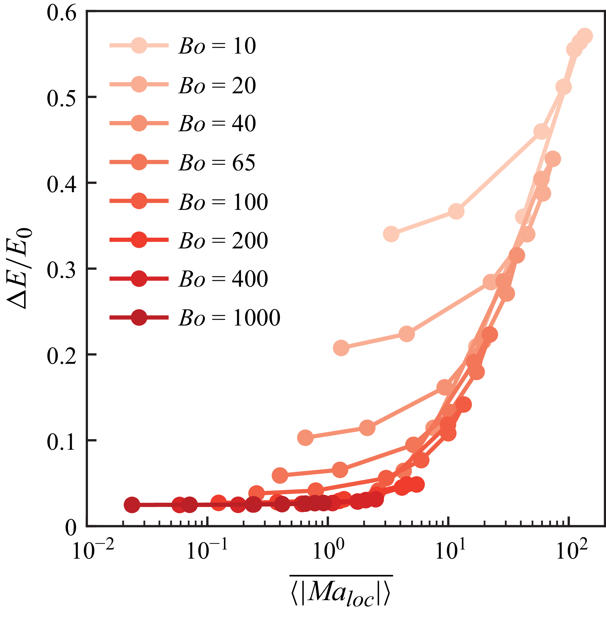


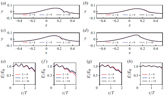


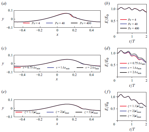


 Open access