2. Numerical model

In this work, we use a semi-implicit electromagnetic 3D3V PIC model with exact conservation of global energy and local charge (Berendeev et al. Reference Berendeev, Timofeev and Kurshakov2024). The model may not resolve the electron plasma frequency $\omega _{pe}=\sqrt {4\pi e^2 n_0/m_e}$ and the Debye radius, but it requires resolution of the cyclotron rotation of electrons, $\Delta t\lt \varOmega _e^{-1}$ (here $e$ is the absolute value of charge for ions and electrons, $m_e$ is the mass of an electron, $n_0$ is the characteristic plasma density, $\varOmega _e=eB/(m_ec)$ is the cyclotron frequency of electrons in a magnetic field $B$ and $\Delta t$ is the time step). Thus, the temporal step is chosen equal to $\Delta t=1.5\,\omega _{pe}^{-1}\approx 0.3 \varOmega _e^{-1}$ . 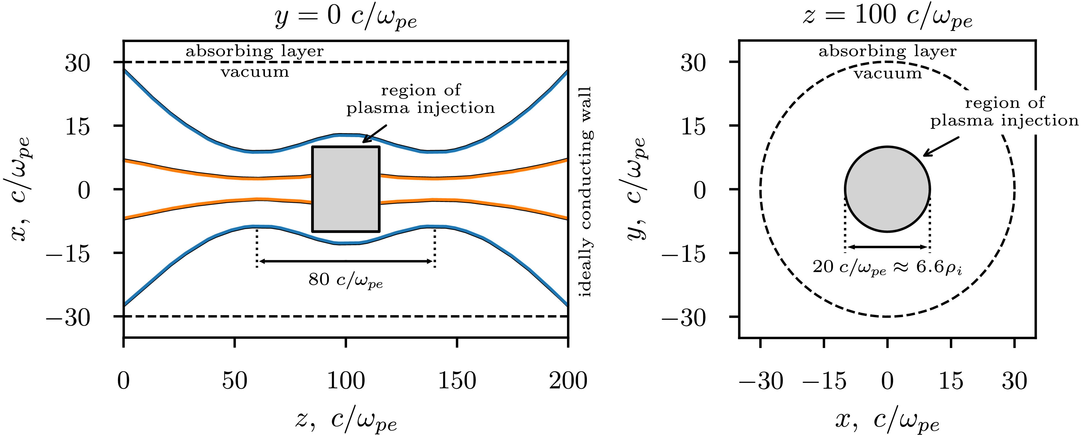The grid step must resolve the transition layer that can be less than the ion gyroradius, and the use of the value $\Delta x=0.5\,c/\omega _{pe}$ is justified for this purpose by our recent quasi-two-dimensional simulations (Timofeev et al. Reference Timofeev, Kurshakov and Berendeev2024). In order to qualitatively reproduce the process of continuous growth of plasma pressure, which in the CAT experiment is provided by constant injection of high-energy hydrogen atoms with energy of 15 keV, we use a simplified injection model, in which electron–ion pairs with Maxwellian velocity distribution are uniformly thrown into a selected cylindrical region with radius 10 $c/\omega _{pe}$ and length 30 $c/\omega _{pe}$ ( $c$ is the speed of light), located in the centre of the mirror trap (figure 1). The temperatures of injected particles are chosen lower ( $T_e=T_i=1$ keV) for reasons of saving computing time. The injection-induced growth rate of plasma density ( ${\rm d}n/{\rm d}t=n_0/\tau$ ) is determined by the characteristic time $\tau$ , which is much shorter than the experimental time scale, but large enough to ensure that a quasi-stationary equilibrium is established at each moment of time. This is achieved if the injection time exceeds the period of ion Larmor rotation $\tau =5000\,\omega _{pe}^{-1}\approx 1.5(2\pi /\varOmega _i)$ . Coulomb collisions are not taken into account. By the end of the simulations, the number of macroparticles per cell in the plasma centre reaches 3000, and their full number exceeds $10^9$ . To reduce the simulation time, we use a reduced ion mass $m_i/m_e=100$ and a smaller distance between the plugs $L=80\,c/\omega _{pe}$ (at $n_0=10^{13}$ cm $^{-3}$ it is 13.6 cm), but we maintain the same relationship between the flute instability growth rate and the ion-cyclotron frequency ( $\varGamma /\varOmega _i\sim 1$ ), which should be realised in the experiment. The regime of such rapid development of instability, when plasma ions cease to be frozen into the magnetic field lines, is the main subject of our research.

Figure 1. The layout of the simulation box.

The vacuum magnetic field ${\boldsymbol{B}}_v({\boldsymbol{r}})$ in our simulations is calculated as a field from two infinitely thin current coils and is characterised by the same mirror ratio $R=2$ that is created in the compact mirror cell of the CAT facility. The simulation starts from a state when there are no particles in the computational domain, therefore ${\boldsymbol{E}}(0,{\boldsymbol{r}})=0$ , and ${\boldsymbol{B}}(0,{\boldsymbol{r}})={\boldsymbol{B}}_v({\boldsymbol{r}})$ . As for the boundary conditions, along the trap axis at $z=0$ and $z=200\,c/\omega _{pe}$ we always place perfectly conducting walls on which the tangential components of the electric field and the normal component of the magnetic field vanish ( $\textit {E}_{x,y}(t,x,y)=\textit {B}_z(t,x,y)=0$ ), and in the transverse directions we consider three different options. In the first case, on the lateral cylindrical surface with a radius of 30 $c/\omega _{pe}$ we place an absorbing layer (as shown in the figure 1), inside which all disturbances of electromagnetic fields are multiplied by a decreasing coefficient and gradually attenuate with distance from the boundary. The second option assumes that the same cylindrical surface is perfectly conductive. In this case, all electric fields and magnetic field perturbations are precisely zero at all Cartesian grid nodes whose distance from the system axis exceeds a given radius. In the third case, the conductive boundaries coincide with the square lateral boundaries of the computational domain.

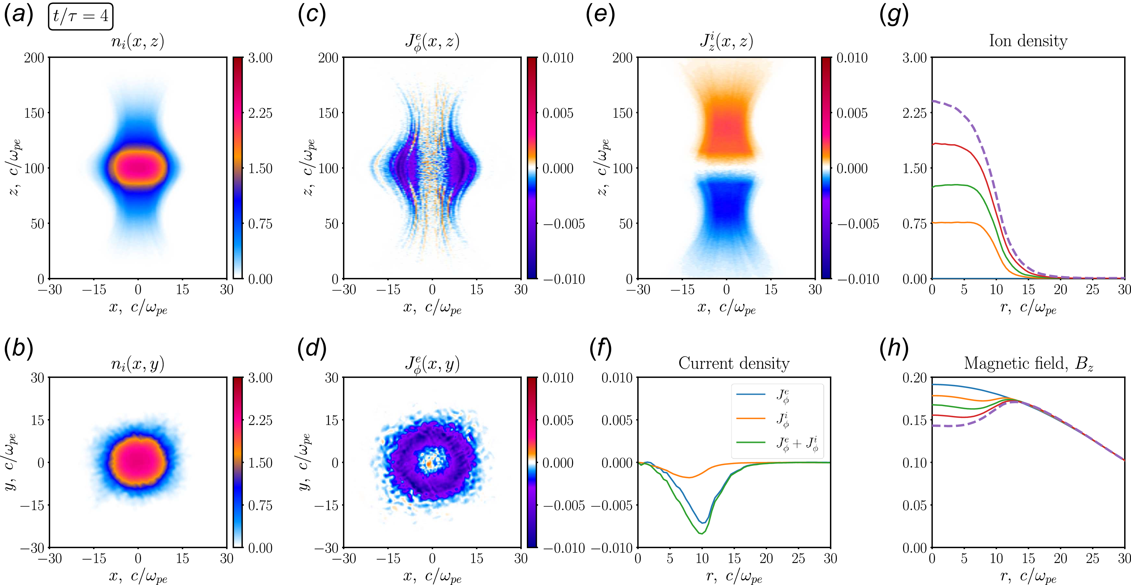
Figure 2. Initial stage of injection: (a) map of the ion density $n_i(x,z)$ in the longitudinal section of the plasmoid ( $y=0$ ) at time $t=4\tau$ ; (b) map of the ion density $n_i(x,y)$ in the central cross-section of the plasmoid ( $z=100\,c/\omega _{pe}$ ) at time $t=4\tau$ ; (c) map of the electron azimuthal current density $J_{\phi }^e(x,z)$ at $y=0$ at time $t=4\tau$ ; (d) map of the electron azimuthal current density $J_{\phi }^e(x,y)$ at $z=100\,c/\omega _{pe}$ at time $t=4\tau$ ; (e) map of the longitudinal ion current density $J_{z}^i(x,z)$ at $y=0$ and time $t=4\tau$ ; (f) $\phi$ -averaged radial profiles of the electron $J_{\phi }^e(r)$ , ion $J_{\phi }^i(r)$ and total current $J_{\phi }^e+J_{\phi }^i$ at $z=100\,c/\omega _{pe}$ ; (g) $\phi$ -averaged radial profiles of the ion density $n_i(r)$ at $z=100\,c/\omega _{pe}$ at times $t=0,\tau ,2\tau ,3\tau ,4\tau$ ; (h) averaged over $\phi$ radial profiles of the magnetic field $B_z(r)$ at $z=100\,c/\omega _{pe}$ at times $t=0,\tau ,2\tau ,3\tau ,4\tau$ .

3. Quasi-stationary equilibrium

Let us initially consider the first case, which corresponds to the absence of a sidewall. At the initial stage of injection $t\lt 4\tau$ the plasma remains axially symmetric, which can be seen from the spatial distributions of the ion density and electron current density shown in figure 2(a–d) in the $(x,z)$ and $(x,y)$ planes. These planes represent the longitudinal ( $y=0$ ) and transverse ( $z=100\,c/\omega _{pe}$ ) cross-sections of the formed plasma. Small-scale ripples at the plasma periphery are the result of the development of drift ion-cyclotron instability, which we studied in detail in two-dimensional simulations with a uniform vacuum magnetic field (Kurshakov & Timofeev Reference Kurshakov and Timofeev2023; Timofeev et al. Reference Timofeev, Kurshakov and Berendeev2024). Averaging over the azimuthal angle in the central cross-section, we obtain radial profiles of various quantities shown in figure 2(f–h). It can be seen that at this stage, the continuous injection of particles leads to a constant increase in plasma density (figure 2 g). Since the pressure also increases with density, this process is accompanied by the displacement of the magnetic field from the volume occupied by the plasma (figure 2 h). It is interesting to note that the three-dimensional simulations with conducting ends presented here demonstrate the formation of the same type of equilibrium that was observed in the quasi-two-dimensional simulations (Timofeev et al. Reference Timofeev, Kurshakov and Berendeev2024) with periodic boundary conditions assuming an infinite length of the plasma column. The main feature of this equilibrium is that the azimuthal current is created almost entirely by electrons. The comparison of the radial profiles of electron and ion azimuthal current densities shown in figure 2(f) confirms the complete dominance of electrons. Figure 2(e) shows the spatial distribution of the longitudinal current of ions accelerated by the ambipolar potential and confirms the presence of plasma contact with the end walls. This current, of course, is completely compensated by the electron current $J_z^e$ .

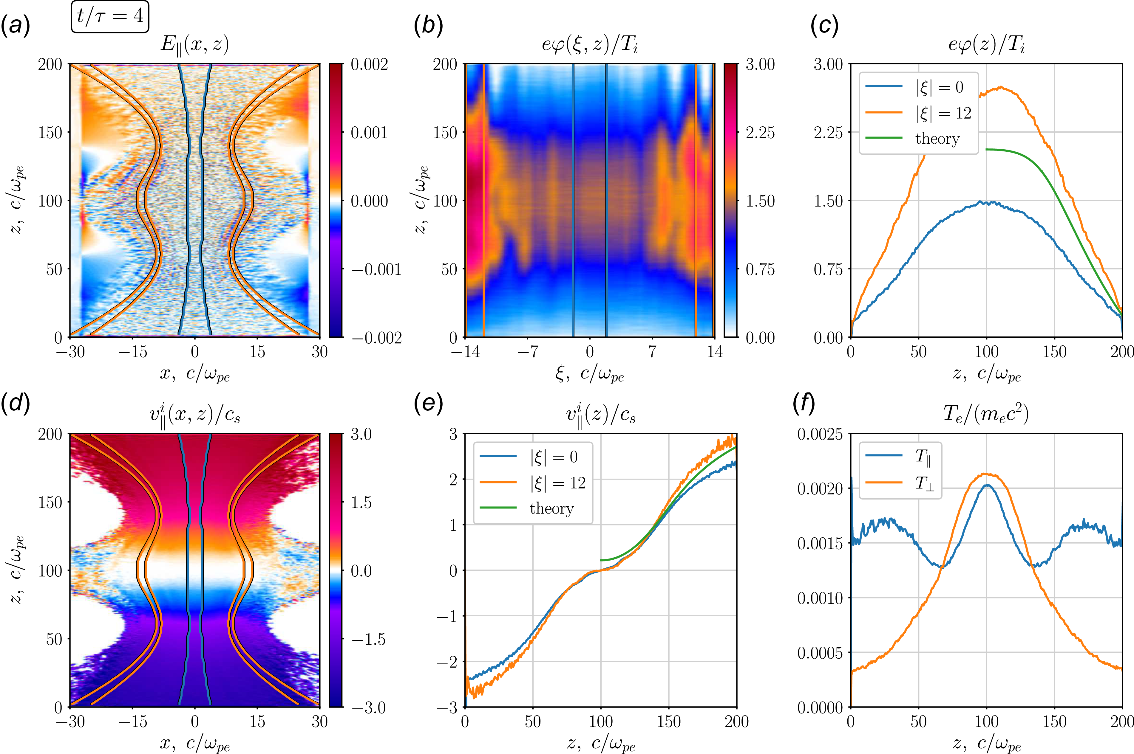
Figure 3. (a) Map of the longitudinal electric field $E_{\|}(x,z)$ (blue and orange lines distinguish two magnetic flux tubes); (b) map of the electric potential $\varphi (\xi ,z)$ , where $\xi$ is the $x$ coordinate of the field line at $z=100\,c/\omega _{pe}$ ; (c) longitudinal profiles of the potential $\varphi (z)$ averaged over the central (blue) and peripheral (orange) field tubes; (d) map of the longitudinal ion velocity $v_{\|}^i(x,z)$ in units of the speed of sound $c_s$ ; (e) longitudinal profiles of the ion velocity $v_{\|}^i(z)/c_s$ , averaged over the central (blue) and peripheral (orange) flux tubes (green lines are the theoretical predictions from Smolyakov et al. (Reference Smolyakov, Sabo, Yushmanov and Putvinskii2021)); (f) axial profiles of the transverse and longitudinal electron temperatures $T_{\|}/m_ec^2=2\varPi _{zz}^e/n_e$ and $T_{\bot }/m_ec^2=\varPi _{rr}^e/n_e$ .

At equal temperatures, ions and electrons should create equal diamagnetic currents. The reason for the dominance of the electron azimuthal current is the formation of a transverse jump in electric potential at the centre of the trap. This jump is produced by ions having greater Larmor orbits and creating an excess positive charge on the plasma periphery. In real traps this positive charge can be completely or partly compensated by cold secondary electrons emitted from plasma receivers. In our simulations, secondary emission is not yet realised, so the observed potential jump in the transverse direction is apparently greater than in reality. Further we specify the main peculiarities of the observed equilibrium. Figure 3(a) shows a map of the longitudinal electric field $E_{\|}(x,z)=({\boldsymbol{E}}\boldsymbol{\cdot }{\boldsymbol{B}})/B$ . To obtain the potential $\varphi (\xi ,z)$ , we must integrate $E_{\|}$ along the magnetic field lines, each of which we will characterise by the transverse coordinate $\xi =x(z=100)$ in the central cross-section of the plasma. The result of this integration is shown in figure 3(b). Let us now select two flux tubes, one of which encircles the axis of the system (solid blue lines in figure 3 a), and the second one passes along the periphery of the plasma (solid orange lines in figure 3 a). In figure 3(b), these tubes become straight. Averaging over them, we obtain the longitudinal profiles of the electric potential $\varphi (z)$ shown in figure 3(c). The blue curve here corresponds to the central flux tube, and the orange one to the peripheral flux tube. It is evident that the radial potential jump in the central cross-section of the plasma $\Delta _{\bot }\varphi \approx 1.5\,T_e/e$ has the same magnitude as the longitudinal drop in the ambipolar potential $\Delta _{\|}\varphi \approx 1.5\,T_e/e$ between the wall and the centre of the plasma on the trap axis. Since this radial jump is comparable to the ion temperature $\Delta _{\bot }\varphi \sim T_i/e$ , one should expect that the ion confinement in the transverse direction should be largely electrostatic. Figure 3(d,e) shows maps of the longitudinal ion velocity $v_{\|}^i=({\boldsymbol{v}}_i\boldsymbol{\cdot }{\boldsymbol{B}})/B$ in the $(x,z)$ plane and the axial profiles $v_{\|}^i(z)$ averaged over the same flux tubes in units of the speed of sound $c_s=\sqrt {T_e/m_i}$ . It can be seen that when moving from the central tube to the peripheral one, the speed of ions accelerated by the ambipolar potential increases from 2.4 $c_s$ to 2.9 $c_s$ . It is also interesting to demonstrate how the obtained results agree with the simplified theoretical model of plasma acceleration by a magnetic nozzle, constructed in Smolyakov et al. (Reference Smolyakov, Sabo, Yushmanov and Putvinskii2021) for cold ions and an isothermal Boltzmann electron distribution. In figures 3(c) and 3(e), the predictions of this theory for the central field line ( $r=0$ ) are shown by the green curves. In agreement with this theory, the ion flow velocity in our simulations reaches the speed of sound precisely in magnetic plugs. In contrast to the theoretical assumption, the electron temperature significantly decreases in expanders and becomes not only non-uniform, but also anisotropic in our simulations (figure 3 f), so that the observed axial drop in potential (blue curve) turns out to be smaller than in theory. The lower potential drop results in the lower flow velocity of ions.

Figure 4. (a) Balance of longitudinal forces from the equilibrium equation (3.1); (b) transverse equilibrium for ions (different curves show the relative contribution of different terms in (3.7)); (c) similar transverse equilibrium for electrons (all panels are drawn for time $t=4\tau$ ).

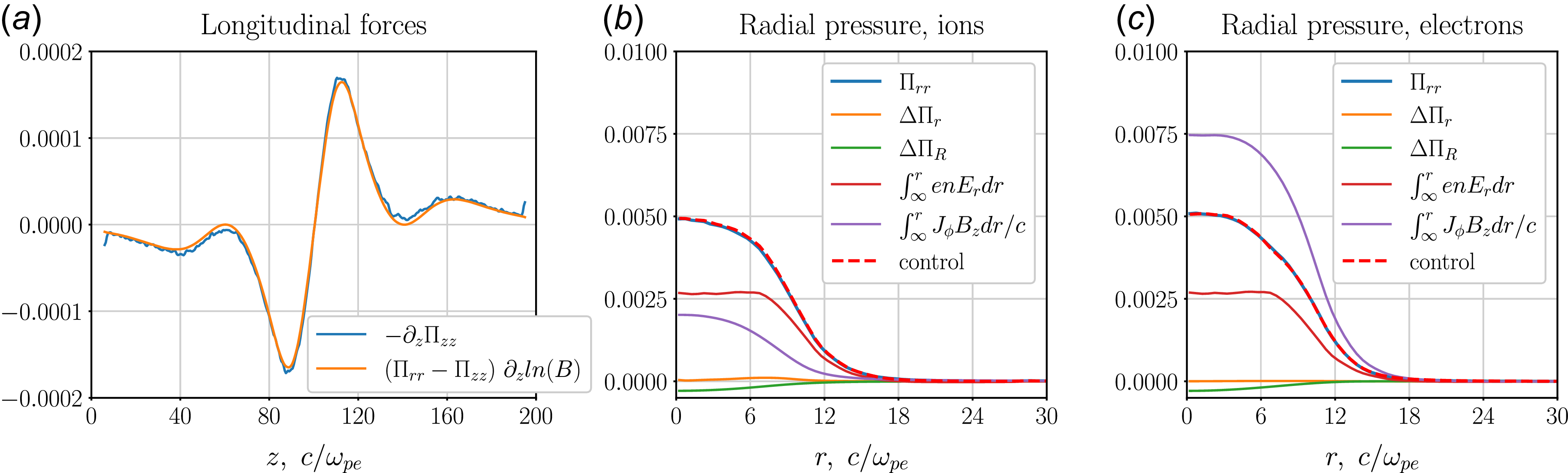
To confirm the important role played by the radial electric field in the formation of the observed equilibrium, we compare the relative contributions of the different forces to the overall balance. Before this, let us make sure that the plasma is in longitudinal equilibrium. After summing the contributions of electrons and ions, the balance of longitudinal forces at $r=0$ can be written as

(3.1) \begin{equation} -\frac {\partial \varPi _{zz}}{\partial z}+\frac {\varPi _{zz}-\varPi _{rr}}{B_z} \frac {\partial B_z}{\partial z}=0, \end{equation}

where $\varPi _{\alpha \beta }$ is the tensor of the total momentum flux carried by the particles:

(3.2) \begin{align} &\varPi _{zz}=\sum \limits _{s=i,e}\varPi _{zz}^s, \quad \varPi _{zz}^s=\int m_s v_z^2 f_s \,\text{d}\textbf {v}, \end{align}

(3.3) \begin{align} &\varPi _{rr}=\sum \limits _{s=i,e}\varPi _{rr}^s, \quad \varPi _{rr}^s=\int m_s v_r^2 f_s \,\text{d}\textbf {v}. \end{align}

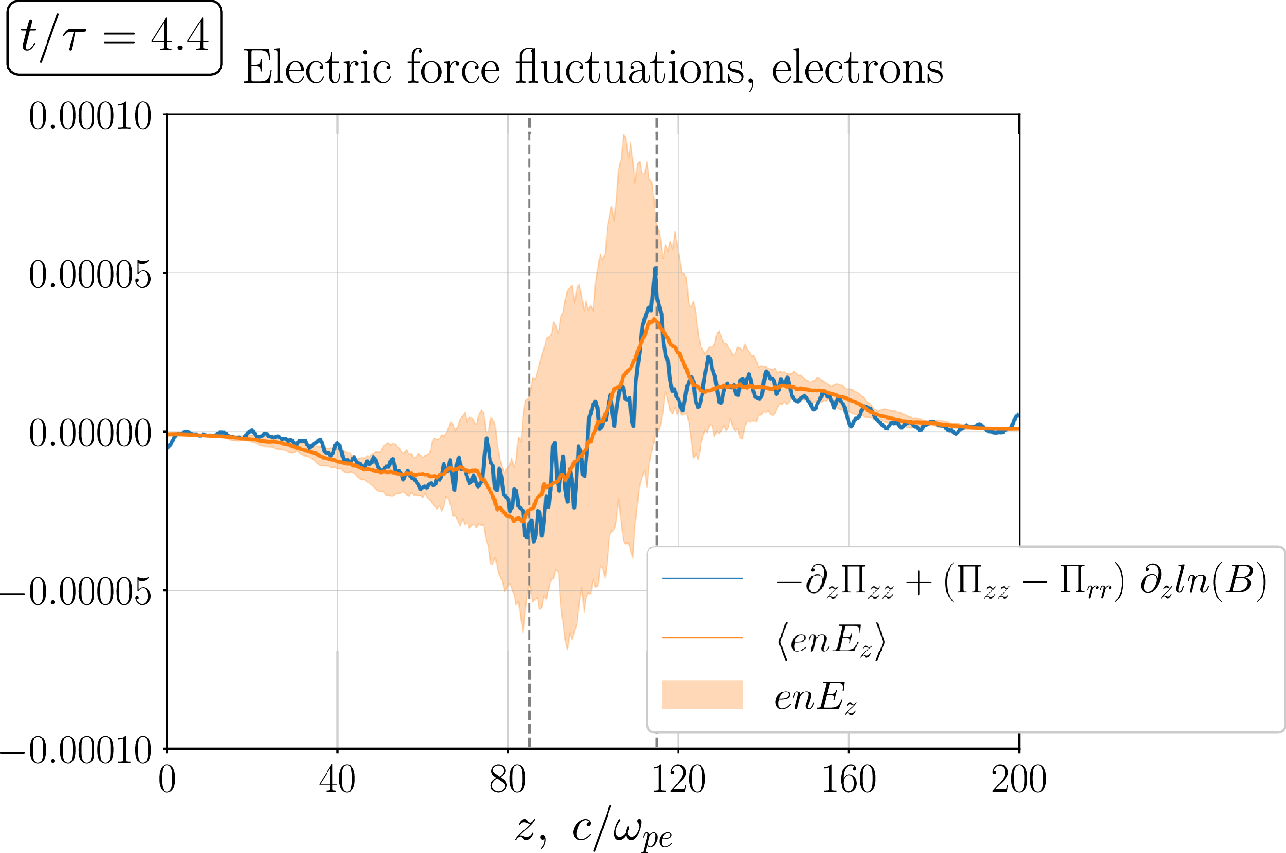
Figure 5. Longitudinal force balance for electrons. The blue curve shows the $z$ dependence of forces from the left-hand side of (3.4), and the orange curve corresponds to the electric force from the right-hand side of (3.4) averaged over 20 time steps. The orange stripe is a region swept out by instantaneous profiles of electric force in these 20 moments of time.

From figure 4(a), it is clear that the two terms in (3.1) do indeed cancel each other out. But if we consider the same balance separately for electrons,

(3.4) \begin{equation} -\frac {\partial \varPi _{zz}^e}{\partial z}+\frac {\varPi _{zz}^e-\varPi _{rr}^e}{B_z} \frac {\partial B_z}{\partial z}=en_eE_z, \end{equation}

we find that it is satisfied only on average (figure 5) because of a strongly fluctuating electric field. Figure 5 shows how instantaneous field profiles, measured during 20 time steps and sweeping the orange area, can deviate from that averaged over the same interval. These fluctuations are localised inside the injection region and are apparently excited by the injected particles, since fast Langmuir oscillations as proper plasma modes are still resolved in our model ( $2\pi /\omega _{pe}\approx 4.2\Delta t$ ). Strong instantaneous violation of the force balance means that electron inertia cannot be neglected, and electrons must not be frozen into magnetic field lines.

As for radial equilibrium in the central cross-section ( $z=100\,c/\omega _{pe}$ ), we also examine it separately for each type of particle using the same time averaging:

(3.5) \begin{equation} -\frac {\partial \varPi _{rr}^{e,i}}{\partial r}-\frac {\varPi _{rr}^{e,i}-\varPi _{\varphi \varphi }^{e,i}}{r}-\frac {\varPi _{rr}^{e,i}-\varPi _{zz}^{e,i}}{\mathcal{R}} \mp en_{e,i} E_r+\frac {J_{\varphi }^{e,i} B_z}{c}=0. \end{equation}

Here, in addition to the non-gyrotropic effect ( $\varPi _{rr}\neq \varPi _{\phi \phi }$ ), which begins to play an important role at large $\beta$ (Kotelnikov Reference Kotelnikov2020; Timofeev et al. Reference Timofeev, Kurshakov and Berendeev2024), we also take into account the curvature of the magnetic field lines. We calculate the radius of this curvature $\mathcal{R}$ in the paraxial approximation using the known dependence of the magnetic field modulus on the axis $B=B_z(0,z)$ :

(3.6) \begin{equation} \frac {1}{\mathcal{R}}=-\frac {\text{d}^2 r}{\text{d}z^2}=\frac {r}{2B}\left (B^{\prime \prime }-\frac {3 (B^{\prime })^2}{2B}\right )\!. \end{equation}

To show the contributions of individual terms more clearly, we integrate (3.5) over the radius and represent it as a pressure balance:

(3.7) \begin{align} \varPi _{rr}^{e,i}(r)&=\int \limits _{\infty }^r \frac {J_{\varphi }^{e,i}B_z}{c}\,\text{d}r^{\prime }\mp \int \limits _{\infty }^r en_{e,i}E_r\,\text{d}r^{\prime } \nonumber \\ &\quad-\int \limits _{\infty }^r \frac {\varPi _{rr}^{e,i}-\varPi _{\varphi \varphi }^{e,i}}{r^{\prime }}\,\text{d}r^{\prime }-\int \limits _{\infty }^r \frac {\varPi _{rr}^{e,i}-\varPi _{zz}^{e,i}}{\mathcal{R}}\,\text{d}r^{\prime }. \end{align}

From figures 4(b) and 4(c) it is evident that the contribution of the radial electric force (red solid line) is approximately half of the pressures $\varPi _{rr}$ created by ions and electrons (blue lines). The appearance of this force decreases the Lorentz force for ions and increases the Lorentz force for electrons by the same amount. In other words, the ${\boldsymbol{E}}\times {\boldsymbol{B}}$ drift arising from the radial electric field slows down the azimuthal motion of ions and accelerates the azimuthal motion of electrons, leading to the observed dominance of the electron current. At the stage under consideration ( $t=4\tau$ ), the non-gyrotropic effect $\Delta \varPi _r$ , described by the third term on the right-hand side of (3.7), turns out to be negligibly small (orange curves in the figure), which cannot be said about the effect of finite curvature $\Delta \varPi _R$ (the last term on the right-hand side of (3.7)). Without the curvature term, the observed agreement between the left (blue lines) and right (red dashed lines) parts of the equation could not have been achieved. Thus, despite the high plasma injection rate, after averaging over fast space-charge oscillations, the spatial distributions of fields and particles observed in the simulations satisfy the stationary equilibrium equations at each moment of time. This agreement is violated at the stage of the flute instability development.

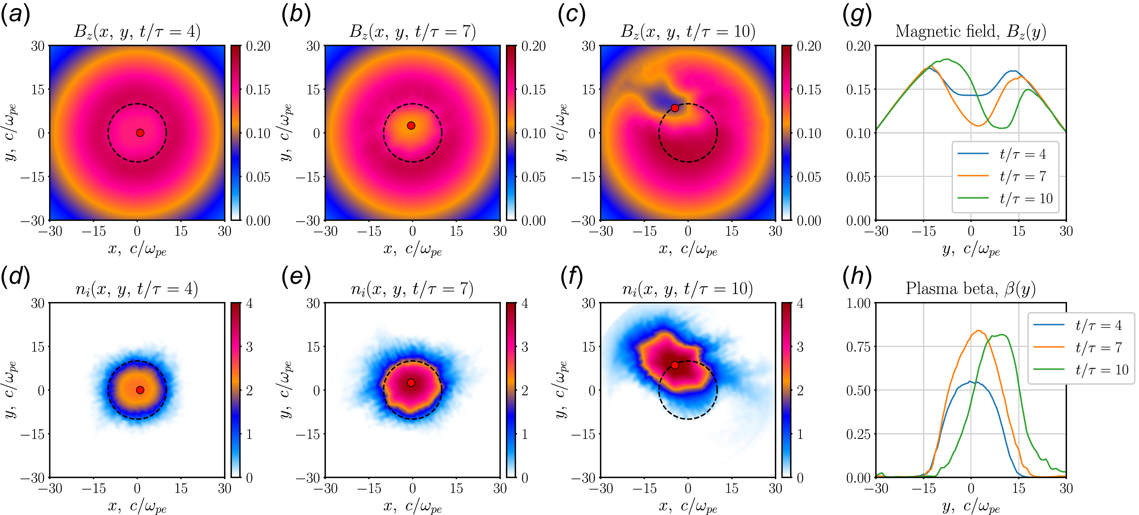
Figure 6. Development of the flute instability: (a–c) maps of the magnetic field $B_z(x,y)$ in the central cross-section at different times; (d–f) maps of the ion density $n_i(x,y)$ at the same times; (g) transverse profiles of the magnetic field $B_z(0,y)$ at the same times; (h) transverse profiles of the relative plasma pressure $\beta (y)=2\varPi _{rr}(0,y)/B_v^2$ .

4. Flute-like instability

As the relative pressure increases (at $\beta \gt 0.5$ ), the plasma becomes unstable with respect to flute perturbations that disrupt the axial symmetry of the plasma column. According to the criterion of Ryutov et al. (Reference Ryutov, Berk, Cohen, Molvik and Simonen2011), the effects of a finite Larmor radius should lead to the stabilisation of all flute perturbations whose azimuthal numbers exceed the value

(4.1) \begin{equation} m\gt 2\frac {a/\rho _i}{L/a}\approx 1. \end{equation}

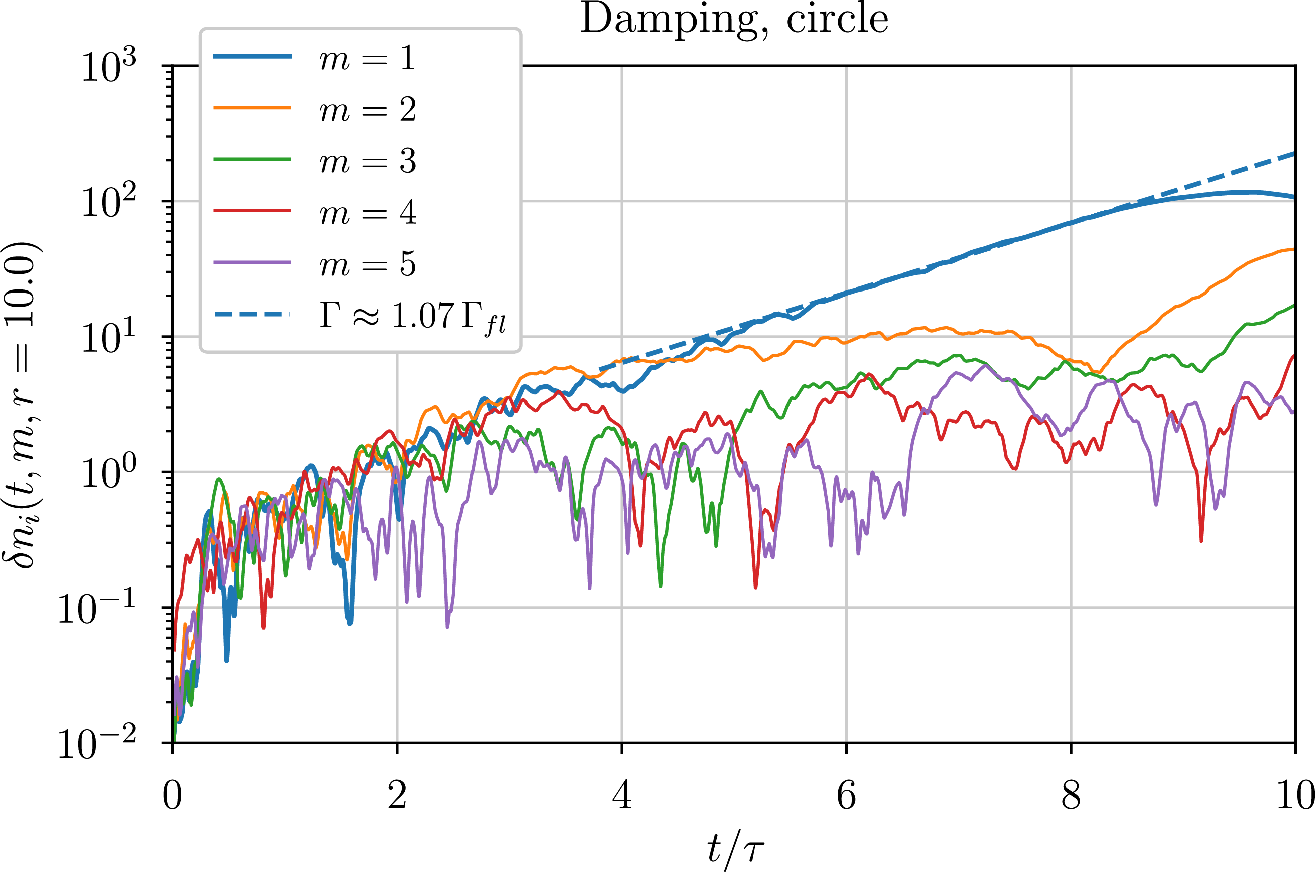
In figure 7, we show the growth of the first five azimuthal harmonics of ion density perturbations measured at a fixed radius $r=10\,c/\omega _{pe}$ . It is evident that, unlike higher modes, the stage of long-term exponential growth is observed only for the $m=1$ mode. Its development leads to the displacement of the plasma bunch from its original position, followed by the ejection of plasma onto the wall. The dynamics of this process on the maps of plasma density $n_i(x,y)$ and longitudinal magnetic field $B_z(x,y)$ in the central cross-section of the plasma is shown in figure 6. It is also seen from the figure 6(h) that due to the development of this instability, the parameter $\beta$ does not reach its magnetohydrodynamic limit $\beta =1$ . 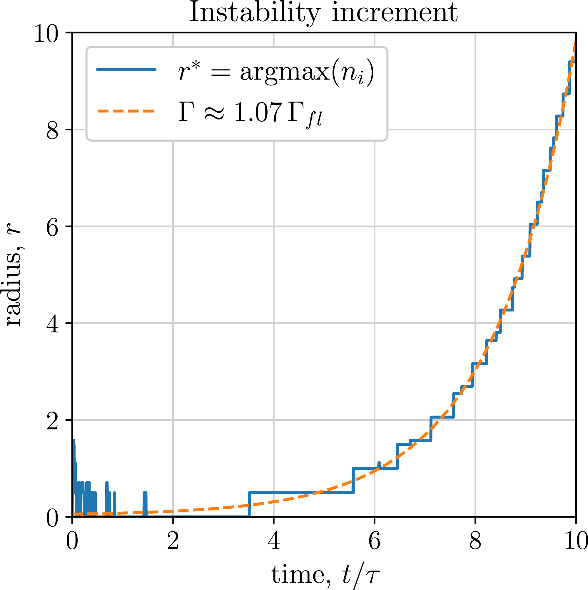The growth rate of the $m=1$ mode can be determined either from the exponential stage of the harmonic amplitude growth measured at a fixed radius or from the dynamics of the radial displacement of the point at which the maximum value of the plasma density is reached. Figure 8 shows that the shift of the point of maximum density does really grow exponentially, and the rate of this growth is in good agreement with the known estimate of the inverse time that is needed for ions to move half the distance between the mirrors $\varGamma _{fl}=v_{Ti}/(L/2)$ , where $v_{Ti}=\sqrt {T_i/m_i}$ is the thermal velocity of the ions.

Figure 7. Amplitudes of the harmonics of ion density perturbations at a radius of $r=10\, c/\omega _{pe}$ with different azimuthal numbers $m$ as functions of time (the blue dashed line corresponds to the exponential function with an increment of $\varGamma =1.07\, \varGamma _{fl}$ ).

Figure 8. The dependence of the radial shift of the maximal ion density on time, measured in simulations (blue curve), and the exponential function ${\rm e}^{\varGamma t}$ inscribed in this curve (orange curve).

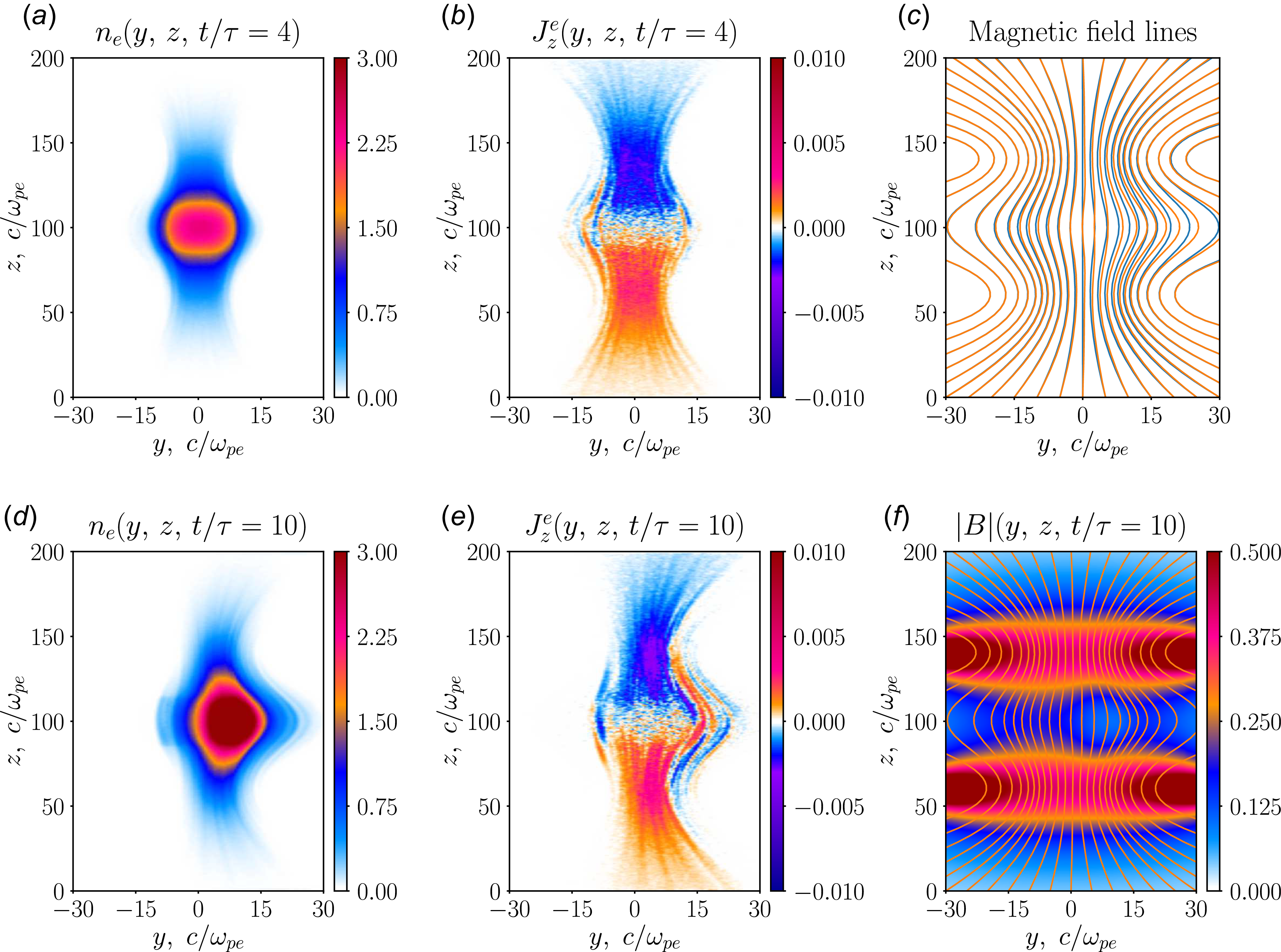
Based on the nature of the plasma displacement in the $(y,z)$ plane, shown on the $n_e(y,z)$ and $J_\phi ^e(y,z)$ maps in figure 9, one can conclude that there is no plasma freezing into the magnetic field lines. Indeed, despite the line-tying to the end walls, the movement of plasma from the axis to the periphery occurs along the entire length of the trap. In our opinion, this behaviour is explained by the fact that ions are not tied to magnetic field lines, since they do not have time to complete Larmor rotation during the development of such a fast instability, and electrons cease to be frozen into the magnetic field due to high level of electrostatic fluctuations excited inside the injection region. So the plasma can quickly diffuse in the central part of the trap across the magnetic field, then flowing out to the ends along the peripheral field lines. This picture is confirmed by figure 9 showing the tension of magnetic field lines that accompanies the displacement of the plasma bunch during the instability. In figure 9(c), we superimpose the orange magnetic field lines constructed from $B$ distribution (figure 9 f) at the stage of developed flute instability ( $t/\tau =10$ ) on the blue magnetic field lines realised in the stable plasma ( $t/\tau =4$ ). It can be seen that these field lines are slightly deformed and stretched in the direction of plasma movement, but their displacement is much less than the displacement of the centre of the plasma bunch shown in figure 8.

Figure 9. Simulation results for the absorbing sidewall. (a,b) Spatial distributions of the electron density $n_e(y,z)$ and the density of their longitudinal current $J_z^e(y,z)$ in the longitudinal cross-section of the plasma at the moment of time $t=4\tau$ when the plasma still remains axially symmetric, and (d,e) after the growth of the flute mode $m=1$ at the time $t=10\tau$ ; (c) superposition of magnetic field lines in the longitudinal $(y,z)$ cross-section of plasma measured before ( $t=4\tau$ , blue) and after ( $t=10\tau$ , orange) the development of instability; (f) magnetic field lines at $t=10\tau$ superimposed on the map $|B(y,z)|$ at the same cross-section.

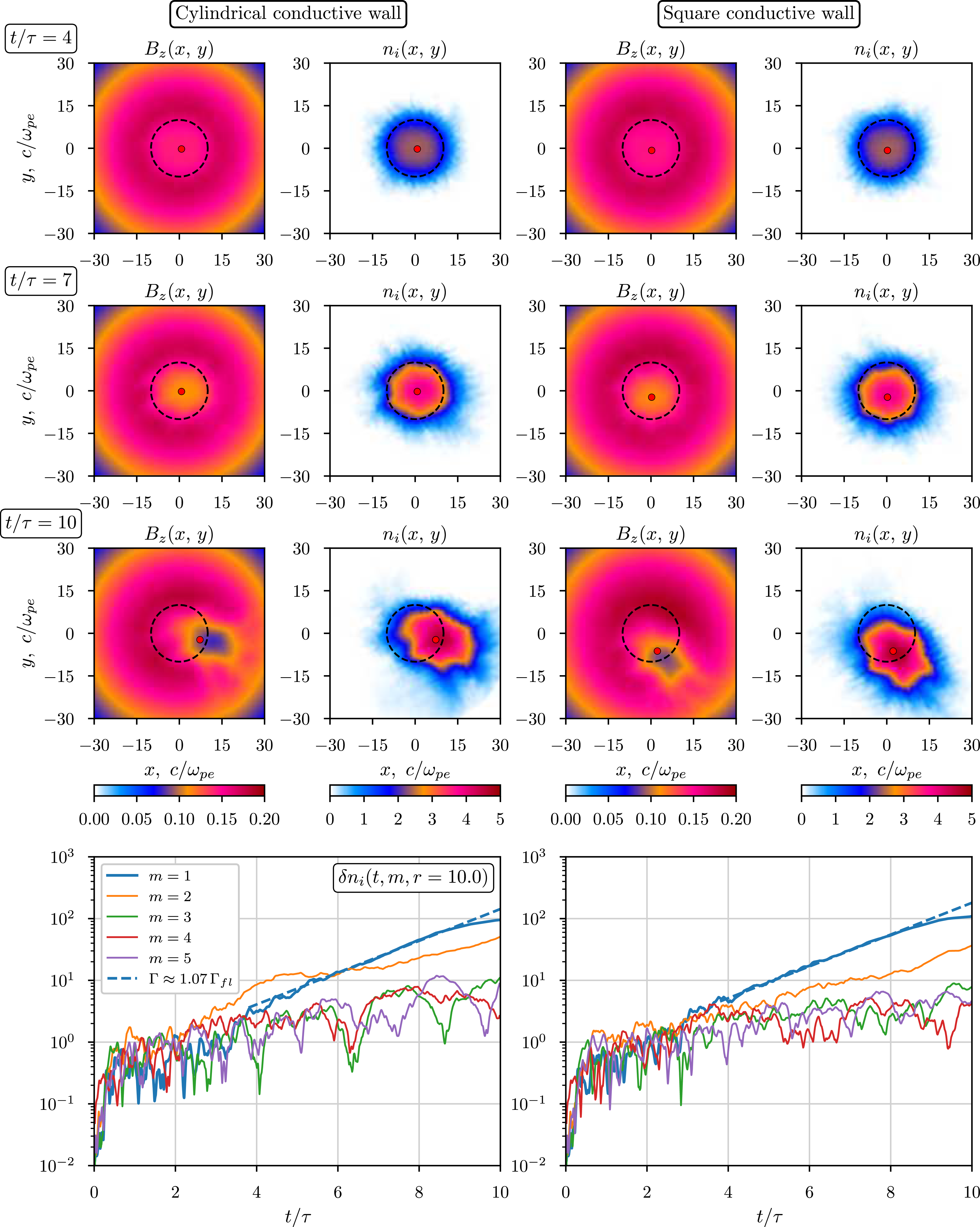
Figure 10. Development of the flute instability in the presence of conducting cylindrical (left) and square (right) sidewalls (maps of the longitudinal magnetic field $B_z(x,y)$ and ion density $n_i(x,y)$ at three instants are shown). The dashed line shows the boundaries of the injection region. Growth of various azimuthal harmonics of plasma density perturbations at a radius of 10 $c/\omega _{pe}$ with time for different wall shapes (bottom panels).

5. Effect of conducting wall

Let us now explore the possibility of stabilising this instability using perfectly conducting sidewalls. We consider both cylindrical and square sidewalls. The radius of the circular wall is 30 $c/\omega _{pe}$ , and the square wall coincides with the boundaries of the computational domain with dimensions 70 $c/\omega _{pe}\times$ 70 $c/\omega _{pe}$ . Maps of the longitudinal magnetic field and ion density (figure 10), shown at the same moments of time as in the case of the absorbing sidewall, demonstrate similar dynamics of the development of the flute instability. An analysis of the amplitudes of the density perturbation harmonics with different azimuthal numbers at a radius of 10 $c/\omega _{pe}$ (bottom row in figure 10) shows that in the case of a cylindrical conducting wall, the most unstable mode is initially the $m=2$ mode. Then its growth quickly stabilises, so that, as before, the dominant role in the unstable spectrum passes to the $m=1$ mode. The square shape of the wall, contrary to intuitive expectations, does not create additional preferences for the development of higher modes ( $m=4$ ), and the displacement of the column as a whole from the equilibrium position increases exponentially with the same growth rate.

We attribute the absence of a stabilising effect from the conducting walls in the presented simulations to the fact that the growth rate of flute instability turns out to be comparable to the ion-cyclotron frequency ( $\varGamma \sim \varOmega _i$ ), due to which the ions, with such rapid transverse displacements, cease to be tied to the magnetic field lines. Electrons also cannot be considered frozen in the magnetic field in our simulations due to rapid electrostatic oscillations at the plasma frequency excited in the injection region. This means that the displacement of the plasma under these conditions occurs without noticeable tension of the magnetic field lines frozen into the ends and without the generation of a sufficiently strong longitudinal current, which should increase the magnetic pressure as the plasma gradually approaches the wall due to generating an azimuthal component of the field $B_\phi$ .

6. Summary

The formation of a compact high-beta plasma in the central part of an open magnetic trap is modelled for the first time in three-dimensional geometry using a full kinetic description of both ions and electrons. It is shown that in the process of continuous injection of particles into the centre of the trap, a quasi-stationary equilibrium is formed, in which the radial electric field leads to the dominance of the electron azimuthal current. The numerical model is found to correctly reproduce the development of flute instability with azimuthal number $m=1$ and demonstrates stabilisation of higher azimuthal modes at relatively low saturation levels. Simulations revealed no stabilising effect on this instability from either the end or side conductive walls. We attribute this to (i) the very small longitudinal size of the formed plasma, which makes the flute instability growth rate comparable to the ion-cyclotron frequency, and to (ii) the high level of space-charge oscillations excited inside the injection region. Under these conditions, both ions and electrons are no longer frozen into the field lines, and the transverse displacement of the plasma is not accompanied by a large perturbation of the magnetic field. Although we cannot yet directly extrapolate our results to the CAT experiment due to a disregarding of the injected currents, we note that a similar relationship between $\varGamma _{fl}$ and $\varOmega _i$ can be achieved at the CAT facility, where, upon accumulation of hot ions with a characteristic energy of 10 keV, the flute instability in a mirror cell with a length of 60 cm should develop in a time of $\approx 2\times 10^{-7}$ s, not exceeding the period of the Larmor rotation of ions $2\pi /\varOmega _i\approx 3.6\times 10^{-7}$ s in a central magnetic field of 2 kG.

Further steps towards achieving a stable plasma equilibrium with $\beta =1$ will include implementation of another stabilisation technique (edge biasing) in the numerical model and a more detailed study of electrostatic noise affecting electron diffusion. It should be studied whether this noise can be reduced by (i) reducing the rate of particle injection, by (ii) increasing the gap between $\omega _{pe}$ and $\varOmega _e$ , when Langmuir oscillations cannot be resolved as proper plasma modes, or by (iii) using the realistic model of neutral beam injection. The regime of slower development of the flute instability with frozen ions will also be of interest after the increase in performance of the code.