2. Governing equations and simulation set-up

Here, we consider the flow of viscoelastic fluid past a flexibly mounted square prism with one degree-of-freedom in the cross-flow direction (figure 1). The fluid field is simulated by solving the unsteady, incompressible Navier–Stokes (N-S) equations,

(2.1) \begin{align} \boldsymbol{\nabla }\boldsymbol{\cdot }\boldsymbol{u}=0, \\[-28pt] \nonumber \end{align}

(2.2) \begin{align} \rho \left (\dfrac {\partial \boldsymbol u}{\partial t}+\boldsymbol{u}\boldsymbol{\cdot }\boldsymbol{\nabla } \boldsymbol{u}\right )=-\boldsymbol{\nabla }\!p+\boldsymbol{\nabla }\boldsymbol{\cdot }\boldsymbol{\tau }. \\[0pt] \nonumber \end{align}

The total stress tensor, $\boldsymbol \tau =\boldsymbol \tau _{\!s}+\boldsymbol \tau _{\!p}$ , consists of a solvent contribution, $\boldsymbol{\tau} _{\!s}$ , and a polymer contribution, $\boldsymbol{\tau} _{\!p}$ , and accounts for both viscous stress and elastic stress. The solvent contribution, $\boldsymbol{\tau} _{\!s}$ , is modelled as Newtonian viscosity, $\boldsymbol \tau _{\!s}=\eta _{\!s} (\boldsymbol{\nabla u}+\boldsymbol{\nabla u}^T )$ . We use the FENE-P constitutive equations (Bird, Dotson & Johnson Reference Bird, Dotson and Johnson1980) to model viscoelasticity, where the polymeric stress is defined as

(2.3) \begin{gather} \boldsymbol{\tau _{\!p}}=\frac {\eta _{\!p}}{\lambda }\left (f\boldsymbol{A}-\boldsymbol{I}\right )\!, \end{gather}

in which $f=({L^2-3}/{L^2-tr(\boldsymbol{A})})$ , $\lambda$ is the relaxation time and $L$ is the maximum extensibility of the polymer. The conformation tensor, $\boldsymbol{A}$ , evolves as

(2.4) \begin{gather} {\boldsymbol{A}_{(1){}}}=-\frac {1}{\lambda }\left (f\boldsymbol{A}-\boldsymbol{I}\right )\!, \end{gather}

in which ${\boldsymbol{A}_{(1)}}=({\partial \boldsymbol{A}}/{\partial t})+\boldsymbol u\boldsymbol{\cdot }\boldsymbol{\nabla A}-\boldsymbol{A}\boldsymbol{\cdot }\boldsymbol{\nabla u}-\boldsymbol{\nabla u}^T\boldsymbol{\cdot }\boldsymbol{A}$ is the upper-convected derivative of $\boldsymbol{A}$ . Equation (2.4) is then iteratively integrated in each simulation time step, with an initial condition of $\boldsymbol{A}(t=0)=\boldsymbol{I}$ (zero deformation).

Figure 1.

(a) Schematic of the system: uniform flow past a flexibly mounted square prism, (b) the structured mesh of the fluid domain and (c) a sample of deformed mesh. The dynamic mesh is set such that it maintains the size and orthogonality of cells close to the boundary. Note that the the mesh might appear distorted due to rendering on different devices.

The structure is represented as a spring–mass system subject to external flow forces, with zero structural damping. The flow force in the cross-flow direction, $F_{\!y}$ , is calculated on the square surface. After solving the equation of motion, the cylinder displacement, $y$ , is used to update the mesh of the fluid field. To maintain the mesh quality as it deforms, we implement a diffusion-based smoother on mesh node displacement field by solving the modified Laplace’s equation. Detailed information on the numerical method is given by Patel, Rothstein & Modarres-Sadeghi (Reference Patel, Rothstein and Modarres-Sadeghi2022).

To solve the governing equations, we use the rheoFoam solver provided by the open-source toolbox RheoTool (Pimenta & Alves Reference Pimenta and Alves2017) built for OpenFOAM (Weller et al. Reference Weller, Tabor, Jasak and Fureby1998). The solver computes each time step using a modified SIMPLEC algorithm, which solves the constitutive equation along with the N-S equations. To address numerical instability arising from the high-Weissenberg-number problem (HWNP), we employ a method proposed by Fattal & Kupferman (Reference Fattal and Kupferman2004) to solve for $\log(\boldsymbol{A})$ instead of solving for either $\boldsymbol{A}$ or $\boldsymbol \tau _{\!p}$ . This logarithmic transformation approach prevents the numerical computations from diverging at large Weissenberg numbers. To solve unsteady N-S equations, the SIMPLEC (semi-implicit method for pressure linked equations-consistent) algorithm based on the projection method is employed. We calculate time derivatives using a backward scheme, and space derivatives of most fields using Gauss’s theorem with linear interpolation scheme (central differencing). However, all convective terms $\boldsymbol u\boldsymbol{\cdot }\boldsymbol{\nabla }(*)$ are discretised using the Gaussian deferred correction component-wise scheme with CUBISTA (convergent and universally bounded interpolation scheme for the treatment of advection), a high resolution scheme provided by RheoTool that has shown improved stability for viscoelastic flow simulations (Pimenta & Alves Reference Pimenta and Alves2017). Details of the numerical schemes are provided in our previous work (Patel et al. Reference Patel, Rothstein and Modarres-Sadeghi2023, Reference Patel, Rothstein and Modarres-Sadeghi2024).

Using this numerical set-up, we first perform a mesh convergence test for a case with $\textit{Wi}=2$ , $\textit{Re}=200$ , $m^*=2$ and $U^*=5$ , where a VIV response is expected, and a $U^*=30$ case, where galloping is expected. We report the values of the normalised oscillation amplitude, $A^*=A/D$ , where $A$ is the dimensional amplitude of oscillations, mean force coefficient acting in the streamwise direction, $\bar {C_x}$ , and the amplitude of the fluctuating forces acting in the cross-flow direction, $C_{\!y}$ , for this mesh convergence test as shown in table 1. The force coefficients are found as $C={2F}/{\rho U_\infty ^2 S}$ , where $S$ is the area on one side of the square prism. The results show a clear trend of convergence in all criteria. Considering accuracy and computational cost, $M_3$ is the final choice for the simulations presented in this study. The values of system parameters used in the simulations are shown in table 2.

Table 1.

Grid convergence test for $\textit{Wi}=2$ , $\textit{Re}=200$ , $m^*=2$ for a VIV case, $U^*=5$ , and a galloping case, $U^*=30$ . The normalised amplitude of oscillations, $A^*$ , mean streamwise force coefficient, $\bar {C_x}$ , and the amplitude of the fluctuating crossflow force, $C_{\!y}$ , are given for different meshes used.

Table 2.

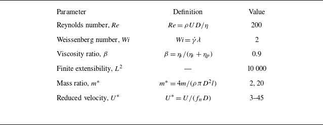
System parameters used in the simulations.

3. Observed response

We consider two mass ratios, $m^* = 2$ and 20, over a range of reduced velocities, $U^* = 3$ to 45. The viscosity ratio is set to $\beta = 0.9$ and the maximum extensibility to $L^2 = 10\,000$ . The Reynolds and Weissenberg numbers are fixed at $\textit{Re} = 200$ and $\textit{Wi} = 2$ , respectively. For both mass ratios, we first discuss the VIV response and then the galloping response for both Newtonian and viscoelastic fluids.

3.1. Vortex-induced vibration (VIV) response

In the Newtonian flow, the square prism exhibits VIV at lower reduced velocities, as expected, for both mass ratios. The oscillation amplitude peaks at $U^* = 5$ for $m^* = 2$ and at $U^* = 4.5$ for $m^* = 20$ , as shown in figure 2. Both the amplitude and the width of the lock-in range of the VIV regime decrease with increasing mass ratio, consistent with the known mass ratio effects (Williamson & Govardhan Reference Williamson and Govardhan2004). The introduction of fluid elasticity suppresses the VIV response nearly completely for both mass ratios, reducing oscillation amplitudes to negligible levels (figure 2). This observation aligns with our previous findings for flexibly mounted cylinders, where we did observe the same reduction in the VIV response for bluff bodies with circular cross-sections and we discussed the mechanism of such reductions (Patel et al. Reference Patel, Rothstein and Modarres-Sadeghi2024; Boersma et al. Reference Boersma, Rothstein and Modarres-Sadeghi2024).

Figure 2.

Amplitude of oscillations versus reduced velocity for mass ratios $m^*=2$ (left) and $m^*=20$ (right) for Newtonian and inertial-viscoelastic flow ( $\textit{Wi}=2$ and $\beta =0.9$ ). The insets focus on the response within the VIV range.

3.3. Frequency content

Frequency contents of the flow force in the cross-flow direction are shown in figure 3 for all the Newtonian and viscoelastic cases studied. The fluctuating force due to vortex shedding has a frequency $f_{\!s}^*$ that is proportional to $U^*$ independent of whether the prism is in the lock-in or galloping region. Within lock-in, the frequency of the fluctuating force due to vortex shedding is synchronised with the observed oscillation frequency, $f_{o}^*$ . Within the galloping region, the oscillating frequency is not synchronised with the vortex shedding frequency, but close to the natural frequency of the structure in vacuum, $f_n^* = 1$ . However, the oscillation frequency, $f_o^*$ , during galloping is lower than $1$ due to the influence of the added mass. This effect is more predominant for the low $m^*$ case. For all reduced velocities, the strength of the frequency components associated with $f_{s}^*$ reduces significantly with the addition of elasticity as observed in figure 3(c,d).

Figure 3.

Frequency contents of the transverse force coefficient, $C_{\!y}$ , for (a,b) Newtonian flow and (c,d) inertial-viscoelastic flow for (a,c) $m^*=2$ , and (b,d) $m^*=20$ . The main frequency of the structural oscillations, $f_{o}^*$ , and the vortex shedding frequency, $f_{s}^*$ , are shown as coloured lines and dots, and the Strouhal frequency for a square prism in Newtonian flow, $f_{\textit{St}}^*$ , is shown as a dashed line. All frequencies are normalised by the natural frequency of the structure in vacuum, $f_n$ .

3.4. Vorticity and polymeric stress fields

Snapshots of vortex shedding as well as fluid stress magnitude in the wake of the prism are shown in figure 4 for sample reduced velocities within the VIV range and galloping range of the response. The shedding frequency and the oscillation frequency are synchronised in the VIV cases, and the amplitude of oscillations drops significantly when elasticity is added to the fluid. This decrease in the magnitude of oscillations is due to the fact that adding elasticity results in the formation of vortices farther downstream of the prism which results in a reduction of the fluctuating forces acting on the structure. This mechanism of VIV amplitude reduction is discussed in detail by Patel et al. (Reference Patel, Rothstein and Modarres-Sadeghi2024, Reference Patel, Rothstein and Modarres-Sadeghi2025) for structures with circular cross-sections. In both VIV and galloping regimes, bands of high polymeric stress can be observed (figures 4 c and 4 f) emanating from the high shear rate regions at the upstream corners of the square prism and flowing downstream into the wake where they become intertwined between the shed vortices. For both the Newtonian and viscoelastic cases, during galloping, there is no synchronisation between the oscillations of the prism and the shedding of vortices. In each case, the frequency of vortices that are shed in the wake of the prism is independent from the oscillation frequency of the structure. In figure 4(e), the length of vortices attached to the prism appears to be longer than the Newtonian case in figure 4(d), with some sub-structures emerging in between this pair of vortices. Also, in figure 3, a slight ( ${\lt}10\,\%$ ) drop in shedding frequency is observed in viscoelastic cases compared with the corresponding Newtonian cases.

Figure 4.

Samples of flow field visualisation for $m^*=2$ cases. (a) VIV in Newtonian fluid at $U^*=5$ ; (b,c) VIV in inertial-viscoelastic fluid at $U^*=5$ ; (d) galloping in Newtonian fluid at $U^*=30$ ; (e, f) galloping in inertial-viscoelastic fluid at $U^*=30$ . Five snapshots from one oscillation cycle are shown for the galloping cases. Panels (a,b,d,e) show vorticity contours and panels (c, f) the polymeric stress magnitude. For the galloping cases, dashed lines are centreline of the geometry ( $y=0$ ) and some vortices are numbered to identify them at different time steps.

3.5. Galloping response persists over a range of system parameters

To understand how changes to fluid elasticity affect the response of the square prism, we performed a series of simulations over a range of Weissenberg numbers, $0 \leq \textit{Wi}\leq 5$ , and polymer concentrations, $0.7\leq \beta \leq 1$ , while keeping all other system parameters constant. For these tests, a value of reduced velocity of $U^*=30$ was chosen so that the response of the prism with $m^* = 2$ would be well within the galloping regime for the viscoelastic case. The amplitudes of oscillations for these cases are shown in figure 5. For both variations of $\textit{Wi}$ and $\beta$ , as the fluid elasticity increases within the range of parameters simulated, the galloping amplitude also increases approaching what appears to be an asymptotic value of $A^* = 2.5$ in each case. Note, however, that simulations for $\textit{Wi}\gt 5$ and $\beta \lt 0.7$ were not possible due to large gradients in fluid elasticity and thus requiring a much finer mesh. As a result, it is not possible to determine whether this is a true asymptote or if it is a maximum and the amplitude would decrease at values of $\textit{Wi}$ and $\beta$ beyond this range. Note also that in cases with minimal amount of elasticity, i.e. $\textit{Wi}=0.5$ and $\beta =0.99$ , the response of the prism is very similar to the response in the Newtonian fluid, as expected.

Figure 5.

Amplitude of oscillations for (a) varying $\textit{Wi}$ and a constant $\beta =0.9$ , and (b) varying $\beta$ with a constant $\textit{Wi}=2$ . For these cases, other parameters are kept constant at $\textit{Re}=200$ , $m^*=2$ and $U^*=30$ . The case at $\textit{Wi}=2$ and $\beta =0.9$ (figure 2) is encircled.

4. Mechanism for enhanced galloping

Based on the observed results shown in figure 2, the enhancement in the amplitude of the galloping response is mainly due to the fact that the onset of galloping goes to lower reduced velocities when elasticity is added to the fluid. The onset of galloping is well predicted for Newtonian fluids through the quasi-steady theory and Den Hertog’s criterion (Den Hartog Reference Den Hartog1932). Den Hertog’s criterion states that an instability arises when the slope of the coefficient of mean force in the transverse direction with respect to the angle of attack, $\partial \bar {C_{\!y}} /\partial \alpha$ , is negative, so that the flow force does positive work on the structure. The critical reduced velocity is then derived using linear stability analysis (Modarres-Sadeghi Reference Modarres-Sadeghi2022) and written as

(4.1) \begin{equation} U^*_{\textit{cr}}=\frac {8\pi m^* \zeta }{\frac {\partial \bar {C_{\!y}}}{\partial \alpha }\Big|_{\alpha =0}}, \end{equation}

in which $m^*$ is the mass ratio, defined as $m/\rho D^2$ , where $m$ is the mass per unit length of the structure, $\rho$ is the density of the fluid and $\zeta$ is the structural damping ratio. Since $m^*$ remains the same between the Newtonian and inertial-viscoelastic flow, the onset of galloping depends on $({\partial \bar {C_{\!y}}}/{\partial \alpha })|_{\alpha =0}$ only. First, to use this criterion, a non-zero structural damping is required. The simulations that we have conducted here and discussed so far are, however, with zero structural damping (i.e. the damping only comes from the fluid). We therefore conducted a series of simulations with non-zero structural damping to show that the influence of structural damping on the observed amplitude of oscillations will be negligible. In these simulations, we consider structural damping ratios of $\zeta =10^{-3}, 10^{-2}$ and $10^{-1}$ for the case of $\textit{Re}=200, \textit{Wi}=2, m^*=2$ and $U^*=30$ . The galloping amplitudes corresponding to $\zeta =0, 10^{-3}, 10^{-2}$ and $10^{-1}$ are $A^*=1.4731, 1.4734, 1.4685$ and 1.4167, respectively, showing that the damping influence on the amplitude of oscillations for $\zeta \le 0.01$ is negligible compared with fluid damping. As a result of this observation, we can use the relation presented in (4.1) to estimate the onset of instability.

To quantify the influence of elasticity on this parameter, we calculate $({\partial \bar {C_{\!y}}}/{\partial \alpha })|_{\alpha =0}$ for the inertial-viscoelastic fluid that we have considered here. We compute the derivative, $({\partial \bar {C_{\!y}}}/{\partial \alpha })|_{\alpha =0}$ , by calculating the lift and drag of a fixed square prism at small angles of attack of $0^\circ \le \alpha \le 3^\circ$ for the same flow velocity and Reynolds number that were used for the other simulations in this study. Based on these calculations, we observe that the addition of fluid elasticity increases $({\partial \bar {C_{\!y}}}/{\partial \alpha })|_{\alpha =0}$ from $2.4$ for the Newtonian fluid to $2.9$ for the viscoelastic fluid. From (4.1), the linear stability theory therefore predicts that the onset of galloping should decrease with the addition elasticity to the fluid. These predictions are directly inline with the observed results.