3.1 Experimental studies

It is well known that a turbulent flow field can be split into a mean and fluctuating component. Steady laminar flow is characterised by no fluctuations, hence an increase in intensity of the fluctuating velocity component is a good measure for detecting the onset of transition to turbulence in ducts. Figure 3(a,b) shows the variation of mean streamwise velocities, $\langle U\rangle$ , normalised by the bulk velocity, $U_{b}$ , and the root mean square of the fluctuations, $u_{rms}$ , with Reynolds number at the duct centreline ( $y/h=1.0$ ). The data have been obtained using water.

Figure 3.

Onset criteria for square duct turbulent flow ( $Ek\approx 1,y/h=1$ ). (a) Variation of $\langle U\rangle /U_{b}$ with Reynolds number. (b) Variation of $u_{rms}/\langle U\rangle$ with Reynolds number. ——, laminar flow analytical solution at $y/h=1$ ; ♢ (red), DNS of Gavrilakis (Reference Gavrilakis1992); – ⋅ – ⋅ – (red), numerical simulation of laminar flow at $Ek=1$ .

In figure 3(a), a drop off in the values of $\langle U\rangle /U_{b}$ from the laminar flow analytical solution (White Reference White2006, p. 113) can be observed for $Re<1000$ . This deviation from the analytical solution is surprising as the velocity fluctuations remain very low (about 2 %), indicating that the flow is laminar (see figure 3(b); the fluctuations, which ideally should be zero, can be attributed to the measurement noise of the LDV system). We believe this deviation of the observed $\langle U\rangle /U_{b}$ from the analytical solution can be ascribed to Coriolis effects due to the Earth’s rotation as has been observed previously in pipe flows by Draad & Nieuwstadt (Reference Draad and Nieuwstadt1998). They showed that the effect of rotation on a fully developed laminar flow can be estimated using the Ekman number, a ratio of viscous to Coriolis forces:

(3.1) $$\begin{eqnarray}Ek=\frac{{\it\nu}}{2{\it\Omega}D^{2}\sin {\it\alpha}},\end{eqnarray}$$

where ${\it\Omega}$ is the angular velocity of the Earth ( $7.272\times 10^{-5}~\text{s}^{-1}$ ), $D$ is the duct width (0.08 m) and ${\it\alpha}$ the angle between the duct axis and the Earth’s rotation axis ( ${\approx}69^{\circ }$ ). In our case, we obtain $Ek\approx 1$ for water, hence Coriolis effects cannot be ignored in the laminar regime for this fluid. The Coriolis force brings about a distortion in the laminar flow velocity profile, which should normally be parabolic and symmetrical about the wall bisector, by introducing acceleration components in the wall-normal directions.

Transition can be said to take place at $Re\approx 1050$ as evidenced by a significant drop in the value of $\langle U\rangle /U_{b}$ from those of laminar flow. At this point, turbulence bursts are introduced into the laminar flow, hence the apparently large fluctuation levels recorded in figure 3(b). As the Reynolds number is increased, $u_{rms}/\langle U\rangle$ settles down to about 5 %, the turbulence having become self-sustaining, and $\langle U\rangle /U_{b}$ gradually approaches the fully turbulent value obtained from the DNS of Gavrilakis (Reference Gavrilakis1992). In turbulent flow, inertial forces dominate and Coriolis effect becomes negligible.

To reduce the effect of Coriolis force in the laminar regime, we make use of a more viscous liquid (50 % glycerol/water solution) resulting in $Ek\approx 7$ . This fluid is employed for all subsequent experiments. Figure 4(a,b) show the variation of $\langle U\rangle /U_{b}$ and $u_{rms}/\langle U\rangle$ with Reynolds number. The experimental data for $\langle U\rangle /U_{b}$ at $y/h=1$ can be observed to agree well with the laminar flow analytical solution until $Re\approx 800$ where there is a drop off once again due to the Coriolis effect. This is in agreement with the findings of Escudier et al. (Reference Escudier, Poole, Presti, Dales, Nouar, Desaubry, Graham and Pullum2005) who obtained laminar velocity profiles in pipe flow which were slightly asymmetric for $Re$ as low as 540 for $Ek\approx 5$ . Transition to turbulence can be observed to take place at $Re\approx 1250$ as indicated by an increase in velocity fluctuation levels as well as a significant drop in $\langle U\rangle /U_{b}$ from the laminar flow analytical solution. The difference in transition Reynolds number between water and 50 % glycerol/water solution can be attributed to their dissimilar laminar base profiles prior to transition.

Figure 4.

Onset criteria for square duct turbulent flow ( $Ek\approx 7$ ). (a) Variation of $\langle U\rangle /U_{b}$ with Reynolds number. (b) Variation of $u_{rms}/\langle U\rangle$ with Reynolds number. Open symbols, $y/h=1$ ; closed symbols, $y/h=0.3$ ; ▫, trip rod introduced upstream; ○ (green), no trip rod upstream; ——, laminar flow analytical solution at $y/h=1$ ; $\cdots \cdots$ , laminar flow analytical solution at $y/h=0.3$ ; ♢ (red), DNS of Gavrilakis (Reference Gavrilakis1992); – ⋅ – ⋅ – (red), numerical simulation of laminar flow at $Ek=7$ .

To determine the lowest Reynolds number for the onset of sustained turbulence, we introduce a trip rod upstream (about $238h$ from the measurement section). In this instance transition can be observed to take place at $Re\approx 940$ . This value of $Re$ is within the range given by Uhlmann et al. (Reference Uhlmann, Pinelli, Kawahara and Sekimoto2007) and Biau & Bottaro (Reference Biau and Bottaro2009): $Re=1077$ and 865, respectively. It is however higher than those where previous studies have shown the emergence of travelling wave solutions, which are known to be precursors to fully developed turbulence. At $y/h=0.3$ , the streamwise velocity, normalised by the bulk velocity can be observed to be roughly constant in the laminar regime. It however drops off during transition before approaching the fully turbulent value given by Gavrilakis (Reference Gavrilakis1992) which, coincidentally, is close to the laminar flow value. The velocity fluctuations at $y/h=0.3$ after transition are much higher than those at the duct centre and attain that of fully turbulent flow more slowly (see figure 4 b). This lends credence to the idea that the important structures that govern the dynamics of transition in square duct flow are primarily located in (and around) the buffer layer.

3.2 Numerical simulation of square duct laminar flow under the influence of Coriolis force

Following the approach of Draad & Nieuwstadt (Reference Draad and Nieuwstadt1998), we carry out a numerical simulation of fully developed laminar square duct flow, including the effect of the Earth’s rotation in order to confirm our hypothesis that these effects cannot be neglected. The governing Navier–Stokes equations for the flow are as follows:

(3.2) $$\begin{eqnarray}\frac{\text{D}U_{i}}{\text{D}t}=f_{i}-\frac{1}{{\it\rho}}\frac{\partial p}{\partial x_{i}}+{\it\nu}\frac{\partial ^{2}U_{i}}{\partial x_{j}^{2}},\end{eqnarray}$$

where $U_{i}$ and $f_{i}$ denote the velocity field and Coriolis force per unit mass, respectively, and $p$ is the pressure term accounting for centrifugal forces. Considering the axis system of figure 2(b), and a unidirectional flow vector $[U(x,y,z),0,0]$ , The Coriolis force per unit mass is given by $\boldsymbol{f}=-2{\it\bf\Omega}\times \boldsymbol{U}$ , where ${\it\bf\Omega}$ is the Earth’s angular velocity vector given by

(3.3) $$\begin{eqnarray}{\it\bf\Omega}={\it\Omega}\left(\begin{array}{@{}c@{}}\cos {\it\alpha}_{L}\cos {\it\alpha}_{N}\\ \sin {\it\alpha}_{L}\\ -\text{cos}\,{\it\alpha}_{L}\sin {\it\alpha}_{N}\end{array}\right),\end{eqnarray}$$

${\it\alpha}_{L}$ and ${\it\alpha}_{N}$ being the latitude ( $53^{\circ }$ in our case) and the angle between the direction of true north and the duct axis ( $100^{\circ }$ ), respectively. Hence,

(3.4) $$\begin{eqnarray}\left(\begin{array}{@{}c@{}}f_{x}\\ f_{y}\\ f_{z}\end{array}\right)=-2{\it\Omega}U(x,y,z)\left(\begin{array}{@{}c@{}}0\\ -\text{cos}\,{\it\alpha}_{L}\sin {\it\alpha}_{N}\\ -\text{sin}\,{\it\alpha}_{L}\end{array}\right).\end{eqnarray}$$

We solve the Navier–Stokes equations using the commercial software, ANSYS Fluent, for a domain: $D\times D\times 110D$ with $50\times 50\times 2160$ grid points (uniform in the cross-sectional plane, but non-uniform in the streamwise direction such that the ratio of the largest/first to the smallest/last cell is 7.5), using a pressure-based coupled solver. This software makes use of the finite volume approach. Spatial discretisation of pressure, gradient and momentum were carried out using the least-squares cell-based, standard and second-order upwind schemes, respectively.

Numerical simulation results at $y/h=1$ for $Ek=1$ and 7 are shown as dot-dashed lines in figures 3(a) and 4(a) respectively. The results show good agreement with the experimental data. The deviation of $\langle U\rangle /U_{b}$ from the laminar flow analytical solution can be observed to increase with Reynolds number. This is due to an increase in laminar velocity profile asymmetry, the level of distortion being higher for $Ek=1$ . Given the previous results of Draad & Nieuwstadt (Reference Draad and Nieuwstadt1998) and the excellent agreement between experiment and simulation here for two different Ekman numbers, we conclude that Coriolis forces can be significant in fully developed laminar square duct flow, especially for water. As a consequence, all of the data which follows is for 50 % glycerol/water solution ( $Ek\approx 7$ ).

4.1 Mean streamwise velocity measurements

Figure 5(a) shows the profile of streamwise velocity normalised by the bulk velocity, along the wall bisector, for both marginally turbulent $(Re=1203,Re_{{\it\tau}}=81)$ and fully turbulent $(Re=2230,Re_{{\it\tau}}=161)$ flow. The DNS results of Gavrilakis (Reference Gavrilakis1992) at a Reynolds number of 2205 $(Re_{{\it\tau}}=162)$ and Uhlmann et al. (Reference Uhlmann, Pinelli, Kawahara and Sekimoto2007) at a Reynolds number of 1205 $(Re_{{\it\tau}}=84)$ as well as the laminar flow analytical solution (White Reference White2006) are also presented for the purpose of comparison. The flow was found to be symmetric, hence only the data from the lower half of the duct along the vertical bisector is presented, $y$ being the distance from the bottom wall as shown in figure 2(b).

Figure 5.

Axial velocity profiles along the wall bisector. (a) In outer units. (b) In wall units. ○, experiment at $Re=1203$ ( $Re_{{\it\tau}}=81$ ); ▵, experiment at $Re=2230$ ( $Re_{{\it\tau}}=161$ );  $\cdots \cdots$ , DNS of Uhlmann et al. (Reference Uhlmann, Pinelli, Kawahara and Sekimoto2007) at $Re=1205$ ; —— (red), DNS of Gavrilakis (Reference Gavrilakis1992) at $Re=2205$ ( $Re_{{\it\tau}}=162$ ); ——, laminar flow analytical solution (White Reference White2006). – – – –,  $u^{+}=2.5\ln y^{+}+5.5$ ; – ⋅ – ⋅ –, (blue), $u^{+}=y^{+}$ .

The experimental results show good agreement with DNS. It is interesting to note that the velocity gradient at the wall at $Re=1203$ is very similar to that of laminar flow. However, beyond $y/h\approx 0.3$ , the mean flow becomes markedly different from the laminar case. The values of $\langle U\rangle /U_{b}$ at the duct centre are 1.40 and 1.31 for marginally and fully turbulent flow, respectively.

In figure 5(b), the same data is plotted in wall units, indicated by the superscript $+$ , where the velocities have been normalised by local friction velocity $(u_{{\it\tau}})$ . Again, data at $Re_{{\it\tau}}=161$ show excellent agreement with the DNS of Gavrilakis (Reference Gavrilakis1992). A large overshoot from the logarithmic law can be observed in the data for $Re_{{\it\tau}}=81$ , confirming that the wall shear stress distribution is characterised by a local minimum rather than maximum at the duct midpoint in marginally turbulent flows, as shown by Pinelli et al. (Reference Pinelli, Uhlmann, Sekimoto and Kawahara2010).

4.2 Instantaneous velocity measurements

The probability density functions (p.d.f.s) of instantaneous streamwise velocity, $U$ , normalised by either local mean, $\langle U\rangle$ or bulk velocity, $U_{b}$ , for both marginally and fully turbulent flow are presented in figure 6. At $Re=1207$ (figure 6 a), switching of the flow field between two states is confirmed by the p.d.f. at $y/h=0.3$ being bimodal. The point $y/h=0.3$ has been chosen as it is where the largest difference between the two flow states can be observed in the DNS data of Uhlmann et al. (Reference Uhlmann, Pinelli, Kawahara and Sekimoto2007). The data were collected over a period of $12\,843h/U_{b}$ (3600 s), sufficiently long to capture many switches between states. The p.d.f. could be viewed as a combination of two p.d.f.s, one for each flow state; but separating the two is not a trivial task as there is a significant overlap. It can be partially achieved by plotting a p.d.f. of modal velocities (dotted line in figure 6 a). Each modal velocity is taken from a sample of data of the order of $43h/U_{b}$ . The resulting p.d.f. shows the bimodal form created by the two flow states more clearly, although there is still overlap. The values of $U/\langle U\rangle$ at the peaks correspond very well to those extracted from the time averages of Uhlmann et al. (Reference Uhlmann, Pinelli, Kawahara and Sekimoto2007) as shown by the dashed vertical lines in figure 6(a).

Figure 6.

Probability density functions of $U/U_{b}$ : (a) $Re=1207$ and $y/h=0.3$ ; dotted line is the p.d.f. of modal velocities and dashed lines correspond to short time averages for each state from the DNS data of Uhlmann et al. (Reference Uhlmann, Pinelli, Kawahara and Sekimoto2007); (b) $Re=1203$ : ○, $y/h=0.2$ ; ▫, $y/h=0.3$ ; ♢, $y/h=0.4$ ; $+$ , $y/h=0.5$ ; $\times$ , $y/h=0.6$ ; *, $y/h=1$ ; (c) $y/h=0.3$ : ○, $Re=1097$ ; ▫, $Re=1125$ ; ♢, $Re=1207$ ; $\times$ , $Re=1290$ ; $+$ , $Re=1370$ ; △, $Re=1596$ ; *, $Re=2234$ .

Figure 7.

Joint p.d.f. at $y/h=0.3$ and $Re=1290$ . Data were collected over a period of $7004h/U_{b}$ .

A bimodal p.d.f. also occurs at $y/h=0.2$ but beyond $y/h=0.4$ , this dual-peak feature fades away at higher distances from the wall as the two flow states become increasingly similar (see figure 6 b). In contrast, the p.d.f. for fully turbulent flow at $Re=2234$ and $y/h=0.3$ (figure 6 c) is unimodal, indicating that the flow exists in only one state. In this study, bimodal p.d.f.s at $y/h=0.3$ were observed between $Re=1097$ and $Re=1370$ as shown in figure 6(c). The two peaks are mostly of different heights, indicating that the flow spends more time in one state than in the other, the largest peak gradually shifting from left to right as the Reynolds number is increased (see figure 6 c).

The joint p.d.f. of streamwise and wall-normal velocities at $Re=1290$ for data collected over a period of $7004h/U_{b}$ is shown in figure 7. A dual peak can be clearly seen, corresponding to two flow states, A and B. In state A, streamwise velocities lower than the long-term mean (indicated as a dotted line) are highly probable to occur alongside wall-normal velocities which are higher than the long term mean (shown as a solid black line). In state B, streamwise velocities higher than the long-term average have a higher probability of occurring together with essentially zero wall-normal velocities at this measurement location. This behaviour is consistent with the findings of Uhlmann et al. (Reference Uhlmann, Pinelli, Kawahara and Sekimoto2007) with regard to the streak-vortex arrangement for any given pair of opposite walls during marginally turbulent flow. The flow alternating between periods of high turbulence activity, characterised by a low-velocity streak at the wall bisector flanked by vortices (corresponding to state A), and more quiescent periods where there are no streaks and the flow is essentially unidirectional at the measurement location (state B).

Variation of streamwise velocity skewness with distance from the duct wall is shown in figure 8(a). The data for $Re=2230$ show excellent agreement with the DNS of Gavrilakis (Reference Gavrilakis1992), having positive values very close to the wall and becoming negative beyond $y/h\approx 0.075$ . For $Re=1203$ , the velocities are more positively skewed in the near-wall region up to $y/h\approx 0.7$ , this is due to the presence of the two flow states at the marginally turbulent Reynolds number as shown by the p.d.f.s in figure 6. Beyond $y/h\approx 0.7$ , similar values of skewness are observed in both flows.

Figure 8.

(a) Axial velocity skewness along the wall bisector: ○ experiment at $Re=1203$ ; ▵, experiment at $Re=2230$ ; ——, DNS of Gavrilakis (Reference Gavrilakis1992) at $Re=2205$ . (b) Streamwise velocity autocorrelation at $y/h=0.3$ : – – – (red), $Re=1207$ ; —— (blue), $Re=2234$ ; ${\rm\Delta}t$ is the time lag.

Streamwise velocity autocorrelation functions $(R_{uu})$ for both marginally and fully turbulent flows at $y/h=0.3$ are shown in figure 8(b). The marginally turbulent flow is correlated over a larger time period reinforcing the evidence that the flow remains in a particular state for a significant period of time. The integral time scales have been computed by integrating the autocorrelation functions up to the first zero crossing. The integral time scale for marginally turbulent flow $(2.24h/U_{b})$ is significantly larger than fully turbulent flow $(0.89h/U_{b})$ . Given this evidence for the persistence of each of the two states it is a valid approximation to use Taylor’s hypothesis of frozen flow to convert our time-series data into a pseudo-spatial streamwise dimension using an appropriate convection velocity (Taylor Reference Taylor1938; Dennis & Nickels Reference Dennis and Nickels2008). It is reasonable to use the bulk velocity as an approximate convection velocity and as such the non-dimensional streamwise extent becomes, ${\rm\Delta}x={\rm\Delta}tU_{b}/h$ . Therefore figure 8(b) can be viewed as a statistical measure of the increased streamwise correlation in marginally turbulent flow. We hypothesise that this is as a result of each of the two states having a significant streamwise distance, and hence there is a spatial switching between the two states along the length of the duct. This is distinct from the temporal switching observed in the axially minimal flow unit in the DNS of Uhlmann et al. (Reference Uhlmann, Pinelli, Kawahara and Sekimoto2007).

4.3 Turbulence intensity and Reynolds stress measurements

The streamwise and wall-normal turbulence intensities at $Re_{{\it\tau}}=81$ ( $Re=1203$ ) and $Re_{{\it\tau}}=161$ ( $Re=2230$ ) as a function of distance from the duct wall along the bisector, in outer units, are shown in figure 9(a). It can be observed that $u_{rms}/U_{b}$ for fully turbulent flow shows good agreement with the DNS of Gavrilakis (Reference Gavrilakis1992), attaining a peak at $y/h\approx 0.1$ . This peak value is however slightly higher than the DNS result. In the marginally turbulent case, there appears to be a shift in the location of the maximum value of $u_{rms}/U_{b}$ away from the wall to $y/h\approx 0.3$ . Close to the duct wall, the streamwise velocity fluctuations are lower than in fully turbulent flow but become larger as the peak value is approached and remains so across the remaining portion of the duct, creating an impression that the turbulence level is higher. Figure 9(b) shows the same data plotted as a function of distance along the bisector in wall units. In this case, the streamwise turbulence intensities, $u_{rms}^{+}$ are very similar in both flows, with $u_{rms}^{+}$ at $Re_{{\it\tau}}=81$ becoming lower than the fully turbulent values beyond $y^{+}$ of 63.

Figure 9.

Turbulence intensities along the wall bisector: (a) as a function of $y/h$ ; (b) as a function of $y^{+}$ ; ○, experiment at $Re_{{\it\tau}}=81$ ; ▵, experiment at $Re_{{\it\tau}}=161$ ; ——, DNS of Gavrilakis (Reference Gavrilakis1992) at $Re_{{\it\tau}}=162$ . Open and closed symbols represent streamwise and wall-normal turbulence intensities, respectively.

The wall-normal turbulence intensities, which are significantly smaller, are almost constant across the duct and no distinct maxima can be identified. The wall-normal turbulence intensities at $Re_{{\it\tau}}=161$ show good agreement with DNS data, they are however a little higher than the simulation values towards the duct centre and larger than those at $Re_{{\it\tau}}=81$ . The results indicate that near the centre of the duct, the turbulence is nearly isotropic, as shown by the closeness of $u_{rms}^{+}$ and $v_{rms}^{+}$ values at high $y^{+}$ .

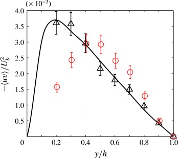
Figure 10 shows the variation of Reynolds shear stress along the wall bisector. The data have been normalised by the square of the bulk velocity. Since only the value of local friction velocity $(u_{{\it\tau}})$ at the wall midpoint is available in this experiment, normalising by $u_{{\it\tau}}^{2}$ will not provide a true picture of Reynolds shear stress distribution. The data for $Re=2230$ is in good agreement with DNS. At $Re=1203$ , Reynolds shear stress can be observed to be lower for $y/h<0.4$ . There is also a shift in location of the maximum away from the duct wall. As the duct centre is approached, Reynolds shear stress drops to zero for both flows as it must due to symmetry.

Figure 10.

Variation of Reynolds shear stress along the wall bisector: ○ (red) experiment at $Re=1203$ ; ▵, experiment at $Re=2230$ ; ——, DNS of Gavrilakis (Reference Gavrilakis1992) at $Re=2205$ .