


1 Introduction
The evaporation time of a drop brought into contact with a hot solid plate strongly depends on the solid temperature. For drops in contact with the plate (sessile drops), this time decreases with increasing plate temperature, until a sudden increase is observed. The temperature at which this increase happens is referred to as the Leidenfrost temperature
 $T_{L}$
(Boerhaave Reference Boerhaave1732; Leidenfrost Reference Leidenfrost1756). The increase is caused by the formation of a vapour film under the drop. The film separates the drop from the hot plate and the generated vapour is escaping radially from underneath the drop (see figure 1). The viscous flow induces an over-pressure, strong enough to maintain the drop levitating above the plate (Wachters, Bonne & van Nouhuis Reference Wachters, Bonne and van Nouhuis1966; Snoeijer, Brunet & Eggers Reference Snoeijer, Brunet and Eggers2009; Quéré Reference Quéré2013). The film also limits the heat transfer towards the drop, resulting in a strongly reduced evaporation and thus an increased lifetime of the drop (Biance, Clanet & Quéré Reference Biance, Clanet and Quéré2003). Then, increasing the plate temperature further above
$T_{L}$
(Boerhaave Reference Boerhaave1732; Leidenfrost Reference Leidenfrost1756). The increase is caused by the formation of a vapour film under the drop. The film separates the drop from the hot plate and the generated vapour is escaping radially from underneath the drop (see figure 1). The viscous flow induces an over-pressure, strong enough to maintain the drop levitating above the plate (Wachters, Bonne & van Nouhuis Reference Wachters, Bonne and van Nouhuis1966; Snoeijer, Brunet & Eggers Reference Snoeijer, Brunet and Eggers2009; Quéré Reference Quéré2013). The film also limits the heat transfer towards the drop, resulting in a strongly reduced evaporation and thus an increased lifetime of the drop (Biance, Clanet & Quéré Reference Biance, Clanet and Quéré2003). Then, increasing the plate temperature further above
 $T_{L}$
results again in a decrease in the lifetime of the drop. In many cooling applications, like quenching processes, superconductor cooling, heat exchangers and metal processing, the manifestation of the Leidenfrost effect is rather unfavourable as the intended cooling performance becomes inadequate. Therefore, the study of how
$T_{L}$
results again in a decrease in the lifetime of the drop. In many cooling applications, like quenching processes, superconductor cooling, heat exchangers and metal processing, the manifestation of the Leidenfrost effect is rather unfavourable as the intended cooling performance becomes inadequate. Therefore, the study of how
 $T_{L}$
depends on both the liquid and the solid material (Baumeister & Simon Reference Baumeister and Simon1973; Emmerson Reference Emmerson1975) and roughness (Bernardin & Mudawar Reference Bernardin and Mudawar1999; Kim et al.
Reference Kim, Truong, Buongiorno and Hu2011; Vakarelski et al.
Reference Vakarelski, Patankar, Marston, Chan and Thoroddsen2012) is of great importance.
$T_{L}$
depends on both the liquid and the solid material (Baumeister & Simon Reference Baumeister and Simon1973; Emmerson Reference Emmerson1975) and roughness (Bernardin & Mudawar Reference Bernardin and Mudawar1999; Kim et al.
Reference Kim, Truong, Buongiorno and Hu2011; Vakarelski et al.
Reference Vakarelski, Patankar, Marston, Chan and Thoroddsen2012) is of great importance.
Schematic illustration of a Leidenfrost drop on a heated plate. The drop remains levitated by the vapour generated in the vapour film under the drop and escaping radially.

The evaporation of a Leidenfrost drop requires (latent) heat, which is taken from the plate. To estimate whether or not this influences the plate temperature, one can compare the residence time with the characteristic cooling time scale of the plate (Baumeister & Simon Reference Baumeister and Simon1973), ranging from milliseconds to seconds. When the residence time of the drop is short (impacting drops), most solids exhibit isothermal conditions and remain at the initial plate temperature (Kim et al. Reference Kim, Truong, Buongiorno and Hu2011; Tran et al. Reference Tran, Staat, Prosperetti, Sun and Lohse2012; Staat et al. Reference Staat, Tran, Geerdink, Riboux, Sun, Gordillo and Lohse2015; Shirota et al. Reference Shirota, van Limbeek, Sun, Prosperetti and Lohse2016). Some plate materials however do show a signature of local cooling, despite the short exposure time to the evaporating drop (Tran et al. Reference Tran, Staat, Susarrey-Arce, Foertsch, van Houselt, Gardeniers, Prosperetti, Lohse and Sun2013; Nair et al. Reference Nair, Staat, Tran, van Houselt, Prosperetti, Lohse and Sun2014; van Limbeek et al. Reference van Limbeek, Shirota, Sleutel, Sun, Prosperetti and Lohse2016). However, if the residence time is of the order of seconds (sessile drops), these materials are subject to a more substantial cooling by the evaporating drop and only good thermal conductors such as copper still behave isothermally (Baumeister & Simon Reference Baumeister and Simon1973). When constantly feeding the drops, the system becomes time independent, i.e. all dynamical processes reach their steady-state regime and even a good thermal conducting plate can cool down slightly. In the study of the Leidenfrost effect, the cooling of the plate is often neglected as little quantitative data are available. Therefore, assuming the heater set point to be the actual temperature under the drop results in those cases in a non-negligible temperature (and evaporation rate) overestimation. For proper modelling of Leidenfrost drops and the interpretation of experiments, the understanding of the cooling of the plate is therefore of great importance.
Some studies focused on measuring the cooling by integrating thermocouples into the solid plate (Aziz & Chandra Reference Aziz and Chandra2000). However, this technique is intrusive and limited by the finite size of the thermocouples. Furthermore, the technique only results in a local (point) measurement and does not provide the complete temperature field.
In this study we use interferometry to measure the three-dimensional temperature field in a quartz plate which is cooled by an evaporating Leidenfrost drop. The technique is an indirect method to measure temperature, concentration or pressure fields by detecting minute variations in the refractive index (Zehnder Reference Zehnder1891; Mach Reference Mach1892). Our measurements are based on the fact that the refractive index of a solid changes with temperature, which yields a change in the optical path length. From the generated fringe patterns, obtained by a Mach–Zehnder interferometer, we can measure these changes and obtain the entire temperature field in a non-intrusive way.
To reconstruct the three-dimensional temperature field from a single interferometric projection, we develop a novel Abel inversion method, which presumes the temperature field to be an axisymmetric solution of the steady-state heat equation (i.e. the Laplace equation) inside the plate. On the one hand, these experimental data, and in particular the measured temperature distribution at the plate surface, can directly be used in Leidenfrost drop modelling, which generally amounts to the gas phase only, as for an isothermal plate (Sobac et al. Reference Sobac, Rednikov, Dorbolo and Colinet2014). This enables calculating the distribution of heat (and evaporation) fluxes and vapour film thicknesses. On the other hand, these experimental data are also crucial for validating a more complete Leidenfrost model, which includes heat conduction in the solid, and which is developed and validated here. It allows us to explore the role of solid material properties beyond experimental possibilities. Based on our findings we distinguish four different limiting regimes, characterised by two non-dimensional numbers: a Biot-like number indicating whether or not the cooling of the plate is significant, and a geometric parameter describing the global shape of the fields. Finally, we give insight into how the scaling laws proposed for isothermal substrates are modified in the case of poor thermal conducting plates.
2 Experimental set-up and methods
2.1 Experimental set-up
Figure 2 shows a schematic illustration of the experimental set-up. A Leidenfrost drop is created by placing a drop of ethanol on top of a hot solid plate with a temperature well above the boiling point of ethanol (
 $T_{b}=79\,^{\circ }\text{C}$
). The substrate is a rectangular quartz plate of dimensions
$T_{b}=79\,^{\circ }\text{C}$
). The substrate is a rectangular quartz plate of dimensions
 $15\times 30\times 4.5$
mm
$15\times 30\times 4.5$
mm
 $^{3}$
(width
$^{3}$
(width
 $W$
$W$
 $\times$
length
$\times$
length
 $\times$
height
$\times$
height
 $H_{s}$
) placed above a brass element, which coupled with a heater, a control loop feedback controller and a thermocouple, ensures a constant imposed temperature at the bottom of the plate
$H_{s}$
) placed above a brass element, which coupled with a heater, a control loop feedback controller and a thermocouple, ensures a constant imposed temperature at the bottom of the plate
 $T_{imp}$
. It is worth noting that quartz is a relatively poor thermal conductor, with a thermal conductivity
$T_{imp}$
. It is worth noting that quartz is a relatively poor thermal conductor, with a thermal conductivity
 $k_{s}=1.4~\text{W}~\text{m}^{-1}~\text{K}^{-1}$
. The drop is fed at a constant rate from a glass needle (
$k_{s}=1.4~\text{W}~\text{m}^{-1}~\text{K}^{-1}$
. The drop is fed at a constant rate from a glass needle (
 $250~\unicode[STIX]{x03BC}\text{m}$
inner diameter,
$250~\unicode[STIX]{x03BC}\text{m}$
inner diameter,
 $362~\unicode[STIX]{x03BC}\text{m}$
outer diameter) connected to a syringe pump. The needle was placed at 0.5 mm from the substrate for all experiments to ensure its tip to remain inside the drop. The feeding rate allows to control the drop radius
$362~\unicode[STIX]{x03BC}\text{m}$
outer diameter) connected to a syringe pump. The needle was placed at 0.5 mm from the substrate for all experiments to ensure its tip to remain inside the drop. The feeding rate allows to control the drop radius
 $R$
(as viewed from the top). Since quartz is transparent, one can utilise a Mach–Zehnder interferometer (see the figure 2
b) in order to visualise and measure the three-dimensional temperature field inside the plate, making use of the temperature dependence of its refractive index. This interferometer reveals optical path-length differences between the reference beam and the measurement beam, the latter one passing through our plate. The fringes resulting from combining the two beams are recorded using a camera (Photron SA7). A He–Ne laser (
$R$
(as viewed from the top). Since quartz is transparent, one can utilise a Mach–Zehnder interferometer (see the figure 2
b) in order to visualise and measure the three-dimensional temperature field inside the plate, making use of the temperature dependence of its refractive index. This interferometer reveals optical path-length differences between the reference beam and the measurement beam, the latter one passing through our plate. The fringes resulting from combining the two beams are recorded using a camera (Photron SA7). A He–Ne laser (
 $\unicode[STIX]{x1D706}=633~\text{nm}$
) is used as a collimated light source. The beam quality is improved by a spatial filter (consisting of a
$\unicode[STIX]{x1D706}=633~\text{nm}$
) is used as a collimated light source. The beam quality is improved by a spatial filter (consisting of a
 $f=7.5~\text{mm}$
aspheric focusing lens, a
$f=7.5~\text{mm}$
aspheric focusing lens, a
 $15~\unicode[STIX]{x03BC}\text{m}$
pinhole and a
$15~\unicode[STIX]{x03BC}\text{m}$
pinhole and a
 $f=100~\text{mm}$
plano-convex collimating lens) to remove the spatially varying intensity noise of the laser beam. The used system also expands the beam to ensure illumination of the complete quartz substrate. The interferometric set-up operates in the finite-fringe-width mode (i.e. with a imposed spatial carrier fringe, see § 2.2 and appendix A) to reduce the influence of noise and eliminate ambiguities in post-processing. The steps to obtain the temperature field from the interferograms will be explained in the following subsection.
$f=100~\text{mm}$
plano-convex collimating lens) to remove the spatially varying intensity noise of the laser beam. The used system also expands the beam to ensure illumination of the complete quartz substrate. The interferometric set-up operates in the finite-fringe-width mode (i.e. with a imposed spatial carrier fringe, see § 2.2 and appendix A) to reduce the influence of noise and eliminate ambiguities in post-processing. The steps to obtain the temperature field from the interferograms will be explained in the following subsection.
Schematic illustration of the experimental set-up (a) and the top view of all the optical parts of the Mach–Zehnder interferometer (b). The laser beam in (a) is orthogonal to the drawing plane and points towards the reader.

2.2 Data processing
Figure 3 shows a typical interferometry experiment with an ethanol Leidenfrost drop of size
 $R_{max}=1.4~\text{mm}$
and heater temperature
$R_{max}=1.4~\text{mm}$
and heater temperature
 $T_{imp}=330\,^{\circ }\text{C}$
. The various figures show different steps in the data processing, to be discussed in this subsection.
$T_{imp}=330\,^{\circ }\text{C}$
. The various figures show different steps in the data processing, to be discussed in this subsection.
Leidenfrost interferometry experiment with an ethanol drop (
 $R\sim \ell _{c}$
,
$R\sim \ell _{c}$
,
 $T_{imp}=330\,^{\circ }\text{C}$
), with interferogram
$T_{imp}=330\,^{\circ }\text{C}$
), with interferogram
 $I_{t}$
(a), magnitude
$I_{t}$
(a), magnitude
 $M_{t}$
and (wrapped) phase
$M_{t}$
and (wrapped) phase
 $\unicode[STIX]{x1D713}_{t}$
(b), background corrected magnitude
$\unicode[STIX]{x1D713}_{t}$
(b), background corrected magnitude
 $M$
and phase
$M$
and phase
 $\unicode[STIX]{x1D713}$
(c) and the reconstructed temperature field
$\unicode[STIX]{x1D713}$
(c) and the reconstructed temperature field
 $T(y,z)$
and drop contour (d). The wrapped phase is presented between
$T(y,z)$
and drop contour (d). The wrapped phase is presented between
 $-\unicode[STIX]{x03C0}$
(black) and
$-\unicode[STIX]{x03C0}$
(black) and
 $\unicode[STIX]{x03C0}$
(white) for (b,c). All images are on the same scale.
$\unicode[STIX]{x03C0}$
(white) for (b,c). All images are on the same scale.

The interferogram
 $I_{t}$
(figure 3
a) is decomposed into its phase
$I_{t}$
(figure 3
a) is decomposed into its phase
 $\unicode[STIX]{x1D713}_{t}$
and magnitude
$\unicode[STIX]{x1D713}_{t}$
and magnitude
 $M_{t}$
(figure 3
b) with a Fourier transform technique (Plotkowski, Hung & Gerhart Reference Plotkowski, Hung and Gerhart1985; Matthys et al.
Reference Matthys, Gilbert, Dudderar and Koenig1988; Kreis Reference Kreis2005). Since all interferograms resulting from experiments are subject to some noise which distorts the analysis process, a bandpass filter is used to remove low frequency background intensity variation of the laser beam and high frequency noise, a procedure made possible by the present use of the finite-fringe mode (appendix A). A second advantage of the present mode over the infinite-fringe-width mode (i.e. without imposing a spatial carrier fringe) is its ability of detecting smaller phase variations and the unambiguous determination of the slope of phase changes.
$M_{t}$
(figure 3
b) with a Fourier transform technique (Plotkowski, Hung & Gerhart Reference Plotkowski, Hung and Gerhart1985; Matthys et al.
Reference Matthys, Gilbert, Dudderar and Koenig1988; Kreis Reference Kreis2005). Since all interferograms resulting from experiments are subject to some noise which distorts the analysis process, a bandpass filter is used to remove low frequency background intensity variation of the laser beam and high frequency noise, a procedure made possible by the present use of the finite-fringe mode (appendix A). A second advantage of the present mode over the infinite-fringe-width mode (i.e. without imposing a spatial carrier fringe) is its ability of detecting smaller phase variations and the unambiguous determination of the slope of phase changes.
The temperature gradient in the substrate also makes the substrate appear to be displaced slightly (of the order of 0.1 mm) due to the refraction of the light. This apparent translation is determined by cross-correlating the magnitude image
 $M_{t}$
with a magnitude image from a reference interferogram taken at room temperature. The magnitude is divided by the reference magnitude to obtain the magnitude image
$M_{t}$
with a magnitude image from a reference interferogram taken at room temperature. The magnitude is divided by the reference magnitude to obtain the magnitude image
 $M$
(figure 3
c). The drop contour is obtained from this image with the Canny edge detection algorithm (Canny Reference Canny1986), from which the drop size
$M$
(figure 3
c). The drop contour is obtained from this image with the Canny edge detection algorithm (Canny Reference Canny1986), from which the drop size
 $R$
and the vapour film radius
$R$
and the vapour film radius
 $R_{c}$
are extracted.
$R_{c}$
are extracted.
The phase from the reference interferogram is subtracted to isolate the phase change
 $\unicode[STIX]{x1D713}$
due to the temperature change (figure 3
c). This removes disturbances by the optical system such as inhomogeneities of the substrate width
$\unicode[STIX]{x1D713}$
due to the temperature change (figure 3
c). This removes disturbances by the optical system such as inhomogeneities of the substrate width
 $W$
(along the direction of the laser beam), and other optical distortions.
$W$
(along the direction of the laser beam), and other optical distortions.
To obtain the absolute phase difference
 $\unicode[STIX]{x1D719}$
we need to unwrap the wrapped phase
$\unicode[STIX]{x1D719}$
we need to unwrap the wrapped phase
 $\unicode[STIX]{x1D713}\in [-\unicode[STIX]{x03C0},\unicode[STIX]{x03C0}]$
. We use the unwrapping algorithm from Herráez et al. to unwrap the phase images (Herráez et al.
Reference Herráez, Burton, Lalor and Gdeisat2002; van der Walt et al.
Reference van der Walt, Schönberger, Nunez-Iglesias, Boulogne, Warner, Yager, Gouillart and Yu2014), which excels in preventing the propagation of errors from local noise.
$\unicode[STIX]{x1D713}\in [-\unicode[STIX]{x03C0},\unicode[STIX]{x03C0}]$
. We use the unwrapping algorithm from Herráez et al. to unwrap the phase images (Herráez et al.
Reference Herráez, Burton, Lalor and Gdeisat2002; van der Walt et al.
Reference van der Walt, Schönberger, Nunez-Iglesias, Boulogne, Warner, Yager, Gouillart and Yu2014), which excels in preventing the propagation of errors from local noise.
Let
 $x$
,
$x$
,
 $y$
and
$y$
and
 $z$
be the Cartesian coordinates along the width, length and height of the quartz plate, respectively. The laser beam propagates in the
$z$
be the Cartesian coordinates along the width, length and height of the quartz plate, respectively. The laser beam propagates in the
 $x$
direction, while
$x$
direction, while
 $(y,z)$
is the plane of the field of view. The interferometric phase
$(y,z)$
is the plane of the field of view. The interferometric phase
 $\unicode[STIX]{x1D719}(y,z)$
then depends on the refractive index
$\unicode[STIX]{x1D719}(y,z)$
then depends on the refractive index
 $n(x,y,z)$
and the laser wavelength
$n(x,y,z)$
and the laser wavelength
 $\unicode[STIX]{x1D706}$
as
$\unicode[STIX]{x1D706}$
as
 $$\begin{eqnarray}\unicode[STIX]{x1D719}(y,z)=\frac{2\unicode[STIX]{x03C0}}{\unicode[STIX]{x1D706}}\int \infty -\infty \unicode[STIX]{x0394}n(x,y,z)\,dx.\end{eqnarray}$$
Here
 $\unicode[STIX]{x0394}n=n-n_{0}$
, while
$\unicode[STIX]{x0394}n=n-n_{0}$
, while
 $n_{0}$
is chosen to be the refractive index value at the ambient temperature
$n_{0}$
is chosen to be the refractive index value at the ambient temperature
 $T_{0}$
. Since the refractive index of fused quartz increases linearly with temperature,
$T_{0}$
. Since the refractive index of fused quartz increases linearly with temperature,
 $\unicode[STIX]{x0394}n=\text{d}n/\text{d}T\unicode[STIX]{x0394}T$
, we can thus relate the change in phase to the change in temperature, such that (2.1) becomes
$\unicode[STIX]{x0394}n=\text{d}n/\text{d}T\unicode[STIX]{x0394}T$
, we can thus relate the change in phase to the change in temperature, such that (2.1) becomes
 $$\begin{eqnarray}\unicode[STIX]{x1D719}(y,z)=\frac{2\unicode[STIX]{x03C0}}{\unicode[STIX]{x1D706}}\frac{\text{d}n}{\text{d}T}\int \infty -\infty \unicode[STIX]{x0394}T_{s}(x,y,z)\,dx,\end{eqnarray}$$
where
 $T_{s}(x,y,z)$
is the temperature field in the solid substrate (quartz plate), while
$T_{s}(x,y,z)$
is the temperature field in the solid substrate (quartz plate), while
 $\unicode[STIX]{x0394}T_{s}=T_{s}-T_{0}$
. A detailed description of our calibration experiment can be found in appendix B, where we obtained
$\unicode[STIX]{x0394}T_{s}=T_{s}-T_{0}$
. A detailed description of our calibration experiment can be found in appendix B, where we obtained
 $\text{d}n/\text{d}T=(1.20\pm 0.01)\times 10^{-5}~\text{K}^{-1}$
, which is in the range of values measured for fused quartz with the method of minimum deviation at
$\text{d}n/\text{d}T=(1.20\pm 0.01)\times 10^{-5}~\text{K}^{-1}$
, which is in the range of values measured for fused quartz with the method of minimum deviation at
 $\unicode[STIX]{x1D706}=633~\text{nm}$
(Malitson Reference Malitson1965; Toyoda & Yabe Reference Toyoda and Yabe1983). This experiment was also used to determine how the temperature field depended on the heater temperature in the absence of a drop for different heater set points.
$\unicode[STIX]{x1D706}=633~\text{nm}$
(Malitson Reference Malitson1965; Toyoda & Yabe Reference Toyoda and Yabe1983). This experiment was also used to determine how the temperature field depended on the heater temperature in the absence of a drop for different heater set points.
The largest source of deviation in our measurements is potentially due to neglecting the heating of air around the plate, which results in an underestimation of the change in refractive index in the quartz. However, the refractive index of air decreases with increasing temperature, with
 $\text{d}n/\text{d}T$
of the order of
$\text{d}n/\text{d}T$
of the order of
 $-10^{-7}~\text{K}^{-1}$
(Ciddor Reference Ciddor1996), which is two orders of magnitude smaller than the value of
$-10^{-7}~\text{K}^{-1}$
(Ciddor Reference Ciddor1996), which is two orders of magnitude smaller than the value of
 $\text{d}n/\text{d}T$
for quartz, hence we judge this influence to be negligible.
$\text{d}n/\text{d}T$
for quartz, hence we judge this influence to be negligible.
The final step is to reconstruct the three-dimensional temperature field
 $\unicode[STIX]{x0394}T_{s}(x,y,z)$
from the two-dimensional phase image
$\unicode[STIX]{x0394}T_{s}(x,y,z)$
from the two-dimensional phase image
 $\unicode[STIX]{x1D719}(y,z)$
by Abel inversion (figure 3
d) assuming the field to be essentially axisymmetric, i.e.
$\unicode[STIX]{x1D719}(y,z)$
by Abel inversion (figure 3
d) assuming the field to be essentially axisymmetric, i.e.
 $\unicode[STIX]{x0394}T_{s}(r,z)$
with
$\unicode[STIX]{x0394}T_{s}(r,z)$
with
 $r=\sqrt{x^{2}+y^{2}}$
. The temperature field
$r=\sqrt{x^{2}+y^{2}}$
. The temperature field
 $\unicode[STIX]{x0394}T_{s}(r,z)$
is then usually obtained using the inverse Abel transform of
$\unicode[STIX]{x0394}T_{s}(r,z)$
is then usually obtained using the inverse Abel transform of
 $\unicode[STIX]{x1D719}(y,z)$
. However, since this procedure is sensitive to noise and exhibits diverging behaviour near the origin, it is not quite suitable to be used on our experimental data. Therefore, we propose a new inversion method based on the basis function expansion method (Dribinski et al.
Reference Dribinski, Ossadtchi, Mandelshtam and Reisler2002) for expressing the experimentally obtained phase field
$\unicode[STIX]{x1D719}(y,z)$
. However, since this procedure is sensitive to noise and exhibits diverging behaviour near the origin, it is not quite suitable to be used on our experimental data. Therefore, we propose a new inversion method based on the basis function expansion method (Dribinski et al.
Reference Dribinski, Ossadtchi, Mandelshtam and Reisler2002) for expressing the experimentally obtained phase field
 $\unicode[STIX]{x1D719}(y,z)$
as a series expansion in terms of axisymmetric modes of
$\unicode[STIX]{x1D719}(y,z)$
as a series expansion in terms of axisymmetric modes of
 $\unicode[STIX]{x0394}T_{s}(r,z)$
. The two expansions will obviously be related by means of (2.2).
$\unicode[STIX]{x0394}T_{s}(r,z)$
. The two expansions will obviously be related by means of (2.2).
 $\unicode[STIX]{x0394}T_{s}(r,z)$
is governed by the steady-state heat (Laplace) equation
$\unicode[STIX]{x0394}T_{s}(r,z)$
is governed by the steady-state heat (Laplace) equation
 $\unicode[STIX]{x1D6FB}^{2}(\unicode[STIX]{x0394}T_{s})=0$
. Thus, a set of Fourier–Bessel functions can be used for
$\unicode[STIX]{x1D6FB}^{2}(\unicode[STIX]{x0394}T_{s})=0$
. Thus, a set of Fourier–Bessel functions can be used for
 $\unicode[STIX]{x0394}T_{s}(r,z)$
, see appendix C, which when integrated according to (2.2) yields the corresponding set of functions for
$\unicode[STIX]{x0394}T_{s}(r,z)$
, see appendix C, which when integrated according to (2.2) yields the corresponding set of functions for
 $\unicode[STIX]{x1D719}(y,z)$
. The coefficients of the series expansions for
$\unicode[STIX]{x1D719}(y,z)$
. The coefficients of the series expansions for
 $\unicode[STIX]{x0394}T_{s}(r,z)$
and
$\unicode[STIX]{x0394}T_{s}(r,z)$
and
 $\unicode[STIX]{x1D719}(y,z)$
herewith clearly coincide. They are determined by fitting the experimental data for
$\unicode[STIX]{x1D719}(y,z)$
herewith clearly coincide. They are determined by fitting the experimental data for
 $\unicode[STIX]{x1D719}(y,z)$
. Once the coefficients are known, the temperature field
$\unicode[STIX]{x1D719}(y,z)$
. Once the coefficients are known, the temperature field
 $\unicode[STIX]{x0394}T_{s}(r,z)$
gets fully determined too from its own series expansion up to a constant. We fix this constant such that the average temperature on the bottom of the substrate is equal to the heater set-point temperature
$\unicode[STIX]{x0394}T_{s}(r,z)$
gets fully determined too from its own series expansion up to a constant. We fix this constant such that the average temperature on the bottom of the substrate is equal to the heater set-point temperature
 $T_{imp}$
.
$T_{imp}$
.
3 Formulation of the theoretical model
In order to model the experimental situation, we consider an axisymmetric Leidenfrost drop levitating over a hot solid substrate. The present model is aimed at predicting the quasi-steady state of such a drop (the slowest process being its evaporation), including both its geometry and a possible cooling of the substrate. The drop geometry is modelled by numerically matching the hydrostatic equilibrium shape of a superhydrophobic drop (for the upper part) with the lubrication equation solution for the vapour film underlying the drop (for the bottom part), quite similarly to Sobac et al. (Reference Sobac, Rednikov, Dorbolo and Colinet2014). However, unlike Sobac et al. (Reference Sobac, Rednikov, Dorbolo and Colinet2014), the substrate is no longer considered isothermal, and its cooling is accounted for by solving a heat transfer problem therein. As in the experiment, the substrate is assumed to consist of a horizontal plate (height
 $H_{s}$
) with the temperature kept constant at its bottom surface.
$H_{s}$
) with the temperature kept constant at its bottom surface.
Let us first focus on the shape of the drop, following Sobac et al. (Reference Sobac, Rednikov, Dorbolo and Colinet2014). The upper part of the drop is assumed to be an equilibrium shape, for which the Laplace pressure locally balances (up to a constant) the hydrostatic pressure. This simply reads
 $$\begin{eqnarray}\unicode[STIX]{x1D6FE}\unicode[STIX]{x1D705}+\unicode[STIX]{x1D70C}_{\ell }g(z-z_{top})=\unicode[STIX]{x1D6FE}\unicode[STIX]{x1D705}_{top},\end{eqnarray}$$
where
 $\unicode[STIX]{x1D70C}_{\ell }$
is the liquid density,
$\unicode[STIX]{x1D70C}_{\ell }$
is the liquid density,
 $\unicode[STIX]{x1D6FE}$
is the surface tension and
$\unicode[STIX]{x1D6FE}$
is the surface tension and
 $g$
is the gravitational acceleration. Here,
$g$
is the gravitational acceleration. Here,
 $\unicode[STIX]{x1D705}$
is the local curvature of the drop surface (a function of the drop shape and its derivatives), while
$\unicode[STIX]{x1D705}$
is the local curvature of the drop surface (a function of the drop shape and its derivatives), while
 $\unicode[STIX]{x1D705}_{top}$
(curvature at the top of the drop,
$\unicode[STIX]{x1D705}_{top}$
(curvature at the top of the drop,
 $z=z_{top}$
) is a free parameter controlling the drop size. For a given value of the top curvature
$z=z_{top}$
) is a free parameter controlling the drop size. For a given value of the top curvature
 $\unicode[STIX]{x1D705}_{top}$
, numerically integrating this differential equation from the symmetry axis yields the corresponding equilibrium shape and in particular the value of the drop radius
$\unicode[STIX]{x1D705}_{top}$
, numerically integrating this differential equation from the symmetry axis yields the corresponding equilibrium shape and in particular the value of the drop radius
 $R=R(\unicode[STIX]{x1D705}_{top})$
, defined in figure 1. Inversely, for any given
$R=R(\unicode[STIX]{x1D705}_{top})$
, defined in figure 1. Inversely, for any given
 $R$
, one unambiguously finds the corresponding equilibrium shape and
$R$
, one unambiguously finds the corresponding equilibrium shape and
 $\unicode[STIX]{x1D705}_{top}$
. Yet, the shape is hereby determined just up to a vertical shift, for the value of
$\unicode[STIX]{x1D705}_{top}$
. Yet, the shape is hereby determined just up to a vertical shift, for the value of
 $z_{top}$
can fully be calculated only upon the consideration of the underlying vapour film, as is explained hereafter.
$z_{top}$
can fully be calculated only upon the consideration of the underlying vapour film, as is explained hereafter.
This ‘upper equilibrium drop’ solution is assumed to be valid up to a (patching) point located at
 $r=R_{p}$
near the exit from the vapour film, where non-equilibrium effects of evaporation and viscous pressure losses in the vapour flow now need to be taken into account. In this ‘vapour layer region’
$r=R_{p}$
near the exit from the vapour film, where non-equilibrium effects of evaporation and viscous pressure losses in the vapour flow now need to be taken into account. In this ‘vapour layer region’
 $0<r<R_{p}$
, the thickness of the vapour film
$0<r<R_{p}$
, the thickness of the vapour film
 $h(r)$
and its slopes
$h(r)$
and its slopes
 $h^{\prime }(r)$
are assumed to be small enough so as to use the lubrication approximation (in particular,
$h^{\prime }(r)$
are assumed to be small enough so as to use the lubrication approximation (in particular,
 $h\ll R$
and
$h\ll R$
and
 $|h^{\prime }|\ll 1$
). The gas itself is assumed to be composed of pure vapour (no air) and incompressible. Then, discarding possible motions inside the drop, which is a feature of all similar models developed thus far (Wachters et al.
Reference Wachters, Bonne and van Nouhuis1966; Snoeijer et al.
Reference Snoeijer, Brunet and Eggers2009; Pomeau et al.
Reference Pomeau, Le Berre, Celestini and Frisch2012; Sobac et al.
Reference Sobac, Rednikov, Dorbolo and Colinet2014), the excess pressure (over the ambient one) in the vapour film is found from the normal stress balance at the drop surface as
$|h^{\prime }|\ll 1$
). The gas itself is assumed to be composed of pure vapour (no air) and incompressible. Then, discarding possible motions inside the drop, which is a feature of all similar models developed thus far (Wachters et al.
Reference Wachters, Bonne and van Nouhuis1966; Snoeijer et al.
Reference Snoeijer, Brunet and Eggers2009; Pomeau et al.
Reference Pomeau, Le Berre, Celestini and Frisch2012; Sobac et al.
Reference Sobac, Rednikov, Dorbolo and Colinet2014), the excess pressure (over the ambient one) in the vapour film is found from the normal stress balance at the drop surface as
 $P_{v}=\unicode[STIX]{x1D6FE}\unicode[STIX]{x1D705}_{top}+\unicode[STIX]{x1D70C}_{l}g(z_{top}-h)-\unicode[STIX]{x1D6FE}\unicode[STIX]{x1D705}$
. This excess pressure drives a Stokes flow (the maximum Reynolds number for the parameters of the present study was found to be around 0.5, for more details see appendix D) with a volumetric flux
$P_{v}=\unicode[STIX]{x1D6FE}\unicode[STIX]{x1D705}_{top}+\unicode[STIX]{x1D70C}_{l}g(z_{top}-h)-\unicode[STIX]{x1D6FE}\unicode[STIX]{x1D705}$
. This excess pressure drives a Stokes flow (the maximum Reynolds number for the parameters of the present study was found to be around 0.5, for more details see appendix D) with a volumetric flux
 $\boldsymbol{q}_{v}=-(\unicode[STIX]{x1D735}P_{v}/12\unicode[STIX]{x1D707}_{v})h^{3}$
, where
$\boldsymbol{q}_{v}=-(\unicode[STIX]{x1D735}P_{v}/12\unicode[STIX]{x1D707}_{v})h^{3}$
, where
 $\unicode[STIX]{x1D707}_{v}$
is the vapour dynamic viscosity. Note the coefficient
$\unicode[STIX]{x1D707}_{v}$
is the vapour dynamic viscosity. Note the coefficient
 $1/12$
in the mobility factor, reflecting of the no-slip conditions imposed at both the drop and solid interfaces. The no-slip condition at the drop interface results from the large viscosity ratio between the vapour and the drop and is generally assumed in the literature (Wachters et al.
Reference Wachters, Bonne and van Nouhuis1966; Biance et al.
Reference Biance, Clanet and Quéré2003; Quéré Reference Quéré2013; Sobac et al.
Reference Sobac, Rednikov, Dorbolo and Colinet2014). Assuming that heat is predominantly transferred by conduction across the film (the Péclet number is estimated to be approximately 0.4, for more details see appendix D), the local evaporation flux at the interface is expressed as
$1/12$
in the mobility factor, reflecting of the no-slip conditions imposed at both the drop and solid interfaces. The no-slip condition at the drop interface results from the large viscosity ratio between the vapour and the drop and is generally assumed in the literature (Wachters et al.
Reference Wachters, Bonne and van Nouhuis1966; Biance et al.
Reference Biance, Clanet and Quéré2003; Quéré Reference Quéré2013; Sobac et al.
Reference Sobac, Rednikov, Dorbolo and Colinet2014). Assuming that heat is predominantly transferred by conduction across the film (the Péclet number is estimated to be approximately 0.4, for more details see appendix D), the local evaporation flux at the interface is expressed as
 ${\mathcal{J}}={\mathcal{L}}^{-1}k_{v}\unicode[STIX]{x0394}T/h$
, where
${\mathcal{J}}={\mathcal{L}}^{-1}k_{v}\unicode[STIX]{x0394}T/h$
, where
 $k_{v}$
is the vapour thermal conductivity,
$k_{v}$
is the vapour thermal conductivity,
 ${\mathcal{L}}$
is the latent heat of vaporisation,
${\mathcal{L}}$
is the latent heat of vaporisation,
 $\unicode[STIX]{x0394}T=T_{s\unicode[STIX]{x1D6F4}}-T_{sat}$
is the superheat and
$\unicode[STIX]{x0394}T=T_{s\unicode[STIX]{x1D6F4}}-T_{sat}$
is the superheat and
 $T_{s\unicode[STIX]{x1D6F4}}$
is the temperature field of the substrate surface underneath the drop. Finally, the steady-state vapour mass conservation under the thin-film hypothesis reads
$T_{s\unicode[STIX]{x1D6F4}}$
is the temperature field of the substrate surface underneath the drop. Finally, the steady-state vapour mass conservation under the thin-film hypothesis reads
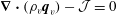 $\unicode[STIX]{x1D735}\boldsymbol{\cdot }(\unicode[STIX]{x1D70C}_{v}\boldsymbol{q}_{v})-{\mathcal{J}}=0$
(at steady state), where
$\unicode[STIX]{x1D735}\boldsymbol{\cdot }(\unicode[STIX]{x1D70C}_{v}\boldsymbol{q}_{v})-{\mathcal{J}}=0$
(at steady state), where
 $\unicode[STIX]{x1D70C}_{v}$
is the vapour density. Combining these results and assuming the axial symmetry yields the following lubrication equation for the film thickness
$\unicode[STIX]{x1D70C}_{v}$
is the vapour density. Combining these results and assuming the axial symmetry yields the following lubrication equation for the film thickness
 $$\begin{eqnarray}\frac{1}{12}\frac{1}{r}\frac{\unicode[STIX]{x2202}}{\unicode[STIX]{x2202}r}\left(\frac{\unicode[STIX]{x1D70C}_{v}}{\unicode[STIX]{x1D707}_{v}}h^{3}r\frac{\unicode[STIX]{x2202}}{\unicode[STIX]{x2202}r}(\unicode[STIX]{x1D70C}_{l}gh+\unicode[STIX]{x1D6FE}\unicode[STIX]{x1D705})\right)-\frac{k_{v}\unicode[STIX]{x0394}T}{{\mathcal{L}}h}=0,\end{eqnarray}$$
where the curvature
 $\unicode[STIX]{x1D705}$
is given by
$\unicode[STIX]{x1D705}$
is given by
 $$\begin{eqnarray}\unicode[STIX]{x1D705}=\frac{\displaystyle \frac{\unicode[STIX]{x2202}^{2}h}{\unicode[STIX]{x2202}r^{2}}+\displaystyle \frac{1}{r}\left(1+\left(\frac{\unicode[STIX]{x2202}h}{\unicode[STIX]{x2202}r}\right)^{2}\right)\frac{\unicode[STIX]{x2202}h}{\unicode[STIX]{x2202}r}}{\displaystyle \left(1+\left(\frac{\unicode[STIX]{x2202}h}{\unicode[STIX]{x2202}r}\right)^{2}\right)^{3/2}},\end{eqnarray}$$
expressed in full (unlinearised) form to improve the accuracy of the patching of the solution of (3.2) with the top part of the drop, as expressed by (3.1).
The system is characterised by large spatial temperature variations, the typical values of
 $\unicode[STIX]{x0394}T$
being generally rather comparable with the absolute temperature itself. As the liquid and gas properties are temperature dependent, a relevant question is therefore at what temperature they should be evaluated in our formulation. This is more straightforward for the liquid properties: as the drop supposedly remains at (or near to)
$\unicode[STIX]{x0394}T$
being generally rather comparable with the absolute temperature itself. As the liquid and gas properties are temperature dependent, a relevant question is therefore at what temperature they should be evaluated in our formulation. This is more straightforward for the liquid properties: as the drop supposedly remains at (or near to)
 $T_{sat}$
, they are just taken at
$T_{sat}$
, they are just taken at
 $T_{sat}$
. As for the vapour properties, a simplified treatment similar to Sobac et al. (Reference Sobac, Rednikov, Dorbolo and Colinet2014) will be used, evaluating physical properties locally at the mean temperature of the vapour film,
$T_{sat}$
. As for the vapour properties, a simplified treatment similar to Sobac et al. (Reference Sobac, Rednikov, Dorbolo and Colinet2014) will be used, evaluating physical properties locally at the mean temperature of the vapour film,
 $(T_{s\unicode[STIX]{x1D6F4}}(r)+T_{sat})/2$
. Thus, the effect of a temperature variation at the top of the substrate due to the cooling enters here not only through a position-dependent superheat
$(T_{s\unicode[STIX]{x1D6F4}}(r)+T_{sat})/2$
. Thus, the effect of a temperature variation at the top of the substrate due to the cooling enters here not only through a position-dependent superheat
 $\unicode[STIX]{x0394}T(r)$
, but also through the vapour properties which vary along
$\unicode[STIX]{x0394}T(r)$
, but also through the vapour properties which vary along
 $r$
. The vapour properties themselves are calculated as in Sobac et al. (Reference Sobac, Talbot, Haut, Rednikov and Colinet2015b
). For instance, at a temperature of
$r$
. The vapour properties themselves are calculated as in Sobac et al. (Reference Sobac, Talbot, Haut, Rednikov and Colinet2015b
). For instance, at a temperature of
 $200\,^{\circ }\text{C}$
, the values of the vapour mass density, dynamic viscosity and thermal conductivity of ethanol vapour are
$200\,^{\circ }\text{C}$
, the values of the vapour mass density, dynamic viscosity and thermal conductivity of ethanol vapour are
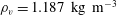 $\unicode[STIX]{x1D70C}_{v}=1.187~\text{kg}~\text{m}^{-3}$
,
$\unicode[STIX]{x1D70C}_{v}=1.187~\text{kg}~\text{m}^{-3}$
,
 $\unicode[STIX]{x1D707}_{v}=1.436\times 10^{-5}~\text{Pa}~\text{s}$
and
$\unicode[STIX]{x1D707}_{v}=1.436\times 10^{-5}~\text{Pa}~\text{s}$
and
 $k_{v}=0.023~\text{W}~\text{m}^{-1}~\text{K}^{-1}$
, respectively.
$k_{v}=0.023~\text{W}~\text{m}^{-1}~\text{K}^{-1}$
, respectively.
Four boundary conditions are needed to supplement (3.2) and (3.3): the symmetry conditions at
 $r=0$
, i.e.
$r=0$
, i.e.
 $h^{\prime }(0)=0$
and
$h^{\prime }(0)=0$
and
 $\unicode[STIX]{x1D705}^{\prime }(0)=0$
, while at
$\unicode[STIX]{x1D705}^{\prime }(0)=0$
, while at
 $r=R_{p}$
the solution must match with the earlier obtained upper equilibrium shape of the drop, i.e. we require the continuity of
$r=R_{p}$
the solution must match with the earlier obtained upper equilibrium shape of the drop, i.e. we require the continuity of
 $h^{\prime }(r)$
and of
$h^{\prime }(r)$
and of
 $\unicode[STIX]{x1D705}(r)$
. The continuity of
$\unicode[STIX]{x1D705}(r)$
. The continuity of
 $h(r)$
itself here merely amounts to finding the appropriate vertical shift of the upper equilibrium shape, i.e. to determining the value of
$h(r)$
itself here merely amounts to finding the appropriate vertical shift of the upper equilibrium shape, i.e. to determining the value of
 $z_{top}$
.
$z_{top}$
.
The temperature distribution
 $T_{s\unicode[STIX]{x1D6F4}}(r)$
at the top of the solid substrate is obtained by solving the heat conduction equation in the plate coupled with (3.2). Assuming quasi-steadiness and a constant thermal conductivity
$T_{s\unicode[STIX]{x1D6F4}}(r)$
at the top of the solid substrate is obtained by solving the heat conduction equation in the plate coupled with (3.2). Assuming quasi-steadiness and a constant thermal conductivity
 $k_{s}$
of the solid, the temperature field
$k_{s}$
of the solid, the temperature field
 $T_{s}(r,z)$
in the solid is governed by the axisymmetric Laplace equation
$T_{s}(r,z)$
in the solid is governed by the axisymmetric Laplace equation
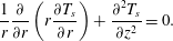 $$\begin{eqnarray}\frac{1}{r}\frac{\unicode[STIX]{x2202}}{\unicode[STIX]{x2202}r}\left(r\frac{\unicode[STIX]{x2202}T_{s}}{\unicode[STIX]{x2202}r}\right)+\frac{\unicode[STIX]{x2202}^{2}T_{s}}{\unicode[STIX]{x2202}z^{2}}=0.\end{eqnarray}$$
The following boundary conditions finally close the problem: the symmetry condition
 $\unicode[STIX]{x2202}_{r}T_{s}=0$
at
$\unicode[STIX]{x2202}_{r}T_{s}=0$
at
 $r=0$
, an imposed temperature at the substrate bottom, i.e.
$r=0$
, an imposed temperature at the substrate bottom, i.e.
 $T_{s}=T_{imp}$
at
$T_{s}=T_{imp}$
at
 $z=-H_{s}$
, and heat fluxes continuity at
$z=-H_{s}$
, and heat fluxes continuity at
 $r=R_{s}$
and
$r=R_{s}$
and
 $z=0$
. At the plate sides, an experimental evaluation of heat losses to the air due to convection proved them to be negligible. Consequently, an insulating condition will be imposed thereat, i.e.
$z=0$
. At the plate sides, an experimental evaluation of heat losses to the air due to convection proved them to be negligible. Consequently, an insulating condition will be imposed thereat, i.e.
 $\unicode[STIX]{x2202}_{r}T_{s}=0$
at
$\unicode[STIX]{x2202}_{r}T_{s}=0$
at
 $r=R_{s}$
. For mathematical simplicity, the plate is assumed to be cylindrical with radius
$r=R_{s}$
. For mathematical simplicity, the plate is assumed to be cylindrical with radius
 $R_{s}$
in the model, while it is rectangular in the experiment.
$R_{s}$
in the model, while it is rectangular in the experiment.
 $R_{s}$
is taken as half the plate width, i.e.
$R_{s}$
is taken as half the plate width, i.e.
 $R_{s}=7.5~\text{mm}$
. This is expected to have just a minor impact on the results given that the drop remains small enough compared to the horizontal extent of the plate.
$R_{s}=7.5~\text{mm}$
. This is expected to have just a minor impact on the results given that the drop remains small enough compared to the horizontal extent of the plate.
At the top of the plate (
 $z=0$
, see figure 1), two zones are distinguished depending on the position with respect to the patching point. Right below the drop (
$z=0$
, see figure 1), two zones are distinguished depending on the position with respect to the patching point. Right below the drop (
 $0<r\leqslant R_{p}$
), the heat flux lost by the substrate is equal to the heat flux consumed by the drop for its evaporation,
$0<r\leqslant R_{p}$
), the heat flux lost by the substrate is equal to the heat flux consumed by the drop for its evaporation,
 ${\mathcal{J}}L=k_{v}(r)(T_{s\unicode[STIX]{x1D6F4}}(r)-T_{sat})/h(r)$
. Outside the ‘patching perimeter’ (
${\mathcal{J}}L=k_{v}(r)(T_{s\unicode[STIX]{x1D6F4}}(r)-T_{sat})/h(r)$
. Outside the ‘patching perimeter’ (
 $R_{p}<r<R_{s}$
), the heat loss by the substrate is due to natural convection in the air, here described by Newton’s law of cooling
$R_{p}<r<R_{s}$
), the heat loss by the substrate is due to natural convection in the air, here described by Newton’s law of cooling
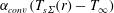 $\unicode[STIX]{x1D6FC}_{conv}(T_{s\unicode[STIX]{x1D6F4}}(r)-T_{\infty })$
, where
$\unicode[STIX]{x1D6FC}_{conv}(T_{s\unicode[STIX]{x1D6F4}}(r)-T_{\infty })$
, where
 $T_{\infty }$
is the ambient temperature far from the plate and
$T_{\infty }$
is the ambient temperature far from the plate and
 $\unicode[STIX]{x1D6FC}_{conv}$
is the convective heat transfer coefficient. The value of
$\unicode[STIX]{x1D6FC}_{conv}$
is the convective heat transfer coefficient. The value of
 $\unicode[STIX]{x1D6FC}_{conv}$
is determined from the experiments in the absence of the drop as
$\unicode[STIX]{x1D6FC}_{conv}$
is determined from the experiments in the absence of the drop as
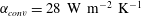 $\unicode[STIX]{x1D6FC}_{conv}=28~\text{W}~\text{m}^{-2}~\text{K}^{-1}$
(see § 4.2). Clearly, with the heat distribution defined in this way the flux generally proves to be discontinuous at
$\unicode[STIX]{x1D6FC}_{conv}=28~\text{W}~\text{m}^{-2}~\text{K}^{-1}$
(see § 4.2). Clearly, with the heat distribution defined in this way the flux generally proves to be discontinuous at
 $r=R_{p}$
. For numerical convenience, we use an exponential smoothing to yield
$r=R_{p}$
. For numerical convenience, we use an exponential smoothing to yield
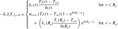 $$\begin{eqnarray}-k_{s}\unicode[STIX]{x2202}_{z}T_{s}|_{z=0}=\left\{\begin{array}{@{}ll@{}}\displaystyle k_{v}(r)\frac{T_{s}(r)-T_{sat}}{h(r)}\quad & \text{for }r\leqslant R_{p}\\ \displaystyle \unicode[STIX]{x1D6FC}_{conv}(T_{s}(r)-T_{\infty })(1-\text{e}^{B(R_{p}-r)})\quad & \\ \displaystyle \quad +\,\left(k_{v}(R_{p})\frac{T_{s}(R_{p})-T_{sat}}{h(R_{p})}\right)\text{e}^{B(R_{p}-r)}\quad & \text{for }r>R_{p},\end{array}\right.\end{eqnarray}$$
where
 $B$
is a parameter whose value is determined by demanding in addition continuous differentiability at
$B$
is a parameter whose value is determined by demanding in addition continuous differentiability at
 $r=R_{p}$
.
$r=R_{p}$
.
The problem given by (3.2)–(3.4) with the formulated boundary conditions is discretised in a standard way by second-order finite differences. The resulting nonlinear algebraic system of equations for the values of
 $h$
,
$h$
,
 $\unicode[STIX]{x1D705}$
,
$\unicode[STIX]{x1D705}$
,
 $T_{s}$
at the grid points as well as the values of
$T_{s}$
at the grid points as well as the values of
 $z_{top}$
and
$z_{top}$
and
 $B$
is solved by the Newton–Raphson method. It is checked a posteriori that the choice of the patching point
$B$
is solved by the Newton–Raphson method. It is checked a posteriori that the choice of the patching point
 $R_{p}$
has no significant influence on the results.
$R_{p}$
has no significant influence on the results.
Temperature field inside the quartz plate under static Leidenfrost drops of ethanol of different sizes. For each presented case, the numerical result (left half) is juxtaposed with the experimental measurement (right half) for comparison. On the latter, the arrows indicate the direction and relative magnitude of the heat flux. The imposed temperature at the bottom of the substrate is
 $T_{imp}=330\,^{\circ }\text{C}$
. The lengths are normalised with the capillary length
$T_{imp}=330\,^{\circ }\text{C}$
. The lengths are normalised with the capillary length
 $\ell _{c}$
, i.e. 1.56 mm for ethanol at
$\ell _{c}$
, i.e. 1.56 mm for ethanol at
 $T_{sat}$
.
$T_{sat}$
.

Profiles of the substrate surface temperature (a) and of the vapour film thickness (b) for
 $T_{imp}=330\,^{\circ }\text{C}$
and four different drop sizes. Three cases are shown in panel (b) for each drop size according to the way the substrate surface temperature profile is handled in the model: fully isothermal substrate at
$T_{imp}=330\,^{\circ }\text{C}$
and four different drop sizes. Three cases are shown in panel (b) for each drop size according to the way the substrate surface temperature profile is handled in the model: fully isothermal substrate at
 $T_{imp}$
(dashed lines), borrowed from the experiment (solid lines), and calculated in the framework of the full model (dot-dashed lines). The top panel presents both experimental and numerical results, the latter calculated from the full model.
$T_{imp}$
(dashed lines), borrowed from the experiment (solid lines), and calculated in the framework of the full model (dot-dashed lines). The top panel presents both experimental and numerical results, the latter calculated from the full model.

Finally, one has to note that, aside the above presented ‘full’ model, a ‘partial’ modelling will also be tested here. It consists in skipping the computation of the substrate temperature field and rather borrowing the measured substrate temperature distribution
 $T_{s\unicode[STIX]{x1D6F4}}(r)$
from the experiment, using it directly in (3.2) for the calculation of the vapour film thickness profile.
$T_{s\unicode[STIX]{x1D6F4}}(r)$
from the experiment, using it directly in (3.2) for the calculation of the vapour film thickness profile.
4 Results and discussion
4.1 Experimental observations and numerical validation
Figure 4 shows the temperature fields inside the quartz plate for four different drop sizes and for an imposed temperature at the plate bottom
 $T_{imp}=330\,^{\circ }\text{C}$
. For each size, the left half of the diagram shows the numerical results while the right half corresponds to the experimental data. A strong cooling of the substrate underneath the Leidenfrost drop is observed. The cooling proves to be roughly one third of the ‘ideal’ superheat
$T_{imp}=330\,^{\circ }\text{C}$
. For each size, the left half of the diagram shows the numerical results while the right half corresponds to the experimental data. A strong cooling of the substrate underneath the Leidenfrost drop is observed. The cooling proves to be roughly one third of the ‘ideal’ superheat
 $T_{imp}-T_{sat}\simeq 250~\text{K}$
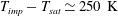
, and generally depends on the heater temperature. The temperature field in the plate also depends on the drop size, as observed in figure 4. As the drop becomes larger, the global shape of the temperature field appears to change from a locally rather spherical shape in the drop vicinity to a more one-dimensional field (as will be discussed in more detail in § 4.2).
$T_{imp}-T_{sat}\simeq 250~\text{K}$
, and generally depends on the heater temperature. The temperature field in the plate also depends on the drop size, as observed in figure 4. As the drop becomes larger, the global shape of the temperature field appears to change from a locally rather spherical shape in the drop vicinity to a more one-dimensional field (as will be discussed in more detail in § 4.2).
The experimental and numerical results appear to compare fairly well as highlighted by the iso-temperature contours in figure 4 and the temperature profiles at the top of the plate in figure 5(a). In the latter figure, even if the agreement is overall quite satisfactory, the data reveal a systematic mismatch of 15 % between experimental and numerical results and further deviate in the centre. In particular, the numerically predicted maximum substrate cooling (with respect to
 $T_{imp}=330\,^{\circ }\text{C}$
) is here approximately 80 K, while the measured one is approximately 95 K. On the one hand, the mentioned mismatch can partly be attributed to the uncertainty in our calibration. On the other hand, the deviation in the centre may further be related to oscillatory lateral motions of the Leidenfrost drops around the needle. These are actually always present in our experiments and likely to give rise to higher evaporation rates, and hence to stronger substrate cooling, as a larger area of the plate is affected by the evaporating drop. Besides, evaporation rate determination based only on the vapour film (ignoring the contribution of the upper part of the drop), even if it indeed remains the principal contribution, is nonetheless known to systematically underestimate the global evaporation rates (Biance et al.
Reference Biance, Clanet and Quéré2003; Sobac et al.
Reference Sobac, Talbot, Haut, Rednikov and Colinet2015b
; Maquet et al.
Reference Maquet, Sobac, Darbois-Texier, Duchesne, Brandenbourger, Rednikov, Colinet and Dorbolo2016).
$T_{imp}=330\,^{\circ }\text{C}$
) is here approximately 80 K, while the measured one is approximately 95 K. On the one hand, the mentioned mismatch can partly be attributed to the uncertainty in our calibration. On the other hand, the deviation in the centre may further be related to oscillatory lateral motions of the Leidenfrost drops around the needle. These are actually always present in our experiments and likely to give rise to higher evaporation rates, and hence to stronger substrate cooling, as a larger area of the plate is affected by the evaporating drop. Besides, evaporation rate determination based only on the vapour film (ignoring the contribution of the upper part of the drop), even if it indeed remains the principal contribution, is nonetheless known to systematically underestimate the global evaporation rates (Biance et al.
Reference Biance, Clanet and Quéré2003; Sobac et al.
Reference Sobac, Talbot, Haut, Rednikov and Colinet2015b
; Maquet et al.
Reference Maquet, Sobac, Darbois-Texier, Duchesne, Brandenbourger, Rednikov, Colinet and Dorbolo2016).
At the same time, this moderate discrepancy is not deemed to be due to the presence of the needle in the experiment (and the absence thereof in the modelling), as a numerical study revealed that the bottom shape of the drop is barely affected by the presence of the needle for a given drop radius (as viewed from the top) in the range considered here (see appendix E). It is interesting to note that in our studied parameter regime the minimum substrate temperature due to the cooling is practically unaffected by the drop size, either experimentally or theoretically. Moreover, the theoretical results highlight that the substrate surface temperature drop is maximum right below the neck, i.e. at the location where the vapour film is the thinnest. This feature is apparently smoothed out in the extraction of the experimental temperature profiles at the substrate surface but can still be observed from figure 4 in terms of the heat flux, which at the top of the substrate proves indeed to be maximum just at the neck location.
The cooling of the substrate due to the presence of a Leidenfrost drop is expected to affect the vapour film underneath the drop as compared to the corresponding isothermal substrate situation. As the cooling implies
 $T_{s\unicode[STIX]{x1D6F4}}<T_{imp}$
, with the local superheat
$T_{s\unicode[STIX]{x1D6F4}}<T_{imp}$
, with the local superheat
 $T_{s\unicode[STIX]{x1D6F4}}-T_{sat}$
then being lower than its ideal value
$T_{s\unicode[STIX]{x1D6F4}}-T_{sat}$
then being lower than its ideal value
 $T_{imp}-T_{sat}$
, one can expect a reduction in both the evaporation rates and vapour film thicknesses (and hence an increase in the lifetime of the drops). This can already be qualitatively confirmed based on the scaling laws established by Sobac et al. (Reference Sobac, Rednikov, Dorbolo and Colinet2014) for isothermal substrates, according to which
$T_{imp}-T_{sat}$
, one can expect a reduction in both the evaporation rates and vapour film thicknesses (and hence an increase in the lifetime of the drops). This can already be qualitatively confirmed based on the scaling laws established by Sobac et al. (Reference Sobac, Rednikov, Dorbolo and Colinet2014) for isothermal substrates, according to which
 $h\sim (T_{s\unicode[STIX]{x1D6F4}}-T_{sat})^{1/3}$
in the neck region and
$h\sim (T_{s\unicode[STIX]{x1D6F4}}-T_{sat})^{1/3}$
in the neck region and
 $h\sim (T_{s\unicode[STIX]{x1D6F4}}-T_{sat})^{1/6}$
in the vapour pocket, both tending to decrease with diminishing superheat. The global evaporation rate of the drop,
$h\sim (T_{s\unicode[STIX]{x1D6F4}}-T_{sat})^{1/6}$
in the vapour pocket, both tending to decrease with diminishing superheat. The global evaporation rate of the drop,
 $(-{\dot{M}})$
, as mostly determined by evaporation through the vapour film, is given by
$(-{\dot{M}})$
, as mostly determined by evaporation through the vapour film, is given by
 $(-{\dot{M}})=(2\unicode[STIX]{x03C0}/{\mathcal{L}})\int _{0}^{R_{p}}(k_{v}(T_{s\unicode[STIX]{x1D6F4}}-T_{sat})/h)r\,\text{d}r$
, and is then also expected to decrease. The relatively small exponents in the mentioned scaling laws indicate that the vapour film thickness is apparently not modified too drastically as compared to the isothermal substrate case, but a more essential effect can be expected, quite conversely, in terms of the evaporation rates. These speculations are partly confirmed in figure 5(b) that shows the numerically predicted profiles of the vapour layer for the cases considered in figure 4. The results of the full model (dot-dashed lines) are compared to the corresponding results for an isothermal substrate with
$(-{\dot{M}})=(2\unicode[STIX]{x03C0}/{\mathcal{L}})\int _{0}^{R_{p}}(k_{v}(T_{s\unicode[STIX]{x1D6F4}}-T_{sat})/h)r\,\text{d}r$
, and is then also expected to decrease. The relatively small exponents in the mentioned scaling laws indicate that the vapour film thickness is apparently not modified too drastically as compared to the isothermal substrate case, but a more essential effect can be expected, quite conversely, in terms of the evaporation rates. These speculations are partly confirmed in figure 5(b) that shows the numerically predicted profiles of the vapour layer for the cases considered in figure 4. The results of the full model (dot-dashed lines) are compared to the corresponding results for an isothermal substrate with
 $T_{s\unicode[STIX]{x1D6F4}}\equiv T_{imp}$
(dashed lines). The results obtained by considering in the model the experimental temperature profile at the top of the substrate instead of fully solving for the temperature field in the plate are also provided (solid lines). One observes a close agreement between the full model and the one based on
$T_{s\unicode[STIX]{x1D6F4}}\equiv T_{imp}$
(dashed lines). The results obtained by considering in the model the experimental temperature profile at the top of the substrate instead of fully solving for the temperature field in the plate are also provided (solid lines). One observes a close agreement between the full model and the one based on
 $T_{s\unicode[STIX]{x1D6F4}}$
adopted from the experiment. In contrast, these numerical and ‘experimental’ vapour film thicknesses manifest quite an appreciable reduction of approximately 17 % relative to the isothermal substrate case. As far as the global evaporation rates are concerned, the reduction is estimated to be approximately 26 %, which points to the importance of incorporating the effect of cooling into Leidenfrost modelling for not so highly conductive substrates.
$T_{s\unicode[STIX]{x1D6F4}}$
adopted from the experiment. In contrast, these numerical and ‘experimental’ vapour film thicknesses manifest quite an appreciable reduction of approximately 17 % relative to the isothermal substrate case. As far as the global evaporation rates are concerned, the reduction is estimated to be approximately 26 %, which points to the importance of incorporating the effect of cooling into Leidenfrost modelling for not so highly conductive substrates.
4.2 Cooling strength criterion
As already mentioned in § 3, the measurement of the temperature field in our quartz plate in the absence of any drop enables estimating the value of the heat transfer coefficient
 $\unicode[STIX]{x1D6FC}_{conv}$
assuming heat losses at the top of the plate to be describable by Newton’s cooling law
$\unicode[STIX]{x1D6FC}_{conv}$
assuming heat losses at the top of the plate to be describable by Newton’s cooling law
 $\unicode[STIX]{x1D6FC}_{conv}(T_{s\unicode[STIX]{x1D6F4}}-T_{\infty })$
. Whether or not any significant temperature gradient emerges in the plate as a result can be characterised by an appropriate Biot number (essentially a dimensionless form of the heat transfer coefficient). The heat balance across the plate surface can be written as
$\unicode[STIX]{x1D6FC}_{conv}(T_{s\unicode[STIX]{x1D6F4}}-T_{\infty })$
. Whether or not any significant temperature gradient emerges in the plate as a result can be characterised by an appropriate Biot number (essentially a dimensionless form of the heat transfer coefficient). The heat balance across the plate surface can be written as
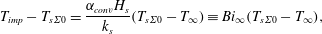 $$\begin{eqnarray}T_{imp}-T_{s\unicode[STIX]{x1D6F4}0}=\frac{\unicode[STIX]{x1D6FC}_{conv}H_{s}}{k_{s}}(T_{s\unicode[STIX]{x1D6F4}0}-T_{\infty })\equiv Bi_{\infty }(T_{s\unicode[STIX]{x1D6F4}0}-T_{\infty }),\end{eqnarray}$$
where
 $Bi_{\infty }$
is the Biot number quantifying heat losses to the surroundings. Hence
$Bi_{\infty }$
is the Biot number quantifying heat losses to the surroundings. Hence
 $$\begin{eqnarray}T_{s\unicode[STIX]{x1D6F4}0}=\frac{T_{imp}+Bi_{\infty }T_{\infty }}{1+Bi_{\infty }}\quad \text{with }Bi_{\infty }=\frac{\unicode[STIX]{x1D6FC}_{conv}H_{s}}{k_{s}},\end{eqnarray}$$
where the subscript ‘0’ refers to the temperature in the absence of the drop. The smaller
 $Bi_{\infty }$
, the more the heat transfer through the plate is limited by heat exchange with the surroundings without any noticeable temperature difference in the plate. It is interesting to note that, in principle, one cannot here go too far into the opposite limit of extremely poor thermal conducting substrates (
$Bi_{\infty }$
, the more the heat transfer through the plate is limited by heat exchange with the surroundings without any noticeable temperature difference in the plate. It is interesting to note that, in principle, one cannot here go too far into the opposite limit of extremely poor thermal conducting substrates (
 $Bi_{\infty }\gg 1$
) due to the risk of
$Bi_{\infty }\gg 1$
) due to the risk of
 $T_{s\unicode[STIX]{x1D6F4}0}$
actually falling below
$T_{s\unicode[STIX]{x1D6F4}0}$
actually falling below
 $T_{sat}=79\,^{\circ }\text{C}$
(for ethanol) so that effectively no superheating exists. In our experimental set-up, with
$T_{sat}=79\,^{\circ }\text{C}$
(for ethanol) so that effectively no superheating exists. In our experimental set-up, with
 $k_{s}=1.4~\text{W}~\text{m}^{-1}~\text{K}$
,
$k_{s}=1.4~\text{W}~\text{m}^{-1}~\text{K}$
,
 $H_{s}=4.5~\text{mm}$
,
$H_{s}=4.5~\text{mm}$
,
 $T_{imp}=330\,^{\circ }\text{C}$
and
$T_{imp}=330\,^{\circ }\text{C}$
and
 $T_{\infty }=22\,^{\circ }\text{C}$
,
$T_{\infty }=22\,^{\circ }\text{C}$
,
 $T_{imp}-T_{s\unicode[STIX]{x1D6F4}0}=25\,^{\circ }\text{C}$
was measured (in the absence of any drop). Thus, we obtain
$T_{imp}-T_{s\unicode[STIX]{x1D6F4}0}=25\,^{\circ }\text{C}$
was measured (in the absence of any drop). Thus, we obtain
 $\unicode[STIX]{x1D6FC}_{conv}\approx 28~\text{W}~\text{m}^{-2}~\text{K}$
, and hence
$\unicode[STIX]{x1D6FC}_{conv}\approx 28~\text{W}~\text{m}^{-2}~\text{K}$
, and hence
 $Bi_{\infty }\approx 0.09$
.
$Bi_{\infty }\approx 0.09$
.
Following the same reasoning as above, but now in an approximate way for the case when the plate is exposed to a relatively small (
 $R\lesssim H_{s}$
) Leidenfrost drop,
$R\lesssim H_{s}$
) Leidenfrost drop,
 $\unicode[STIX]{x1D6FC}_{conv}$
in (4.2) must be replaced by
$\unicode[STIX]{x1D6FC}_{conv}$
in (4.2) must be replaced by
 $k_{v}/h$
,
$k_{v}/h$
,
 $T_{\infty }$
by
$T_{\infty }$
by
 $T_{sat}$
,
$T_{sat}$
,
 $T_{imp}$
by
$T_{imp}$
by
 $T_{s\unicode[STIX]{x1D6F4}0}$
(‘background’ substrate temperature (for a small droplet) due to cooling by the ambient, determined by (4.2)) and
$T_{s\unicode[STIX]{x1D6F4}0}$
(‘background’ substrate temperature (for a small droplet) due to cooling by the ambient, determined by (4.2)) and
 $H_{s}$
by
$H_{s}$
by
 $R$
. Then the counterpart of (4.2) is found to be
$R$
. Then the counterpart of (4.2) is found to be
 $$\begin{eqnarray}T_{s\unicode[STIX]{x1D6F4}}\sim \frac{T_{s\unicode[STIX]{x1D6F4}0}+Bi_{d}T_{sat}}{1+Bi_{d}}\quad \text{with }Bi_{d}=\frac{k_{v}R}{2k_{s}h}\;(\text{for }R\lesssim H_{s}).\end{eqnarray}$$
Here also note a geometrical factor
 $2$
(area ratio of the hemisphere and the corresponding circle) introduced into the expression for the droplet-associated Biot number
$2$
(area ratio of the hemisphere and the corresponding circle) introduced into the expression for the droplet-associated Biot number
 $Bi_{d}$
due to the mentioned local sphericity of the temperature field in the considered case
$Bi_{d}$
due to the mentioned local sphericity of the temperature field in the considered case
 $R\lesssim H_{s}$
(cf. table 1, left-hand column). The value of
$R\lesssim H_{s}$
(cf. table 1, left-hand column). The value of
 $Bi_{d}$
once again indicates whether a significant substrate cooling is incurred, now associated with our Leidenfrost drop: the cooling is negligible for
$Bi_{d}$
once again indicates whether a significant substrate cooling is incurred, now associated with our Leidenfrost drop: the cooling is negligible for
 $Bi_{d}\ll 1$
and appreciable for
$Bi_{d}\ll 1$
and appreciable for
 $Bi_{d}\sim 1$
.
$Bi_{d}\sim 1$
.
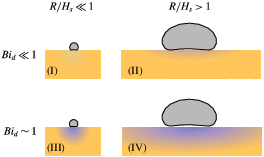
Schematic illustrating the four different regimes for the temperature field in the substrate underneath a Leidenfrost drop, which depend on the ratio between the drop radius
 $R$
and the substrate height
$R$
and the substrate height
 $H_{s}$
as well as on the Biot number
$H_{s}$
as well as on the Biot number
 $Bi_{d}$
(incorporating the substrate thermal conductivity). Regimes (II) and (IV) are characterised by a more one-dimensional profile, while in the other limit, regimes (I) and (III) resemble locally a spherical profile from a point source. Since for regimes (III) and (IV) the Biot number is not small, a significant cooling by the evaporating drop is expected, while for regimes (I) and (II) the substrate remains largely isothermal.
$Bi_{d}$
(incorporating the substrate thermal conductivity). Regimes (II) and (IV) are characterised by a more one-dimensional profile, while in the other limit, regimes (I) and (III) resemble locally a spherical profile from a point source. Since for regimes (III) and (IV) the Biot number is not small, a significant cooling by the evaporating drop is expected, while for regimes (I) and (II) the substrate remains largely isothermal.
Biot number values for the cases of figure 6 and the estimates of
 $T_{s\unicode[STIX]{x1D6F4}}$
, cf. equations (4.2)–(4.4), which can be compared to
$T_{s\unicode[STIX]{x1D6F4}}$
, cf. equations (4.2)–(4.4), which can be compared to
 $\bar{T}_{s\unicode[STIX]{x1D6F4}}$
. Here the bar denotes the area averages underneath the droplet obtained by numerical resolution of the full model and
$\bar{T}_{s\unicode[STIX]{x1D6F4}}$
. Here the bar denotes the area averages underneath the droplet obtained by numerical resolution of the full model and
 $k_{v}$
is evaluated at the temperature
$k_{v}$
is evaluated at the temperature
 $(\bar{T}_{s\unicode[STIX]{x1D6F4}}+T_{sat})/2$
. The superscripts ‘(I)’ and ‘(II)’ refer, exclusively within this table, to the results for
$(\bar{T}_{s\unicode[STIX]{x1D6F4}}+T_{sat})/2$
. The superscripts ‘(I)’ and ‘(II)’ refer, exclusively within this table, to the results for
 $R\lesssim H_{s}$
and
$R\lesssim H_{s}$
and
 $R\gtrsim H_{s}$
given by (4.3) and (4.4), respectively. Results presented in italic represent values obtained using the improper equation given its radius.
$R\gtrsim H_{s}$
given by (4.3) and (4.4), respectively. Results presented in italic represent values obtained using the improper equation given its radius.

For larger drops (
 $R\gtrsim H_{s}$
), however, the temperature field is more one-dimensional (cf. table 1, right-hand column), and the result (4.2) should now be adapted by merely replacing
$R\gtrsim H_{s}$
), however, the temperature field is more one-dimensional (cf. table 1, right-hand column), and the result (4.2) should now be adapted by merely replacing
 $\unicode[STIX]{x1D6FC}_{conv}$
by
$\unicode[STIX]{x1D6FC}_{conv}$
by
 $k_{v}/h$
and
$k_{v}/h$
and
 $T_{\infty }$
by
$T_{\infty }$
by
 $T_{sat}$
. Then we obtain an estimation
$T_{sat}$
. Then we obtain an estimation
 $$\begin{eqnarray}T_{s\unicode[STIX]{x1D6F4}}\sim \frac{T_{imp}+Bi_{d}T_{sat}}{1+Bi_{d}}\quad \text{with }Bi_{d}=\frac{k_{v}H_{s}}{k_{s}h}\;(\text{for }R\gtrsim H_{s}).\end{eqnarray}$$
To illustrate the behaviour of the substrate temperature field in terms of the introduced Biot numbers, a parametric study has been carried out by varying the substrate thermal conductivity for a number of droplet sizes. The computation results for the profiles of
 $T_{s\unicode[STIX]{x1D6F4}}(r)$
based on the full model are shown in figure 6, while the Biot numbers corresponding to each case are estimated in table 2. In these estimations,
$T_{s\unicode[STIX]{x1D6F4}}(r)$
based on the full model are shown in figure 6, while the Biot numbers corresponding to each case are estimated in table 2. In these estimations,
 $\bar{T}_{s\unicode[STIX]{x1D6F4}}$
and
$\bar{T}_{s\unicode[STIX]{x1D6F4}}$
and
 $\bar{h}$
are the averages of the corresponding quantities, obtained from the full model, over the substrate surface area underneath the droplet (taken up until the outer circle where the vapour film thickness doubles relative to its value at the neck). In (4.3) and (4.4),
$\bar{h}$
are the averages of the corresponding quantities, obtained from the full model, over the substrate surface area underneath the droplet (taken up until the outer circle where the vapour film thickness doubles relative to its value at the neck). In (4.3) and (4.4),
 $h$
is taken equal to
$h$
is taken equal to
 $\bar{h}$
. Figure 6 and table 2 clearly confirm that the degree of substrate temperature uniformity and the deviations of
$\bar{h}$
. Figure 6 and table 2 clearly confirm that the degree of substrate temperature uniformity and the deviations of
 $T_{s}$
from
$T_{s}$
from
 $T_{imp}$
are well characterised by the Biot number values: comparing the average temperature for
$T_{imp}$
are well characterised by the Biot number values: comparing the average temperature for
 $r<R$
from the figure seem to correspond well to the calculated values for
$r<R$
from the figure seem to correspond well to the calculated values for
 $T_{s\unicode[STIX]{x1D6F4}}$
. For comparison, both equations are evaluated for all cases, denoting the improper ones (based on the droplet radius) in italic for comparison. Interestingly enough, the estimate (4.3) for
$T_{s\unicode[STIX]{x1D6F4}}$
. For comparison, both equations are evaluated for all cases, denoting the improper ones (based on the droplet radius) in italic for comparison. Interestingly enough, the estimate (4.3) for
 $T_{s\unicode[STIX]{x1D6F4}}$
, intended for
$T_{s\unicode[STIX]{x1D6F4}}$
, intended for
 $R\lesssim H_{s}$
, happens to work with a rather good accuracy for all cases shown in figure 6 and table 2. The estimate (4.4), intended for
$R\lesssim H_{s}$
, happens to work with a rather good accuracy for all cases shown in figure 6 and table 2. The estimate (4.4), intended for
 $R\gtrsim H_{s}$
, however yields good results just for the largest of the droplets considered.
$R\gtrsim H_{s}$
, however yields good results just for the largest of the droplets considered.
On the other hand, the case
 $R\lesssim H_{s}$
turns out to be characterised by a high degree of substrate surface temperature uniformity just underneath the droplet (cf. figure 6 and then also § 4.4), irrespective of how large the Biot number may be. This adds to the value of the estimate (4.3), which was inherently formulated disregarding such variations of
$R\lesssim H_{s}$
turns out to be characterised by a high degree of substrate surface temperature uniformity just underneath the droplet (cf. figure 6 and then also § 4.4), irrespective of how large the Biot number may be. This adds to the value of the estimate (4.3), which was inherently formulated disregarding such variations of
 $T_{s\unicode[STIX]{x1D6F4}}$
and which can now in principle be used in lieu of solving the full problem for
$T_{s\unicode[STIX]{x1D6F4}}$
and which can now in principle be used in lieu of solving the full problem for
 $T_{s}$
thus greatly simplifying the mathematical formulation (cf. also § 4.4). On the contrary, such variations of
$T_{s}$
thus greatly simplifying the mathematical formulation (cf. also § 4.4). On the contrary, such variations of
 $T_{s\unicode[STIX]{x1D6F4}}$
prove to be increasingly more important underneath larger droplets,
$T_{s\unicode[STIX]{x1D6F4}}$
prove to be increasingly more important underneath larger droplets,
 $R\gtrsim H_{s}$
, which is not surprising given a highly non-uniform local evaporation flux (due to a highly non-uniform film thickness) along the vapour layer and an increased proximity of the substrate bottom with a fixed temperature
$R\gtrsim H_{s}$
, which is not surprising given a highly non-uniform local evaporation flux (due to a highly non-uniform film thickness) along the vapour layer and an increased proximity of the substrate bottom with a fixed temperature
 $T_{imp}$
. In a further limit,
$T_{imp}$
. In a further limit,
 $R\gg H_{s}$
, the result (4.4) can rather be understood locally, at each
$R\gg H_{s}$
, the result (4.4) can rather be understood locally, at each
 $r$
, and used as such in conjunction with the film equation (3.2), which is another case of a great simplification of the overall mathematical formulation (again practically down to the level of the one in the case of an isothermal substrate). Yet we shall not further pursue this limit here, as large drops typically develop chimneys, for which the lubrication-based analysis presented here is not accurate.
$r$
, and used as such in conjunction with the film equation (3.2), which is another case of a great simplification of the overall mathematical formulation (again practically down to the level of the one in the case of an isothermal substrate). Yet we shall not further pursue this limit here, as large drops typically develop chimneys, for which the lubrication-based analysis presented here is not accurate.
Numerically determined temperature profile at the top of the substrate underneath a Leidenfrost drop for different drop sizes and thermal conductivities of the substrate.
 $H_{s}$
is taken at the value of the quartz plate height used in the experiment (
$H_{s}$
is taken at the value of the quartz plate height used in the experiment (
 $H_{s}=H_{q}=4.5~\text{mm}$
).
$H_{s}=H_{q}=4.5~\text{mm}$
).
 $T_{imp}=330\,^{\circ }\text{C}$
and
$T_{imp}=330\,^{\circ }\text{C}$
and
 $k_{q}=1.4~\text{W}~\text{m}^{-1}~\text{K}^{-1}$
, the thermal conductivity of quartz.
$k_{q}=1.4~\text{W}~\text{m}^{-1}~\text{K}^{-1}$
, the thermal conductivity of quartz.

4.3 Exploring the influence of the substrate thermal conductivity
We have seen that the strength of substrate cooling due to a Leidenfrost drop is greatly influenced by the thermal conductivity of the substrate
 $k_{s}$
. Therefore, to further explore this effect, we here carry out a parametric study by varying
$k_{s}$
. Therefore, to further explore this effect, we here carry out a parametric study by varying
 $k_{s}$
beyond the constraints of a concrete experimental set-up (in this sense modelling various substrate materials). As earlier in figure 5, we shall be interested in the profiles of both the substrate surface temperature and the vapour film thickness. It is natural to expect the cooling of the substrate to be reduced as
$k_{s}$
beyond the constraints of a concrete experimental set-up (in this sense modelling various substrate materials). As earlier in figure 5, we shall be interested in the profiles of both the substrate surface temperature and the vapour film thickness. It is natural to expect the cooling of the substrate to be reduced as
 $k_{s}$
is increased so that the isothermal limit is recovered for relatively high substrate thermal conductivities. Numerical results to test this hypothesis are shown in figure 7 for an ethanol drop with radius
$k_{s}$
is increased so that the isothermal limit is recovered for relatively high substrate thermal conductivities. Numerical results to test this hypothesis are shown in figure 7 for an ethanol drop with radius
 $R=1.37\ell _{c}$
and a quartz plate with thermal conductivity
$R=1.37\ell _{c}$
and a quartz plate with thermal conductivity
 $k_{q}=1.4~\text{W}~\text{m}^{-1}~\text{K}^{-1}$
. Indeed, increasing the thermal conductivity of the substrate is seen to rapidly lead to the isothermal regime. For
$k_{q}=1.4~\text{W}~\text{m}^{-1}~\text{K}^{-1}$
. Indeed, increasing the thermal conductivity of the substrate is seen to rapidly lead to the isothermal regime. For
 $k_{s}=10k_{q}$
, the maximum cooling is reduced from approximately 75 K to only approximately 10 K, while for
$k_{s}=10k_{q}$
, the maximum cooling is reduced from approximately 75 K to only approximately 10 K, while for
 $k_{s}\gtrsim 100k_{q}$
, no discernible cooling with respect to the imposed bottom temperature of the plate can be found within our numerical precision (panel a). With the increase in the substrate surface temperature, the evaporation rate increases as well, resulting in a thicker vapour layer as shown in panel (b).
$k_{s}\gtrsim 100k_{q}$
, no discernible cooling with respect to the imposed bottom temperature of the plate can be found within our numerical precision (panel a). With the increase in the substrate surface temperature, the evaporation rate increases as well, resulting in a thicker vapour layer as shown in panel (b).
Effect of the variation of the substrate thermal conductivity
 $k_{s}$
on the numerically predicted profiles of the substrate surface temperature (a) and the vapour film thickness (b) underneath a Leidenfrost ethanol drop of
$k_{s}$
on the numerically predicted profiles of the substrate surface temperature (a) and the vapour film thickness (b) underneath a Leidenfrost ethanol drop of
 $R=1.37\ell _{c}$
with
$R=1.37\ell _{c}$
with
 $T_{imp}=330\,^{\circ }\text{C}$
and the plate height (
$T_{imp}=330\,^{\circ }\text{C}$
and the plate height (
 $H_{s}=4.5~\text{mm}\approx 3\ell _{c}$
) as in the experiment. The value of
$H_{s}=4.5~\text{mm}\approx 3\ell _{c}$
) as in the experiment. The value of
 $k_{s}$
for the quartz used in the experiment is denoted by
$k_{s}$
for the quartz used in the experiment is denoted by
 $k_{q}$
.
$k_{q}$
.

4.4 Regression to the isothermal model
Figure 8 shows the numerically predicted profiles of the vapour layer thickness for two drop sizes and two imposed temperatures. The results of the full model (solid lines), with a numerically obtained
 $T_{s\unicode[STIX]{x1D6F4}}(r)$
, are compared to the corresponding results for an isothermal substrate taken just at a mean temperature
$T_{s\unicode[STIX]{x1D6F4}}(r)$
, are compared to the corresponding results for an isothermal substrate taken just at a mean temperature
 $\overline{T}_{s\unicode[STIX]{x1D6F4}}$
(dashed lines). Here
$\overline{T}_{s\unicode[STIX]{x1D6F4}}$
(dashed lines). Here
 $\overline{T}_{s\unicode[STIX]{x1D6F4}}$
is obtained by averaging
$\overline{T}_{s\unicode[STIX]{x1D6F4}}$
is obtained by averaging
 $T_{s\unicode[STIX]{x1D6F4}}(r)$
computed from the full model over the substrate surface area underneath the drop (up to the patching point). One observes that the predicted shapes of the vapour layer are almost identical. It means that instead of solving the full model, it would be possible to solve just the isothermal substrate model if the mentioned mean temperature could somehow be evaluated (e.g. like with (4.3) in § 4.2). This is attributed to relatively small (compared to the superheat) radial variations of
$T_{s\unicode[STIX]{x1D6F4}}(r)$
computed from the full model over the substrate surface area underneath the drop (up to the patching point). One observes that the predicted shapes of the vapour layer are almost identical. It means that instead of solving the full model, it would be possible to solve just the isothermal substrate model if the mentioned mean temperature could somehow be evaluated (e.g. like with (4.3) in § 4.2). This is attributed to relatively small (compared to the superheat) radial variations of
 $T_{s\unicode[STIX]{x1D6F4}}(r)$
underneath the drop actually occurring in the present set-up. Consequently, the results by Sobac et al. (Reference Sobac, Rednikov, Dorbolo and Colinet2014), obtained for isothermal substrates (viz. perfectly conducting plates in the present context), are expected to be valid with a reasonable precision here even for poorly conducting substrates in terms of the mean temperature
$T_{s\unicode[STIX]{x1D6F4}}(r)$
underneath the drop actually occurring in the present set-up. Consequently, the results by Sobac et al. (Reference Sobac, Rednikov, Dorbolo and Colinet2014), obtained for isothermal substrates (viz. perfectly conducting plates in the present context), are expected to be valid with a reasonable precision here even for poorly conducting substrates in terms of the mean temperature
 $\overline{T}_{s\unicode[STIX]{x1D6F4}}$
.
$\overline{T}_{s\unicode[STIX]{x1D6F4}}$
.
Numerically predicted profiles of the vapour film thickness for two drop sizes,
 $R=0.87\ell _{c}$
and
$R=0.87\ell _{c}$
and
 $R=2.28\ell _{c}$
. The results of the full model (solid lines) are compared to the corresponding results for an isothermal substrate taken at the mean substrate surface temperature underneath the drop (dashed line), the latter temperature here also calculated from the full model. For each drop size, two imposed temperatures are studied,
$R=2.28\ell _{c}$
. The results of the full model (solid lines) are compared to the corresponding results for an isothermal substrate taken at the mean substrate surface temperature underneath the drop (dashed line), the latter temperature here also calculated from the full model. For each drop size, two imposed temperatures are studied,
 $T_{imp}=330\,^{\circ }\text{C}$
(top pairs) and
$T_{imp}=330\,^{\circ }\text{C}$
(top pairs) and
 $T_{imp}=275\,^{\circ }\text{C}$
(bottom pairs), while the substrate is the quartz plate used in the experiments.
$T_{imp}=275\,^{\circ }\text{C}$
(bottom pairs), while the substrate is the quartz plate used in the experiments.

For instance, some scaling laws have been established by Sobac et al. (Reference Sobac, Rednikov, Dorbolo and Colinet2014) as far as the (minimal and maximal) vapour film thicknesses and the evaporation rates are concerned, expressed as functions of an evaporation number
 ${\mathcal{E}}$
. In particular,
${\mathcal{E}}$
. In particular,
 $h_{neck}\sim {\mathcal{E}}^{1/3}$
for the neck thickness, the neck being identified as the narrowest point of the vapour film, see e.g. figure 7(b). In the present context, such an evaporation number can just be defined in a modified way, based on
$h_{neck}\sim {\mathcal{E}}^{1/3}$
for the neck thickness, the neck being identified as the narrowest point of the vapour film, see e.g. figure 7(b). In the present context, such an evaporation number can just be defined in a modified way, based on
 $\overline{T}_{s\unicode[STIX]{x1D6F4}}$
, as follows:
$\overline{T}_{s\unicode[STIX]{x1D6F4}}$
, as follows:
 $$\begin{eqnarray}{\mathcal{E}}=\frac{\overline{k}_{v}\overline{\unicode[STIX]{x1D707}}_{v}(\overline{T}_{s\unicode[STIX]{x1D6F4}}-T_{sat})}{\unicode[STIX]{x1D6FE}\overline{\unicode[STIX]{x1D70C}}_{v}\ell _{c}{\mathcal{L}}}.\end{eqnarray}$$
The vapour properties are here evaluated at
 $(\overline{T}_{s\unicode[STIX]{x1D6F4}}+T_{sat})/2$
(i.e. in a manner similar to § 3 and to Sobac et al. (Reference Sobac, Rednikov, Dorbolo and Colinet2014)) to yield in particular
$(\overline{T}_{s\unicode[STIX]{x1D6F4}}+T_{sat})/2$
(i.e. in a manner similar to § 3 and to Sobac et al. (Reference Sobac, Rednikov, Dorbolo and Colinet2014)) to yield in particular
 $\overline{k}_{v}$
,
$\overline{k}_{v}$
,
 $\overline{\unicode[STIX]{x1D707}}_{v}$
and
$\overline{\unicode[STIX]{x1D707}}_{v}$
and
 $\overline{\unicode[STIX]{x1D70C}}_{v}$
. For example, as shown in figure 9, the neck thickness, computed from a non-isothermal substrate model (full or partial) does well observe the mentioned
$\overline{\unicode[STIX]{x1D70C}}_{v}$
. For example, as shown in figure 9, the neck thickness, computed from a non-isothermal substrate model (full or partial) does well observe the mentioned
 $1/3$
power law in terms of the hereby defined parameter
$1/3$
power law in terms of the hereby defined parameter
 ${\mathcal{E}}$
whatever the substrate conductivity, the substrate thickness and the imposed temperature. A slight scattering of points about the straight line is mainly attributed to slightly different values of
${\mathcal{E}}$
whatever the substrate conductivity, the substrate thickness and the imposed temperature. A slight scattering of points about the straight line is mainly attributed to slightly different values of
 $R$
used in the computation following different experimental runs (for which it is difficult to reproduce exactly the same
$R$
used in the computation following different experimental runs (for which it is difficult to reproduce exactly the same
 $R$
), for the proportionality factor is actually
$R$
), for the proportionality factor is actually
 $R$
-dependent (Sobac et al.
Reference Sobac, Rednikov, Dorbolo and Colinet2014).
$R$
-dependent (Sobac et al.
Reference Sobac, Rednikov, Dorbolo and Colinet2014).
The
 $1/3$
power law in terms of the evaporation number defined in (4.5) for the numerically determined neck thickness. The three circles within each (blue, black and red) set correspond, in an increasing order of
$1/3$
power law in terms of the evaporation number defined in (4.5) for the numerically determined neck thickness. The three circles within each (blue, black and red) set correspond, in an increasing order of
 ${\mathcal{E}}$
, to
${\mathcal{E}}$
, to
 $T_{imp}=220\,^{\circ }\text{C}$
and
$T_{imp}=220\,^{\circ }\text{C}$
and
 $R=1.39\ell _{c}$
, to
$R=1.39\ell _{c}$
, to
 $T_{imp}=275\,^{\circ }\text{C}$
and
$T_{imp}=275\,^{\circ }\text{C}$
and
 $R=1.314\ell _{c}$
and to
$R=1.314\ell _{c}$
and to
 $T_{imp}=330\,^{\circ }\text{C}$
and
$T_{imp}=330\,^{\circ }\text{C}$
and
 $R=1.37\ell _{c}$
, a slight scattering in the chosen
$R=1.37\ell _{c}$
, a slight scattering in the chosen
 $R$
values being due to the one in corresponding experimental realisations. The colours: blue for the overall isothermal substrates at
$R$
values being due to the one in corresponding experimental realisations. The colours: blue for the overall isothermal substrates at
 $T_{imp}$
, black for the partial model (with experimentally measured temperature profiles) and red for the full model. Crosses and pluses all correspond to the full model at
$T_{imp}$
, black for the partial model (with experimentally measured temperature profiles) and red for the full model. Crosses and pluses all correspond to the full model at
 $T_{imp}=330\,^{\circ }\text{C}$
and
$T_{imp}=330\,^{\circ }\text{C}$
and
 $R=1.37\ell _{c}$
. The crosses are for
$R=1.37\ell _{c}$
. The crosses are for
 $H_{s}=H_{q}$
and the indicated values of
$H_{s}=H_{q}$
and the indicated values of
 $k_{s}$
, while the pluses are for
$k_{s}$
, while the pluses are for
 $k_{s}=k_{q}$
and the indicated values of
$k_{s}=k_{q}$
and the indicated values of
 $H_{s}$
. Here
$H_{s}$
. Here
 $H_{q}=4.5~\text{mm}$
and
$H_{q}=4.5~\text{mm}$
and
 $k_{q}=1.4~\text{W}~\text{m}^{-1}~\text{K}^{-1}$
are the
$k_{q}=1.4~\text{W}~\text{m}^{-1}~\text{K}^{-1}$
are the
 $H_{s}$
and
$H_{s}$
and
 $k_{s}$
values of the quartz plate used in the experiments.
$k_{s}$
values of the quartz plate used in the experiments.

5 Conclusions
The present study has focused, both experimentally and theoretically, on the temperature field in the solid substrate underneath a Leidenfrost drop in the case of relatively low thermal conductivity solids such as quartz. A non-trivial feedback between substrate cooling and Leidenfrost drop characteristics has been highlighted. In the experiments, the drop is continuously fed from a needle so as to achieve an overall stationary situation. The temperature field in a quartz plate substrate is experimentally visualised by means of a Mach–Zehnder interferometer. Quite a strong local cooling of the substrate caused by a Leidenfrost (ethanol) drop was detected, which comes alongside with a non-negligible cooling due to natural convection in the air already present in the absence of any drop. For instance, a local temperature drop as large as 80 K was measured in the range of parameters investigated in this study (viz. a 4.5 mm thick quartz plate with its bottom surface maintained at
 $330\,^{\circ }\text{C}$
). This can be compared with a 30 K upper surface cooling measured in the absence of any drop, and with the intended ‘ideal’ superheat of 251 K (
$330\,^{\circ }\text{C}$
). This can be compared with a 30 K upper surface cooling measured in the absence of any drop, and with the intended ‘ideal’ superheat of 251 K (
 $=330\,^{\circ }\text{C}{-}79\,^{\circ }\text{C}$
, the ethanol boiling temperature being equal to
$=330\,^{\circ }\text{C}{-}79\,^{\circ }\text{C}$
, the ethanol boiling temperature being equal to
 $79\,^{\circ }\text{C}$
). Quite remarkably, such a maximum local cooling proved to depend only weakly on the drop size in a capillary-length range. A theoretical model has been developed in order to rationalise the experimental data and appeared to fairly well compare with the experiments, despite its simplicity. Interestingly enough, the simulations revealed the maximum substrate temperature drop to occur right underneath the neck of the vapour film, roughly coinciding with the expected maximum of heat (and evaporation) fluxes, although the experimental resolution did not prove to be sufficient to conclusively capture such a fine effect in terms of the temperature drop (though it did in terms of the local heat flux). On the other hand, the modelling somewhat underestimates (by some 15 K) the value of the temperature drop, which apparently partly goes along with a long-standing problem of underestimating the overall evaporation rates when not accounting for the contribution of the upper part of the drop, even if the contribution of the lower part (i.e. the vapour film) is indeed predominant. The simulations showed the substrate cooling to be associated with a reduction of about 17 % in the vapour film thickness and 26 % in the evaporation rate as compared with the case of an isothermal substrate (at
$79\,^{\circ }\text{C}$
). Quite remarkably, such a maximum local cooling proved to depend only weakly on the drop size in a capillary-length range. A theoretical model has been developed in order to rationalise the experimental data and appeared to fairly well compare with the experiments, despite its simplicity. Interestingly enough, the simulations revealed the maximum substrate temperature drop to occur right underneath the neck of the vapour film, roughly coinciding with the expected maximum of heat (and evaporation) fluxes, although the experimental resolution did not prove to be sufficient to conclusively capture such a fine effect in terms of the temperature drop (though it did in terms of the local heat flux). On the other hand, the modelling somewhat underestimates (by some 15 K) the value of the temperature drop, which apparently partly goes along with a long-standing problem of underestimating the overall evaporation rates when not accounting for the contribution of the upper part of the drop, even if the contribution of the lower part (i.e. the vapour film) is indeed predominant. The simulations showed the substrate cooling to be associated with a reduction of about 17 % in the vapour film thickness and 26 % in the evaporation rate as compared with the case of an isothermal substrate (at
 $330\,^{\circ }\text{C}$
) under otherwise equal settings. Thus, the Leidenfrost effect is subject to an appreciable influence of non-isothermal effects in the substrate. A parametric study was carried out in order to explore what happens for substrates with properties (thermal conductivity, size) beyond the constrains of the present experimental settings. Quite expectedly, as the thermal conductivity is increased, the isothermal substrate case is recovered, for which a Leidenfrost model like the earlier one by Sobac et al. (Reference Sobac, Rednikov, Dorbolo and Colinet2014) becomes fully sufficient. Simple criteria in terms of Biot numbers were formulated permitting to a priori estimate the expected importance of substrate cooling for any particular settings. Finally, whatever the value of the Biot number, the scaling laws for the vapour film thickness as a function of the evaporation number established elsewhere in the case of an isothermal substrate prove to remain valid here with a good accuracy if for the isothermal substrate temperature one substitutes the mean substrate surface temperature underneath the Leidenfrost drop, for which a well-working analytical estimate is provided.
$330\,^{\circ }\text{C}$
) under otherwise equal settings. Thus, the Leidenfrost effect is subject to an appreciable influence of non-isothermal effects in the substrate. A parametric study was carried out in order to explore what happens for substrates with properties (thermal conductivity, size) beyond the constrains of the present experimental settings. Quite expectedly, as the thermal conductivity is increased, the isothermal substrate case is recovered, for which a Leidenfrost model like the earlier one by Sobac et al. (Reference Sobac, Rednikov, Dorbolo and Colinet2014) becomes fully sufficient. Simple criteria in terms of Biot numbers were formulated permitting to a priori estimate the expected importance of substrate cooling for any particular settings. Finally, whatever the value of the Biot number, the scaling laws for the vapour film thickness as a function of the evaporation number established elsewhere in the case of an isothermal substrate prove to remain valid here with a good accuracy if for the isothermal substrate temperature one substitutes the mean substrate surface temperature underneath the Leidenfrost drop, for which a well-working analytical estimate is provided.
Acknowledgements
The authors would like to thank S. Dorbolo and his team for helpful discussions. Part of this research has been funded by ESA-BELSPO via the Prodex Heat Transfer project, and by BELSPO via the IAP 7/38 MicroMAST network. B.S. and P.C. gratefully acknowledge financial support from the Fonds de la Recherche Scientifique – F.N.R.S. This work was partially supported by an ERC advance grant.
Appendix A. Phase extraction
The extraction of the phase from our experimental data involves several steps which will be explained here. We will highlight the advantages of using the finite-fringe method in conjunction with Fourier filtering to reduce influences from experimental noise.
The first processing step is the decomposition of the interferogram in its (wrapped) phase and magnitude components using a Fourier transform technique (figure 10), which eliminates low frequency background variations and high frequency noise from the interference phase (Takeda, Ina & Kobayashi Reference Takeda, Ina and Kobayashi1982; Kreis Reference Kreis1986). For a uniform refractive index field, the finite-fringe-width interferogram consists of evenly spaced interference fringes with a Gaussian intensity modulation (figure 10
a). Additional phase variations result in distortion of this fringe pattern (figure 10
b). To extract the phase, the two-dimensional Fourier spectrum is computed (figure 10
c) and a rectangular window is applied (the green shaded area). The window only keeps a part of one of the half-planes corresponding with the modulation of carrier fringes. The carrier phase is then removed by recentring the windowed spectrum to the carrier phase frequency (figure 10
d). The same spectrum recentring translation has to be used for the reference and test interferograms. Therefore, we recentre the spectrum for the reference interferogram first and use the same translation for subsequent interferograms. Finally, an inverse Fourier transformation yields the interference phase modulo
 $2\unicode[STIX]{x03C0}$
(figure 10
e) and magnitude (figure 10
f) corresponding with the interferogram of figure 10(b).
$2\unicode[STIX]{x03C0}$
(figure 10
e) and magnitude (figure 10
f) corresponding with the interferogram of figure 10(b).
Demonstration of the phase extraction process with a computer generated interferogram.

Appendix B. Calibration of
 $\text{d}n/\text{d}T$
and refraction correction
$\text{d}n/\text{d}T$
and refraction correction

Since the conversion from the optical path-length difference into temperature fields involves careful calibration, here we will describe the steps taken to ensure the reliability of our experimental results.
The temperature at the top and bottom of the substrate were measured with a surface probe (Anritsu Meter Co., Ltd. N-141K-02-1-TC1-ANP) and a thermocouple inside the heater, respectively. First, a reference interferogram was recorded at room temperature
 $T_{0}=22\,^{\circ }\text{C}$
to extract phase and magnitude corresponding to an isothermal substrate. Next, for every increase of
$T_{0}=22\,^{\circ }\text{C}$
to extract phase and magnitude corresponding to an isothermal substrate. Next, for every increase of
 $10\,^{\circ }\text{C}$
in heater temperature set point
$10\,^{\circ }\text{C}$
in heater temperature set point
 $T_{imp}$
, an interferogram was recorded and the temperature was measured at the top of the quartz top obtain
$T_{imp}$
, an interferogram was recorded and the temperature was measured at the top of the quartz top obtain
 $\unicode[STIX]{x0394}T=T_{imp}-T_{s\unicode[STIX]{x1D6F4}}$
, which is plotted in figure 11(a). With this increasing temperature gradient the apparent translation due to refraction increases too (figure 11
b), since apart from changing the optical path length, index gradients also cause refraction of light. This effect manifests itself by an apparent translation of the interferogram when the substrate is heated to high temperatures due to the index gradient from high to low values (top to bottom). When phase subtraction is performed, the two interferograms therefore no longer correspond to the same location on the camera, causing errors in the extracted phase. The apparent translation relative to the reference interferogram is found using two-dimensional cross-correlation of the magnitude extracted from the interferograms and the phase and magnitude are corrected accordingly. This translation is corrected for before phase subtraction and magnitude division.
$\unicode[STIX]{x0394}T=T_{imp}-T_{s\unicode[STIX]{x1D6F4}}$
, which is plotted in figure 11(a). With this increasing temperature gradient the apparent translation due to refraction increases too (figure 11
b), since apart from changing the optical path length, index gradients also cause refraction of light. This effect manifests itself by an apparent translation of the interferogram when the substrate is heated to high temperatures due to the index gradient from high to low values (top to bottom). When phase subtraction is performed, the two interferograms therefore no longer correspond to the same location on the camera, causing errors in the extracted phase. The apparent translation relative to the reference interferogram is found using two-dimensional cross-correlation of the magnitude extracted from the interferograms and the phase and magnitude are corrected accordingly. This translation is corrected for before phase subtraction and magnitude division.
Temperature difference
 $\unicode[STIX]{x0394}T=T_{imp}-T_{s\unicode[STIX]{x1D6F4}}$
across the quartz substrate in the absence of a drop (a) and the apparent translation relative to the reference interferogram (b).
$\unicode[STIX]{x0394}T=T_{imp}-T_{s\unicode[STIX]{x1D6F4}}$
across the quartz substrate in the absence of a drop (a) and the apparent translation relative to the reference interferogram (b).

Calibration phase and magnitude extraction. (a–c) Phase modulo
 $2\unicode[STIX]{x03C0}$
taken from a reference interferogram at
$2\unicode[STIX]{x03C0}$
taken from a reference interferogram at
 $22\,^{\circ }\text{C}$
(a) and at
$22\,^{\circ }\text{C}$
(a) and at
 $400\,^{\circ }\text{C}$
(b) together with the difference of these two phases (c) (black and white correspond to
$400\,^{\circ }\text{C}$
(b) together with the difference of these two phases (c) (black and white correspond to
 $-\unicode[STIX]{x03C0}$
and
$-\unicode[STIX]{x03C0}$
and
 $\unicode[STIX]{x03C0}$
, respectively). Image (d) shows the image after unwrapping (blue and red corresponds to a phase difference of
$\unicode[STIX]{x03C0}$
, respectively). Image (d) shows the image after unwrapping (blue and red corresponds to a phase difference of
 $40\unicode[STIX]{x03C0}$
), where the rectangle corresponds to the area that is used to determine the vertical phase profile. Results for
$40\unicode[STIX]{x03C0}$
), where the rectangle corresponds to the area that is used to determine the vertical phase profile. Results for
 $\unicode[STIX]{x1D719}(z)$
for different
$\unicode[STIX]{x1D719}(z)$
for different
 $T_{imp}$
(e) to obtain
$T_{imp}$
(e) to obtain
 $\unicode[STIX]{x0394}n(\unicode[STIX]{x0394}T)$
and the linear fit for
$\unicode[STIX]{x0394}n(\unicode[STIX]{x0394}T)$
and the linear fit for
 $\text{d}n/\text{d}T$
(f). The lines in (e) correspond to the mean phase in the horizontal direction of the rectangle in (d), respectively. The phase in the shaded area is extrapolated towards the heater and the quartz surface.
$\text{d}n/\text{d}T$
(f). The lines in (e) correspond to the mean phase in the horizontal direction of the rectangle in (d), respectively. The phase in the shaded area is extrapolated towards the heater and the quartz surface.

Figure 12 shows phases extraction of interferograms recorded at room temperature and with the heater at
 $400\,^{\circ }\text{C}$
. The phase map in figure 12(c) shows that the index gradient in the air above the quartz is negligible compared to the index gradient inside the quartz. This supports the assumption that the refractive index change due to the heating of air is negligible compared to the refractive index change inside the quartz. Next, the phase is unwrapped (figure 12
d). Figure 12(e) shows the vertical profiles corresponding to the region indicated by the rectangle in figure 12(d). An offset
$400\,^{\circ }\text{C}$
. The phase map in figure 12(c) shows that the index gradient in the air above the quartz is negligible compared to the index gradient inside the quartz. This supports the assumption that the refractive index change due to the heating of air is negligible compared to the refractive index change inside the quartz. Next, the phase is unwrapped (figure 12
d). Figure 12(e) shows the vertical profiles corresponding to the region indicated by the rectangle in figure 12(d). An offset
 $\unicode[STIX]{x1D719}_{imp}$
is added in figure 12(e) such that the phase
$\unicode[STIX]{x1D719}_{imp}$
is added in figure 12(e) such that the phase
 $\unicode[STIX]{x1D719}_{imp}$
at the heater surface correspond to the temperature difference between the heater temperature
$\unicode[STIX]{x1D719}_{imp}$
at the heater surface correspond to the temperature difference between the heater temperature
 $T_{imp}$
and room temperature
$T_{imp}$
and room temperature
 $T_{0}$
,
$T_{0}$
,
 $$\begin{eqnarray}\unicode[STIX]{x1D719}_{imp}=\frac{2\unicode[STIX]{x03C0}H_{s}(T_{imp}-T_{0})}{\unicode[STIX]{x1D706}}\frac{\text{d}n}{\text{d}T},\end{eqnarray}$$
where
 $\text{d}n/\text{d}T$
is the later determined value.
$\text{d}n/\text{d}T$
is the later determined value.
Unwrapping errors are encountered near the top and bottom edge of the quartz plate. Figure 12(e) shows that the mean value of the measured phase follows a linear behaviour near the edges, but at the very edge the phase cannot be unwrapped reliably. This is a result of the quartz near the edges being of lesser optical quality as a result of the polishing process and the occurrence of diffraction occurring close to the top and bottom surfaces. To determine the phase at the very edge, the phase profiles are therefore extrapolated towards the edges of the plate using a linear fit of the phase profile. For both edges of the plate, the fit was based on the phase field between 0.5 and 1 mm distance from the edge (the blue shaded area of figure 12
e). The phase difference
 $\unicode[STIX]{x0394}\unicode[STIX]{x1D719}=\unicode[STIX]{x1D719}_{imp}-\unicode[STIX]{x1D719}_{s\unicode[STIX]{x1D6F4}}$
is then computed from the extrapolated values,
$\unicode[STIX]{x0394}\unicode[STIX]{x1D719}=\unicode[STIX]{x1D719}_{imp}-\unicode[STIX]{x1D719}_{s\unicode[STIX]{x1D6F4}}$
is then computed from the extrapolated values,
 $\unicode[STIX]{x1D719}_{imp}$
at the heater surface and
$\unicode[STIX]{x1D719}_{imp}$
at the heater surface and
 $\unicode[STIX]{x1D719}_{s\unicode[STIX]{x1D6F4}}$
at the quartz surface. The refractive index difference
$\unicode[STIX]{x1D719}_{s\unicode[STIX]{x1D6F4}}$
at the quartz surface. The refractive index difference
 $\unicode[STIX]{x0394}n$
across the quartz plate is then
$\unicode[STIX]{x0394}n$
across the quartz plate is then
 $$\begin{eqnarray}\unicode[STIX]{x0394}n=\frac{\unicode[STIX]{x1D706}\unicode[STIX]{x0394}\unicode[STIX]{x1D719}}{2\unicode[STIX]{x03C0}H_{s}}.\end{eqnarray}$$
Now,
 $\text{d}n/\text{d}T$
can be determined from a linear fit of
$\text{d}n/\text{d}T$
can be determined from a linear fit of
 $\unicode[STIX]{x0394}n$
as a function of
$\unicode[STIX]{x0394}n$
as a function of
 $\unicode[STIX]{x0394}T$
(figure 12
f), assuming that the temperature field in the absence of a drop essentially varies only across the quartz plate. The result,
$\unicode[STIX]{x0394}T$
(figure 12
f), assuming that the temperature field in the absence of a drop essentially varies only across the quartz plate. The result,
 $\text{d}n/\text{d}T=(1.20\pm 0.01)\times 10^{-5}~\text{K}^{-1}$
, is consistent with the values reported in the literature (Malitson Reference Malitson1965; Toyoda & Yabe Reference Toyoda and Yabe1983).
$\text{d}n/\text{d}T=(1.20\pm 0.01)\times 10^{-5}~\text{K}^{-1}$
, is consistent with the values reported in the literature (Malitson Reference Malitson1965; Toyoda & Yabe Reference Toyoda and Yabe1983).
For the Leidenfrost experiments, the heater can now be set to any temperature
 $T_{imp}$
to record an interferogram with and without a drop. The phase difference between these two then gives the amount of cooling due to the drop.
$T_{imp}$
to record an interferogram with and without a drop. The phase difference between these two then gives the amount of cooling due to the drop.
Appendix C. Abel inversion
Presented here are the details on our novel approach to Abel inversion. As already outlined in § 2.2, our method is based on fitting the data using the projection on a basis function expansion. The experimental data are thus fitted in the Abel space while the thereby obtained coefficients are then used to reconstruct the temperature field.
The interferometric phase
 $\unicode[STIX]{x1D719}(y,z)$
is a two-dimensional projection of the refractive index field
$\unicode[STIX]{x1D719}(y,z)$
is a two-dimensional projection of the refractive index field
 $\unicode[STIX]{x0394}n(x,y,z)$
, The underlying field must therefore be determined from the projection by tomographic reconstruction. If the underlying field is axisymmetric (as approximately assumed here), a single projection
$\unicode[STIX]{x0394}n(x,y,z)$
, The underlying field must therefore be determined from the projection by tomographic reconstruction. If the underlying field is axisymmetric (as approximately assumed here), a single projection
 $\unicode[STIX]{x1D719}(y,z)$
is sufficient to reconstruct
$\unicode[STIX]{x1D719}(y,z)$
is sufficient to reconstruct
 $\unicode[STIX]{x0394}n(r,z)$
(in cylindrical coordinates). The projection is then related to the field by the Abel transform:
$\unicode[STIX]{x0394}n(r,z)$
(in cylindrical coordinates). The projection is then related to the field by the Abel transform:
 $$\begin{eqnarray}\displaystyle F(y,z) & = & \displaystyle \int \infty -\infty f(r,z)\,dx,\quad r=\sqrt{x^{2}+y^{2}},\end{eqnarray}$$
 $$\begin{eqnarray}\displaystyle & = & \displaystyle 2\int \infty y\frac{f(r,z)r}{\sqrt{r^{2}-y^{2}}}\,dr,\end{eqnarray}$$
where in our case
 $$\begin{eqnarray}\displaystyle & \displaystyle F(y,z)=\unicode[STIX]{x0394}\unicode[STIX]{x1D719}(y,z), & \displaystyle\end{eqnarray}$$
 $$\begin{eqnarray}\displaystyle & \displaystyle f(r,z)=\frac{2\unicode[STIX]{x03C0}\unicode[STIX]{x0394}n(r,z)}{\unicode[STIX]{x1D706}}=\frac{2\unicode[STIX]{x03C0}}{\unicode[STIX]{x1D706}}\frac{\text{d}n}{\text{d}T}\unicode[STIX]{x0394}T_{s}(r,z). & \displaystyle\end{eqnarray}$$
The analytic Abel inversion is given by
 $$\begin{eqnarray}f(r,z)=-\frac{1}{\unicode[STIX]{x03C0}}\int \infty r\frac{\unicode[STIX]{x2202}F(y,z)}{\unicode[STIX]{x2202}y}\frac{1}{\sqrt{y^{2}-r^{2}}}\,dy.\end{eqnarray}$$
However, this integral is known to be sensitive to noise, especially near the axis of symmetry (Ma, Gao & Wu Reference Ma, Gao and Wu2008). In order to reliably extract the local heat flux from the temperature field, we propose an inversion method based on the basis function expansion method (BASEX) which imposes that the reconstructed temperature field satisfies the Laplace equation for steady heat conduction. With BASEX, the unknown distribution
 $f(r,z)$
is approximated by a complete set of functions with linear coefficients (Dribinski et al.
Reference Dribinski, Ossadtchi, Mandelshtam and Reisler2002). The phase projection of this expansion solution (the forward Abel transform) is computed by numerical integration. The coefficients are then obtained by matching coefficients of the projection to the measured projection data
$f(r,z)$
is approximated by a complete set of functions with linear coefficients (Dribinski et al.
Reference Dribinski, Ossadtchi, Mandelshtam and Reisler2002). The phase projection of this expansion solution (the forward Abel transform) is computed by numerical integration. The coefficients are then obtained by matching coefficients of the projection to the measured projection data
 $F(y,z)$
using linear regression. Based on physical arguments given in § 2.1, our domain is restricted to the width
$F(y,z)$
using linear regression. Based on physical arguments given in § 2.1, our domain is restricted to the width
 $W$
of the quartz plate, thus (C 1) becomes a definite integral:
$W$
of the quartz plate, thus (C 1) becomes a definite integral:
 $$\begin{eqnarray}F(y,z)=\int W/2-W/2f(r,z)\,dx.\end{eqnarray}$$
The axisymmetric solution to the Laplace equation
 $\unicode[STIX]{x1D6FB}^{2}f=0$
in cylindrical coordinates is given by the family of functions (Jackson Reference Jackson1998)
$\unicode[STIX]{x1D6FB}^{2}f=0$
in cylindrical coordinates is given by the family of functions (Jackson Reference Jackson1998)
 $$\begin{eqnarray}f_{mk}(r,\unicode[STIX]{x1D703},z)=\mathop{\sum }_{p=1}^{N}(A_{p}\text{J}_{0}(kr)+B_{p}\text{Y}_{0}(kr))\text{e}^{\pm kz},\end{eqnarray}$$
where
 $A_{p}$
and
$A_{p}$
and
 $B_{p}$
are constants,
$B_{p}$
are constants,
 $k$
is a real or imaginary number and
$k$
is a real or imaginary number and
 $\text{J}_{0}(r)$
and
$\text{J}_{0}(r)$
and
 $\text{Y}_{0}(r)$
are Bessel functions of first and second kind, respectively. Since
$\text{Y}_{0}(r)$
are Bessel functions of first and second kind, respectively. Since
 $\text{Y}_{0}(kr)$
diverges for
$\text{Y}_{0}(kr)$
diverges for
 $r\rightarrow 0$
, we must have
$r\rightarrow 0$
, we must have
 $B=0$
. The remaining functions
$B=0$
. The remaining functions
 $f_{k}(r,z)=\sum _{p=1}^{N}A_{p}\text{J}_{0}(kr)\text{e}^{\pm kz}$
can be divided in two families of solutions. The first family provides a complete orthogonal set of functions on a disc of radius
$f_{k}(r,z)=\sum _{p=1}^{N}A_{p}\text{J}_{0}(kr)\text{e}^{\pm kz}$
can be divided in two families of solutions. The first family provides a complete orthogonal set of functions on a disc of radius
 $a$
in the form of a Fourier–Bessel series:
$a$
in the form of a Fourier–Bessel series:
 $$\begin{eqnarray}f(r,z)=\mathop{\sum }_{p=1}^{\infty }[A_{p}\sinh (\unicode[STIX]{x1D701}_{p}z/a)+B_{p}\cosh (\unicode[STIX]{x1D701}_{p}z/a)]\text{J}_{0}(\unicode[STIX]{x1D701}_{p}r/a),\end{eqnarray}$$
where
 $k=\unicode[STIX]{x1D701}_{p}/a$
is real, with
$k=\unicode[STIX]{x1D701}_{p}/a$
is real, with
 $\unicode[STIX]{x1D701}_{p}$
the
$\unicode[STIX]{x1D701}_{p}$
the
 $p$
th root of the zeroth-order Bessel function of the first kind. The constant
$p$
th root of the zeroth-order Bessel function of the first kind. The constant
 $a$
represents the largest distance from
$a$
represents the largest distance from
 $r=0$
and is given by
$r=0$
and is given by
 $\sqrt{(l_{y}/2)^{2}+(W/2)^{2}}$
where
$\sqrt{(l_{y}/2)^{2}+(W/2)^{2}}$
where
 $l_{y}$
is the field of view of the camera. The second family provides a complete orthogonal set of functions on a surface at constant
$l_{y}$
is the field of view of the camera. The second family provides a complete orthogonal set of functions on a surface at constant
 $r$
with
$r$
with
 $0\leqslant z\leqslant c$
in the form of a Fourier series
$0\leqslant z\leqslant c$
in the form of a Fourier series
 $$\begin{eqnarray}f(r,z)=\mathop{\sum }_{p=1}^{\infty }[C_{p}\sin (p\unicode[STIX]{x03C0}z/c)+D_{p}\cos (p\unicode[STIX]{x03C0}z/c)]I_{0}(p\unicode[STIX]{x03C0}r/c),\end{eqnarray}$$
where
 $k=\text{i}p\unicode[STIX]{x03C0}r/c$
is imaginary with
$k=\text{i}p\unicode[STIX]{x03C0}r/c$
is imaginary with
 $p=1,2,\ldots$
and
$p=1,2,\ldots$
and
 $I_{0}(kr)=\text{J}_{0}(\text{i}kr)$
is the zeroth-order modified Bessel function of the first kind. In our case, we take
$I_{0}(kr)=\text{J}_{0}(\text{i}kr)$
is the zeroth-order modified Bessel function of the first kind. In our case, we take
 $c=H_{s}$
, and add a translation in the
$c=H_{s}$
, and add a translation in the
 $z$
-direction such that
$z$
-direction such that
 $z=0$
at the top of the substrate for the measured data.
$z=0$
at the top of the substrate for the measured data.
To approximate the three-dimensional field
 $\unicode[STIX]{x0394}n(r,z)$
, we use a linear combination of both families plus an offset term
$\unicode[STIX]{x0394}n(r,z)$
, we use a linear combination of both families plus an offset term
 $f_{0}$
:
$f_{0}$
:
 $$\begin{eqnarray}\displaystyle f(r,z) & = & \displaystyle f_{0}+\mathop{\sum }_{p=1}^{N}[A_{p}\sinh (\unicode[STIX]{x1D701}_{p}z/a)+B_{p}\cosh (\unicode[STIX]{x1D701}_{p}z/a)]\text{J}_{0}(\unicode[STIX]{x1D701}_{p}r/a)\nonumber\\ \displaystyle & & \displaystyle +\,\mathop{\sum }_{p=1}^{M}[C_{p}\sin (p\unicode[STIX]{x03C0}z/c)+D_{p}\cos (p\unicode[STIX]{x03C0}z/c)]I_{0}(p\unicode[STIX]{x03C0}r/c).\end{eqnarray}$$
Next, we compute the phase projection by numerical integration of (C 1), taking into account that
 $f$
is zero for
$f$
is zero for
 $x<-W/2$
and
$x<-W/2$
and
 $x>W/2$
:
$x>W/2$
:
 $$\begin{eqnarray}\displaystyle F(y_{k},z_{k}) & = & \displaystyle f_{0}W+\mathop{\sum }_{p=1}^{N}\left[A_{p}\int W/2-W/2\sinh (\unicode[STIX]{x1D701}_{p}z_{k}/a)\text{J}_{0}(\unicode[STIX]{x1D701}_{p}r_{k}/a)\,dx\right.\nonumber\\ \displaystyle & & \displaystyle \left.+\,B_{p}\int W/2-W/2\cosh (\unicode[STIX]{x1D701}_{p}z_{k}/a)\text{J}_{0}(\unicode[STIX]{x1D701}_{p}r_{k}/a)\,dx\right]\nonumber\\ \displaystyle & & \displaystyle +\,\mathop{\sum }_{p=1}^{M}\left[C_{p}\int W/2-W/2\sin (p\unicode[STIX]{x03C0}z_{k}/c)I_{0}(p\unicode[STIX]{x03C0}r_{k}/c)\,dx\right.\nonumber\\ \displaystyle & & \displaystyle \left.+\,D_{p}\int W/2-W/2\cos (p\unicode[STIX]{x03C0}z_{k}/c)I_{0}(p\unicode[STIX]{x03C0}r_{k}/c)\,dx\right].\end{eqnarray}$$
The integration is carried out numerically for every point
 $(y,z)=(y_{k},z_{k})$
, with
$(y,z)=(y_{k},z_{k})$
, with
 $r_{k}=\sqrt{x^{2}+y_{k}^{2}}$
, corresponding with the measured
$r_{k}=\sqrt{x^{2}+y_{k}^{2}}$
, corresponding with the measured
 $F_{exp}(y_{k},z_{k})$
. The parameters
$F_{exp}(y_{k},z_{k})$
. The parameters
 $A_{p}$
,
$A_{p}$
,
 $B_{p}$
,
$B_{p}$
,
 $C_{p}$
,
$C_{p}$
,
 $D_{p}$
and
$D_{p}$
and
 $f_{0}$
are determined by a least squares fit to a measured projection
$f_{0}$
are determined by a least squares fit to a measured projection
 $F_{exp}(y_{k},z_{k})$
by means of linear regression. The reconstructed field then follows by substitution of the parameter values in (C 10). In our analysis we used
$F_{exp}(y_{k},z_{k})$
by means of linear regression. The reconstructed field then follows by substitution of the parameter values in (C 10). In our analysis we used
 $M=N=10$
to obtain high accuracy, without amplifying high-frequency noise. Feature scaling is applied to improve the numerical stability of the linear regression. Since the integrals for the forward Abel transform only depend on the geometry of the problem, the method excels for large data sets with an identical coordinate system: the integrals have to be computed only once in that case and the inversion from any experimentally observed projection reduces to a few matrix multiplications to solve the regression problem.
$M=N=10$
to obtain high accuracy, without amplifying high-frequency noise. Feature scaling is applied to improve the numerical stability of the linear regression. Since the integrals for the forward Abel transform only depend on the geometry of the problem, the method excels for large data sets with an identical coordinate system: the integrals have to be computed only once in that case and the inversion from any experimentally observed projection reduces to a few matrix multiplications to solve the regression problem.
Appendix D. Reynolds and Péclet number estimation in the vapour film
The values of the Reynolds number, comparing the inertial and viscous effects in the vapour film, and of the Péclet number, comparing heat transfer by convection and conduction, are evaluated a posteriori. It is reasonable to assess them above all in the neck region, where the vapour flow velocity attains its maximum (Sobac et al.
Reference Sobac, Rednikov, Dorbolo, Colinet and Brutin2015a
). The Reynolds number is then defined as
 $Re=(\unicode[STIX]{x1D70C}_{v}U_{neck}h_{neck}^{2})/(\unicode[STIX]{x1D707}_{v}\ell _{neck})$
, where
$Re=(\unicode[STIX]{x1D70C}_{v}U_{neck}h_{neck}^{2})/(\unicode[STIX]{x1D707}_{v}\ell _{neck})$
, where
 $U_{neck}$
is the velocity in the middle of the vapour film cross-section at the neck location,
$U_{neck}$
is the velocity in the middle of the vapour film cross-section at the neck location,
 $h_{neck}$
is the neck thickness (cf. § 4.4) and
$h_{neck}$
is the neck thickness (cf. § 4.4) and
 $\ell _{neck}$
is the length of the neck region as measured at the height
$\ell _{neck}$
is the length of the neck region as measured at the height
 $2h_{neck}$
of the vapour film profile. The maximum
$2h_{neck}$
of the vapour film profile. The maximum
 $Re$
value for the parameters of the present study is thereby found to be of the order of 0.5, justifying the dominant role of viscous forces in the vapour film assumed here (Stokes flow). Indeed, for an ethanol drop of
$Re$
value for the parameters of the present study is thereby found to be of the order of 0.5, justifying the dominant role of viscous forces in the vapour film assumed here (Stokes flow). Indeed, for an ethanol drop of
 $R=3.56$
mm with
$R=3.56$
mm with
 $T_{s\unicode[STIX]{x1D6F4}}=330\,^{\circ }\text{C}$
, one can obtain
$T_{s\unicode[STIX]{x1D6F4}}=330\,^{\circ }\text{C}$
, one can obtain
 $U_{neck}=1.75~\text{m}~\text{s}^{-1}$
,
$U_{neck}=1.75~\text{m}~\text{s}^{-1}$
,
 $h_{neck}=58~\unicode[STIX]{x03BC}$
m and
$h_{neck}=58~\unicode[STIX]{x03BC}$
m and
 $\ell _{neck}=906~\unicode[STIX]{x03BC}$
m giving rise to the mentioned
$\ell _{neck}=906~\unicode[STIX]{x03BC}$
m giving rise to the mentioned
 $Re$
value. The Péclet number
$Re$
value. The Péclet number
 $Pe=Pr\,Re$
is then estimated to be of the order of 0.4, as well, supporting a posteriori the hypothesis of a mostly conductive heat transfer in (across) the vapour film. Here
$Pe=Pr\,Re$
is then estimated to be of the order of 0.4, as well, supporting a posteriori the hypothesis of a mostly conductive heat transfer in (across) the vapour film. Here
 $Pr=\unicode[STIX]{x1D708}_{v}/\unicode[STIX]{x1D6FC}_{v}\sim 0.8$
is the Prandtl number, and
$Pr=\unicode[STIX]{x1D708}_{v}/\unicode[STIX]{x1D6FC}_{v}\sim 0.8$
is the Prandtl number, and
 $\unicode[STIX]{x1D708}_{v}=\unicode[STIX]{x1D707}_{v}/\unicode[STIX]{x1D70C}_{v}$
and
$\unicode[STIX]{x1D708}_{v}=\unicode[STIX]{x1D707}_{v}/\unicode[STIX]{x1D70C}_{v}$
and
 $\unicode[STIX]{x1D6FC}_{v}$
are the kinematic viscosity and the thermal diffusivity of the vapour, respectively.
$\unicode[STIX]{x1D6FC}_{v}$
are the kinematic viscosity and the thermal diffusivity of the vapour, respectively.
Appendix E. Influence of the needle
While in the experiments the Leidenfrost drop is kept attached to a needle, the theory assumes a free Leidenfrost drop. In the present appendix, we numerically assess the actual influence of the needle on the Leidenfrost drop shape as well as on the temperature profile in the substrate. Mathematically, incorporating the presence of a needle just consists in imposing as a boundary condition for the upper shape of the drop, governed by (3.1), a vertical slope at the external needle radius (assuming complete wetting) rather than merely no singularity at the symmetry axis. Figure 13 reports the results for an ethanol Leidenfrost drop over the quartz plate used in the experiments, as described in § 2.1, with an imposed temperature of
 $330\,^{\circ }\text{C}$
. As one can see, it is just the upper shape that is mostly affected by the presence of a needle. At the same time, the effect of the needle on the vapour film thickness and on the substrate temperature field is minor, although it proves to be stronger for smaller drops as could be expected. However, even for
$330\,^{\circ }\text{C}$
. As one can see, it is just the upper shape that is mostly affected by the presence of a needle. At the same time, the effect of the needle on the vapour film thickness and on the substrate temperature field is minor, although it proves to be stronger for smaller drops as could be expected. However, even for
 $R=0.87\ell _{c}$
, the smallest drop dealt with in the present set-up, the neck thickness is affected only by 0.5 %, while the maximum substrate cooling only by
$R=0.87\ell _{c}$
, the smallest drop dealt with in the present set-up, the neck thickness is affected only by 0.5 %, while the maximum substrate cooling only by
 $0.5~\text{K}$
. Thus, we conclude that the presence of a needle is not really essential here.
$0.5~\text{K}$
. Thus, we conclude that the presence of a needle is not really essential here.
Numerically determined shape of an ethanol Leidenfrost drop with or without a needle (a,b), as well as the related temperature profiles at the quartz plate surface (c,d) for
 $R=0.87\ell _{c}$
and
$R=0.87\ell _{c}$
and
 $R=1.37\ell _{c}$
, respectively, and
$R=1.37\ell _{c}$
, respectively, and
 $T_{imp}=330\,^{\circ }\text{C}$
.
$T_{imp}=330\,^{\circ }\text{C}$
.
 $R$
is kept constant to compare both cases.
$R$
is kept constant to compare both cases.


 Open access