





1. Introduction
Pinning of liquid droplets on topographical or chemical defects on solid surfaces, and depinning by flow of a surrounding immiscible fluid, are central to a diverse range of applications. Cross-flow microemulsification involves droplets of a dispersed phase released into a channel through membranes. The droplets can pin on the membrane, and a continuous phase flows through the channel to depin the dispersed-phase droplets and form an emulsion (Charcosset, Limayem & Fessi Reference Charcosset, Limayem and Fessi2004; Salama Reference Salama2022). In oil recovery and oil waste removal, water flow is used to depin oil droplets that are pinned inside rock crevices and contaminated soil (Chatterjee Reference Chatterjee2001; Eckmann, Cavanagh & Branger Reference Eckmann, Cavanagh and Branger2001; Lu et al. Reference Lu, Yang, Xu and Wang2016). An important class of surface cleaning methods involves applying a fluid flow to depin and remove contaminants present in the form of liquid droplets on solid surfaces (Landel & Wilson Reference Landel and Wilson2021).
The importance of droplet depinning on solid surfaces by a surrounding fluid flow has motivated prior experiments aimed at understanding the limiting case of depinning of a single droplet. Some works examine the behaviour of an oil droplet in a surrounding water flow (Gupta & Basu Reference Gupta and Basu2008; Seevaratnam et al. Reference Seevaratnam, Ding, Michel, Heng and Matar2010; Madani & Amirfazli Reference Madani and Amirfazli2014; Lu et al. Reference Lu, Xu, Xie, Wang, Sun and Yang2019), and some investigate the behaviour of a water droplet in a surrounding air flow (Milne & Amirfazli Reference Milne and Amirfazli2009; Fan, Wilson & Kapur Reference Fan, Wilson and Kapur2011; Roisman et al. Reference Roisman, Criscione, Tropea, Mandal and Amirfazli2015). For each case, the droplet depins and slides on the surface above a critical flow rate of the surrounding fluid.
Some of the works discussed above use simple force-balance models to rationalize experimental observations. In these models, a shear force acting on the droplet due to a surrounding fluid flow drives depinning, and the surface-tension force acting along the droplet contact line resists depinning. Below the critical flow rate of the surrounding fluid, the forces are balanced and the droplet remains pinned, and above the critical flow rate, the shear force exceeds the surface-tension force, causing droplet depinning (Fan et al. Reference Fan, Wilson and Kapur2011; Madani & Amirfazli Reference Madani and Amirfazli2014; Lu et al. Reference Lu, Xu, Xie, Wang, Sun and Yang2019).
In these models, the shear force acting on the droplet,  $F_s$, is typically estimated by assuming a static droplet with a spherical-cap shape, a circular contact line and a Stokes-like drag law (Sugiyama & Sbragaglia Reference Sugiyama and Sbragaglia2008). It is found that $F_s \sim (\mu _s v_h R_0^2)/h_{max}$, where $\mu _s$ is the surrounding fluid viscosity, $h_{max}$ is the maximum droplet height, $v_h$ is the surrounding fluid velocity at the maximum droplet height and $R_0$ is the radius of the circular contact line. The surface-tension force, $F_{surf}$, is estimated by assuming a static droplet with a circular contact line. It is also assumed that the contact angle in the entire advancing half of the droplet is equal to the advancing contact angle, $\theta _{acl}$, and that the contact angle in the entire receding half of the droplet is equal to the receding contact angle, $\theta _{rcl}$. Under these assumptions, $F_{surf} \sim \sigma D (\cos {\theta _{rcl}} -\cos {\theta _{acl}})$, where $\sigma$ is the interfacial tension and $D$ is the diameter of the circular contact line (Fan et al. Reference Fan, Wilson and Kapur2011). Some force-balance models also calculate the surface-tension force by approximating the contact-line shape as an ellipse (Extrand & Kumagai Reference Extrand and Kumagai1995; ElSherbini & Jacobi Reference ElSherbini and Jacobi2006; Bouteau et al. Reference Bouteau, Cantin, Benhabib and Perrot2008) or a parallel-sided drop (Chow & Dussan Reference Chow and Dussan V1983; Bouteau et al. Reference Bouteau, Cantin, Benhabib and Perrot2008).
Although force-balance models are useful for rationalizing experimental observations, they have several important shortcomings. First, they cannot provide predictions of steady or transient droplet shapes, which is information of fundamental interest. Second, advancing and receding contact angles must be input into these models and are assumed to be constant. However, in practice, these angles may be spatially dependent due to natural or engineered surface variations. Third, force-balance models do not explicitly incorporate the influence of surface topography or wettability variations on droplet depinning. While these factors can be implicitly accounted for through the advancing and receding contact angles, it may not always be clear how parameters characterizing surface variations are related to these angles. Explicitly accounting for surface variations is essential for developing mathematical models that can be used to design surfaces with topography and wettability variations for a desired application. Additionally, force-balance models cannot provide information about the mechanics of pinning to and depinning from surface features, which is also information of fundamental interest. Nevertheless, it should be noted that force-balance models combined with experimental data can yield good predictions of the surface-tension forces that adhere the droplet to the substrate (ElSherbini & Jacobi Reference ElSherbini and Jacobi2006; Antonini et al. Reference Antonini, Carmona, Pierce, Marengo and Amirfazli2009). Finally, these models cannot predict the critical flow strength required for droplet depinning without knowledge of the maximum droplet height and the values of the advancing and receding contact angles at the point of droplet depinning. The objective of the present work is to develop a mathematical model that addresses these limitations.
In some prior works, boundary integral methods have been applied to describe droplet behaviour on a solid surface in the presence of a surrounding fluid flow (Li & Pozrikidis Reference Li and Pozrikidis1996; Dimitrakopoulos & Higdon Reference Dimitrakopoulos and Higdon1998, Reference Dimitrakopoulos and Higdon2001; Schleizer & Bonnecaze Reference Schleizer and Bonnecaze1999). In some of these calculations (Li & Pozrikidis Reference Li and Pozrikidis1996; Dimitrakopoulos & Higdon Reference Dimitrakopoulos and Higdon1998, Reference Dimitrakopoulos and Higdon2001), the contact-line position is fixed and a steady-state droplet shape is obtained for a given flow rate of the surrounding fluid. The flow rate beyond which a steady-state solution cannot be obtained is taken to be the critical flow rate required for droplet depinning. Transient droplet motion has been accounted for in other calculations by imposing a Navier slip condition at the contact line, although contact angle hysteresis (the difference between advancing and receding contact angles) was not included, meaning that the droplet moves for any non-zero flow rate of the surrounding fluid (Schleizer & Bonnecaze Reference Schleizer and Bonnecaze1999). Contact angle hysteresis has been accounted for in diffuse-interface/finite-volume (Ding & Spelt Reference Ding and Spelt2008; Ding, Gilani & Spelt Reference Ding, Gilani and Spelt2010) and lattice-Boltzmann/finite-difference (Deng et al. Reference Deng, Dong, Liang and Zhao2022) calculations, where a point on the contact line remains stationary if the apparent contact angle  $\theta$ lies within a specified range ( $\theta _{rcl} < \theta < \theta _{acl}$), and moves if $\theta$ lies outside this range. As with the force-balance models, values of the advancing and receding contact angles must be specified in advance. Notably, none of the studies mentioned above explicitly account for surface roughness. Although surface roughness can be accounted for implicitly via the use of advancing and receding contact angles, accounting for it explicitly is valuable for designing surfaces and for gaining insight into the mechanics of contact-line pinning/depinning, as noted earlier.
As a first step toward addressing the limitations mentioned above, here, we focus on the case of thin droplets and develop a lubrication-theory-based model for droplet depinning on a substrate with topographical defects by flow of a surrounding immiscible fluid. The droplet and surrounding fluid are in a rectangular channel, a pressure gradient is imposed to drive flow and the defects are modelled as Gaussian-shaped bumps. Using a precursor-film/disjoining-pressure approach to capture contact-line motion, a nonlinear evolution equation is derived describing the droplet thickness as a function of distance along the channel and time. Numerical solutions of the evolution equation are used to investigate how the critical pressure gradient for droplet depinning depends on the viscosity ratio, surface wettability, droplet volume and defect height. Simple analytical models are able to account for many of the features observed in the numerical simulations.
The paper is structured as follows. The model formulation is presented in § 2, the droplet dynamics on smooth substrates are explored in § 3 and the droplet dynamics on rough substrates and the pinning–depinning transition are investigated in § 4. The influence of droplet and surrounding fluid properties on droplet depinning is discussed in § 5 and the influence of substrate properties on droplet depinning is discussed in § 6. Finally, residual droplet formation is studied in § 7, and conclusions are presented in § 8.
2. Model formulation
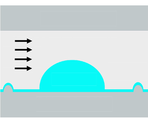
Figure 1(a) shows the model geometry, where we consider a rectangular channel containing a two-dimensional Newtonian droplet surrounded by another immiscible Newtonian fluid. Here,  $W$ is the channel width, $L$ is the channel length, $h(x,t)$ is the droplet height, $\theta _{acl}$ is the apparent advancing contact angle and $\theta _{rcl}$ is the apparent receding contact angle. The horizontal direction is denoted by $x$, the vertical direction by $y$ and time by $t$. We consider a thin droplet such that its height is much smaller than its diameter (maximum width), and we assume it is confined in a long narrow channel such that $W \ll L$. This allows us to invoke the lubrication approximation to simplify the governing equations. A negative horizontal pressure gradient is imposed in the channel to drive flow. Although a two-dimensional droplet is actually a ridge, we refer to it as a droplet in the remainder of this paper for simplicity.
(a) Schematic of model geometry. (b) Enlarged view of a substrate defect.

Surface roughness is incorporated by adding bump-type defects on the substrate. Figure 1(b) shows an enlarged view of a defect, where  $h_d$ is the maximum defect height and $w_d$ is the maximum defect width. In practical applications, substrates can have defects of different sizes and shapes present at random locations. Here, we focus on the limiting case where a Gaussian bump-type defect is present at a distance $x_d$ from each contact line. This reduces the complexity of the problem while allowing us to obtain physical insight into the influence of substrate topography on the droplet dynamics. The substrate topography is described by the function $\eta (x) = h_d \{\exp (-(x - x_{c1})^2/(2 w_d^2)) + \exp (-(x - x_{c2})^2/(2 w_d^2))\}$, where $x_{c1}$ is the centre of the defect on the left and $x_{c2}$ is the centre of the defect on the right.
2.1. Governing equations
Several applications discussed in § 1, such as cross-flow microemulsification (Charcosset et al. Reference Charcosset, Limayem and Fessi2004) and oil recovery (Eckmann et al. Reference Eckmann, Cavanagh and Branger2001), involve long and narrow channels, which corresponds to  $\epsilon = W/L \ll 1$ for our model. Consistent with lubrication theory, the maximum droplet height $h_{max}$ is assumed to be much smaller than its diameter $D$, with $h_{max} \sim W$ and $D \sim L$ at most. In principle, lubrication theory requires the topography slope to be small, but in practice lubrication theory can yield qualitatively accurate predictions for two-phase problems even outside of this regime, as demonstrated by comparison with numerical simulations of the full governing equations (Zhou & Kumar Reference Zhou and Kumar2012).
The vertical and horizontal distances are non-dimensionalized with  $W$ and $L$, respectively. All stresses are scaled with a characteristic capillary pressure $W\sigma /L^2$, where $\sigma$ is the interfacial tension (Schwartz & Eley Reference Schwartz and Eley1998). The horizontal velocity is scaled with a capillary spreading speed $u^* = \epsilon ^3\sigma /3\mu ^d$, where $\mu ^d$ is the droplet viscosity, the vertical velocity is scaled with $\epsilon u^*$ and time is scaled with $L/u^*$.
At leading order, the mass and momentum conservation equations in each phase are
 $$\begin{gather} u^i_{x} + v^i_{y} = 0, \end{gather}$$
 $$\begin{gather}(\mu^i/\mu^d) u^i_{yy} = 3P^i_{x}, \end{gather}$$
 $$\begin{gather}P^i_y + (\rho^i/\rho^d) Bo = 0, \end{gather}$$
where the superscript  $i$ denotes the phase ( $i = d$ for droplet, and $i = s$ for surrounding fluid), $u$ is the horizontal velocity, $v$ is the vertical velocity, $\mu$ is the viscosity, $P$ is the pressure and $\rho$ is the density. Three dimensionless parameters arise here: (i) the Bond number $Bo = \rho ^d g L^2 / \sigma$, where $g$ is the magnitude of the gravitational acceleration, which represents a ratio of gravitational forces to surface-tension forces, (ii) the viscosity ratio $\mu _r = \mu ^s / \mu ^d$ and (iii) the density ratio $\rho _r = \rho ^s / \rho ^d$. In this work, we assume $Bo \ll 1$ to isolate the influence of the imposed pressure gradient on the droplet dynamics.
Motivated by prior work on droplet motion on a solid substrate, we use a precursor-film/disjoining-pressure approach to model contact-line motion (Schwartz Reference Schwartz1998; Schwartz & Eley Reference Schwartz and Eley1998; Espín & Kumar Reference Espín and Kumar2015, Reference Espín and Kumar2017; Charitatos, Pham & Kumar Reference Charitatos, Pham and Kumar2021; Mhatre & Kumar Reference Mhatre and Kumar2024). As opposed to approaches that impose a slip law on the substrate, here, the contact-line position is extracted from the droplet height profile (see § 2.2) and is not an extra variable, which makes the resulting equations less cumbersome to solve (Savva & Kalliadasis Reference Savva and Kalliadasis2011). This approach assumes the presence of a precursor film of thickness  $b$ along the entire substrate (figure 1). The total pressure within the droplet is $P = P^{'} + \varPi$, where $P^{'}$ is the hydrodynamic pressure and $\varPi$ is the disjoining pressure. A two-term disjoining pressure is used
 \begin{equation} \varPi = A \left[\left(\frac{b}{h}\right)^n - \left(\frac{b}{h}\right)^m\right], \end{equation}
where  $A$ is the dimensionless Hamaker constant and $h$ is the droplet thickness. The term with exponent $n$ represents contributions from repulsive intermolecular forces, and the term with exponent $m$ represents contributions from attractive intermolecular forces. We choose $n=3$ and $m=2$, as prior studies show that these values provide qualitatively accurate predictions of contact-line motion at a reasonable computational cost (Espín & Kumar Reference Espín and Kumar2015, Reference Espín and Kumar2017; Charitatos et al. Reference Charitatos, Pham and Kumar2021). It should be noted that our model can be extended to incorporate chemical heterogeneity on the substrate by spatially varying $A$ (Schwartz Reference Schwartz1998; Schwartz & Eley Reference Schwartz and Eley1998; Kalpathy, Francis & Kumar Reference Kalpathy, Francis and Kumar2012).
The two-term disjoining pressure determines an equilibrium contact angle of magnitude  $\theta _{eq}$, which the droplet attains in the absence of an imposed pressure gradient (Schwartz & Eley Reference Schwartz and Eley1998)
 \begin{equation} \theta_{eq} = \sqrt{\frac{2(n-m)A b}{(n-1)(m-1)}}. \end{equation}
Here,  $\theta _{eq}$ is the scaled equilibrium contact angle and is related to the actual laboratory-frame equilibrium contact angle by $\theta _{eq, lab} = \epsilon \theta _{eq}$. All the angles discussed in the remainder of this paper are scaled angles.
The interface between the droplet and the surrounding fluid is described as  $H(x,t) = h(x,t) + \eta (x)$, and we impose the following conditions:
 $$\begin{gather} u^d = u^s, \end{gather}$$
 $$\begin{gather}v^d = v^s, \end{gather}$$
 $$\begin{gather}P^d - P^s ={-}H_{xx}, \end{gather}$$
 $$\begin{gather}u^d_y = \mu_r u^s_y, \end{gather}$$
 $$\begin{gather}h_t + \left( \int_{\eta}^{H} u^d \,{{\rm d} y} \right)_x = 0, \end{gather}$$
where (2.6) and (2.7) are continuity of velocity, (2.8) is the normal stress balance, (2.9) is the tangential stress balance and (2.10) is the kinematic condition. No-slip and no-penetration conditions are imposed at the substrate ( $y = \eta (x)$) and the top boundary ( $y = 1$)
 $$\begin{gather} u^d (y = \eta, t) = 0, \quad u^s (y = 1, t) = 0, \end{gather}$$
 $$\begin{gather}v^d (y = \eta, t) = 0, \quad v^s (y = 1, t) = 0. \end{gather}$$
 An imposed pressure gradient in the channel generates a mean flow rate in the  $x$-direction, and we represent its dimensionless form by $Q_p$. Due to mass conservation, $Q_p$ does not vary along the $x$-direction, and we calculate it by considering a portion of the channel that only contains the precursor film, as it is a steady two-layer flow with a flat interface of height $b$
$b$
 \begin{equation} Q_p = \frac{1}{4} \Delta P \left({-}b^3 + \frac{3b(b-1)}{1+(\mu_r-1)b} + \frac{(b-1)^3}{\mu_r} \right). \end{equation}
Here,  $\Delta P$ denotes the magnitude of the dimensionless imposed pressure gradient. Since the precursor-film thickness is much smaller than the channel width ( $b \ll 1$), the flow rate simplifies to $Q_p = \Delta P / 4\mu _r$, which is used in the flow-rate condition
 \begin{equation} \int_{\eta}^{H} u^d \,{{\rm d} y} + \int_{H}^{1} u^s \,{{\rm d} y} = Q_p. \end{equation}
We find that the qualitative nature of our results does not change if we use (2.13) in the flow-rate condition, and the quantitative difference is approximately  $5$ %– $10\,\%$. We use the simplified flow rate here to eliminate the dependence on $b$.
$b$.
Integrating (2.2) and (2.3) with respect to  $y$ and using conditions (2.6)–(2.14) gives the droplet height evolution equation
 \begin{align} \frac{\partial h}{\partial
t} &= \frac{\partial}{\partial x} \left[ \frac{(H-1)^3h^3
f(H,\mu_r, \eta)}{g(H,\mu_r, \eta)} \left( \frac{\partial
H^3}{\partial x^3} + \frac{\partial \varPi}{\partial
x}\right) \right.\nonumber\\ & \quad + \left. \Delta P
\frac{h^3 (3+H^2(\mu_r-1))-2H(1+(\mu_r-2)\eta + \eta(\mu_r
\eta - 4))}{4 f(H,\mu_r, \eta)} \right],
\end{align}
\begin{align} \frac{\partial h}{\partial
t} &= \frac{\partial}{\partial x} \left[ \frac{(H-1)^3h^3
f(H,\mu_r, \eta)}{g(H,\mu_r, \eta)} \left( \frac{\partial
H^3}{\partial x^3} + \frac{\partial \varPi}{\partial
x}\right) \right.\nonumber\\ & \quad + \left. \Delta P
\frac{h^3 (3+H^2(\mu_r-1))-2H(1+(\mu_r-2)\eta + \eta(\mu_r
\eta - 4))}{4 f(H,\mu_r, \eta)} \right],
\end{align}where
 \begin{gather} f(H,\mu_r,\eta) = 1+H(\mu_r-1)-\mu_r\eta, \end{gather}
 $$\begin{gather} g(H,\mu_r,\eta) = (H-\eta)^4 \mu_r^2 - 2\mu_r(H-1)(H^3-H^2(1+2\eta) \nonumber\\ +\eta({-}2+3\eta-2\eta^2)+H(2-2\eta+3\eta^2)) +(H-1)^4.\end{gather}$$
 We set the length of the computational domain to  $L$, and require the interface between the precursor film and the surrounding fluid to be flat at the left and right ends
 $$\begin{gather} h(x = 0, t) = b, \quad \hfill h_x (x = 0, t) = 0, \end{gather}$$
 $$\begin{gather}h(x=L, t) = b, \quad h_x (x = L, t) = 0. \end{gather}$$
We use a fourth-order polynomial which satisfies (2.18a,b) and (2.19a,b), and specify a dimensionless droplet volume  $v_0$, to define the initial droplet shape. Evolution equation (2.15) is discretized using a fully implicit centred fourth-order finite-difference scheme with 6000–8000 spatial nodes, and the MATLAB built-in solver ode15s is used for time integration. All results were checked to ensure that they are converged with respect to spatial and temporal discretization.
In the simulations presented here, we set  $L =6$ or $L = 9$ to obtain results that are independent of the length of the computational domain. A value of $b=0.001$ is used as it allows us to recover Tanner's spreading law for a two-dimensional droplet (§ 3) while allowing for reasonable computation times. For all calculations with rough surfaces, the precursor-film thickness is much smaller than the defect amplitude ( $b/h_d \sim$ $10^{-2}$– $10^{-1}$), indicating that the bump accounts for surface roughness in a physically realistic manner. Smaller values of $b$ lead to slower droplet spreading and a more computationally stiff problem, but do not change the qualitative behaviour of the results presented here. For many of our results, we use representative values of $v_0=0.2$ and $\theta _{eq} = 10^{\circ }$ (which corresponds to $A=10^5$ using (2.5)), although we also study the effect of changing these parameters. In this paper, the largest value of $\theta _{eq}$ is $16^\circ$, which corresponds to $\tan {\theta _{eq}} \sim 10^{-1}$ and small interfacial slopes, consistent with the lubrication approximation.
2.2. Contact angles and contact lines
For a smooth substrate, we define apparent advancing ( $\theta _{acl}$) and receding ( $\theta _{rcl}$) contact angles (figure 1a) as the largest angles between the substrate and the tangents to the interface between the droplet and the surrounding fluid, on the advancing and receding sides of the droplet. Advancing and receding contact-line locations, $x_{acl}$ and $x_{rcl}$, are defined as the points where the tangents corresponding to the apparent contact angles and the substrate intersect. In the absence of an external pressure gradient $\theta _{acl} = \theta _{rcl}$. If $\theta _{acl} > \theta _{eq}$, the droplet spreads until $\theta _{acl} = \theta _{eq}$, and if $\theta _{acl} < \theta _{eq}$ the droplet retracts until $\theta _{acl} = \theta _{eq}$.
For substrates with topographical defects, a mesoscopic contact angle  $\theta _m$ is defined (Espín & Kumar Reference Espín and Kumar2015; Park & Kumar Reference Park and Kumar2017)
 \begin{equation} \tan(\theta_m) = \frac{h_x}{1+(h_x + \eta_x)h_x}. \end{equation}
The apparent contact angles  $\theta _{acl}$ and $\theta _{rcl}$ are obtained by finding the points on the interface between the droplet and the surrounding fluid where $\theta _m$ is the largest, on the advancing ( $\theta _{ma}$ in figure 2a) and receding ( $\theta _{mr}$ in figure 2b) sides of the droplet, respectively, and then extrapolating the tangents at these points to the substrate. The contact-line positions $x_{acl}$ and $x_{rcl}$ are defined as the points where the tangents corresponding to the apparent contact angles and the substrate intersect.
(a) Contact-line region when the advancing contact line moves over a defect, where  $\eta$ represents the substrate shape, $H$ represents the interface shape, $\theta _{acl}$ is the apparent advancing contact angle and $\theta _{ma}$ is the largest mesoscopic angle on the advancing half of the droplet interface. (b) Contact-line region when the receding contact line moves over a defect, where $\theta _{rcl}$ is the apparent receding contact angle and $\theta _{mr}$ is the largest mesoscopic angle on the receding half of the droplet interface.

3. Droplet dynamics on a smooth substrate
Before considering the influence of substrate topography on the droplet dynamics, we discuss the case of a smooth substrate, which corresponds to  $\eta (x) = 0$. We first consider the case of a droplet spreading on a substrate while surrounded by a stationary fluid ( $\Delta P = 0$). For perfectly wetting droplets ( $\theta _{eq}=0^{\circ }$), our results (figure 1 of supplementary material available at https://doi.org/10.1017/jfm.2024.451) are consistent with Tanner's spreading law for a two-dimensional droplet ( $x_{acl} - x_c \sim t^{1/7}$, where $x_c$ is the droplet centre) (Tanner Reference Tanner1979). This holds for all viscosity ratios we have investigated, with an increase in the surrounding fluid viscosity simply slowing the spreading. For partially wetting droplets, viscosity has a similar effect, as seen in figure 3. The droplet spreads ( $x_{acl}$ increases and $\theta _{rcl}$ decreases) at earlier times, and eventually reaches the same steady shape for all $\mu _r$ since the steady droplet shape is governed by $\theta _{eq}$ (Schwartz & Eley Reference Schwartz and Eley1998). The steady $\theta _{acl}$ ( $\approx 11^{\circ }$) found from numerical simulations is within approximately $1^{\circ }$ of the specified $\theta _{eq} = 10^{\circ }$ from (2.5).
Droplet dynamics on a smooth substrate in a stationary surrounding fluid. (a) Plot of  $x_{acl}$ vs $t$ for different $\mu _r$. (b) Plot of $\theta _{acl}$ vs $t$ for different $\mu _r$. The other parameters are $L=6$, $A = 10^5$ ( $\theta _{eq} = 10^{\circ }$), $b=0.001$ and $v_0 = 0.2$.

To study the influence of a surrounding fluid flow, we first perform a simulation such that the droplet reaches a steady shape in a stationary surrounding fluid to obtain an initial condition. We then introduce a negative horizontal pressure gradient of magnitude  $\Delta P$ within the channel. Figure 4(a) shows the variation of $x_{acl}$ with $t$ for different $\Delta P$. The slope of $x_{acl}$ vs $t$ at any point represents the horizontal velocity of the advancing contact line, and it is seen that this velocity reaches a steady value, which we denote as the terminal sliding velocity, $v_t$. Figure 4(b) shows the steady droplet shapes for different $\Delta P$ values. The droplet is shorter and wider for $\Delta P > 0$ compared with $\Delta P = 0$, and the deformation increases with $\Delta P$. For a constant $\Delta P$, additional calculations we have performed indicate that the droplet takes longer to attain a steady shape as $\mu _r$ increases. The steady shape is relatively independent of $\mu _r$ for $\mu _r \lesssim 1$, but the amount of deformation noticeably increases for sufficiently large $\mu _r$ values.
Droplet dynamics on smooth substrates. (a) Plot of  $x_{acl}$ vs $t$ for different $\Delta P$, with $\mu _r = 0.01$ and $v_0 = 0.2$. (b) Steady droplet shapes for different $\Delta P$ on a smooth substrate. The droplet profiles have been shifted such that their receding contact lines coincide. (c) Plot of $v_t$ vs $\Delta P$, with $\mu _r = 0.01$ and $v_0 = 0.2$. The other parameters are $\mu _r = 0.01$, $v_0 = 0.2$, $L=9$, $A = 10^5$ ( $\theta _{eq} = 10^{\circ }$) and $b=0.001$.

The results from the numerical simulations can be rationalized by using a flat-interface approximation, where we assume a steady pressure-driven two-layer flow with a flat interface such that the bottom layer consists of the droplet liquid and the top layer consists of the surrounding fluid. The physical variables are non-dimensionalized using the characteristic scales discussed in § 2.1, and the dimensionless horizontal liquid velocity at the interface is calculated to be
 \begin{equation} v_H = \frac{3 \Delta P (1-H)H}{2 (1+H(\mu_r - 1))}, \end{equation}
where  $H$ is the dimensionless height of the flat interface.
For a given  $\Delta P$ and $\mu _r$, we perform a numerical simulation for a droplet to calculate $v_t$ and the steady shape it attains, from which we extract the maximum droplet height ( $h_{max}$). We set $H = h_{max}$, calculate $v_H$ using (3.1) and compare it with $v_t$.
Figure 4(c) shows that  $v_t \sim \Delta P$, which is consistent with the flat-interface approximation (3.1). Calculating $v_H$ from (3.1) reveals that the flat-interface approximation overpredicts $v_t$ by a factor of approximately 3.6, likely because the flat-interface approximation does not account for the influence of viscous dissipation and surface-tension forces near the droplet contact line.
Figure 5(a) shows the variation of  $v_t$ with $\mu _r$, where the open blue circles are results from numerical simulations for the droplet, and the dashed red line is from the flat-interface approximation $(v_H)$. The flat-interface approximation overpredicts $v_t$ by nearly an order of magnitude. However, it reproduces the qualitative trend observed from droplet simulations, where $v_t$ is not strongly dependent on $\mu _r$ for $\mu _r < 1$, and decreases with $\mu _r$ for $\mu _r > 1$. This trend can be rationalized by considering (3.1). From (3.1), $v_H \approx (3 H \Delta P /2)$ for $\mu _r \ll 1$, and $v_H \approx (3 \Delta P (1-H) / 2 \mu _r)$ for $\mu _r \gg 1$. Note that, for both $\mu _r \ll 1$ and $\mu _r \gg 1$, the flat-interface approximation predicts that $v_H$, and thus $v_t$, $\sim \Delta P$.
(a) Plot of  $v_t$ vs $\mu _r$, with $\Delta P = 0.04$, $A = 10^5$ ( $\theta _{eq} = 10^{\circ }$) and $v_0 = 0.2$. (b) Plot of $\log (v_t)$ vs $\log (v_0)$, with $\mu _r = 0.01$, $A = 10^5$ ( $\theta _{eq} = 10^{\circ }$) and $\Delta P = 0.04$. (c) Plot of $v_t$ vs $\theta _{eq}$, with $\mu _r = 0.01$, $\Delta P = 0.04$ and $v_0 = 0.2$. The other parameters are $L=9$ and $b=0.001$.

To explore the effects of droplet volume, figure 5(b) shows  $\log (v_t)$ vs $\log (v_0)$, with $v_0$ being the droplet volume, for $\mu _r = 0.01$, where the open blue circles are from numerical simulations for the droplet, and the dashed black line is a linear fit which indicates that $v_t \sim v_0^{0.4}$. Droplet simulations for $\mu _r = 100$ also yield $v_t \sim v_0^{0.4}$. Using the flat-interface approximation (3.1), $v_H \approx (3 H \Delta P /2)$ for $\mu _r \ll 1$, and $v_H \approx (3 \Delta P (1-H) / 2 \mu _r)$ for $\mu _r \gg 1$. This suggests that $v_t \sim h_{max}$ for the droplet, for both $\mu _r \ll 1$ and $\mu _r \gg 1$. From the simulations for both the cases, it is found that $h_{max}$ $\sim v_0 ^ {0.5}$ for a droplet after it attains a steady shape, and thus we obtain $v_t \sim v_0^{0.5}$, which is close to the scaling relation obtained from droplet simulations. (Note that the simulations also show that the steady value of $D = x_{acl} - x_{rcl} \sim v_0^{0.5}$, consistent with mass conservation.)
Figure 5(c) shows  $v_t$ vs $\theta _{eq}$, where the open blue circles are results from numerical simulations for the droplet, and the dashed red line is from the flat-interface approximation $(v_H)$. The flat-interface approximation overpredicts $v_t$, but it reproduces the qualitative trend observed from droplet simulations. This is because $h_{max}$, and consequently $H$, increase with $\theta _{eq}$, and $v_H$ increases monotonically with $H$, as can be seen by analysing (3.1). Although it misses important details, the flat-interface approximation is also useful for understanding the droplet dynamics on rough substrates, as will be shown later.
4. Droplet dynamics on a rough substrate
In this section, we study the influence of substrate topography. To obtain an initial condition for a given set of parameters, we perform a numerical simulation such that the droplet reaches a steady shape on a smooth substrate in a stationary surrounding fluid, then add a Gaussian bump-type defect (discussed in § 2) at each contact line with  $x_d = 0$ (figure 1a) to pin the droplet. We then introduce a negative horizontal pressure gradient of magnitude $\Delta P$ in the channel. For the calculations presented in this section we fix $h_d = 0.02h_{max}$ and $w_d = 2h_d$ to isolate the effects of $\Delta P$. The influence of defect geometry on the droplet dynamics is discussed in § 6.2.
4.1. Pinning–depinning transition
Figures 6(a) and 6(b) show the variation of  $\theta _{acl}$ and $x_{acl}$ with $t$ for $\Delta P = 0.05$ and $\Delta P = 0.07$. For $\Delta P = 0.05$, $x_{acl}$ does not vary with $t$, and $\theta _{acl}$ increases with $t$ to eventually reach a steady value. This behaviour is indicative of droplet pinning. For $\Delta P = 0.07$, $\theta _{acl}$ increases with $t$ and $x_{acl}$ remains constant until $t = 266$. Then, for $t > 266$, $\theta _{acl}$ decreases with $t$ and eventually reaches a steady value, and $x_{acl}$ increases with $t$. This behaviour is indicative of droplet depinning. Overall, these results suggest that there is a critical pressure gradient $\Delta P_{crit}$ above which droplet depinning occurs.
Droplet dynamics on a rough substrate. (a) Plot of  $\theta _{acl}$ vs $t$. (b) Plot of $x_{acl}$ vs $t$. The kinks in $x_{acl}$ at $t = 266$ indicate that the contact line rapidly depins from the defect at that time and shifts to the right. The smaller kink to the left of the larger kink arises while numerically resolving $x_{acl}$ from droplet profiles. The other parameters are $L=9$, $\mu _r = 0.01$, $A = 10^5$ ( $\theta _{eq} = 10^{\circ }$), $b=0.001$, $v_0 = 0.2$, $h_d = 0.02h_{max}$ and $w_d = 2h_d$.

Figure 7(a) shows the variation of the steady  $\theta _{acl}$ value with $\Delta P$, and it is seen that $\theta _{acl}$ increases with $\Delta P$ for $\Delta P < 0.063$. For $\Delta P < 0.063$, it is found that $x_{acl}$ remains equal to its initial value, similar to what is seen for $\Delta P = 0.05$ (blue line in figure 6b). As $\Delta P$ increases from zero, the droplet remains pinned but becomes increasingly deformed, as shown in figure 7(b).
(a) Steady value of  $\theta _{acl}$ vs $\Delta P$. (b) Steady droplet profiles for different $\Delta P$. (c) Droplet profiles at different $t$ for $\Delta P = 0.07$. The solid black lines show substrate topography and the other lines show droplet profiles. All other parameters are the same as in figure 6.

At  $\Delta P = 0.063$, a significant decrease in $\theta _{acl}$ is observed, indicating droplet depinning, and for $\Delta P > 0.063$, there is a slight increase in $\theta _{acl}$ with $\Delta P$. Furthermore, for $\Delta P > 0.063$, the behaviour of $x_{acl}$ as a function of $t$ is qualitatively similar to that for $\Delta P = 0.07$ (red line in figure 6b), where $x_{acl}$ remains equal to the initial value for a period of time and then gradually increases with $t$. Thus, after the droplet depins it slides on the substrate with a steady shape, as shown in figure 7(c) (see supplementary material for videos of droplet pinning and depinning).
4.2. Droplet pinning mechanism
As discussed in § 1, the pinning–depinning transition has been rationalized in prior work using simple force-balance models (Fan et al. Reference Fan, Wilson and Kapur2011; Lu et al. Reference Lu, Xu, Xie, Wang, Sun and Yang2019). We apply those ideas here to see how well they describe our results. In those models, the drag force acting on the droplet due to the surrounding fluid flow drives depinning, and the surface-tension force acting along the droplet contact line resists depinning. The total drag force acting on the droplet is predominantly composed of skin drag and the pressure drag is negligible. Also, the total drag force is nearly equal to the shear force due to the droplet being thin (figure 2 of supplementary material). We note that pressure drag is expected to become significant for droplets not well described by the lubrication approximation. The balance between the shear force and the surface-tension force can be represented in a dimensionless form as  $(D^2/h_{max})(\cos {\theta _{rcl}} - \cos {\theta _{acl}}) \sim \int _{s} \boldsymbol {n}\boldsymbol {\cdot }\boldsymbol {T}\boldsymbol {\cdot }\boldsymbol {t} \,{\rm d}s$ (see Appendix A). Here, $D = x_{acl} - x_{rcl}$ is the droplet width, $h_{max}$ is the maximum droplet height, $\boldsymbol {n}$ is the unit normal vector at the interface between the droplet and the surrounding fluid that points into the surrounding fluid, $\boldsymbol {T}$ is the droplet stress tensor, $\boldsymbol {t}$ is the unit tangent vector at the interface and $s$ is the interface arclength coordinate such that $s = 0$ at the receding contact line and $s = 1$ at the advancing contact line.
We extract the values of  $D$,
$D$,  $h_{max}$, $\theta _{acl}$, $\theta _{rcl}$, $\boldsymbol {n}$, $\boldsymbol {T}$ and $\boldsymbol {t}$ from the steady droplet shapes in numerical simulations to calculate the terms in the force balance. Figure 8(a) shows these terms for different $\Delta P < \Delta P_{crit}$, with the open red circles presenting the simulation results. As can be seen, there is indeed a linear relationship, consistent with the force-balance model. It should be noted that inertial forces may become important for larger droplets or larger $\Delta P$ values (Mortazavi & Jung Reference Mortazavi and Jung2023), but they are neglected in this work.
(a) Terms in the force-balance model for pinned droplets at different  $\Delta P$ values. The open red circles are results from numerical simulations and the straight blue line has a slope of unity. (b) Enlarged view of the pinned advancing contact line for $\Delta P = 0.03$, where the blue line shows the droplet and the red line shows the defect. (c) Enlarged view of the pinned receding contact line for $\Delta P = 0.03$, where the blue line shows the droplet and the red line shows the defect. The other parameters are $L=9$, $\mu _r = 0.01$, $A = 10^5$ ( $\theta _{eq} = 10^{\circ }$), $b=0.001$, $v_0 = 0.2$, $h_d = 0.02h_{max}$ and $w_d = 2h_d$.

Next, we discuss the pinning locations of the two contact lines. It can be seen from figure 8(b,c) that the following geometric relations hold at the pinned advancing and receding contact lines:
 $$\begin{gather} \theta_{acl} = \theta_{ma} + \gamma_{a}, \end{gather}$$
 $$\begin{gather}\theta_{rcl} = \theta_{mr} - \gamma_{r}, \end{gather}$$
where  $\gamma _a$ is the magnitude of the slope at the point on the defect on the right that coincides with $x_{acl}$, and $\gamma _r$ is the magnitude of the slope at the point on the defect on the left that coincides with $x_{rcl}$. Our calculations show that, for all the cases of a pinned droplet, $\theta _{ma} \approx \theta _{mr} \approx \theta _{eq}$, so the values of $\theta _{rcl}$ and $\theta _{acl}$ depend primarily on $\gamma _r$ and $\gamma _a$, respectively.
For all the cases where the droplet is pinned, it is found that  $x_{rcl}$ and $x_{acl}$ coincide with the points on the defects where there is a maximum negative slope, whose magnitude we denote as $\gamma _{max}$. Using (4.1) and (4.2), it can be seen that, as a consequence of these pinning locations, $\theta _{rcl} \approx \theta _{eq} - \gamma _{max}$ is minimized, and $\theta _{acl} \approx \theta _{eq} + \gamma _{max}$ is maximized, which maximizes the surface-tension term in the force-balance model $(D^2/h_{max})(\cos {\theta _{rcl}} - \cos {\theta _{acl}})$. These findings are consistent with predictions from a lubrication-theory-based model for a droplet sliding down an inclined substrate with a single Gaussian-shaped bump, where the advancing contact line pins at the point on the bump that has the maximum negative slope, as it maximizes the surface-tension force (Park & Kumar Reference Park and Kumar2017). The present work shows that similar behaviour occurs even in more complicated situations, where the geometry and driving force for flow are different, and the dynamics of both phases are accounted for.
The pinning–depinning transition can also be understood through an analysis of the pressure gradients in the droplet (Espín & Kumar Reference Espín and Kumar2015; Charitatos et al. Reference Charitatos, Pham and Kumar2021). Figure 9 shows the variation of the pressure in a pinned droplet with  $x$ for two $\Delta P$ values. The total pressure includes contributions from the capillary pressure and the disjoining pressure, and figure 9 shows the former quantity as well. For each case, the capillary pressure has a negative gradient and drives flow from the droplet interior toward the advancing contact line (located at $x = 5.56$), which promotes depinning. However, the disjoining pressure increases closer to the contact line, and causes the total pressure gradient within the droplet to become positive, which drives flow from the advancing contact line toward the droplet interior. Near the receding contact line, the total pressure gradient within the droplet is negative (figure 3 of supplementary material), which drives flow from the receding contact line toward the droplet interior. The flows near the two contact lines oppose each other and result in a pinned droplet.
Droplet pressure vs  $x$ for pinned droplets. The dashed blue line shows the contribution from the capillary pressure and the solid red line shows the total pressure (capillary and disjoining). All the other parameters are the same as in figure 8.

As  $\Delta P$ increases, the pinned droplet becomes increasingly deformed (see figure 7b), which increases the droplet thickness near the advancing contact line and decreases the disjoining pressure there. As a result, the total pressure gradient near the advancing contact line decreases, as shown in figure 9. At $\Delta P_{crit}$, the total pressure gradient near the advancing contact line becomes negative, and the total pressure gradient near the receding contact line remains negative. This results in a net negative pressure gradient within the droplet, which causes the two contact lines to depin simultaneously, and the droplet slides to the right.
4.3. Droplet depinning time
The time it takes the droplet to depin when  $\Delta P > \Delta P_{crit}$ is of both fundamental and practical interest. The droplet depinning time, $t_{depinning}$, is calculated as the time at which the receding contact-line position, $x_{rcl}$, crosses the defect on the right. A scaling relation can be obtained for $t_{depinning}$ by dividing the droplet width, $D$, with the droplet velocity (3.1) obtained from the flat-interface approximation (§ 3). For $\mu _r \ll 1$, this yields $t_{depinning} \sim D / {\Delta P h_{max}}$.
Figure 10 shows  $\log {t_{depinning}}$ vs $\log {D / ({\Delta P h_{max}})}$, where the open blue circles are results from numerical simulations and the dashed black line has a slope of $1$. The intercept for the dashed black line is chosen such that it overlaps with the simulation result at $\log {D / (\Delta P h_{max})} = 4.1814$. Fitting a straight line to the numerical calculations yields a slope of $1.423$. Thus, the scaling law derived above predicts a faster depinning time ( ${\sim D / (\Delta P h_{max})}$) than what is observed from numerical simulations ( ${\sim (D/(\Delta P h_{max}))^{1.423}}$). This is expected based on the results in § 3, as the flat-interface approximation does not account for viscous dissipation and surface-tension forces near the contact lines, which slow down droplet motion.
Plot of  $\log {t_{depinning}}$ vs $\log {D/(\Delta P h_{max})}$, where the open blue circles show results from numerical simulations, and the dashed black line shows a slope of $1$. The other parameters are $L=9$, $\mu _r = 0.01$, $A = 10^5$ ( $\theta _{eq} = 10^{\circ }$), $b=0.001$, $v_0 = 0.2$, $h_d = 0.02h_{max}$ and $w_d = 2h_d$.

5. Influence of droplet and surrounding fluid properties on the critical pressure gradient
5.1. Influence of viscosity ratio
Figure 11(a) shows  $\Delta P_{crit}$ vs $\mu _r$. For $\mu _r < 1$, $\Delta P_{crit}$ decreases slightly with $\mu _r$, and this result is qualitatively consistent with the experimental observations of Fan et al. (Reference Fan, Wilson and Kapur2011) where, as the viscosity of the glycerol–water droplet increases (by increasing the glycerol concentration), a larger critical flow rate of the surrounding air is required to depin it on a treated glass surface. For $\mu _r > 1$, $\Delta P_{crit}$ decreases with $\mu _r$ to reach a minimum value at $\mu _r \approx 10$, and then increases with $\mu _r$. These results can be rationalized by examining the shear force acting on the droplet. Our calculations show that the surface-tension force does not vary significantly with $\mu _r$ ( $\approx 6\,\%$), so we do not consider it here.
(a) Plot of  $\Delta P_{crit}$ vs $\mu _r$. (b) Shear force vs $\mu _r$ for $\Delta P = 0.03$. (c) Plot of $\partial u^s / \partial y$ at the maximum height of pinned droplet vs $\mu _r$ for $\Delta P = 0.03$. The other parameters are $L=9$, $\mu _r = 0.01$, $A = 10^5$ ( $\theta _{eq} = 10^{\circ }$), $b=0.001$, $v_0 = 0.2$, $h_d = 0.02h_{max}$ and $w_d = 2h_d$.

Figure 11(b) shows shear force vs  $\mu _r$ for a fixed $\Delta P < \Delta P_{crit}$. Using lubrication theory, the shear force $\int _{s} \boldsymbol {n}\boldsymbol {\cdot }\boldsymbol {T}\boldsymbol {\cdot }\boldsymbol {t} \,{\rm d}s$ simplifies to $\int _{s} \mu _r \partial u^s / \partial y \,{\rm d}s$, where $\partial u^s /\partial y$ is the horizontal velocity gradient with respect to $y$ in the surrounding fluid at the interface. For a constant $\Delta P$, as $\mu _r$ increases, the surrounding fluid becomes more viscous and exerts a larger shear force on the droplet. However, for $\mu _r \gg 1$, the surrounding fluid becomes so viscous that the net flow rate along the $x$-direction decreases. Consequently, $\partial u^s / \partial y$ decreases with $\mu _r$, as exemplified in figure 11(c), where $\partial u^s / \partial y$ at the maximum height of the pinned droplet is shown. As a result, the shear force decreases with $\mu _r$ for $\mu _r \gg 1$, and the droplet experiences a maximum shear force, and consequently a minimum $\Delta P_{crit}$ for $\mu _r \approx 10$. This observation is potentially important for applications such as cross-flow microemulsification and oil recovery, where the viscosity of the surrounding fluid could be tuned to minimize $\Delta P_{crit}$.
5.2. Influence of droplet volume
Figure 12(a) shows  $\Delta P_{crit}$ vs $v_0$ for two different values of $\mu _r < 1$ (droplet more viscous than the surrounding fluid). It is seen that $\Delta P_{crit}$ decreases with $v_0$ for each case, and a larger $\Delta P_{crit}$ is required for a smaller $\mu _r$. This result is qualitatively consistent with the experimental findings of Fan et al., where a lower critical flow rate of surrounding air is required to depin a larger glycerol–water droplet on a treated glass surface, and a larger flow rate is required to depin a more viscous droplet of the same volume (Fan et al. Reference Fan, Wilson and Kapur2011). For $\mu _r > 1$, $\Delta P_{crit}$ decreases with $v_0$ as well (figure 4 of supplementary material).
(a) Plot of  $\Delta P_{crit}$ vs $v_0$ for $\mu _r = 0.001$ and $\mu _r = 0.9$. (b) Plot of $\log {\Delta P_{crit}}$ vs $\log {v_0}$ for $\mu _r = 0.001$, where the open blue circles show results from droplet simulations, and the dashed black line shows a linear fit with a slope of $-0.5$. The other parameters are $L=9$, $A = 10^5$ ( $\theta _{eq} = 10^{\circ }$), $b=0.001$, $h_d = 0.02h_{max}$ and $w_d = 2h_d$.

These results can be understood in terms of the force-balance model discussed in § 4.2. An analytical expression is obtained for the shear force acting on the droplet using the flat-interface approximation (see § 3), where the shear stress acting on a flat interface of height  $H$ is multiplied by the length of the horizontal domain $L$
$L$
 \begin{equation} F_s^{flat} = 3\Delta P L \left( H - \frac{1+H^2 (\mu_r - 1)}{2(1+H(\mu_r - 1))} \right). \end{equation}
 Using (5.1) to calculate the shear force by setting  $H = h_{max}$ obtained from the steady droplet profiles, and assuming $L \sim D$, the dimensionless force balance at the point of depinning can be expressed as $3\Delta P_{crit} (h_{max}-1)/2 \sim {(}D/h_{max}(\cos {\theta _{rcl}} - \cos {\theta _{acl}})$ for $\mu _r \ll 1$, and $3\Delta P_{crit} h_{max}/2 \sim (D/h_{max})(\cos {\theta _{rcl}} - \cos {\theta _{acl}})$ for $\mu _r \gg 1$. As discussed in § 3, both $D$ and $h_{max}$ $\sim v_0^{0.5}$. Thus, $\Delta P_{crit} \sim v_0^{-0.5}$ for both $\mu _r \ll 1$ and $\mu _r \gg 1$. Figure 12(b) shows $\log {\Delta P_{crit}}$ vs $\log {v_0}$ for $\mu _r = 0.001$, where the open blue circles are results from numerical simulations and the dashed black line shows a slope of $-0.5$. The close agreement indicates that the flat-interface approximation accurately captures the influence of $v_0$ on $\Delta P_{crit}$. Results from numerical simulations for $\mu _r = 100$ follow the scaling relation as well (figure 4 of supplementary material).
6. Influence of substrate properties on droplet depinning
6.1. Influence of substrate wettability
Figure 13(a) shows  $\Delta P_{crit}$ vs $\theta _{eq}$ for $\mu _r = 0.01$, and it is seen that $\Delta P_{crit}$ increases with $\theta _{eq}$. This result is qualitatively consistent with the experimental findings of Madani & Amirfazli (Reference Madani and Amirfazli2014), where a lower surrounding water flow rate is required to depin an oil droplet ( $\mu _r < 1$) on a more wettable substrate.
(a) Plot of  $\Delta P_{crit}$ vs $\theta _{eq}$. (b) Plot of $(D^2/h_{max}) (\cos {\theta _{rcl}} - \cos {\theta _{acl}})$ vs $\theta _{eq}$ for $\Delta P = 0.03$. The other parameters are $L=9$, $\mu _r = 0.01$, $v_0 = 0.2$, $b=0.001$, $h_d = 0.02h_{max}$ and $w_d = 2h_d$.

These results can be understood by examining the surface-tension term in the force-balance model,  $(D^2/h_{max}) (\cos {\theta _{rcl}} - \cos {\theta _{acl}})$ (see § 4.2), which increases with $\theta _{eq}$ as shown in figure 13(b). The shear force acting on the droplet is not considered as it does not vary significantly with $\theta _{eq}$ ( $\approx 7\,\%$). This can be understood from the flat-interface approximation. According to (5.1), the shear force depends on $h_{max}$, which does not vary significantly with $\theta _{eq}$ ( $\approx 8\,\%$).
As  $\theta _{eq}$ increases, $\theta _{rcl} \approx \theta _{eq} - \gamma _{max}$ increases, which tends to decrease the surface-tension force. Additionally, $\theta _{acl} \approx \theta _{eq} + \gamma _{max}$ increases, which tends to increase the surface-tension force. Overall, a net increase is observed in the surface-tension force (figure 13b), and a larger $\Delta P_{crit}$ is required for droplet depinning on a less wettable substrate.
6.2. Influence of defect geometry
The defect shape is governed by its maximum height  $h_d$ and maximum width $w_d$ (see § 2). It can be seen from figure 1(b) that the maximum slope along the defect $\gamma _{max}$ increases with $h_d$ (constant $w_d$), and decreases with $w_d$ (constant $h_d$). As will be discussed below, $\Delta P_{crit}$ depends only on $\gamma _{max}$, and increasing $h_d$ has the same qualitative effect on the droplet dynamics as decreasing $w_d$. Here, we vary $h_d$ while keeping $w_d$ constant.
Figure 14(a) shows  $\Delta P_{crit}$ vs the ratio of $h_d$ to the initial maximum droplet height, and it is seen that $\Delta P_{crit}$ increases with $h_d$. This result can be understood by examining the surface-tension force acting along the contact line. As discussed in § 6.1, the shear force acting on the droplet for a fixed $\Delta P$ depends on $h_{max}$, which does not vary significantly with $h_d$ ( ${\approx }4\,\%$), and $\mu _r$, which does not vary with $h_d$. As a consequence, the shear force does not vary significantly with $h_d$ ( ${\approx }6\,\%$).
(a) Plot of  $\Delta P_{crit}$ vs $h_d$. (b) Plot of $(D^2/h_{max})(\cos {\theta _{rcl}} - \cos {\theta _{acl}})$ vs $h_d$ for $\Delta P = 0.015$. The other parameters are $L=9$, $\mu _r = 0.01$, $b=0.001$, $A = 10^5$ ( $\theta _{eq} = 10^{\circ }$), $v_0 = 0.2$ and $w_d = 0.008$.

As discussed in § 4.2,  $\theta _{acl} \approx \theta _{eq} + \gamma _{max}$ and $\theta _{rcl} \approx \theta _{eq} - \gamma _{max}$. It can be seen that for a fixed $\theta _{eq}$, as $h_d$, and consequently $\gamma _{max}$, increases, $\theta _{acl}$ increases and $\theta _{rcl}$ decreases. As a result, the surface-tension term in the force-balance model $(D^2/h_{max})(\cos {\theta _{rcl}} - \cos {\theta _{acl}})$ increases with $h_d$, as shown in figure 14(b). Thus, a larger $\Delta P_{crit}$ is required for droplet depinning if taller defects are present on the substrate. Similarly, a larger $\Delta P_{crit}$ is required for narrower defects (figure 5 of supplementary material).
We also find that when the ratio of the defect height to the initial maximum droplet height is greater than  $0.025$ (see dashed line in figure 14a), smaller residual droplets are formed behind and in front of the defect on the right, after the original droplet depins. (The value of 0.025 is specific to the parameters used in the calculations.) We discuss this phenomenon in the next section.
7. Residual droplet formation
7.1. Geometric mechanism
Figure 15 shows droplet profiles as time progresses after the droplet depins, and it is seen that a residual droplet is formed behind the defect on the right as the droplet slides over it. This happens when  $\theta _{rcl} < \gamma _{max}$ as the receding contact line approaches the defect. The disjoining pressure above the defect increases due to droplet thinning, which drives flow away from this region and a smaller residual droplet is pinched off behind the defect. However, if $\theta _{rcl} > \gamma _{max}$, the droplet slides over the defect without leaving behind a residual droplet. It should be noted that $\theta _{rcl}$ is obtained as an output from our calculations (see § 2.2) and generally depends on the viscosity ratio, droplet volume, substrate wettability and defect geometry. These findings are consistent with a prior lubrication-theory-based model for a droplet sliding down an inclined substrate with a single Gaussian-shaped bump, where a residual droplet is formed behind the bump, if $\theta _{rcl} < \gamma _{max}$ as the receding contact line approaches the bump (Park & Kumar Reference Park and Kumar2017).
Droplet profiles at (a)  $t = 500$, (b) $t = 520$ and (c) $t = 540$. Enlarged view of the contact line at (d) $t = 500,$ (e) $t = 520$ and (f) $t = 540$. The solid black lines show substrate topography and the blue lines show droplet profiles. The parameters are $L=9$, $A = 10^5$ ( $\theta _{eq} = 10^{\circ }$), $v_0 = 0.2$, $b=0.001$, $\Delta P = 0.1$, $h_d = 0.02h_{max}$ and $w_d = 2h_d$.

It is also found that an additional residual droplet forms in front of the defect at later times if  $\theta _{rcl} < \gamma _{max}$. Figure 16 shows droplet profiles as time progresses after the formation of the residual droplet behind the defect. As seen in figure 15, the receding contact line remains in the vicinity of the defect during the pinch-off of the residual droplet behind the defect, while the advancing contact line slides to the right. As a result, the droplet elongates and attains a slender concave upward shape on its receding side to the right of the defect as shown in figure 16(a,e). Consequently, the disjoining pressure in this region increases, which drives flow away from the thinnest point of the interface, and a smaller residual droplet is pinched off in front of the defect (figures 16b–d and 16f–h). These findings are also consistent with the prior work discussed above on droplets sliding down an inclined substrate (Park & Kumar Reference Park and Kumar2017), indicating that the condition for residual droplet formation ( $\theta _{rcl} < \gamma _{max}$) holds more generally. Indeed, one would expect this criterion to hold for a broad range of geometries and flows as long as the topography amplitude is much smaller than the length scales characterizing the overall flow. We note that increasing the droplet volume increases the value of $\theta _{rcl}$ when the receding contact line encounters the defect, eventually leading to $\theta _{rcl} > \gamma _{max}$ and suppression of residual droplet formation.
Droplet profiles at (a)  $t = 560$, (b) $t = 580$, (c) $t = 600$ and (d) $t = 620$. Enlarged view of the contact line at (e) $t=560$, (f) $t=580$, (g) $t=600$ and (h) $t=620$. The solid black lines show substrate topography and the blue lines show droplet profiles. The parameters are the same as in figure 15.

The formation of residual droplets has important implications for practical applications. Our results indicate that the presence of topographical defects on the substrate may make it difficult to recover the entire volume of the droplet in applications such as surface cleaning and oil recovery. However, for applications such as microemulsification, our results suggest that the size of the dispersed-phase droplets could be controlled by designing defects to break-up larger droplets into smaller ones.
7.2. Influence of pressure gradient on residual droplet volume
We now consider the influence of  $\Delta P$ on the volume of the residual droplets formed at the defect. The volume of a residual droplet is calculated as $\int _{x_l}^{x_r} h \, \mathrm {d}\kern0.06em x$, where $x_l$ and $x_r$ are the left and right end points of the residual droplet. These values are calculated such that $h>b$
$h>b$  $\forall$ $x_l < x < x_r$ in the region where the residual droplet is present. Figure 17(a) shows residual droplet volume vs $\Delta P$, where the open blue circles are for droplets formed behind the defect, and the open red triangles are for droplets formed in front of the defect. It can be seen that the volume of the droplet formed behind the defect decreases with $\Delta P$. This result can be rationalized by examining the droplet profiles when the receding contact line approaches the defect. Figure 17(b) shows these droplet profiles for different $\Delta P$ values. For each case, the receding contact line slows down as it approaches the defect. As $\Delta P$ increases, the depinned advancing contact line slides faster, leading to a more elongated droplet shape (figure 17b). This results in a larger portion of the droplet being trapped behind the defect just before the residual droplet is pinched off. Thus, a larger residual droplet is formed behind the defect for a larger $\Delta P$ value.
(a) Residual droplet volume vs  $\Delta P$. (b) Droplet profiles at $t = 300$ for different $\Delta P$ values. The solid black line shows substrate topography and the other lines show droplet profiles. The parameters are $L=9$, $A = 10^5$ ( $\theta _{eq} = 10^{\circ }$), $v_0 = 0.2$, $b=0.001$, $\Delta P = 0.1$, $h_d = 0.02h_{max}$ and $w_d = 2h_d$.

Figure 17(a) also shows that the volume of the residual droplet in front of the defect decreases with  $\Delta P$. This can be rationalized by noting that because the receding contact line slides faster after depinning from the defect for larger $\Delta P$ values, there is a shorter time for droplet pinch-off and a smaller residual droplet is formed in front of the defect.
8. Conclusions
We have developed a lubrication-theory-based model to study droplet depinning on rough substrates due to the flow of a surrounding fluid caused by an imposed pressure gradient. In contrast to commonly used force-balance models (Fan et al. Reference Fan, Wilson and Kapur2011; Madani & Amirfazli Reference Madani and Amirfazli2014; Lu et al. Reference Lu, Xu, Xie, Wang, Sun and Yang2019), our model allows for the calculation of steady and transient droplet shapes. In addition, we explicitly account for surface roughness by considering the presence of topographical defects, an important feature not considered in prior computational studies (Li & Pozrikidis Reference Li and Pozrikidis1996; Dimitrakopoulos & Higdon Reference Dimitrakopoulos and Higdon1998; Schleizer & Bonnecaze Reference Schleizer and Bonnecaze1999; Dimitrakopoulos & Higdon Reference Dimitrakopoulos and Higdon2001; Ding & Spelt Reference Ding and Spelt2008; Ding et al. Reference Ding, Gilani and Spelt2010). Another significant difference from prior work is that our model requires specification of only an equilibrium contact angle via a disjoining-pressure function, with advancing and receding contact angle values being outputs of (rather than inputs to) our calculations that are determined by surface topography. Simple analytical models are able to account for many of the features observed in the numerical simulations. A key advantage of the lubrication-theory-based model we have developed is that it can readily be extended to study more complicated situations involving chemical heterogeneity (via a spatially varying disjoining pressure Schwartz Reference Schwartz1998; Schwartz & Eley Reference Schwartz and Eley1998) and three-dimensional effects.
Below a critical value of the pressure gradient,  $\Delta P_{crit}$, the advancing and the receding contact lines of the droplet remain pinned at the defects. Above $\Delta P_{crit}$, the shear force acting on the droplet due to the flow of the surrounding fluid exceeds the surface-tension force acting along the contact line, leading to droplet depinning. The pinning–depinning transition can also be understood in terms of a balance between capillary-pressure gradients and disjoining-pressure gradients. Our simulations reveal that the receding and advancing contact lines always pin at the points on the defects that have the maximum negative slope because this maximizes the surface-tension force acting on the droplet. This is a potentially important finding for applications such as inkjet printing and spray coating, where substrate topography could be designed to pin droplets at specific locations to obtain desired patterns.
As the viscosity of the surrounding fluid increases,  $\Delta P_{crit}$ reaches a minimum before increasing due to a reduction in the shear force acting on the droplet. The presence of this minimum could be exploited to make processes such as oil recovery and cross-flow microemulsification more efficient. Consistent with experimental observations (Fan et al. Reference Fan, Wilson and Kapur2011), our model predicts that larger droplet volumes require a lower $\Delta P_{crit}$, again due to the way the shear force behaves. Less wettable substrates increase the values of $\Delta P_{crit}$ due to the change in surface-tension forces, which are influenced both by the equilibrium contact angle and the maximum slope of the substrate topography, $\gamma _{max}$. This behaviour is also consistent with experimental observations (Madani & Amirfazli Reference Madani and Amirfazli2014). Finally, it is also found that residual droplets may be formed behind and in front of the defect after the droplet depins if $\gamma _{max} > \theta _{rcl}$, which has implications for the efficiency of applications such as oil recovery, surface cleaning and microemulsification.
Although we have considered Gaussian-shaped defects, we expect that our findings will generalize to other defect shapes for situations consistent with the lubrication approximation. Our results also serve as motivation for numerical simulations that relax the lubrication approximation, which are needed to address situations such as (i) defects with vertical sides (e.g. cylindrical and rectangular posts Saal et al. Reference Saal, Straub, Butt and Berger2022) or (ii) droplet–fluid interfaces that become vertical due to sufficiently large contact angles or forces that produce ‘lift-off’ of the droplet from the substrate (Madani & Amirfazli Reference Madani and Amirfazli2014). We expect that some of our findings will generalize to three-dimensional defects as well, as long as the lateral length scale of the defects is sufficiently large compared with the other length scales characterizing the flow geometry. Three-dimensional effects can be addressed within the lubrication approximation, and our work motivates and can be used to help validate such calculations.
Supplementary material and movies
Supplementary material and movies are available at https://doi.org/10.1017/jfm.2024.451.
Acknowledgements
We thank C. Larsson for helpful discussions.
Funding
This material is based upon work supported by the National Science Foundation under grant no. CBET-1935968.
Declaration of interests
The authors report no conflict of interest.
Appendix A
In this section, we derive the expression for the force balance used in § 4.2. We assume that the droplet has a dimensional width  $L_z'$ along the $z$-direction (not shown in figure 1a). The dimensional shear force can be estimated as ${F_s}' \sim {L_z}' \int _{s} \boldsymbol {n}\boldsymbol {\cdot }\boldsymbol {T'}\boldsymbol {\cdot }\boldsymbol {t} \,{\rm d}s'$, where the primes represent dimensional quantities.
The dimensional surface-tension force is estimated by assuming a circular contact line of dimensional diameter  $D'$, such that the contact angle in the entire advancing half is $\theta _{acl}$, and the contact angle in the entire receding half is $\theta _{rcl}$ (Fan et al. Reference Fan, Wilson and Kapur2011)
 $$\begin{gather} F_{cl}' = D' \int_{0}^{{\rm \pi}/2} \sigma \cos{\theta_{acl}} \cos{\alpha} \,{\rm d}\alpha + D' \int_{{\rm \pi}/2}^{\rm \pi} \sigma \cos{\theta_{rcl}} \cos{\alpha} \,{\rm d}\alpha, \end{gather}$$
 $$\begin{gather}F_{cl}' = D' \sigma (\cos{\theta_{rcl}} - \cos{\theta_{acl}}), \end{gather}$$
where  $\alpha \in [0,{\rm \pi} ]$ (due to symmetry) denotes the angular position along the contact line such that $\alpha \in [0,{\rm \pi} /2]$ spans the advancing half of the droplet, and $\alpha \in [{\rm \pi} /2,{\rm \pi} ]$ spans the receding half of the droplet. The dimensional force balance is represented as
 \begin{equation} (D'\sigma)(\cos{\theta_{rcl}} - \cos{\theta_{acl}}) \sim L_z' \int_{s} \boldsymbol{n}\boldsymbol{\cdot}\boldsymbol{T'}\boldsymbol{\cdot}\boldsymbol{t} \,{\rm d}s' . \end{equation}
 We non-dimensionalize the stresses using a capillary pressure  $\sigma W' / L'^2$, and assume $W' \sim h_{max}'$ and $L'\sim D'$, where primes have been used on $W$ and $L$ for notational consistency. This yields
 \begin{equation} (D^2/ h_{max}) (L'^2 / W' L_z')(\cos{\theta_{rcl}} - \cos{\theta_{acl}}) \sim \int_{s} \boldsymbol{n}\boldsymbol{\cdot}\boldsymbol{T}\boldsymbol{\cdot}\boldsymbol{t} \,{\rm d}s , \end{equation}
where  $D = D'/L'$ is the dimensionless droplet diameter, $h_{max} = h_{max}'/W'$ is the dimensionless maximum droplet height and $\boldsymbol {T}$ is the dimensionless droplet stress tensor. Assuming that $L'^2/(W'L_z') \sim 1$, which implies that $L_z' \sim L'/\epsilon$, where $\epsilon = W'/L'$, yields the dimensionless force balance
 \begin{equation} (D^2/ h_{max})(\cos{\theta_{rcl}} - \cos{\theta_{acl}}) \sim \int_{s} \boldsymbol{n}\boldsymbol{\cdot}\boldsymbol{T}\boldsymbol{\cdot}\boldsymbol{t} \,{\rm d}s . \end{equation}


 Open access

