


1. Introduction
Aerofoil noise is one of the major noise components in an aircraft, even more so since the introduction of the high bypass-ratio engine (Lockard & Lilley Reference Lockard and Lilley2004). Thus, aerofoil trailing-edge noise reduction has attracted significant research efforts. Moreover, in recent years, the exponential growth of the wind-energy sector has seen an increasing demand to develop aerodynamically quieter aerofoils for achieving optimal efficiency with high tip speeds (Resor et al. Reference Resor, Maniaci, Berg and Richards2014). Brooks, Pope & Marcolini (Reference Brooks, Pope and Marcolini1989) defined trailing-edge noise as the noise scattered by the interaction of the turbulent boundary layer with the trailing edge of the immersed object. In his seminal work on trailing-edge noise, Amiet (Reference Amiet1976) developed an analytical solution for the trailing-edge noise based on the unsteady pressure fluctuation on the surface of the immersed object (referred to as wall-pressure fluctuation hereafter) and the spanwise coherence length of the turbulent boundary layer at the trailing edge. Thus, in theory, modifications to the boundary-layer characteristics to reduce the wall-pressure fluctuation and the spanwise coherence length can directly lead to the attenuation of trailing-edge noise. However, the prediction of the wall-pressure field within a turbulent boundary layer is complicated as it requires a detailed space–time history of the turbulence (Brooks et al. Reference Brooks, Pope and Marcolini1989), and hence, finding an effective mitigation strategy for trailing-edge noise is often not straightforward.
Several promising techniques for reducing the trailing-edge noise on flat plates and aerofoils have already been studied and established in the literature. These include active noise-control strategies which modify the turbulent boundary layer with external energy input, such as boundary-layer injection (Leitch, Saunders & Ng Reference Leitch, Saunders and Ng2000; Szke, Fiscaletti & Azarpeyvand Reference Szke, Fiscaletti and Azarpeyvand2018) and suction (Wolf et al. Reference Wolf, Lutz, Würz, Krämer, Stalnov and Seifert2015; Szke, Fiscaletti & Azarpeyvand Reference Szke, Fiscaletti and Azarpeyvand2020). The authors of these studies observed a maximum noise reduction of slightly lower than 10 dB for both tonal and broadband components. On the other hand, passive noise control strategies aim for mitigating the trailing-edge noise mainly through geometric modifications. The majority of the passive control techniques have been derived from features of the plumage of silently flying owl species, the most important of which are listed and discussed by Lilley (Reference Lilley1998). These features have been implemented in different configurations, for instance as trailing-edge serrations (Chong & Vathylakis Reference Chong and Vathylakis2015; Lyu, Azarpeyvand & Sinayoko Reference Lyu, Azarpeyvand and Sinayoko2016; Liu et al. Reference Liu, Jawahar, Azarpeyvand and Theunissen2017), trailing-edge brushes (Herr & Dobrzynski Reference Herr and Dobrzynski2005), porous trailing edges (Geyer, Sarradj & Fritzsche Reference Geyer, Sarradj and Fritzsche2010; Ali, Azarpeyvand & Da Silva Reference Ali, Azarpeyvand and Da Silva2018; Showkat Ali et al. Reference Showkat Ali, Azarpeyvand, Szke and Ilário Da Silva2018) and finlet treatments (Clark et al. Reference Clark, Alexander, Devenport, Glegg, Jaworski, Daly and Peake2017; Millican et al. Reference Millican, Clark, Devenport and Alexander2017; Afshari et al. Reference Afshari, Azarpeyvand, Dehghan, Szöke and Maryami2019a; Afshari, Dehghan & Azarpeyvand Reference Afshari, Dehghan and Azarpeyvand2019b; Bodling & Sharma Reference Bodling and Sharma2019).
Conventional finlet treatments were introduced by Clark et al. (Reference Clark, Alexander, Devenport, Glegg, Jaworski, Daly and Peake2017) in an attempt to replicate the canopy structures formed by the hairs of owl feathers. They consist of thin walls, oriented in the streamwise direction and arranged in parallel along the spanwise direction with variable distances to each other. Clark et al. (Reference Clark, Alexander, Devenport, Glegg, Jaworski, Daly and Peake2017) observed up to 10 dB reduction of the broadband trailing-edge noise when finlet treatments were applied either flush with or extending beyond the trailing edge of a DU96-W180 aerofoil and predicted that the noise reduction efficiency may not be affected by shifting the finlet treatments farther upstream. Millican et al. (Reference Millican, Clark, Devenport and Alexander2017) demonstrated that the finlets caused a velocity deficit within the treated area. For this, they (Millican et al. Reference Millican, Clark, Devenport and Alexander2017) took measurements in the wake of a trailing-edge body mounted in a wall-jet facility and equipped it with finlets of the same type as used by Clark et al. (Reference Clark, Alexander, Devenport, Glegg, Jaworski, Daly and Peake2017). For the representation of measurements within the treated area, Millican et al. (Reference Millican, Clark, Devenport and Alexander2017) applied treatments with only  ${50}\,{\%}$ of the original profile length. From their observation of a shear layer forming on top of the finlets, they inferred that the finlets protected the surface below from lowering eddies, which consequently were not scattered at the trailing edge, giving rise to trailing-edge noise reduction. Later, Afshari et al. (Reference Afshari, Azarpeyvand, Dehghan, Szöke and Maryami2019a) conducted an experimental investigation on the finlets applied to a flat plate. They examined the effects from a range of finlet parameters such as finlet spacing, length and treatment locations with respect to the trailing edge and associated the reduction of the trailing-edge noise with dissipation due to surface friction along the finlet walls. This effect was referred to as channelling and was found to set in when the spacing between the walls exceeds a certain threshold. Moreover, they observed a significant decrease of the wall-pressure fluctuation spectra at the flat plate trailing edge at frequencies higher than 1000 Hz (in other words, at a Strouhal number of $St = f H / U_\infty = {0.6}{}$, where the Strouhal number is defined by the frequency, $f$, the maximum finlet height, $H$, and the free stream velocity, $U_\infty$). However, there was also a minor increase of wall-pressure fluctuation at lower frequencies, which they attributed to shear layers forming along the top of the finlet walls, responsible for the shedding of large-scale eddies when separating from the finlet ridges. Such modifications to the wall-pressure fluctuation remained independent of the Reynolds number based on the flat plate length within the range of $387\,000 \leqslant Re \leqslant 773\,000$. In a subsequent study, Afshari et al. (Reference Afshari, Dehghan and Azarpeyvand2019b) found that the formation of the finlet shear layers may be suppressed by adding another row of staggered finlet walls. By applying Amiet's theory (Amiet Reference Amiet1976) with inputs from experimental measurements, they reported improved noise-mitigation performance of these three-dimensional finlets compared with the conventional finlet treatments.
Bodling & Sharma (Reference Bodling and Sharma2019) performed large eddy simulations of the conventional finlets applied flush with the trailing edge of a NACA  $0012$ aerofoil at a chord-based Reynolds number of $Re = 500\,000$. The resulting decrease of the wall-pressure fluctuation at frequencies above 2000 Hz was linked to the lifting of turbulent eddies away from the aerofoil surface in the perpendicular direction through the finlets. Similarly, they observed that the decrease of wall-pressure fluctuation at medium to high frequencies was accompanied by an increase at frequencies below. Recognising the advantages of different passive noise control strategies and the fact that finlets showed effective mitigation over a broadband range of frequencies, more recent studies attempted to combine the finlet treatments with another passive technique to yield improved local and global noise mitigation over the frequency range of interest. For instance, Shi & Kollmann (Reference Shi and Kollmann2021) combined finlet treatments applied flush with the trailing edge with serrations extending from the trailing edge and numerically investigated this configuration on a NACA $6512$- $10$ aerofoil. They reported a notable reduction of the trailing-edge noise over the entire frequency range analysed and attributed the capability of this combined approach to both the delay and suppression of boundary-layer separation through finlets and a diminished vortex-shedding process with the presence of serrations.
The previous studies have shown a promising ability of the finlets to reduce trailing-edge noise. However, to further develop and optimise the concepts for an innovative and robust noise-reduction technology, it is essential to fully understand the underlying physical phenomenon induced by the presence of the finlet treatments. More specifically, the previous work, both experimental and numerical, focused on the reduction of far-field noise and the flow dynamics and pressure fields in the wake of the finlet treatments, which showed two mechanisms modifying the flow, namely the turbulence channelling and lifting processes. Lifting effects have been identified by Bodling & Sharma (Reference Bodling and Sharma2019) from a decrease of the turbulence kinetic energy near the surface in between the finlet walls and an increase thereof on top. One goal of the present work is to clarify whether lifting effects contribute to the noise reduction through finlet application on a flat plate. It is clear from the results discussion later that the investigation of Bodling & Sharma (Reference Bodling and Sharma2019) and the present study differ notably. Furthermore, since any modification to the flow initiates at the beginning of the finlet treatment and subsequently develops through the finlet-treated area, measurements upstream and within the finlet-treated area (in other words, measurements in between the finlet walls) will significantly enhance our understanding of the modifications of the flow behaviour induced by the finlets. Therefore, the present study aims to provide a comprehensive experimental study of the finlet-induced turbulence structures through tracing these from the moment of their formation until they are convected past the trailing edge, which will help elucidate the exact physical process and mechanisms giving rise to the broadband reduction of the trailing-edge noise. Using a finlet-design approach similar to that of Afshari et al. (Reference Afshari, Azarpeyvand, Dehghan, Szöke and Maryami2019a), the objective here is to extend the existing work with a detailed near-field analysis upstream of and within the area treated with finlets. With additional synchronised pressure and velocity measurement data it is aimed to track the evolution of the finlet-induced turbulence structures with high resolution and relate the observations to the measured noise.
The experimental set-up with a zero-pressure-gradient flat plate is described together with the finlet design and test conditions in § 2. Thereby, measurement results from the untreated flat plate are validated and the noise-reduction capability of finlet treatments is discussed with the comparison of far-field noise data. Subsequently, the modified boundary-layer characteristics are presented and discussed in § 3. Furthermore, the detailed development of the finlet-induced turbulence, responsible for the decrease of wall-pressure fluctuation and the scattered far-field noise, is described in § 4 for within the treated area and in § 5 for the finlet wake. Finally, a summary of the key findings is provided in § 6.
2. Experiment set-up and methodology
2.1. Wind tunnel and acoustic chamber
The present experiments were performed in the aeroacoustics facility at the University of Bristol. The flat plate and measurement apparatus were assembled in the acoustic chamber, which is fully anechoic down to  ${160}\ {\rm Hz}$. The open-jet has a rectangular nozzle of ${500}\ {\rm mm}$ width and ${775}\ {\rm mm}$ height at the exit and the flow temperature is kept constant at $20^{\circ }$. At a free stream velocity of ${20}\ {\rm m}\ {\rm s}^{-1}$, the steady free stream has a low turbulence intensity of approximately ${0.1}\,{\%}$. Readers are advised to refer to Mayer et al. (Reference Mayer, Jawahar, Szke, Ali and Azarpeyvand2019) for more details on the aeroacoustic facility.
2.2. Flat plate model
To experimentally investigate the turbulence structures induced by the finlet treatments and their development, an experimental flat plate set-up is designed to generate a two-dimensional zero-pressure-gradient turbulent boundary layer. The plate is assembled from two main plates and interchangeable leading and trailing-edge parts to facilitate the manufacturing and assembly process. The fully assembled flat plate has a total span of  ${700}\ {\rm mm}$ and a length of ${1000}\ {\rm mm}$. The trailing-edge part is bevelled with an angle of ${12}^{\circ }$ with a thickness of ${0.3}\ {\rm mm}$ at the rear end to prevent trailing-edge bluntness vortex-shedding noise for the case of a non-zero velocity along the bottom side of the flat plate being present (Boldman, Brinich & Goldstein Reference Boldman, Brinich and Goldstein1976). For such a scenario, sound from vortex shedding at a blunt trailing edge may be suppressed if the ratio between the trailing-edge thickness and the boundary-layer displacement thickness (estimated as $\delta / 8 \approx {2}\ {\rm mm}$ at the flat plate trailing edge according to Spurk & Aksel (Reference Spurk and Aksel2020)) is less than $0.3$ (Blake Reference Blake2017). Figure 1 gives an overview of the experiment set-up with the assembled flat plate, the nozzle and the sidewalls. The flat plate was mounted flush with the lower lip line of the nozzle, such that no flow on the bottom side of the flat plate has to be considered. To ensure flow two-dimensionality, two sidewalls were attached to the flat plate surface and flush with the nozzle exit, such that the flat plate and the sidewalls formed an extension of the nozzle. At ${2.5}\,{\%}$ of the flat plate length, the flow was tripped to promote the development of a turbulent boundary layer upstream of the flat plate trailing edge using a $20~{\rm mm}$-wide strip of 80-grit sandpaper. Similar approaches of boundary-layer tripping have been applied in previous works (Purtell, Klebanoff & Buckley Reference Purtell, Klebanoff and Buckley1981; Marusic et al. Reference Marusic, Chauhan, Kulandaivelu and Hutchins2015; Szke et al. Reference Szke, Fiscaletti and Azarpeyvand2018, Reference Szke, Fiscaletti and Azarpeyvand2020), resulting in well-developed canonical turbulent boundary layers. The measurement and finlet locations are described in a Cartesian coordinate system placed at the centre of the trailing edge, where $x$ designates the streamwise, $y$ the surface-normal and $z$ the spanwise component.

Figure 1. Experiment set-up overview.
The flat plate is instrumented with Knowles FG- $23329$-P $07$ pressure transducers for unsteady wall-pressure measurements, placed underneath pinholes with ${0.4}\ {\rm mm}$ diameter, as shown in figure 2. Similar instrumentation approaches have been used previously (Farabee & Casarella Reference Farabee and Casarella1984; Garcia-Sagrado & Hynes Reference Garcia-Sagrado and Hynes2012; Afshari et al. Reference Afshari, Azarpeyvand, Dehghan, Szöke and Maryami2019a,Reference Afshari, Dehghan and Azarpeyvandb), where pinhole configurations were used to decrease the effective transducer sensing area, reducing high-frequency attenuation of the pressure signals. During the calibration procedure, no resonance was observed in the frequency range of interest between ${50}\ {\rm Hz}$ and ${10}\ {\rm kHz}$ for the present investigations. In a linear arrangement along the flat plate centreline, $27$ pressure transducers were mounted in a pairwise distance of ${6}\ {\rm mm}$ to each other, with the first transducer location being ${4}\ {\rm mm}$ upstream of the trailing edge (see figure 2). According to Amiet (Reference Amiet1976), the spanwise coherence length scale is crucial for the understanding and prediction of trailing-edge noise. Hence, three spanwise rows of pressure transducers at $x = -{16}\ {\rm mm}$, $x = -{28}\ {\rm mm}$ and $x = -{40}\ {\rm mm}$ were fitted in addition to the streamwise column of transducers. Each spanwise row consists of seven transducers distributed according to an exponential function of $z_i / z_{max} = (z_{max} / z_{min})^{(i-2)/(N-2)}$ (Afshari et al. Reference Afshari, Azarpeyvand, Dehghan, Szöke and Maryami2019a). Here, $z_i$ is the distance of the $i$th spanwise transducer to the flat plate centreline and $z_1$ refers to the transducer on the centreline; $z_{max}$ and $z_{min}$ are the maximum and minimum distance from the centreline, respectively. Prior to the experiments, the near-field pressure transducers and the far-field microphones were calibrated in situ inside the acoustic chamber against a GRAS $40$PL free-field microphone with known magnitude and phase in the frequency domain, similar to previous studies (Garcia-Sagrado & Hynes Reference Garcia-Sagrado and Hynes2012; Ali et al. Reference Ali, Azarpeyvand and Da Silva2018; Szke et al. Reference Szke, Fiscaletti and Azarpeyvand2018).
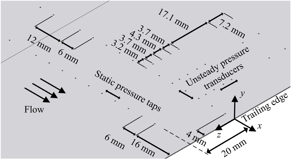
Figure 2. Distribution of static pressure taps and unsteady pressure transducers.
Alongside the unsteady pressure transducers, a total number of  $58$ pressure taps were fitted for static wall-pressure measurements along the streamwise direction and with a constant tap-to-tap distance of ${6}\ {\rm mm}$. The first tap is located ${16}\ {\rm mm}$ upstream of the trailing edge. Moreover, the pressure taps were mounted with an offset of ${20}\ {\rm mm}$ from the flat plate centreline and the lower lip line of the nozzle.
2.3. Finlet design
Although the investigated surface treatments have slightly different parameter assignments for instance for the total finlet and section lengths as well as the finlet trailing-edge geometry, their design largely resembles that presented by Afshari et al. (Reference Afshari, Azarpeyvand, Dehghan, Szöke and Maryami2019a), which is referred to as the conventional finlet design here. Figure 3 illustrates the design of the conventional finlets and the corresponding geometric parameters. They consist of identical walls of  ${0.5}\ {\rm mm}$ thickness oriented in the streamwise direction. The thin walls are arranged with a spanwise wall-to-wall distance of $S$. The symbols $L$ and $H$ designate the finlet length and the maximum finlet height, respectively. For the description of the local finlet height, the placement location of the finlet treatment is introduced as the distance, $X$, from its trailing edge to the trailing edge of the flat plate, as illustrated in figure 1. Since no scenarios are investigated, in which the finlets extend beyond the flat plate trailing edge, $X$ represents a positive number, whereas $x = -X$. To facilitate a smooth flow transition and avoid sudden changes to the boundary-layer characteristics, the leading edge of each wall structure is tapered and shaped proportional to the theoretical development of the boundary-layer thickness (Schlichting & Kestin Reference Schlichting and Kestin1979), as described in (2.1). The trailing edge of each wall structure is rounded with a radius equal to the maximum finlet height (Afshari et al. Reference Afshari, Azarpeyvand, Dehghan, Szöke and Maryami2019a). For ease of reference, the local finlet height, $\eta (x)$, is defined as
 \begin{equation} \eta (x) = \begin{cases} 0 & x < X - L, \\ a(x - X + L)^{4/5} & X-L \leqslant x \leqslant X-\left(L-(H/a)^{5/4}\right), \\ H & X-\left(L-(H/a)^{5/4}\right) < x < X-H, \\ \sqrt{H^2 - (x-X+H)^2} & X - H \leqslant x \leqslant X, \\ 0 & x > X, \end{cases} \end{equation}
as indicated in figure 3. In (2.1), the parameter  $a$ is introduced to keep the length of the tapered part constant at ${33}\ {\rm mm}$ independent from $H$. It was indicated in § 1 that one of the objectives of the present study is to shed light on the initiation of flow modifications and generation of turbulence structures through finlets at their leading edges. This shall be achieved by the investigation of the conventional finlets with the introduced leading-edge shape, providing a smooth flow transition into the treated area. Thereby, preliminary measurements in the course of the present investigations suggested that the smooth transition may as well be realised using a ramp-function approach. However, for better comparability with the work of Afshari et al. (Reference Afshari, Azarpeyvand, Dehghan, Szöke and Maryami2019a), the leading-edge shape of the conventional finlets is adopted. Different leading-edge shapes have also been investigated for instance by Gstrein, Zang & Azarpeyvand (Reference Gstrein, Zang and Azarpeyvand2021), where it has been shown that the profile of the conventional finlet treatment provides optimum conditions for the reduction of trailing-edge noise without drawbacks from treatment self-noise.
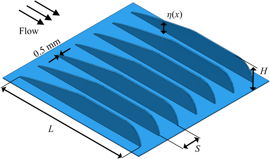
Figure 3. Finlet-treatment design and geometric parameters.
The finlet walls were produced by rapid prototyping and held upright in place by a  ${0.3}\ {\rm mm}$-thick substrate layer, which was then locally removed to uncover the pressure sensors beneath. For the present investigation, a large number of conventional finlet treatments with different geometric parameters were fabricated, with finlet lengths ranging from $L = {50}\ {\rm mm}$ to $L = {80}\ {\rm mm}$, different heights from $H = {6}\ {\rm mm}$ to $H = {20}\ {\rm mm}$ and spacing from $S = {2}\ {\rm mm}$ to $S = {12}\ {\rm mm}$. Preliminary experiments as a part of this work have shown that the finlet application is most efficient in reducing the trailing-edge noise when using a length of $L = {65}\ {\rm mm}$. Thus, the finlet length is kept at $L = {65}\ {\rm mm}$ for the present study. In the following, the finlet treatments will be named using the characteristic parameters, for instance, H12-S4 refers to the finlet treatment with $H = {12}\ {\rm mm}$, $S = {4}\ {\rm mm}$. The untreated flat plate (in other words, the scenario in which no finlets are applied) will be referred to as the baseline configuration, whereas finlet-treated configurations will be referred to as treated configurations.
2.4. Measurement principles and validations
To provide a first insight into the experiment, the measurement principles including the calibration procedures, post-processing techniques and uncertainties are described in this section. First, the beamforming array used to capture the far-field noise is detailed, followed by the results that confirm the noise-attenuation capability of the finlets and provide a first parameter study. Next, the principles for measuring the near-field pressure and velocity are discussed. Subsequently, the static pressure distribution, unsteady wall-pressure spectra and boundary-layer characteristics are validated and compared with the literature for the baseline configuration.
2.4.1. Far-field beamforming array and measurement results
To quantify the far-field noise, a beamforming array was mounted above the centre of the flat plate trailing edge at a height of  ${1.4}\ {\rm m}$ from the flat plate surface, as shown in figure 1. The beamforming array has $64$ Panasonic WM- $61$A microphones arranged along nine spiral arms extending from the centre. The microphones were found to have an uncertainty of ${1.5}\ {\rm dB}$ for a ${95}\,{\%}$ confidence level (Celik, Bowen & Azarpeyvand Reference Celik, Bowen and Azarpeyvand2020). Beamforming data were collected at a sampling frequency of ${2}^{15}\ {\rm Hz}$ for a duration of ${70}\ {\rm s}$. The time-series data were fast Fourier transformed with a Hanning window with ${50}\,{\%}$ overlap and a block size of ${4096}{}$ samples. The sound pressure level (SPL) of the trailing-edge noise was then calculated in $1/3$-octave frequency bands using the delay-and-sum algorithm implemented within the Acoular software package (Sarradj & Herold Reference Sarradj and Herold2017).
Figure 4 shows two noise contour maps from beamforming calculations for a centre frequency of  $f_c = {1122}\ {\rm Hz}$ for the baseline (see figure 4a) and the H12-S4 treatment applied at $X / L = 1.54$ (see figure 4b) at $U_\infty = {15}\ {\rm m}\ {\rm s}^{-1}$ (corresponding to a Reynolds number of $Re = {990\,000}{}$ based on the flat plate length). At each centre frequency of the $1/3$-octave bands, the SPL was integrated over an area covering the middle part of the trailing edge, where the noise source strength remains approximately constant, shown with dashed lines in figure 4. To validate the beamforming data, the beamforming response to a point source from a VISATON FRS $8$ speaker, excited at discrete frequencies from ${500}\ {\rm Hz}$ to ${4000}\ {\rm Hz}$, was compared with a simulation of the point source. The accuracy of the source strength from the beamforming measurement was verified by comparing the simulated and measured point spread functions with the frequency range ${500}\ {\rm Hz} < f < {4000}\ {\rm Hz}$. The data were determined to be valid between ${550}\ {\rm Hz}$ and ${3550}\ {\rm Hz}$ (the comparison is not shown here for the sake of brevity). Taking into account the calibration and post-processing errors, the measurement uncertainty of the beamforming array is estimated to approximately ${1.5}\ {\rm dB}$ below ${2500}\ {\rm Hz}$ and approximately ${2}\ {\rm dB}$ above (Yardibi et al. Reference Yardibi, Bahr, Zawodny, Liu, Cattafesta and Li2010).
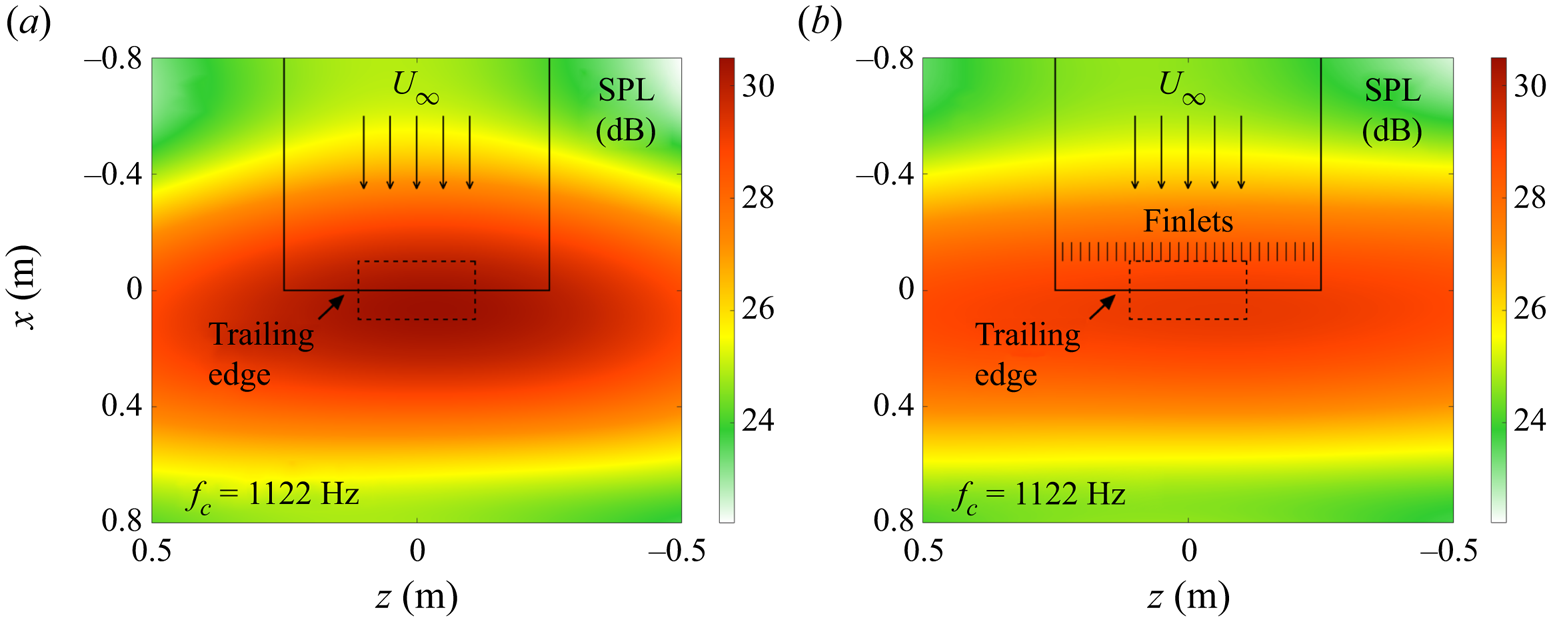
Figure 4. Beamforming contour maps with the outlines of the flat plate (solid lines) and source integration area (dashed lines): (a) baseline; (b) treated configuration.
The generated beamforming maps were used to obtain the far-field SPL spectra for the different configurations. Such far-field noise spectra have not yet been presented in the literature for finlets applied on a flat plate and serve as a confirmation of the finlets’ ability to reduce the trailing-edge noise. Furthermore, the measurements with varying finlet-placement location, finlet height and finlet spacing provide a parametric study, important for identifying the optimum parameter ranges for the more detailed investigations. Figure 5 shows the far-field SPL spectra obtained from the beamforming array over the frequency range from  ${570}\ {\rm Hz}$ to ${3540}\ {\rm Hz}$. The maximum overall reduction of ${3.5}\ {\rm dB}$ at ${1550}\ {\rm Hz}$ is observed for the H12-S2 finlet treatment with $H = {12}\ {\rm mm}$ and $S = {2}\ {\rm mm}$ when applied at $X / L = -1.54$, as shown in figure 5(c). Figures 5(a) and 5(b) suggest an optimal finlet location of $X / L = -1.54$ and an optimal finlet height of $H = {12}\ {\rm mm}$ for trailing-edge noise reduction. From the measured velocity profile (presented later in § 3.3), a boundary-layer thickness of ${17.95}\ {\rm mm}$ is determined for the baseline configuration in the finlet-application region. Indeed, Gstrein et al. (Reference Gstrein, Zang, Mayer and Azarpeyvand2022) earlier found that the most effective trailing-edge noise reduction on a NACA 0012 aerofoil by applying the finlet treatments upstream of the trailing edge was achieved with a finlet height of approximately ${70}\,{\%}$ of the boundary-layer thickness. This suggests that the finlets modify the boundary-layer characteristics upstream of the trailing edge, which eventually leads to the suppression of the trailing-edge noise.
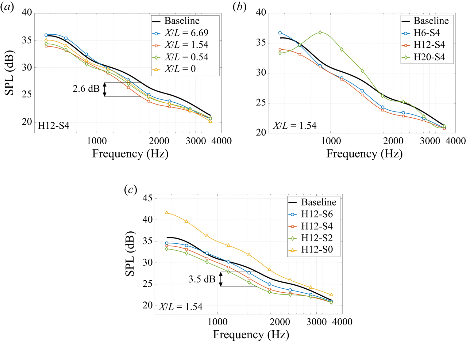
Figure 5. Far-field SPL for (a) H12-S4 configurations with different finlet-placement locations at  $Re = {990\,000}{}$, (b) configurations with different finlet heights at $Re = {990\,000}{}$ with $X / L = 1.54$, (c) configurations with different finlet spacing at $Re = {990\,000}{}$ with $X / L = 1.54$.
2.4.2. Static pressure measurement
To obtain the static wall pressure, the pressure information was transmitted through short brass tubes mounted beneath  ${0.4}\ {\rm mm}$ pinholes and connected to Chell Instrument $\mu$DAQ- $32$DTC pressure scanners via ${1}\ {\rm m}$-long polyurethane tubing. Data were sampled at ${1000}\ {\rm Hz}$ for a sampling duration of ${60}\ {\rm s}$. To characterise and validate the pressure distribution on the flat plate, five independent measurements were performed for the baseline configuration at a Reynolds number of $Re = {990\,000}{}$. For each set of measurements, both the time-averaged mean, $\mu$, and its standard deviation, $\sigma$, of the pressure coefficient were determined (Bendat & Piersol Reference Bendat and Piersol2010). Then, the overall mean values, $\bar {\mu }$, and the mean standard deviation, $\bar {\sigma }$, were derived. Figure 6 compares a single measurement of pressure coefficients, $C_p$, with the mean coefficient value and mean standard deviation. It can be clearly verified that the pressure gradient along the flat plate is essentially zero with a slightly negative mean pressure coefficient of $C_p = -0.0137$ and a mean standard deviation of ${0.0047}{}$. The maximum deviation occurs near the transition from the main plate to the bevelled trailing-edge part at $X / L = -1.15$.

Figure 6. A single measurement of the pressure coefficient distribution in streamwise direction for the baseline configuration, compared with the mean and the standard deviation.
2.4.3. Unsteady wall-pressure measurement
The unsteady wall-pressure fluctuations were sampled at a frequency of  ${2}^{15}\ {\rm Hz}$ for a sampling duration of ${70}\ {\rm s}$. Subsequently, the collected data were subjected to Welch's method with a Hamming window of $2^{12}$ samples and ${50}\,{\%}$ overlap to obtain the power spectral density (PSD) of the unsteady wall-pressure fluctuation spectra (referred to as wall-pressure spectra thereafter). The PSD result, $\phi _{pp}$, expressed in ${\rm dB}\ {\rm Hz}^{-1}$, was calculated as $\phi _{pp} = 10 \log _{10}{( S_{pp} (f)/ p^2_0 )}$, where $S_{pp} (f)$ is obtained from Welch's method and $p_0 = {20}\ {\mathrm {\mu }}{\rm Pa}$ is the reference pressure. Details of Welch's method can be found in the work of Bendat & Piersol (Reference Bendat and Piersol2010).
To validate the unsteady wall-pressure fluctuation measurements, the PSD spectra have been scaled by characteristic inner and outer boundary-layer variables and plotted against  $\omega \nu / u_\tau ^2$ and $\omega \delta _{b,0.99} / U_\infty$ as $10 \log _{10}{(S_{pp}(\omega ) u_\tau ^2 / \tau _w^2 \nu )}$ and $10 \log _{10}{(S_{pp}(\omega ) U_\infty / \tau _w^2 \delta _{b,0.99} )}$, respectively (Goody Reference Goody2004; Afshari et al. Reference Afshari, Azarpeyvand, Dehghan, Szöke and Maryami2019a). These variables are the shear stress at the flat plate surface, $\tau _w$, the friction velocity, $u_\tau = \sqrt {\tau _w/\rho }$, with the density of air, $\rho$, and the kinematic viscosity of air, $\nu$, at ${20}^{\circ }$. In addition, $\omega$ denotes the angular frequency in radians and $\delta _{b,0.99}$ the boundary-layer thickness at the flat plate trailing edge for the baseline configuration, which has been determined as the vertical distance from the flat plate surface at which the velocity, $u$, reaches ${99}\,{\%}$ of $U_\infty$. The velocity measurements used to determine the characteristic boundary-layer variables were obtained at the same location as the wall-pressure fluctuation measurements. To identify the local shear stress at the surface as $\tau _w = C_f \rho U_\infty ^2 / 2$, the skin friction coefficient, $C_f$, was estimated using the interpolation method established by Allen & Tudor (Reference Allen and Tudor1969). Furthermore, the wall-pressure spectra have been corrected based on Corcos’ correction factor (Corcos Reference Corcos1963) to account for the high-frequency attenuation due to the finite transducer sensing area. Figure 7 shows the corrected PSD spectra of the wall-pressure fluctuations closest to the trailing edge at $x / L = -0.06$ for ${10}\ {\rm m}\ {\rm s}^{-1}$, ${15}\ {\rm m}\ {\rm s}^{-1}$ and ${20}\ {\rm m}\ {\rm s}^{-1}$. Based on the convection velocity determined (as will be shown later), the present measurements have been found to satisfy $\omega r / U_c < 4$ in the frequency range of interest, as shown in figure 7.

Figure 7. The PSD of the wall-pressure fluctuation for the baseline configuration at  $U_{\infty } ={10}\ {\rm m}\ {\rm s}^{-1}$ $(Re = 660\,000)$, ${15}\ {\rm m}\ {\rm s}^{-1}$ $(Re = {990\,000}{})$ and ${20}\ {\rm m}\ {\rm s}^{-1}$ $(Re = {1\,320\,000}{})$: (a) scaled with inner boundary-layer variables; (b) scaled with outer boundary-layer variables. The accuracy criterion from Schewe (Reference Schewe1983), requiring that $\omega r / U_c < 4$, is also indicated for $U_{\infty } ={10}\ {\rm m}\ {\rm s}^{-1}$ (blue line with circles), $U_{\infty } ={15}\ {\rm m}\ {\rm s}^{-1}$ (orange line with squares), and $U_{\infty } ={20}\ {\rm m}\ {\rm s}^{-1}$ (green line with diamonds).
As indicated by Goody (Reference Goody2004) and demonstrated in figure 7, the wall-pressure spectra nearly coincide at high frequencies  $\omega \nu / u_\tau ^2 > 0.7$ if scaled by inner variables and at low frequencies $\omega \delta _{b,0.99} / U_\infty < 10$ if scaled by outer variables of the boundary layer. The spectral decay between $0.1 \leqslant \omega \nu / u_\tau ^2 \leqslant 0.3$ and $3 \leqslant \omega \delta _{0.99} / U_\infty \leqslant 10$ agrees well with the decay rate of $\omega ^{-0.7}$ reported by McGrath & Simpson (Reference McGrath and Simpson1987) and $\omega ^{-0.75}$ by Blake (Reference Blake1970), within a similar frequency range. The decay rate at high frequencies of $\omega \delta _{b,0.99} / U_\infty > 50$ or $\omega \nu / u_\tau ^2 > 1.5$ follows the $\omega ^{-5}$ decay rate reported in previous studies (Goody Reference Goody2004). The validation of the unsteady wall-pressure fluctuation data shows that the presented measurements at $Re = {990\,000}{}$ (i.e. $U_\infty = {15}\ {\rm m}\ {\rm s}^{-1}$) are well suited for investigating the energy–frequency characteristics of the turbulent boundary layer of the baseline and finlet configurations.
2.4.4. Hot-wire velocity measurements
For the boundary-layer velocity measurements,  $u$, a Dantec $55$P
$55$P $15$ single-wire probe was used and operated using a Dantec Streamline Pro system with a CTA $91$C
$91$C $10$ module. The miniature probe sensor has a sensing length of ${1.25}\ {\rm mm}$ and a diameter of ${5}\ {\mathrm {\mu }}{\rm m}$. To ensure that the probe is suitable for the present measurements, it is oriented such that the sensor span aligns with the spanwise direction in the flat plate coordinate system, conforming with the orientation during calibration. Due to the small probe dimensions, it can be smoothly fitted into the space between the finlet walls for treatments with a minimum finlet spacing of $S = {2}\ {\rm mm}$. Velocity scans of the $x$–
$x$– $z$ and $y$–
$y$– $z$ planes in the finlet wake were performed using Dantec $55$P
$55$P $51$ cross-wire probes to capture the streamwise, spanwise and wall-normal velocity components. However, a careful examination of the pressure–velocity correlation in the $x$–
$x$– $z$ and the $y$–
$y$– $z$ plane later reveals that the flow development and finlet-induced turbulence interaction can be well represented by the velocity fluctuations in the streamwise direction. Thus, for the sake of conciseness, only the streamwise components of the cross-wire measurements and the corresponding analysis are shown in the discussion. The velocity measurements were synchronised with the unsteady wall-pressure measurements at a sampling frequency of ${2}^{15}\ {\rm Hz}$ and a sampling duration of ${62}\ {\rm s}$ for the single-wire and ${16}\ {\rm s}$ for the cross-wire. All hot-wire probes were calibrated using a Dantec $54$H
$54$H $10$ calibrator.
The velocity fluctuation PSD was obtained applying Welch's method, similar to the approach for the wall-pressure fluctuation data. A logarithmic scale is used to present the velocity fluctuation PSD with  $U_\infty$ as the reference velocity, such that $\phi _{uu} = 10 \log _{10}{( S_{uu}(f) / U_\infty ^2 )}$. Thereby, $S_{uu}$ is directly obtained by applying Welch's method. Figure 8 compares the non-dimensional velocity, $u^+$, plotted against the non-dimensional wall distance, $y^+$, with Spalding's model (Spalding Reference Spalding1960) for the baseline configuration at ${10}\ {\rm m}\ {\rm s}^{-1}$, ${15}\ {\rm m}\ {\rm s}^{-1}$ and ${20}\ {\rm m}\ {\rm s}^{-1}$ at $x / L = -0.06$. Here, $u^+ = u / \sqrt {\tau _w / \rho }$ and $y^+ = y \sqrt {\tau _w / \rho } / \nu$ are the velocity and the wall distance related to wall units. It can be observed that the measured boundary-layer profiles agree well with Spalding's solution in the logarithmic region of $40 < y^+ < 300$.

Figure 8. Comparison of the non-dimensional velocity,  $u^+$, against the non-dimensional wall distance, $y^+$, for the baseline configuration at $U_{\infty }={10}\ {\rm m}\ {\rm s}^{-1}$, ${15}\ {\rm m}\ {\rm s}^{-1}$ and ${20}\ {\rm m}\ {\rm s}^{-1}$ with the model from Spalding (Reference Spalding1960).
The static pressure coefficient, wall-pressure spectra and boundary-layer profile results confirm that the flat plate produces a well-developed canonical turbulent boundary layer, appropriate for studying the fundamental flow effects induced by the finlets. Moreover, it can be observed that Reynolds number effects remain negligible at the three free stream velocities examined, corresponding to  $660\,000 \leqslant Re \leqslant 1\,320\,000$. Therefore, results from the pressure and velocity measurements will be presented at both $U_{\infty }={15}\ {\rm m}\ {\rm s}^{-1}$ and ${20}\ {\rm m}\ {\rm s}^{-1}$ in the following discussion to reveal the most representative turbulence characteristics. More specifically, the boundary-layer velocity (mean and fluctuations) and velocity-pressure cross-correlation ( $R_{up}$) are presented at $U_\infty = {20}\ {\rm m}\ {\rm s}^{-1}$ or a Reynolds number of $Re = 1\,320\,000$. All other pressure and wake measurements are presented at $U_\infty = {15}\ {\rm m}\ {\rm s}^{-1}$ or a Reynolds number of $Re = 990\,000$, since the wall-pressure spectra better capture the $\omega ^{-5}$ decay within the valid frequency range.
3. Boundary-layer characteristics of the baseline and treated configurations
The application of finlets leads to significantly altered turbulent boundary-layer characteristics within the treated area and the finlet wake. These modifications can be observed from the measurement results for the static pressure, wall-pressure fluctuations and velocity profiles, which are closely linked to the reduction of the trailing-edge noise of the flat plate.
3.1. Static wall-pressure coefficient
Figure 9 shows the development of the pressure coefficient,  $C_p$, (see figure 9a) and the root mean square (r.m.s.) of its fluctuations, $C_{p,{rms}}'$, (see figure 9b) from upstream of the treated area to the flat plate trailing edge. Results are presented for four different finlet treatments, namely S6, S4, S2 and S0. As the finlet height is kept constant at $H = {12}\ {\rm mm}$, the treatment configurations are denoted only with their respective spacing here and in the remainder of this work. The $C_p$ distribution modified by the finlets can be divided into three different regions, one of which is the section upstream of the treated area characterised through an adverse pressure gradient. This gradient intensifies with decreasing finlet spacing and reaches a maximum for the S0 finlet block. Immediately after the flow enters the treated area (in other words, the area between the finlet structures at $-2.54 < x/L < -1.54$), a favourable pressure gradient sets in, characterising the second region. Here, the pressure coefficient drops sharply, reaching a global minimum. In the transition region between the treated area and the finlet wake ( $-1.63 \leqslant x / L \leqslant -1.35$, as indicated in figure 9), the pressure coefficient quickly recovers to a level comparable to the one for the baseline configuration. This pressure recovery takes place over nearly identical distances for all finlet treatments except for the solid finlet block, regardless of the strength of the adverse pressure gradient upstream. The results for $C_{p,{rms}}'$, shown in figure 9(b), show a significant increase of the static pressure fluctuation compared with the baseline configuration in the front part of the treated area from $x / L = -2.46$ to $x / L = -2.28$, signifying an elevated level of fluctuations in the flow as it encounters the leading edges of the finlet walls. Subsequently, the static wall-pressure fluctuation returns to the baseline level. Downstream of the finlets, a considerable increase is evident only for the solid finlet block, which is likely to be due to flow separation and recirculation effects, reminiscent of a backward-facing step (Farabee & Casarella Reference Farabee and Casarella1984).

Figure 9. Pressure coefficient distribution,  $C_p$, and the r.m.s. of its fluctuations, $C_{p,{rms}}'$, for the baseline and the treated configurations from upstream of the treated area to the flat plate trailing edge: (a) $C_p$; (b) $C_{p,{rms}}'$.
The adverse pressure gradient upstream of the finlets, growing with decreasing finlet spacing, can be attributed to blockage and flow-recirculation effects in front of the leading edges of the finlet walls. This is concluded from the similar, though less pronounced pressure increase as for the solid finlet block, which also occurs upstream of a forward-facing step (Farabee & Casarella Reference Farabee and Casarella1984; Pearson, Goulart & Ganapathisubramani Reference Pearson, Goulart and Ganapathisubramani2013). However, the finlet effects are much weaker, as the bulk of the flow is channelled through the space between the walls. As the flow passes by the tapered leading edges, a favourable pressure gradient develops, seeking to compensate the pressure increase upstream. This phenomenon facilitates the quick recovery downstream of the treated area. A strong pressure increase ahead of the treated area is balanced by an even stronger pressure drop within. It is discernible from the static pressure data that turbulence structures likely arise in the front section of the treated area and the near wake of the finlets. This can be inferred from two salient characteristics. First, the elevated  $C_{p,{rms}}'$ in the front section of the treated area indicates stronger pressure fluctuations. Second, the quick $C_p$ recovery immediately downstream of the treated area as compared with the S0 scenario suggests a pressure compensation that is possibly initiated through turbulence mixing.
3.2. Unsteady wall-pressure spectra
The streamwise development of the wall-pressure fluctuation PSD,  $\phi _{pp}$, upstream of and within the treated area is presented in figure 10. The effects of the finlet treatments are immediately discernible from the increase of $\phi _{pp}$ at frequencies lower than ${1000}\ {\rm Hz}$ in front of and within the first half of the treated area, as shown in figures 10(a) and 10(b). A larger finlet spacing is found to produce a smaller $\phi _{pp}$ increase at low frequencies, as seen from figures 10(b) to 10(d), suggesting that the blockage effects from finlet application weaken as there is more space for the flow to be channelled through. It can further be inferred that the high energy content at relatively low frequencies is directly related to the interaction of the flow with the leading edges of the finlet walls. Moving downstream towards the end of the treated area, the low-frequency $\phi _{pp}$ increase diminishes, whereas in contrast, a decrease at frequencies higher than ${1000}\ {\rm Hz}$ of up to ${18}\ {\rm dB}\ {\rm Hz}^{-1}$ for the S2 configuration is discernible from figure 10(d). Afshari et al. (Reference Afshari, Azarpeyvand, Dehghan, Szöke and Maryami2019a) argued that the additional dissipation introduced by friction along the finlet walls can lead to the decrease of the wall-pressure fluctuation PSD at higher frequencies.

Figure 10. Development of the wall-pressure fluctuation PSD for the baseline and the treated configurations from upstream towards the end of the treated area: (a)  $x / L = -2.55$; (b) $x / L = -2.28$; (c) $x / L = -1.91$; (d) $x / L = -1.63$. The measurement location is indicated with a red circle in each inset.
Figure 11 shows the development of the wall-pressure fluctuation PSD in the finlet wake. Firstly, from the result for the S0 solid finlet block, the effects on the unsteady wall-pressure fluctuation associated with this scenario are identified. This configuration is characterised by a consistently higher  $\phi _{pp}$ level than that of the baseline configuration over the entire frequency range except at $x / L = -1.45$, particularly below ${200}\ {\rm Hz}$. The increase at frequencies below ${1000}\ {\rm Hz}$ here is clearly associated with the effects of a forward- and backward-facing step pair. These may be flow separation upstream of the treated area (Cherry, Hillier & Latour Reference Cherry, Hillier and Latour1984), the shedding of low-frequency large-scale vortex structures due to shear-layer separation and a recirculation bubble behind the step (Neto et al. Reference Neto, Grand, Métais and Lesieur1993; Furuichi, Hachiga & Kumada Reference Furuichi, Hachiga and Kumada2004; Nadge & Govardhan Reference Nadge and Govardhan2014), and possibly also flapping motions of the free, reattaching shear layer downstream of the step (Ma & Schröder Reference Ma and Schröder2017). The $\phi _{pp}$ decrease at frequencies above approximately ${300}\ {\rm Hz}$ compared with the baseline immediately downstream of the solid finlet block suggests reduced energy contents associated with high-frequency pressure fluctuations in the wake of the finlet block. Results from the solid finlet block offer plausible explanations of the observed $\phi _{pp}$ characteristics for the S2, S4 and S6 configurations. Immediately downstream of the treated area at $x / L = -1.45$, as shown in figure 11(a), all the finlets show an increase of the wall-pressure fluctuation PSD at frequencies below ${200}\ {\rm Hz}$. A second PSD hump can be identified between ${900}\ {\rm Hz}$ and ${2000}\ {\rm Hz}$, which is most pronounced for the S4 treatment but hardly noticeable for the S6 treatment. The first hump at ${200}\ {\rm Hz}$ resembles that observed for the solid finlet block, and hence, likely arises due to the large-scale turbulence structures associated with shear layers on top of the finlets (as also observed by Afshari et al. (Reference Afshari, Azarpeyvand, Dehghan, Szöke and Maryami2019a)) or recirculation bubbles downstream of the finlet walls. It will be referred to as turbulence shed from the top of the finlets. The nature of the second hump remains unclear at this point and will be further investigated in § 4.

Figure 11. Development of the wall-pressure fluctuation PSD for the baseline and the treated configurations from downstream of the treated area to the flat plate trailing edge: (a)  $x / L = -1.45$; (b) $x / L = -0.89$; (c) $x / L = -0.43$; (d) $x / L = -0.06$. The measurement location is indicated with a red circle in each inset.
Figures 11(b) to 11(d) show the unsteady wall-pressure spectra from the finlet wake to the flat plate trailing edge, which carry a trend similar to that shown by the results presented by Afshari et al. (Reference Afshari, Azarpeyvand, Dehghan, Szöke and Maryami2019a). Nevertheless, new insights can be obtained from the evolution of the wall-pressure fluctuation PSD upstream and within the treated area. Following the changes of the wall-pressure PSD shown in figures 10 and 11, the  $\phi _{pp}$ reduction remains much milder within the treated area as compared with that in the finlet wake, particularly for the S4 and S6 treatments. This suggests that the direct effect of channelling as defined by Afshari et al. (Reference Afshari, Azarpeyvand, Dehghan, Szöke and Maryami2019a) is not the only main reason for the strong reduction of $\phi _{pp}$ at frequencies higher than ${1000}\ {\rm Hz}$ at the flat plate trailing edge. To identify other mechanisms contributing to the unsteady wall-pressure fluctuation PSD attenuation in the finlet wake, further investigation of the boundary-layer characteristics will be presented in the following sections.
At this point, however, it is useful to compare the results for the wall-pressure spectra at the trailing edge with the far-field noise spectra (Amiet Reference Amiet1976). As expected, the results corroborate that all finlet treatments produce a consistent near- and far-field spectral reduction at  ${570}\ {\rm Hz} \leqslant f \leqslant 3540\ {\rm Hz}$. The S2 treatment is most effective in reducing both the near-field unsteady wall-pressure fluctuation and far-field trailing-edge noise, followed by the S4 and S6 treatments. Nevertheless, for frequencies lower than ${570}\ {\rm Hz}$, the far-field SPL indicates an upwards trend for the S2 treatment, which is also manifested from the low-frequency increase observed in $\phi _{pp}$, while the far-field SPL from the S4 and the S6 configurations remain below that of the baseline configuration at frequencies lower than ${570}\ {\rm Hz}$. Thus, the general trends observed for the near-field wall-pressure fluctuation agree very well with the far-field noise measurements within the valid frequency range.
3.3. Boundary-layer velocity and velocity fluctuation profiles
Figures 12 and 13 show the boundary-layer velocity,  $u$, normalised by the free stream velocity, $U_\infty$, as a function of the wall-normal distance, $y$. For ease of discussion, $y$ is normalised by the local finlet height, $\eta$, within the treated area and the maximum finlet height, $H$, farther upstream and in the finlet wake. The boundary-layer thickness, $\delta _{0.99}$, has been determined as the wall-normal distance to the flat plate surface at which $u = {0.99}{}U_\infty$. From the development of the velocity profiles shown in figures 12(a) to 12(d), it can be observed that the boundary-layer profiles of the S4 and S6 treatments remain comparable to that of the baseline configuration, though a minor increase of the boundary-layer thickness can be discerned upstream of the treated area. The increase of boundary-layer thickness corresponds well with the static pressure coefficient results, where an adverse pressure gradient builds up due to partial flow blockage from the finlet walls. On the other hand, the S2 treatment shows more drastic changes in the related velocity profile. Firstly, the S2 treatment produces a velocity deficit within the boundary layer as compared with the baseline configuration. Within the treated area at $x / L = -2.28$, as shown in figure 12(b), the velocity significantly decreases at $y / \eta = 1$, where the flow encounters the tapered leading edges of the finlet. Secondly, its velocity profile gradually develops an ‘S’-shaped kink close to the flat plate surface at $0 < y / \eta < 0.15$ at locations farther downstream (see figure 12c,d). The local velocity deficit within the boundary layer as the flow encounters the finlet wall structure and the recovery afterwards suggest a localised interaction between the flow and the finlet walls.

Figure 12. Development of the boundary-layer velocity profiles for the baseline compared with the treated configurations from upstream to the end of the treated area: (a)  $x / L = -2.55$; (b) $x / L = -2.28$; (c) $x / L = -1.91$; (d) $x / L = -1.63$. The measurement location is indicated with a red, dotted line in each inset and the boundary-layer thickness for the baseline case, $\delta _{b,0.99},$ marked with a black, dashed line.

Figure 13. Development of the boundary-layer velocity profiles for the baseline compared with the treated configurations from downstream of the treated area to the flat plate trailing edge: (a)  $x / L = -1.45$; (b) $x / L = -0.89$; (c) $x / L = -0.43$; (d) $x / L = -0.06$. The measurement location is indicated with a red, dotted line in each inset and the boundary-layer thickness for the baseline case, $\delta _{b,0.99},$ marked with a black, dashed line.
Figure 13 shows the development of the boundary-layer velocity profiles for the different configurations in the finlet wake. In general, the results show similar development trends to those discussed by Afshari et al. (Reference Afshari, Azarpeyvand, Dehghan, Szöke and Maryami2019a). The main observation to be noted here is that the boundary-layer is strongly altered in the finlet wake, where the S2 configuration induces the most significant boundary-layer growth except for the S0 finlet block and the highest near-wall velocity deficit. Since the S2 configuration has the smallest opening perpendicular to the free stream, these features are likely related with the more severe flow interaction with the finlet walls compared with the other configurations.
To understand whether the velocity deficit directly translates into reduction of the turbulence-energy content within the boundary layer, the r.m.s. of the boundary-layer velocity fluctuations,  $u'_{rms}$, is analysed. Figure 14(a) shows $u'_{rms}$ data for the baseline and the treated configurations at $x / L = -0.06$ to discuss different theories on the noise-reduction mechanism of finlets. The $u'_{rms}$ results for various configurations in the finlet wake have already been presented by Afshari et al. (Reference Afshari, Azarpeyvand, Dehghan, Szöke and Maryami2019a). However, from the clearly discernible decrease of the r.m.s. velocity fluctuation near the flat plate surface and its increase at $y / H \approx 1$ for the treated configurations compared with the baseline case, it is seen that turbulence intensity relocates from the surface to just above the finlet walls. This effect is increasingly pronounced as the finlet spacing decreases from $S = {6}\ {\rm mm}$ to $S = {2}\ {\rm mm}$. Bodling & Sharma (Reference Bodling and Sharma2019) interpreted this as the lifting of turbulence.

Figure 14. The r.m.s. of the boundary-layer velocity fluctuation,  $u'_{rms}$, at $x / L = -0.06$ for different finlet treatments and the baseline.
The finlet-induced changes of velocity and turbulence profiles observed in the boundary layer have a direct impact on the wall-pressure fluctuations and therefore the radiated trailing-edge noise. To investigate the cumulative effects of the modified boundary layer on the wall-pressure spectra, integrated velocity spectra based on the TNO model (Parchen Reference Parchen1998) were evaluated at  $x / L = -0.06$ close to the trailing-edge as $\phi _{int}(\omega ) = \int _{0.2 \delta }^{0.95 \delta } \overline {v'}^{2} ({\partial U}/{\partial x})^2 \phi _{vv}(\omega ) \,{{\rm d} y}$. Thereby, $v'$ and $U$ are the velocity fluctuation along the vertical direction and the mean velocity along the streamwise direction, respectively. Furthermore, $\omega$ denotes the angular frequency and $\phi _{vv}$ is the fluctuation spectrum for the vertical velocity component. The TNO model has been developed and widely used to predict trailing-edge noise from the boundary layer characteristics (Parchen Reference Parchen1998; Fischer, Bertagnolio & Madsen Reference Fischer, Bertagnolio and Madsen2017). Figure 15 shows the integrated spectra, $\phi _{int}$, for the baseline, the S2 and the S4 configurations (cross-wire measurements were not performed for the S6 case). Here, the length scale term considered by Parchen (Reference Parchen1998) and Fischer et al. (Reference Fischer, Bertagnolio and Madsen2017) is not included in the integration as no measurements of the vertical velocity component close to the flat plate surface were performed due to the spatial limitations using the cross-wire probe. Nevertheless, the integrated spectra show a consistent trend, indicating a clear spectral reduction for both the S2 and the S4 configurations at frequencies above approximately ${1500}\ {\rm Hz}$. The discrepancies can be attributed to the contribution of the different length scales, the changes in velocity fluctuation close to the flat plate surface, and the assumptions inherent in the TNO model. Hence, it is evident that the finlet-induced modifications to the boundary layer and its turbulence contents are directly linked to the reduction of wall-pressure spectra at mid-to-high frequencies, which in turn affects the far-field noise. In the following, the boundary-layer characteristics will be further investigated with pressure information to assess the mechanisms and determine the primary flow developments leading to the reduction of trailing-edge noise.

Figure 15. Comparison of the integrated velocity spectra based on the TNO model for the baseline, the S2 and the S4 configuration.
4. Characteristics of finlet-induced turbulence within the treated area
The results from § 3 indicate a strong interaction of the flow with the finlet walls. This in turn implies the generation of turbulence structures, which may be identified and traced using the velocity fluctuation PSD and the correlation between the unsteady wall-pressure and velocity fluctuations. The objective of this section is to perform a detailed coupled pressure–velocity analysis to elucidate the near-field finlet-induced turbulence and its effects on the wall-pressure spectra, spanwise coherence length and the associated far-field noise.
4.1. Modifications to the velocity fluctuation PSD
Figure 16 shows the development of the boundary-layer velocity fluctuation PSD from upstream to the end of the treated area for the S4 configuration. Results for the S2 and S6 treatments are not shown for the sake of brevity since they exhibit similar trends to the S4 configuration. As described in § 2.4.4, the velocity fluctuation PSD,  $\phi _{uu}$, is normalised using the free stream velocity $U_\infty$. For consistency in the $y$ coordinate, the distance from the flat plate surface is normalised by the local finlet height, $\eta$, within the treated area and by the maximum finlet height, $H$, upstream and downstream of the treated area. The results are presented as the difference from the treated to the baseline configuration, $\Delta \phi _{uu} = \phi _{uu,{treatment}} - \phi _{uu,{baseline}}$, for ease of comparison. Upstream of the treated area, as shown in figure 16(a), the difference in velocity fluctuation PSD between the treated and the baseline configuration is marginal. Entering the treated area, a sharp increase of $\Delta \phi _{uu}$ can be observed above the finlets within $1 \leqslant y / \eta \leqslant 3.5$ across almost the entire frequency range. Conversely, below $y / \eta = 1$, $\Delta \phi _{uu}$ is characterised by an area with negative magnitude, extending from ${20}\ {\rm Hz}$ to ${4000}\ {\rm Hz}$. Furthermore, a transition zone between positive and negative $\Delta \phi _{uu}$ (in other words, where $\Delta \phi _{uu} \approx 0$) forms along the finlet ridges at $y/\eta = 1$.

Figure 16. Development of the velocity fluctuation PSD difference,  $\Delta \phi _{uu}$, between the S4 and the baseline configuration from upstream towards the end of the treated area: (a) $x / L = -2.55$; (b) $x / L = -2.28$; (c) $x / L = -1.91$; (d) $x / L = -1.63$. The measurement location is indicated with a red, dotted line in each inset and the boundary-layer thickness for the treated configuration is marked with a black, dashed line.
The increase of  $\Delta \phi _{uu}$ due to finlet application indicates stronger velocity fluctuations in the region above the walls, where $\Delta \phi _{uu} \geqslant {3}\ {\rm dB}\ {\rm Hz}^{-1}$. The fluctuations right on top of the finlets likely originate from the interaction of the boundary-layer flow with the finlet ridges (top of the walls), which directly leads to the formation of turbulence structures. In contrast, the region of negative $\Delta \phi _{uu}$ at $y / \eta < 1$ reveals that the velocity fluctuation decreases within the flow bounded by the finlet walls (channelled flow), with the most significant decrease occurring close to the surface. The abated fluctuation in the region enveloped by the finlet walls suggests that turbulence dissipation through wall friction could play an important role. These effects are further corroborated by the fact that moving downstream within the treated area from $x/L = -2.28$ to $x/L = -1.63$, both the increase and decrease of $\Delta \phi _{uu}$ intensify with flow-ridge interaction and frictional dissipation continuously taking place. Moreover, the presence of finlet walls can help suppress the spanwise velocity fluctuations and contribute to the reduced $\phi _{uu}$. Nevertheless, for a zero-pressure-gradient turbulent boundary layer, the spanwise velocity fluctuations are significantly smaller than the streamwise fluctuations (Fernholz & Finleyt Reference Fernholz and Finleyt1996). The observed reduction of $\phi _{uu}$ is thus likely the consequence of combined effects on the streamwise as well as to the spanwise velocity fluctuations within the treated area. The velocity fluctuation PSD within the treated area confirm the argument put forward by Afshari et al. (Reference Afshari, Azarpeyvand, Dehghan, Szöke and Maryami2019a), who inferred dissipation effects from finlet wake measurements. Towards the end of the treated area, there is also an increase of $\Delta \phi _{uu}$ immediately below $y / \eta = 1.2$ at frequencies above ${4000}\ {\rm Hz}$ for the treated configuration, which is possibly due to the turbulence mixing between structures originating from the finlet ridges and those within the channelled boundary-layer flow.
Figure 17 shows the development of  $\Delta \phi _{uu}$ for the S4 treatment in the finlet wake from downstream of the treated area to the flat plate trailing edge. The result shown here provides some more insights that are not shown in the work of Afshari et al. (Reference Afshari, Azarpeyvand, Dehghan, Szöke and Maryami2019a). It is clear from the results that the finlet-induced turbulence structures forming on top of the ridges continue to exist in the finlet wake and are convected towards the flat plate trailing edge. However, the maximum level of the velocity fluctuation associated with these turbulence structures decreases from $\Delta \phi _{uu} \approx {8}\ {\rm dB}\ {\rm Hz}^{-1}$ at $x/L = -1.45$ to $\Delta \phi _{uu} \approx {5}\ {\rm dB}\ {\rm Hz}^{-1}$ at $x/L = -0.06$. Simultaneously, the finlet-induced turbulence formed close to the flat plate surface towards end of the treated area (see figure 16d) is convected away from $y / H \leqslant 0.5$ while its intensity decreases. This process is possibly driven by the mixing and merging of the turbulence from the channelled flow and that shed from the top of the finlets. Eventually, it leads to a strongly reduced $\Delta \phi _{uu}$ below $y / \eta \leqslant 0.8$ close to the flat plate trailing edge, as shown in figure 17(d), which also explains the strong decrease of $\phi _{pp}$ in the finlet wake as demonstrated in figure 11. In summary, the observed evolution of the velocity fluctuation in the finlet wake close to the surface is significant in several ways. First, it corroborates the observations from the wall-pressure fluctuation spectra, which show a notable reduction over a similar frequency range. The wall-pressure fluctuation spectra represent the cumulative effects of the velocity fluctuations in the boundary layer. From the results presented in § 3.2, it can be seen that the wall-pressure spectra generally decrease with the application of finlets, which corresponds well with the decrease of the velocity fluctuation PSD close to the flat plate surface. Second, it indicates that the mixing and evolution of the finlet-induced turbulence in the finlet wake can be beneficial to the reduction of the wall-pressure fluctuation and as a consequence can play an even more significant role for the overall noise-reduction than channelling. Third, it reveals an important aspect of finlet application, suggesting that the distance of the finlet to the flat plate trailing edge should be large enough to allow for sufficient development length for the turbulence-mixing process to reduce the wall-pressure fluctuation. This can be deduced from the continuously decreasing $\Delta \phi _{uu}$ near the flat plate surface as the measurement location moves from the treated area towards the flat plate trailing edge.

Figure 17. Development of the velocity fluctuation PSD difference between the S4 and the baseline configuration from downstream of the treated area towards the flat plate trailing edge: (a)  $x / L = -1.45$; (b) $x / L = -0.89$; (c) $x / L = -0.43$; (d) $x / L = -0.06$. The measurement location is indicated with a red, dashed line in each inset, and the boundary-layer thickness for the treated configuration is marked with a black, dashed line.
4.2. Autocorrelation and cross-correlation of pressure and velocity fields
To directly link the observed development of the turbulence structures with the wall-pressure fluctuation within the treated area, results for the pressure–velocity and the pressure–pressure cross-correlation as well as the pressure autocorrelation are presented next. To ease the discussion, the pressure–velocity and pressure–pressure cross-correlation will be referred to as  $p-u$ correlation and $p-p$ correlation, respectively. The non-dimensional $p-p$ cross-correlation coefficient, $R_{p_{i}p_{j}}$ is determined as $R_{p_{i}p_{j}} = E[p_{i}'(t) p_{j}'(t + \tau )] / (\sqrt {E[p_{i}'^2(t)]} \sqrt {E[p_{j}'^2(t)]})$. Here, $E$ represents the expected value and $\tau$ the time lag of the signal measured at transducer location $j$ to the signal measured at transducer location $i$. The prime symbol denotes the fluctuation (such that $p_{i}'$ is the pressure fluctuation at location $i$). The $p-u$ cross-correlation can be obtained by replacing the pressure signal $p_{j}'$ with the velocity signal $u_{j}'$. Furthermore, $U_\infty$ is used as the normalisation factor for the $p-u$ cross-correlation (instead of $\sqrt {E[p_{j}'^2(t)]}$) to account for the strong decrease of the velocity fluctuation above the boundary layer (Zang, Mayer & Azarpeyvand Reference Zang, Mayer and Azarpeyvand2020). It should be noted that the definition order matters, such that $R_{up} \neq R_{pu}$. From the $R_{up}$ results, it is possible to locate the primary region of correlation between the pressure and velocity fluctuations, which can identify the turbulence structures in the boundary layer modifying the wall-pressure field. Moreover, using the pressure autocorrelation, $R_{pp}$, the time scale of different turbulence structures can be identified, from which the length scales can be determined using the pressure cross-correlation results. The overall width of the autocorrelation peak directly accounts, to a fair degree of accuracy, for the size of the largest turbulence structures in the boundary layer and the initial rate of decay reveals the level of high-frequency energy content associated with the smaller turbulence structures (Glegg & Devenport Reference Glegg and Devenport2017).
Figure 18 compares the  $p-u$ correlation coefficients, $R_{up}$, with the pressure autocorrelation coefficients, $R_{pp}$ at two measurement locations in the front part of the treated area ( $x/L = -2.28$ and $-1.91$). The time lag, $\tau$, is non-dimensionalised by the free stream velocity, $U_\infty$, and the boundary-layer thickness at the trailing edge of the baseline configuration, $\delta _{b,0.99}$. The distance from the flat plate surface, $y$, is normalised by the local finlet height, $\eta$. The $R_{up}$ results are shown only for the S4 treatment since other treatments demonstrate similar trends. However, differences between the treatments with different finlet spacing can be identified from the $R_{pp}$ results. From figures 18(a) and 18(b), two isolated local $R_{up}$ maxima can be identified, one centred exactly at the finlet ridge at $y/\eta = 1$ and the other close to the flat plate surface with a time lag of $\tau \approx 0$. The first maximum at $y/\eta = 1$ is observed at a slightly negative time lag, meaning that the pressure fluctuation appears to precede the velocity fluctuation. Moving farther downstream from $x / L = -2.28$ to $x / L = -1.91$ (comparing figure 18a with figure 18b), the magnitude of $R_{up}$ near the flat plate surface becomes larger than that along the finlet ridge. In other words, there is a shift of the primary contribution of the velocity to the wall-pressure fluctuation from the turbulence generated along the finlets ridges to the channelled turbulence. Both local maxima of the $p-u$ correlation are followed by a field of anticorrelation, characterised as negative $R_{up}$. This is a clear sign of the finlet-induced turbulence being convected past the measurement locations.

Figure 18. Comparison of pressure–velocity cross-correlation coefficients,  $R_{up}$, and pressure autocorrelation coefficients, $R_{pp}$: (a) $R_{up}$ for S4 at $x / L = -2.28$; (b) $R_{up}$ for S4 at $x / L = -1.91$; (c) $R_{pp}$ for treatments with different spacing at $x / L = -2.28$; and (d) $R_{pp}$ for treatments with different spacing at $x / L = -1.91$. The pressure and velocity measurement location in (c,d) are marked with a red circle and a dotted, red line in the inset, respectively.
Further characteristics of finlet-induced turbulence can be identified from the  $R_{pp}$ results shown in figures 18(c) and 18(d). Firstly, the overall $R_{pp}$ peak width is larger at $x / L = -2.28$ (immediately downstream of the finlet entrance) than that at $x / L = -1.91$. From the wall-pressure spectra, a PSD increase at relatively low frequencies has been observed as the flow enters the treated area. The $R_{up}$ results from figure 18(a) reinforce the notion that the low-frequency increase in wall-pressure fluctuation PSD comes directly from the formation of turbulence structures along the finlet ridges. Thus, it is concluded that the pressure fluctuation at $x / L = -2.28$ experiences a stronger impact from the large-scale turbulence structures originating from the finlet ridges. Downstream of the finlet leading edges at $x / L = -1.91$, the turbulence induced by the flow interaction with the finlet leading edges, indicated by the maximum $R_{up}$, is still convected below the maximum finlet height ( $y / \eta \leqslant 1$). This is an important observation as it shows that the finlet-induced turbulence structures are channelled through the space between the finlets after they have been generated along the finlet ridges. Specifically, this means that the observed structures do not originate from boundary-layer turbulence lifted by the finlets, but rather from channelled turbulence generated along the finlet leading edges. Furthermore, the decreasing $R_{pp}$ peak width together with the change in the $R_{up}$ focus indicates that the large-scale turbulence decreases in size as it is also channelled and convected through the space between the finlet walls. Secondly, comparing the initial rate of decay between the baseline and treated configurations, it is found that the treatments generally effect much lower decay rates at both measurement locations, which indicates an overall reduction of small-scale turbulence in the boundary layer. Among the treatments, the S2 configuration exhibits the slowest decay rates. As discussed earlier, such a reduction may be attributed to turbulence dissipation due to surface friction along the finlet walls (Afshari et al. Reference Afshari, Azarpeyvand, Dehghan, Szöke and Maryami2019a).
Figure 19 compares the  $p-u$ correlation coefficients, $R_{up}$, with the $p-p$ correlation coefficients, $R_{p_ip_j}$, within the treated area. The measurement locations for the velocity and the wall-pressure fluctuations are staggered in space, which allows for tracking of finlet-induced turbulence in the streamwise direction and the associated convection velocity. In figures 19(a) and 19(b), the velocity fluctuations are measured at $x_i / L = -2.28$ near the entrance of the treated area, while the wall-pressure fluctuation is measured farther downstream within the treated area for both cases. The locations of the $R_{p_ip_j}$ measurements coincide with those of the $p-u$ correlation. Similar to the $R_{up}$ results shown in figure 18, two separate local correlation maxima can be observed for both $R_{up}$ and $R_{p_ip_j}$ from figures 19(a) to 19(d). Remarkably, the time lags associated with the two correlation peaks agree very well between the $p-u$ and $p-p$ correlations. The first $R_{up}$ peak observed in figure 19(a) occurs along $y / \eta = 1$ at small time lags of $0.2 \leqslant \tau U_\infty / \delta _{b,0.99} \leqslant 0.3$, whereas the associated $R_{p_ip_j}$ peak (see figure 19c) can be found at $\tau U_\infty / \delta _{b,0.99} = 0.2$. Both are marked with a solid circle. The second $R_{up}$ peak observed in figure 19(a) lies close to the flat plate surface at $1.7 \leqslant \tau U_\infty / \delta _{b,0.99} \leqslant 1.9$, with its associated $R_{p_ip_j}$ peak (see figure 19c) at $\tau U_\infty / \delta _{b,0.99} = 1.8$. These peaks are marked with solid rectangles. Similar observations can be made for $R_{up}$ and $R_{p_ip_j}$ with $x_j / L = -1.72$, as shown in figures 19(b) and 19(d).

Figure 19. Pressure–velocity ( $R_{up}$) and pressure–pressure ( $R_{p_ip_j}$) cross-correlation coefficients: (a) $R_{up}$ for S4 at $x_i / L = -2.28$ and $x_j / L = -1.91$; (b) $R_{up}$ for S4 at $x_i / L = -2.28$ and $x_j / L = -1.72$; (c) $R_{p_ip_j}$ for treatments with different spacing at $x_i / L = -2.28$ and $x_j / L = -1.91$, (d) $R_{p_ip_j}$ for treatments with different spacing at $x_i / L = -2.28$ and $x_j / L = -1.72$. The pressure and velocity measurement location in (c,d) are marked with a red circle and a dotted, red line, respectively.
The two separate peaks of the  $p-p$ and $p-u$ correlation coefficients reveal two distinct turbulence structures, which are convected through the treated area with noticeably different convection velocities. The turbulence structures corresponding to the smaller time lag are convected faster than those with the larger time lag, since they reach the downstream location of $x_j$ within a shorter period of time. Examining the time lags associated with each correlation peak, it becomes evident that the turbulence structures at $y / \eta = 1$, originating from the boundary-layer flow interaction with the finlet leading edges, travel at a faster bulk convection velocity than those in the channelled flow close to the flat plate surface. This can partly be explained from the $C_p$ and boundary-layer velocity profile results shown earlier, with the adverse pressure gradient at the front part of the treated area (see figure 9a) and the slower boundary-layer velocity close to the flat plate surface of the treated configuration (see figure 12).
Figure 20 shows the  $p-u$ and $p-p$ correlation coefficients between the locations of $x_i / L = -1.91$ and $x_j / L = -1.72$ towards the rear section of the treated area. From figure 20(a), a patch with $R_{up} \geqslant 0.005$ reaching from $y/H = 0$ to $y/H = 0.75$ can be observed at $\tau U_\infty / \delta _{b,0.99}\approx 0$, where the maximum occurs on the flat plate surface within $1 \leqslant \tau U_\infty / \delta _{b,0.99} \leqslant 1.2$. Unlike the $R_{p_ip_j}$ results at the upstream locations, the $p-p$ correlation coefficient in figure 20(b) shows a single peak for all the treatments considered, signifying the loss of correlation between the wall-pressure fluctuation and the turbulence structures along the finlet ridges. These observations may be explained by the ceasing direct interaction of the boundary-layer flow with the tapered finlet leading edges (due to their absence in this region). The turbulence close to finlet ridges experienced less surface-friction effects than the near-wall turbulence and hence was convected ahead of those in the channelled flow.
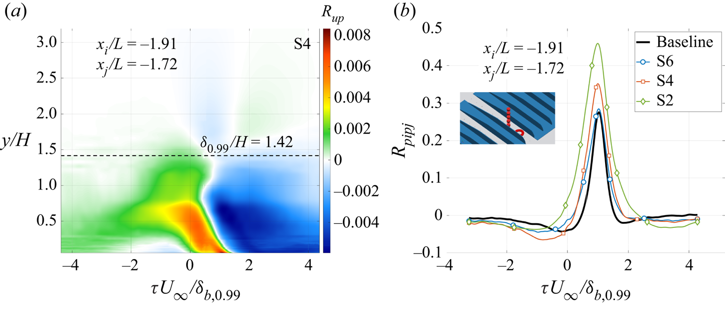
Figure 20. Pressure–velocity and pressure–pressure cross-correlation coefficients at  $x_i / L = -1.91$ and $x_j / L = -1.72$: (a) $R_{up}$ for S4; (b) $R_{p_ip_j}$ for treatments with different spacing. The pressure and velocity measurement location in (b) are marked with a red circle and a dashed, red line, respectively.
4.3. Convection velocity and streamwise length scale
Having indirectly discussed the convection velocity of turbulence structures in § 4.2, it is useful to determine the turbulence convection velocity close to the flat plate surface for the baseline and treated configurations. Figure 21 shows the convection velocity determined from the  $p-p$ correlation between adjacent pairs of transducers along the flat plate centreline and, in addition, the streamwise turbulence length scale, $\varLambda _x$. Following the study of Grizzi & Camussi (Reference Grizzi and Camussi2012), the convection velocity, $U_c$, is estimated as the ratio between the transducer separation distance, $\Delta x$, and the time lag, $\tau _{c,max}$, for the cross-correlation peak close to the baseline case (in other words, the turbulence being channelled); hence, $U_c = \Delta x / \tau _{c,max}$. The streamwise turbulence length scale, $\varLambda _x$, is determined as the product of the convection velocity, $U_c$ and the turbulence time scale, $\mathcal {T}$. The time scale can be found as $\mathcal {T} = \int _0^\infty R_{pp}(\tau ) \,{\rm d}\tau \approx \int _0^{\tau _0} R_{pp}(\tau ) \,{\rm d}\tau$, where $\tau _0$ is defined as the time lag at which the absolute value of the autocorrelation coefficient becomes less than ${0.0005}{}$. As shown in figure 21(a), the convection velocity for the baseline configuration is relatively constant at $U_c / U_\infty \approx 0.62$, agreeing well with the result from Afshari et al. (Reference Afshari, Azarpeyvand, Dehghan, Szöke and Maryami2019a). Within the treated area, the convection velocity for the treated configurations is comparable to the baseline case. Moving into the finlet wake, the convection velocity drops considerably to $U_c / U_\infty \approx 0.5$ and remains lower than the baseline up to the trailing edge. The convection velocity for the S2 configuration shows large fluctuations close to the exit of the treated area, where an intense turbulence mixing has been found to take place from the $\Delta \phi _{uu}$ results shown in figures 17(a) and 17(b) for the S4 case representative of other configurations. The strong fluctuation, not reported in the work of Afshari et al. (Reference Afshari, Azarpeyvand, Dehghan, Szöke and Maryami2019a), likely arises directly from the mixing and merging of turbulence from the channelled flow and shed from the finlet ridges. The development of the streamwise length scale, shown in figure 21(b), corroborates the previous findings that the large-scale turbulence forming both within the treated area and in the wake of the finlet treatment has significant impact on the wall-pressure fluctuation. Moreover, it can be observed that the streamwise length scale of the turbulence structures in the finlet wake increases with decreasing finlet spacing.
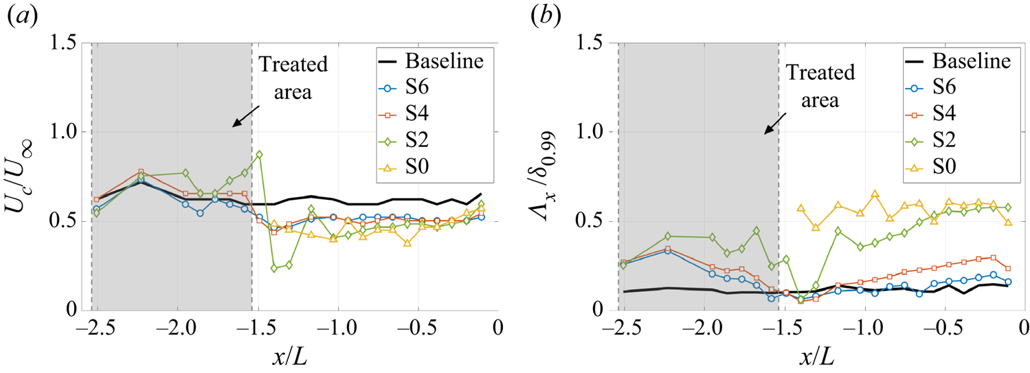
Figure 21. Development of the turbulence characteristics in the boundary layer from within the treated area to the trailing edge: (a) convection velocity; (b) streamwise turbulence length scale.
4.4. Spatiotemporal evolution of finlet-induced turbulence
By analysing the  $p-u$ correlation, $R_{up}$, across the streamwise ( $x$–
$x$– $y$) plane, the formation and convection of the finlet-induced turbulence along the finlet ridges and close to the flat plate surface can be traced as a function of the time lag, $\tau$. This is demonstrated for the baseline and treated configurations in figure 22. The $p-u$ correlations are determined between all the streamwise pressure transducers along the centreline and the velocity fluctuation measured at $x / L = -2.55$. Four time instances are selected to represent the spatiotemporal evolution of the turbulence structures. The complete turbulence evolution can be discerned from movie 1 in the supplementary material available at https://doi.org/10.1017/jfm.2023.33. For the baseline configuration, as seen from figures 22(a) to 22(d), a region with $R_{up} \approx 0.01$ can be observed moving in streamwise direction with increasing time lag. The angle between the flat plate centreline and the orientation of the highly correlated region steadily tilts from ${90}^{\circ }$ to about ${45}^{\circ }$. This illustrates how turbulence structures farther away from flat plate surface are convected faster than the near-wall turbulence.

Figure 22. Evolution of the turbulence structures within the treated area for the baseline and finlets (rows) at the different time lags (columns) of  $\tau _1 U_\infty / \delta _{b,0.99} = -0.3$, $\tau _2 U_\infty / \delta _{b,0.99} = 0.93$, $\tau _3 U_\infty / \delta _{b,0.99} = 1.63$ and $\tau _4 U_\infty / \delta _{b,0.99} = 1.96$: (a–d) baseline (B); (e–h) S6; (i–l) S4; and (m–p) S2 treatments.
For each treated configuration, a region with an elevated correlation ( $R_{up} \geqslant 0.03$), characterising the finlet-induced turbulence, first forms along the finlet leading edge. For the S2 treatment (see figure 22m–p), the centre of the correlated region develops along the outer edge of the finlet profile, trailing a region of negative $R_{up}$. In contrast, the S4 (see figure 22i–l) and S6 (see figure 22e–h) treatments show two separate turbulence-correlation regions with $R_{up} \geqslant 0.02$, which have distinct convection velocities. Unlike the turbulence structure in the S2 configuration, the dominant turbulence structures sink towards the flat plate surface, where they gradually merge and are then convected towards the end of the treated area. From figures 22(f) and 22(g) as well as 22(j) and 22(k), it can be seen that the two separate regions of high $R_{up}$ consist of one originating from the finlet ridge and the other likely originating from the channelled flow. It is also worthwhile to mention that, regardless of the finlet spacing, the elevated $R_{up}$ indicates that the dominant finlet-induced turbulence structures persist up to the end of the treated area and likely continue to exist and interact with turbulence in the finlet wake. The results presented in this section corroborate that the noise-reduction mechanism of finlets is related to the generation and channelling of finlet-induced turbulence rather than boundary-layer turbulence lifting.
5. Evolution of finlet-induced turbulence in the finlet wake
5.1. Pressure–velocity correlation in the finlet wake
Figures 23 and 24 illustrate the development of the finlet-induced turbulence in the wake of the S4 treatment, which is qualitatively representative of other finlet treatments. The cross-correlation coefficients,  $R_{pu}$, between the wall-pressure fluctuation at a single location and the streamwise velocity fluctuation measured along a dense grid in the $x$–
$x$– $z$ plane are presented in figure 23. Similar to figure 22, four instances of the time lag, $\tau _{ij}$, are shown to track the spatiotemporal evolution of the finlet-induced turbulence for each scenario (different pressure and velocity measurement locations) considered. Thereby, the index $i$ describes the scenario, whereas the index $j$ identifies the according different time lags. Movie 2 in the supplementary material illustrates the continuous evolution. Note that $z$-axis is normalised with $\Delta z / 2$, such that the finlet walls are at $\pm 1$, $\pm 3$, etc. Here, $\Delta z$ designates the finlet spacing plus the thickness of the walls. To capture the mixing of different turbulence structures as illustrated earlier, $p-u$ correlation data from different horizontal planes at $y / H = 1$ (see figure 23a–d) and $y / H = 0.3$ (see figure 23e–l) are considered. Furthermore, figures 23(i) to 23(l) differ from figures 23(e) to 23(h) in the reference wall-pressure location, as marked by the solid circle.

Figure 23. Pressure–velocity cross-correlation coefficients  $R_{up}$ in the finlet wake for the S4 treatment in the $x$-
$x$- $z$ plane at different measurement heights, $y/H$, and different wall-pressure measurement locations, $x / L$, at the time lags $\tau _{11} U_\infty / \delta _{b,0.99} = -6.34$, $\tau _{12} U_\infty / \delta _{b,0.99} = -5.23$, $\tau _{13} U_\infty / \delta _{b,0.99} = -2.99$, $\tau _{14} U_\infty / \delta _{b,0.99} = 0$, $\tau _{21} U_\infty / \delta _{b,0.99} = -11.69$, $\tau _{22} U_\infty / \delta _{b,0.99} = -3.23$, $\tau _{23} U_\infty / \delta _{b,0.99} = -2.49$, $\tau _{24} U_\infty / \delta _{b,0.99} = -0.25$, $\tau _{31} U_\infty / \delta _{b,0.99} = -4.73$, $\tau _{32} U_\infty / \delta _{b,0.99} = -2.99$, $\tau _{33} U_\infty / \delta _{b,0.99} = 0$ and $\tau _{34} U_\infty / \delta _{b,0.99} = 2.44$: (a–d) $y / H = 1$ and $x / L = -0.06$; (e–h) $y / H = 0.3$ and $x / L = -0.06$; (i–l) $y / H = 0.3$ and $x / L = -0.615$. The wall-pressure measurement locations are marked with a black circle.

Figure 24. Pressure–velocity cross-correlation coefficients  $R_{up}$ in the finlet wake for the S4 treatment in the $z$–
$z$– $y$ plane with the velocity measurement location $x / L = -1.35$ and different wall-pressure measurement locations at the time lags $\tau _{41} U_\infty / \delta _{b,0.99} = -1.74$, $\tau _{42} U_\infty / \delta _{b,0.99} = -0.87$, $\tau _{51} U_\infty / \delta _{b,0.99} = -4.73$ and $\tau _{52} U_\infty / \delta _{b,0.99} = -3.86$: (a,b) $x / L = -1.08$; (c,d) $x / L = -0.43$.
From figures 23(a) to 23(d), individual  $R_{pu}$ maxima of similar magnitude at $y/H = 1$ can be observed to be convected from the space between the finlet walls. As the flow structures travel downstream, they merge to form one spanwise-coherent region with a reduced $R_{pu}$ magnitude near the trailing edge. At a lower height of $y / H = 0.3$, two distinct physical phenomena can be observed from figures 23(e) to 23(h). Firstly, similar to its counterparts at $y / H = 1$, individual regions of positive $R_{pu}$ can be observed to emerge from the space between the finlet walls immediately downstream of the treated area. Secondly, a pair of positive and negative $R_{pu}$ regions occurs at approximately $x/L = -0.5$. As can be seen from figures 23(f) and 23(g), the turbulence emanating the treated area is convected towards the pair and merges with it. Subsequently, the merged turbulence travels towards the trailing edge in a coherent manner, as seen from figure 23(h).
In the earlier discussion of the finlet-induced turbulence within the treated area, two distinct turbulence structures, one from the finlet ridges and the other from the channelled flow, are found to have noticeably different convection velocities. The  $p-u$ correlation results in the finlet wake reinforce the theory that these turbulence structures undergo not only ‘self-merging’ between the separate finlet channels after exit, but also significant mixing with different turbulence structures present in the finlet wake. A very similar scenario can be observed in figures 23(i) to 23(l). Here, the wall-pressure measurement location is farther upstream at $x / L = -0.615$. It has been observed earlier that the wall-pressure spectra reduce across the entire frequency range for the treated configurations in the finlet wake, compared with the baseline case. The turbulence mixing and merging clearly benefits such a reduction, and, moreover, the process takes place relatively quickly, as seen from the $p-u$ correlation results. Thus, it can be reasonably argued that there exists an optimal distance of finlets to the flat plate trailing edge to most effectively reduce the trailing-edge noise.
Figure 24 captures the  $p-u$ correlation across the $y$–
$y$– $z$ plane behind the treated area at $x / L = -1.35$ to complement the measurements across the $x$–
$x$– $z$ planes and better illustrate the dynamics of turbulence mixing shortly after the treated area. Here, the $y$ axis is normalised with the boundary-layer thickness of the treated configuration. A complete time evolution of the $p-u$ correlation in $y$–
$y$– $z$ planes behind the treated area can be found in movie 3 in the supplementary material. The mixing of the turbulence being channelled through the finlets and that originating from the finlet ridges can be clearly observed, as shown in figures 24(a) to 24(d). Figures 24(a) to 24(d) show the $p-u$ correlation coefficients between the velocity fluctuation measured across the $y$–
$y$– $z$ plane at $x / L = -1.35$ and the wall-pressure fluctuations measured at $x / L = -1.08$ and $x / L = -0.43$, respectively. At the first time lag of $\tau _{41} U_\infty / \delta _{b,0.99} = -1.74$ in figure 24(a), individual structures can be identified near the flat plate surface in between the finlet walls, indicated with solid rectangles. As the time lag increases to $\tau _{42} U_\infty / \delta _{b,0.99} = -0.87$, as shown in figure 24(b), further structures separate from those at smaller time lag, emerge right above the finlet ridges. Similar observations can be made in figures 24(c) and 24(d). The $p-u$ correlation results firstly corroborate that the turbulence structures from the finlet ridges are convected faster than those from the channelled flow (note that the time lag is negative in this instance). Secondly, they indicate a loss of $p-u$ correlation with the channelled flow near the flat plate surface and an increase above the finlet height as the wall-pressure measurement location moves farther downstream, which in turn suggests more significant turbulence mixing between the two structures immediately downstream of the treated area.
Similar to figure 22 in § 4.4, figure 25 compares the development of the finlet-induced turbulence across the  $x$–
$x$– $y$ plane in the wake of the S2, S4 and S6 treatments with the baseline configuration. The $p-u$ cross-correlation in the finlet wake largely resembles that presented by Afshari et al. (Reference Afshari, Azarpeyvand, Dehghan, Szöke and Maryami2019a) and is shown here for a complete discussion of the turbulence-mixing and merging process. Thereby, the velocity measurements close to the trailing edge at $x / L = -0.06$ are correlated with the wall-pressure measurements along the flat plate centreline from upstream of the treated area towards the flat plate trailing edge. Again the time evolution of the finlet-induced turbulence across the $x$–
$x$– $y$ plane in the wake can be found in movie 4 in the supplementary material. The development of the $p-u$ correlation in the finlet wake shows that the turbulence that has formed at higher $y$ within the treated area is convected faster than the turbulence near the flat plate surface. This is seen from the inclination of either the positive or negative $R_{up}$ region. Comparing the finlet treatments with each other, the decreasing magnitude of $R_{up}$ close to the flat plate surface near the trailing edge with decreasing finlet spacing suggests greater turbulence mixing for finlet treatments with smaller spacing as the flow structures become less correlated through more extensive mixing.

Figure 25. Pressure–velocity cross-correlation coefficients in the finlet wake for different configurations (rows) at different time lags (columns)  $\tau _1 U_\infty / \delta _{b,0.99} = -6.63$, $\tau _2 U_\infty / \delta _{b,0.99} = -4.98$, $\tau _3 U_\infty / \delta _{b,0.99} = -2.32$ and $\tau _4 U_\infty / \delta _{b,0.99} = -0.66$: (a–d) baseline, (e–h) S6; (i–l) S4; and (m–p) S2 configuration.
5.2. Spanwise coherence length scale in the finlet wake
Aside from the modification of the unsteady wall-pressure fluctuation PSD, changes in the spanwise coherence length scale will also influence the scattered trailing-edge noise (Amiet Reference Amiet1976). This length scale here is introduced as the sum over the products of the unsteady wall-pressure fluctuation coherences,  $\gamma _i$, with the spanwise distances $z_i$. Thereby, the coherences, $\gamma _i$, are determined between the transducer with distance $z_i$ to the reference transducer at midspan, where $z_i$ is defined in § 2.2. Figure 26 shows the spanwise coherence length scale of turbulence, $\varLambda _z$, normalised with the boundary-layer thickness of the baseline at the trailing edge, $\delta _{b,0.99}$. The modifications to the spanwise coherence length scale through the finlets agree well with the results obtained by Afshari et al. (Reference Afshari, Azarpeyvand, Dehghan, Szöke and Maryami2019a). Nevertheless, having gained detailed knowledge of the flow evolution and mixing process of the finlet-induced turbulence, it is useful to also highlight several key observations from the spanwise coherence length scale results. The results confirm that the application of finlets and the finlet-induced turbulence-mixing process increase the turbulence length scale at low frequencies from within the wake of the finlets towards the trailing edge. Considering the correlation results shown in figure 23, where the turbulence structures appear to merge and extend over several finlet spacings, the significant increase of $\varLambda _z$ at low frequencies by more than the thickness of the boundary layer for the baseline case can be reasonably expected. On the other hand, the length scales gradually collapse onto each other at higher frequencies of $f\geqslant {600}\ {\rm Hz}$. Therefore, the significant reduction of wall-pressure fluctuations at higher frequencies as seen earlier translates directly to the reduction of trailing-edge noise (Amiet Reference Amiet1976). Furthermore, $\varLambda _z$ generally increases with decreasing finlet spacing, except for the solid finlet block. The increase of spanwise coherence length scale can be attributed to the more intense flow–finlet interaction and subsequent stronger turbulence mixing and merging in the finlet wake, where coherent structures from the top of the finlet walls as well as from the distinct channels between them merge and grow in size, as illustrated in figure 23.

Figure 26. Spanwise turbulence coherence length scale in the finlet wake near the trailing edge at  $x / L = -0.25$.
6. Summary and conclusions
Conventional finlet surface treatments have been mounted on a flat plate and thoroughly investigated with regard to their capability of trailing-edge noise reduction in extensive experiments in the aeroacoustics facility at the University of Bristol. From a large range of finlet treatments with distinct design parameters and placement locations with regard to the flat plate trailing edge, an optimum parameter analysis has been performed. With a beamforming approach, the reduction of trailing-edge noise through finlet-treatment application compared with the (untreated) baseline configuration has been corroborated, with an SPL reduction across the entire beamforming-frequency range and up to  ${3.5}\ {\rm dB}$ maximum reduction at ${1550}\ {\rm Hz}$ for the optimum parameter configuration. To further analyse the noise-reduction mechanism of the optimum finlet configuration, an in-depth investigation into the boundary-layer modifications arising from selected treatments has been performed. From the static and unsteady wall-pressure measurements, low-frequency turbulence structures have been identified in front of and immediately downstream of the treated area. At the trailing edge, the unsteady wall pressure PSD agrees well with the SPL measured for the considered treatments. On the basis of the boundary-layer velocity and profiles of the r.m.s. of the velocity fluctuations as well as the velocity fluctuation PSD, the flow has been found to be channelled through the space between the finlets and a mixing of the channelled turbulence with structures shed from the top of the finlet treatments has been observed at the end of the treated area and within the finlet wake. The connection of this finlet-induced turbulence with unsteady wall-pressure fluctuations and thus trailing-edge noise has been studied using pressure–velocity cross-correlations. The structures identified in front of the finlets have been found to be generated due to the flow interaction with the tapered finlet leading edges and subsequently convected downstream at the original surface distance of their formation. Thereby, the lower structures near the flat plate surface are convected more slowly, likely due to surface-friction effects along the finlet walls. The turbulence mixing has been observed from different layers above the flat plate surface in the three spatial directions, and has been found to increase the spanwise coherence length of the turbulence. As a result, the attenuation of trailing-edge noise has been associated with the near-wall decrease of turbulence intensity through viscous friction effects during the turbulence-mixing process within the finlet wake.
The present study has provided a detailed explanation of the trailing-edge noise-reduction mechanism of finlets applied on a flat plate. Although the boundary-layer characteristics have been investigated comprehensively, there are remaining questions to be addressed in prospective work. For instance, more detailed skin friction measurements can be performed to quantify the dissipation of turbulence through viscous friction within the treated area as well as in the finlet wake. Furthermore, despite of the few studies concerned with a variation of the finlet profile shape and the arrangement of wall structures in a staggered manner, effects of alternating profile shapes in the spanwise direction may be investigated more thoroughly to determine the most effective finlet arrangement for trailing-edge noise reduction. Finally, the knowledge of the modifications of the boundary-layer characteristics through finlets might facilitate follow-up works on the successful combination of finlets with other noise-reduction approaches such as serrated trailing edges.
Supplementary movies
Supplementary movies are available at https://doi.org/10.1017/jfm.2023.33.
Funding
This work was supported by the EU H2020 ARTEM project (grant number 769359).
Declaration of interests
The authors report no conflict of interest.


 Open access