2.1. Swept wing model, wind tunnel and flow stability

The experimental measurements presented in this work are performed using an in-house designed swept wing model extensively described in Serpieri & Kotsonis (Reference Serpieri and Kotsonis2015). The wing features a constant streamwise chord ($c=1273$ mm) and a sweep angle of $45^{\circ }$. A favourable pressure gradient characterizes the wing up to $x/c=0.63$ thus allowing thorough investigation of primary and secondary CFI and ensuing BL transition (Serpieri & Kotsonis Reference Serpieri and Kotsonis2016). Additionally, given the high sensitivity of CFI to surface roughness, the wing surface is carefully polished, ensuring a low and uniform roughness level ($R_q=0.2\ {\rm \mu}{\rm m}$, Serpieri & Kotsonis Reference Serpieri and Kotsonis2015).

The presented measurements are performed in the low-speed Low Turbulence wind Tunnel (LTT) at TU Delft, an atmospheric closed return tunnel featuring low free-stream turbulence level in the test section flow. Specifically, at the tested conditions the free-stream turbulence level is $T_u=0.025\,\%$ of the free-stream speed in the 2–5000 Hz frequency band (Serpieri Reference Serpieri2018). All measurements are performed at a fixed angle of attack ($\alpha =-3.36^\circ$) and various free-stream Reynolds numbers ($Re_{c}=1.35\times 10^6$, $1.85\times 10^6$, $2.17\times 10^6$). Stability solutions are computed for the three measured $Re_{c}$ based on a steady and incompressible solution of the 2.5-D BL equations and linear stability theory (LST, Mack Reference Mack1984). The procedure followed is extensively described in Serpieri (Reference Serpieri2018) and is omitted here for the sake of brevity. Referring to the $Re_c=2.17\times 10^6$ case, the computed stability solutions predict the wavelength and evolution of the most unstable mode ($\lambda _1=8$ mm), providing a reliable basis for the experimental forcing configurations design.

The $xyz$ reference system used in this work has its $x$ and $z$ axes orthogonal and aligned to the leading edge, respectively, with corresponding velocity components u, v, w. Throughout this work, the wall-normal direction (y) is non-dimensionalized by the experimentally measured unperturbed (i.e. no DRE applied) BL displacement thickness at $x/c=0.165$ for $Re_c=2.17\times 10^6$, hereafter defined $\bar {\delta }^*=0.46$ mm.

2.2. Spanwise periodic DRE

As previously discussed, numerous investigations dedicated to CFI apply DRE arrays on the wing surface towards focussing the BL development into a single monochromatic mode (e.g. Reibert et al. Reference Reibert, Saric, Carrillo and Chapman1996; Saric et al. Reference Saric, Reed and White2003). In the current application, the forced mode (i.e. the inter-spacing of the elements $\lambda _{{f1}}$) is chosen to coincide with the wavelength of the most unstable stationary CFI mode $\lambda _1$, corresponding to 8 mm, as predicted by LST and found in previous works (Serpieri Reference Serpieri2018). Typically, the DRE array is applied in the vicinity of the forced mode neutral point, thus close to the wing leading edge. However, recent investigations by the authors (Zoppini et al. Reference Zoppini, Westerbeek, Ragni and Kotsonis2022b) showed that this forcing configuration can be geometrically upscaled and moved at further downstream and experimentally more accessible chord locations. In particular, in the present measurements the DRE arrays are placed at $x_{DRE}/c=0.15$, where the unperturbed (i.e. no DRE applied) experimental BL displacement thickness is $\delta ^*=0.44$ mm (corresponding to $\delta _{99}=1.4$ mm). In comparison, the boundary layer thickness at $x/c=0.02$ is estimated to be $\delta ^*=0.14$ mm (corresponding to $\delta _{99}=0.6$ mm). While still extremely thin, the BL at $x/c=0.15$ is sufficiently thick to be measured by the high spatial resolution optical velocimetry technique used in this work. Additionally, the local growth rate of the modal CFI can be described by $\partial N/\partial x$, where $N$ is the $N$-factor evolution provided by the LST solution at $Re_c=2.17\times 10^6$. The $\partial N/\partial x$ value at $x/c=0.15$ is comparable to the value obtained in the vicinity of the dominant mode neutral point (i.e. within a 10 % difference), further validating the possibility of investigating the near-wake flow development for the downstream applied DRE array.

Various forcing configurations are investigated to characterize the receptivity of the near-element flow features to the DRE amplitude ($k$) and forcing wavelength ($\lambda _{{f1}}$). Specifically, four different element heights (nominally $k_1=0.1$ mm, $k_2=0.2$ mm, $k_3=0.3$ mm and $k_4=0.4$ mm) and three different forcing wavelengths are considered. Following the definition of $\lambda _i=\lambda _1/i$, forcing wavelengths $\lambda _{3/2} \simeq 5$ mm, $\lambda _1 \simeq 8$ mm and $\lambda _{2/3} \simeq 11$ mm are measured. Throughout this work, the $\lambda _1=8$ mm mode is associated with the most unstable mode at all considered Reynolds number cases. More specifically, stability solutions computed at the lower and higher $Re_c$ indicate that the most unstable CFI mode corresponds to wavelengths of 10 mm to 8 mm, respectively (Zoppini et al. Reference Zoppini, Westerbeek, Ragni and Kotsonis2022b). Hence, within the range of $Re_c$ investigated in this work, the $\lambda _1=8$ mm mode is either the most unstable mode or among the most unstable modes in the vicinity of $x_{DRE}/c$.

The DRE elements are manufactured in house by computer numeric controlled (CNC) laser cutting of a $100\ {\rm \mu}{\rm m}$ thickness self-adhesive black polyvinyl chloride (PVC) foil. Various heights can be obtained by pasting multiple layers of foil on top of each other prior to the cutting procedure. Each element is designed to be cylindrical with a diameter of $d=2$ mm, however, practical limits in the manufacturing process entail slight deviations in their actual shape. The elements have been fully characterized through a statistical study by using a scanCONTROL 30xx laser profilometer (405 nm wavelength and $1.5\ {\rm \mu}{\rm m}$ reference resolution) to extract their wavelength, diameter and height (table 2, Zoppini et al. Reference Zoppini, Westerbeek, Ragni and Kotsonis2022b).

The measured forcing configurations can be described through a purely geometrical scaling by defining the ratio between the DRE height ($k$) and the unperturbed BL displacement thickness at $x_{DRE}/c$ ($k/ \delta ^*$, Schrader et al. Reference Schrader, Brandt and Henningson2009). This parameter can be accompanied by the roughness Reynolds number $Re_{{k}} =({{{k}} \times |{\boldsymbol {u}}({{k}})|})/{\nu }$ (Gregory & Walker Reference Gregory and Walker1956; Reibert et al. Reference Reibert, Saric, Carrillo and Chapman1996) also accounting for the local BL evolution. Numerous investigations showed that the receptivity to roughness only depends on $k$ for small DRE amplitudes with a fixed diameter (Tempelmann et al. Reference Tempelmann, Schrader, Hanifi, Brandt and Henningson2012b; Kurz & Kloker Reference Kurz and Kloker2014). However, previous investigations by White et al. (Reference White, Rice and Ergin2005) showed that, for a 2-D BL, $Re_{{k}}^2$ offers a partial but valuable scaling of the near-element flow evolution. Additionally, $Re_{{k}}$ proves successful in predicting the criticality of the considered forcing configurations. In particular, in the present work configurations featuring $Re_{{k}}\geqslant 200$ behave super-critically (Zoppini et al. Reference Zoppini, Westerbeek, Ragni and Kotsonis2022b), therefore they are only considered in § 4 dedicated to the characterization of the near-element features of super-critical amplitude DRE. The geometrical parameters corresponding to the investigated forcing cases are reported in figure 1. A correlation of the considered cases to previous investigations can be obtained using the Von Doenhoff & Braslow (Reference Von Doenhoff and Braslow1961) diagram, relating the critical roughness Reynolds number to the inverse aspect ratio of the forcing elements (i.e. $d/k$) in 2-D base flows. For the sake of conciseness, a direct graphical comparison is omitted, however, the reference critical and super-critical cases (i.e. $Re_c=2.17\times 10^6$ with DRE amplitude $k_3$ or $k_4$) respectively correspond to $d/k=6.7$, 5 and $\sqrt {{Re}_{k}}=13.8$, 18.1. Hence, the critical case falls on the lower bound of the transitional region identified by Von Doenhoff & Braslow (Reference Von Doenhoff and Braslow1961), while the super-critical case falls well inside it.

Figure 1.

Geometrical parameters of the measured forcing configurations computed from numerical BL solutions. Colour map based on $k/\delta ^*$, symbols based on DRE height, legend indicating nominal element height [mm].

2.3. Dual-pulse tomographic PTV

The 3-D velocity distribution in the DRE vicinity is acquired through specialized high-resolution dual-pulse tomographic PTV (Malik & Dracos Reference Malik and Dracos1993; Wieneke Reference Wieneke2012; Schanz, Gesemann & Schröder Reference Schanz, Gesemann and Schröder2016). The measured 3-D domain is centred at $x/c=0.165$ and extends for almost $x/c=0.027$, $y/\bar {\delta }^*\simeq 6$ and $z/\lambda _1=3.5$ in the streamwise, wall-normal and spanwise directions, respectively.

The 3-D measurement volume is illuminated with a Quantel Evergreen Nd:YAG dual cavity laser (200 mJ pulse energy at $\lambda =532$ nm), optically accessing the test section through a Plexiglas window on the test section floor. Through a suitable optical arrangement, the laser beam is shaped into a 40 mm wide and almost 4 mm thick sheet parallel to the wing surface in the area of interest. The flow is imaged through 4 sCMOS LaVision Imager cameras ($2560\times 2160$ pixel, 16-bit, $6.5\ {\rm \mu}{\rm m}$ pixel pitch), installed on the outer side of the test section with a tomographic aperture of approximately $45^{\circ }$. Each camera is equipped with a 200 mm lens, a 2X teleconverter and a lens-tilt mechanism adjusted to comply with the Scheimpflug condition. The resulting focal length is 400 mm for each camera, featuring an aperture number $f_{\#}=11$ to keep the particles in focus throughout the entire volume depth. The distance between the imaged plane (i.e. the model surface) and the camera sensors is $\simeq$1 m, resulting in a magnification factor of $\simeq$0.41 and spatial resolution of $67\ {\rm px}\ {\rm mm}^{-1}$. The flow is seeded by dispersing $0.5\ {\rm \mu}{\rm m}$ droplets of a water–glycol mixture in the wind tunnel circuit.

For each investigated configuration, 4000 image pairs are acquired at a frequency of 15 Hz. The time interval between paired images is set to $8\ {\rm \mu}{\rm s}$, corresponding to a free-stream particle displacement of almost 10 px. A dual layer target is used for calibrating the tomographic imaging system, further correcting the obtained mapping functions using the volume self-calibration procedure (Wieneke Reference Wieneke2008; Schanz et al. Reference Schanz, Gesemann, Schröder, Wieneke and Novara2012). The resulting calibration uncertainty is $\simeq$0.04 px. The image pairs are processed in LaVision DaVis 10 through a shake-the-box, 2-pulse algorithm (Wieneke Reference Wieneke2012; Schanz et al. Reference Schanz, Gesemann and Schröder2016) estimating the 3-D velocity field within the acquired volume. The LaVision DaVis 10 processing also provides an estimate of the velocity uncertainties (Janke & Michaelis Reference Janke and Michaelis2021), which for the present case average to 1.8 % of the local velocity in the BL region. An in-house developed Matlab routine is then employed to perform trajectory binning and conversion to a Cartesian grid. The final vector spacing results in approximately 0.25 mm in the $xz$ plane and 0.04 mm along the $y$-direction.

2.4. Velocity field reconstruction and processing

The time-averaged ($\bar {u}, \bar {v}, \bar {w}$) and standard deviation ($u', v', w'$) velocity fields are obtained for all three velocity components in the $xyz$ domain. For the sake of conciseness, the main data processing techniques adopted throughout this work are hereafter briefly described as applied to $\bar {u}$, while the treatment of $\bar {v}$ and $\bar {w}$ follows a similar procedure. The wall-normal BL velocity profile ($\bar {u}_b$) is estimated by averaging the $\bar {u}$ velocity signal along $z$ for each fixed $xy$ location. At each chordwise location, the free-stream velocity $\bar {u}_{\infty }$ is estimated as the average of $\bar {u}_b$ for $y>\delta _{99}$ and its value at $x/c=0.165$ is used to non-dimensionalize the three velocity components. The disturbance velocity field ($\bar {u}_d$) is computed at each ($x,y_*,z$) as $\bar {u}_d =\bar {u}(x,y_*,z) - \bar {u}_b(x, y_*)$, with $y_*$ representing a fixed wall-normal location. The analysis of such velocity fields allows for the extraction of the amplitudes of the high- and low-speed streaks (Andersson et al. Reference Andersson, Brandt, Bottaro and Henningson2001). The wall-normal disturbance velocity profile ($\langle \bar {u} \rangle _z$) is computed as the root mean square of the $\bar {u}_d$ velocity signal along $z$ (Reibert et al. Reference Reibert, Saric, Carrillo and Chapman1996; Tempelmann et al. Reference Tempelmann, Schrader, Hanifi, Brandt and Henningson2012b). Furthermore, a spatial fast Fourier transform (FFT) analysis is performed on the spanwise velocity signal at each $xy$ location (${\rm FFT}_z(\bar {u})$), characterizing the BL spectral composition as well as the development of the dominant spanwise mode and its harmonics. This allows for the computation of the total and the modal (i.e. per individual FFT mode) instability amplitude by integrating respectively $\langle \bar {u} \rangle _z$ or the individual FFT mode shape functions along $y$ up to the local BL $\delta _{99}$ (Reibert et al. Reference Reibert, Saric, Carrillo and Chapman1996; Downs & White Reference Downs and White2013). This provides an estimation of the velocity disturbances’ growth and evolution along the airfoil chord. Following White et al. (Reference White, Rice and Ergin2005), the CFI energy is instead computed as $E(\bar {u})=\int _0^{\delta _{99}} (\langle \bar {u} \rangle _z)^2 \,{{\rm d} y}$. The summation of the disturbance energy associated with each of the three velocity components provides the total disturbance energy $E(\bar {{\boldsymbol {u}}})$. Similar processing is applied to the individual FFT shape functions to compute the modal energy evolution.

By considering all three velocity components available through the tomographic PTV measurement, the 3-D coherent structures dominating the near-wake flow are identified by applying a vortex identification criterion, namely the $Q$-criterion (Hunt, Wray & Moin Reference Hunt, Wray and Moin1988). The flow field is first decomposed into its spectral components and is reconstructed accounting for a truncated set of Fourier modes to improve the data signal-to-noise ratio. The reconstructed domain includes the statistically represented flow field incurred by one DRE element and is rotated to obtain a reference frame ($x_R, y_R, z_R$) with $x_R$ aligned with the crossflow vortex axis, $y_R$ coincident with y, and $z_R$ normal to the $x_Ry_R$ plane. The corresponding time-averaged velocity components are named $\bar {u}_R$, $\bar {v}_R$, $\bar {w}_R$.

3.1. Stationary disturbance topology

Direct characterization of the near-element flow topology and dominant stationary disturbances is obtained through the time-averaged and standard deviation velocity fields. The critical wavelength forcing configuration (i.e. $\lambda _{{f1}}=\lambda _1$) at $Re_{{k}}=192$ is considered hereafter as the baseline case for the stationary flow topology investigation. The corresponding disturbance velocity field ($\bar {u}_d$) is reported in figure 2(a–c), while figure 2(d–f) presents the temporal standard deviation contours ($u^{\prime }$).

Figure 2.

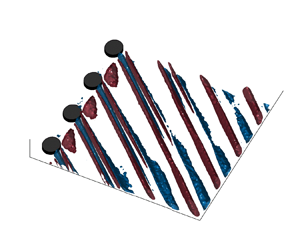
(a–c) Values of $\bar {u}_d$ and (d–f) $u^{\prime }$ for forcing case $\lambda _{{f1}}=\lambda _1$, $Re_{{k}}=192$ (for $k_3$) in (a,d) the $xz$ plane at $y=0.55\bar {\delta }^*$; (b,e) the $yz$ plane at $x_1=0.154c$ (vertical dashed line in a,d) and (c,f) at $x_2=0.174c$ (vertical dash-dot line in a,d). Disturbance profiles at (h) $x_1$ and (i) $x_2$ for all three velocity components; element height (solid horizontal black line); LST $\lambda _1$ shape function (dashed grey line) scaled to match $\langle \bar {u} \rangle _z$ maximum; element height (horizontal full line).

Owing to the volumetric measurement, the stationary flow features dominating the near-element flow evolution can be identified in both the $xz$ and $yz$ planes. Specifically, the velocity contours in figure 2(a–c) reveal a low-speed streak developing aft of each DRE in correspondence to the element's wake. This low-speed region is accompanied by two high-speed streaks developing on its flanks. The resulting streak alternation corresponds well to the horseshoe vortex legs wrapping around and extending aft of the element, identified by previous investigations (Baker Reference Baker1979; Kurz & Kloker Reference Kurz and Kloker2016). In between neighbouring roughness elements the incoming BL maintains a laminar behaviour as the velocity disturbances introduced by each DRE are highly localized in correspondence to the individual element's wake. The identified stationary flow topology closely resembles the near-element flow of isolated DRE in 2-D or 3-D BLs (e.g. Baker Reference Baker1979; Loiseau et al. Reference Loiseau, Robinet, Cherubini and Leriche2014; Bucci et al. Reference Bucci, Cherubini, Loiseau and Robinet2021; Zoppini et al. Reference Zoppini, Ragni and Kotsonis2022a). This is also in agreement with the findings of Von Doenhoff & Braslow (Reference Von Doenhoff and Braslow1961), in which the near-element behaviour of the individual elements of a DRE array was found to be comparable to that of an isolated DRE if they are arranged at a wavelength $\lambda _{{f1}}>3d$. Nonetheless, due to the presence of the crossflow velocity component in the base flow, the stationary structures identified in the near-element flow region follow an asymmetric downstream development (Kurz & Kloker Reference Kurz and Kloker2016; Brynjell-Rahkola et al. Reference Brynjell-Rahkola, Shahriari, Schlatter, Hanifi and Henningson2017; Zoppini et al. Reference Zoppini, Ragni and Kotsonis2022a). In particular, in figure 2(a) the outboard high-speed streak (denoted by a solid line) is decaying in the downstream direction and is substituted by the development of an outboard low-speed streak (denoted by a dash-dot line). Instead, the inboard high-speed streak (indicated by a dashed line) persists until the end of the acquired domain albeit decreasing in amplitude. This results in a far-wake flow dominated by an almost periodic alternation of high- and low-speed regions, respectively induced by the evolution of the inboard high-speed streak and the merging of the outboard low-speed streak and the low-speed wake. The ensuing BL velocity modulation is a typical feature of a modal stationary CFI, resulting from the momentum redistribution across the BL induced by the crossflow vortices (figure 2(c), Bippes Reference Bippes1999; Saric et al. Reference Saric, Reed and White2003). Based on the observed development, a near-wake flow region can be defined (i.e. $x/c<0.164$), which is mostly affected by the stationary streak structures development, while the far-wake flow region (i.e. $x/c>0.164$) is mostly dominated by modal CFI development (as further discussed in figure 7). Furthermore, the identified streak structures develop by following a constant phase trajectory which is oriented at an angle of ${\simeq }6^{\circ }$ towards the inboard direction with respect to the free-stream flow (i.e. the $X$ direction). This mild tilting compares well with the angle forming between developing stationary crossflow vortices and the free-stream velocity in the same set-up at more downstream chord locations, as experimentally measured and predicted by LST (Serpieri Reference Serpieri2018).

The standard deviation fields reported in figure 2(d–f) indicate that in the element vicinity the regions of higher unsteadiness are mostly located in correspondence to the identified streak structures. In particular, stronger unsteady velocity fluctuations appear at the interface between the outboard low-speed and high-speed streaks, representing a local high (mostly spanwise) shear region (Klebanoff et al. Reference Klebanoff, Cleveland and Tidstrom1992; Kuester & White Reference Kuester and White2015; Berger & White Reference Berger and White2020). This suggests that the near-wake disturbances onset and downstream evolution are strongly related to the wall-normal and spanwise shear layers induced by the recirculation region developing in the element's wake (figure 2(e), Brynjell-Rahkola et al. Reference Brynjell-Rahkola, Shahriari, Schlatter, Hanifi and Henningson2017; Zoppini et al. Reference Zoppini, Ragni and Kotsonis2022a). The overall level of unsteady fluctuations reduces further downstream accompanied by the progressive weakening of the streaks structures. Additionally, as the flow structures evolve downstream of the higher-fluctuation regions locally shift in correspondence to the inboard high-speed streak. Despite the observed early rise of strong unsteady disturbances, the overall transition scenario occurring in the present case appears to be driven by a typical modal CFI breakdown, as revealed by global thermography-based imaging (not shown here for brevity). Hence, it can be expected that the unsteady fluctuations detected at the end of the imaged domain further decay downstream.

Stationary disturbance velocity profiles ($\langle \bar {u} \rangle _z$) are extracted at two representative chord locations $x_1/c=0.154$ and $x_2/c=0.174$ (figure 2h,i). The reduction of the disturbance profile amplitude at $x_2$ reflects the weakening of the streak structures at more downstream locations. In addition, the developing flow disturbances are observed to grow in size along the wall-normal direction, as their maximum value moves from $y=0.55\bar {\delta }^*$ to $y=1.05\bar {\delta }^*$. This effect is evident in the $yz$ plane $\bar {u}_d$ and $u^{\prime }$ contours, and can be related to the natural thickening of the BL as well as to the development of the modal CFI downstream of $x/c=0.164$ (Saric et al. Reference Saric, Reed and White2003). Specifically, at $x_1$ (figure 2b,e,h) the velocity streaks developing in the element vicinity only affect the near-wall BL region, reaching the amplitude peak value at a wall-normal distance comparable to the element height. On the contrary, the downstream evolution of the developing structures (figure 2c,f,i) affects the whole BL wall-normal extent through the well-known momentum modulation associated with the CFI development (Bippes Reference Bippes1999; Saric et al. Reference Saric, Reed and White2003). Nonetheless, the absence of a secondary lobe in the disturbance velocity profiles and the relatively low maximum amplitude of the stationary disturbances ($\langle \bar {u} \rangle _z<0.05\bar {u}_\infty$) indicate a largely linear evolution of CFI within the investigated domain. This is reflected in the close match between $\langle \bar {u} \rangle _z$ and the numerically computed local LST shape function for the $\lambda _1$ mode evolution (figure 2i).

Overall, both the $\bar {u}_d$ contours and $\langle \bar {u} \rangle _z$ profiles in figure 2 show that the streak structures developing in the near-wake region undergo an initial growth phase while decaying shortly downstream. The behaviour of the individual streaks can be quantified by extracting the streak amplitude ($A_{str}$), estimated as the maximum (minimum) $\bar {u}_d$ value for the high- (low-)speed streaks, respectively. The resulting $A_{str}$ is reported in figure 3(a) for three $Re_{{k}}$ configurations obtained by modifying the DRE array amplitude. Both in $Re_{{k}}=192$ and $Re_{{k}}=90$ cases the high-speed streaks feature an initial growth phase followed by subsequent decay which is more evident for the higher-amplitude forcing. The low-speed streak is instead showing a monotonic decay of the absolute amplitude value. Similar behaviour is seen for the lowest forcing amplitude considered (i.e. $Re_{{k}}=21$). However, the measurement accuracy in this case is hindered by the overall weaker amplitude values, therefore this configuration is disregarded in the remainder of this work.

Figure 3.

Streak amplitude analysis for varying $Re_{{k}}$: (a) $A_{str}$ for high-speed (full line) and low-speed (-.) streaks; (b) $A_{And}$ and amplitude limit for laminar streak breakdown (-., Andersson et al. Reference Andersson, Brandt, Bottaro and Henningson2001). Element location (shaded grey region).

In addition to the localized amplitude estimations, a relative streak amplitude metric is defined as $A_{And}=0.5\times (\max (\bar {u} _d) - \min (\bar {u} _d))$ based on the criterion introduced by Andersson et al. (Reference Andersson, Brandt, Bottaro and Henningson2001). The resulting estimation is reported in figure 3(b) and shows that the initial growth phase and subsequent decay concentrate within comparable chordwise extent for the two higher $Re_{{k}}$ considered. Additionally, based on the $A_{And}$ definition Andersson et al. identified a critical streak amplitude value of approximately $0.2\bar {u}_{\infty }$ as a sufficient onset condition for laminar breakdown of the developing velocity streaks in 2-D BLs. This value is not reached in the presented cases, in agreement with the laminar evolution of the flow structures observed in figure 2 and confirming the $Re_{{k}}$ predictions. Nonetheless, the relatively high initial amplitude of the induced near-wake disturbances (especially in case $Re_{{k}}=192$) can lead to increased unsteadiness and enhanced shear layer development in the element near-wake flow, as shown in figure 2(e).

Capitalizing on the volumetric information, the application of vortex identification criteria to the measured flow field allows for the characterization of the 3-D coherent structures dominating the near-element flow evolution. Specifically, in the current analysis the $Q$-criterion (Hunt et al. Reference Hunt, Wray and Moin1988) is applied to the time-averaged velocity field as described in § 2.3. The identified coherent structures are projected on the vortex-aligned coordinate frame ($x_R, y_R, z_R$) and represented in figure 4 by a positive (i.e. $Q=0.005$, red) and a negative (i.e. $Q=-0.01$, blue) $Q$-criterion iso-surface. As outlined before, the near-wake flow development of each DRE is dominated by strong spanwise and wall-normal shear layers initiated by the recirculating flow region located aft of the element, identified by the green $\bar {u}_R=0$ iso-surface in figure 4(a). Accordingly, the flow region corresponding to the low-speed element wake is characterized by negative values of the $Q$-criterion in figure 4(a). Conversely, the positive iso-surface identifies two coherent flow structures developing on the high-shear sides of the low-speed element's wake. These structures develop in correspondence to the positive streamwise vorticity regions and correlate well with the development of the vortical systems wrapping around and developing aft of each DRE as well as with the formation of the high-/low-speed streaks alternation.

Figure 4.

(a) The $Q$-criterion iso-surfaces $Q=0.005$ (red) and $Q=-0.01$ (blue) for $Re_{{k}}=192$ case; $\bar {u}_R=0$ iso-surface (green). Streamwise vorticity contours and $Q$-criterion iso-lines in (b) $y_Rz_R$ plane at $x/c=0.16$ and (c) $x_Rz_R$ plane at $y/\bar {\delta }^*=0.55$. Full blue lines $Q>0$ levels (5 between 0.005, 0.01), full black line $Q=0.005$ level, grey dash-dot lines $Q<0$ levels (5 between $-0.001$, $-0.01$).

Specifically, Kurz & Kloker (Reference Kurz and Kloker2016) describe two vortical systems forming in the element vicinity: an HSV originating from the element's sides and an inner vortex pair (IV) arising in correspondence to the element's low-speed wake. In both vortex systems, only the leg conforming to the crossflow direction of rotation (i.e. co-crossflow leg) is supported by the base flow, the other leg decaying shortly downstream. Accordingly, the two coherent structures identified by the presented $Q$-criterion iso-surface correspond well to the sustained co-crossflow HSV and IV legs. Further downstream of the inboard leg likely develops into a crossflow vortex, while the outboard structure appears to decay towards the downstream end of the imaged domain. The counter-crossflow HSV and IV legs described by Kurz & Kloker (Reference Kurz and Kloker2016) are not identified by the current $Q$-criterion application possibly due to their lower intensity and rapid decay.

Towards confirming the observed flow features, iso-lines of the $Q$-criterion in the $y_Rz_R$ and $x_Rz_R$ planes are reported in figure 4(b,c), extracted at $x/c=0.16$ and $y/\bar {\delta }^*=0.55$, respectively. The flow region surrounding the low-speed wake of the DRE is characterized by the development of the identified co-crossflow HSV and IV legs, as shown by the spatial organization of the $Q>0$ isolines. Additionally, the streamwise vorticity contours reported in figure 4(b,c) confirm that the two iso-surfaces describe co-rotating structures corresponding well to the co-crossflow HSV and IV legs. Finally, the $Q>0$ iso-lines as well as the chordwise evolution of the streamwise velocity contours confirm that the outboard structure decays while the inboard leg persists up to the domain end.

The results discussed so far characterize the near-wake stationary flow topology, however, they offer little insight regarding the observed growth and subsequent decay of the identified streak structures. To further investigate this aspect a spatial spectral analysis of the time-averaged spanwise velocity signal is presented hereafter, outlining the chordwise evolution of the individual Fourier modes.

3.2. Spectral analysis and transient growth identification

To investigate the spectral composition of the near-element flow development and to identify the dominant instability modes and their evolution, a spatial FFT in the spanwise direction (i.e. $z$, § 2.3) is applied to the time-averaged velocity components. The spatial spectra development in the $x\lambda$ plane extracted at the wall-normal location of the disturbance maximum in the near-wake region (namely the maximum of $\langle \bar {u} \rangle _z$ at $x_1$, i.e. $y/\bar {\delta }^*=0.55$) for $Re_{{k}}=192$ and $Re_{{k}}=90$, are reported in figure 5(a,c).

Figure 5.

Spanwise FFT analysis for (a,b) $Re_{{k}}=192$ and (c,d) $Re_{{k}}=90$. (a,c) FFT spectra in the $x\lambda$ plane; (b,d) $\langle \bar {u} \rangle _z$ profiles and $\lambda _{f1}$ FFT shape function at $x_1$ (dashed vertical line in a,c) and $x_2$ (dash-dot vertical line in a,c). The LST $\lambda _1$ shape function (- -) scaled to match $\langle \bar {u} \rangle _z$ maximum; element height (horizontal full line). Here, $V$ stands for ${\rm FFT}_z(\bar {u})/\bar {u}_{\infty }$.

In both considered cases, high spectral energy is contained in the forced mode $\lambda _{{f1}}=\lambda _1$ both in the near-wake and in the far-wake flow region. However, in the near-wake region (i.e. at $x_1$) the spectral energy appears to be distributed among a wide range of higher harmonics (i.e. smaller wavelengths defined as $\lambda _{{fi}}=\lambda _{{f1}}/i$). This effect can be related to the highly localized velocity deficit region developing in the element's wake, which acts as a pseudo-pulse containing all spatial frequencies. Thus, the geometrical constraints given by the finite diameter of the DRE and their inter-spacing (i.e. $d$ and $\lambda _{f1}$) drive the spectral energy distribution among a wide set of harmonic modes to properly describe the near-wake flow features (Zoppini et al. Reference Zoppini, Westerbeek, Ragni and Kotsonis2022b). The identified spectral components do not necessarily correspond to natural modal instabilities (i.e. eigensolutions to the disturbance equations), nonetheless, they are fundamental to representing the near-wake development in the modal FFT space. Accordingly, the harmonics of the dominant stationary mode achieve comparable or even higher spectral peaks in the element vicinity (figure 5a,c). As an example, for $Re_{{k}}=192$ up to 56 % of the total disturbance energy is contained by the dominant mode and its first four harmonics. Further downstream at $x_2$, the $\lambda _{{f1}}$ mode is dominating the far-wake development, only accompanied by weak $\lambda _{{f2}}$ and $\lambda _{{f3}}$ modes reflecting the typical traits of linear CFI modal evolution.

The behaviour of individual FFT modes is further outlined by considering the dominant features of the $\lambda _{{f1}}$ mode shape function compared with the disturbance velocity profile $\langle \bar {u} \rangle _z$ (figure 5b,d). At $x_1$, the $\langle \bar {u} \rangle _z$ profile reaches significantly higher peak amplitude values than the $\lambda _{{f1}}$ shape function, confirming the significant contribution of the higher harmonics to the near-wake flow development. However, as previously observed, the disturbances’ evolution is confined within the BL region closer to the wall. Accordingly, the $\langle \bar {u} \rangle _z$ and $\lambda _{{f1}}$ shape function peak is reached at a wall-normal distance comparable to the DRE height. This location corresponds well to the maximum fluctuation loci typically identified in the wake of isolated DRE (Klebanoff et al. Reference Klebanoff, Cleveland and Tidstrom1992; Berger & White Reference Berger and White2020; Zoppini et al. Reference Zoppini, Ragni and Kotsonis2022a). Nonetheless, further downstream (i.e. at $x_2$) the BL development is satisfactorily approximated by the $\lambda _{{f1}}$ mode, as shown by the amplitude and shape match of the two profiles. Such behaviour is indicative of the onset and growth of modal CFI, as is confirmed by the similarities between $\langle \bar {u} \rangle _z$ and the $\lambda _1$ mode shape function extracted from the local LST solution (figure 5(b,d), Mack Reference Mack1984; Serpieri Reference Serpieri2018). This agreement further suggests that nonlinear interactions have a limited effect on the modal CFI development within the acquired domain.

The total disturbance amplitude ($A_{int}(\bar {u})$) and disturbance energy ($E(\bar {{\boldsymbol {u}}})$) as well as the amplitude ($A_{int, \lambda _{fi}}(\bar {u})$) and disturbance energy ($E_{\lambda _{fi}}(\bar {{\boldsymbol {u}}})$) of individual FFT modes are estimated as described in § 2.4. The chordwise evolution of the extracted amplitude and energy is reported in figure 6 for cases $Re_{{k}}=192$ and $Re_{{k}}=90$. Overall, the amplitude and energy evolution is similar, however, both quantities are presented at this stage as they will be the subject of independent analysis in the remainder of the work. After the initial peak and decay due to the presence of the low-momentum region in the element's wake, the total disturbance evolution undergoes mild amplitude (energy) variations in the element vicinity. However, the amplitude of the dominant $\lambda _{{f1}}$ mode rapidly decays in the near-wake region, recovering values comparable to $A_{int}(\bar {u})$ further downstream. The observed energy recovery can be traced back to the inherently unstable nature of the primary stationary mode, which in this 3-D BL scenario should be continuously growing up to and beyond the downstream domain end according to LST (Mack Reference Mack1984; Serpieri Reference Serpieri2018). In the near wake, the harmonic $\lambda _{{f2}}$ mode follows the primary stationary mode trend, albeit retaining lower-amplitude values up to the domain end. On the contrary, the higher harmonics reported (i.e. $\lambda _{{f3}}$, $\lambda _{{f4}}$, $\lambda _{{f5}}$ and $\lambda _{{f6}}$) all show a mild amplitude growth in the range $x/c=0.151\unicode{x2013}0.16$ before decaying further downstream. The behaviour of the individual FFT modes combined with the almost invariant total disturbance amplitude evolution indicates the presence of stationary transient mechanisms which, despite the mild amplitude variations they induce, actively condition the near-wake flow development (Landahl Reference Landahl1980; White et al. Reference White, Rice and Ergin2005; Tempelmann et al. Reference Tempelmann, Hanifi and Henningson2012a; Zoppini et al. Reference Zoppini, Westerbeek, Ragni and Kotsonis2022b). In fact, as discussed later, the occurrence of transient growth mechanisms can lead to rapid initial growth of the near-wake instabilities, enhancing the CFI onset amplitude and initiating them in the far-wake region. In turn, the onset conditions impact the downstream evolution and eventual breakdown of CFI, as widely discussed in Saric et al. (Reference Saric, Reed and White2003). Additionally, these aspects can further explain the inability of simply linear and modal solvers to accurately describe the BL receptivity to DRE, possibly providing the necessary insights to improve these predictions. White et al. (Reference White, Rice and Ergin2005) in their investigation dedicated to a non-swept BL already outlined that non-modal mechanisms, and in particular transient growth, are fundamental features of the near-wake flow development. Despite the reduced chordwise extent of the development of the transient mechanisms in the present set-up, namely 1.5 % chord (i.e. $\simeq$9.5d), the evolution of the individual FFT modes is strongly comparable to the results of White et al. (Reference White, Rice and Ergin2005). The $\lambda _{{f1}}$ and $\lambda _{{f2}}$ modes rapidly decay while the growth of modes $\lambda _{{f3}}$ and $\lambda _{{f4}}$ appear to sustain the total disturbance amplitude, thus driving the transient process.

Figure 6.

(a,c) Values of $A_{int}(\bar {u})$ and (b,d) $E(\bar {{\boldsymbol {u}}})$ for the total disturbance field and for the $\lambda _{{f1}}-\lambda _{{f6}}$ FFT harmonics for forcing cases (a,b) $Re_{{k}}=192$; (c,d) $Re_{{k}}=90$. Element location (grey shaded region); PTV uncertainty (blue shaded region).

Figure 7.

The $A_{int}$ and $N_{eff}$ estimations for the experimental FFT $\lambda _{{f1}}$ mode (symbols) and for the LST solution $\lambda _1$ mode (solid lines). $A_0$ shown by filled black markers.

Past theoretical works (Landahl Reference Landahl1980; Breuer & Kuraishi Reference Breuer and Kuraishi1994; Corbett & Bottaro Reference Corbett and Bottaro2001) showed that BLs dominated by instabilities in the form of streak structures can be subject to transient growth mechanisms. These can lead to rapid initial growth of the near-wake instabilities, enhancing the CFI onset amplitude and downstream development that then follows an exponential growth process. In the present case, the occurring transient growth mechanisms are not sufficiently strong to induce the $A_{int}(\bar {u})$ growth. Nonetheless, the stationary transient disturbances appear to actively dominate and condition the near-wake flow, while the modal CFI onset occurs at a finite distance from the element. Hence, a modal framework such as that provided by the LST method is not sufficient to thoroughly characterize the near-wake evolution.

Based on these considerations, the disturbance amplitude downstream of the initial transient growth phase can be considered as an approximation of the initial amplitude for the modal CFI growth (i.e. $A_0$). More specifically, the primary stationary mode amplitude ($A_{int, \lambda _{f1}}$) compared with the total disturbance amplitude evolution (figures 6 and 7a) indicates that the effect of the transient growth is limited to the near-wake flow region. In particular, aft of $x/c\simeq 0.164$ the primary stationary CFI (i.e. $\lambda _{{f1}}$) contains more than 80 % of the total disturbance energy, thus being representative for the modal development of the total disturbance. Therefore, the $A_{int, \lambda _{f1}}$ value at $x/c\simeq 0.164$ is considered to be representative of the $\lambda _{{f1}}$ mode onset amplitude ($A_0$, black full marker in figure 7a), as confirmed by the exponential (i.e. modal) growth of the CFI further downstream. The resulting $A_0$ estimations for cases $Re_{{k}}=192$ and 90 are respectively $A_{0} \simeq 0.012\bar {u}_{\infty }$ and $A_{0}\simeq 0.008\bar {u}_{\infty }$.

Based on the extracted $A_0$ values, the experimental effective $N$-factor (Saric et al. Reference Saric, West, Tufts and Reed2019) can be defined as $N_{eff} = \ln (A_{int,\lambda _{f1}}/A_0)$. The classical $N_{eff}$ definition proposed by Saric et al. (Reference Saric, West, Tufts and Reed2019) considers the amplitude of the disturbances at the DRE location as the reference amplitude. However, in this work $N_{eff}$ is computed based on the $A_0$ extracted at the first location where the disturbances are found to grow exponentially (i.e. $x/c=0.164$). Figure 7(b) compares the experimental and LST ($N_{LST}$, Mack Reference Mack1984; Serpieri Reference Serpieri2018) effective $N$-factor evolutions. For the purpose of this comparison, all the obtained $N_{eff}$ are offset such that $N_{LST}(x_{DRE}/c)=0$. This procedure allows for the extraction of the $N$-factor values starting from the $x_{DRE}$ location. In agreement with the observed $A_{int, \lambda _{f1}}$ trend, the experimental $N_{eff}$ undergoes an initial decay followed by rapid growth. Further downstream, the experimental and numerical $N_{eff}$ curves collapse, confirming the exponential growth of the CFI downstream of $x/c=0.164$. This behaviour suggests that linear stability solutions can provide a good approximation of the initial linear phases of development of CFI granted that the onset amplitude $A_0$ is known downstream of the near-wake transient growth region. Specifically, for the considered case the $A_0$ estimate 1.4 % (i.e. 9d) downstream of the element location provides a satisfactory prediction. The numerical amplitude evolution can then be computed as $A_{LST}=A_0$ $e^{{N}_{LST}}$ and is reported in figure 7(a), collapsing well on the experimental amplitude trends downstream of the transient growth phase. The upstream extrapolation of the LST amplitude estimation to the DRE location in figure 7(a) reveals the inability of fully modal assumptions to accurately predict the CFI receptivity to surface roughness (Zoppini et al. Reference Zoppini, Westerbeek, Ragni and Kotsonis2022b). This further highlights the importance of non-modal/transient effects in the near-wake region development, as these effectively define the $A_0$ value based on both the forcing geometry (mostly represented by $\lambda _{f}$ and d) and the local BL characteristics (i.e. $Re_{k}$).

In conclusion, the FFT analysis discussed beforehand suggests that transient and non-modal mechanisms are driving the near-wake flow evolution, conditioning the onset of the emerging modal CFI. A transient growth process can be described as the combination of two signature features, i.e. an initial algebraic growth followed by an exponential decay of the developing disturbances. Therefore, to confirm the nature of the identified transient mechanisms and how these condition the CFI onset, further efforts have been dedicated to the identification of these features in the experimental disturbance energy development.

3.3. Algebraic growth in disturbance energy and scalability

To further characterize the nature of the stationary transient growth identified in the near-element flow, the modal disturbance energy evolution is investigated. Throughout the following discussion various $Re_{{k}}$ cases are considered, obtained by modifying the element amplitude (cases $Re_{{k}}=90$ and $Re_{{k}}=192$ considered beforehand) or varying the free-stream Reynolds number for a fixed element height (cases $Re_{{k}}=100$, $Re_{c}=1.35\times 10^6$ and $Re_{{k}}=153$, $Re_{c}=1.85\times 10^6$ featuring $k_3$ elements). In all cases the forcing wavelength is kept constant at $\lambda _{{f1}}=\lambda _1=8$ mm.

As shown in figure 6, the FFT dominant stationary mode undergoes a decay–growth pattern, while modes $\lambda _{{f3}}-\lambda _{{f6}}$ follow an evident growth–decay pattern indicative of the transient mechanism occurring in the near-wake flow region. The modal disturbance energy (defined as the wall-normal integral of streamwise kinetic energy per individual FFT mode, § 2.4) is reported in figure 8(b–e) for modes $\lambda _{{f3}}-\lambda _{{f6}}$ at the different $Re_{{k}}$ considered. The observed energy development confirms that these modes initially grow in the element near wake, each reaching a maximum value (indicated as the red marker) and decaying further downstream. Both the maximum energy value and its distance from the element ($x_{{max}}$) depend on $Re_{{k}}$, while the overall chordwise extent of the transient behaviour reduces for decreasing modal wavelengths.

Figure 8.

The $E_{\lambda _{fi}}(\bar {{\boldsymbol {u}}})$ trends (symbols, 1 out of 5 shown) and maximum values (red circle) and transient growth modelling functions (black lines, White et al. Reference White, Rice and Ergin2005) at various $Re_{{k}}$ for individual FFT modes; (a) $\lambda _{{f1}}$, (b) $\lambda _{{f3}}$, (c) $\lambda _{{f4}}$, (d) $\lambda _{{f5}}$, (e) $\lambda _{{f6}}$.

To further describe the growth and decay of the $\lambda _{{f3}}$ and $\lambda _{{f4}}$ FFT modes, White et al. (Reference White, Rice and Ergin2005) proposed two transient growth model functions following the work by Böberg & Brösa (Reference Böberg and Brösa1988). Specifically, the two functions encompass the description of the initial algebraic growth and the exponential decay trends as follows:

(3.1)\begin{equation} E_{\lambda_{f3}} = a_3 (x-x_{{DRE}}) \exp({- (x-x_{{DRE}})/b_3})\quad \mathrm{with} \ b_3 = (x_{{max}}-x_{{DRE}}) \end{equation}

and

(3.2)\begin{equation} E_{\lambda_{f4}} = a_4 (x-x_{{DRE}})^2 \exp({- (x-x_{{DRE}})/b_4}) \quad \mathrm{with} \ b_4 = 0.5(x_{{max}}-x_{{DRE}}). \end{equation}

In these models, coefficients $a_3$ and $a_4$ account for the algebraic growth rate as well as for the disturbance energy scaling with $Re_{{k}}$. Coefficients $b_3$ and $b_4$ instead are representative of the exponential decay and directly relate to the chordwise extent of the transient region. In particular, the latter coefficients can be associated with the location of the corresponding mode energy maximum ($x_{{max}}$), as indicated in (3.1) and (3.2). The evolution of the disturbance energy pertaining to $\lambda _{{f3}}$ follows a faster growth in the immediate vicinity of the element, while displaying a broader peak with respect to the $\lambda _{{f4}}$ modal energy evolution. As such, the $\lambda _{{f3}}$ energy is described by a linear dependence on the chordwise distance from the element (3.1), while the $\lambda _{{f4}}$ energy follows a quadratic dependence on $x/c$ (3.2). The latter model function is applied to describe the energy evolution of modes $\lambda _{{f5}}$ and $\lambda _{{f6}}$ as well. To fit the transient growth model functions to the experimental energy trends, only the data acquired downstream of $x/c=0.151$ are considered to exclude the initial steep amplitude decay observed immediately aft of the element. The resulting fitted curves for the modelling of the energy transient evolution are reported in figure 8(b–e) as full black lines.

Despite being designed to describe stationary transient disturbances in a 2-D BL, the proposed modelling functions satisfactorily represent the $\lambda _{{f3}}$ and $\lambda _{{f4}}$ modal energy evolution in the considered 3-D BL case. The initial algebraic growth of $\lambda _{{f3}}$ (figure 8b) is correctly captured by the linear model function, despite mild offset of the maximum location. The following exponential decay is also well modelled and shows once more that the extent of the transient behaviour is comparable throughout the different $Re_{{k}}$ considered. Satisfactory matching is obtained for the $\lambda _{{f4}}$ modal energy evolution (figure 8c), even if the peak value is mildly overestimated for the higher $Re_{{k}}$ cases. The model function confirms that the modal energy trend associated with modes $\lambda _{{f5}}$ and $\lambda _{{f6}}$ follows an initial algebraic growth and exponential decay as well (figure 8d,e). The solid match observed between the quadratic–exponential fit and the energy evolution of modes $\lambda _{f4}-\lambda _{f6}$ reflects the quadratic dependence of the energy on $x/c$, coming from its definition in § 2.3. The fact that the behaviour of the $\lambda _{{f3}}$ modal energy is better approximated by the linear–exponential model outlines the importance of the receptivity process and its sensitivity to the external forcing geometry in conditioning the evolution of individual FFT modes (Choudhari & Fischer Reference Choudhari and Fischer2005; White et al. Reference White, Rice and Ergin2005).

Differently from the 2-D BL scenario investigated by White et al. (Reference White, Rice and Ergin2005), in the 3-D BL considered in this work the primary stationary mode $\lambda _{{f1}}$ is inherently unstable (LST and experimental measurements, Serpieri Reference Serpieri2018). Therefore, this mode undergoes an initial energy decay in the near-wake region in correspondence to the harmonics energy growth region while it grows further downstream (figures 6 and 8a). Furthermore, the characterization of the CFI initial amplitude (figure 7) showed that the $\lambda _{{f1}}$ mode rapidly recovers to exponential growth downstream of the transient growth region occurring in the element near wake. Given these considerations, the initial decay and subsequent growth of $\lambda _{{f1}}$ in the element vicinity can be regarded as composed of a linear algebraic decay followed by exponential growth. Figure 8(a) shows that the experimental disturbance energy development is well approximated by the transient growth model function of (3.1) also for the $\lambda _{{f1}}$ mode if the sign of the a coefficient is inverted. As such, the energy evolution of the primary stationary mode describes a negative (i.e. opposite) transient growth process which conditions both the near-wake evolution and the receptivity of critical amplitude DRE. Within this work, this energy evolution is indicated as transient decay to express its direct opposition to the traditional transient growth process. This behaviour correlates well with the wake relaxation process described by Ergin & White (Reference Ergin and White2006) in 2-D BL scenarios. Specifically, they identified the transient evolution of the steady instabilities to drive the near wake towards a more stable state prior to the onset of modal instabilities. However, in the 3-D BL scenario considered in the presented work, the base flow is inherently unstable to CFI, hence the wake relaxation is rapidly followed by the onset and growth of modal CFI independently of the amplitude value reached by the decaying instabilities. Nonetheless, the $\lambda _{{f1}}$ transient decay fundamentally conditions the onset amplitude of the modal CFI, influencing their modal growth further downstream, as also discussed in § 3.2 and figure 7 and observed in previous investigations (Breuer & Kuraishi Reference Breuer and Kuraishi1994; Corbett & Bottaro Reference Corbett and Bottaro2001; Lucas Reference Lucas2014).

In their investigation White et al. (Reference White, Rice and Ergin2005) identified that both a and $x_{{max}}$ are well approximated by a linear dependence on $Re_{{k}}$. Given the mathematical composition of the considered transient growth model functions, the disturbance energy evolution is expected to scale with $Re_{{k}}^2$. The total disturbance energy and the energy of individual FFT modes scaled by $Re_{{k}}^2$ are reported in figure 9. Both the scaled total disturbance and modal energy curves almost collapse onto a single curve for the reported cases. The energy associated with the dominant mode evolution (figure 9b) is strongly scalable both in the transient decay region and in the far-wake flow field, where it recovers a modal behaviour and grows exponentially. Instead, the scaled energy of the harmonic FFT modes (figure 9c,d) shows comparable behaviour in the near-wake region where transient growth occurs, even if the lower $Re_{{k}}$ considered features a mildly different evolution of the algebraic growth process. Additionally, the energy associated with the harmonic modes rapidly decays in the element far wake in agreement with the linear development of the primary stationary mode observed in the downstream flow region.

Figure 9.

Variation of (a) $E(\bar {{\boldsymbol {u}}})$, and $E_{\lambda _{fi}}(\bar {{\boldsymbol {u}}})$ computed for FFT modes (b) $\lambda _{{f1}}$, (c) $\lambda _{{f2}}$ and (d) $\lambda _{{f3}}$ modes at varying $Re_{{k}}$. Energy is scaled by $Re_{{k}}^2$; element location (grey shaded region).

The results reported so far indicate that a transient growth mechanism driven by the primary stationary mode and its higher harmonics is dominating the near-wake evolution almost independently of the considered $Re_{k}$. Specifically, the $\lambda _{{f1}}$ modal energy undergoes a transient decay, while the energy associated with the harmonic modes $\lambda _{{f3}}-\lambda _{{f6}}$ undergo a transient growth process. Both processes are localized within the near-wake region and feature an initial algebraic decay (growth) phase followed by exponential growth (decay) respectively. It must be noted that, given the modal energy growth characterizing the harmonics evolution and the energy decay featured by the primary stationary mode, the identified transient processes can potentially co-exist with nonlinear mechanisms. The acquired dataset, however, does not provide sufficient information to prove this hypothesis. Nonetheless, transient growth processes in 3-D BLs receptive to critical DRE need to be accounted for to correctly estimate the modal instabilities’ initial amplitude and growth despite their very mild effect on the total disturbance amplitude evolution. This can be regarded as one of the main differences between the investigated 3-D scenario and the more typical wake relaxation or bypass transition configurations widely characterized for 2-D BLs, in which the primary streak mode simply decays downstream if not strong enough to cause laminar breakdown.

Overall, the observed transient energy evolution scales well with $Re_{{k}}^2$. The current investigation only considers DRE of cylindrical shape, but modifications of the spanwise array wavelength (i.e. element inter-spacing) and DRE diameter appear to significantly affect the identified transient mechanisms by conditioning the modal energy distribution. In fact, the relation between the chosen element inter-spacing (i.e. $\lambda _{f1}$), setting the primary stationary mode wavelength, and the element diameter (d) conditions the range of wavelengths following an algebraic growth process (i.e. modelled by (3.2)). Specifically, for the considered critical forcing case $\lambda _{f3} \simeq 1.3d$, $\lambda _{f4} \simeq 1d$, $\lambda _{f5} \simeq 0.8d$ and $\lambda _{f6} \simeq 0.7d$. This can be related to the effect of the finite element diameter on the spatial arrangement and spacing of the HSV system (Munaro Reference Munaro2017), which further contributes to defining the strength of the near-wake transient growth process (Choudhari & Fischer Reference Choudhari and Fischer2005; White et al. Reference White, Rice and Ergin2005). Thus, the investigated parameter range has been expanded by modifying the DRE array forcing wavelength $\lambda _{{f1}}$ to further investigate the steady transient disturbances receptivity to the forcing geometry.

3.4. Variations of forcing wavelength

The results discussed in § 3.3 outlined a significant dependence of the modal energy distribution and consequently of the occurring transient processes in the near wake on the geometry of the considered problem (parametrized using $\lambda _{f1}$ and d). Therefore, to further investigate the effects of the external forcing configuration the receptivity of the near-wake steady transient disturbances to a modification of the forcing wavelength is explored. At this point, it must be clarified that none of the forcing cases considered in this section leads to BL transition in the element vicinity, hence they fall in the critical amplitude forcing definition. Nonetheless, to distinguish between configurations forcing at wavelength $\lambda _{{f1}}<\lambda _1$ and $\lambda _{{f1}}>\lambda _1$ the definitions of sub-critical wavelength (SBW) and super-critical wavelength (SPW) forcing are respectively used throughout the following discussion. With reference to figure 1, in the previous sections cases $Re_{{k}}=100$, 153 and 192 have been inspected in a critical wavelength forcing configuration (i.e. forcing the most unstable mode $\lambda _1$). In the following analysis, for each of the considered $Re_{{k}}$ a SBW ($\lambda _{{f1}}=\lambda _{3/2}$, Saric et al. Reference Saric, Carrillo and Reibert1998) and a SPW ($\lambda _{{f1}}=\lambda _{2/3}$) array are investigated. It should be noted that according to LST analysis the $\lambda _1$ wavelength corresponds to the most unstable mode in all considered configurations, however, modes $\lambda _{3/2}$ and $\lambda _{2/3}$ are both locally amplified at the DRE location of application.

Considering the SBW forcing case, the velocity contours reported in figure 10 show that the near-wake flow topology retains its main characteristics, albeit being dominated by a $\lambda _{3/2}$ flow periodicity. A low-speed streak develops in correspondence to each element's wake, while two high-speed streaks form on the wake's sides. The streaks evolution compares well with the critical wavelength case, as confirmed by the $A_{{And}}$ estimation (figure 10d). Moreover, the extracted FFT spectra indicate that the near wake features high spectral energy content for the forced $\lambda _{{f1}}=\lambda _{3/2}$ mode and its harmonics (figure 10e). The spectral energy associated with harmonic modes decays further downstream, leaving a BL modulated by the development of a sub-critical CFI (Saric et al. Reference Saric, Carrillo and Reibert1998). The disturbance velocity profiles compare well with the $\lambda _{{f1}}$ FFT shape function towards the downstream end of the acquired domain, while the amplitude differences observed in the near wake are attributed to the harmonics contributions (figure 10c).

Figure 10.

Stationary flow topology for forcing case $\lambda _{{f1}}=\lambda _{3/2}$, $Re_{{k}}=192$ (i.e. $k_3$): (a,b) $\bar {u}_d$ in the $yz$ plane at (a) $x_1=0.154c$ and (b) at $x_2=0.174c$; (c) $\langle \bar {u} \rangle _z$ profiles and $\lambda _{f1}$ FFT shape functions at $x_1$ and $x_2$; element height (horizontal full line); (d) $A_{And}$ and amplitude limit for laminar streak breakdown (-. line) for various $Re_{{k}}$. (e) Spanwise FFT spectra in the $x\lambda$ plane at $y=0.55\bar {\delta }^*$. Here, $V$ stands for ${\rm FFT}_z(\bar {u})/\bar {u}_{\infty }$.

The near-element flow for the SPW forcing case (not reported for the sake of brevity) is characterized by similar features as the so-far considered cases. Once more, the harmonics have an important role in the element's near wake, while rapidly decaying shortly downstream. Additionally, the $Re_{{k}}=192$ forcing case reaches an $A_{{And}}$ amplitude close to the laminar breakdown threshold identified by Andersson et al. (Reference Andersson, Brandt, Bottaro and Henningson2001). Nonetheless, the streak amplitude rapid decay prevents the onset of laminar breakdown in the near-element region.

Despite the variation of the dominant flow periodicity due to the modified forcing wavelength, the near-element stationary flow topology reflects all the dominant flow features discussed for the $\lambda _{{f1}}=\lambda _1$ forcing case. Accordingly, stationary transient growth disturbances drive the near-wake evolution also in the SBW and SPW configurations. In particular, figure 11 shows the chordwise evolution of the total disturbance amplitude and of the amplitude of individual FFT modes (where $\lambda _{{f}i}=\lambda _{{f1}}/i$) for the two forcing wavelengths considered. In both cases the decay of the dominant mode (i.e. the forced mode $\lambda _{{f1}}$) combined with the evolution of the total disturbance amplitude indicate that a transient growth mechanism is driving the near-wake evolution and relaxation. Figure 6 outlined that in the $\lambda _{{f1}}=\lambda _1$ forcing case the evolution of stationary transient disturbances is mostly represented by the transient decay of mode $\lambda _{{f1}}$ and the transient growth of FFT modes $\lambda _{{f3}}-\lambda _{{f6}}$ (i.e. 1.3d–0.7d). However, figure 11 shows that a change of $\lambda _{{f1}}$ leads to a redistribution of the disturbance energy associated with the individual FFT modes. More specifically, in the SBW forcing (figure 11a) the harmonic modes $\lambda _{{f2}}$ and $\lambda _{{f3}}$ undergo a strong transient growth process. Additionally, the $\lambda _{{f4}}$ mode is only giving a mild contribution, while the higher harmonics are rapidly decaying. The SPW forcing reported in figure 11(b) is characterized by the decay of the first three harmonic modes (i.e. $\lambda _{{f1}}-\lambda _{{f3}}$). In this case, the transient growth behaviour appears to be only weakly sustained by mode $\lambda _{{f4}}$ with more significant contributions of modes $\lambda _{{f5}}$ and $\lambda _{{f6}}$. In the latter case, the larger element spanwise inter-spacing leaves the possibility of stronger modal interactions (Saric et al. Reference Saric, Carrillo and Reibert1998), justifying the more irregular amplitude trends observed. These observations further highlight that besides affecting the overall modal CFI development, the geometry of the external forcing tends to drive the non-modal processes and the behaviour of the instabilities also in the near-wake flow region. In fact, the energy distribution within the FFT spectra appears to favour the modes corresponding to wavelengths close to the DRE diameter. This is the case for wavelengths $\lambda _{{f2}}=1.25d$ and $\lambda _{{f3}}=0.8d$ in the SBW case; or for wavelengths $\lambda _{{f5}}=1.1d$ and $\lambda _{{f6}}=0.9d$ in the SPW scenario.

Figure 11.

Values of $A_{{int}}(\bar {u})$ for the total disturbance field and for the $\lambda _{{f1}}-\lambda _{{f6}}$ FFT harmonics for forcing cases $Re_{{k}}=192$ and (a) $\lambda _{{f1}}=\lambda _{3/2}$, (b) $\lambda _{{f1}}=\lambda _{2/3}$. Element location (grey shaded region); PTV uncertainty (blue shaded region).

Nonetheless, the primary stationary mode appears to undergo transient decay both in the SBW and SPW forcing scenarios, almost independently from the forcing wavelength modification. This is confirmed by comparing the experimental amplitude trends with the LST prediction, as already outlined in the analysis presented in figure 7. The corresponding results are reported in figure 12 for $Re_{k}=192$ and varying $\lambda _{f1}$. This comparison outlines once more that the instability evolution differs from the modal LST solution in the element vicinity, however, the experimentally computed amplitude trend follows a modal growth downstream of $x/c=0.164$. Hence, the $A_0$ amplitude for the dominant (i.e. most unstable) CFI mode can be estimated at $x/c=0.164$ also for these cases, resulting in $A_0=0.010\bar {u}_\infty$ and $0.011\bar {u}_\infty$ for the SBW and SCW forcing respectively. These values are slightly lower than those found for the critical forcing at comparable $Re_{k}$, reflecting the variation of the forcing geometry (i.e. the diameter and $\lambda _{f1}$ ratio, Radeztsky et al. Reference Radeztsky, Reibert and Saric1999). Nonetheless, the mild $A_0$ differences observed suggest that the transient growth process is mostly unaffected by the BL stability characteristics (Kurz & Kloker Reference Kurz and Kloker2014).

Figure 12.

The $A_{int}$ and $N_{eff}$ estimations for the experimental FFT $\lambda _{{f1}}$ mode (symbols) for cases $\lambda _{f1}=\lambda _{3/2}$ and $\lambda _{2/3}$ at $Re_{k}=192$ and for the LST solution $\lambda _1$ mode (solid lines). Here, $A_0$ shown by filled coloured markers.

Additionally, figure 13 compares the experimental energy trend associated with the forced wavelength $\lambda _{{f1}}$ with the transient growth model function of (3.1). This analysis is presented for both SBW and SPW configurations at various $Re_{{k}}$. The modelled energy corresponding to the baseline case $Re_{{k}}=192$ and $\lambda _{{f1}}=\lambda _1$ is also reported (black dotted line). It is apparent that the primary stationary mode undergoes transient decay in all measured cases, as confirmed by the match between the experimental energy trend and the energy model function. This indicates that within the considered critical amplitude range, the transient decay experienced by the primary stationary mode occurs independently from the chosen forcing wavelength and can be satisfactorily modelled by using (3.1) and inverting the sign of the a coefficient. This provides a reliable approximation of the modal CFI onset amplitude and location as discussed for the critical forcing case (§ 3.2). Furthermore, the forced mode (i.e. primary stationary mode) energy evolution obtained in the critical wavelength forcing case appears to undergo steeper decay and faster growth than for the non-critical cases considered. This agrees well with the idea that the $\lambda _{{f1}}$ mode energy growth in this 3-D boundary layer scenario is driven by the inherently unstable nature of the forced mode.

Figure 13.

The $E_{\lambda _{f1}}(\bar {{\boldsymbol {u}}})$ trends (symbols, 1 out of 5 shown) and minimum values (red circle), and transient growth modelling functions (full lines, White et al. Reference White, Rice and Ergin2005) at various $Re_{{k}}$ for (a) $\lambda _{{f1}}=\lambda _{3/2}$ and (b) $\lambda _{{f1}}=\lambda _{2/3}$. Energy modelling function for $Re_{{k}}=192$, $\lambda _{{f1}}=\lambda _1$ (black dotted line).

For each of the considered forcing wavelengths, the energy distribution among the individual FFT modes is robust to ${Re}_{{k}}$ modifications. This is evident in figure 14, reporting the evolution of the total disturbance energy and the modal energy scaled by ${Re}_{{k}}^2$ for the various forcing wavelengths considered. The scaled total energy collapses on a single curve for the super-critical and critical forcing (black dash-dot line), while it follows a mildly different growth process in the near-wake region for the SBW forcing case. The $\lambda _{{f1}}$ mode chordwise evolution scales well with $Re_{{k}}^2$, confirming the dominant mode initial decay and downstream exponential growth are common traits to all of the considered forcing configurations. Given the dependence of the modal energy distribution on $\lambda _{{f1}}$ and $d$, the scaling of the higher harmonics collapses on a different curve for each forcing wavelength considered.

Figure 14.

Variation $E(\bar {\boldsymbol {u}})$ for (a) total disturbance field, (b) FFT $\lambda _{f1}$, (c) $\lambda _{f2}$ and (d) $\lambda _{f3}$ modes at varying $Re_{{k}}$ and $\lambda _{f1}$. Energy is scaled by $Re_{{k}}^2$; element location (grey shaded region).

The presented analysis indicates that, independently of the chosen $\lambda _{f1}$, the evolution of the primary stationary mode and its harmonics in the near-wake region is strongly affected by the presence of transient growth mechanisms, driving the near-wake relaxation through two different scenarios. On the one hand, the primary stationary mode appears to follow a transient decay process, recovering from an initial algebraic decay into exponential energy growth. This is in agreement with the inherent instability of the primary stationary mode, which according to LST grows modally along the wing chord. On the other hand, a sub-set of the higher harmonic modes undergoes a more traditional transient growth process in the near-wake region. The external forcing geometry, mostly represented by the combination of the $\lambda _{{f}}$ and d, significantly affects the modal energy distribution within the FFT spectra, thus selecting the set of harmonics and the strength of the transient growth process.