
 u′u′¯
u′u′¯ u′u′¯
u′u′¯





1. Introduction
Wind farm layout design or real-time control typically relies on simplified flow models, often based on analytical wake formulations. For yield assessment and power production modelling of finite-size wind farms, the common practice is to model cumulative wake effects using analytical wake-deficit models. A key parameter in these models is the wake recovery rate, which depends heavily on the local turbulence intensity at the wake-emitting rotor position. The velocity-deficit models are thus often coupled with a wake-added turbulence model (see Niayifar & Porté-Agel Reference Niayifar and Porté-Agel2016; Bastankhah et al. Reference Bastankhah, Welch, Martínez-Tossas, King and Fleming2021; Bay et al. Reference Bay, Fleming, Doekemeijer, King, Churchfield and Mudafort2023; Blondel Reference Blondel2023; Pedersen et al. Reference Pedersen2023; Schmidt et al. Reference Schmidt, Vollmer, Dörenkämper and Stoevesandt2023). While velocity-deficit models (Katic et al. Reference Katic, Højstrup and Jensen1987; Bastankhah & Porté-Agel Reference Bastankhah and Porté-Agel2014; Keane et al. Reference Keane, Aguirre, Ferchland, Clive and Gallacher2016; Ishihara & Qian Reference Ishihara and Qian2018; Blondel & Cathelain Reference Blondel and Cathelain2020) have received significant attention, wake-added turbulence models have remained considerably less examined, despite their importance to overall flow solver accuracy.
The topic of axisymmetric wakes behind bluff bodies subjected to uniform inflows is extensively discussed in turbulence textbooks as a classic case of free-shear flows (e.g. Tennekes & Lumley Reference Tennekes and Lumley1972; Pope Reference Pope2000). Yet, wind turbines typically operate within sheared and turbulent atmospheric boundary layers (ABLs). The change in flow conditions introduces additional complexity and leads to asymmetric wake shapes, particularly in the vertical profiles of wake turbulence (Chamorro & Porté-Agel Reference Chamorro and Porté-Agel2008), where even the interaction of turbines with the inflow boundary layer may reduce the turbulence level close to the ground (Xie & Archer Reference Xie and Archer2015; Bastankhah & Porté-Agel Reference Bastankhah and Porté-Agel2017).
Wake-added turbulence models for wind turbines are mostly either empirical or provide limited information on the turbulence structure in turbine wake flows. Crespo & Hernández (Reference Crespo and Hernández1996), for instance, approximated the streamwise evolution of turbulence in turbine wakes, neglecting any cross-flow spatial variations. The other model, which provides only a single representative value of the wake-added turbulence at each streamwise position, is the one developed by Frandsen (Reference Frandsen1992). It is derived based on the top-down approach of modelling wind farms (Frandsen et al. Reference Frandsen, Barthelmie, Pryor, Rathmann, Larsen, Højstrup and Thøgersen2006). More recent empirical three-dimensional models by Ishihara & Qian (Reference Ishihara and Qian2018) or Khanjari, Feroz & Archer (Reference Khanjari, Feroz and Archer2025) include shear effects via correction terms or fitted shape functions. Similarly, Stein & Kaltenbach (Reference Stein and Kaltenbach2019) proposed axisymmetric analytical models of the three velocity variances based on wind-tunnel measurements behind three-bladed wind turbines. Jézéquel et al. (Reference Jézéquel, Blondel and Masson2024) showed that the wake-added turbulence is sensitive to atmospheric stability and can be modelled by splitting turbine-induced and meandering-induced added turbulence.
More recently, Bastankhah et al. (Reference Bastankhah, Zunder, Hydon, Deebank and Placidi2024) proposed a model for axisymmetric wake flows. This model mathematically solves a simplified version of the turbulent kinetic energy (TKE) transport equation. In addition to assuming axisymmetry, which does not hold for turbine wakes in boundary-layer flows, the model relies on numerical integration, making it less suitable for computationally intensive tasks such as wind farm layout optimisation.
In this work, we propose a new three-dimensional analytical model for the TKE and the streamwise normal Reynolds stress $\overline {u'u'}$
in wind-turbine wakes. § 2 describes the datasets generated using a large eddy simulation (LES) solver based on the lattice Boltzmann method (LBM) for a range of ground roughness and wind-turbine thrust coefficients. Afterwards, we analyse the TKE transport equation budget in § 3 and derive a simplified partial differential equation (PDE) for TKE transport that is solved numerically. Using far-wake assumptions, we then propose an analytical model for the TKE written in an explicit and closed-form expression in § 4. We extend the discussion in § 5 to predictions of
$\overline {u'u'}$
in wind-turbine wakes. § 2 describes the datasets generated using a large eddy simulation (LES) solver based on the lattice Boltzmann method (LBM) for a range of ground roughness and wind-turbine thrust coefficients. Afterwards, we analyse the TKE transport equation budget in § 3 and derive a simplified partial differential equation (PDE) for TKE transport that is solved numerically. Using far-wake assumptions, we then propose an analytical model for the TKE written in an explicit and closed-form expression in § 4. We extend the discussion in § 5 to predictions of $\overline {u'u'}$
. Lastly, we validate model predictions against wind-tunnel measurements in § 6.
$\overline {u'u'}$
. Lastly, we validate model predictions against wind-tunnel measurements in § 6.
2. Large eddy simulation of wake-added TKE and $\boldsymbol{\overline {u'u'}}$
streamwise Reynolds stress evolution behind a porous disk in boundary layers
$\boldsymbol{\overline {u'u'}}$
streamwise Reynolds stress evolution behind a porous disk in boundary layers

Throughout this article, we employ the following notations. Three axes, $x_i$
for
$x_i$
for $i = 1, 2, 3$
, span the Cartesian coordinate system of the domain. Here,
$i = 1, 2, 3$
, span the Cartesian coordinate system of the domain. Here, $x_i$
corresponds to the streamwise axis
$x_i$
corresponds to the streamwise axis $x$
, the lateral axis
$x$
, the lateral axis $y$
or the vertical axis
$y$
or the vertical axis $z$
, respectively. Similarly,
$z$
, respectively. Similarly, $u_i$
denotes the corresponding velocity components
$u_i$
denotes the corresponding velocity components $u$
,
$u$
, $v$
and
$v$
and $w$
. Temporally averaged quantities read
$w$
. Temporally averaged quantities read $\overline {\{\boldsymbol{\cdot }\}}$
and the deviation from the mean
$\overline {\{\boldsymbol{\cdot }\}}$
and the deviation from the mean $\{\boldsymbol{\cdot }\}'$
. The Reynolds decomposition, which splits the instantaneous velocity
$\{\boldsymbol{\cdot }\}'$
. The Reynolds decomposition, which splits the instantaneous velocity $u_i$
into the mean velocity
$u_i$
into the mean velocity $\overline {u}_i$
and the velocity fluctuation
$\overline {u}_i$
and the velocity fluctuation $u_i'$
, then reads
$u_i'$
, then reads $u_i = \overline {u}_i + u_i'$
.
$u_i = \overline {u}_i + u_i'$
.
2.1. Large eddy simulation: the waLBerla-wind flow solver
To establish and validate the developed analytical model, we use data obtained from the LES of porous disks immersed in boundary layers. For this, we use waLBerla-wind, a solver based on the LBM. Unlike traditional approaches, the LBM does not aim to solve the Navier–Stokes equations for macroscopic quantities, such as pressure and velocity, but solves the lattice Boltzmann equation
 \begin{equation} f_q(x+c_q\Delta t, t + \Delta t) - f_q(x, t) = \varOmega _q(x,t) + S_q(x, t). \end{equation}
Here, $f_q$
are the particle distribution functions (PDFs), which represent the density of particles at a given time
$f_q$
are the particle distribution functions (PDFs), which represent the density of particles at a given time $t$
and position
$t$
and position $x$
with a specific discrete velocity
$x$
with a specific discrete velocity $c_q$
,
$c_q$
, $\varOmega _q$
is the collision operator that relaxes the PDFs towards their equilibrium and
$\varOmega _q$
is the collision operator that relaxes the PDFs towards their equilibrium and $S_q$
denotes a volumetric source term. The mass and momentum density follow from the PDFs as
$S_q$
denotes a volumetric source term. The mass and momentum density follow from the PDFs as $\rho = \sum _q f_q$
and
$\rho = \sum _q f_q$
and $\rho u = \sum _q f_q c_q$
.
$\rho u = \sum _q f_q c_q$
.
The discrete velocity set $\{c_{q}\}$
emerges during the discretisation of the continuous velocity space that adds to the temporal and spatial discretisation on a Cartesian grid. In this study, we use a three-dimensional velocity set with
$\{c_{q}\}$
emerges during the discretisation of the continuous velocity space that adds to the temporal and spatial discretisation on a Cartesian grid. In this study, we use a three-dimensional velocity set with $27$
discrete velocities, represented by a
$27$
discrete velocities, represented by a $D3Q27$
stencil, which ensures high precision, stability and rotational invariance (Bauer & Rüde Reference Bauer and Rüde2018). Furthermore, we employ the cumulant LBM (Geier et al. Reference Geier, Schönherr, Pasquali and Krafczyk2015) along with a fourth-order correction (Geier, Pasquali & Schönherr Reference Geier, Pasquali and Schönherr2017). The QR minimum-dissipation subgrid-scale (SGS) model (Verstappen Reference Verstappen2011; Verstappen, Rozema & Bae Reference Verstappen, Rozema and Bae2014) accounts for unresolved eddies, with Q and R the second and third invariants of the resolved strain-rate tensor, respectively. SGS for further details about waLBerla and its extension to wind turbines and atmospheric flows, see Bauer et al. (Reference Bauer2021) and Schottenhamml et al. (Reference Schottenhamml, Anciaux-Sedrakian, Blondel, Borras-Nadal, Joulin and Rüde2022, Reference Schottenhamml, Anciaux Sedrakian, Blondel, Köstler and Rüde2024).
$D3Q27$
stencil, which ensures high precision, stability and rotational invariance (Bauer & Rüde Reference Bauer and Rüde2018). Furthermore, we employ the cumulant LBM (Geier et al. Reference Geier, Schönherr, Pasquali and Krafczyk2015) along with a fourth-order correction (Geier, Pasquali & Schönherr Reference Geier, Pasquali and Schönherr2017). The QR minimum-dissipation subgrid-scale (SGS) model (Verstappen Reference Verstappen2011; Verstappen, Rozema & Bae Reference Verstappen, Rozema and Bae2014) accounts for unresolved eddies, with Q and R the second and third invariants of the resolved strain-rate tensor, respectively. SGS for further details about waLBerla and its extension to wind turbines and atmospheric flows, see Bauer et al. (Reference Bauer2021) and Schottenhamml et al. (Reference Schottenhamml, Anciaux-Sedrakian, Blondel, Borras-Nadal, Joulin and Rüde2022, Reference Schottenhamml, Anciaux Sedrakian, Blondel, Köstler and Rüde2024).
In the context of analytical wake-added turbulence modelling, mainly purely empirical models have been introduced so far. Our primary goal is to propose an approach that more realistically captures the physics of wind-turbine wakes and their interaction with the ABL. To achieve this, we deliberately adopted a simplified set-up to first address the truly neutral situation, similar to, e.g. Wu & Porté-Agel (Reference Wu and Porté-Agel2011), Stevens, Martínez-Tossas & Meneveau (Reference Stevens, Martínez-Tossas and Meneveau2018) and Lin & Porté-Agel (Reference Lin and Porté-Agel2019). Due to neglected Coriolis forcing, no wind veer is present in the flow. Atmospheric stratification is likewise neglected. Stratification is well known to affect wake structure and recovery, see, e.g. Hancock et al. (Reference Hancock, Zhang, Pascheke and Hayden2014) and Jézéquel et al. (Reference Jézéquel, Blondel and Masson2024). Our approach accounts for how wake-added turbulence is impacted by ambient turbulence, which in turn is influenced by thermal stratification. However, the more complex impact of thermal stratification on the size of atmospheric turbulent structures, wake meandering and related phenomena is neglected in this work for simplicity.
The simulation set-up is as follows: the domain has dimensions of $36D$
in length,
$36D$
in length, $12D$
in width and
$12D$
in width and $5D$
in height, where
$5D$
in height, where $D={0.15}\,\textrm {m}$
is the diameter of the wind turbine. For simplicity, we model the turbine as a non-rotating, uniformly loaded actuator disk, as is often done in experimental (Aubrun et al. Reference Aubrun, Loyer, Hancock and Hayden2013) and numerical studies (Wu & Porté-Agel Reference Wu and Porté-Agel2011). We follow Stevens, Graham & Meneveau (Reference Stevens, Graham and Meneveau2014) and impose a modified thrust coefficient
$D={0.15}\,\textrm {m}$
is the diameter of the wind turbine. For simplicity, we model the turbine as a non-rotating, uniformly loaded actuator disk, as is often done in experimental (Aubrun et al. Reference Aubrun, Loyer, Hancock and Hayden2013) and numerical studies (Wu & Porté-Agel Reference Wu and Porté-Agel2011). We follow Stevens, Graham & Meneveau (Reference Stevens, Graham and Meneveau2014) and impose a modified thrust coefficient $C_T^{\prime }=C_T/(1-a)^2$
with the thrust coefficients
$C_T^{\prime }=C_T/(1-a)^2$
with the thrust coefficients $C_T= {0.4; 0.6 \,\textrm {and} \,0.8}$
and the wind-turbine induction factor
$C_T= {0.4; 0.6 \,\textrm {and} \,0.8}$
and the wind-turbine induction factor $a=1/2(1-\sqrt {1-C_T})$
. The mean velocity at hub-height
$a=1/2(1-\sqrt {1-C_T})$
. The mean velocity at hub-height $z_h$
is
$z_h$
is $\overline {u}_h={2.5}\,\rm {m\,s}^{-1}$
. Appendix A shows the Reynolds-number independence of our results, by reproducing the simulation with a utility-scale rotor of diameter
$\overline {u}_h={2.5}\,\rm {m\,s}^{-1}$
. Appendix A shows the Reynolds-number independence of our results, by reproducing the simulation with a utility-scale rotor of diameter $D={150}\,\textrm {m}$
and a reference wind velocity at hub height of
$D={150}\,\textrm {m}$
and a reference wind velocity at hub height of $u_h= {8}\,\rm {m\,s}^{-1}$
.
$u_h= {8}\,\rm {m\,s}^{-1}$
.
Normalised velocity (a) and streamwise normal Reynolds stress (b) inflow profiles for all considered roughness lengths.

Figure 1. Long description
The image contains two line graphs side by side. The left graph shows normalized velocity profiles, while the right graph displays streamwise normal Reynolds stress profiles. Both graphs plot these profiles against the normalized height (z/D) on the y-axis. The x-axis of the left graph represents the normalized velocity (u_infinity(z)/u_h), and the x-axis of the right graph represents the normalized streamwise normal Reynolds stress (102 * u’u’_infinity(z)/u_h2). Each graph includes multiple lines representing different roughness lengths, with the legend indicating the percentage of turbulence intensity (I_x) for each line. The lines show how velocity and Reynolds stress vary with height for different roughness conditions, highlighting the impact of turbulence intensity on wind farm flow models.
Following Munters, Meneveau & Meyers (Reference Munters, Meneveau and Meyers2016), we apply shifted periodic boundary conditions in the streamwise direction to prevent the development of locked large-scale turbulent structures. A free-slip boundary condition at the top of the domain represents the finite height of the ABL, and a wall boundary condition (Han, Ooka & Kikumoto Reference Han, Ooka and Kikumoto2021) adapted to the $D3Q27$
stencil models the ground of the domain. The wall boundary condition calculates the shear stress based on the Monin–Obukhov similarity theory. A concurrent methodology is applied, as described in Dhamankar, Blaisdell & Lyrintzis (Reference Dhamankar, Blaisdell and Lyrintzis2018). We allow the ABL in the ‘empty’ simulation run to develop over
$D3Q27$
stencil models the ground of the domain. The wall boundary condition calculates the shear stress based on the Monin–Obukhov similarity theory. A concurrent methodology is applied, as described in Dhamankar, Blaisdell & Lyrintzis (Reference Dhamankar, Blaisdell and Lyrintzis2018). We allow the ABL in the ‘empty’ simulation run to develop over $150$
flow-through times before starting the main simulation, which includes the wind turbine. Afterwards, both simulations run for an additional
$150$
flow-through times before starting the main simulation, which includes the wind turbine. Afterwards, both simulations run for an additional $300$
flow-through times. Data are collected during the last
$300$
flow-through times. Data are collected during the last $150$
flow-through times to exclude wake build-up effects. The concurrent simulation provides the inflow plane for the main simulation, and a non-reflective outflow condition models the domain outlet.
$150$
flow-through times to exclude wake build-up effects. The concurrent simulation provides the inflow plane for the main simulation, and a non-reflective outflow condition models the domain outlet.
For a domain height of $\delta = 5D$
, the ground roughness is varied over
$\delta = 5D$
, the ground roughness is varied over $z_0/\delta = {1\times {10}^{-7}}, {1\times {10}^{-6}}, {1\times {10}^{-5}}, {1\times {10}^{-4}}, {1\times {10}^{-3}}$
in order to obtain time-averaged hub-height turbulence intensities
$z_0/\delta = {1\times {10}^{-7}}, {1\times {10}^{-6}}, {1\times {10}^{-5}}, {1\times {10}^{-4}}, {1\times {10}^{-3}}$
in order to obtain time-averaged hub-height turbulence intensities $I_x = \sqrt {\overline {u'u'}}/\overline {u}_h$
between
$I_x = \sqrt {\overline {u'u'}}/\overline {u}_h$
between $5\,\%$
and
$5\,\%$
and $13\,\%$
. This range represents typical offshore conditions, as well as moderately rough onshore conditions (Ib & Lundtang Petersen Reference Ib and Lundtang Petersen1989). In addition, further simulations were performed using
$13\,\%$
. This range represents typical offshore conditions, as well as moderately rough onshore conditions (Ib & Lundtang Petersen Reference Ib and Lundtang Petersen1989). In addition, further simulations were performed using $z_0/\delta = {1\times {10}^{-7}}$
and varying domain heights,
$z_0/\delta = {1\times {10}^{-7}}$
and varying domain heights, $\delta = {3}D, {4}D, {6}D$
. These cases are analysed in § 4.4.1.
$\delta = {3}D, {4}D, {6}D$
. These cases are analysed in § 4.4.1.
Figure 1 presents the resulting inflow velocity profiles (i.e. unaffected by the wake) and streamwise normal Reynolds stress profiles extracted four rotor diameters upstream of the actuator disk and laterally aligned with the rotor centre. In the remainder of this manuscript, the subscript $\infty$
denotes such time-averaged vertical inflow profiles. The corresponding time-averaged hub-height turbulence intensities are reported in the figure legend.
$\infty$
denotes such time-averaged vertical inflow profiles. The corresponding time-averaged hub-height turbulence intensities are reported in the figure legend.
Among these simulations, we will refer to the case with $C_T=0.8$
and
$C_T=0.8$
and $z_0/\delta ={1\times {10}^{-7}}$
as the SBL case and
$z_0/\delta ={1\times {10}^{-7}}$
as the SBL case and $C_T=0.8$
and
$C_T=0.8$
and $z_0/\delta ={1\times {10}^{-4}}$
as the rough boundary-layer (RBL) case. For these cases, the turbulence intensities at hub height are approximately 5.5 % and 9.5 %. The other cases are less extensively presented in the analysis, but are included in the model calibration routines. This LES set-up will be validated against laboratory experiments later in § 6.
$z_0/\delta ={1\times {10}^{-4}}$
as the rough boundary-layer (RBL) case. For these cases, the turbulence intensities at hub height are approximately 5.5 % and 9.5 %. The other cases are less extensively presented in the analysis, but are included in the model calibration routines. This LES set-up will be validated against laboratory experiments later in § 6.
In the remainder of this paper, the wake is divided into two regions: the near wake and the far wake. Following Bastankhah & Porté-Agel (Reference Bastankhah and Porté-Agel2016), the near-wake length $x_0$
is estimated to range between
$x_0$
is estimated to range between $3$
and
$3$
and $5$
rotor diameters downstream of the disk, depending on the configuration. In this work, we adopt
$5$
rotor diameters downstream of the disk, depending on the configuration. In this work, we adopt $x_0 = 4D$
as the transition between the near-wake and far-wake regions.
$x_0 = 4D$
as the transition between the near-wake and far-wake regions.
Smooth boundary-layer (SBL) case lateral and vertical profiles of the velocity deficit $\Delta \overline {u}$
, the wake-added TKE
$\Delta \overline {u}$
, the wake-added TKE $k_w$
and the wake-added
$k_w$
and the wake-added $\overline {u'u'}_w$
profiles in the wake of the porous disk in a SBL, normalised by their minimum or maximum values.
$\overline {u'u'}_w$
profiles in the wake of the porous disk in a SBL, normalised by their minimum or maximum values.

Figure 2. Long description
The image contains six line graphs arranged in a 2x3 grid. Each graph represents different profiles in the wake of a porous disk in a simulated ABL. The x-axes are normalized by disk diameter (x/D) and the y-axes are normalized by minimum or maximum values. The graphs show data for different streamwise positions (x/D = 3, 5, 7, 9, 11) indicated by different line styles and colors. The top row shows lateral profiles (y/σy) of velocity deficit, wake-added turbulence kinetic energy, and wake-added profiles. The bottom row shows vertical profiles ((z-zh)/σz) of the same quantities. Each graph captures the evolution of these profiles at different downstream positions, illustrating how they change spatially. All values are approximated.
2.2. Velocity deficit, TKE and
$\overline {u'u'}$
streamwise Reynolds stress evolution

Figure 2 shows lateral and vertical profiles of velocity deficit $\Delta \overline {u}=\overline {u}-\overline {u}_\infty$
, wake-added TKE
$\Delta \overline {u}=\overline {u}-\overline {u}_\infty$
, wake-added TKE $k_w=k-k_\infty$
and wake-added streamwise turbulence
$k_w=k-k_\infty$
and wake-added streamwise turbulence $\overline {u'u'}_w=\overline {u'u'}-\overline {u'u'}_\infty$
at different streamwise positions in the wake. The subscript
$\overline {u'u'}_w=\overline {u'u'}-\overline {u'u'}_\infty$
at different streamwise positions in the wake. The subscript $w$
represents the wake quantities, whereas the absence of a subscript stands for the total quantities. At each streamwise position, the quantities are normalised by their minimum or maximum values; spatial dimensions by the wake width in the vertical and lateral directions, denoted by
$w$
represents the wake quantities, whereas the absence of a subscript stands for the total quantities. At each streamwise position, the quantities are normalised by their minimum or maximum values; spatial dimensions by the wake width in the vertical and lateral directions, denoted by $\sigma _z$
and
$\sigma _z$
and $\sigma _y$
, respectively.
$\sigma _y$
, respectively.
Our simulations predict the same self-similar behaviour of the velocity deficit in the vertical and lateral directions as reported in experimental observations (Bastankhah & Porté-Agel Reference Bastankhah and Porté-Agel2014). The wake-added TKE and $\overline {u'u'}_w$
, however, show a transition from a bi-modal distribution in the near wake towards a more uniform distribution in the far wake, as confirmed by the budget analysis in § 3.2. True self-similarity occurs only in the very far wake (for
$\overline {u'u'}_w$
, however, show a transition from a bi-modal distribution in the near wake towards a more uniform distribution in the far wake, as confirmed by the budget analysis in § 3.2. True self-similarity occurs only in the very far wake (for $x\gt 9D$
), as also observed in the experiments of Stein & Kaltenbach (Reference Stein and Kaltenbach2019). Furthermore, strong three-dimensionality is observed: lateral and vertical profiles differ significantly. Consequently, the assumption of self-similarity is not deemed justified for the development of an analytical model for wake-added turbulence.
$x\gt 9D$
), as also observed in the experiments of Stein & Kaltenbach (Reference Stein and Kaltenbach2019). Furthermore, strong three-dimensionality is observed: lateral and vertical profiles differ significantly. Consequently, the assumption of self-similarity is not deemed justified for the development of an analytical model for wake-added turbulence.
Generally, the wake-added TKE and $\overline {u'u'}_w$
show very similar trends. Under the hypotheses we will introduce in § 5.2, both of them differ only in the presence of the pressure–strain correlation term in the
$\overline {u'u'}_w$
show very similar trends. Under the hypotheses we will introduce in § 5.2, both of them differ only in the presence of the pressure–strain correlation term in the $\overline {u'u'}_w$
transport equation (see Lumley Reference Lumley1975, among others). Hence, we will treat
$\overline {u'u'}_w$
transport equation (see Lumley Reference Lumley1975, among others). Hence, we will treat $\overline {u'u'}_w$
as an extension of the wake-added TKE models later in this study.
$\overline {u'u'}_w$
as an extension of the wake-added TKE models later in this study.
3. A simplified TKE transport equation
We begin by simplifying the wake-added TKE transport equation to derive a relatively simple PDE, which can be solved numerically using a one-dimensional marching-forward scheme in the streamwise direction. In the next section, this is further simplified in the far wake to develop an explicit analytical model for wake-added turbulence, eliminating the need for numerical schemes and reducing the computational time.
3.1. Turbulent kinetic energy transport equation
For an incompressible fluid with no external forces, the time-averaged TKE transport equation is (Pope Reference Pope2000)
 \begin{equation} \underbrace {\nu \overline { \frac {\partial u'_i}{\partial x_{\!j}}\frac {\partial u'_i}{\partial x_{\!j}} }}_{{\mathcal{\varepsilon }_{k}}} = \underbrace {-\overline {u}_{\!j}\frac {\partial k}{\partial x_{\!j}}}_{{\mathcal{A}_{k}}}\, \underbrace {-\frac {1}{\rho }\frac {\partial \overline {u'_i p'}}{\partial x_i}}_{{\mathcal{D}_{k}}} \, \underbrace {-\frac 12\frac {\partial \overline {u'_{\!j} u'_{\!j} u'_i}}{\partial x_i}}_{{\mathcal{T}_{k}}} \underbrace {+\nu \frac {\partial ^2 k}{\partial x_{\!j}^2}}_{{\mathcal{V}_{k}}}\, \underbrace {-\overline {u_i'u_{\!j}'}\frac {\partial \overline {u}_i}{\partial x_{\!j}}}_{{\mathcal{P}_{k}}}, \end{equation}
where $k=1/2\, \overline {u_i'u_i'}$
. Here,
$k=1/2\, \overline {u_i'u_i'}$
. Here, $\mathcal{A}_{k}$
is the advection by the mean flow,
$\mathcal{A}_{k}$
is the advection by the mean flow, $\mathcal{D}_{k}$
is the transport by turbulent pressure fluctuations,
$\mathcal{D}_{k}$
is the transport by turbulent pressure fluctuations, $\mathcal{T}_{k}$
is the transport by turbulent velocity fluctuations,
$\mathcal{T}_{k}$
is the transport by turbulent velocity fluctuations, $\mathcal{V}_{k}$
is the viscous diffusion, where
$\mathcal{V}_{k}$
is the viscous diffusion, where $\nu$
is the dynamic viscosity,
$\nu$
is the dynamic viscosity, $\mathcal{P}_{k}$
is the shear production and
$\mathcal{P}_{k}$
is the shear production and $\mathcal{\varepsilon }_{k}$
is the TKE dissipation. The regularised cumulant LES model that we use is a mixture of explicit/implicit LES, as discussed in Gehrke & Rung (Reference Gehrke and Rung2022) and Spinelli et al. (Reference Spinelli, Gericke, Masilamani and Klimach2023). In such a context, the TKE dissipation is a combination of numerical dissipation, the implicit part, and the contribution of the SGS model (i.e. the energy transfer from the filtered velocity field to the sub-grid-scale motions), which is the explicit part. We thus cannot compute the dissipation directly from the SGS model, as in Klemmer & Howland (Reference Klemmer and Howland2024). Instead, the dissipation is taken as the residual of (3.1), as in Heinze, Mironov & Raasch (Reference Heinze, Mironov and Raasch2015) or Colombié et al. (Reference Colombié, Laroche, Chedevergne, Manceau, Duchaine and Gicquel2021). We also neglect the turbulent diffusion due to sub-grid stresses as their impact on the budget analysis is expected to be small (Klemmer & Howland Reference Klemmer and Howland2024). Subtracting (3.1), the total TKE transport equation, from its counterpart based on the inflow conditions yields the wake-added transport equation
$\mathcal{\varepsilon }_{k}$
is the TKE dissipation. The regularised cumulant LES model that we use is a mixture of explicit/implicit LES, as discussed in Gehrke & Rung (Reference Gehrke and Rung2022) and Spinelli et al. (Reference Spinelli, Gericke, Masilamani and Klimach2023). In such a context, the TKE dissipation is a combination of numerical dissipation, the implicit part, and the contribution of the SGS model (i.e. the energy transfer from the filtered velocity field to the sub-grid-scale motions), which is the explicit part. We thus cannot compute the dissipation directly from the SGS model, as in Klemmer & Howland (Reference Klemmer and Howland2024). Instead, the dissipation is taken as the residual of (3.1), as in Heinze, Mironov & Raasch (Reference Heinze, Mironov and Raasch2015) or Colombié et al. (Reference Colombié, Laroche, Chedevergne, Manceau, Duchaine and Gicquel2021). We also neglect the turbulent diffusion due to sub-grid stresses as their impact on the budget analysis is expected to be small (Klemmer & Howland Reference Klemmer and Howland2024). Subtracting (3.1), the total TKE transport equation, from its counterpart based on the inflow conditions yields the wake-added transport equation
 \begin{equation} \underbrace {{{\mathcal{\varepsilon }_{k}}} - {{\mathcal{\varepsilon }_{k,\infty }}}}_{{\mathcal{\varepsilon }_{k,w}}} = \underbrace {{{\mathcal{A}_{k}}}- {{\mathcal{A}_{k,\infty }}}}_{{\mathcal{A}_{k,w}}} + \underbrace {{\mathcal{D}_{k}} - {{\mathcal{D}_{k,\infty }}}}_{{\mathcal{D}_{k,w}}} + \underbrace {{\mathcal{T}_{k}} - {{\mathcal{T}_{k,\infty }}}}_{{\mathcal{T}_{k,w}}} + \underbrace {{\mathcal{V}_{k}}- {{\mathcal{V}_{k,\infty }}}}_{{{\mathcal{V}_{k,w}}}} + \underbrace {{\mathcal{P}_{k}} - {\mathcal{P}_{k,\infty }}}_{{\mathcal{P}_{k,w}}}. \end{equation}
3.2. Budget of the wake-added TKE transport equation
Figure 3 shows the budgets of the wake-added TKE transport equation. The four dominant terms are the production $\mathcal{P}_{k,w}$
, the advection
$\mathcal{P}_{k,w}$
, the advection $\mathcal{A}_{k,w}$
, the transport
$\mathcal{A}_{k,w}$
, the transport $\mathcal{T}_{k,w}$
and the dissipation
$\mathcal{T}_{k,w}$
and the dissipation $\mathcal{\varepsilon }_{k,w}$
. The two remaining terms, the viscous diffusion
$\mathcal{\varepsilon }_{k,w}$
. The two remaining terms, the viscous diffusion $\mathcal{V}_{k,w}$
and the transport by turbulent pressure fluctuations
$\mathcal{V}_{k,w}$
and the transport by turbulent pressure fluctuations $\mathcal{D}_{k,w}$
, are deemed negligible: their maximum value is at most one fourth of the predominant terms and mostly below 10 % in the wake region.
$\mathcal{D}_{k,w}$
, are deemed negligible: their maximum value is at most one fourth of the predominant terms and mostly below 10 % in the wake region.
Normalised lateral (top) and vertical (bottom) profiles of the wake-added TKE budget terms for the SBL case.

Figure 3. Long description
The image contains two sets of graphs, each with four subplots. The top set of graphs shows lateral profiles at different downstream positions (x/D = 4, 7, 10, 13), while the bottom set shows vertical profiles at the same positions. Each subplot contains multiple lines representing different terms in the TKE budget: black solid line for P_k,w, blue dashed line for ε_k,w, red dashed line for T_k,w, green dashed line for A_k,w, and black dotted line for D_k,w + V_k,w. The x-axis represents the normalized TKE budget terms multiplied by 103 D/uh3, and the y-axis represents the normalized lateral (y/D) and vertical (z/D) positions. The graphs illustrate how these terms vary across different positions in the wake.
The production term in (3.1) directly depends on the velocity gradients. The velocity gradients are high in the tip regions, leading to large values of production. However, below the hub height, the wake-generated gradients are typically negative, which counteracts the positive inflow gradient, leading to low or even negative added turbulence production. Note that negative values of $\mathcal{P}_{k,w}$
do not indicate a sink of TKE but rather a lower production compared with the upstream region. The turbulent transport term acts as a diffusion mechanism, redistributing TKE from high- to lower-magnitude regions. We can also observe that the TKE dissipation exhibits a bimodal shape, which evolves with streamwise distance into a more uniform shape. Lastly, it is worth noting that, in the wake centre, the advection term initially acts as a sink in the near wake and later becomes a source in the far wake, as it advects the high levels of TKE from the near wake to the far wake.
$\mathcal{P}_{k,w}$
do not indicate a sink of TKE but rather a lower production compared with the upstream region. The turbulent transport term acts as a diffusion mechanism, redistributing TKE from high- to lower-magnitude regions. We can also observe that the TKE dissipation exhibits a bimodal shape, which evolves with streamwise distance into a more uniform shape. Lastly, it is worth noting that, in the wake centre, the advection term initially acts as a sink in the near wake and later becomes a source in the far wake, as it advects the high levels of TKE from the near wake to the far wake.
3.3. Term-by-term analysis
According to the analysis of the wake-added TKE budget in the previous section, the simplified wake-added TKE equation consists of four terms, each of which we will now discuss and simplify for wind-turbine wakes
 \begin{equation} \underbrace {{\mathcal{\varepsilon }_{k}}- {\mathcal{\varepsilon }_{k,\infty }}}_{{\mathcal{\varepsilon }_{k,w}}} = \underbrace {{\mathcal{A}_{k}} - {\mathcal{A}_{k,\infty }}}_{{\mathcal{A}_{k,w}}} + \underbrace {{\mathcal{T}_{k}}- {\mathcal{T}_{k,\infty }}}_{{\mathcal{T}_{k,w}}} + \underbrace {{\mathcal{P}_{k}} - {\mathcal{P}_{k, \infty }}}_{{\mathcal{P}_{k, w}}} . \end{equation}
In the wake, the streamwise component of the advection term, $-\overline {u}\,\partial k / \partial x$
, dominates over the other components, as shown in Appendix B (figure 24). Considering that
$-\overline {u}\,\partial k / \partial x$
, dominates over the other components, as shown in Appendix B (figure 24). Considering that $\partial k_\infty /\partial x = 0$
, the wake-added advection simplifies to
$\partial k_\infty /\partial x = 0$
, the wake-added advection simplifies to
 \begin{equation} \mathcal{A}_{k,w}\approx -\overline {u}\dfrac {\partial k}{\partial x}\approx -\overline {u}\dfrac {\partial k_w}{\partial x}. \end{equation}
Similar to the advection term, one can argue that the turbulent transport outside of the wake, $\mathcal{T}_{k,\infty }$
, is negligible, resulting in
$\mathcal{T}_{k,\infty }$
, is negligible, resulting in ${\mathcal{T}_{k,w}}\approx {\mathcal{T}_{k}} = - 1/2\, \partial (\overline {u_i'u_i'u_{\!j}'}) / \partial x_{\!j}$
. We apply the gradient diffusion hypothesis (see Harlow & Hirt Reference Harlow and Hirt1969; Jones & Launder Reference Jones and Launder1972; Pope Reference Pope2000) to the turbulent transport
${\mathcal{T}_{k,w}}\approx {\mathcal{T}_{k}} = - 1/2\, \partial (\overline {u_i'u_i'u_{\!j}'}) / \partial x_{\!j}$
. We apply the gradient diffusion hypothesis (see Harlow & Hirt Reference Harlow and Hirt1969; Jones & Launder Reference Jones and Launder1972; Pope Reference Pope2000) to the turbulent transport $\mathcal{T}_{k}$
, and thus approximate the triple velocity correlations in terms of the turbulent Prandtl number
$\mathcal{T}_{k}$
, and thus approximate the triple velocity correlations in terms of the turbulent Prandtl number ${\textit{Pr}}_t$
(assumed to be one) and the eddy viscosity
${\textit{Pr}}_t$
(assumed to be one) and the eddy viscosity $\nu _t$
, defined later in § 3.4, as follows:
$\nu _t$
, defined later in § 3.4, as follows:
 \begin{equation} -\frac 12\overline {u_i'u_i'u_{\!j}'}\approx \left (\nu +\frac {\nu _t}{{\textit{Pr}}_t}\right)\frac {\partial k}{\partial x_{\!j}} \approx \frac {\nu _t}{{\textit{Pr}}_t}\frac {\partial k}{\partial x_{\!j}}, \end{equation}
where $\nu$
is the kinematic viscosity of the fluid. Using (3.5), we can model the wake-added turbulent transport term as
$\nu$
is the kinematic viscosity of the fluid. Using (3.5), we can model the wake-added turbulent transport term as
 \begin{equation} \mathcal{T}_{k,w}\approx \dfrac {\partial }{\partial x_{\!j}}\left ( \frac {\nu _t}{{\textit{Pr}}_t}\frac {\partial k}{\partial x_{\!j}}\right)\approx \dfrac {\partial }{\partial y}\left ( \frac {\nu _t}{{\textit{Pr}}_t}\frac {\partial k_w}{\partial y}\right)+\dfrac {\partial }{\partial z}\left ( \frac {\nu _t}{{\textit{Pr}}_t}\frac {\partial k_w}{\partial z}\right)\!. \end{equation}
The validity of these simplifications is further assessed in figure 25 in Appendix B.
For the wake-added production term ${\mathcal{P}_{k,w}} = {\mathcal{P}_{k}} - {\mathcal{P}_{k,\infty }}$
, we evaluate all Reynolds stresses using Boussinesq’s eddy-viscosity hypothesis,
${\mathcal{P}_{k,w}} = {\mathcal{P}_{k}} - {\mathcal{P}_{k,\infty }}$
, we evaluate all Reynolds stresses using Boussinesq’s eddy-viscosity hypothesis, $\overline {u_i'u_{\!j}'}=2/3k\delta _{ij}-2\nu _t S_{ij}$
, defined in terms of the Kronecker delta
$\overline {u_i'u_{\!j}'}=2/3k\delta _{ij}-2\nu _t S_{ij}$
, defined in terms of the Kronecker delta $\delta _{ij}$
and the rate-of-strain tensor
$\delta _{ij}$
and the rate-of-strain tensor $S_{ij}=( 1/2) ( \partial \overline {u}_i/\partial x_{\!j} + \partial \overline {u}_{\!j}/\partial x_i)$
. Generally, only gradients of the streamwise mean velocities contribute significantly to the TKE production. Moreover, the terms
$S_{ij}=( 1/2) ( \partial \overline {u}_i/\partial x_{\!j} + \partial \overline {u}_{\!j}/\partial x_i)$
. Generally, only gradients of the streamwise mean velocities contribute significantly to the TKE production. Moreover, the terms $\overline {u'u'}\,\partial \overline {u}/\partial x$
,
$\overline {u'u'}\,\partial \overline {u}/\partial x$
, $\partial \overline {u}_\infty /\partial x$
and
$\partial \overline {u}_\infty /\partial x$
and $\partial \overline {u}_\infty /\partial y$
are negligible. The validity of these assumptions is again discussed in Appendix B (figure 26). The wake-added production term is therefore simplified to
$\partial \overline {u}_\infty /\partial y$
are negligible. The validity of these assumptions is again discussed in Appendix B (figure 26). The wake-added production term is therefore simplified to
 \begin{equation} \mathcal{P}_{k,w}= \nu _t\left [ \left (\frac {\partial \overline {u}}{\partial y}\right)^2+\left (\frac {\partial \overline {u}}{\partial z}\right)^2 \right ] - \nu _{t,\infty } \left (\frac {\partial \overline {u}_\infty }{\partial z}\right)^2 \!. \end{equation}
Lastly, we derive the wake-induced dissipation term based on dimensional analysis in terms of wake-added TKE and a turbulent dissipation time scale $\tau _{k,w}$
. The time scale is defined as
$\tau _{k,w}$
. The time scale is defined as $\tau _{k,w}\propto 1/\omega$
, i.e. proportional to the inverse of the specific dissipation rate used in the classical
$\tau _{k,w}\propto 1/\omega$
, i.e. proportional to the inverse of the specific dissipation rate used in the classical $k$
–
$k$
– $\omega$
turbulence model developed in Wilcox (Reference Wilcox2008). This choice is consistent with the
$\omega$
turbulence model developed in Wilcox (Reference Wilcox2008). This choice is consistent with the $k$
–
$k$
– $\tau$
turbulence modelling framework introduced in Speziale, Abid & Anderson (Reference Speziale, Abid and Anderson1992). The dissipation takes the form
$\tau$
turbulence modelling framework introduced in Speziale, Abid & Anderson (Reference Speziale, Abid and Anderson1992). The dissipation takes the form
 \begin{equation} {\mathcal{\varepsilon }_{k,w}}=\dfrac {k_w}{\tau _{k,w}}. \end{equation}
An alternative approach would be to model the dissipation as: ${\mathcal{\varepsilon }_{k,w}} = c k_w^{3/2}/{l_m}$
(Pope Reference Pope2000), where
${\mathcal{\varepsilon }_{k,w}} = c k_w^{3/2}/{l_m}$
(Pope Reference Pope2000), where $ l_m$
is the mixing length scale and
$ l_m$
is the mixing length scale and $ c$
is a model constant. However, we avoid this formulation for two main reasons: first, we prefer working with a linear equation for
$ c$
is a model constant. However, we avoid this formulation for two main reasons: first, we prefer working with a linear equation for $ k_w$
, as it later greatly facilitates the derivation of an analytical model. Second, our LES data indicate that
$ k_w$
, as it later greatly facilitates the derivation of an analytical model. Second, our LES data indicate that $ \tau _{k,w}$
takes a simpler three-dimensional form in the wake (shown later in § 3.5) than a mixing-length-based model, where both
$ \tau _{k,w}$
takes a simpler three-dimensional form in the wake (shown later in § 3.5) than a mixing-length-based model, where both $l_m$
and
$l_m$
and $c$
can potentially vary in the wake, particularly for non-equilibrium turbulent flows (Bastankhah et al. Reference Bastankhah, Zunder, Hydon, Deebank and Placidi2024). Appendix C supports these hypotheses, showing comparisons of the turbulent time scale and turbulent length scale behaviours within wakes at different thrust coefficients and ground roughness.
$c$
can potentially vary in the wake, particularly for non-equilibrium turbulent flows (Bastankhah et al. Reference Bastankhah, Zunder, Hydon, Deebank and Placidi2024). Appendix C supports these hypotheses, showing comparisons of the turbulent time scale and turbulent length scale behaviours within wakes at different thrust coefficients and ground roughness.
Combining (3.4)–(3.8) results in a simplified PDE based on the eddy viscosities $\nu _t$
and
$\nu _t$
and $\nu _{t,\infty }$
, turbulent dissipation time scale
$\nu _{t,\infty }$
, turbulent dissipation time scale $\tau _{k,w}$
and the mean velocity field
$\tau _{k,w}$
and the mean velocity field
 \begin{align} { \overline {u}\dfrac {\partial k_w}{\partial x}=\nu _t \! \left [ \left (\frac {\partial \overline {u}}{\partial y}\right)^2+\left (\frac {\partial \overline {u}}{\partial z}\right)^2 \right ] - \nu _{t,\infty }\! \left (\frac {\partial \overline {u}_\infty }{\partial z}\right)^2 + \dfrac {\partial }{\partial y} \! \left ( \frac {\nu _t}{{\textit{Pr}}_t}\frac {\partial k_w}{\partial y}\right)+\dfrac {\partial }{\partial z} \! \left ( \frac {\nu _t}{{\textit{Pr}}_t}\frac {\partial k_w}{\partial z}\right) -\dfrac {k_w}{\tau _{k,w}}. } \end{align}
The mean velocity field can be taken directly from experimental data, numerical simulations or an analytical wake model. In the latter case, it is worth noting that, since solving (3.9) includes a forward-marching scheme in the streamwise direction, any inaccuracy in near-wake modelling may propagate and affect far-wake predictions. Therefore, using an engineering model that provides realistic near-wake predictions, such as those proposed by Blondel & Cathelain (Reference Blondel and Cathelain2020) and Schreiber, Balbaa & Bottasso (Reference Schreiber, Balbaa and Bottasso2020), is recommended. The dependence of far-wake predictions on near-wake properties is mitigated in § 4, where we develop an analytical TKE model for the far wake.
Assuming a given velocity field and inflow conditions, (3.9) is closed by estimating the eddy viscosity $\nu _t$
and the dissipation time scale
$\nu _t$
and the dissipation time scale $\tau _{k,w}$
, which are elaborated in the following sections.
$\tau _{k,w}$
, which are elaborated in the following sections.
3.4. Estimation of turbulent viscosity
$\nu _t$

Based on dimensional analysis, the eddy viscosity can be expressed as the product of the TKE, $k$
, and a turbulent time scale,
$k$
, and a turbulent time scale, $\tau _k$
. In the classical formulation of Launder & Spalding (Reference Launder and Spalding1974), the eddy viscosity is written as
$\tau _k$
. In the classical formulation of Launder & Spalding (Reference Launder and Spalding1974), the eddy viscosity is written as
 \begin{equation} \nu _t=C_{\!\mu} \dfrac {k^2}{\varepsilon _k}, \end{equation}
with the model constant $C_{\!\mu}$
. Introducing the turbulent time scale
$C_{\!\mu}$
. Introducing the turbulent time scale $\tau _k=k/\varepsilon _k$
, this expression can be equivalently reformulated as
$\tau _k=k/\varepsilon _k$
, this expression can be equivalently reformulated as
 \begin{equation} \nu _t=C_{\!\mu} k \tau _k. \end{equation}
As noted by van der Laan et al. (Reference van der Laan, Sørensen, Réthoré, Mann, Kelly, Troldborg, Schepers and Machefaux2015), this approach yields a model that is too dissipative in the near wake, where the velocity gradients are high. To address this, we adopt the method proposed by van der Laan et al. (Reference van der Laan, Sørensen, Réthoré, Mann, Kelly, Troldborg, Schepers and Machefaux2015) and introduce a flow-dependent coefficient $C_{\!\mu} ^*=f_{\!p} C_{\!\mu}$
. The scalar function
$C_{\!\mu} ^*=f_{\!p} C_{\!\mu}$
. The scalar function $f_{\!p}$
models the effect of non-equilibrium conditions, and reads
$f_{\!p}$
models the effect of non-equilibrium conditions, and reads
 \begin{equation} f_{\!p}=\dfrac {2f_0}{ 1+\sqrt {1+4f_0\left (f_0-1\right) \left ( \dfrac {\sigma }{\tilde {\sigma }} \right)^2 } }. \end{equation}
Here, $\sigma$
is the so-called shear parameter
$\sigma$
is the so-called shear parameter
 \begin{equation} \sigma =\frac {k}{\varepsilon _k}\sqrt {\left (\frac {\partial u_i}{\partial x_{\!j}}\right)^2}=\tau _k\sqrt {\left (\frac {\partial u_i}{\partial x_{\!j}}\right)^2}\approx \tau _k\sqrt {\left (\frac {\partial u}{\partial y}\right)^2+\left (\frac {\partial u}{\partial z}\right)^2}, \end{equation}
which is given by $\widetilde {\sigma }=1/\sqrt {C_{\!\mu} }$
outside of the wake. Here,
$\widetilde {\sigma }=1/\sqrt {C_{\!\mu} }$
outside of the wake. Here, $f_0$
is a constant factor, expressed in terms of the Rotta constant:
$f_0$
is a constant factor, expressed in terms of the Rotta constant: $f_0=C_R/ (C_R-1)$
. Note that an alternative approach was recently proposed in Klemmer & Howland (Reference Klemmer and Howland2025), consisting of applying the inflow eddy viscosity in the near-wake region, not used here. Figure 4 shows the performance of this approach, using
$f_0=C_R/ (C_R-1)$
. Note that an alternative approach was recently proposed in Klemmer & Howland (Reference Klemmer and Howland2025), consisting of applying the inflow eddy viscosity in the near-wake region, not used here. Figure 4 shows the performance of this approach, using $C_{\!\mu} =0.06$
and
$C_{\!\mu} =0.06$
and $C_R=2.5$
. For the LES data, the eddy viscosity is computed from
$C_R=2.5$
. For the LES data, the eddy viscosity is computed from $ \nu _t = {\mathcal{P}_k}/ ({ ({\partial \overline {u}}/{\partial y})^2+ ({\partial \overline {u}}/{\partial z})^2})$
.
$ \nu _t = {\mathcal{P}_k}/ ({ ({\partial \overline {u}}/{\partial y})^2+ ({\partial \overline {u}}/{\partial z})^2})$
.
Comparison of the modelled and LES-based lateral and vertical wake eddy-viscosity profiles inside the wake for the SBL case.

Figure 4. Long description
The image contains six line graphs comparing modeled and LES-based wake eddy-viscosity profiles in the wake for the SBL case. The graphs are arranged in two rows and three columns, each representing different downstream positions (x/D = 4, 7, 10). The x-axis represents the normalized lateral (y/D) and vertical (z/D) positions, while the y-axis represents the normalized wake eddy-viscosity (102 times nu_t over (D times u_h)). The black solid lines represent LES data, and the blue dashed lines represent the modeled data using the C_mu*f_p*k*tau parameter. Each graph shows variations in eddy-viscosity profiles at different downstream positions, highlighting differences between modeled and LES-based results.
Lateral and vertical profiles of the dissipation time scale for the SBL (a) and RBL (b) cases at two different downwind locations. Reference results at $x=-3D$
are shown as blue dashed lines.
$x=-3D$
are shown as blue dashed lines.

Figure 5. Long description
The image contains six graphs arranged in a 2x3 grid. The top row represents the stable boundary layer (SBL) cases, while the bottom row represents the rough boundary layer (RBL) cases. Each column corresponds to different downwind locations, labeled as x/D equals 4, 7, and 10. The y-axis on the left side of each graph represents the normalized vertical position (y/D), and the z-axis on the right side represents the normalized lateral position (z/D). The x-axis represents the dissipation time scale (τk/(D/uh)). Each graph contains three lines: a solid black line for τk, LES, a dashed blue line for τk,∞, LES, and a dash-dotted red line for τk,w, LES. The shaded gray area in each graph indicates a specific region of interest. The reference results at τk,∞ are shown as blue dashed lines. The graphs illustrate how the dissipation time scale varies laterally and vertically at different downwind locations for both SBL and RBL cases. All values are approximated.
The figure shows that the overall trends are captured by the model. At $x/D=4$
, the model predicts a total eddy viscosity lower than
$x/D=4$
, the model predicts a total eddy viscosity lower than $\nu _{t,\infty }$
in the wake region. In the lateral direction, at larger streamwise distances, the model tends to underpredict the eddy viscosity. In the vertical direction, the overall agreement is satisfactory, despite large oscillations in the LES data in regions with small velocity gradients, where a near-zero denominator amplifies the uncertainty in estimating the turbulent eddy viscosity.
$\nu _{t,\infty }$
in the wake region. In the lateral direction, at larger streamwise distances, the model tends to underpredict the eddy viscosity. In the vertical direction, the overall agreement is satisfactory, despite large oscillations in the LES data in regions with small velocity gradients, where a near-zero denominator amplifies the uncertainty in estimating the turbulent eddy viscosity.
To prevent the generation of spurious TKE in the undisturbed flow, the eddy viscosity outside the wake region is constrained to its ambient value. To this end, we introduce a wake sensor based on velocity gradients, defined as
 \begin{equation} \left (\dfrac {\partial u}{\partial y}\right)^2 + \left (\dfrac {\partial u}{\partial z}\right)^2 - \left (\dfrac {\partial u_\infty }{\partial y}\right)^2 \gt \epsilon _{{wake}}. \end{equation}
Outside the region identified by this criterion, we enforce $\nu _t = \nu _{t,\infty }$
. In practice, a threshold value of
$\nu _t = \nu _{t,\infty }$
. In practice, a threshold value of $\epsilon _{{wake}} = 10^{-4}$
is used.
$\epsilon _{{wake}} = 10^{-4}$
is used.
3.5. Estimation of dissipation time scale
$\tau _{k,w}$

To model the wake-added dissipation time scale, $\tau _{k,w}$
, we start with the definition of the wake-added dissipation
$\tau _{k,w}$
, we start with the definition of the wake-added dissipation $\mathcal{\varepsilon }_{k,w}$
 \begin{equation} {\mathcal{\varepsilon }_{k,w}} = \dfrac {k_w}{\tau _{k,w}}={\mathcal{\varepsilon }_{k}}-{\mathcal{\varepsilon }_{k,\infty }}=\dfrac {k}{\tau _k}-\dfrac {k_\infty }{\tau _{k,\infty }}. \end{equation}
Quantifying $\tau _{k,w}$
directly based on the LES data is challenging since, near the wake edges, where both
$\tau _{k,w}$
directly based on the LES data is challenging since, near the wake edges, where both $k_w$
and
$k_w$
and $\varepsilon _w$
are small, computing
$\varepsilon _w$
are small, computing $\tau _{k,w} = k_w / \varepsilon _w$
is subject to numerical errors. Instead, we use the LES data to estimate
$\tau _{k,w} = k_w / \varepsilon _w$
is subject to numerical errors. Instead, we use the LES data to estimate $\tau _k$
and
$\tau _k$
and $\tau _{k,\infty }$
and assess which one is more representative of
$\tau _{k,\infty }$
and assess which one is more representative of $\tau _{k,w}$
at different locations. Figure 5 shows vertical and lateral variations of
$\tau _{k,w}$
at different locations. Figure 5 shows vertical and lateral variations of $\tau _k$
obtained from the LES data at two different streamwise locations, where
$\tau _k$
obtained from the LES data at two different streamwise locations, where $\tau _{k,\infty }$
is also shown as a reference. Additional results are presented in Appendix C, where the evolution of
$\tau _{k,\infty }$
is also shown as a reference. Additional results are presented in Appendix C, where the evolution of $\tau _{k,\infty }$
is presented along lateral and vertical profiles across a range of thrust coefficients and streamwise distances. Figure 5 shows that, in the lateral direction, the value of
$\tau _{k,\infty }$
is presented along lateral and vertical profiles across a range of thrust coefficients and streamwise distances. Figure 5 shows that, in the lateral direction, the value of $\tau _k$
remains almost constant in the wake and increases to
$\tau _k$
remains almost constant in the wake and increases to $\tau _{k,\infty }$
outside the wake.
$\tau _{k,\infty }$
outside the wake.
In the vertical profiles, we have very different behaviour in each of the three regions. Below the wake, we have $\tau _k \approx \tau _{k,\infty }$
, a behaviour particularly evident in the RBL case. Therefore, from (3.15), we have below the wake
$\tau _k \approx \tau _{k,\infty }$
, a behaviour particularly evident in the RBL case. Therefore, from (3.15), we have below the wake
 \begin{equation} \frac {k_w}{\tau _{k,w}} \approx \frac {k}{\tau _{k,\infty }}-\frac {k_\infty }{\tau _{k,\infty }}= \frac {k_w}{\tau _{k,\infty }}, \end{equation}
resulting in $\tau _{k,w} \approx \tau _{k,\infty }$
. Inside the wake, both
$\tau _{k,w} \approx \tau _{k,\infty }$
. Inside the wake, both $k\gt k_{\infty }$
and
$k\gt k_{\infty }$
and $\tau _k\lt \tau _{k,\infty }$
hold; hence,
$\tau _k\lt \tau _{k,\infty }$
hold; hence,
 \begin{equation} k_w / \tau _{k,w} \approx k / \tau _k, \quad \text{and} \quad \tau _{k,w} \approx \tau _k (1-k_\infty /k) \approx \tau _k. \end{equation}
Lastly, above the wake, the wake-added TKE vanishes quickly, and therefore, the choice of $\tau _{k,w}$
becomes less significant. For simplicity, we assume
$\tau _{k,w}$
becomes less significant. For simplicity, we assume $\tau _{k,w} \approx \tau _k$
above the wake.
$\tau _{k,w} \approx \tau _k$
above the wake.
Using $z_{\textit{BT}}$
as the height of the wind-turbine bottom tip, the dissipation time scale results as
$z_{\textit{BT}}$
as the height of the wind-turbine bottom tip, the dissipation time scale results as
 \begin{equation} \tau _{k,w}= \begin{cases} \tau _{k,\infty } & \text{if } z\leq z_{\textit{BT}}=z_h-D/2, \\[3pt] \tau _k & \text{if } z\gt z_{\textit{BT}}. \end{cases} \end{equation}
To use (3.18), we still need to model $\tau _{k,\infty }$
and
$\tau _{k,\infty }$
and $\tau _k$
. Figure 6 shows the streamwise evolution of
$\tau _k$
. Figure 6 shows the streamwise evolution of $\tilde {\tau }_{k,w}$
for a selected number of LES, where the tilde denotes the best fit, obtained from a least-square minimisation procedure between the model and the LES data. A linear fit seems to provide a good approximation of
$\tilde {\tau }_{k,w}$
for a selected number of LES, where the tilde denotes the best fit, obtained from a least-square minimisation procedure between the model and the LES data. A linear fit seems to provide a good approximation of $\tilde {\tau }_{k,w}$
in the far-wake region. Interestingly, the slopes of the linear fits seem to be independent of the thrust coefficient and turbulence intensities, whereas the y-intercepts differ slightly depending on the flow and actuator disk conditions. Therefore,
$\tilde {\tau }_{k,w}$
in the far-wake region. Interestingly, the slopes of the linear fits seem to be independent of the thrust coefficient and turbulence intensities, whereas the y-intercepts differ slightly depending on the flow and actuator disk conditions. Therefore, $\tilde {\tau }_{k}$
is assumed to change linearly with
$\tilde {\tau }_{k}$
is assumed to change linearly with $x$
within the wake region according to
$x$
within the wake region according to
 \begin{equation} \tilde {\tau }_{k} = a_\tau x + b_\tau , \end{equation}
where $a_\tau$
and
$a_\tau$
and $b_\tau$
are constants. Numerical experiments indicate that treating
$b_\tau$
are constants. Numerical experiments indicate that treating $\tau _{k,w}$
as independent of the thrust coefficient yields satisfactory results while preserving the simplicity of the formulation. In the remainder of this article, we use
$\tau _{k,w}$
as independent of the thrust coefficient yields satisfactory results while preserving the simplicity of the formulation. In the remainder of this article, we use $a_\tau =0.33$
and
$a_\tau =0.33$
and $b_\tau =8.1-33.4I_x$
, where
$b_\tau =8.1-33.4I_x$
, where $I_x$
is the streamwise turbulence intensity at hub height outside the wake. The validity of this approximation has been assessed over the following ranges of thrust coefficients and turbulence intensities:
$I_x$
is the streamwise turbulence intensity at hub height outside the wake. The validity of this approximation has been assessed over the following ranges of thrust coefficients and turbulence intensities: $0.4 \le C_T \le 0.8$
and
$0.4 \le C_T \le 0.8$
and $0.05 \lesssim I_x \lesssim 0.12$
.
$0.05 \lesssim I_x \lesssim 0.12$
.
Evolution of the dissipation time scale $\tilde {\tau }_{k}$
within the wake for different ground roughness and thrust coefficients.
$\tilde {\tau }_{k}$
within the wake for different ground roughness and thrust coefficients.

Figure 6. Long description
A line graph displays the evolution of the dissipation time scale within the wake for different ground roughness and thrust coefficients. The x-axis represents the normalized distance x over D, ranging from 0 to 20. The y-axis represents the normalized dissipation time scale tau subscript k, w, ranging from 0 to 14. The graph includes six data lines, each representing different combinations of thrust coefficients (C t) and induced velocities (I x). The data lines are color-coded and styled differently to distinguish between the various conditions. The red dashed-dotted line represents C t equals 0.8 and I x equals 9.58 percentage, the red dashed line represents C t equals 0.8 and I x equals 7.82 percentage, the red dashed-dotted line represents C t equals 0.8 and I x equals 5.57 percentage, the blue dashed-dotted line represents C t equals 0.6 and I x equals 9.58 percentage, the blue dashed line represents C t equals 0.6 and I x equals 7.82 percentage, and the blue dashed-dotted line represents C t equals 0.6 and I x equals 5.57 percentage. All values are approximated.
For the boundary-layer inflow, the two dominant terms in the TKE transport equation are expected to be the turbulent production and dissipation. Equating these two terms at the inflow gives $\tau _{k,\infty }=k_\infty /(\nu _{t,\infty }(\partial \overline {u}_\infty /\partial z)^2)$
. Assuming a logarithmic velocity profile,
$\tau _{k,\infty }=k_\infty /(\nu _{t,\infty }(\partial \overline {u}_\infty /\partial z)^2)$
. Assuming a logarithmic velocity profile, $\overline {u}_\infty =(u_*/\kappa) \textrm {log}(z/z_0)$
, where
$\overline {u}_\infty =(u_*/\kappa) \textrm {log}(z/z_0)$
, where $u_*$
is the friction velocity,
$u_*$
is the friction velocity, $\tau _{k,\infty }$
takes the form of
$\tau _{k,\infty }$
takes the form of
 \begin{equation} \tau _{k,\infty } = \frac {k_\infty }{l_{m,\infty }^2}\left ( \frac {\kappa }{u_*}z \right)^3 \!. \end{equation}
Equation (3.20) can be simplified by assuming that, at low heights ( $z \lt z_{\textit{BT}}$
), variations of
$z \lt z_{\textit{BT}}$
), variations of $k_{\infty }$
with
$k_{\infty }$
with $z$
are small and that
$z$
are small and that $l_{m,\infty } = \kappa z$
. This implies
$l_{m,\infty } = \kappa z$
. This implies $\tau _{k,\infty } \propto z$
. For practical applications, where
$\tau _{k,\infty } \propto z$
. For practical applications, where $k_\infty (z)$
is unknown, and to ensure a smooth transition at
$k_\infty (z)$
is unknown, and to ensure a smooth transition at $z_{\textit{BT}}=z_h-D/2$
for the values of
$z_{\textit{BT}}=z_h-D/2$
for the values of $\tau _{k,w}$
given in (3.18), a linear dependence of
$\tau _{k,w}$
given in (3.18), a linear dependence of $\tau _{k,w}$
on
$\tau _{k,w}$
on $z$
for
$z$
for $0\lt z\lt z_{\textit{BT}}$
can be defined as
$0\lt z\lt z_{\textit{BT}}$
can be defined as
 \begin{equation} \tau _{k,w}= \begin{cases} \dfrac {z}{z_{\textit{BT}}}\left ( a_\tau x + b_\tau \right),& \text{if } 0\lt z\leq z_{\textit{BT}}, \\[9pt] a_\tau x + b_\tau , & \text{if } z\gt z_{\textit{BT}}. \end{cases} \end{equation}
3.6. Comparison of
$k-(\tau)$
model with LES data and
$k-(l)$
model


Before making further assumptions and simplifications to develop a fully closed analytical model, we evaluate the performance of the simplified TKE (3.9) against the LES data. This approach will be referred to as the $k-(\tau)$
model,
$k-(\tau)$
model, $k$
referring to the resolved TKE and the parentheses indicating the analytically prescribed closure variable. Our aim here is solely to test the validity of the assumptions made in this section for deriving the simplified TKE equation, rather than to construct a complete model. Therefore, the LES data provide the velocity distribution and inflow eddy viscosity, while (3.21) provides a linear fit of the dissipation time scale; all quantities are then used in (3.9) to compute the wake-added TKE. The advection term of the simplified PDE is discretised using a forward finite difference scheme, while the radial derivatives of velocity and wake-added TKE are computed using a central finite difference scheme. The wake-added TKE is initialised to zero at
$k$
referring to the resolved TKE and the parentheses indicating the analytically prescribed closure variable. Our aim here is solely to test the validity of the assumptions made in this section for deriving the simplified TKE equation, rather than to construct a complete model. Therefore, the LES data provide the velocity distribution and inflow eddy viscosity, while (3.21) provides a linear fit of the dissipation time scale; all quantities are then used in (3.9) to compute the wake-added TKE. The advection term of the simplified PDE is discretised using a forward finite difference scheme, while the radial derivatives of velocity and wake-added TKE are computed using a central finite difference scheme. The wake-added TKE is initialised to zero at $x = 0$
, and the second-order derivatives at the
$x = 0$
, and the second-order derivatives at the $y$
- and
$y$
- and $z$
-boundaries are estimated using a one-sided first-order scheme.
$z$
-boundaries are estimated using a one-sided first-order scheme.
Contour plot of the wake-added TKE: constant $x$
planes at several streamwise distances. SBL case (first row: LES, second row:
$x$
planes at several streamwise distances. SBL case (first row: LES, second row: $k-(\tau)$
model) and the RBL case (third row: LES, fourth row:
$k-(\tau)$
model) and the RBL case (third row: LES, fourth row: $k-(\tau)$
model) from the calibration dataset.
$k-(\tau)$
model) from the calibration dataset.

Figure 7. Long description
A heat map showing wake-added turbulence kinetic energy (TKE) at various streamwise distances for different cases. The heat map is divided into four rows, each representing a different scenario. The first row shows the Large Eddy Simulation (LES) results for the stable boundary layer (SBL) case, while the second row shows the model results for the same SBL case. The third row presents the LES results for the rough boundary layer (RBL) case, and the fourth row displays the model results for the RBL case. Each column corresponds to a specific streamwise distance, labeled as x/D values of 2, 4, 6, 8, 10, and 12. The color scale on the right indicates the magnitude of wake-added TKE, ranging from 0 to 3 times 10−2 times k_w over u_h squared. The heat map reveals the spatial distribution and intensity of wake-added TKE, highlighting differences between the LES and model results for both SBL and RBL cases.
Figure 7 compares the modelled wake-added TKE based on (3.9) and the LES wake-added TKE. It shows that, for both inflow conditions, the simplified numerical solution reproduces the LES trends in the entire wake, including the near-wake region. The overall wake shape and the three-dimensional structure of the wake-added TKE are well captured.
Lateral and vertical profiles of the wake-added TKE based on the proposed $k-(\tau)$
model and the
$k-(\tau)$
model and the $k-(l)$
model; SBL case (first row: lateral profiles, second row: vertical profiles) and RBL case (third row: lateral profiles, fourth row: vertical profiles) from the calibration dataset.
$k-(l)$
model; SBL case (first row: lateral profiles, second row: vertical profiles) and RBL case (third row: lateral profiles, fourth row: vertical profiles) from the calibration dataset.

Figure 8. Long description
The image contains multiple line graphs showing lateral and vertical profiles of wake-added turbulent kinetic energy (TKE) based on a proposed model and an existing model. The graphs are divided into two main cases: SBL (stable boundary layer) and RBL (reactive boundary layer). For each case, there are two rows of graphs: the first row shows lateral profiles, and the second row shows vertical profiles. The x-axis represents the normalized distance (x/D), and the y-axis represents the normalized TKE (102 x kw/u2h). The graphs compare the results from the proposed model (solid black line), the existing model with one parameter (dashed red line), and the existing model with another parameter (dash-dot blue line). The profiles are shown at different downstream positions (x/D = 2, 4, 6, 8, 10, 12). The graphs illustrate how the wake-added TKE varies laterally and vertically in different boundary layer conditions.
For a more quantitative analysis, lateral and vertical TKE profiles predicted by the proposed $k-(\tau)$
model are compared with LES data, and the
$k-(\tau)$
model are compared with LES data, and the $k-(l)$
model proposed in Klemmer & Howland (Reference Klemmer and Howland2025). Here,
$k-(l)$
model proposed in Klemmer & Howland (Reference Klemmer and Howland2025). Here, $(l)$
indicates the analytically prescribed closure length scale used in Klemmer & Howland (Reference Klemmer and Howland2025). The parameters suggested in Klemmer & Howland (Reference Klemmer and Howland2025) are adopted for comparison, whereas the
$(l)$
indicates the analytically prescribed closure length scale used in Klemmer & Howland (Reference Klemmer and Howland2025). The parameters suggested in Klemmer & Howland (Reference Klemmer and Howland2025) are adopted for comparison, whereas the $k-(\tau)$
model uses values directly from the LES. In both cases (figure 8), the agreement between the
$k-(\tau)$
model uses values directly from the LES. In both cases (figure 8), the agreement between the $k-(\tau)$
model and the LES data is very good, with only an under-estimation of the TKE near the wake centre at
$k-(\tau)$
model and the LES data is very good, with only an under-estimation of the TKE near the wake centre at $x/D=6$
and
$x/D=6$
and $x/D=8$
. Despite being calibrated on a different dataset, the
$x/D=8$
. Despite being calibrated on a different dataset, the $k-(l)$
model also performs well. It captures the relative trends, but tends to overestimate the TKE, in particular in the RBL case. As a conclusion, this section shows that (3.9) is a good approximation of the LES and that an analytical model can be built upon it.
$k-(l)$
model also performs well. It captures the relative trends, but tends to overestimate the TKE, in particular in the RBL case. As a conclusion, this section shows that (3.9) is a good approximation of the LES and that an analytical model can be built upon it.
4. An analytical model for the wake-added TKE
To develop an analytical solution for (3.9), we use far-wake assumptions to simplify the advection and transport terms further and obtain an explicit algebraic formulation of $k_w$
rather than a PDE. Besides the simplified formulation, solving an algebraic relation for the far-wake region has the advantage that inaccuracies in the near wake are not propagated downstream and do not negatively affect far-wake predictions.
$k_w$
rather than a PDE. Besides the simplified formulation, solving an algebraic relation for the far-wake region has the advantage that inaccuracies in the near wake are not propagated downstream and do not negatively affect far-wake predictions.
Lateral and vertical profiles of the advection term including $\mathcal{A}_{k,w}^a$
and
$\mathcal{A}_{k,w}^a$
and $\mathcal{A}_{k,w}^b$
contributions for the SBL case.
$\mathcal{A}_{k,w}^b$
contributions for the SBL case.

Figure 9. Long description
The image contains six line graphs arranged in two rows and three columns. Each graph represents different profiles of the advection term, including contributions for the SBL case. The x-axis represents normalized distance, while the y-axis represents normalized height. The graphs show various lines in different colors and styles, indicating different components of the advection term. The black solid line represents the approximate advection term, the blue dashed line represents one component, the red dash-dotted line represents another component, and the green dashed line represents the sum of the components. The graphs are labeled with different x/D values, indicating the position along the horizontal axis.
4.1. Advection and transport terms simplification
As shown in Appendix B (figure 24), the advection term can be reduced to its streamwise component. Furthermore, we write the advection velocity as a streamwise varying velocity given by $\upsilon (x) \overline {u}_h$
, so
$\upsilon (x) \overline {u}_h$
, so
 \begin{equation} \mathcal{A}_{k,w} = -\overline {u}\frac {\partial k_w}{\partial x} = -\upsilon (x)\overline {u}_h\frac {\partial k_w}{\partial x}. \end{equation}
Later in § 4.3, $\upsilon (x)$
will be absorbed in a single, streamwise-dependent constant
$\upsilon (x)$
will be absorbed in a single, streamwise-dependent constant $\mathcal{Z}_{k,w}(x)$
, so hereafter
$\mathcal{Z}_{k,w}(x)$
, so hereafter $\upsilon (x)$
is dropped from the advection term for brevity. To simplify the advection term (and only for this term), we assume self-similarity of the TKE. While it does not hold in the near- and intermediate-wake regions, self-similarity works reasonably well in the far wake (see figure 2), where the advection term is prominent (see figure 3). In the context of self-similarity, we express the wake-added TKE as the product of the maximum value of the wake-added TKE,
$\upsilon (x)$
is dropped from the advection term for brevity. To simplify the advection term (and only for this term), we assume self-similarity of the TKE. While it does not hold in the near- and intermediate-wake regions, self-similarity works reasonably well in the far wake (see figure 2), where the advection term is prominent (see figure 3). In the context of self-similarity, we express the wake-added TKE as the product of the maximum value of the wake-added TKE, $K(x)$
, and a shape function
$K(x)$
, and a shape function $g(\xi)$
, i.e.
$g(\xi)$
, i.e. $k_w=K(x)g(\xi)$
. Here,
$k_w=K(x)g(\xi)$
. Here, $\xi =r/\sigma$
is the radial position
$\xi =r/\sigma$
is the radial position $r$
normalised by the wake width
$r$
normalised by the wake width $\sigma$
assuming wake axisymmetry,
$\sigma$
assuming wake axisymmetry, $\sigma =\sigma _y=\sigma _z$
. With this, we obtain
$\sigma =\sigma _y=\sigma _z$
. With this, we obtain
 \begin{equation} \mathcal{A}_{k,w}\approx \underbrace {-\overline {u}_h\frac {\mathrm{d}K(x)}{\mathrm{d}x}g(\xi)}_{\mathcal{A}_{k,w}^a}+\underbrace {\overline {u}_h\frac {K(x)}{\sigma }\xi \frac {\mathrm{d}\sigma }{\mathrm{d}x}\frac {\mathrm{d}g}{\mathrm{d}\xi }}_{\mathcal{A}_{k,w}^b}. \end{equation}
Assuming that the maximum wake-added TKE evolves as $K(x)=a_K(x-x_0)^\alpha$
for a virtual origin
$K(x)=a_K(x-x_0)^\alpha$
for a virtual origin $x_0$
and constants
$x_0$
and constants $a_K$
and
$a_K$
and $\alpha$
, we write the first term of (4.2),
$\alpha$
, we write the first term of (4.2), $\mathcal{A}_{k,w}^a$
, as
$\mathcal{A}_{k,w}^a$
, as
 \begin{equation} \mathcal{A}_{k,w}^a = -\overline {u}_h \frac {\mathrm{d}K(x)}{\mathrm{d}x}g(\xi) = -\overline {u}_h \frac {\mathrm{d}K(x)}{\mathrm{d}x}\frac {1}{K(x)}k_w = -\overline {u}_h \dfrac {\alpha }{(x - x_0)}k_w. \end{equation}
Using (4.2) and (4.3) the simplified advection term, then, reads
 \begin{equation} \mathcal{A}_{k,w} \approx - \overline {u}_h \dfrac {\alpha }{x-x_0}k_w + \mathcal{A}_{k,w}^b. \end{equation}
As will be shown hereafter, $\mathcal{A}_{k,w}^b$
will not be explicitly modelled and will be absorbed in the transport term.
$\mathcal{A}_{k,w}^b$
will not be explicitly modelled and will be absorbed in the transport term.
Figure 9 compares the modelled advection term, derived using the above discussion, with the original term obtained from the LES data. The self-similarity-based approach provides a reasonable estimation of the advection term in the very far wake, e.g. $x=10D$
, but performs less satisfactorily at shorter downwind distances, e.g.
$x=10D$
, but performs less satisfactorily at shorter downwind distances, e.g. $x=7D$
, due to the breakdown of the self-similarity assumption closer to the turbine. This assumption is considered acceptable because the contribution of the advection term to the budget is primarily significant in the far wake (i.e. for
$x=7D$
, due to the breakdown of the self-similarity assumption closer to the turbine. This assumption is considered acceptable because the contribution of the advection term to the budget is primarily significant in the far wake (i.e. for $x/D\gt 7$
; see figure 3) and is much less important in the near- and intermediate-wake regions. Improving the formulation of the advection term remains an area for future work, as (4.4) relies on strong underlying assumptions.
$x/D\gt 7$
; see figure 3) and is much less important in the near- and intermediate-wake regions. Improving the formulation of the advection term remains an area for future work, as (4.4) relies on strong underlying assumptions.
Next, we simplify the transport term by analysing its behaviour across three regions of the wake cross-section: the wake core (central region), the intermediate region where shear is maximised and the wake boundary (edge of the wake).
Figure 10 shows the wake-added production $\mathcal{P}_{k,w}$
, dissipation
$\mathcal{P}_{k,w}$
, dissipation $\mathcal{\varepsilon }_{k,w}$
, transport
$\mathcal{\varepsilon }_{k,w}$
, transport $\mathcal{T}_{k,w}$
and advection
$\mathcal{T}_{k,w}$
and advection $\mathcal{A}_{k,w}$
at
$\mathcal{A}_{k,w}$
at $x/D=8$
. The transport and advection show similar behaviour at the wake edges. In this region, dissipation cancels production, i.e.
$x/D=8$
. The transport and advection show similar behaviour at the wake edges. In this region, dissipation cancels production, i.e. ${\mathcal{\varepsilon }_{k,w}}\approx -{\mathcal{P}_{k,w}}$
, leaving advection to cancel transport, as suggested by Tennekes & Lumley (Reference Tennekes and Lumley1972). According to figure 9,
${\mathcal{\varepsilon }_{k,w}}\approx -{\mathcal{P}_{k,w}}$
, leaving advection to cancel transport, as suggested by Tennekes & Lumley (Reference Tennekes and Lumley1972). According to figure 9, $\mathcal{A}_{k,w}^a$
is small in this region and we therefore assume that
$\mathcal{A}_{k,w}^a$
is small in this region and we therefore assume that $\mathcal{A}_{k,w}^b$
cancels the transport, i.e.
$\mathcal{A}_{k,w}^b$
cancels the transport, i.e. ${\mathcal{T}_{k,w}} \approx -\mathcal{A}_{k,w}^b$
.
${\mathcal{T}_{k,w}} \approx -\mathcal{A}_{k,w}^b$
.
Within the intermediate region, where wake shear reaches its maximum, turbulence production is the dominant term. As shown in figure 10, the transport term follows the distribution of production by acting as a sink of turbulence and transferring the generated turbulence to the neighbouring regions, i.e. wake centre and wake edge. We therefore assume that, in the intermediate region, the transport term can be modelled as ${\mathcal{T}_{k,w}}\approx -a_k {\mathcal{P}_{k,w}}$
, where
${\mathcal{T}_{k,w}}\approx -a_k {\mathcal{P}_{k,w}}$
, where $a_k$
is a positive constant. Finally, in the wake core region, the transport term is the primary source of TKE, since the production term vanishes as
$a_k$
is a positive constant. Finally, in the wake core region, the transport term is the primary source of TKE, since the production term vanishes as $\partial \overline {u} / \partial r$
approaches zero. We therefore model the transport term as being proportional to the velocity deficit, which is maximum in this region, i.e.
$\partial \overline {u} / \partial r$
approaches zero. We therefore model the transport term as being proportional to the velocity deficit, which is maximum in this region, i.e. ${\mathcal{T}_{k,w}} \approx -b_k \Delta \overline {u}$
, where
${\mathcal{T}_{k,w}} \approx -b_k \Delta \overline {u}$
, where $b_k$
is a positive constant.
$b_k$
is a positive constant.
Lateral and vertical profiles of the diffusion term and its three constituting components. Here, $b_k$
is an arbitrary constant. The SBL case is considered here.
$b_k$
is an arbitrary constant. The SBL case is considered here.

Figure 10. Long description
Two line graphs display lateral and vertical profiles of the diffusion term and its components for a stable boundary layer case. The graphs are labeled with x/D equal to 8. The left graph plots y/D on the vertical axis against a scaled diffusion term on the horizontal axis, while the right graph plots z/D on the vertical axis against the same scaled diffusion term. Both graphs feature multiple lines representing different components of the diffusion term: P_k,w in black solid line, epsilon_k,w in blue dashed line, T_k,w in red dashed line, A_k,w in green dashed line, and -b_k*Delta_u in red dotted line. The graphs are divided into regions labeled Edges, Interm., and Core. The lines show varying trends across these regions, indicating the behavior of each component within the stable boundary layer.
To model the transport term across all three regions, we represent it as the sum of the modelled contributions from each region. This linear superposition is justified by the fact that the contribution of each modelled term becomes small outside its respective region. For example, $\Delta \overline {u}$
diminishes outside the wake core, production contributes mainly within the intermediate region and
$\Delta \overline {u}$
diminishes outside the wake core, production contributes mainly within the intermediate region and $\mathcal{A}_{k,w}^b$
is close to zero except near the wake edges. The final equation describing transport across all regions, therefore, reads
$\mathcal{A}_{k,w}^b$
is close to zero except near the wake edges. The final equation describing transport across all regions, therefore, reads
 \begin{equation} {\mathcal{T}_{k,w}} \approx -\mathcal{A}_{k,w}^b - a_k {\mathcal{P}_{k,w}} - b_k\Delta \overline {u}. \end{equation}
Substituting the advection and the diffusion terms in (3.9) with those derived in this section yields
 \begin{equation} k_w \left (\overline {u}_h\dfrac {\alpha }{x-x_0}+\dfrac {1}{\tau _{k,w}}\right) = \nu _t\left (1-a_k\right)\left [\left (\dfrac {\partial \overline {u}}{\partial y}\right)^2 +\left (\dfrac {\partial \overline {u}}{\partial z}\right)^2 - \dfrac {\nu _{t,\infty }}{\nu _t} \left (\dfrac {\partial \overline {u}_\infty }{\partial z}\right)^2\right ] - b_k\Delta \overline {u}. \end{equation}
4.2. Eddy-viscosity ratio simplification
At this point, (4.6) is an algebraic expression for the added TKE that can be solved to find $k_w$
. However, it requires the calibration of six different parameters, which is cumbersome and increases the risk of overfitting the model. Experimental evidence (Bastankhah et al. Reference Bastankhah, Zunder, Hydon, Deebank and Placidi2024) and numerical studies (Iungo et al. Reference Iungo, Santhanagopalan, Ciri, Viola, Zhan, Rotea and Leonardi2017) have shown that
$k_w$
. However, it requires the calibration of six different parameters, which is cumbersome and increases the risk of overfitting the model. Experimental evidence (Bastankhah et al. Reference Bastankhah, Zunder, Hydon, Deebank and Placidi2024) and numerical studies (Iungo et al. Reference Iungo, Santhanagopalan, Ciri, Viola, Zhan, Rotea and Leonardi2017) have shown that $\nu _t$
approaches its asymptotic value
$\nu _t$
approaches its asymptotic value $\nu _{t,\infty }$
in the far wake. For convenience, we therefore replace
$\nu _{t,\infty }$
in the far wake. For convenience, we therefore replace $\nu _{t}$
in (4.6) with
$\nu _{t}$
in (4.6) with $\nu _{t,\infty }$
in the remainder of this article. It is worth noting that this assumption was not justifiable in the previous section, where (3.9) was solved for the entire wake. Since we develop an algebraic equation applicable only to the far wake, the assumption is expected not to introduce substantial errors. We emphasise that this assumption is not mandatory in order to derive an algebraic model from (4.6) but allows to minimise the number of model parameters.
$\nu _{t,\infty }$
in the remainder of this article. It is worth noting that this assumption was not justifiable in the previous section, where (3.9) was solved for the entire wake. Since we develop an algebraic equation applicable only to the far wake, the assumption is expected not to introduce substantial errors. We emphasise that this assumption is not mandatory in order to derive an algebraic model from (4.6) but allows to minimise the number of model parameters.
In the following, the $k-(\tau)$
model is used to evaluate the impact of this hypothesis by enforcing
$k-(\tau)$
model is used to evaluate the impact of this hypothesis by enforcing $\nu _t=\nu _{t,\infty }$
in the far-wake region. In the near-wake region, the model is used as previously described in order to provide a realistic initial condition to the simplified model and focus on the far wake. The near-wake length
$\nu _t=\nu _{t,\infty }$
in the far-wake region. In the near-wake region, the model is used as previously described in order to provide a realistic initial condition to the simplified model and focus on the far wake. The near-wake length $x_0$
is computed as introduced in Bastankhah & Porté-Agel (Reference Bastankhah and Porté-Agel2016). Downstream of
$x_0$
is computed as introduced in Bastankhah & Porté-Agel (Reference Bastankhah and Porté-Agel2016). Downstream of $x_0$
, we consider
$x_0$
, we consider $\nu _t=\nu _{t,\infty }$
. Results are shown in figure 11. The impact on the results is considered acceptable for an analytical model, despite a noticeable overestimation of the wake-added TKE in the RBL case.
$\nu _t=\nu _{t,\infty }$
. Results are shown in figure 11. The impact on the results is considered acceptable for an analytical model, despite a noticeable overestimation of the wake-added TKE in the RBL case.
Lateral and vertical profiles of the wake-added TKE based on the original $k-(\tau)$
model and a simplified eddy-viscosity formulation of it (
$k-(\tau)$
model and a simplified eddy-viscosity formulation of it ( $k-(\tau)$
,
$k-(\tau)$
, $\nu _{t}=a_{\nu _t}\nu _{t,\infty }$
); SBL case (first row: lateral profiles, second row: vertical profiles) and RBL case (third row: lateral profiles, fourth row: vertical profiles) from the calibration dataset.
$\nu _{t}=a_{\nu _t}\nu _{t,\infty }$
); SBL case (first row: lateral profiles, second row: vertical profiles) and RBL case (third row: lateral profiles, fourth row: vertical profiles) from the calibration dataset.

Figure 11. Long description
The image contains multiple line graphs showing lateral and vertical profiles of wake-added TKE. The graphs compare the original model with a simplified eddy-viscosity formulation. The first row displays lateral profiles for the SBL case, while the second row shows vertical profiles for the same case. The third row presents lateral profiles for the RBL case, and the fourth row illustrates vertical profiles for the RBL case. Each graph includes three lines representing different models: LES, k-(τ), and k-(τ) with adjusted parameters. The x-axis represents the normalized distance (x/D), and the y-axis represents the normalized TKE (102 x k_w/u_h2). The graphs show how the wake-added TKE varies across different distances and heights in both SBL and RBL cases.
4.3. Grouping the advection and transport terms
A final simplification consists in grouping the advection term $\mathcal{A}_{k,w}^a \approx \overline {u}_h \alpha /(x-x_0)$
, the term
$\mathcal{A}_{k,w}^a \approx \overline {u}_h \alpha /(x-x_0)$
, the term $(1-a_k)$
and the inverse of the dissipation time scale
$(1-a_k)$
and the inverse of the dissipation time scale $1/\tau _{k,w}$
on the left-hand side of (4.6) as
$1/\tau _{k,w}$
on the left-hand side of (4.6) as
 \begin{equation} \dfrac {1}{\zeta _{k,w}} := \dfrac {1}{1-a_k}\left (\overline {u}_h \dfrac {\alpha }{x-x_0} + \dfrac {1}{\tau _{k,w}}\right)\!, \end{equation}
and the parameters $b_k$
and
$b_k$
and $(1-a_k)$
on the right-hand side of (4.6) as
$(1-a_k)$
on the right-hand side of (4.6) as
 \begin{equation} \gamma _k = \dfrac {b_k}{1-a_k}. \end{equation}
The streamwise evolutions of $\zeta _{k,w}$
and
$\zeta _{k,w}$
and $\gamma _k$
are currently left undetermined, and will be studied in § 4.4. Below the wake, where
$\gamma _k$
are currently left undetermined, and will be studied in § 4.4. Below the wake, where $z \leq z_{\textit{BT}}$
, we apply a linear decay on
$z \leq z_{\textit{BT}}$
, we apply a linear decay on $\zeta _{k,w}$
towards zero at the wall, as we did for the dissipation time scale. Thus
$\zeta _{k,w}$
towards zero at the wall, as we did for the dissipation time scale. Thus $\zeta _{k,w}$
consist of a streamwise component,
$\zeta _{k,w}$
consist of a streamwise component, $\mathcal{Z}_{k,w}(x)$
, that is damped near the ground
$\mathcal{Z}_{k,w}(x)$
, that is damped near the ground
 \begin{equation} \zeta _{k,w}= \begin{cases} \dfrac {z}{z_{\textit{BT}}} \mathcal{Z}_{k,w}(x), & \text{if } 0\lt z\leq z_{\textit{BT}}, \\[9pt] \mathcal{Z}_{k,w}(x), & \text{if } z\gt z_{\textit{BT}}. \end{cases} \end{equation}
Using the term groupings introduced in this section and taking the limit $\nu _t \to \nu _{t,\infty }$
, (4.6) can be further simplified to develop the final form of the analytical model
$\nu _t \to \nu _{t,\infty }$
, (4.6) can be further simplified to develop the final form of the analytical model
 \begin{equation} \dfrac {k_w}{\zeta _{k,w}} = \nu _{t,\infty }\left [\left (\dfrac {\partial \overline {u}}{\partial y}\right)^2 +\left (\dfrac {\partial \overline {u}}{\partial z}\right)^2 - \left (\dfrac {\partial \overline {u}_\infty }{\partial z}\right)^2\right ] - \gamma _k\Delta \overline {u}. \end{equation}
Here, $\zeta _{k,w}$
,
$\zeta _{k,w}$
, $\gamma _k$
and
$\gamma _k$
and $\nu _{t,\infty }$
are the model’s parameters and will be defined in the next sections.
$\nu _{t,\infty }$
are the model’s parameters and will be defined in the next sections.
4.4. Model calibration
4.4.1. Inflow eddy viscosity
A common choice for the inflow eddy viscosity is $\nu _{t,\infty } = l_{m,\infty }^2 \times (\partial \overline {u}_\infty / \partial z)$
, where
$\nu _{t,\infty } = l_{m,\infty }^2 \times (\partial \overline {u}_\infty / \partial z)$
, where $l_{m,\infty }$
is the mixing length in the ABL, and it is estimated based on the model proposed by Blackadar (Reference Blackadar1962). This leads to
$l_{m,\infty }$
is the mixing length in the ABL, and it is estimated based on the model proposed by Blackadar (Reference Blackadar1962). This leads to
 \begin{equation} \nu _{t,\infty } = \left ( \frac {\kappa z}{1 + \kappa z / l_{m,\infty }^{\textit{max}}} \right)^2 \frac {\partial \overline {u}_\infty }{\partial z}, \end{equation}
where $l_{m,\infty }^{\textit{max}}$
is the maximum mixing length in the atmosphere. Consistent with previous studies (Apsley & Castro Reference Apsley and Castro1997; Tomas, Eiff & Masson Reference Tomas, Eiff and Masson2011; Rodier et al. Reference Rodier, Masson, Couvreux and Paci2017), we set
$l_{m,\infty }^{\textit{max}}$
is the maximum mixing length in the atmosphere. Consistent with previous studies (Apsley & Castro Reference Apsley and Castro1997; Tomas, Eiff & Masson Reference Tomas, Eiff and Masson2011; Rodier et al. Reference Rodier, Masson, Couvreux and Paci2017), we set $l_{m,\infty }^{\textit{max}} = 0.35\delta$
, where the boundary-layer thickness
$l_{m,\infty }^{\textit{max}} = 0.35\delta$
, where the boundary-layer thickness $\delta$
is assumed to be comparable to the domain height. Note that, because the simulation does not include a capping inversion, the boundary layer grows with less resistance and is expected to cover the entire vertical extent of the domain. Figure 12 (a) shows that the model provides a reasonable estimate of the mixing length for different values of
$\delta$
is assumed to be comparable to the domain height. Note that, because the simulation does not include a capping inversion, the boundary layer grows with less resistance and is expected to cover the entire vertical extent of the domain. Figure 12 (a) shows that the model provides a reasonable estimate of the mixing length for different values of $I_x$
and shear at
$I_x$
and shear at $\delta = 5D$
. As shown in figure 12 (b), the approximation
$\delta = 5D$
. As shown in figure 12 (b), the approximation $l_{m,\infty }^{\textit{max}} = 0.35\delta$
provides consistent results for domain heights ranging from
$l_{m,\infty }^{\textit{max}} = 0.35\delta$
provides consistent results for domain heights ranging from $\delta = 3D$
to
$\delta = 3D$
to $\delta = 6D$
at a fixed roughness length. The figure also indicates that, within the rotor region, the length scale profiles become independent of the domain height once the condition
$\delta = 6D$
at a fixed roughness length. The figure also indicates that, within the rotor region, the length scale profiles become independent of the domain height once the condition $\delta \gt 4D$
is satisfied.
$\delta \gt 4D$
is satisfied.
Vertical evolution of the inflow mixing length $l_m$
across three different ground surface roughness values for a domain height of
$l_m$
across three different ground surface roughness values for a domain height of $\delta =5D$
(a) and as a function of the domain height at a given ground roughness (b). Here,
$\delta =5D$
(a) and as a function of the domain height at a given ground roughness (b). Here, $l_{m,\infty }^{ {max} }=0.35\delta$
is used in the model.
$l_{m,\infty }^{ {max} }=0.35\delta$
is used in the model.

Figure 12. Long description
The image contains two line graphs. The left graph shows the vertical evolution of the inflow mixing length across three different ground surface roughness values for a domain height of 3D. The right graph illustrates the same parameter as a function of the domain height at a given ground roughness. Both graphs use a logarithmic scale for the x-axis, labeled as 10 to the power of 2 times l m subscript infinity over D, and a linear scale for the y-axis, labeled as z over D. The left graph includes three data series represented by different line styles and markers: solid black line with triangles for LES at delta equals 3D, dashed blue line with circles for LES at delta equals 4D, and dotted red line with downward triangles for LES at delta equals 5D. The right graph also includes four data series: solid black line with circles for LES at delta equals 3D, dashed blue line with triangles for LES at delta equals 4D, dotted red line with downward triangles for LES at delta equals 5D, and dash-dotted green line with diamonds for LES at delta equals 6D. The graphs show how the mixing length varies with height and roughness, providing insights into the behavior of the inflow eddy viscosity in different scenarios. All values are approximated.
4.4.2. Modelling
$\zeta _{k,w}$
and
$\gamma _k$


The evolution of $\zeta _{k,w}$
and, subsequently,
$\zeta _{k,w}$
and, subsequently, $\gamma _k$
, is computed with a best-fit procedure between the LES data and the model at several streamwise locations downstream of the turbine. The best fit minimises the root mean square error between the model predictions and the LES results over each
$\gamma _k$
, is computed with a best-fit procedure between the LES data and the model at several streamwise locations downstream of the turbine. The best fit minimises the root mean square error between the model predictions and the LES results over each $y$
–
$y$
– $z$
plane. As shown in figure 13, the parameter
$z$
plane. As shown in figure 13, the parameter $\mathcal{Z}_{k,w}(x)={max}(\zeta _{k,w}(x,z))$
is deemed independent of both the inflow turbulence intensity and the turbine thrust coefficient, and
$\mathcal{Z}_{k,w}(x)={max}(\zeta _{k,w}(x,z))$
is deemed independent of both the inflow turbulence intensity and the turbine thrust coefficient, and $\mathcal{Z}_{k,w} / (D/u_h) = 0.475\, x/D -0.4$
provides a good fit for the data in the far-wake region.
$\mathcal{Z}_{k,w} / (D/u_h) = 0.475\, x/D -0.4$
provides a good fit for the data in the far-wake region.
Streamwise evolution of $\mathcal{Z}_{k,w}$
(a) and
$\mathcal{Z}_{k,w}$
(a) and $\gamma _k$
(b) for different thrust coefficients and inflow turbulence intensities, shown alongside the proposed linear fit.
$\gamma _k$
(b) for different thrust coefficients and inflow turbulence intensities, shown alongside the proposed linear fit.

Figure 13. Long description
Two line graphs depict streamwise evolution for different thrust coefficients and inflow turbulence intensities. The left graph shows the evolution of a variable labeled Z subscript k subscript w over D divided by u subscript h, while the right graph shows the evolution of a variable labeled 10 to the power of 3 times gamma subscript k over u subscript h squared divided by D. The x-axis for both graphs represents the streamwise distance x divided by D. The left graph includes data series for different thrust coefficients (C subscript T) and inflow turbulence intensities (I subscript x), with dashed lines representing C subscript T equals 0.8, dotted lines for C subscript T equals 0.6, and solid lines for C subscript T equals 0.4. The right graph also includes data series for different thrust coefficients, with dashed lines representing C subscript T equals 0.8, dotted lines for C subscript T equals 0.6, and solid lines for C subscript T equals 0.4. The graphs show how these variables evolve over the streamwise distance for different conditions, with the left graph indicating a general increase in the variable as x divided by D increases, and the right graph showing varying trends depending on the thrust coefficient and inflow turbulence intensity. The proposed linear fit is also shown in both graphs.
The evolution of $\gamma _k$
, shown in figure 13, exhibits a strong dependence on the thrust coefficient and a weaker dependence on the inflow turbulence intensity. Figure 13 shows that
$\gamma _k$
, shown in figure 13, exhibits a strong dependence on the thrust coefficient and a weaker dependence on the inflow turbulence intensity. Figure 13 shows that $\gamma _k$
increases in the near wake until it reaches an asymptotic value in the far-wake region. To keep the formulation simple and reduce the number of tuning parameters, streamwise variations of
$\gamma _k$
increases in the near wake until it reaches an asymptotic value in the far-wake region. To keep the formulation simple and reduce the number of tuning parameters, streamwise variations of $\gamma _k$
are neglected. Due to the predominance of the production term in the region where
$\gamma _k$
are neglected. Due to the predominance of the production term in the region where $\gamma _k$
is not constant, more advanced formulations that were tested (but not shown here) yielded only marginal improvements in the model’s predictive accuracy. Additionally,
$\gamma _k$
is not constant, more advanced formulations that were tested (but not shown here) yielded only marginal improvements in the model’s predictive accuracy. Additionally, $\gamma _k$
is assumed independent of the inflow turbulence intensity. Based on the model calibration, the following simple empirical relationship is proposed:
$\gamma _k$
is assumed independent of the inflow turbulence intensity. Based on the model calibration, the following simple empirical relationship is proposed:
 \begin{equation} \gamma _k / (\overline {u}_h^2/D) = 1.2 \times 10^{-2}\, C_T^2. \end{equation}
4.5. Comparison with LES data
Figure 14 compares the wake-added TKE predicted using the proposed model, (4.10), and the LES data. Here, the velocity fields from the LESs are used as input for the analytical model.
Contour plot of the wake-added TKE: constant $x$
planes at several streamwise distances. The SBL case (first row: LES, second row: analytical model) and the RBL case (third row: LES, fourth row: analytical model) from the calibration dataset.
$x$
planes at several streamwise distances. The SBL case (first row: LES, second row: analytical model) and the RBL case (third row: LES, fourth row: analytical model) from the calibration dataset.

Figure 14. Long description
A heat map displays the wake-added turbulence kinetic energy (TKE) at several streamwise distances. The heat map is divided into four rows, each representing different cases: the first row shows LES data for the SBL case, the second row shows an analytical model for the SBL case, the third row shows LES data for the RBL case, and the fourth row shows an analytical model for the RBL case. The x-axis and y-axis are labeled with x/D and z/D, respectively, indicating the streamwise and vertical distances normalized by the diameter D. The color scale on the right ranges from 0 to 2 times the normalized TKE, with lighter colors indicating higher values. The heat map reveals distinct patterns of turbulence distribution at different streamwise distances, showing how turbulence evolves downstream in both the SBL and RBL cases. The LES data and analytical models are compared to highlight differences and similarities in turbulence prediction.
Lateral and vertical profiles of the wake-added TKE. The LES, $k-(\tau)$
model and analytical model predictions are compared for the SBL case (first row: lateral profiles, second row: vertical profiles) and the RBL case (third row: lateral profiles, fourth row: vertical profiles) from the calibration dataset.
$k-(\tau)$
model and analytical model predictions are compared for the SBL case (first row: lateral profiles, second row: vertical profiles) and the RBL case (third row: lateral profiles, fourth row: vertical profiles) from the calibration dataset.

Figure 15. Long description
The image contains multiple line graphs comparing lateral and vertical profiles of wake-added turbulent kinetic energy (TKE) for stable boundary layer (SBL) and rough boundary layer (RBL) cases. The graphs are organized into four rows, each representing different profiles. The first row shows lateral profiles for the SBL case, the second row shows vertical profiles for the SBL case, the third row shows lateral profiles for the RBL case, and the fourth row shows vertical profiles for the RBL case. Each column represents different positions along the x-axis, labeled as x/D equals 2, 4, 6, 8, 10, and 12. The black solid lines represent LES predictions, the blue dashed lines represent model predictions, and the red dash-dotted lines represent analytical model predictions. The y-axes are labeled as y/D and z/D, indicating the vertical and lateral distances normalized by the diameter D. The graphs show how the TKE profiles vary with distance and compare the predictions from different models. All values are approximated.
The model captures the wake shape correctly, showing a horseshoe shape in the near wake that smoothly transitions to a more uniform TKE distribution in the far wake. While the agreement in the far wake is good, we observe an overestimation of the TKE in the near wake at $x/D=2$
and
$x/D=2$
and $x/D=4$
, particularly near the top tip of the wake. This is to be expected, as the assumptions for this model are only valid in the far wake. A quantitative comparison is shown in figure 15, where the lateral and vertical profiles of the added TKE are plotted. The analytical model tends to overpredict the TKE near the wake edges in the near wake, i.e. at
$x/D=4$
, particularly near the top tip of the wake. This is to be expected, as the assumptions for this model are only valid in the far wake. A quantitative comparison is shown in figure 15, where the lateral and vertical profiles of the added TKE are plotted. The analytical model tends to overpredict the TKE near the wake edges in the near wake, i.e. at $x/D\le 4$
. Further downstream, the agreement in both lateral and vertical directions is good. Small deviations are observed, but the overall trends are well captured.
$x/D\le 4$
. Further downstream, the agreement in both lateral and vertical directions is good. Small deviations are observed, but the overall trends are well captured.
5. Extension to streamwise Reynolds normal stress
$\overline {u'u'}$

Analytical wake velocity-deficit models used in the wind energy industry (e.g. Bastankhah & Porté-Agel Reference Bastankhah and Porté-Agel2014; Peña et al. Reference Peña, Réthoré and van der Laan2016; Blondel & Cathelain Reference Blondel and Cathelain2020, among others) typically rely on the streamwise turbulence intensity, instead of TKE, to estimate the wake expansion rate. This section extends the work of §§ 3 and 4 to the wake-added normal turbulent stress, $\overline {u'u'}_w$
.
$\overline {u'u'}_w$
.
5.1. Budget of the streamwise turbulent stress
The transport equation for the normal turbulent stress, under the same hypotheses as for the TKE, is (Stull Reference Stull1988; Pope Reference Pope2000)
 \begin{align} \underbrace {2\nu \overline { \frac {\partial u'}{\partial x_i}\frac {\partial u'}{\partial x_i} }}_{\mathcal{\varepsilon }_{u'u'}} = - \underbrace {\overline {u}_i\frac {\partial \overline {u'u'}}{\partial x_i}}_{\mathcal{A}_{u'u'}} - \underbrace { \frac {\partial \overline {u' u' u'_i}}{\partial x_i}}_{\mathcal{T}_{u'u'}} - \underbrace {\frac {2}{\rho }\frac {\partial \overline {p'u'}}{\partial x}}_{\mathcal{D}_{u'u'}} + \underbrace { \nu \frac {\partial ^2 \overline {u'u'}}{\partial x_i^2} }_{\mathcal{V}_{u'u'}} - \underbrace {2\overline {u' u'_i}\frac {\partial \overline {u}}{x_i}}_{\mathcal{P}_{u'u'}} + \underbrace {2\overline { \frac {p'}{\rho }\left ( \frac {\partial u'}{\partial x}\right) }}_{\mathcal{S}_{u'u'}} . \end{align}
The normal turbulent stress transport equation has the same structure as the TKE transport equation (3.1), but with an additional term, the pressure–strain correlation term $\mathcal{S}_{u'u'}$
. Our LES flow solver may struggle to assess this term accurately as the SGS term may have a non-negligible contribution to it. Thus, two terms are assumed to be unknown in (5.1): the dissipation term
$\mathcal{S}_{u'u'}$
. Our LES flow solver may struggle to assess this term accurately as the SGS term may have a non-negligible contribution to it. Thus, two terms are assumed to be unknown in (5.1): the dissipation term $\mathcal{\varepsilon }_{u'u'}$
(due to the explicit/implicit nature of our LBM LES solver) and the pressure–strain correlation
$\mathcal{\varepsilon }_{u'u'}$
(due to the explicit/implicit nature of our LBM LES solver) and the pressure–strain correlation $\mathcal{S}_{u'u'}$
(due to the contribution of SGS terms not captured by LES). To determine all terms in (5.1) from our LES data, we model the dissipation term and take the pressure–strain correlation as the residual of (5.1). The dissipation tensor in anisotropic turbulence and the relation between different terms such as
$\mathcal{S}_{u'u'}$
(due to the contribution of SGS terms not captured by LES). To determine all terms in (5.1) from our LES data, we model the dissipation term and take the pressure–strain correlation as the residual of (5.1). The dissipation tensor in anisotropic turbulence and the relation between different terms such as $\varepsilon _{u'u'}$
with
$\varepsilon _{u'u'}$
with $\varepsilon _k$
is an active area of research (See Perot & Natu Reference Perot and Natu2004; Gerolymos & Vallet Reference Gerolymos and Vallet2016, among others). A common approach (Hanjalić & Launder Reference Hanjalić and Launder1976) is to blend an isotropic assumption,
$\varepsilon _k$
is an active area of research (See Perot & Natu Reference Perot and Natu2004; Gerolymos & Vallet Reference Gerolymos and Vallet2016, among others). A common approach (Hanjalić & Launder Reference Hanjalić and Launder1976) is to blend an isotropic assumption, $\varepsilon _{u'u'}=2/3\varepsilon _k$
, with Rotta’s approach (Rotta Reference Rotta1951), where the anisotropy of the dissipation tensor is assumed to be aligned with the anisotropy of the Reynolds stresses, i.e.
$\varepsilon _{u'u'}=2/3\varepsilon _k$
, with Rotta’s approach (Rotta Reference Rotta1951), where the anisotropy of the dissipation tensor is assumed to be aligned with the anisotropy of the Reynolds stresses, i.e. $\varepsilon _{u'u'}=\varepsilon _k\overline {u'u'}/k$
. Rotta’s approach is considered valid only at low Reynolds numbers, such as close to walls. Let
$\varepsilon _{u'u'}=\varepsilon _k\overline {u'u'}/k$
. Rotta’s approach is considered valid only at low Reynolds numbers, such as close to walls. Let $f$
represent the blending parameter, which can take values between
$f$
represent the blending parameter, which can take values between $0$
and
$0$
and $1$
. The dissipation writes
$1$
. The dissipation writes
 \begin{equation} \varepsilon _{u'u'}=(1-f)\frac {2}{3}\varepsilon _k + f\varepsilon _k \frac {\overline {u'u'}}{k}, \end{equation}
where $\varepsilon _k$
is obtained from the TKE budget analysis discussed in § 3.1. We consider the two limiting cases,
$\varepsilon _k$
is obtained from the TKE budget analysis discussed in § 3.1. We consider the two limiting cases, $f=0$
and
$f=0$
and $f=1$
, and, therefore, the enclosed range of possible solutions for
$f=1$
, and, therefore, the enclosed range of possible solutions for $\varepsilon _{u'u'}$
and
$\varepsilon _{u'u'}$
and $\mathcal{S}_{u'u'}$
. Figure 16 shows the resulting budget at different streamwise positions.
$\mathcal{S}_{u'u'}$
. Figure 16 shows the resulting budget at different streamwise positions.
Horizontal and vertical profiles of the $\overline {u'u'}$
transport equation budget for the SBL case, with a range of potential solutions for the diffusion and pressure–strain correlations.
$\overline {u'u'}$
transport equation budget for the SBL case, with a range of potential solutions for the diffusion and pressure–strain correlations.

Figure 16. Long description
The image contains eight graphs arranged in a 2x4 grid, each graph showing horizontal and vertical profiles of the transport equation budget for the SBL case. The graphs are a combination of line graphs and shaded areas, with different colors and line styles representing various components of the budget. The x-axis represents the normalized distance (x/D) at four different positions (4, 7, 10, 13), and the y-axis represents the normalized vertical distance (y/D and z/D). The black solid line represents the production term, the blue shaded area represents the dissipation term, the gray shaded area represents the turbulent transport term, the red dashed line represents the pressure-velocity gradient correlation, the green dashed-dotted line represents the advection term, and the black dotted line represents the sum of diffusion and pressure-strain correlations. Each graph shows the interaction of these terms at different positions, illustrating the complexity of the flow conditions and the asymmetric wake shapes in the vertical profiles of wake turbulence. All values are approximated.
The pressure–strain correlation $\mathcal{S}_{u'u'}$
is part of the dominant terms. Since its role is to redistribute turbulence between the Reynolds stress components, it is a sink for the normal stress in most regions of the wake, except near the ground. Because the shear production of the other normal stresses
$\mathcal{S}_{u'u'}$
is part of the dominant terms. Since its role is to redistribute turbulence between the Reynolds stress components, it is a sink for the normal stress in most regions of the wake, except near the ground. Because the shear production of the other normal stresses $\overline {v'v'}$
and
$\overline {v'v'}$
and $\overline {w'w'}$
is negligible, they are primarily sustained by the redistribution of energy from the normal turbulent stress
$\overline {w'w'}$
is negligible, they are primarily sustained by the redistribution of energy from the normal turbulent stress $\overline {u'u'}$
. Consequently, the pressure–strain correlation is sometimes referred to as a ‘return to isotropy’ term (see Rotta Reference Rotta1951; Sarkar & Speziale Reference Sarkar and Speziale1990; Speziale, Sarkar & Gatski Reference Speziale, Sarkar and Gatski1991, among others).
$\overline {u'u'}$
. Consequently, the pressure–strain correlation is sometimes referred to as a ‘return to isotropy’ term (see Rotta Reference Rotta1951; Sarkar & Speziale Reference Sarkar and Speziale1990; Speziale, Sarkar & Gatski Reference Speziale, Sarkar and Gatski1991, among others).
5.2. Pressure–strain correlation model
Under the hypothesis used in § 3 to derive the TKE model, the $\overline {u'u'}$
production, diffusion and dissipation terms take the same simplified form as their TKE counterparts. Only the additional pressure–strain correlation term requires further investigation. Following Pope (Reference Pope2000), the pressure–strain takes the following form:
$\overline {u'u'}$
production, diffusion and dissipation terms take the same simplified form as their TKE counterparts. Only the additional pressure–strain correlation term requires further investigation. Following Pope (Reference Pope2000), the pressure–strain takes the following form:
 \begin{equation} \mathcal{S}_{u'_{i}u'_{j}}=\underbrace {- s_1\frac {\epsilon }{k}\left (\overline {u_i'u_{\!j}'}-\frac {2}{3}k\delta _{ij}\right) }_{\text{Rotta's slow term}} \underbrace {-s_2\left (\mathcal{P}_{u'_i u'_{\!j}}-\frac {2}{3}\mathcal{P}_{k}\delta _{ij}\right)}_{\text{Rapid IP term}}. \end{equation}
Equation (5.3) is a linear combination of two models proposed by Launder, Reece & Rodi (Reference Launder, Reece and Rodi1975). The first term stems from Rotta’s model (Rotta Reference Rotta1951) and accounts for the slow pressure effects. The second term is the so-called isotropisation of production (IP) (Naot, Shavit & Wolfshtein Reference Naot, Shavit and Wolfshtein1973) and represents the rapid pressure effects. The IP counteracts the production of $\overline {u'u'}$
. Values of
$\overline {u'u'}$
. Values of $s_1=1.8$
and
$s_1=1.8$
and $s_2=0.6$
are suggested in the literature (Pope Reference Pope2000).
$s_2=0.6$
are suggested in the literature (Pope Reference Pope2000).
Figure 17 shows the evolution of the two terms, formulated in terms of wake-added quantities, i.e. $\mathcal{S}_{u'u',w}=\mathcal{S}_{u'u'}-\mathcal{S}_{u'u',\infty }$
, in the horizontal and vertical directions for the SBL with low surface roughness. The overall behaviour is similar for the RBL (not shown here). Both terms seem to vary similarly in the lateral and vertical directions, but the rapid term dominates roughly by a factor of two. Based on these observations, only the rapid term is retained in the following, with a modified value of the
$\mathcal{S}_{u'u',w}=\mathcal{S}_{u'u'}-\mathcal{S}_{u'u',\infty }$
, in the horizontal and vertical directions for the SBL with low surface roughness. The overall behaviour is similar for the RBL (not shown here). Both terms seem to vary similarly in the lateral and vertical directions, but the rapid term dominates roughly by a factor of two. Based on these observations, only the rapid term is retained in the following, with a modified value of the $s_2$
constant, accounting for the absorption of the slow term into the rapid term. Assuming that the production of the vertical and lateral stresses is negligible, i.e.
$s_2$
constant, accounting for the absorption of the slow term into the rapid term. Assuming that the production of the vertical and lateral stresses is negligible, i.e. $\mathcal{P}_{k,w} \approx \mathcal{P}_{u'u',w}$
, the pressure–strain correlation term takes the simplified form
$\mathcal{P}_{k,w} \approx \mathcal{P}_{u'u',w}$
, the pressure–strain correlation term takes the simplified form
 \begin{equation} \mathcal{S}_{u'u',w}= - s_3 \mathcal{P}_{u'u',w}, \end{equation}
where $s_3$
is a constant.
$s_3$
is a constant.
Comparison of the normalised components of the pressure strain term for the SBL case. Hub-height horizontal profiles are shown to the (a), and vertical profiles are shown to the (b).

Figure 17. Long description
The image contains six graphs comparing normalized components of the pressure strain term for the SBL case. The graphs are divided into two sets: horizontal profiles on the left and vertical profiles on the right. Each set includes three graphs corresponding to different positions (x/D = 4, x/D = 7, x/D = 10). The horizontal profiles are plotted against y/D, while the vertical profiles are plotted against z/D. Each graph shows three lines representing different terms: the total term (black solid line), the slow term (blue dashed line), and the rapid term (red dash-dotted line). The x-axis represents the normalized components of the pressure strain term multiplied by 103 D/uh3, and the y-axis represents the normalized distance (y/D or z/D). The graphs illustrate how these components vary at different positions and heights.
5.3. Simplified PDE and analytical model
Using the model equations for advection, transport, production, dissipation and pressure–strain correlation, the simplified PDE for the normal Reynolds shear stress reads
 \begin{align} \begin{split} \overline {u}\dfrac {\partial \overline {u'u'}_w}{\partial x} =& {2}\nu _t \left (1-s_3\right)\left [ \left (\frac {\partial \overline {u}}{\partial y}\right)^2+\left (\frac {\partial \overline {u}}{\partial z}\right)^2 - \dfrac {\nu _{t,\infty }}{\nu _t} \left (\frac {\partial u_\infty }{\partial z}\right)^2 \right ] \\[5pt] &\dfrac {\partial }{\partial y}\left ( \frac {\nu _t}{{\textit{Pr}}_t}\frac {\partial \overline {u'u'}_w}{\partial y}\right)+\dfrac {\partial }{\partial z}\left ( \frac {\nu _t}{{\textit{Pr}}_t}\frac {\partial \overline {u'u'}_w}{\partial z}\right) -\dfrac {\overline {u'u'}_w}{\tau _{{u'u'},w}}. \end{split} \end{align}
As in the $k-(\tau)$
model, it is possible to numerically solve (5.5). However, for the sake of brevity, we focus on the derivation of a closed-form expression for
$k-(\tau)$
model, it is possible to numerically solve (5.5). However, for the sake of brevity, we focus on the derivation of a closed-form expression for $\overline {u'u'}$
. Following the same procedure used for the TKE model in § 4.3 and integrating the newly introduced constant
$\overline {u'u'}$
. Following the same procedure used for the TKE model in § 4.3 and integrating the newly introduced constant $s_3$
as well as the factor
$s_3$
as well as the factor $2$
on the production term into a function
$2$
on the production term into a function $\zeta _{\,{u'u'},w}$
and a parameter
$\zeta _{\,{u'u'},w}$
and a parameter $\gamma _{\,{u'u'}}$
, the analytical model reads
$\gamma _{\,{u'u'}}$
, the analytical model reads
 \begin{equation} \dfrac {{u'u'}_w}{\zeta _{\,{u'u'},w}} = \nu _{t,\infty }\left [\left (\dfrac {\partial \overline {u}}{\partial y}\right)^2 +\left (\dfrac {\partial \overline {u}}{\partial z}\right)^2 - \left (\dfrac {\partial \overline {u}_\infty }{\partial z}\right)^2\right ] - \gamma _{\,{u'u'}}\Delta \overline {u}. \end{equation}
Therefore, the analytical models for the TKE and the streamwise turbulent stress are identical. They only differ in the chosen values for the parameters $\gamma _{\,{u'u'}}$
and
$\gamma _{\,{u'u'}}$
and $\zeta _{\,{u'u'},w}$
. Recall here that we write
$\zeta _{\,{u'u'},w}$
. Recall here that we write
 \begin{equation} \zeta _{\,{u'u'},w}= \begin{cases} \dfrac {z}{z_{\textit{BT}}} \mathcal{Z}_{{u'u'},w}(x), & \text{if } 0\lt z\leq z_{\textit{BT}}, \\[9pt] \mathcal{Z}_{{u'u'},w}(x), & \text{if } z\gt z_{\textit{BT}}. \end{cases} \end{equation}
5.4. Model calibration
The same procedure as for the TKE analytical model is applied to calculate $\overline {u'u'}_w$
. The eddy viscosity in the inflow is computed using (4.11), with
$\overline {u'u'}_w$
. The eddy viscosity in the inflow is computed using (4.11), with $l_{m,\infty }^{\textit{max}} = 0.35\delta$
. Figure 18 (a) shows the evolution of
$l_{m,\infty }^{\textit{max}} = 0.35\delta$
. Figure 18 (a) shows the evolution of $\mathcal{Z}_{{u'u'},w}$
with respect to the streamwise distance. Once again,
$\mathcal{Z}_{{u'u'},w}$
with respect to the streamwise distance. Once again, $\mathcal{Z}_{{u'u'},w}$
appears to be largely independent of the thrust coefficient and turbulence intensity, and is represented by a linear regression of the form
$\mathcal{Z}_{{u'u'},w}$
appears to be largely independent of the thrust coefficient and turbulence intensity, and is represented by a linear regression of the form $\mathcal{Z}_{{u'u'},w} / (D/u_h) = 0.65 x/D-0.8$
.
$\mathcal{Z}_{{u'u'},w} / (D/u_h) = 0.65 x/D-0.8$
.
Streamwise evolution of $\mathcal{Z}_{{u'u'},w}$
(a) and
$\mathcal{Z}_{{u'u'},w}$
(a) and $\gamma _{\,{u'u'}}$
(b) for different thrust coefficients and inflow turbulence intensities, shown alongside the proposed linear fit.
$\gamma _{\,{u'u'}}$
(b) for different thrust coefficients and inflow turbulence intensities, shown alongside the proposed linear fit.

Figure 18. Long description
The image contains two line graphs labeled (a) and (b) that depict the streamwise evolution of wake-added turbulence for different thrust coefficients and inflow turbulence intensities. The x-axis represents the normalized streamwise distance (x/D), while the y-axis in graph (a) shows the normalized turbulence intensity (Z_u’u’_w / (D/u_h)) and in graph (b) shows the normalized Reynolds stress (3 x γ_u’u’_v / (u_h2/D)). The graphs compare different thrust coefficients (C_T) of 0.8, 0.6, and 0.4 with inflow turbulence intensities (I_x) of approximately 9.58 percent and 6.43 percent. The lines are color-coded and styled differently to represent these variations. The proposed linear fits are also shown as dashed and solid lines. The graphs illustrate how the turbulence characteristics evolve downstream of the wind turbines under different conditions.
The evolution of $\gamma _{\,{u'u'}}$
is illustrated in figure 18 (b). As for the TKE, it highlights a strong dependence on the thrust coefficient and a weaker dependence on the turbulence intensity. Based on a similar reasoning as in § 4.4.2, we model it as
$\gamma _{\,{u'u'}}$
is illustrated in figure 18 (b). As for the TKE, it highlights a strong dependence on the thrust coefficient and a weaker dependence on the turbulence intensity. Based on a similar reasoning as in § 4.4.2, we model it as $\gamma _{\,{u'u'}} / (\overline {u}_h^2/D) = 5 \times 10^{-3}\, C_T^2$
.
$\gamma _{\,{u'u'}} / (\overline {u}_h^2/D) = 5 \times 10^{-3}\, C_T^2$
.
5.5. Comparison with LES data
We compare the analytical model predictions with the LES dataset for both the SBL and the RBLs in figure 19. We note that, similarly to the previous section, the LES data were used to estimate the velocity field, which then served as input for the $\overline {u'u'}_w$
field. Generally, we observe a qualitatively good agreement between the LES and the model predictions. Further validation of the model against experimental data will be performed in the next section.
$\overline {u'u'}_w$
field. Generally, we observe a qualitatively good agreement between the LES and the model predictions. Further validation of the model against experimental data will be performed in the next section.
Contour plot of the wake-added streamwise normal turbulent shear stress: constant $x$
planes at several streamwise distances. The SBL case (first row: LES, second row: analytical model) and the RBL case (third row: LES, fourth row: analytical model) from the calibration dataset.
$x$
planes at several streamwise distances. The SBL case (first row: LES, second row: analytical model) and the RBL case (third row: LES, fourth row: analytical model) from the calibration dataset.

Figure 19. Long description
A heat map displays the wake-added streamwise normal turbulent shear stress across several streamwise distances. The map is divided into four rows, each representing different cases: the first row shows LES data for the SBL case, the second row shows the analytical model for the SBL case, the third row shows LES data for the RBL case, and the fourth row shows the analytical model for the RBL case. The x-axis and y-axis are labeled with x/D and z/D respectively, indicating the streamwise and vertical distances normalized by the diameter. The color scale ranges from light blue to dark blue, representing the magnitude of the turbulent shear stress. Higher values are indicated by lighter shades, while lower values are shown in darker shades. The heat map reveals distinct patterns and gradients in the turbulent shear stress distribution for each case, highlighting differences between the LES data and the analytical model predictions.
6. Validations and comparison with two wind-tunnel datasets
The analytical model for the normal turbulent stress is validated against data from two wind-tunnel campaigns covering inflow turbulence intensities from $I_x\approx 6.7\,\%$
to
$I_x\approx 6.7\,\%$
to $I_x\approx 13.8\,\%$
.
$I_x\approx 13.8\,\%$
.
Note that the model predictions rely on parameters calibrated against the LES data and assumed to be universal. Consequently, the wind-tunnel datasets were strictly ‘unseen’ during model calibration and serve solely for validation purposes. Here, to have a complete engineering modelling framework and predict velocity distributions, we use the super-Gaussian wake model (Blondel & Cathelain Reference Blondel and Cathelain2020), although other wake velocity models (e.g. Bastankhah & Porté-Agel Reference Bastankhah and Porté-Agel2014; Schreiber et al. Reference Schreiber, Balbaa and Bottasso2020; Bastankhah et al. Reference Bastankhah, Welch, Martínez-Tossas, King and Fleming2021; Ali, Stallard & Ouro Reference Ali, Stallard and Ouro2024, among others) could also be used. The parameters used in the present comparison are taken from Blondel (Reference Blondel2023). Table 1 provides a summary of the velocity deficit and wake-added turbulence models, together with all employed model parameters. Here, $\varGamma (\boldsymbol{\cdot })$
is the gamma function.
$\varGamma (\boldsymbol{\cdot })$
is the gamma function.
Description of the analytical models used in § 6 to predict the wake velocity and the wake-added turbulence.

Table 1. Long description
The equation for the streamwise velocity in a wake velocity model is given by u bar sub u(z) equals u bar sub u infinity(z) times the quantity 1 minus C(x) times the exponential of the quantity negative 1 divided by 2 times sigma squared times r squared. The variable r is defined as the square root of the quantity (y minus y sub h) squared plus (z minus z sub h) squared. The inflow profile u bar sub u infinity is given by the quantity u sub 8 over u sub e times the natural logarithm of the quantity z over z sub 0. The super-Gaussian order n is defined by the equation a sub f times e to the power of b sub f times j times x plus c sub f, where a sub f, b sub f, and c sub f are constants. The wake width sigma is given by the equation (a sub s times I sub x plus b sub s plus c sub s) times the square root of the quantity 1 plus the square root of the quantity 1 minus C(x) divided by 2 times the square root of the quantity 1 minus C(x). The maximum velocity deficit C(x) is given by the equation 2 to the power of 2 over n minus 1 times the square root of the quantity 2 to the power of 4 over n minus 2 minus the quantity n times C(x) divided by 16 times the gamma function of the quantity 2 over n times sigma to the power of 4 over n.
6.1. Wind-tunnel experiments by Bastankhah & Porté-Agel (Reference Bastankhah and Porté-Agel2017)
The first test case considers the wind-tunnel data reported in Bastankhah & Porté-Agel (Reference Bastankhah and Porté-Agel2017). A ${0.15}\,\textrm {m}$
diameter miniature wind turbine is immersed in a turbulent boundary layer with a hub-height turbulent intensity of approximately
${0.15}\,\textrm {m}$
diameter miniature wind turbine is immersed in a turbulent boundary layer with a hub-height turbulent intensity of approximately $6.7\,\%$
. The hub centre is located at
$6.7\,\%$
. The hub centre is located at $z_h={0.125}\,\textrm {m}$
. In this case, the turbine operates at a high thrust coefficient of
$z_h={0.125}\,\textrm {m}$
. In this case, the turbine operates at a high thrust coefficient of $C_T\approx 0.77$
.
$C_T\approx 0.77$
.
Figure 20 shows the lateral and vertical profiles of normalised velocity deficit and wake-added turbulence intensity, respectively. The figures contain laboratory measurements, the LES data based on our LBM solver and our proposed analytical model. They also include the added turbulence intensity predictions made by Ishihara & Qian (Reference Ishihara and Qian2018), shown as the I&Q model. The figures demonstrate that the super-Gaussian model reproduces the velocity deficit in both lateral and vertical directions with good accuracy, enabling its application within the wake-added turbulence model.
Lateral and vertical profiles of the velocity deficit (first and third rows, respectively) and wake-added turbulence intensity $I_{u,\textit{add}}$
(second and fourth row, respectively): wind-tunnel data from Bastankhah & Porté-Agel (Reference Bastankhah and Porté-Agel2017) and
$I_{u,\textit{add}}$
(second and fourth row, respectively): wind-tunnel data from Bastankhah & Porté-Agel (Reference Bastankhah and Porté-Agel2017) and $\overline {u'u'}$
analytical model fed with super-Gaussian wake velocity model.
$\overline {u'u'}$
analytical model fed with super-Gaussian wake velocity model.

Figure 20. Long description
The image contains four rows of graphs, each row showing different profiles. The first and third rows display the velocity deficit profiles, while the second and fourth rows show the wake-added turbulence intensity profiles. Each row contains five graphs corresponding to different streamwise positions (x/D = 3, 4, 6, 8, 10). The graphs compare measurements (circles), large eddy simulation (LES) results (dashed red lines), proposed model (solid blue lines), and I & Q model (dashed orange lines). The x-axis represents normalized streamwise distance, and the y-axis represents normalized vertical distance. The velocity deficit profiles show how the wind speed recovers downstream of an obstacle, while the turbulence intensity profiles illustrate the added turbulence due to the wake. The graphs indicate that the proposed model closely follows the measurements and LES results, suggesting its accuracy in predicting wake effects.
In terms of lateral wake-added turbulence intensity profiles, defined as $I_{u,\textit{add}}=\sqrt {(\sigma _u/\overline {u})^2-(\sigma _{u_\infty }/\overline {u}_\infty)^2}$
for
$I_{u,\textit{add}}=\sqrt {(\sigma _u/\overline {u})^2-(\sigma _{u_\infty }/\overline {u}_\infty)^2}$
for $\sigma _u/\overline {u} \ge \sigma _{u_\infty } / \overline {u}_\infty$
and
$\sigma _u/\overline {u} \ge \sigma _{u_\infty } / \overline {u}_\infty$
and $I_{u,\textit{add}}=-\sqrt {(\sigma _{u_\infty }/\overline {u}_\infty)^2-(\sigma _u/\overline {u})^2}$
otherwise, the model follows the experimental trends fairly closely over the entire set of streamwise distances. The agreement between the LESs and the analytical model is also very good, both following the experimental trends. In the near wake, at
$I_{u,\textit{add}}=-\sqrt {(\sigma _{u_\infty }/\overline {u}_\infty)^2-(\sigma _u/\overline {u})^2}$
otherwise, the model follows the experimental trends fairly closely over the entire set of streamwise distances. The agreement between the LESs and the analytical model is also very good, both following the experimental trends. In the near wake, at $x/D=3$
and
$x/D=3$
and $x/D=4$
, an overestimation of the wake-added turbulence is observed in the LES. This could be explained by the absence of a nacelle in the simplified actuator disk approach employed in the simulations. Below hub height, the I&Q model overpredicts the wake-added turbulence intensity, for all downstream distances. As shown in the vertical profiles, there is a mismatch between the measurements and the LESs close to the ground. Such a deviation was also observed in Dar et al. (Reference Dar, Majzoub and Porté-Agel2024). The overall behaviour of the proposed model for this first test case is highly satisfactory.
$x/D=4$
, an overestimation of the wake-added turbulence is observed in the LES. This could be explained by the absence of a nacelle in the simplified actuator disk approach employed in the simulations. Below hub height, the I&Q model overpredicts the wake-added turbulence intensity, for all downstream distances. As shown in the vertical profiles, there is a mismatch between the measurements and the LESs close to the ground. Such a deviation was also observed in Dar et al. (Reference Dar, Majzoub and Porté-Agel2024). The overall behaviour of the proposed model for this first test case is highly satisfactory.
6.2. Wind-tunnel experiments by Stein & Kaltenbach (Reference Stein and Kaltenbach2019)
Lateral and vertical profiles of the velocity deficit (first and third rows, respectively) and axial normal Reynolds stress $\overline {u'u'}/\overline {u}_h$
(second and fourth row, respectively): wind-tunnel data from Stein & Kaltenbach (Reference Stein and Kaltenbach2019) and
$\overline {u'u'}/\overline {u}_h$
(second and fourth row, respectively): wind-tunnel data from Stein & Kaltenbach (Reference Stein and Kaltenbach2019) and $\overline {u'u'}$
analytical model fed with super-Gaussian wake velocity model.
$\overline {u'u'}$
analytical model fed with super-Gaussian wake velocity model.

Figure 21. Long description
The image contains four rows of graphs, each row showing multiple plots. The first and third rows display lateral and vertical profiles of the velocity deficit, respectively. The second and fourth rows show lateral and vertical profiles of the axial normal Reynolds stress. Each plot compares wind-tunnel data from Stein &Kaltenbach (2019) with an analytical model fed with a super-Gaussian wake velocity model. The x-axis represents the normalized streamwise distance (x/D), and the y-axis represents the normalized lateral or vertical distance (y/D or z/D). Different line styles and colors represent various data sets and models, including measurements, large eddy simulations (LES), a proposed model, and the I&Q model for both single-bladed (SBL) and rotor-bladed (RBL) configurations. The graphs illustrate how the velocity deficit and turbulence stress vary spatially in the wake of wind turbines, providing insights into the turbulence structure and its modeling.
The second dataset, based on the experimental campaign reported in (Stein & Kaltenbach Reference Stein and Kaltenbach2019), allows for a direct assessment of the influence of the inflow turbulence intensity. Two inflow conditions are examined: a SBL with $\textit{TI}\approx 8.3\,\%$
and a RBL with
$\textit{TI}\approx 8.3\,\%$
and a RBL with $\textit{TI}\approx 13.8\,\%$
. The rotor diameter and hub centre are equal, i.e.
$\textit{TI}\approx 13.8\,\%$
. The rotor diameter and hub centre are equal, i.e. $z_h=D={0.45}\,\textrm {m}$
.
$z_h=D={0.45}\,\textrm {m}$
.
As shown in figure 21, the super-Gaussian model shows good agreement with the reference data and provides reliable input for the wake-added turbulence model. In the lateral direction, figure 21, the proposed model is able to correctly reproduce the wake-added streamwise normal Reynolds stress behaviour for both ABLs, highlighting its robustness. The I&Q model reproduces the SBL case very accurately, but strongly overestimates the streamwise normal Reynolds stress in the RBL case. In the vertical direction, figure 21, similar observations are drawn. In the near wake and below the top-tip region, a clear overestimation of the wake-added $\overline {u'u'}$
is observed in the RBL case. In the rest of the wake, the proposed approach slightly overestimates the turbulence at the top-tip position, but accurately reproduces the rest of the profile. The I&Q model underpredicts the wake-added streamwise normal Reynolds stress below the top-tip region in the far wake,
$\overline {u'u'}$
is observed in the RBL case. In the rest of the wake, the proposed approach slightly overestimates the turbulence at the top-tip position, but accurately reproduces the rest of the profile. The I&Q model underpredicts the wake-added streamwise normal Reynolds stress below the top-tip region in the far wake, $x/D\ge 5$
, in the RBL case, but accurately reproduces the SBL case. The LES is very close to the measured data, even in the near-wake region.
$x/D\ge 5$
, in the RBL case, but accurately reproduces the SBL case. The LES is very close to the measured data, even in the near-wake region.
7. Conclusion and future work
In this work, we derived an analytical model to predict the TKE and the normal turbulent stress and validated the results against LES and wind-tunnel measurements. It is grounded in the analysis of turbulence transport equation budgets, classical approximations commonly used in eddy-viscosity Reynolds-averaged Navier–Stokes closures, and additional simplifications leading to a tractable analytical formulation. The derivation achieved several intermediate results. Firstly, we formulated a simplified transport equation for wake-added TKE, which supports initial assumptions and can be used directly due to its low computational cost. From this equation, we then use far-wake assumptions to obtain an analytical model for wake-added TKE by applying a self-similarity hypothesis for the advection term and a budget-based simplification of the diffusion term. We then applied the same methodology to the $\overline {u'u'}_w$
transport equation, resulting in a final model structurally similar to the TKE model. This model can replace empirical turbulence models in analytical wind farm solvers. Its reliance on physical principles and its ability to incorporate inflow shear make it a powerful predictive tool. Future work will focus on extending the model to farm-scale wake predictions and the inclusion of atmospheric stability. Finally, it is worth noting that the wake recovery rate is expected to depend on the local level of turbulence rather than the inflow value (Pedersen et al. Reference Pedersen, Svensson, Poulsen and Nygaard2022). Accounting for this can be achieved in future work by coupling a wake velocity model with the turbulence model developed in this study via an iterative approach.
$\overline {u'u'}_w$
transport equation, resulting in a final model structurally similar to the TKE model. This model can replace empirical turbulence models in analytical wind farm solvers. Its reliance on physical principles and its ability to incorporate inflow shear make it a powerful predictive tool. Future work will focus on extending the model to farm-scale wake predictions and the inclusion of atmospheric stability. Finally, it is worth noting that the wake recovery rate is expected to depend on the local level of turbulence rather than the inflow value (Pedersen et al. Reference Pedersen, Svensson, Poulsen and Nygaard2022). Accounting for this can be achieved in future work by coupling a wake velocity model with the turbulence model developed in this study via an iterative approach.
Lateral and vertical velocity profiles at full scale and model scale.

Figure 22. Long description
The image contains six graphs arranged in two rows of three. The top row shows lateral velocity profiles at three different streamwise positions (x/D = 4, 7, 10) with the y-axis labeled y/D and the x-axis labeled u/uh. The bottom row shows vertical velocity profiles at the same streamwise positions with the z-axis labeled z/D and the x-axis labeled u/uh. Each graph compares velocity profiles at full scale (dashed blue line) and model scale (solid black line). The graphs illustrate how velocity profiles change at different positions downstream of a wind turbine, highlighting differences between full-scale and model-scale measurements.
Lateral and vertical TKE and streamwise normal Reynolds stress profiles at full scale and model scale.

Figure 23. Long description
The image contains six line graphs comparing lateral and vertical turbulent kinetic energy (TKE) and streamwise normal Reynolds stress profiles at full scale and model scale. The graphs are arranged in two rows, each containing three graphs. The top row represents lateral profiles at different streamwise positions (x/D = 4, 7, 10), while the bottom row represents vertical profiles at the same positions. Each graph includes four lines: black solid for k, LES - model scale; red solid for u’u’, LES - model scale; black dashed for k, LES - full scale; and red dashed for u’u’, LES - full scale. The x-axis represents normalized values of TKE and Reynolds stress, while the y-axis represents normalized lateral (y/D) and vertical (z/D) positions. The graphs show how these profiles change with distance downstream of a certain point, highlighting differences between model scale and full scale. All values are approximated.
Acknowledgements
We sincerely thank Ms J.K. Zunder for her meticulous proofreading of the manuscript.
Declaration of interests
The authors report no conflict of interest.
Appendix A. Impact of the Reynolds number on the LESs
In the set-up used throughout this work, wind-tunnel-scale simulations are performed, based on the solver validation against the experimental data from Bastankhah & Porté-Agel (Reference Bastankhah and Porté-Agel2017). Here, an additional simulation at utility scale is presented, using a rotor diameter of $D={150}\,\textrm {m}$
and a velocity at hub height of
$D={150}\,\textrm {m}$
and a velocity at hub height of ${8}\,\textrm {m s}^{-1}$
. The other parameters are kept constant. With this set-up, we want to assess the impact of the rotor diameter (more generally, of the Reynolds number) on our simulations. At the wind-tunnel scale, the Reynolds number based on the rotor diameter is of roughly
${8}\,\textrm {m s}^{-1}$
. The other parameters are kept constant. With this set-up, we want to assess the impact of the rotor diameter (more generally, of the Reynolds number) on our simulations. At the wind-tunnel scale, the Reynolds number based on the rotor diameter is of roughly $2\times 10^4$
, while at the utility scale, it reaches
$2\times 10^4$
, while at the utility scale, it reaches $8\times 10^7$
.
$8\times 10^7$
.
Figure 22 shows that the impact of the Reynolds number on the predicted velocity is largely negligible: the profiles are almost perfectly superimposed. Similarly, figure 23 shows the impact of the Reynolds number on the TKE and on the streamwise component of the normal Reynolds stress. The resulting profiles are essentially independent of the Reynolds number. In an experimental study with a scaled wind turbine, Chamorro, Arndt & Sotiropoulos (Reference Chamorro, Arndt and Sotiropoulos2012) observed a good level of Reynolds-number independence only for slightly higher Reynolds numbers. However, as noted in (Chamorro et al. Reference Chamorro, Arndt and Sotiropoulos2012), the wake in the wind tunnel might be influenced by the Reynolds-number-dependent local turbine airfoil aerodynamics, which does not occur in our actuator disk simulations.
Appendix B. Verification of the advection, diffusion and production terms’ treatment
This appendix assesses the validity of some of the assumptions used to simplify the TKE transport equations in § 3.3. Figure 24 shows the full advection term, the simplified advection term, which consists only of $\overline {u} \partial k_w /\partial x$
, and the linearised term,
$\overline {u} \partial k_w /\partial x$
, and the linearised term, $\overline {u}_h \partial k_w /\partial x$
. Despite some numerical oscillations at the outer edges of the wake, the overall conclusion remains unaffected: using only one term is sufficient to model the advection accurately. Furthermore, linearising the advection term by replacing
$\overline {u}_h \partial k_w /\partial x$
. Despite some numerical oscillations at the outer edges of the wake, the overall conclusion remains unaffected: using only one term is sufficient to model the advection accurately. Furthermore, linearising the advection term by replacing $\overline {u}$
with
$\overline {u}$
with $\overline {u}_h$
has only a marginal impact in the far wake.
$\overline {u}_h$
has only a marginal impact in the far wake.
Lateral and vertical profiles of the TKE advection term: comparison between the complete and the simplified terms based on LES data.

Figure 24. Long description
The image contains six line graphs comparing lateral and vertical profiles of the TKE advection term. The graphs are arranged in two rows and three columns, with the top row showing lateral profiles at different x/D ratios (4, 7, 10) and the bottom row showing vertical profiles at the same x/D ratios. Each graph contains three lines representing different terms: the complete term, the simplified term based on partial derivatives of u_w, and the simplified term based on partial derivatives of u_h. The x-axis represents normalized values of 103 D/u_h3, while the y-axis represents normalized distances y/D and z/D. The lines are color-coded: black for the complete term, blue dashed for the simplified term based on partial derivatives of u_w, and red dash-dotted for the simplified term based on partial derivatives of u_h. The graphs illustrate how these terms vary across different positions and highlight the differences between the complete and simplified terms.
Figure 25 compares the proposed model for the turbulent transport term and the complete term. Overall, the agreement between the chosen transport model and the complete term is less good than for the advection and production term. This discrepancy could originate, at least partially, from numerical errors introduced when computing the second-order derivative of the wake-added TKE.
Lateral and vertical profiles of the TKE diffusion term: comparison between the complete and the simplified terms based on LES data.

Figure 25. Long description
The image contains six line graphs comparing lateral and vertical profiles of the TKE diffusion term based on LES data. The graphs are arranged in two rows and three columns, each representing different positions (x/D = 4, 7, 10). The top row shows lateral profiles (y/D) while the bottom row shows vertical profiles (z/D). Each graph includes two lines: a solid black line representing the complete term and a dashed blue line representing the simplified term. The x-axis of each graph measures the TKE diffusion term in units of 103 D/u_h3, while the y-axis measures the lateral (y/D) or vertical (z/D) positions. The graphs illustrate how the complete and simplified terms differ across various positions, highlighting the impact of unresolved eddies and the accuracy of the QR minimum-dissipation subgrid-scale model.
The last term discussed in the appendix is the production term. Figure 26 compares the complete production term to its model based on the Boussinesq eddy-viscosity hypothesis and a simplified rate-of-strain tensor. The eddy viscosities in the model are obtained directly from the LES data as $\nu _t = \mathcal{P}_k / (2S_{ij}S_{ij})$
. The model reproduces the LES data very well.
$\nu _t = \mathcal{P}_k / (2S_{ij}S_{ij})$
. The model reproduces the LES data very well.
Lateral and vertical profiles of the TKE production term: comparison between the complete and the simplified terms based on LES data.

Figure 26. Long description
The image contains six graphs comparing lateral and vertical profiles of the TKE production term. The graphs are arranged in two rows of three, with the top row representing lateral profiles at different streamwise positions (x/D = 4, 7, 10) and the bottom row representing vertical profiles at the same positions. Each graph plots the complete term (solid black line) and the simplified term (dashed blue line) against normalized coordinates (y/D and z/D). The x-axis represents normalized values of the production term, while the y-axis represents normalized lateral (y/D) and vertical (z/D) positions. The graphs show how the complete and simplified terms compare across different positions, highlighting the differences in their profiles.
Lateral (top) and vertical (bottom) self-similar profiles of the turbulent length scale $l$
and time scale
$l$
and time scale $\tau _k$
: SBL case. The shaded areas indicate the regions outside of the wake, where the normalised velocity deficit is below 1 %.
$\tau _k$
: SBL case. The shaded areas indicate the regions outside of the wake, where the normalised velocity deficit is below 1 %.

Figure 27. Long description
The image contains multiple line graphs showing the lateral and vertical self-similar profiles of the turbulent length scale and time scale for a stable boundary layer (SBL) case. The top row of graphs represents the lateral profiles, while the bottom row represents the vertical profiles. Each graph corresponds to different turbulence intensities (CT) ranging from 0.4 to 0.8. The x-axis for the lateral profiles is labeled y/σy, and for the vertical profiles, it is labeled (z−zh)/σz. The y-axis for the length scale profiles is labeled l/max, and for the time scale profiles, it is labeled τk/max. The shaded areas in the graphs indicate the regions outside of the wake, where the normalized velocity deficit is below 1 percent. Different line styles and colors represent various streamwise positions (x/D) ranging from 4 to 12. The graphs illustrate how the turbulent length and time scales vary with lateral and vertical positions under different turbulence intensities and streamwise positions. All values are approximated.
Lateral (a) and vertical (b) self-similar profiles of the turbulent length scale $l$
and time scale
$l$
and time scale $\tau _k$
: RBL case. The shaded areas indicate the regions outside of the wake, where the normalised velocity deficit is below 1 %.
$\tau _k$
: RBL case. The shaded areas indicate the regions outside of the wake, where the normalised velocity deficit is below 1 %.

Figure 28. Long description
The image contains multiple line graphs showing lateral and vertical self-similar profiles of turbulent length and time scales for a wind turbine wake in a neutral ABL case. The top row of graphs represents lateral profiles, while the bottom row represents vertical profiles. Each graph is labeled with different values of CT, ranging from 0.4 to 0.8. The x-axis for the lateral profiles is labeled y/σy, and for the vertical profiles, it is labeled (z−zh)/σz. The y-axis for the lateral profiles is labeled I/max and τk/max, while for the vertical profiles, it is labeled I/I and τk/τk. The shaded areas in the graphs indicate regions outside of the wake where the normalized velocity deficit is below 1 percent. Different line styles and colors represent various x/D values, ranging from 4 to 12. The graphs illustrate how the turbulent length and time scales vary with distance from the wake centerline and height above the hub.
Appendix C. Additional results: turbulent time scale evolution
In § 3.5, a simple model for the turbulent time scale $\tau _k$
in a wind-turbine wake is introduced, based on the assumption that
$\tau _k$
in a wind-turbine wake is introduced, based on the assumption that $\tau _k$
remains constant within the wake. The validity of this assumption is further assessed here using additional simulation cases.
$\tau _k$
remains constant within the wake. The validity of this assumption is further assessed here using additional simulation cases.
Figures 27 and 28 present the evolution of $\tau _k$
for three different thrust coefficients
$\tau _k$
for three different thrust coefficients $C_T$
, plotted as a function of the lateral and vertical distances normalised by the Gaussian wake width
$C_T$
, plotted as a function of the lateral and vertical distances normalised by the Gaussian wake width $\sigma$
. The evolution of the turbulent length scale
$\sigma$
. The evolution of the turbulent length scale $l = k^{3/2}/\varepsilon$
is also shown. Since
$l = k^{3/2}/\varepsilon$
is also shown. Since $l$
is often assumed to be constant in wake modelling (see, e.g. Bastankhah et al. Reference Bastankhah, Zunder, Hydon, Deebank and Placidi2024; Klemmer & Howland Reference Klemmer and Howland2025), comparing its behaviour with that of
$l$
is often assumed to be constant in wake modelling (see, e.g. Bastankhah et al. Reference Bastankhah, Zunder, Hydon, Deebank and Placidi2024; Klemmer & Howland Reference Klemmer and Howland2025), comparing its behaviour with that of $\tau _k$
is of particular interest. Figure 27 corresponds to the SBL case, while figure 28 focuses on the RBL case.
$\tau _k$
is of particular interest. Figure 27 corresponds to the SBL case, while figure 28 focuses on the RBL case.
For the lateral profiles, all quantities are normalised by their respective maximum values, as is customary when analysing self-similar behaviour. For the vertical profiles, normalisation is performed using the mean value over the profile. This choice avoids excessive compression of the curves and improves the readability of the figures. Both figures indicate that treating $\tau _k$
as constant within the wake region is a reasonable approximation, regardless of ground roughness. Moreover, the validity of this assumption appears to improve with increasing thrust coefficient.
$\tau _k$
as constant within the wake region is a reasonable approximation, regardless of ground roughness. Moreover, the validity of this assumption appears to improve with increasing thrust coefficient.
The same figures also suggest that assuming a constant turbulent length scale $l$
within the wake is more questionable. While this approximation seems acceptable in the lateral direction, significant variations of
$l$
within the wake is more questionable. While this approximation seems acceptable in the lateral direction, significant variations of $l$
are observed in the vertical direction, with a noticeable increase with height.
$l$
are observed in the vertical direction, with a noticeable increase with height.


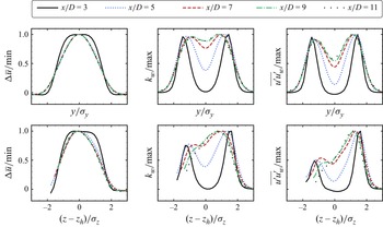
 Δu¯
Δu¯ kw
kw u′u′¯w


 x=−3D
x=−3D
 τ~k
τ~k
 x
x k−(τ)
k−(τ) k−(τ)
k−(τ)
 k−(τ)
k−(τ) k−(l)
k−(l)
 Ak,wa
Ak,wa Ak,wb
Ak,wb
 bk
bk
 k−(τ)
k−(τ) k−(τ)
k−(τ) νt=aνtνt,∞
 lm
lm δ=5D
δ=5D lm,∞max=0.35δ
 Zk,w
Zk,w γk
γk
 x
x
 k−(τ)
k−(τ)
 u′u′¯
u′u′¯

 Zu′u′,w
 γu′u′
γu′u′
 x
x

 Iu,add
 u′u′¯
u′u′¯
 u′u′¯/u¯h
 u′u′¯
u′u′¯


 l
l τk
τk
 l
l τk
τk
 Open access

