


Impact Statement
This article discusses the importance and accessibility of accurate and timely sea state forecasts. It serves as a guide for a wider audience that might be interested in improving the accuracy of the local area forecasts.
1. Introduction
According to the United Nations Statistics Division, around 600 million people live in coastal areas that are less than 10 m above sea level, while nearly 2.4 billion people (about 40 per cent of the world’s population) live within 100 km of the coast (United Nations, 2017). Such proximity to the ocean has a great impact on the livelihood of the people—the coastal communities depend on the sea in many aspects, from transportation to sustenance. Providing great benefits, such proximity to the ocean brings great challenges as well. All the activities and general safety highly depend on the state of the ocean, and the ability to forecast the sea state accurately is of paramount importance.
Weather and sea state forecasting has been a subject of interest for more than a century. It is becoming more interesting with the latest extreme weather events brought by changes in the climate (Monirul Qader Mirza, Reference Monirul Qader Mirza2003). One has to be mindful of how difficult it is to produce accurate weather and sea state forecasts. There are numerous groups of professionals who work daily on forecasting models to produce accurate forecasts. The number of variables that one needs to account for, the computational expenses, the in-situ measurements, and satellite observations illustrate the huge amount of work that is required to produce an accurate forecast. High-standard models include the Global Forecast System (GFS), a weather forecast model produced by the National Centers for Environmental Prediction (NCEP); Wavewatch III (WW3) (wind and wave forecast), developed by an international team around NOAA/NCEP and used to forecast marine meteorology by Météo-France (for wave and submersion vigilance), SHOM, NOAA, and Previmer; the Wave Model (WAM); Icosahedral Nonhydrostatic Model (ICON).
In addition to just producing accurate forecasts, forecast validation and improvement have been long-standing questions. Brier and Allen (Reference Brier, Allen and Malone1951) talk about weather forecast validation being a controversial subject for the last 6 years, and the paper was published in 1951! So it is clear that the question “How good is a certain forecast?” has been out there from the beginning of forecasting.
When talking about forecast evaluation, we need to specify precisely what we are trying to achieve and what the purpose of the verification is. Are we pursuing an economic purpose, for example providing better meteorological and sea state forecasts for the fishermen of the Aran Islands, Ireland, or is our purpose purely scientific? Are we just interested in the individual model’s accuracy? In this article, we will present the results of a novel procedure for improving local sea state forecasts by utilizing observations from a low-cost buoy (Raghukumar et al., Reference Raghukumar, Chang, Spada, Jones, Janssen and Gans2019) and the free open-source ensembleBMA software (Fraley et al., Reference Fraley, Raftery, Gneiting and Sloughter2008).
An extensive research project in improving forecast errors and uncertainty was undertaken by the UW Probcast Group, resulting in a number of publications. The goals of the UW Probcast Group were to develop methods for evaluating the uncertainty of mesoscale meteorological model predictions, and to create methods for the integration and visualization of multi-source information derived from model output, observations, and expert knowledge; see Grimit and Mass (Reference Grimit and Mass2002) for example. A number of questions were addressed by the group, including the uncertainty in forecasts (Gneiting et al., Reference Gneiting, Raftery, Westveld and Goldman2005), calibration of forecasts ensembles, model evaluation (Fuentes and Raftery, Reference Fuentes and Raftery2005), and the work of Gneiting and Raftery (Reference Gneiting and Raftery2007) on proper forecast scoring rules, amongst many other publications.
The work presented in this article was inspired by the work of the UW Probcast Group. However, the original work of the UW Probcast Group focused on atmospheric variables, such as temperature, precipitation, and wind. The work presented in this publication concentrates on improving the sea state forecast. We will use the significant wave height (‘ $ {H}_s $
’) as a forecast variable that will be improved using the proposed techniques.
$ {H}_s $
’) as a forecast variable that will be improved using the proposed techniques.
Here we will present partial results of the ongoing project Wave Obs, which is part of the HIGHWAVE project. HIGHWAVE is an interdisciplinary European Research Council (ERC) project at the frontiers of coastal/ocean engineering, earth system science, statistics, and fluid mechanics that explores fundamental open questions in wave breaking. The objectives of the project are primarily to develop an innovative approach to include accurate wave breaking physics into coupled sea state and ocean weather forecasting models, but also to obtain improved criteria for the design of ships and coastal/offshore infrastructure, to quantify erosion by powerful breaking waves, and finally to develop new concepts in wave measurement with improved characterization of wave breaking using real-time instrumentation. The project includes new approaches to field measurements and breaking wave forecast improvements. The Wave Obs project develops tools for improved wave forecasts, but at the same time plays a role in the whole project by providing daily forecasts for the team, and a wider audience.
Wave Obs started in January 2020 as an alert service for the project engineer. This alert service was put in place for timely weather warnings and to assist in the planning of instrument deployment and maintenance. As mentioned above, HIGHWAVE is an interdisciplinary project that requires extensive instrument deployment and real-time data transmission. The physical research station is currently located on Inis Meáin, Aran Islands, a place of highly energetic wave events, strong gale force winds, and rapidly changing weather. Hence weather and sea state dependence is a high risk factor for the successful completion of all aims of HIGHWAVE, which requires careful planning.
The original aim of Wave Obs was to provide daily forecasts from various sources to allow for accurate planning of instrument deployment and maintenance. Wave Obs has developed further, and now comprises a collection of historical daily forecasts that are stored on the HIGHWAVE website (www.highwave-project.eu) for the benefit of the team, and local community of the Aran Islands. Additionally, a Telegram bot has been set up, and the same daily forecasts are distributed through Telegram, where any member of the public can subscribe to receive daily forecasts, including a short text description and three plots with atmospheric and sea state variables. Constant striving to improve the provided information has led the authors to the idea of improving the collected forecasts by using Bayesian Model Averaging (BMA) techniques and providing an improved forecast. A short description of Wave Obs can be found in the Methods section. A more detailed description of particular variables of interest ( $ {H}_s $
) can be found in the Methods section as well.
$ {H}_s $
) can be found in the Methods section as well.
The article is structured as follows: in the Methods section, we present Wave Obs, observational data collection using weather stations and low-cost buoys, a short overview of the free ensembleBMA software, and basic statistics. In the Results section, we present a comparison of raw observation data with the forecasts, and then a comparison of improved forecasts with real ocean observations. In the Discussion section, we share our views on the possibility of extending the improved forecasts to a global scale, and discuss possible extensions to the improved forecast.
2. Methods
2.1. Wave Obs
Originally Wave Obs started as a warning tool for the HIGHWAVE project engineer based on the West Coast of Ireland. As the wider HIGHWAVE project requires instrument deployment in the field, weather plays an important role in planning the deployment of instruments. Wave Obs has developed and evolved into an intricate collection of forecasts from various sources, and includes not only wind and wave forecasts but many more variables, such as temperature, atmospheric pressure, and solar radiation. Initially, Wave Obs was a manual task. On a daily basis, the forecasts for the next 3 days were collected from the different sources, then the forecasts were passed to the interested parties, and a database was populated manually. The forecast collection process was automated in May 2020. A Python application was developed to automatically download, process, and distribute the forecast data from the different sources. This application extracts a number of sea state and meteorological variables for several locations around the Aran Islands region (Figure 1), accessing the servers of the forecast data providers through different API protocols.
Locations (marked with red $ X $
) of the points where the forecasts are obtained for.
$ X $
) of the points where the forecasts are obtained for.

Considering that all data providers deliver their data in numerous kind of formats and specifications, a process of data cleaning and transformation into a uniform format is applied and then the data is stored locally using a JSON (JavaScript Object Notation) file format. Each file contains the forecast for five consecutive days, and it is stored following the name convention given by the current date. The automation process is carried out by GitHub workflows and includes two basic steps: first, data is stored in the Google Drive cloud servers on a daily basis, and second, using a Telegram bot, a daily digest on the marine weather forecast contrasting different sources is automatically sent to a Telegram channel, making it available for the Aran Islands local community (see Wave Obs pipeline in Figure 2).
Wave Obs pipeline showing a brief description of the data collection, processing, and distribution.

In the development of the project, it was established that many agencies that provide forecasts draw the actual information from just a handful of sources. Hence it was decided to only track “original” sources. As this article concentrates on wave forecasts and measurements, we list the wave information forecasts only.
2.1.1. Sources
As mentioned above, only four sources are considered for forecast collection. A brief description of each source is presented below.
-
• Marine Institute (Ireland): The numerical wave model, SWAN, simulates surface gravity waves for a domain covering Irish waters at a resolution of 0.025° (approximately 1.5 km). The model uses Global NCEP GFS for wind forcing and FNMOC WW3 data for the wave boundary conditions. A daily 6-day forecast is generated for wave parameters such as $ {H}_s $
, swell wave height, mean wave period, and mean wave direction. The Marine Institute provides its data through the THREDDS and ERDDAP protocols. The latter is used to access the data using the Wave Obs application. We will denote the Marine Institute as “MI” in the figures and tables that follow.
$ {H}_s $
, swell wave height, mean wave period, and mean wave direction. The Marine Institute provides its data through the THREDDS and ERDDAP protocols. The latter is used to access the data using the Wave Obs application. We will denote the Marine Institute as “MI” in the figures and tables that follow. -
• NOAA WAVEWATCH III Global: Well-established and widely used model with spatial resolution 0.25° and temporal resolution of 1 h. This is a global forecast issued by NOAA/NCEP. WAVEWATCH III, alike SWAN, solves the random phase spectral action density balance equation for wavenumber-direction spectra. The forecast data is officially delivered using an ERDDAP server. NOAA/NCEP WAVEWATCH III data is the most comprehensive forecast; it includes wind speed and direction, and main wave sea state parameters (wave height, mean period, and direction) for the three main spectral partitions (wind waves, and primary and secondary swells). We will denote NOAA WAVEWATCH III Global as “WW3” in the figures and tables that follow.
-
• Météo-France Wave Model (MFWAM) Global Forecast: The operational global ocean analysis and forecast system of Météo-France with a spatial resolution of 1/12° and a temporal resolution of 3 h provides daily analysis and 5-day forecast for the global ocean sea surface waves. Météo-France uses an implementation of the third-generation spectral wave model WAM (The Wamdi Group, 1988). This product includes 3-hourly instantaneous fields of integrated wave parameters from the total spectrum (
$ {H}_s $
, period, direction, Stokes drift, and others), as well as the following partitions: the wind wave, and the primary and secondary swell waves. We will denote the Météo-France Wave Model Global as “MF” in the figures and tables that follow. -
• DWD Wave Model Global: This forecast model, alike MF, uses the generation wave model WAM (The Wamdi Group, 1988). This forecast is issued by the German Weather Service (DWD). A global domain with spatial resolution of 0.25° and temporal resolution of 3 h is used. The wind forcing is obtained from the ICON modeling framework, which is a joint project between the German Weather Service and the Max Planck Institute for Meteorology. We will denote the DWD Wave Model Global as “DWD” in the figures and tables that follow.


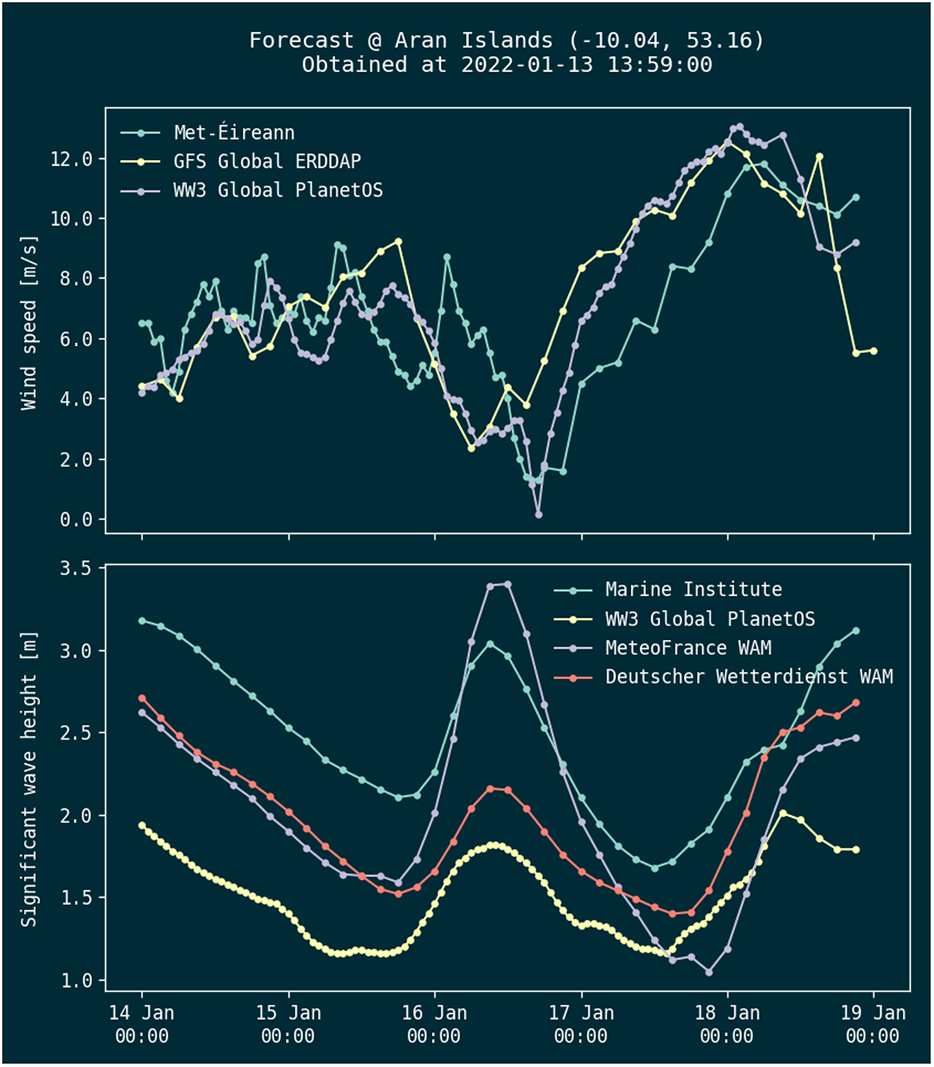
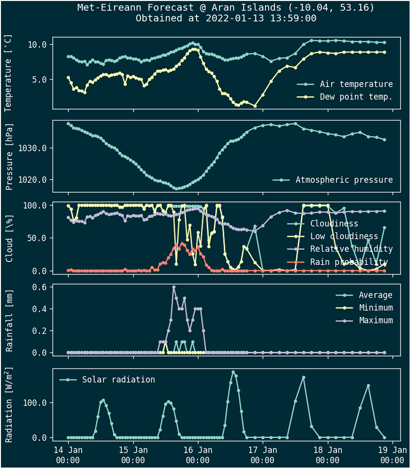
As HIGHWAVE experiments take place on the West Coast of Ireland, and the Mobile Research Station (MRS) is currently located on Inis Meáin, one of the Aran Islands, daily forecasts were made available to the local island community. This was achieved by posting 5-day forecasts daily on the HIGHWAVE website (see examples in Figures 3 and 4). The same forecasts are delivered through a Telegram channel to anyone who has subscribed to it. It is accompanied by a short text description of the weather and sea state expected in the next 5 days.
Wind and wave forecast example.
Atmospheric variables forecast.
In addition to the graphs, a database containing the daily forecasts collection has been developed. Data from this database will be used to validate and train the new and improved forecast.
2.2. Observational data collection
The main goal being an improvement of the forecasts in the future, it is desirable to validate the forecasts in order to determine the accuracy of the available forecasts. To achieve that, a weather station was installed for the validation of atmospheric variables. To establish the accuracy of the sea state forecast, two low-cost buoys were deployed in the area of interest. Since we are interested in the sea state forecast, we will only present the data collection process from the buoys and not from the weather station.
2.2.1. Buoys
As part of the HIGHWAVE project, two Spotter buoys were purchased. They were named Wanderer and Explorer. With these two buoys, three campaigns were completed:
-
• Wanderer first mission - June 1, 2020–September 19, 2020
-
• Explorer first mission - August 11, 2020–September 5, 2020
-
• Explorer first mission - adrift - September 5, 2020–October 1, 2020
-
• Wanderer second mission - November 7, 2020–March 3, 2021
The data of interest can be obtained by the software on board the buoys, either in real-time through satellite connection or directly from the SD card after recovery of the buoy. The downside of using the pre-processed data, in general, is that the on-board algorithms are a “black box” as such, and the end user is not aware of how the $ {H}_s $
, for example, is calculated. The following variables are recorded by the Spotter buoys:
$ {H}_s $
, for example, is calculated. The following variables are recorded by the Spotter buoys:
-
•
$ {H}_s $
, for all practical purposes:

 $$ {H}_s\approx 4\sqrt{m_0}, $$
where $ {m}_0 $
is the zeroth-order moment of the variance density spectrum
$ {m}_0 $
is the zeroth-order moment of the variance density spectrum $ E(f) $
. In the wave mode, the
$ E(f) $
. In the wave mode, the $ {H}_s $
is estimated from the zeroth-order moment of the wave spectrum (Sofar Ocean Technologies, 2022).
$ {H}_s $
is estimated from the zeroth-order moment of the wave spectrum (Sofar Ocean Technologies, 2022).
-
1. Mean Wave Period (
$ {\overline{T}}_0 $
) and Peak Wave Period (
$ {T}_p $
), where the mean period is the variance-weighted mean period (
$ {T}_{m_{01}} $
), and the Peak Period is the period associated with the peak of the wave spectrum. -
2. Mean (
$ \overline{\theta} $
) and Peak (
$ {\theta}_p $
) Directions: One can define the peak direction
$ {\theta}_p $
as the direction corresponding to the most energetic wave component. It is calculated in terms of the circular moments or Fourier coefficients
$ {a}_1(f) $
and
$ {b}_1(f) $
, which are the result of the cross-spectral analysis of the wave-induced horizontal wave displacement and surface elevation (
$ x $
,
$ y $
, and
$ z $
, respectively) as shown by Kuik et al. (Reference Kuik, van Vledder and Holthuijsen1988). The exact definitions of both peak wave direction and mean direction are


 $$ {\theta}_p={\tan}^{-1}\left\{\frac{b_1\left({f}_p\right)}{a_1\left({f}_p\right)}\right\}, $$
and
 $$ \overline{\theta}={\tan}^{-1}\left\{\frac{{\overline{b}}_1}{{\overline{a}}_1}\right\} $$
respectively, where the overbar indicates energy-weighted averaged quantities.
-
• Other wave parameters, including mean and peak directional spreading.
In this article, we only concentrate on $ {H}_s $
. The comparison between the Spotter-recorded data and forecasts from various agencies is presented in the Results section (Section 3).
$ {H}_s $
. The comparison between the Spotter-recorded data and forecasts from various agencies is presented in the Results section (Section 3).
2.3. Statistics
In order to evaluate the accuracy of the individual forecast and the “trained” ensemble forecast, we use the mean absolute error (MAE), mean absolute percentage error (MAPE) in some instances, and the continuous rank probability score (CRPS). In addition, individual weights of each forecast, contributing to the ensemble forecasts, were monitored, see Figure 9.
Let $ {y}_i $
be the observed value,
$ {y}_i $
be the observed value, $ {f}_i $
be a point forecast, and
$ {f}_i $
be a point forecast, and $ {F}_i $
be the probabilistic forecast for each observation
$ {F}_i $
be the probabilistic forecast for each observation $ i=1,2,\dots, n $
. MAE, MAPE, and CRPS can be calculated using the model forecasts and observations, as per equations (1)–(3), or using the built-in functions in the ensembleBMA software. These three measures were selected to evaluate the performance of individual, adjusted, and ensemble forecasts, as they are widely used in measuring the performance of probabilistic forecasts. In addition, MAE and CRPS were used to estimate the optimal training window for each buoy.
$ i=1,2,\dots, n $
. MAE, MAPE, and CRPS can be calculated using the model forecasts and observations, as per equations (1)–(3), or using the built-in functions in the ensembleBMA software. These three measures were selected to evaluate the performance of individual, adjusted, and ensemble forecasts, as they are widely used in measuring the performance of probabilistic forecasts. In addition, MAE and CRPS were used to estimate the optimal training window for each buoy.
The mean absolute error is given by
 $$ \hskip0.1em \mathrm{MAE}=\frac{\sum_{i=1}^n\mid {y}_i-{f}_i\mid }{n}. $$
The MAPE is similar to MAE, and is given by
 $$ \hskip0.1em \mathrm{MAPE}=\frac{1}{n}\sum \limits_{i=1}^n\frac{\mid {y}_i-{f}_i\mid }{\mid {y}_i\mid }. $$
The continuous rank probability score is widely used to assess the accuracy of probabilistic forecasts (e.g., Gneiting and Raftery, Reference Gneiting and Raftery2007). Let $ {F}_i $
be the cumulative distribution function of the probabilistic forecast for observation
$ {F}_i $
be the cumulative distribution function of the probabilistic forecast for observation $ i $
, then the continuous rank probability score is given as
$ i $
, then the continuous rank probability score is given as
 $$ \hskip0.1em \mathrm{crps}\hskip0.1em \left({F}_i,{y}_i\right)={\int}_{-\infty}^{\infty }{\left({F}_i(x)-H\left(x-{y}_i\right)\right)}^2 dx, $$
where $ H $
is the Heaviside step function. The mean CRPS is given as the average score over all instances:
$ H $
is the Heaviside step function. The mean CRPS is given as the average score over all instances:
 $$ \hskip0.1em \mathrm{CRPS}=\frac{1}{n}\sum \limits_{i=1}^n\hskip0.1em \mathrm{crps}\hskip0.1em \left({F}_i,{y}_i\right). $$
The value of the weight of the individual forecast indicates how much the individual model contributes to the ensemble forecast. By evaluating the weight of each individual contribution of forecast, it is possible to exclude forecasts that have no or little contribution to the ensemble. However, in the results presented here, we did not exclude low-weighting forecasts from the ensemble forecasts.
2.4. Bias-corrected forecasts
In the process of producing the ensemble-averaged forecast, individual forecast models are first bias-corrected (Gneiting et al., Reference Gneiting, Raftery, Westveld and Goldman2005, Sloughter et al., Reference Sloughter, Gneiting and Raftery2013). There are various ways of performing this process. We briefly describe how such a bias correction is completed in the ensembleBMA software.
Let $ {y}_i $
be the observed value, and let
$ {y}_i $
be the observed value, and let $ {f}_i $
be the point forecast for observation
$ {f}_i $
be the point forecast for observation $ i=1,2,\dots, n $
. A simple linear model is used to model the relationship between the forecast and the observed values. That is,
$ i=1,2,\dots, n $
. A simple linear model is used to model the relationship between the forecast and the observed values. That is,
 $$ {y}_i=a+b\hskip0.15em {f}_i+{\varepsilon}_i, $$
where $ {\varepsilon}_i\sim N\left(0,{\sigma}^2\right) $
. The linear model is fitted using least squares to yield parameter estimates
$ {\varepsilon}_i\sim N\left(0,{\sigma}^2\right) $
. The linear model is fitted using least squares to yield parameter estimates $ \hat{a} $
and
$ \hat{a} $
and $ \hat{b} $
. The bias-corrected forecasts are then given as
$ \hat{b} $
. The bias-corrected forecasts are then given as
 $$ {\hat{f}}_i=\hat{a}+\hat{b}\hskip0.15em {f}_i; $$
the estimates $ \hat{a} $
and
$ \hat{a} $
and $ \hat{b} $
determine how much the forecast needs to be shifted and scaled in the bias-correction process. Furthermore, the linear model gives a probabilistic individual forecast, where
$ \hat{b} $
determine how much the forecast needs to be shifted and scaled in the bias-correction process. Furthermore, the linear model gives a probabilistic individual forecast, where
 $$ {Y}_i\mid {f}_i\sim N\left(a+ b\hskip0.15em {f}_i,{\sigma}^2\right). $$
In practice, the bias-correction process is fitted to a time window of $ m $
observations and it is then applied to forecasts immediately after the time window.
$ m $
observations and it is then applied to forecasts immediately after the time window.
2.5. Bayesian Model Averaging techniques
The forecasting process used to be a deterministic one. It was believed that if you initialized your model with the most accurate input information, you would produce the most accurate forecast. However, with advances in high-performance computing and available resources, ensemble forecasts became available. An ensemble forecast is one that would consist of a number of numerical model outputs, with slightly perturbed initial conditions. For a comprehensive overview of ensemble forecasting, we refer the reader to Gneiting and Raftery (Reference Gneiting and Raftery2015). In essence, the ensemble forecasts are probabilistic ones, and even though both deterministic and probabilistic forecasting is trying to predict a certain “event,” the actual error or uncertainty can only be found in the probabilistic forecast. There are of course errors present in the ensemble forecasts as well. However, it has been shown by Gneiting et al. (Reference Gneiting, Raftery, Westveld and Goldman2005) that it is possible to improve the ensemble forecasts by applying some post-processing based on Bayesian Model Averaging techniques.
The essence of the BMA idea is in combining not the outcome of different initial conditions for one model but rather different models. Properly introduced in the late 1970s by Leamer (Reference Leamer1978), it did not get much attention till the 1990s (Kass and Raftery, Reference Kass and Raftery1995); see a comprehensive review in Hoeting et al. (Reference Hoeting, Madigan, Raftery and Volinsky1999), for example. We will not try to re-explain here the whole theoretical background for the BMA technique but will merely give the reader the basic idea.
The BMA forecasting model is based around taking a weighted combination of individual forecasting models. Suppose, we have $ K $
bias-corrected individual forecasting models (see Section 2.4), then the BMA forecast based on (4) is given as
$ K $
bias-corrected individual forecasting models (see Section 2.4), then the BMA forecast based on (4) is given as
 $$ {Y}_i\mid {f}_{1i},{f}_{2i},\dots, \hskip0.35em {f}_{Ki}\sim \sum \limits_{k=1}^K{w}_kN\left({a}_k+{b}_k\hskip0.35em {f}_{ki},{\sigma}^2\right). $$
The unknown parameters are estimated using an expectation–maximization (EM) algorithm (Dempster et al., Reference Dempster, Laird and Rubin1977), and the details of this are given in (Gneiting et al., Reference Gneiting, Raftery, Westveld and Goldman2005, Section 2b).
A point forecast of $ {Y}_i $
from the BMA model is thus given as
$ {Y}_i $
from the BMA model is thus given as
 $$ {\hat{y}}_i=E\left({Y}_i|\hskip0.35em ,{f}_{1i},\hskip0.35em ,{f}_{2i},\dots, \hskip0.35em ,{f}_{Ki}\right)=\sum \limits_{k=1}^K{w}_k\left({a}_k+{b}_k\hskip0.35em {f}_{ki}\right), $$
which is a weighted average of the bias-corrected individual forecasts. In practice, the weights are also estimated using an $ m $
observation time window and used for subsequent forecasts.
$ m $
observation time window and used for subsequent forecasts.
Thus, in BMA, rather than concentrating on the various outputs of one selected model, a number of different models are considered, determined by the estimated weights $ {\hat{w}}_1,{\hat{w}}_2,\dots, {\hat{w}}_K $
. As shown below (Section 3.3.1), it is possible, and it is the case, that one model outperforms another for a short period of forecasting, with the original model performing better again later. In the case of sea state forecast, it can be as simple as one model being better at predicting calm summer seas, and another being more accurate in the winter. We present below the evidence of one model outperforming another in different conditions.
$ {\hat{w}}_1,{\hat{w}}_2,\dots, {\hat{w}}_K $
. As shown below (Section 3.3.1), it is possible, and it is the case, that one model outperforms another for a short period of forecasting, with the original model performing better again later. In the case of sea state forecast, it can be as simple as one model being better at predicting calm summer seas, and another being more accurate in the winter. We present below the evidence of one model outperforming another in different conditions.
2.5.1. Data distribution normality assumption
The proposed method, as outlined in Sections 2.4 and 2.5, is based on a normality assumption for the difference between the adjusted forecast and the observed significant wave height (see equations (4) and (5)). The proposed BMA technique, based on the normality assumption, has also been successfully used in previous studies for sea-level air pressure and temperature forecasting (Raftery et al., Reference Raftery, Gneiting, Balabdaoui and Polakowski2005). However, there also exist BMA techniques based on non-normal distributions (Sloughter et al., Reference Sloughter, Raftery, Gneiting and Fraley2007) which have been successfully used for precipitation forecasts.
We investigated the use of using the BMA approach with other distributional assumptions (e.g., gamma distribution), but we found that the results were less accurate than the approach based on the normal distribution.
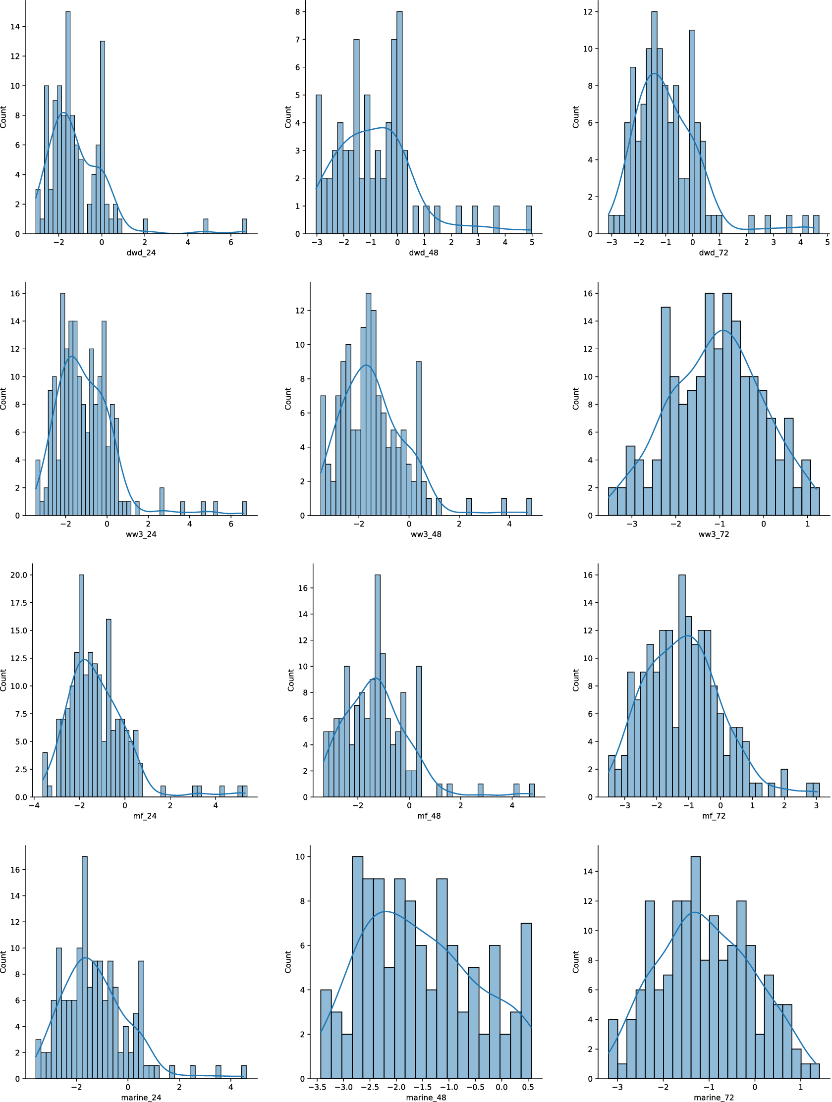
We investigated the normality assumption by comparing the observed significant wave height to the bias-adjusted forecasts using histograms and QQ-plots, see Figures 5 and 6 for the M6 winter adjusted forecasts (all other missions are provided in the Supplementary Material). The results showed that the normality assumption held approximately, but some extreme differences were observed that were not well accommodated by the normal distribution. This suggests that an extension of the proposed approach could be developed using heavy-tailed distributions to accommodate these large differences.
Histograms of the difference between the adjusted forecasts for M6 winter period versus the actual observed value. From top to bottom: DWD, WW3, MF, Marine Institute. From left to right: 24H, 48H, 72H.
Q-Q plots of the difference between the adjusted forecast for M6 winter period versus the actual observed value. From top to bottom: DWD, WW3, MF, Marine Institute, from left to right: 24H, 48H, 72H.

3. Results
3.1. Forecasts vs buoy observations
As mentioned in the Methods section, we present here a “brute force” comparison between the forecasts of interest and records from Spotter buoy campaigns. As part of Wave Obs, we have been collecting 3-day forecasts until December/January 2020, and 5-day forecasts since January 2021. However, in this article, we concentrate on 24, 48, and 72 h forecasts, denoted 24H, 48H, and 72H in the plots and tables. In Figure 7 we present the 24, 48, and 72 h forecasts and the real data from the Wanderer first mission. A similar comparison is presented for the first Explorer and second Wanderer missions in the Supplementary Material; see Figures 33 and 34.
Comparing actual recorded $ {H}_s $
to the 24 h (top), 48 h (middle), and 72 h (bottom) forecasts of the
$ {H}_s $
to the 24 h (top), 48 h (middle), and 72 h (bottom) forecasts of the $ {H}_s $
for the first Wanderer mission.
$ {H}_s $
for the first Wanderer mission.

As one would expect, the forecasts are quite reasonable, and predict the $ {H}_s $
quite well. However, the further away the forecast from the forecast date, the less accurate it is, which is not surprising. In Table 1 we present the MAE for individual models, depending on the forecast hour. As mentioned above, the MAE values confirm that the 24 h forecast is the most accurate one. We present results for all missions and all model forecasts.
$ {H}_s $
quite well. However, the further away the forecast from the forecast date, the less accurate it is, which is not surprising. In Table 1 we present the MAE for individual models, depending on the forecast hour. As mentioned above, the MAE values confirm that the 24 h forecast is the most accurate one. We present results for all missions and all model forecasts.
Average mean absolute error (in meters) of individual forecasting models, depending on the forecast time for Explorer I, Wanderer I, and Wanderer II missions

Note: The graphs reflecting the difference between the first Explorer and second Wanderer missions are provided in the Supplementary Material.
a Note the improved accuracy of either 48H or 72H forecasts.
b Note the accuracy of the 72H matching the 24H accuracy.
We would like to point out that the previous statement regarding the accuracy of the forecast that decreases with a longer time lag is still true for the DWD. However, the WW3 and MF models do not follow the same behavior. Overall, for the period covered, the best accuracy shifts to either 48 h or even 72 h forecasts at some stage, or matches the accuracy of the 24 h forecast.
Similar results are presented in the Supplementary Materials, Figures 33 and 34 for the first Explorer and second Wanderer missions. The period covered is between June 2020 and early March 2021. This period, which included calm summer seas and rough winter seas, can be considered versatile enough for forecast training purposes. The interannual variability is a valid concern point that can be raised. The long-term variability of wave climate and extreme wave events, particularly at the Irish coast, North Atlantic, and the Bay of Biscay, have been a topic of a number of recent studies. However, an overall message is that for the period 1979–2012 at least there were no significant trends for the mean up to the 99th percentile of significant wave height, with the caveat that climate trends are very hard to differentiate from low frequency variability in the climate system. For the comprehensive review of studies regarding wave climate trends, we would refer the reader to Gallagher et al. (Reference Gallagher, Tiron and Dias2014) and Gallagher et al. (Reference Gallagher, Gleeson, Tiron, McGrath and Dias2016).
The total observational period with the Spotter buoys was between June 2020 and early March 2021, and for the M6 location, the authors looked at summer 21 June 2020–September 2020, and separately for October 20, 2021–November 20, 2021. The same process of forecast improvement was carried out for the period between June 2020 and March 2021 for the Spotter buoy in retrospect. In other words, we produced a daily ensemble forecast for this period, and compared it to the actual observations. Hence, we believe that seasonality was taken into consideration in the training process. These retrospect forecasts are not presented for the sake of brevity.
The months of April and May were not included, and hence the whole year was not covered. But this should not be an issue due to the training period selected. For the three missions (Explorer I, Wanderer I, and Wanderer II), the sliding training period was 5, 10, and 20 days, respectively. Even at the maximum training period of 20 days, the window is a sliding window, and hence the changing conditions are being captured by the training period, as the forecast develops in time.
As previously mentioned, the months of April and May have not been part of the forecast improvement period. Even though a number of unusual weather events tend to occur in Ireland during the month of April, on most occasions these events are heatwaves, or extreme rainfall events—but not marine heatwaves that would affect the whole oceanic ecosystem including wave heights.
Overall, we are confident, that since the training window is not fixed, and is of a sliding nature, any variability that might affect the forecast will be captured during the training period, as it moves together with the improved forecast. However, the subject of training windows will be addressed separately.
Taking into account the Explorer drifting period, and the period of change of the data collection algorithm, from here, we will only present the results of the first Wanderer mission. Results from the two other missions are available in the Supplementary Material.
Before any forecast training could begin, the optimal training window had to be established. Adopting the approach described in Raftery et al. (Reference Raftery, Gneiting, Balabdaoui and Polakowski2005), a sliding window of length $ m $
(number of days) was chosen.
$ m $
(number of days) was chosen.
To select the right value for $ m $
, a number of factors need to be considered. One would expect that the longer the training window, the better the training process would be. However, with longer periods, one might end up accumulating forecast errors for longer. In addition, the behavior of ocean waves is not as uniform as that of temperature. For example, one would expect temperatures to stay within average summer values during the months of June and July. Ocean waves, however, are known to have rapidly changing patterns, and for that reason, one would prefer to have a short training period—one capable of adapting quickly to changing conditions. During the selection process, authors looked at MAE and CRPS with a range of values for
$ m $
, a number of factors need to be considered. One would expect that the longer the training window, the better the training process would be. However, with longer periods, one might end up accumulating forecast errors for longer. In addition, the behavior of ocean waves is not as uniform as that of temperature. For example, one would expect temperatures to stay within average summer values during the months of June and July. Ocean waves, however, are known to have rapidly changing patterns, and for that reason, one would prefer to have a short training period—one capable of adapting quickly to changing conditions. During the selection process, authors looked at MAE and CRPS with a range of values for $ m $
from 5 to 90 days.
$ m $
from 5 to 90 days.
In Figure 8 we present the evolution of the MAE and CRPS, depending on the number of training days selected. Similar plots are presented in the Supplementary Material for the Explorer I and Wanderer II missions in figure 35. From Figure 8 it is clear that at some point extending the training window will no longer improve the accuracy: the values of MAE and CRPS plateau. Similar observations can be found in Gneiting et al. (Reference Gneiting, Raftery, Westveld and Goldman2005).
Comparison of first Wanderer mission training period lengths for $ {H}_s $
: MAE (top, meters), CRPS (bottom).
$ {H}_s $
: MAE (top, meters), CRPS (bottom).

Wanderer I weights of individual forecast models. It is clearly visible how MF is dominating the weight count towards the higher contribution to the ensemble forecast.

As can be seen from Figure 8, the lowest values of MAE and CRPS are at around 10 training days. Hence, a 10-day training window was selected for Wanderer’s first mission. The training window selection and MAE CRPS plots for Explorer I and Wanderer II missions are presented and discussed in the Supplementary Material, see Figure 35.
3.2. Ensemble forecast performance in coastal waters
In this section, the authors present the results of the improved forecast for the coastal areas. Explorer and Wanderer were deployed near Aran Islands, which can be considered to be in close proximity to the shore. In the next section, the results of the improved forecast in the open ocean are presented.
Once the training windows are selected, the training process is performed. The algorithm works as follows, using first the Wanderer mission as an example. We take forecasts and actual recorded data from the Spotter buoy from June 19, 2020, to June 29, 2020, and predict the significant wave height for June 30, 2020. Then we move to the time period from June 20 to June 30 and predict the $ {H}_s $
for July 1, 2020, and keep going until the end of the Wanderer’s first mission on September 18, 2020. During this process we track individual weights of each forecasting model (each broken down into three: 24H, 48H, and 72H, which results in 9 forecasts), and the overall CRPS and MAE. This process is two-fold: first we can see which individual forecasting model contributes the most to the ensemble forecast, and hence is more accurate in this instance; and we see the overall accuracy of the ensemble improved forecast. The evolution of individual weights is presented in Figure 37 in the Supplementary Material. In similar fashion, as before, the results of individual weights for Explorer I and Wanderer II are presented in the Supplementary Material in Figure 37.
$ {H}_s $
for July 1, 2020, and keep going until the end of the Wanderer’s first mission on September 18, 2020. During this process we track individual weights of each forecasting model (each broken down into three: 24H, 48H, and 72H, which results in 9 forecasts), and the overall CRPS and MAE. This process is two-fold: first we can see which individual forecasting model contributes the most to the ensemble forecast, and hence is more accurate in this instance; and we see the overall accuracy of the ensemble improved forecast. The evolution of individual weights is presented in Figure 37 in the Supplementary Material. In similar fashion, as before, the results of individual weights for Explorer I and Wanderer II are presented in the Supplementary Material in Figure 37.
In addition, the authors looked at the number of effective forecasts over time. This value of entropy shows the number of effective forecasts used in the production of the ensemble forecast. The results of the Wanderer I mission are presented in Figure 10. The same information for the Explorer I and Wanderer II missions is presented in the Supplementary Material in Figure 38.
Wanderer I number of effective forecasts over time.

One of the main reasons why the authors looked at the number of effective forecasts was to understand if the ensemble forecast is only dominated by one model at a time. From Figure 10 it can be seen that there are 6 days where the ensemble forecast is dominated by one forecast model. However, this represents only 7.4 $ \% $
of the total time period. For
$ \% $
of the total time period. For $ 45.7\% $
of the time, the number of effective forecasts is two, and for
$ 45.7\% $
of the time, the number of effective forecasts is two, and for $ 24.7\% $
of the time, it is three. Four effective forecasts are present in the ensemble for
$ 24.7\% $
of the time, it is three. Four effective forecasts are present in the ensemble for $ 14.8\% $
of the time, and we can see that five forecasts are effective for
$ 14.8\% $
of the time, and we can see that five forecasts are effective for $ 7.4\% $
of the time.
$ 7.4\% $
of the time.
3.3. Ensemble forecast performance in the open ocean
The results mentioned in the previous section were obtained by using the historical collected forecasts and not the real-time data from the Spotter buoys. A natural question arises: can the approach be extended to real-time forecasting? In this section, the authors will present the results of applying the process to the real-time forecast for the M6 buoy location, off the West Coast of Ireland, for the period of October 2, 2021 to October 20, 2021. The period of the summer of 2020 was used as a training and validation example as well.
M6 is a part of the Irish Marine Weather Buoy Network. It is a joint project designed to improve weather forecasts and safety at sea around Ireland. The project is the result of collaboration between the Marine Institute, Met Éireann, The UK Met Office, and the Irish Department of Transport. Data from the M6 is publicly available through the Marine Institute and Met Éireann websites, with hourly updates. M6 is located at $ 53.07 $
N,
$ 53.07 $
N, $ -15.88 $
E, approximately
$ -15.88 $
E, approximately $ 210 $
nautical miles (
$ 210 $
nautical miles ( $ 389 $
km) west southwest of Slyne Head. In addition to atmospheric variables, oceanographic data, such as
$ 389 $
km) west southwest of Slyne Head. In addition to atmospheric variables, oceanographic data, such as $ {H}_s $
, wave period, maximum wave height, maximum wave period, mean direction, sea temperature, and salinity are recorded and made available to the public.
$ {H}_s $
, wave period, maximum wave height, maximum wave period, mean direction, sea temperature, and salinity are recorded and made available to the public.
For the purpose of this exercise, the data from M6 was collected on a daily basis, and the forecasts were collected as a daily routine for the Wave Obs project. Once the forecasts were collected, training was performed, and the new HIGHWAVE forecasts for the location were produced. The actual $ {H}_s $
on the following date is then compared to individual forecast models and the new ensemble HIGHWAVE forecast.
$ {H}_s $
on the following date is then compared to individual forecast models and the new ensemble HIGHWAVE forecast.
As described in the previous sections, the question of the optimal training window length $ m $
was addressed before any training and ensemble forecast production was performed. To achieve this, the time period between June 2020 to September 2020 was selected. This time period is the same as the time period covered by the Explorer first mission and Wandered first mission. Looking at straightforward forecast versus M6 measurements, we see a good agreement between the two, with the expected behavior of 24H forecast being more accurate than 48H or 72H (see Figure 11 [summer/autumn], and 12 [winter], and the values of MAE and MAPE in Table 2).
$ m $
was addressed before any training and ensemble forecast production was performed. To achieve this, the time period between June 2020 to September 2020 was selected. This time period is the same as the time period covered by the Explorer first mission and Wandered first mission. Looking at straightforward forecast versus M6 measurements, we see a good agreement between the two, with the expected behavior of 24H forecast being more accurate than 48H or 72H (see Figure 11 [summer/autumn], and 12 [winter], and the values of MAE and MAPE in Table 2).
M6 Met buoy area forecast from WW3, MF, and DWD for 24 h (top), 48 h (middle), and 72 h (bottom).

M6 Met buoy area forecast from WW3, MF, MI, and DWD for 24 h (top), 48 h (middle), and 72 h (bottom), for the winter period.

Mean absolute error (winter, m) and mean absolute percentage error (summer, $ \% $
) of individual raw forecasting models, depending on the forecast time for M6
$ \% $
) of individual raw forecasting models, depending on the forecast time for M6

Table 4 presents the mean absolute percentage error of individual forecasting models for the original forecasts (left columns) and bias-corrected forecasts (right columns). The MAPE of the HIGHWAVE forecast was equal to $ 0.12 $
. Comparing this value to the individual models, note the reduction in error can be as significant as
$ 0.12 $
. Comparing this value to the individual models, note the reduction in error can be as significant as $ 48\% $
. And the forecast improvement can be as high as
$ 48\% $
. And the forecast improvement can be as high as $ 8\% $
.
$ 8\% $
.
We would like to point out two observations one can make from this comparison. First, the values of MAE are lower for this location, compared to MAE values for the forecast near the Aran Islands. This is a direct confirmation that the forecast models considered are much better at predicting sea state in the open ocean (recall the M6 location). However, forecast accuracy starts to decrease as we get closer to the shore.
The selection of the sliding training window is based on the values of CRPS and MAE, as it was previously for the Spotter buoy missions. The training for a specific date was performed using 5, 10, 15, 20, to 85 training days at a time, for two different periods, summer and winter (Figure 13). It appears that 20 training days is a reasonable training period. From Figure 13 one can notice that 50 days seem even better—however, the authors opted for a shorter training period, due to the reasons mentioned before. One can notice the increase in the error in the winter period, similar to the Explorer I mission. This will be addressed further in the publication.
Selection of the training window for the M6 ensemble forecast during the summer period (top) and the winter period (bottom). MAE in meters.

Before live training and production of the ensemble forecast began, the suggested approach was tested on the aforementioned summer and winter periods. Using a range of training windows between 5 and 95 days, the overall values of MAE and CRPS were calculated for the ensemble forecasts, see Figure 13. In the summer period, both MAE and CRPS decrease with increasing training day period, as it was seen before in the Wanderer I mission. The winter period, however, displays a behavior where the error is increasing with increasing training window—this will be discussed separately. Looking at individual forecast model weights contributing most to the ensemble forecast, one can note that the MF and WW3 forecasts had dominant weights across the two periods, see Figure 14. We will address the question of weights of the individual models later. It is obvious that the ensemble forecast is more accurate than the raw un-adjusted individual forecast models. However, an additional question was asked: would individual bias-corrected model perform better than the ensemble forecast? As discussed in the Statistics section, as part of the ensembleBMA software, correction coefficients for each individual model can be obtained, see Figure 16. In the next section we present individual adjusted forecasts compared to the ensemble forecast. Values for the MAE and MAPE are presented in Tables 2 for the raw and 3 adjusted forecasts.
Weights of individual un-adjusted forecast models for the summer period (top) of 2020 and winter (bottom), at M6 buoy location.

Mean absolute error (winter, m) and mean absolute percentage error (summer, $ \% $
) of individual adjusted forecasting models, depending on the forecast time for M6
$ \% $
) of individual adjusted forecasting models, depending on the forecast time for M6

Similar to the Wanderer I, the authors looked at the effective number of forecasts for both periods at the M6 buoy. The results are presented in Figure 15.
Number of effective forecasts for M6 summer (top) and winter (bottom) period.

Bias coefficients for the corrected forecasts: intercept (a) top panel, slope (b) bottom panel.

3.3.1. Individual bias-corrected forecast performance versus the ensemble forecast
In this subsection, the authors compare the performance of the combined ensemble forecast (denoted HIGHWAVE) to individual bias-corrected models. As described above, this was “live” daily training between October 2, 2021, and October 20, 2021. It was performed with free ensembleBMA software and publicly available forecasts from each model mentioned here and below. The training was performed on an Intel(R) Core(TM) i7-4710HQ CPU @ 2.50GHz 2.49 GHz processor, with 16.0 GB RAM, and took seconds. There was no additional time spent on the forecast data collection, as it is a part of the automated process of Wave Obs.
In Figures 17 and 18 one can see that the adjusted MAPE or MAE in the case of winter period is lower on particular days, than the MAPE or MAE of the ensemble forecast. However, overall, over the whole period, HIGHWAVE ensemble forecast is on average more accurate than any raw or adjusted individual models.
Daily MAPE ( $ \% $
) of individual DWD—raw,– adjusted, and HIGHWAVE (top panel); MF—raw, – adjusted, and HIGHWAVE (middle panel); WW3—raw, – adjusted, and HIGHWAVE (bottom panel) forecasts for the summer period in the M6 location.
$ \% $
) of individual DWD—raw,– adjusted, and HIGHWAVE (top panel); MF—raw, – adjusted, and HIGHWAVE (middle panel); WW3—raw, – adjusted, and HIGHWAVE (bottom panel) forecasts for the summer period in the M6 location.
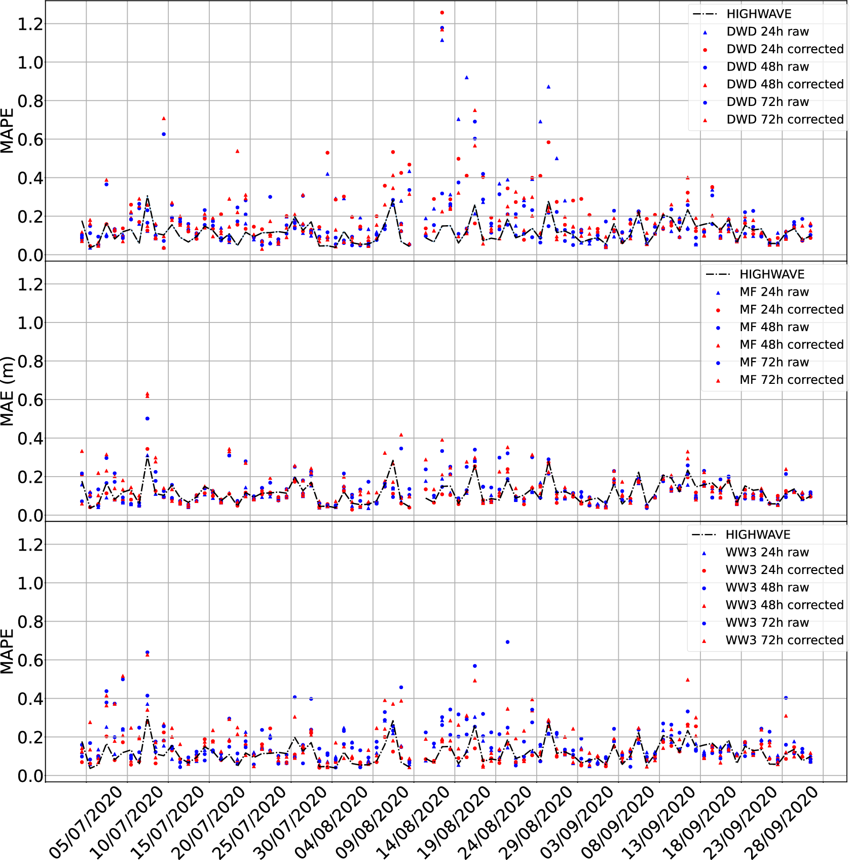
Daily MAE of individual DWD—raw,- adjusted, and HIGHWAVE (top panel); MF—raw, – adjusted, and HIGHWAVE (second panel); WW3—raw, – adjusted, and HIGHWAVE (third panel); MI—raw, – adjusted forecasts for the winter period in the M6 location.

On average, over a month, taking into consideration all four models, the ensemble forecast produced, using the BMA techniques is at least $ \approx 1\% $
better than individual forecasting models, and
$ \approx 1\% $
better than individual forecasting models, and $ 3\% $
better on average. On a few days individual forecast models performed better than the ensemble forecast. However, this number is negligible, and this is reflected in the overall MAE values. The visual comparison of the HIGHWAVE ensemble forecast to the M6 buoy observation is presented in Figure 19.
$ 3\% $
better on average. On a few days individual forecast models performed better than the ensemble forecast. However, this number is negligible, and this is reflected in the overall MAE values. The visual comparison of the HIGHWAVE ensemble forecast to the M6 buoy observation is presented in Figure 19.
Ensemble forecasts (HIGHWAVE) produced by the procedure proposed in this publication compared to the actual record from the M6 buoy for the winter period.

In addition, from this set of data, it is clear that MF (24H) has the highest weight $ 45\% $
of the time, followed by WW3 (24H)
$ 45\% $
of the time, followed by WW3 (24H) $ 28\% $
, and DWD (24H)
$ 28\% $
, and DWD (24H) $ 10\% $
of the time. Figure 20 visualizes the contribution of each individual model in the ensemble forecast for the summer period.
$ 10\% $
of the time. Figure 20 visualizes the contribution of each individual model in the ensemble forecast for the summer period.
Visual representation of each individual model having the highest weight on the ensemble forecasts for the period of interest.

For the winter period, it is surprising to see that the 72H forecast has the dominant effect on the contribution towards the ensemble forecast (Figure 21).
Visual representation of each individual model having the highest weight on the ensemble forecasts for the winter period.

There is no particular pattern, as the forecast having the highest impact does change. There would be a week or two where for example one is dominating. For example, from June 30, 2020, till July 7, 2020, DWD 24H forecast has the highest weight. But then it can change to MF taking over for a week. The reasons behind that could be an extension to the present work.
4. Discussion and concluding remarks
The results of the present study indicate that it is possible to produce an averaged forecast for a particular location, with an accuracy at least $ \approx 1\% $
higher than any available model discussed in this work. The accuracy can be further improved upon by selecting a suitable training window, and possibly adjusting the weights of individual models, depending on the time of year, as we saw that different models perform better under different conditions. The
$ \approx 1\% $
higher than any available model discussed in this work. The accuracy can be further improved upon by selecting a suitable training window, and possibly adjusting the weights of individual models, depending on the time of year, as we saw that different models perform better under different conditions. The $ 1\% $
improvement might not seem like a lot at first sight. However, this is still an improvement, and it should be noted that it is “at least
$ 1\% $
improvement might not seem like a lot at first sight. However, this is still an improvement, and it should be noted that it is “at least $ 1\% $
.” In reality, we are looking at improvement of the forecast up to
$ 1\% $
.” In reality, we are looking at improvement of the forecast up to $ 8\% $
. If we were to look at the reduction of error, in the M6 case presented in the article, we see the range of the mean absolute percentage error reduction between
$ 8\% $
. If we were to look at the reduction of error, in the M6 case presented in the article, we see the range of the mean absolute percentage error reduction between $ 1-9\% $
, see Table 4, with HIGHWAVE forecast yielding a
$ 1-9\% $
, see Table 4, with HIGHWAVE forecast yielding a $ 0.12 $
value for the MAPE. In the case of forecast improvement for the M6 winter period, we see the error reduction between the minimum of
$ 0.12 $
value for the MAPE. In the case of forecast improvement for the M6 winter period, we see the error reduction between the minimum of $ 6\% $
to substantial
$ 6\% $
to substantial $ 48\% $
. This is comparable with other attempts at wave forecast improvement, see for example Callens et al. (Reference Callens, Morichon, Abadie, Delpey and Liquet2020), where random forest and gradient boosting trees were used to improve wave forecast at a specific location, and the authors achieved a
$ 48\% $
. This is comparable with other attempts at wave forecast improvement, see for example Callens et al. (Reference Callens, Morichon, Abadie, Delpey and Liquet2020), where random forest and gradient boosting trees were used to improve wave forecast at a specific location, and the authors achieved a $ 39.8\% $
error decrease in their proposed method, which is comparable with our range of
$ 39.8\% $
error decrease in their proposed method, which is comparable with our range of $ 6-48\% $
. Other attempts, mostly involving Machine Learning and Neural Networks have been a highlight in recent years, see for example Londhe et al. (Reference Londhe, Shah, Dixit, Balakrishnan Nair, Sirisha and Jain2016) for a coupled numerical and artificial neural network model for improving location-specific wave forecast. In similar fashion the tidal predictions were addressed, see for example Yin et al. (Reference Yin, Zou and Xu2013).
$ 6-48\% $
. Other attempts, mostly involving Machine Learning and Neural Networks have been a highlight in recent years, see for example Londhe et al. (Reference Londhe, Shah, Dixit, Balakrishnan Nair, Sirisha and Jain2016) for a coupled numerical and artificial neural network model for improving location-specific wave forecast. In similar fashion the tidal predictions were addressed, see for example Yin et al. (Reference Yin, Zou and Xu2013).
Mean absolute percentage error of individual forecasting models, depending on the forecast time for M6 summer period ( $ \% $
)
$ \% $
)

We believe that it is a good improvement, since the shores on the West Coast of Ireland experience waves reaching very steep values during winter storms (O’Brien et al., Reference O’Brien, Dudley and Dias2013; O’Brien et al., Reference O’Brien, Renzi, Dudley, Clancy and Dias2018). It is not computationally expensive, and can be completed without the use of cluster or any type of high-performance computing. Implementing the forecast collection process is straightforward. It only requires the Wave Obs package, available on GitHub. EnsembleBMA software used for training of the forecasts is free software available from cran.r-project.org. This free access to information and the straightforward process of collecting and training the forecast opens up the opportunity to a wider population to use this tool for their daily needs. This might appeal to harbour-masters, fisherman, and others who depend on an accurate sea state forecast. Of course, the authors are aware of recent works in the forecast improvement area with Machine Learning algorithms (Guillou and Chapalain, Reference Guillou and Chapalain2021, Gracia et al., Reference Gracia, Olivito, Resano, Martin-del-Brio, de Alfonso and Álvarez2021, amongst many others). Readers interested in Machine Learning algorithms are referred to Ali et al. (Reference Ali, Fathall, Salah, Bekhit and Eldesouky2021) for evaluation of Machine Learning, Deep Learning, and Statistical Predictive Models. However, the nature of ML requires specific knowledge and training to perform such improvements. For example in Wu et al. (Reference Wu, Stefanakos and Gao2020), the PBML model has an MAE of $ 0.1961 $
for 24 h lead time forecast of the
$ 0.1961 $
for 24 h lead time forecast of the $ {H}_s $
, to be compared with the HIGHWAVE MAE of
$ {H}_s $
, to be compared with the HIGHWAVE MAE of $ \approx 0.08 $
for the 24 h forecast. In no way the authors are trying to downshift the role of ML algorithms in improving the sea state forecasting. However, one can consider different applications of ML and Wave Obs. Where ML can be used on large scale predictions, it might be beneficial, on a local scale, in terms of how easy it is to use, and the low computational cost of the Wave Obs process to be considered as a possibility for a non-scientific community audience.
$ \approx 0.08 $
for the 24 h forecast. In no way the authors are trying to downshift the role of ML algorithms in improving the sea state forecasting. However, one can consider different applications of ML and Wave Obs. Where ML can be used on large scale predictions, it might be beneficial, on a local scale, in terms of how easy it is to use, and the low computational cost of the Wave Obs process to be considered as a possibility for a non-scientific community audience.
The only issue is the availability of real-time or even historical data for the purposes of training. If there are some buoys in the area of interest and the data is publicly available, one can produce improved ensemble forecasts using the combination of the recorded measurements and available forecasts. However, if there is no field data available, the training process would suffer from the lack of data.
We investigated the possibility of extending this improved forecast to all coastal areas around Ireland. It was found that there exist 11 buoys that have live data available to the public that can be used in the training process. However, the distribution of the buoys would not allow for cross-coverage of the whole coastal area, please refer to Figure 22 to see the locations, and the extent of the forecast resolution around each buoy.
Map of buoys with open-access data around Ireland.

Despite the issues in extending the improved ensemble forecast to a global scale, it can be concluded that if a particular area requires more accurate forecasting (due to fishing, sailing, or transportation activities), it can easily be achieved using the approach described in this publication.
Abbreviations
- API API
-
Application Programming Interface
- BMA
-
Bayesian Model Averaging
- CDF
-
Cumulative Distribution Function
- CPU
-
Central Processing Unit
- CRPS
-
Continuous Rank Probability Score
- DWD
-
Deutscher Wetterdienst (German weather forecasting service)
- ERC
-
European Research Council
- ERDDAP
-
Environmental Research Division’s Data Access Program
- FNMOC
-
Fleet Numerical Meteorology and Oceanography Center
- GFS
-
Global Forecast System
- ICON
-
Icosahedral Nonhydrostatic Model
- JSON
-
JavaScript Object Notation
- MAE
-
Mean Absolute Error
- MAPE
-
Mean Absolute Percentage Error
- MF
-
Météo-France
- MI
-
Marine Institute
- ML
-
Machine Learning
- MRS
-
Mobile Research Station
- NCEP
-
National Centers for Environmental Prediction
- NOAA
-
National Oceanic and Atmospheric Administration
- RAM
-
Random-access memory
- SHOM
-
Service Hydrographique et Océanographique de la Marine
- SWAN
-
Simulating WAves Nearshore
- THREDDS
-
Thematic Real-time Environmental Distributed Data Services
- UW
-
University of Washington
- WAM
-
the Wave Model
- WW3
-
Wavewatch III
Acknowledgments
We acknowledge Arnaud Disant for the idea of the alert service, the Wave Group members who contributed to the daily collection and publishing of the forecasts, the Aran Island community for providing eyewitness evidence of some events, and the reviewers for their valuable and thoughtful comments and efforts toward improving our manuscript.
Author contribution
Conceptualization: B.M.; F.D. Methodology: B.M; T.K.; D.S. Data curation: F.D. Data visualization: T.K. Writing original draft: T.K; D.S.; F.D.; B.M. All authors approved the final submitted draft.
Competing interest
The authors declare no competing interests exist.
Data availability statement
Wave Obs toolkit is not publicly accessible at present, but the authors will share it upon request through GitHub repository. ensembleBMA software is available through ensembleBMA. Forecast data has been obtained from PlanetOS API, Met Éireann data interface, and the ERDDAP servers of NOAA/NCEPCoastWatch, Pacific Islands Ocean Observing System (PacIOOS) and Irish Marine Institute. Likewise, M6 data can be freely obtained from Marine Institute website. Historical forecasts for the Aran Island area are available upon HIGHWAVE.
Ethical standard
The research meets all ethical guidelines, including adherence to the legal requirements of the study country.
Funding statement
This work was supported by the European Research Council (ERC) under the research project ERC-2018-AdG 833,125 HIGHWAVE; Science Foundation Ireland (SFI) under Grant number SFI/12/RC/2289-P2; and Science Foundation Ireland (SFI) under Marine Renewable Energy Ireland (MaREI), the SFI Centre for Marine Renewable Energy Research (grant 12/RC/2302).
Supplementary material
The supplementary material for this article can be found at http://doi.org/10.1017/eds.2023.31.


 Open access

