


1. Introduction
Type One Energy is pursuing the high field approach to stellarator fusion energy. Plasma confinement in toroidal magnetic confinement devices like stellarators is governed by perpendicular collisional (neoclassical) and turbulent transport. These processes scale with the ratio of ion gyroradius, $\rho _i = (m_i T_i)^{0.5}/(Z_i eB)$
, to the minor radius
$\rho _i = (m_i T_i)^{0.5}/(Z_i eB)$
, to the minor radius $a$
, as quantified by
$a$
, as quantified by $\rho _* = \rho _i/a \sim 1/({B \cdot a})$
. Therefore, using strong magnetic fields provides an opportunity to achieve sufficient energy confinement for fusion power gain at smaller size.
$\rho _* = \rho _i/a \sim 1/({B \cdot a})$
. Therefore, using strong magnetic fields provides an opportunity to achieve sufficient energy confinement for fusion power gain at smaller size.
Many requirements related to thermal transport must be satisfied simultaneously to enable a stellarator fusion power plant. The energy confinement time $\tau _E$
and triple product
$\tau _E$
and triple product $n T \tau _E$
must be large enough to ensure large power gain with temperatures
$n T \tau _E$
must be large enough to ensure large power gain with temperatures $T \geqslant 10$
keV to maximize deuterium–tritium fusion reactivity, which sets limits on the allowable level of neoclassical and turbulent heat transport. Sufficient fuelling and particle transport characteristics are required to sustain the desired density while avoiding excessive accumulation of helium ash. A significant level of edge radiation is desired to support an exhaust management solution while avoiding untenable levels of core impurity accumulation. It must also be possible to access and sustain fusion burn within transport related density and beta limits using relevant actuator technology.
$T \geqslant 10$
keV to maximize deuterium–tritium fusion reactivity, which sets limits on the allowable level of neoclassical and turbulent heat transport. Sufficient fuelling and particle transport characteristics are required to sustain the desired density while avoiding excessive accumulation of helium ash. A significant level of edge radiation is desired to support an exhaust management solution while avoiding untenable levels of core impurity accumulation. It must also be possible to access and sustain fusion burn within transport related density and beta limits using relevant actuator technology.
Considerable progress has been made in understanding and predicting transport characteristics in stellarators through decades of observation and simulation. We review key results in § 2, from which it is possible to design the core physics configuration to meet the above requirements without further significant scientific advances. Type One Energy is designing high field stellarator power plants based on this understanding. We summarize our general approach here, before describing the background and choices in more detail in §§ 2 and 3. Configurations are optimized to minimize low collisionality neoclassical transport to enable a high temperature core with the intent of avoiding hollow density profiles. A pellet-fuelled scenario is proposed to support a large edge density gradient expected to minimize ion temperature gradient (ITG) turbulence. Focusing on quasi-isodynamic (QI) configurations with maximum-J provides a path to further minimize large contributions from density-gradient-driven trapped-electron mode turbulence. Configurations are also targeted to avoid ideal ballooning mode and kinetic ballooning mode (KBM) onset in regions of assumed large pressure gradient, which would otherwise limit performance. We conservatively target operation at or below densities near known radiative limits given the lack of evidence for sustained elevated confinement at more aggressive values. We are targeting high field, low $\beta$
scenarios that enable burning plasma conditions at relatively high density and low temperature while avoiding very narrow edge transport barriers. These conditions provide the best opportunity to access deeper pellet penetration to fuel and sustain elevated edge density gradients. These conditions should also provide large edge turbulent impurity transport to avoid core accumulation, enabling a large radiative fraction from an edge mantle as desired for heat exhaust management.
$\beta$
scenarios that enable burning plasma conditions at relatively high density and low temperature while avoiding very narrow edge transport barriers. These conditions provide the best opportunity to access deeper pellet penetration to fuel and sustain elevated edge density gradients. These conditions should also provide large edge turbulent impurity transport to avoid core accumulation, enabling a large radiative fraction from an edge mantle as desired for heat exhaust management.
In this paper, we present analysis to address the transport requirements of a stellarator pilot plant, focusing on one example of a high field stellarator configuration generated using modern optimization techniques. The paper is laid out as follows. In § 2 we present a review of stellarator transport physics that forms the basis for our approach. In § 3 we present the Infinity Two fusion pilot plant baseline plasma physics design configuration around which analysis is conducted. High-fidelity nonlinear gyrokinetic simulations are presented to illustrate turbulence characteristics and key parametric dependencies. In § 4, transport-based profile predictions using nonlinear gyrokinetic turbulence and drift kinetic neoclassical transport are presented. The simulations show that the desired fusion performance can be achieved for a baseline size and choice of boundary conditions. The sensitivity of the performance predictions is also discussed, along with predicted impurity transport characteristics. Section 5 discusses operational considerations. A discussion and summary of the results is given in § 6.
2. Review of stellarator transport physics basis
In this section, we review the current understanding of transport phenomena in stellarators, which has been used to guide the development and analyses of the Infinity Two high field stellarator fusion pilot plant concept and operational scenario presented in the remainder of the paper.
2.1. Energy transport and confinement
Traditional stellarators have deleterious neoclassical losses at high temperature in the so-called 1/ $\nu$
regime in which the thermal transport diffusivity scales as (Helander Reference Helander2014)
$\nu$
regime in which the thermal transport diffusivity scales as (Helander Reference Helander2014)
 \begin{equation} \chi _{1/\nu } \propto \epsilon _{{eff}}^{3/2}\,T^2 / (R^2B^2\nu ) \sim \epsilon _{{eff}}^{3/2}\,T^{7/2}. \end{equation}
Here, the effective ripple $\epsilon _{{eff}}$
represents the strength of non-symmetric neoclassical transport contributions, and
$\epsilon _{{eff}}$
represents the strength of non-symmetric neoclassical transport contributions, and $\nu$
is the collision frequency. Modern optimization techniques have been used to minimize this contribution, validated at HSX (Gerhardt et al. Reference Gerhardt, Talmadge, Canik and Anderson2005; Canik et al. Reference Canik, Anderson, Anderson, Likin, Talmadge and Zhai2007) and W7-X (Dinklage et al. Reference Dinklage2018; Beidler et al. Reference Beidler2021a
). Additionally, temperatures over
$\nu$
is the collision frequency. Modern optimization techniques have been used to minimize this contribution, validated at HSX (Gerhardt et al. Reference Gerhardt, Talmadge, Canik and Anderson2005; Canik et al. Reference Canik, Anderson, Anderson, Likin, Talmadge and Zhai2007) and W7-X (Dinklage et al. Reference Dinklage2018; Beidler et al. Reference Beidler2021a
). Additionally, temperatures over $T_i$
>10 keV have been achieved in LHD by using a configuration with the magnetic axis shifted inward to reduce
$T_i$
>10 keV have been achieved in LHD by using a configuration with the magnetic axis shifted inward to reduce $\epsilon _{{eff}}$
(Takahashi et al. Reference Takahashi2018). Optimized configurations with arbitrarily small
$\epsilon _{{eff}}$
(Takahashi et al. Reference Takahashi2018). Optimized configurations with arbitrarily small $\epsilon _{{eff}}$
are now routinely generated (Paul et al. Reference Paul, Abel, Landreman and Dorland2019; Landreman & Paul Reference Landreman and Paul2022), demonstrating that
$\epsilon _{{eff}}$
are now routinely generated (Paul et al. Reference Paul, Abel, Landreman and Dorland2019; Landreman & Paul Reference Landreman and Paul2022), demonstrating that $1/\nu$
transport is essentially solved, such that there is no fundamental neoclassical transport limit to reaching temperatures needed for deuterium–tritium fusion.
$1/\nu$
transport is essentially solved, such that there is no fundamental neoclassical transport limit to reaching temperatures needed for deuterium–tritium fusion.
Experimentally observed energy confinement times in numerous stellarators are captured by the ISS04 database (Yamada et al. Reference Yamada2005; Dinklage et al. Reference Dinklage2007),
 \begin{equation} \tau _{E,{ISS04}} = f_c\,0.465 B^{0.84} R^{0.64} a^{2.28} n^{0.54} P^{-0.61} \iota _{2/3}^{0.41}, \end{equation}
with toroidal field $B$
(T), major and minor radius
$B$
(T), major and minor radius $R$
and
$R$
and $a$
(m), line-averaged electron density
$a$
(m), line-averaged electron density $n$
(
$n$
( $10^{20}$
m
$10^{20}$
m $^{-3}$
), heating power
$^{-3}$
), heating power $P$
(MW) and rotational transform at the
$P$
(MW) and rotational transform at the $\rho$
= 2/3 surface
$\rho$
= 2/3 surface $\iota _{2/3}$
, where
$\iota _{2/3}$
, where $\rho =\rho _{{tor}}=\sqrt {\psi _{{tor}}/\psi _{{LCFS}}}$
is the radial coordinate given by the square root of the toroidal flux
$\rho =\rho _{{tor}}=\sqrt {\psi _{{tor}}/\psi _{{LCFS}}}$
is the radial coordinate given by the square root of the toroidal flux $\psi _{{tor}}$
normalized by its value at the last closed flux surface,
$\psi _{{tor}}$
normalized by its value at the last closed flux surface, $\psi _{{LCFS}}$
. The renormalizing configuration factor,
$\psi _{{LCFS}}$
. The renormalizing configuration factor, $f_c$
, represents the variation in overall confinement quality across devices with different three-dimensional (3-D) shaping effects, or for different operating scenarios within a device. The parameter
$f_c$
, represents the variation in overall confinement quality across devices with different three-dimensional (3-D) shaping effects, or for different operating scenarios within a device. The parameter $f_c$
varies from 0.5 in non-optimized stellarators or dominant electron heated plasmas in HSX to 0.7–1 in W7-AS, LHD and W7-X for gas fuelled discharges. Operation on W7-X with pellet injection has transiently reached
$f_c$
varies from 0.5 in non-optimized stellarators or dominant electron heated plasmas in HSX to 0.7–1 in W7-AS, LHD and W7-X for gas fuelled discharges. Operation on W7-X with pellet injection has transiently reached $f_c$
as high as 1.3, and even higher up to
$f_c$
as high as 1.3, and even higher up to $f_c\sim 2$
for W7-AS high-density H-mode discharges.
$f_c\sim 2$
for W7-AS high-density H-mode discharges.
Experimental turbulence measurements (e.g. Carralero et al. Reference Carralero2021, Reference Carralero2022; Bähner et al. Reference Bähner2021; Tanaka et al. Reference Tanaka2021; Singh et al. Reference Singh, Nicolau, Nespoli, Motojima, Lin, Sen, Sharma and Kuley2023) and gyrokinetic transport validation studies (e.g. Nunami et al. Reference Nunami, Watanabe, Sugama and Tanaka2012, Reference Nunami, Watanabe and Sugama2013; Beurskens et al. Reference Beurskens2021; Warmer et al. Reference Warmer2021; Navarro et al. Reference Navarro, Siena, Velasco, Wilms, Merlo, Windisch, LoDestro, Parker and Jenko2023; Thienpondt et al. Reference Thienpondt2023; Wilms et al. Reference Wilms2024) support the conclusion that global confinement and transport properties in modern stellarators are governed largely by ion gyroradius scale turbulence, specifically ITG and trapped electron mode (TEM) drift waves at high temperature and low collisionality. These modes exhibit gyroBohm transport scaling of the heat diffusivity, $\chi = C_{GB} \chi _{GB}$
where
$\chi = C_{GB} \chi _{GB}$
where $\chi _{GB} = \rho _* \rho _i v_{ti} \sim T^{3/2}/B^2a$
,
$\chi _{GB} = \rho _* \rho _i v_{ti} \sim T^{3/2}/B^2a$
, $v_{ti}$
is the ion thermal speed,
$v_{ti}$
is the ion thermal speed, $\rho _i$
is the ion gyroradius and
$\rho _i$
is the ion gyroradius and $\rho _*=\rho _i/a$
. Here
$\rho _*=\rho _i/a$
. Here $C_{GB}$
is a proportionality constant that captures other transport dependencies such as those due to configuration optimization, varying density gradient, etc. Equivalently, a conductive heat flux,
$C_{GB}$
is a proportionality constant that captures other transport dependencies such as those due to configuration optimization, varying density gradient, etc. Equivalently, a conductive heat flux, $Q=-n \chi \nabla T$
, can be expressed,
$Q=-n \chi \nabla T$
, can be expressed, $Q = C_{GB} Q_{GB} (a/L_T)$
with
$Q = C_{GB} Q_{GB} (a/L_T)$
with $Q_{GB} = \rho _*^2 nv_{ti}T \sim nT^{5/2}/B^2a^2$
and
$Q_{GB} = \rho _*^2 nv_{ti}T \sim nT^{5/2}/B^2a^2$
and $a/L_T = -T^{-1} {\rm d}T/{\rm d}\rho$
. From volume-averaged power balance,
$a/L_T = -T^{-1} {\rm d}T/{\rm d}\rho$
. From volume-averaged power balance, $Q = C_{GB} Q_{GB} \sim P/A_{surf}$
, where flux surface area
$Q = C_{GB} Q_{GB} \sim P/A_{surf}$
, where flux surface area $A_{surf} \sim Ra$
and we have assumed a fixed profile shape (i.e.
$A_{surf} \sim Ra$
and we have assumed a fixed profile shape (i.e. $a/L_T$
does not vary), a gyroBohm temperature scaling can be identified,
$a/L_T$
does not vary), a gyroBohm temperature scaling can be identified, $T_{GB} \sim (B^2aP/Rn)^{0.4}$
. From this, the gyroBohm energy confinement time scaling (
$T_{GB} \sim (B^2aP/Rn)^{0.4}$
. From this, the gyroBohm energy confinement time scaling ( $\tau _E = 3nTV/P$
),
$\tau _E = 3nTV/P$
),
 \begin{equation} \tau _{E,GB} \propto C_{GB}^{-0.4} B^{0.8} R^{0.6} a^{2.4} n^{0.6} P^{-0.6}, \end{equation}
can be derived which has parametric dependencies remarkably close to ISS04 (Boozer Reference Boozer2020). From this relation it is seen that the confinement quality will be improved as the gyroBohm normalized transport is reduced, $f_c \sim C_{GB}^{-0.4}$
. Characteristic values of
$f_c \sim C_{GB}^{-0.4}$
. Characteristic values of $C_{GB} \approx$
0.3–0.6 near the
$C_{GB} \approx$
0.3–0.6 near the $\rho =2/3$
radius (representative of volume-averaged global confinement) correspond to
$\rho =2/3$
radius (representative of volume-averaged global confinement) correspond to $f_c$
= 1 when assuming profile shapes without significant features (Boozer Reference Boozer2020; Alonso et al. Reference Alonso, Calvo, Carralero, Velasco, García-Regaña, Palermo and Rapisarda2022). Using
$f_c$
= 1 when assuming profile shapes without significant features (Boozer Reference Boozer2020; Alonso et al. Reference Alonso, Calvo, Carralero, Velasco, García-Regaña, Palermo and Rapisarda2022). Using $a/L_T \approx 3$
as the representative temperature gradient commonly observed or modelled at this radius (as found in the above references), a gyroBohm normalized heat flux
$a/L_T \approx 3$
as the representative temperature gradient commonly observed or modelled at this radius (as found in the above references), a gyroBohm normalized heat flux $Q_{(a/L_T=3)}/Q_{GB} = 1-2$
would be expected for
$Q_{(a/L_T=3)}/Q_{GB} = 1-2$
would be expected for $f_c=1$
. The observed
$f_c=1$
. The observed $Q_{(a/L_T=3)}/Q_{GB} \approx 4-5$
for
$Q_{(a/L_T=3)}/Q_{GB} \approx 4-5$
for $f_c \approx 0.7$
in gas-fuelled W7-X discharges is consistent with this (Beurskens et al. Reference Beurskens2021). We therefore use the evaluation of
$f_c \approx 0.7$
in gas-fuelled W7-X discharges is consistent with this (Beurskens et al. Reference Beurskens2021). We therefore use the evaluation of $Q_{(a/L_T=3)}/Q_{GB}$
as a very simple first test to judge configuration transport quality.
$Q_{(a/L_T=3)}/Q_{GB}$
as a very simple first test to judge configuration transport quality.
Based on gyroBohm (or nearly identical ISS04) scaling, the size required to achieve sufficient triple product $n T_i \tau _E$
and fusion gain is very sensitive to confinement quality,
$n T_i \tau _E$
and fusion gain is very sensitive to confinement quality, $f_c$
. Using a density
$f_c$
. Using a density $n = f_{{Sudo}} n_{{Sudo}}$
assumed to be a fraction
$n = f_{{Sudo}} n_{{Sudo}}$
assumed to be a fraction $f_{{Sudo}}$
of the Sudo density,
$f_{{Sudo}}$
of the Sudo density, $n_{{Sudo}}=0.25(PB/Ra^2)^{0.5}$
(discussed further below), the gyroBohm-based triple product scales as
$n_{{Sudo}}=0.25(PB/Ra^2)^{0.5}$
(discussed further below), the gyroBohm-based triple product scales as $nT\tau _E \sim f_c^2 f_{{Sudo}}^{1.2} B^{2.2} a^{1.2} A^{-0.4}$
. The required linear size to achieve a desired
$nT\tau _E \sim f_c^2 f_{{Sudo}}^{1.2} B^{2.2} a^{1.2} A^{-0.4}$
. The required linear size to achieve a desired $nT\tau _E$
therefore scales as
$nT\tau _E$
therefore scales as $a \sim A^{1/3} B^{-11/6} f_c^{-5/3} f_{{Sudo}}^{-1}$
, or equivalently, the volume scales as
$a \sim A^{1/3} B^{-11/6} f_c^{-5/3} f_{{Sudo}}^{-1}$
, or equivalently, the volume scales as $V \sim A^2 B^{-5.5} f_c^{-5} f_{{Sudo}}^{-3}$
, with
$V \sim A^2 B^{-5.5} f_c^{-5} f_{{Sudo}}^{-3}$
, with $A = R/a$
the aspect ratio. This illustrates the importance of even
$A = R/a$
the aspect ratio. This illustrates the importance of even $10\,\%-30 \,\%$
increases in confinement quality
$10\,\%-30 \,\%$
increases in confinement quality $f_c$
, as noted in many power plant studies (Beidler et al. Reference Beidler2001; Najmabadi et al. Reference Najmabadi2008; Menard et al. Reference Menard2011; Warmer et al. Reference Warmer2016; Alonso et al. Reference Alonso, Calvo, Carralero, Velasco, García-Regaña, Palermo and Rapisarda2022; Prost & Volpe Reference Prost and Volpe2024). The importance of high field allowing reduced size is also clear, motivating the high field approach of Type One Energy.
$f_c$
, as noted in many power plant studies (Beidler et al. Reference Beidler2001; Najmabadi et al. Reference Najmabadi2008; Menard et al. Reference Menard2011; Warmer et al. Reference Warmer2016; Alonso et al. Reference Alonso, Calvo, Carralero, Velasco, García-Regaña, Palermo and Rapisarda2022; Prost & Volpe Reference Prost and Volpe2024). The importance of high field allowing reduced size is also clear, motivating the high field approach of Type One Energy.
2.2. Drift wave instability considerations
It is instructive to consider some of the key dependencies of the various drift wave instability mechanisms to guide power plant optimization. Beyond gyroBohm scaling discussed above, a key feature of ITG turbulence is the existence of a critical ion temperature gradient (Zocco et al. Reference Zocco, Xanthopoulos, Doerk, Connor and Helander2018), $a/L_{Ti,crit}$
, above which significant turbulence occurs. In this case, the ITG heat flux can be generically represented by a critical gradient model (e.g. Kotschenreuther et al. Reference Kotschenreuther, Dorland, Beer and Hammett1995)
$a/L_{Ti,crit}$
, above which significant turbulence occurs. In this case, the ITG heat flux can be generically represented by a critical gradient model (e.g. Kotschenreuther et al. Reference Kotschenreuther, Dorland, Beer and Hammett1995)
 \begin{equation} Q = C_{turb} Q_{GB} [a/L_{Ti} - a/L_{Ti,crit}]^\alpha, \end{equation}
where $\alpha = 1-3$
is commonly predicted from simulations. The leading coefficient
$\alpha = 1-3$
is commonly predicted from simulations. The leading coefficient $C_{turb}$
parametrizes stiffness of the transport, and
$C_{turb}$
parametrizes stiffness of the transport, and $C_{turb}\sim C_{GB}$
in the diffusive transport limit with
$C_{turb}\sim C_{GB}$
in the diffusive transport limit with $\alpha =1$
and negligible critical gradient. The impact of the threshold on global confinement will depend on the proximity of
$\alpha =1$
and negligible critical gradient. The impact of the threshold on global confinement will depend on the proximity of $a/L_T$
and
$a/L_T$
and $a/L_{T,crit}$
, particularly in the outer-half of the plasma volume. Here
$a/L_{T,crit}$
, particularly in the outer-half of the plasma volume. Here $a/L_T \approx$
2–10 is typical in experiments and in the modelled profiles in § 4,. From various stellarator simulations with weak or no density gradient,
$a/L_T \approx$
2–10 is typical in experiments and in the modelled profiles in § 4,. From various stellarator simulations with weak or no density gradient, $a/L_{Ti,crit} \sim$
1 (Beurskens et al. Reference Beurskens2021; Zocco et al. Reference Zocco, Podavini, Garcìa-Regaña, Barnes, Parra, Mishchenko and Helander2022; Navarro et al. Reference Navarro, Siena, Velasco, Wilms, Merlo, Windisch, LoDestro, Parker and Jenko2023), suggesting that the global confinement characteristics will be dominated by the stiffness (
$a/L_{Ti,crit} \sim$
1 (Beurskens et al. Reference Beurskens2021; Zocco et al. Reference Zocco, Podavini, Garcìa-Regaña, Barnes, Parra, Mishchenko and Helander2022; Navarro et al. Reference Navarro, Siena, Velasco, Wilms, Merlo, Windisch, LoDestro, Parker and Jenko2023), suggesting that the global confinement characteristics will be dominated by the stiffness ( $C_{turb}$
), unless the threshold gradient can be increased substantially (Hegna et al. Reference Hegna2025). At higher temperatures deeper in the core, the gyroBohm normalized transport becomes much smaller. In this regime, temperature profiles are expected to become increasingly constrained to the threshold gradient, as has been well established since the advent of modern gyrofluid and gyrokinetic simulations (e.g. Kotschenreuther et al. Reference Kotschenreuther, Dorland, Beer and Hammett1995).
$C_{turb}$
), unless the threshold gradient can be increased substantially (Hegna et al. Reference Hegna2025). At higher temperatures deeper in the core, the gyroBohm normalized transport becomes much smaller. In this regime, temperature profiles are expected to become increasingly constrained to the threshold gradient, as has been well established since the advent of modern gyrofluid and gyrokinetic simulations (e.g. Kotschenreuther et al. Reference Kotschenreuther, Dorland, Beer and Hammett1995).
Many approaches have been developed and are being applied to optimize the 3-D equilibrium characteristics to reduce ITG thermal transport by manipulating either or both the threshold and nonlinear saturation amplitude (Xanthopoulos et al. Reference Xanthopoulos, Mynick, Helander, Turkin, Plunk, Jenko, Gorler, Told, Bird and Proll2014; Hegna, Terry & Faber Reference Hegna, Terry and Faber2018; Jorge et al. Reference Jorge, Dorland, Kim, Landreman, Mandell, Merlo and Qian2023; Roberg-Clark, Xanthopoulos & Plunk, Reference Roberg-Clark, Xanthopoulos and Plunk2024; Goodman et al. Reference Goodman, Xanthopoulos, Plunk, Smith, Nührenberg, Beidler, Henneberg, Roberg-Clark, Drevlak and Helander2024; Kim et al. Reference Kim2024). While these approaches have been shown to work in limiting cases, where gyrokinetic simulations are available, it is not clear that the reduction in transport from 3-D shape optimization alone (with weak or no density gradient) has lowered transport, $C_{turb}$
or
$C_{turb}$
or $Q_{(a/L_T=3)}/Q_{GB}$
, to a level expected to enable the desired elevated confinement quality
$Q_{(a/L_T=3)}/Q_{GB}$
, to a level expected to enable the desired elevated confinement quality $f_c \geqslant$
1. A similar conclusion has been found based on comprehensive nonlinear gyrokinetic simulations from the various optimized configurations presented in this series of papers (Hegna et al. Reference Hegna2025). Additional optimization strategies must therefore be considered.
$f_c \geqslant$
1. A similar conclusion has been found based on comprehensive nonlinear gyrokinetic simulations from the various optimized configurations presented in this series of papers (Hegna et al. Reference Hegna2025). Additional optimization strategies must therefore be considered.
As highlighted in the W7-X pellet injection experiments (Baldzuhn et al. Reference Baldzuhn2020; Bozhenkov et al. Reference Bozhenkov2020; Beidler et al. Reference Beidler2021b
) and gyrokinetic analysis (Xanthopoulos et al. Reference Xanthopoulos2020; Zocco et al. Reference Zocco, Podavini, Wilms, Bañón Navarro and Jenko2024), large density gradients are also stabilizing to ITG, which can lead to enhanced confinement. The stabilizing impact of density gradient in drift wave turbulence has been predicted from the earliest theoretical considerations (Coppi et al., Reference Coppi, Rosenbluth and Sagdeev1967; Romanelli Reference Romanelli1989; Hahm & Tang Reference Hahm and Tang1989; Kotschenreuther et al. Reference Kotschenreuther, Liu, Mahajan, Hatch and Merlo2024). The impact of $a/L_n$
occurs both by increasing the linear threshold,
$a/L_n$
occurs both by increasing the linear threshold, $a/L_{Ti,crit}$
, and by decreasing stiffness,
$a/L_{Ti,crit}$
, and by decreasing stiffness, $C_{turb}$
. The degree of stabilization becomes strong when the normalized density gradient approaches the normalized ion temperature gradient, represented by the parameter
$C_{turb}$
. The degree of stabilization becomes strong when the normalized density gradient approaches the normalized ion temperature gradient, represented by the parameter $\eta _i = (a/L_{Ti})/(a/L_{ni}) = L_{ni}/L_{Ti}$
. From recent nonlinear electrostatic gyrokinetic simulations (Thienpondt et al. Reference Thienpondt, García-Regaña, Calvo, Acton and Barnes2024a
), stabilization in W7-X begins as
$\eta _i = (a/L_{Ti})/(a/L_{ni}) = L_{ni}/L_{Ti}$
. From recent nonlinear electrostatic gyrokinetic simulations (Thienpondt et al. Reference Thienpondt, García-Regaña, Calvo, Acton and Barnes2024a
), stabilization in W7-X begins as $\eta _i$
decreases below 6 and is strongest near
$\eta _i$
decreases below 6 and is strongest near $\eta _i \approx$
1. The experimentally inferred
$\eta _i \approx$
1. The experimentally inferred $\eta _i \approx$
2 near the midradius for the discharges with pellet injection and
$\eta _i \approx$
2 near the midradius for the discharges with pellet injection and $f_c$
= 1.2–1.3, whereas
$f_c$
= 1.2–1.3, whereas $\eta _i \geqslant$
5 at similar radii for gas-fuelled discharges with
$\eta _i \geqslant$
5 at similar radii for gas-fuelled discharges with $f_c$
= 0.6–0.7 (Baldzuhn et al. Reference Baldzuhn2020; Carralero et al. Reference Carralero2021, Reference Carralero2022) consistent with the
$f_c$
= 0.6–0.7 (Baldzuhn et al. Reference Baldzuhn2020; Carralero et al. Reference Carralero2021, Reference Carralero2022) consistent with the $\sim 5 \times$
reduction in predicted transport (
$\sim 5 \times$
reduction in predicted transport ( $f_c \sim C_{GB}^{-0.4}$
). A critical gradient model similar to that described above was developed from nonlinear GENE simulations that vary
$f_c \sim C_{GB}^{-0.4}$
). A critical gradient model similar to that described above was developed from nonlinear GENE simulations that vary $a/L_{Ti}$
and
$a/L_{Ti}$
and $a/L_n$
. Transport predictions using this model confirm that
$a/L_n$
. Transport predictions using this model confirm that $f_c$
as large as 1.5 may be expected over a similar range of parameters, depending on the assumptions used (Warmer et al. Reference Warmer, Xanthopoulos, Proll, Beidler, Turkin and Wolf2017).
$f_c$
as large as 1.5 may be expected over a similar range of parameters, depending on the assumptions used (Warmer et al. Reference Warmer, Xanthopoulos, Proll, Beidler, Turkin and Wolf2017).
The extent to which increasing density gradient can stabilize ITG turbulence depends on trapped electron dynamics, whose presence can enhance ITG instability or even drive pure TEM modes at sufficiently large $a/L_n$
and/or small
$a/L_n$
and/or small $a/L_{Ti}$
. This occurs in tokamaks (e.g Ryter et al. Reference Ryter, Angioni, Peeters, Leuterer, Fahrbach and Suttrop2005; Bonanomi et al. Reference Bonanomi, Mantica, Szepesi, Hawkes, Lerche, Migliano, Peeters, Sozzi, Tsalas and Van Eester2015) and quasihelically symmetric configurations like HSX (Rewoldt, Ku & Tang Reference Rewoldt, Ku and Tang2005; Guttenfelder et al. Reference Guttenfelder, Lore, Anderson, Anderson, Canik, Dorland, Likin and Talmadge2008) where regions of particle trapping overlap with bad curvature. However, stellarator configurations can be optimized to reduce or eliminate almost completely the TEM response by minimizing the overlapping regions (Proll et al. Reference Proll, Mynick, Xanthopoulos, Lazerson and Faber2016), targeting the maximum-J condition (Goodman et al. Reference Goodman, Xanthopoulos, Plunk, Smith, Nührenberg, Beidler, Henneberg, Roberg-Clark, Drevlak and Helander2024) or minimizing available energy (Mackenbach, Proll & Helander Reference Mackenbach, Proll and Helander2022). The maximum-J condition is also associated with ITG suppression (Plunk et al. Reference Plunk, Connor and Helander2017; Costello & Plunk Reference Costello and Plunk2025). From this understanding, we are motivated to pursue an operating scenario with a significant density gradient to reduce ITG, while also optimizing the configuration to have good maximum-J properties to further minimize potential deleterious TEM dynamics.
$a/L_{Ti}$
. This occurs in tokamaks (e.g Ryter et al. Reference Ryter, Angioni, Peeters, Leuterer, Fahrbach and Suttrop2005; Bonanomi et al. Reference Bonanomi, Mantica, Szepesi, Hawkes, Lerche, Migliano, Peeters, Sozzi, Tsalas and Van Eester2015) and quasihelically symmetric configurations like HSX (Rewoldt, Ku & Tang Reference Rewoldt, Ku and Tang2005; Guttenfelder et al. Reference Guttenfelder, Lore, Anderson, Anderson, Canik, Dorland, Likin and Talmadge2008) where regions of particle trapping overlap with bad curvature. However, stellarator configurations can be optimized to reduce or eliminate almost completely the TEM response by minimizing the overlapping regions (Proll et al. Reference Proll, Mynick, Xanthopoulos, Lazerson and Faber2016), targeting the maximum-J condition (Goodman et al. Reference Goodman, Xanthopoulos, Plunk, Smith, Nührenberg, Beidler, Henneberg, Roberg-Clark, Drevlak and Helander2024) or minimizing available energy (Mackenbach, Proll & Helander Reference Mackenbach, Proll and Helander2022). The maximum-J condition is also associated with ITG suppression (Plunk et al. Reference Plunk, Connor and Helander2017; Costello & Plunk Reference Costello and Plunk2025). From this understanding, we are motivated to pursue an operating scenario with a significant density gradient to reduce ITG, while also optimizing the configuration to have good maximum-J properties to further minimize potential deleterious TEM dynamics.
Assuming both ITG and TEM dynamics may be minimized through a combination of operational scenario and configuration optimization, KBMs (Tang et al. Reference Tang, Connor and Hastie1980) can also limit performance. The KBM is the gyrokinetic analogue of the infinite-n ideal magnetohydrodynamics (MHD) ballooning mode instability, both of which are driven by the local normalized pressure gradient, $\beta ' \sim \nabla P/B^2$
. While the high field approach can in principle alleviate these concerns by operating at lower beta, a large local pressure gradient can potentially trigger KBM. Capturing this onset in gyrokinetic simulations requires a complete treatment of electromagnetic (EM) effects (Ishizawa et al. Reference Ishizawa, Watanabe, Sugama, Maeyama and Nakajima2014; Aleynikova et al. Reference Aleynikova, Zocco and Geiger2022; McKinney et al. Reference McKinney, Pueschel, Faber, Hegna, Ishizawa and Terry2021; Mulholland et al. Reference Mulholland, Aleynikova, Faber, Pueschel, Proll, Hegna, Terry and Nührenberg2023), which are not often utilized in optimization studies. The approach in this set of papers has been to retain such effects to ensure KBM limits are not violated when evaluating configurations or predicting performance.
$\beta ' \sim \nabla P/B^2$
. While the high field approach can in principle alleviate these concerns by operating at lower beta, a large local pressure gradient can potentially trigger KBM. Capturing this onset in gyrokinetic simulations requires a complete treatment of electromagnetic (EM) effects (Ishizawa et al. Reference Ishizawa, Watanabe, Sugama, Maeyama and Nakajima2014; Aleynikova et al. Reference Aleynikova, Zocco and Geiger2022; McKinney et al. Reference McKinney, Pueschel, Faber, Hegna, Ishizawa and Terry2021; Mulholland et al. Reference Mulholland, Aleynikova, Faber, Pueschel, Proll, Hegna, Terry and Nührenberg2023), which are not often utilized in optimization studies. The approach in this set of papers has been to retain such effects to ensure KBM limits are not violated when evaluating configurations or predicting performance.
In addition to ITG, TEM and KBM ion-scale turbulence, electron temperature gradient (ETG) turbulence at electron gyroradius scales can also be unstable. While ETG turbulence is stabilized by increased density gradient similar to ITG (Jenko & Kendl Reference Jenko and Kendl2002), in regions of weak density gradient it can contribute to energy losses. For example, in the deep core of gas-fuelled W7-X discharges where $T_e \gt T_i$
and
$T_e \gt T_i$
and $a/L_{Te} \gt a/L_{Ti}$
, measurements (Weir et al. Reference Weir2021) and simulations (Wilms et al. Reference Wilms2024) indicate ETG transport contributes a substantial fraction of the total electron heat flux, comparable to that from the ion-scale transport. However, for regimes with similar
$a/L_{Te} \gt a/L_{Ti}$
, measurements (Weir et al. Reference Weir2021) and simulations (Wilms et al. Reference Wilms2024) indicate ETG transport contributes a substantial fraction of the total electron heat flux, comparable to that from the ion-scale transport. However, for regimes with similar $T_e \approx T_i$
,
$T_e \approx T_i$
, $a/L_{Te} \approx a/L_{Ti}$
as expected in power plant conditions (Gallego Reference Gallego2023), predicted ETG transport is typically
$a/L_{Te} \approx a/L_{Ti}$
as expected in power plant conditions (Gallego Reference Gallego2023), predicted ETG transport is typically $\sim$
10 % of the ion-scale contributions (Plunk et al. Reference Plunk2019; Warmer et al. Reference Warmer2021), consistent with the smaller electron-scale gyroBohm diffusivity
$\sim$
10 % of the ion-scale contributions (Plunk et al. Reference Plunk2019; Warmer et al. Reference Warmer2021), consistent with the smaller electron-scale gyroBohm diffusivity $\sim (m_e/m_D)^{0.5} = 1/60$
. As this additional transport is expected to make small quantitative impact on projected performance due to ion-scale turbulence, it has not been considered in the analysis in this paper.
$\sim (m_e/m_D)^{0.5} = 1/60$
. As this additional transport is expected to make small quantitative impact on projected performance due to ion-scale turbulence, it has not been considered in the analysis in this paper.
2.3. Fuelling considerations
Continuous core pellet fuelling is required to achieve the desired sustained core density gradients in power plant conditions. While core fuelling via neutral beam heating (NBI) has been used to manipulate density profiles and confinement in many experiments, it is undesirable for power plants due to large port space requirements that reduce tritium breeding and provide line-of-sight neutron irradiation of source components. Pellet penetration and the resulting fuelling profile is governed by ablation, ionization and various drift homogenization effects (e.g. Geulin & Pégourié Reference Geulin and Pégourié2022). The ablation rate, governed by neutral gas shielding (NGS) equations (Parks et al. Reference Parks, Turnbull and Foster1977), is proportional to $G \sim T_e^{5/3} n_e^{1/3} r_p^{4/3}$
. A scaling for penetration depth was derived from the NGS equations and fit to many experiments as part of the international pellet ablation database (IPADBASE),
$G \sim T_e^{5/3} n_e^{1/3} r_p^{4/3}$
. A scaling for penetration depth was derived from the NGS equations and fit to many experiments as part of the international pellet ablation database (IPADBASE), $\lambda / a = 0.079 T_e^{-5/9} n_e^{-1/9} m_p^{5/27} v_p^{1/3}$
(Baylor et al. Reference Baylor1997). From either expression it can be seen that pellet penetration is much more sensitive to local electron temperature than density. Therefore, higher density, lower temperature power plant plasmas that do not exhibit larger edge transport barriers are likely to enable deeper pellet fuelling. Additionally, more sophisticated calculations that include drift homogenization and other effects indicate that deeper penetration can occur beyond that predicted from ablation alone with a careful tailoring of injection position with respect to magnetic equilibrium characteristics (Panadero et al. Reference Panadero2018, Reference Panadero2023).
$\lambda / a = 0.079 T_e^{-5/9} n_e^{-1/9} m_p^{5/27} v_p^{1/3}$
(Baylor et al. Reference Baylor1997). From either expression it can be seen that pellet penetration is much more sensitive to local electron temperature than density. Therefore, higher density, lower temperature power plant plasmas that do not exhibit larger edge transport barriers are likely to enable deeper pellet fuelling. Additionally, more sophisticated calculations that include drift homogenization and other effects indicate that deeper penetration can occur beyond that predicted from ablation alone with a careful tailoring of injection position with respect to magnetic equilibrium characteristics (Panadero et al. Reference Panadero2018, Reference Panadero2023).
Inside the pellet penetration radius deposition, density profiles are expected to be relatively flat due to an absence of sources or sinks other than burn-up of deuterium–tritium fuel ions and production of helium ash. Therefore, exact profile details will depend predominantly on the balance of neoclassical and turbulence convection. Neoclassical thermodiffusion $\sim \epsilon _{{eff}}^{3/2}/\nu$
, which has been shown to hollow central density profiles in non-optimized configurations, is expected to be negligible for configurations optimized for small
$\sim \epsilon _{{eff}}^{3/2}/\nu$
, which has been shown to hollow central density profiles in non-optimized configurations, is expected to be negligible for configurations optimized for small $\epsilon _{{eff}}$
. Indeed, no evidence of density hollowing has been observed in HSX (Canik et al. Reference Canik, Anderson, Anderson, Likin, Talmadge and Zhai2007) or W7-X (e.g. Beurskens et al. Reference Beurskens2021; Langenberg et al. Reference Langenberg2024). A careful analysis of particle transport in the core of W7X indicates that neoclassical thermodiffusion is still present. However, an inward pinch from ITG turbulence is predicted to be stronger, consistent with the observed weakly peaked density profile (Thienpondt et al. Reference Thienpondt2023). A similar pinch behaviour is predicted in a newer QI optimized configuration (García-Regaña et al. Reference García-Regaña, Calvo, Parra and Thienpondt2024), giving confidence that hollow density profiles may be avoided with suitable optimization.
$\epsilon _{{eff}}$
. Indeed, no evidence of density hollowing has been observed in HSX (Canik et al. Reference Canik, Anderson, Anderson, Likin, Talmadge and Zhai2007) or W7-X (e.g. Beurskens et al. Reference Beurskens2021; Langenberg et al. Reference Langenberg2024). A careful analysis of particle transport in the core of W7X indicates that neoclassical thermodiffusion is still present. However, an inward pinch from ITG turbulence is predicted to be stronger, consistent with the observed weakly peaked density profile (Thienpondt et al. Reference Thienpondt2023). A similar pinch behaviour is predicted in a newer QI optimized configuration (García-Regaña et al. Reference García-Regaña, Calvo, Parra and Thienpondt2024), giving confidence that hollow density profiles may be avoided with suitable optimization.
2.4. Density limits and impurity transport
Stellarators can access stable high density operation which has many favourable implications including improved thermal energy confinement from gyroBohm scaling (discussed above), lower alpha pressure drive of energetic particle instabilities due to shorter $\alpha$
slowing-down times (Carbajal et al. Reference Carbajal2025) and easier access to detachment for heat exhaust management (Bader et al. Reference Bader2025). The observed density limit in stellarators scales according to the Sudo density,
$\alpha$
slowing-down times (Carbajal et al. Reference Carbajal2025) and easier access to detachment for heat exhaust management (Bader et al. Reference Bader2025). The observed density limit in stellarators scales according to the Sudo density, $n_{{Sudo}}=0.25(PB/Ra^2)^{0.5}$
(Sudo et al. Reference Sudo, Takeiri, Zushi, Sano, Itoh, Kondo and Iiyoshi1990), which is fundamentally a radiative limit. Demonstrating and understanding access to higher
$n_{{Sudo}}=0.25(PB/Ra^2)^{0.5}$
(Sudo et al. Reference Sudo, Takeiri, Zushi, Sano, Itoh, Kondo and Iiyoshi1990), which is fundamentally a radiative limit. Demonstrating and understanding access to higher $f_{{Sudo}} = n/n_{{Sudo}}$
is of great interest to potentially reduce the required device size to achieve desired performance as shown above.
$f_{{Sudo}} = n/n_{{Sudo}}$
is of great interest to potentially reduce the required device size to achieve desired performance as shown above.
Originally based off empirical observations, the density limit can be recovered using a relatively simple power balance model assuming fixed edge impurity concentration and radiative cooling factor, and a heat transport coefficient scaling consistent with gyroBohm transport (Itoh & Itoh Reference Itoh and Itoh1988; Sudo et al. Reference Sudo, Takeiri, Zushi, Sano, Itoh, Kondo and Iiyoshi1990; Wobig Reference Wobig2000). An updated analytic estimate derived assuming ISS04-based transport gives very similar dependence to the Sudo density, $n_c \sim (f_c/f_{{imp}})^{0.4}P^{0.57}$
(Fuchert et al. Reference Fuchert2020). This scaling retains explicit dependencies capturing that lower impurity fraction (
$n_c \sim (f_c/f_{{imp}})^{0.4}P^{0.57}$
(Fuchert et al. Reference Fuchert2020). This scaling retains explicit dependencies capturing that lower impurity fraction ( $f_{{imp}}$
) and higher confinement quality should enable higher density operation, successfully reproducing early W7-X observations with gas fuelling (
$f_{{imp}}$
) and higher confinement quality should enable higher density operation, successfully reproducing early W7-X observations with gas fuelling ( $f_c \approx$
0.75), where densities 15 %–20 % higher than Sudo are achieved as impurity content is reduced via wall conditioning with boronization. Experiments in W7-AS (Giannone et al. Reference Giannone2000) and LHD (Miyazawa et al. Reference Miyazawa2008a
) indicate that even higher densities can be achieved, up to
$f_c \approx$
0.75), where densities 15 %–20 % higher than Sudo are achieved as impurity content is reduced via wall conditioning with boronization. Experiments in W7-AS (Giannone et al. Reference Giannone2000) and LHD (Miyazawa et al. Reference Miyazawa2008a
) indicate that even higher densities can be achieved, up to $f_{{Sudo}}$
= 2–3 with deep core pellet penetration. In these conditions it is the edge density that is limited to being just below the Sudo density, indicating this is an edge radiation limit. These favourably large
$f_{{Sudo}}$
= 2–3 with deep core pellet penetration. In these conditions it is the edge density that is limited to being just below the Sudo density, indicating this is an edge radiation limit. These favourably large $f_{{Sudo}}$
= 2–3 are commonly assumed in power plant studies (Beidler et al. Reference Beidler2001; Najmabadi et al. Reference Najmabadi2008; Alonso et al. Reference Alonso, Calvo, Carralero, Velasco, García-Regaña, Palermo and Rapisarda2022). However, the simultaneous demonstration of
$f_{{Sudo}}$
= 2–3 are commonly assumed in power plant studies (Beidler et al. Reference Beidler2001; Najmabadi et al. Reference Najmabadi2008; Alonso et al. Reference Alonso, Calvo, Carralero, Velasco, García-Regaña, Palermo and Rapisarda2022). However, the simultaneous demonstration of $f_{{Sudo}}$
>1 and
$f_{{Sudo}}$
>1 and $f_c$
>1 in quasistationary conditions has rarely been observed. One documented exception is the high density H-mode in W7-AS (McCormick et al. Reference McCormick2002). However, this relies on a very steep, highly localized edge transport barrier that is triggered by early gas fuelling and NBI. The power plant relevance of such a regime is unclear. For the approach in this paper, we therefore target conservative density operation,
$f_c$
>1 in quasistationary conditions has rarely been observed. One documented exception is the high density H-mode in W7-AS (McCormick et al. Reference McCormick2002). However, this relies on a very steep, highly localized edge transport barrier that is triggered by early gas fuelling and NBI. The power plant relevance of such a regime is unclear. For the approach in this paper, we therefore target conservative density operation, $f_{{Sudo}} \approx$
1.
$f_{{Sudo}} \approx$
1.
While increasing core and/or edge radiation ultimately sets a limit on achievable density, it serves an important purpose to lower the heat flux into the scrape off layer and divertor. In addition to helium ash and intrinsic high-Z impurities from metallic first wall surfaces, additional low-Z impurity seeding is likely required to accommodate the high radiation fraction required for power handling (Bader et al. Reference Bader2025). With the presence of these various impurities, it is important to avoid significant accumulation or strong peaking deep in the core plasma to limit dilution or excessive radiation. Decomposing fluxes into diffusive and convective contributions, $\Gamma _s = -D_s \nabla n_s + V_s n_s$
, the profile shapes for source free impurities (
$\Gamma _s = -D_s \nabla n_s + V_s n_s$
, the profile shapes for source free impurities ( $\Gamma _s=0$
) will be determined by the ratio of total convection to diffusion, summed over both turbulence and neoclassical contributions,
$\Gamma _s=0$
) will be determined by the ratio of total convection to diffusion, summed over both turbulence and neoclassical contributions, $a/L_{n,s (\Gamma _s=0)} = -a(V_{nc}+V_{turb})/(D_{nc}+D_{turb})$
. Turbulence is expected to dominate neoclassical diffusivity in optimized stellarators, confirmed in W7-X gas-fuelled experiments via iron laser blow-off experiments,
$a/L_{n,s (\Gamma _s=0)} = -a(V_{nc}+V_{turb})/(D_{nc}+D_{turb})$
. Turbulence is expected to dominate neoclassical diffusivity in optimized stellarators, confirmed in W7-X gas-fuelled experiments via iron laser blow-off experiments, $D_{Fe,exp}/D_{Fe,nc} \sim 100$
(Geiger et al. Reference Geiger2019). Nonlinear gyrokinetic predictions confirm that turbulent impurity transport is dominated by ordinary diffusion with relatively weak pinch contributions (García-Regaña et al. Reference García-Regaña2021b). An analysis of peaked density conditions associated with pellet-fuelled plasmas shows that the expected turbulence pinch remains weak relative to diffusion, although the overall magnitude of transport drops so that neoclassical pinch contributions could lead to more significant impurity peaking (García-Regaña et al. Reference García-Regaña, Barnes, Calvo, González-Jerez, Thienpondt, Sánchez, Parra and St.-Onge2021a
). However, this effect will only become important if neoclassical convection competes with or dominates turbulence convection. Of potential concern is the inward neoclassical pinch that occurs in the presence of a bulk density gradient. The magnitude of this pinch increases proportional to impurity charge
$D_{Fe,exp}/D_{Fe,nc} \sim 100$
(Geiger et al. Reference Geiger2019). Nonlinear gyrokinetic predictions confirm that turbulent impurity transport is dominated by ordinary diffusion with relatively weak pinch contributions (García-Regaña et al. Reference García-Regaña2021b). An analysis of peaked density conditions associated with pellet-fuelled plasmas shows that the expected turbulence pinch remains weak relative to diffusion, although the overall magnitude of transport drops so that neoclassical pinch contributions could lead to more significant impurity peaking (García-Regaña et al. Reference García-Regaña, Barnes, Calvo, González-Jerez, Thienpondt, Sánchez, Parra and St.-Onge2021a
). However, this effect will only become important if neoclassical convection competes with or dominates turbulence convection. Of potential concern is the inward neoclassical pinch that occurs in the presence of a bulk density gradient. The magnitude of this pinch increases proportional to impurity charge $Z_i$
(e.g. Beidler et al. Reference Beidler, Drevlak, Geiger, Helander, Smith and Turkin2024) and can lead to significant impurity peaking for high-Z impurities, depending on the magnitude of turbulent diffusivity. In power plant conditions using pellet fuelling, the strong density gradient will be limited to the outer radii where turbulence is expected to remain completely dominant over neoclassical transport, and should therefore limit significant impurity pinching there. For the approach in this paper, we focus on minimizing the neoclassical transport in the deep core with the expectation that ITG turbulence will dominate both thermal and impurity transport characteristics, thereby avoiding excessive peaking and associated dilution and radiation losses. In these conditions, the resulting core concentration will be determined largely by the edge concentration, which is governed by sources and transport in the boundary and scrape off layer.
$Z_i$
(e.g. Beidler et al. Reference Beidler, Drevlak, Geiger, Helander, Smith and Turkin2024) and can lead to significant impurity peaking for high-Z impurities, depending on the magnitude of turbulent diffusivity. In power plant conditions using pellet fuelling, the strong density gradient will be limited to the outer radii where turbulence is expected to remain completely dominant over neoclassical transport, and should therefore limit significant impurity pinching there. For the approach in this paper, we focus on minimizing the neoclassical transport in the deep core with the expectation that ITG turbulence will dominate both thermal and impurity transport characteristics, thereby avoiding excessive peaking and associated dilution and radiation losses. In these conditions, the resulting core concentration will be determined largely by the edge concentration, which is governed by sources and transport in the boundary and scrape off layer.
3. Configuration and turbulence characteristics
3.1. Configuration description and sizing
Drawing from the stellarator transport physics basis, we describe here the Infinity Two fusion pilot plant configuration and operational scenario. The configuration being analysed is QI with four field periods ( $N_{fp}=4$
) and aspect ratio
$N_{fp}=4$
) and aspect ratio $A=R/a=10$
, generated using the optimization approach described in Hegna et al. (Reference Hegna2025). In short, a pellet-fuelled scenario is proposed that enables supporting an edge density gradient with the intention to substantially reduce ITG turbulence. Optimization algorithms are used to generate a large database of configurations targeting various metrics, from which down selection occurs. The Infinity Two configuration robustly satisfies the so-called ‘maximum-J’ condition (Helander, Proll & Plunk Reference Helander, Proll and Plunk2013; Alcusón et al. Reference Alcusón, Xanthopoulos, Plunk, Helander, Wilms, Turkin, Stechow and Grulke2020), where the second adiabatic invariant is largest at the magnetic axis and has contours close to surfaces of constant radius, with the expectation that trapped electron dynamics should be minimized. In addition,
$A=R/a=10$
, generated using the optimization approach described in Hegna et al. (Reference Hegna2025). In short, a pellet-fuelled scenario is proposed that enables supporting an edge density gradient with the intention to substantially reduce ITG turbulence. Optimization algorithms are used to generate a large database of configurations targeting various metrics, from which down selection occurs. The Infinity Two configuration robustly satisfies the so-called ‘maximum-J’ condition (Helander, Proll & Plunk Reference Helander, Proll and Plunk2013; Alcusón et al. Reference Alcusón, Xanthopoulos, Plunk, Helander, Wilms, Turkin, Stechow and Grulke2020), where the second adiabatic invariant is largest at the magnetic axis and has contours close to surfaces of constant radius, with the expectation that trapped electron dynamics should be minimized. In addition, $\epsilon _{eff} \leqslant 0.004$
is very small, so that neoclassical transport is expected to be negligible. The configuration is sized to accommodate an
$\epsilon _{eff} \leqslant 0.004$
is very small, so that neoclassical transport is expected to be negligible. The configuration is sized to accommodate an
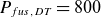
 $800$
MW deuterium–tritium fusion plasma with high fusion gain (
$800$
MW deuterium–tritium fusion plasma with high fusion gain ( $Q_{{fus}}\gtrsim 40$
), averaged density set by the Sudo limit (
$Q_{{fus}}\gtrsim 40$
), averaged density set by the Sudo limit ( $f_{{Sudo}} = \langle n_e\rangle /n_{{Sudo}} \sim 1$
), assuming an energy confinement time with some improvement over the ISS04 scaling law (
$f_{{Sudo}} = \langle n_e\rangle /n_{{Sudo}} \sim 1$
), assuming an energy confinement time with some improvement over the ISS04 scaling law ( $f_c \gt 1$
). The resulting configuration parameters are summarized in table 1. The major radius is
$f_c \gt 1$
). The resulting configuration parameters are summarized in table 1. The major radius is $R = 12.5$
m, the minor radius is
$R = 12.5$
m, the minor radius is $a = 1.25$
m and the average magnetic field on-axis is
$a = 1.25$
m and the average magnetic field on-axis is $B_{{axis}}=9$
T. This provides access to electron cyclotron resonance heating (ECRH) heating at 8.42 T (
$B_{{axis}}=9$
T. This provides access to electron cyclotron resonance heating (ECRH) heating at 8.42 T ( $B_{{axis,min}}/B_{{axis,max}}$
= 7.2 T/ 11.8 T) assuming availability of reliable, high-power 236 GHz gyrotrons (Thumm et al. Reference Thumm, Denisov, Sakamoto and Tran2019; Jelonnek et al. Reference Jelonnek2017). The rotational transform at the boundary is designed to be very close to the
$B_{{axis,min}}/B_{{axis,max}}$
= 7.2 T/ 11.8 T) assuming availability of reliable, high-power 236 GHz gyrotrons (Thumm et al. Reference Thumm, Denisov, Sakamoto and Tran2019; Jelonnek et al. Reference Jelonnek2017). The rotational transform at the boundary is designed to be very close to the $\iota _a = 0.8 = 4/5$
surface to enable an island divertor (Bader et al. Reference Bader2025), with very low global magnetic shear (
$\iota _a = 0.8 = 4/5$
surface to enable an island divertor (Bader et al. Reference Bader2025), with very low global magnetic shear ( $\iota _{min} \gt 0.75$
) to avoid the 3/4 rational surface.
$\iota _{min} \gt 0.75$
) to avoid the 3/4 rational surface.
Summary of Infinity Two configuration parameters.
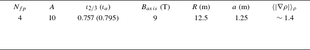
The free-boundary equilibrium self-consistently includes MHD and bootstrap currents using assumed profile shapes (Schmitt et al. Reference Schmitt2025). Unless noted otherwise, the equilibrium is held fixed for the analysis in this paper. The assumed profiles used to generate the equilibrium are shown in figure 1, with plasma parameters summarized in table 2. The volume-averaged electron density $\langle n_e \rangle = 1.8 \times 10^{20}$
m
$\langle n_e \rangle = 1.8 \times 10^{20}$
m $^{-3}$
corresponds to
$^{-3}$
corresponds to $f_{{Sudo}}=\langle n_e \rangle /n_{{Sudo}}=0.84$
and a boundary density
$f_{{Sudo}}=\langle n_e \rangle /n_{{Sudo}}=0.84$
and a boundary density $n_{{sep}} = 0.28\, n_{{Sudo}}$
. The boundary density is small relative to the Sudo density, providing headroom to increase it as needed to support a higher edge radiation fraction required for the plasma exhaust solution (Bader et al. Reference Bader2025) while sustaining elevated performance. The total beta
$n_{{sep}} = 0.28\, n_{{Sudo}}$
. The boundary density is small relative to the Sudo density, providing headroom to increase it as needed to support a higher edge radiation fraction required for the plasma exhaust solution (Bader et al. Reference Bader2025) while sustaining elevated performance. The total beta $\langle \beta \rangle = 1.63 \,\%$
is below the
$\langle \beta \rangle = 1.63 \,\%$
is below the $\langle \beta \rangle = 3.2\,\%$
global stability limit as found by Schmitt et al. (Reference Schmitt2025). We also estimate the ideal ballooning mode (IBM) stability threshold on the pressure gradient (
$\langle \beta \rangle = 3.2\,\%$
global stability limit as found by Schmitt et al. (Reference Schmitt2025). We also estimate the ideal ballooning mode (IBM) stability threshold on the pressure gradient ( $\beta '$
), shown in figure 1(f). The stability threshold is computed by first generating a series of global equilibria at increasing beta using the same assumed pressure profile shape (Schmitt et al. Reference Schmitt2025), and from this we find that the marginally stable equilibrium has
$\beta '$
), shown in figure 1(f). The stability threshold is computed by first generating a series of global equilibria at increasing beta using the same assumed pressure profile shape (Schmitt et al. Reference Schmitt2025), and from this we find that the marginally stable equilibrium has $\langle \beta \rangle = 2\,\%$
. The local stability limits are subsequently computed by local variation of the pressure gradient using the benchmarked Julia port of COBRAVMEC (Sanchez et al. (Reference Sanchez, Hirshman, Whitson and Ware2000), also described in Schmitt et al. (Reference Schmitt2025)). We note that profiles with less steep pressure gradients, such as the ones we predict in § 4, can lead to a higher stability limit, and thus the IBM threshold shown in figure 1(f) should be considered as a conservative estimate of IBM stability. The density profile is assumed to be flat inside
$\langle \beta \rangle = 2\,\%$
. The local stability limits are subsequently computed by local variation of the pressure gradient using the benchmarked Julia port of COBRAVMEC (Sanchez et al. (Reference Sanchez, Hirshman, Whitson and Ware2000), also described in Schmitt et al. (Reference Schmitt2025)). We note that profiles with less steep pressure gradients, such as the ones we predict in § 4, can lead to a higher stability limit, and thus the IBM threshold shown in figure 1(f) should be considered as a conservative estimate of IBM stability. The density profile is assumed to be flat inside $\rho \lt 0.6$
, with a transition to a region of steepening gradient moving radially outward, as is expected for pellet fuelling with penetration depth outside the midradius. With this profile shape the peaking factor is
$\rho \lt 0.6$
, with a transition to a region of steepening gradient moving radially outward, as is expected for pellet fuelling with penetration depth outside the midradius. With this profile shape the peaking factor is $n_0/\langle n \rangle =1.37$
and the ratio of axis to separatrix density is
$n_0/\langle n \rangle =1.37$
and the ratio of axis to separatrix density is $n_0/n_{{sep}}=4.0$
. The assumed electron temperature profile has a separatrix temperature
$n_0/n_{{sep}}=4.0$
. The assumed electron temperature profile has a separatrix temperature $T_{{sep}}=100\,\mathrm{eV}$
and has a peaking factor
$T_{{sep}}=100\,\mathrm{eV}$
and has a peaking factor $T_{e0}/\langle T_e \rangle =2.3$
, with
$T_{e0}/\langle T_e \rangle =2.3$
, with $T_{e0}/T_{i0} = 1.25$
on axis. Here,
$T_{e0}/T_{i0} = 1.25$
on axis. Here, $\langle A \rangle$
denotes the volume average of
$\langle A \rangle$
denotes the volume average of $A$
. The normalized gyroradius
$A$
. The normalized gyroradius $\rho _*$
and collisionality
$\rho _*$
and collisionality $\nu _*$
shown in table 2 are calculated for a deuterium ion according to the definitions in Alonso et al. (Reference Alonso, Calvo, Carralero, Velasco, García-Regaña, Palermo and Rapisarda2022) and using the volume averaged density and temperature and average magnetic field on axis.
$\nu _*$
shown in table 2 are calculated for a deuterium ion according to the definitions in Alonso et al. (Reference Alonso, Calvo, Carralero, Velasco, García-Regaña, Palermo and Rapisarda2022) and using the volume averaged density and temperature and average magnetic field on axis.
Summary of plasma parameters for the preliminary profiles shown in figure 1.
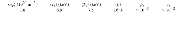
Preliminary assumed profiles used for configuration optimization, sizing and free-boundary equilibrium calculation.
3.2. Turbulence characteristics
Turbulent transport properties for the Infinity Two configuration are computed via nonlinear gyrokinetic calculations. Several parameter scans are performed using the GX codeFootnote
1
(Mandell et al. Reference Mandell, Dorland and Landreman2018, Reference Mandell, Dorland, Abel, Gaur, Kim, Martin and Qian2024), which solves the nonlinear gyrokinetic-Maxwell equations in the radially local (small $\rho _*$
) limit (Sugama & Horton Reference Sugama and Horton1998; Abel et al. Reference Abel, Plunk, Wang, Barnes, Cowley, Dorland and Schekochihin2013). Fourier pseudospectral decomposition is used in the three spatial dimensions
$\rho _*$
) limit (Sugama & Horton Reference Sugama and Horton1998; Abel et al. Reference Abel, Plunk, Wang, Barnes, Cowley, Dorland and Schekochihin2013). Fourier pseudospectral decomposition is used in the three spatial dimensions $(x,y,z)$
of the flux-tube domain, with
$(x,y,z)$
of the flux-tube domain, with $x$
the radial coordinate,
$x$
the radial coordinate, $y$
the binormal coordinate and
$y$
the binormal coordinate and $z=\theta$
the parallel coordinate, with
$z=\theta$
the parallel coordinate, with $\theta$
the straight-field-line poloidal angle. Pseudospectral decompositions are also used in velocity space, with a Hermite decomposition for parallel velocity (
$\theta$
the straight-field-line poloidal angle. Pseudospectral decompositions are also used in velocity space, with a Hermite decomposition for parallel velocity ( $He_m (v_{\parallel })$
) and a Laguerre decomposition for perpendicular energy (
$He_m (v_{\parallel })$
) and a Laguerre decomposition for perpendicular energy ( $L_\ell (\mu B)$
). Several numerical resolutions were tested to ensure that perpendicular spectra and parallel structure features are robustly captured, and that time-averaged quantitative transport changes less than 30 %. The base numerical resolution and domain lengths used for all GX cases in this work are summarized in table 4. Given the small values of global magnetic shear (|
$L_\ell (\mu B)$
). Several numerical resolutions were tested to ensure that perpendicular spectra and parallel structure features are robustly captured, and that time-averaged quantitative transport changes less than 30 %. The base numerical resolution and domain lengths used for all GX cases in this work are summarized in table 4. Given the small values of global magnetic shear (| $\hat {s}| \leqslant$
) 0.1 across much of the device radius, the generalized twist and shift boundary conditions (Martin et al. Reference Martin, Landreman, Xanthopoulos, Mandell and Dorland2018) have been used. The parallel domain along a chosen field line, labelled by
$\hat {s}| \leqslant$
) 0.1 across much of the device radius, the generalized twist and shift boundary conditions (Martin et al. Reference Martin, Landreman, Xanthopoulos, Mandell and Dorland2018) have been used. The parallel domain along a chosen field line, labelled by $\alpha = \theta - \iota \phi$
with
$\alpha = \theta - \iota \phi$
with $\iota$
the rational transform and
$\iota$
the rational transform and $\phi$
the toroidal angle, is chosen to extend a distance in
$\phi$
the toroidal angle, is chosen to extend a distance in $\theta$
corresponding to an equivalent of at least a 1.0 poloidal turn, with the precise length set to allow a perpendicular box with aspect ratio
$\theta$
corresponding to an equivalent of at least a 1.0 poloidal turn, with the precise length set to allow a perpendicular box with aspect ratio $L_x=L_y$
(Mandell et al. Reference Mandell, Dorland, Abel, Gaur, Kim, Martin and Qian2024). For the simulations in this paper the
$L_x=L_y$
(Mandell et al. Reference Mandell, Dorland, Abel, Gaur, Kim, Martin and Qian2024). For the simulations in this paper the $\alpha =0$
field line is chosen as tests show it produces transport
$\alpha =0$
field line is chosen as tests show it produces transport $\sim 30\,\%$
larger compared with the
$\sim 30\,\%$
larger compared with the $\alpha =\iota \pi /4$
field line.
$\alpha =\iota \pi /4$
field line.
The $\beta$
normalized collision frequencies and gradients for the radial positions used in the gyrokinetic analysis in this section.
$\beta$
normalized collision frequencies and gradients for the radial positions used in the gyrokinetic analysis in this section.
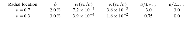

The simulations in this section use two kinetic species: electrons, and a single ion species with effective mass number $m_i/m_{{proton}} = 2.5$
to represent a 50:50 deuterium–tritium mix (Belli & Candy Reference Belli and Candy2021). We assume
$m_i/m_{{proton}} = 2.5$
to represent a 50:50 deuterium–tritium mix (Belli & Candy Reference Belli and Candy2021). We assume $n_i/n_e=1$
,
$n_i/n_e=1$
, $T_e/T_i=1$
,
$T_e/T_i=1$
, $a/L_{Te}=a/L_{Ti}$
,
$a/L_{Te}=a/L_{Ti}$
, $a/L_{n,i}=a/L_{n,e}$
. Full EM effects are modelled, including both shear
$a/L_{n,i}=a/L_{n,e}$
. Full EM effects are modelled, including both shear $\delta A_{\parallel }$
and compressional
$\delta A_{\parallel }$
and compressional $\delta B_{\parallel }$
magnetic perturbations, as well as intraspecies collisions (we neglect interspecies collisions) using the Dougherty collision operator (Dougherty Reference Dougherty1964). In other words, ion–ion and electron–electron collisions are simulated but not electron–ion. Values for
$\delta B_{\parallel }$
magnetic perturbations, as well as intraspecies collisions (we neglect interspecies collisions) using the Dougherty collision operator (Dougherty Reference Dougherty1964). In other words, ion–ion and electron–electron collisions are simulated but not electron–ion. Values for $\beta$
and
$\beta$
and $\nu _{s}$
, the intraspecies Coulomb collision frequency, are computed using the assumed profile shapes and are given in table 3. The Coulomb collision frequency is calculated using
$\nu _{s}$
, the intraspecies Coulomb collision frequency, are computed using the assumed profile shapes and are given in table 3. The Coulomb collision frequency is calculated using $\nu _s=(1/3\epsilon _0)\sqrt {1/8\pi ^3}Z_s^4e^4m_s^{-0.5}n_sT_s^{-3/2}\ln (\Lambda )$
, with
$\nu _s=(1/3\epsilon _0)\sqrt {1/8\pi ^3}Z_s^4e^4m_s^{-0.5}n_sT_s^{-3/2}\ln (\Lambda )$
, with $\epsilon _0$
the vacuum permittivity,
$\epsilon _0$
the vacuum permittivity, $Z_s$
the species charge number,
$Z_s$
the species charge number, $e$
the electron charge,
$e$
the electron charge, $m_s$
the species mass,
$m_s$
the species mass, $n_s$
its particle density,
$n_s$
its particle density, $T_s$
its temperature and
$T_s$
its temperature and $\ln (\Lambda )$
the Coulomb logarithm. The collision frequencies are then normalized by
$\ln (\Lambda )$
the Coulomb logarithm. The collision frequencies are then normalized by $a/v_{ti}$
where
$a/v_{ti}$
where $a$
is the configuration minor radius and
$a$
is the configuration minor radius and $v_{ti}$
is the local ion thermal velocity.
$v_{ti}$
is the local ion thermal velocity.
We report normalized radial heat fluxes defined as
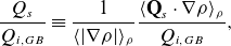 \begin{equation} \frac {{Q}_s}{Q_{i,GB}} \equiv \frac {1}{\langle |\nabla \rho |\rangle _\rho }\frac {\langle \textbf {Q}_s\cdot \nabla \rho \rangle _\rho }{Q_{i,GB}}, \end{equation}
where $\textbf {Q}_s\cdot \nabla \rho$
is the turbulence time-averaged radial heat flux moment of the gyrokinetic distribution function,
$\textbf {Q}_s\cdot \nabla \rho$
is the turbulence time-averaged radial heat flux moment of the gyrokinetic distribution function, $Q_{i,\mathrm {GB}}= n_i T_i v_{ti}\rho _i^2/a^2$
is the local gyroBohm heat flux for deuterium–tritium ions,
$Q_{i,\mathrm {GB}}= n_i T_i v_{ti}\rho _i^2/a^2$
is the local gyroBohm heat flux for deuterium–tritium ions, $\langle \cdot \rangle _\rho$
denotes a flux-surface average and the factor
$\langle \cdot \rangle _\rho$
denotes a flux-surface average and the factor $\langle |\nabla \rho | \rangle _\rho$
is included so that the choice of radial coordinate
$\langle |\nabla \rho | \rangle _\rho$
is included so that the choice of radial coordinate $\rho$
does not affect how the normalized heat flux enters the energy transport equation; for additional details, see the discussion around (4.2) and (4.3). The factor
$\rho$
does not affect how the normalized heat flux enters the energy transport equation; for additional details, see the discussion around (4.2) and (4.3). The factor $\langle |\nabla \rho | \rangle _\rho \sim 1.4$
across most of the cross-section is greater than unity owing to elongation and shaping effects. Note that we adopt the GX convention for the definition of the thermal velocity,
$\langle |\nabla \rho | \rangle _\rho \sim 1.4$
across most of the cross-section is greater than unity owing to elongation and shaping effects. Note that we adopt the GX convention for the definition of the thermal velocity, $v_{ts} = \sqrt {T_s/m_s}$
(without a factor of 2); since
$v_{ts} = \sqrt {T_s/m_s}$
(without a factor of 2); since $Q_{i,\mathrm {GB}}\sim v_{ti}\rho _i^2 \sim v_{ti}^3$
, a factor of
$Q_{i,\mathrm {GB}}\sim v_{ti}\rho _i^2 \sim v_{ti}^3$
, a factor of $\sqrt {2}$
difference in
$\sqrt {2}$
difference in $v_t$
results in a factor of
$v_t$
results in a factor of $\sqrt {8}$
difference in heat fluxes, which must be accounted for when comparing gyroBohm-normalized fluxes with different
$\sqrt {8}$
difference in heat fluxes, which must be accounted for when comparing gyroBohm-normalized fluxes with different $v_t$
definitions.
$v_t$
definitions.
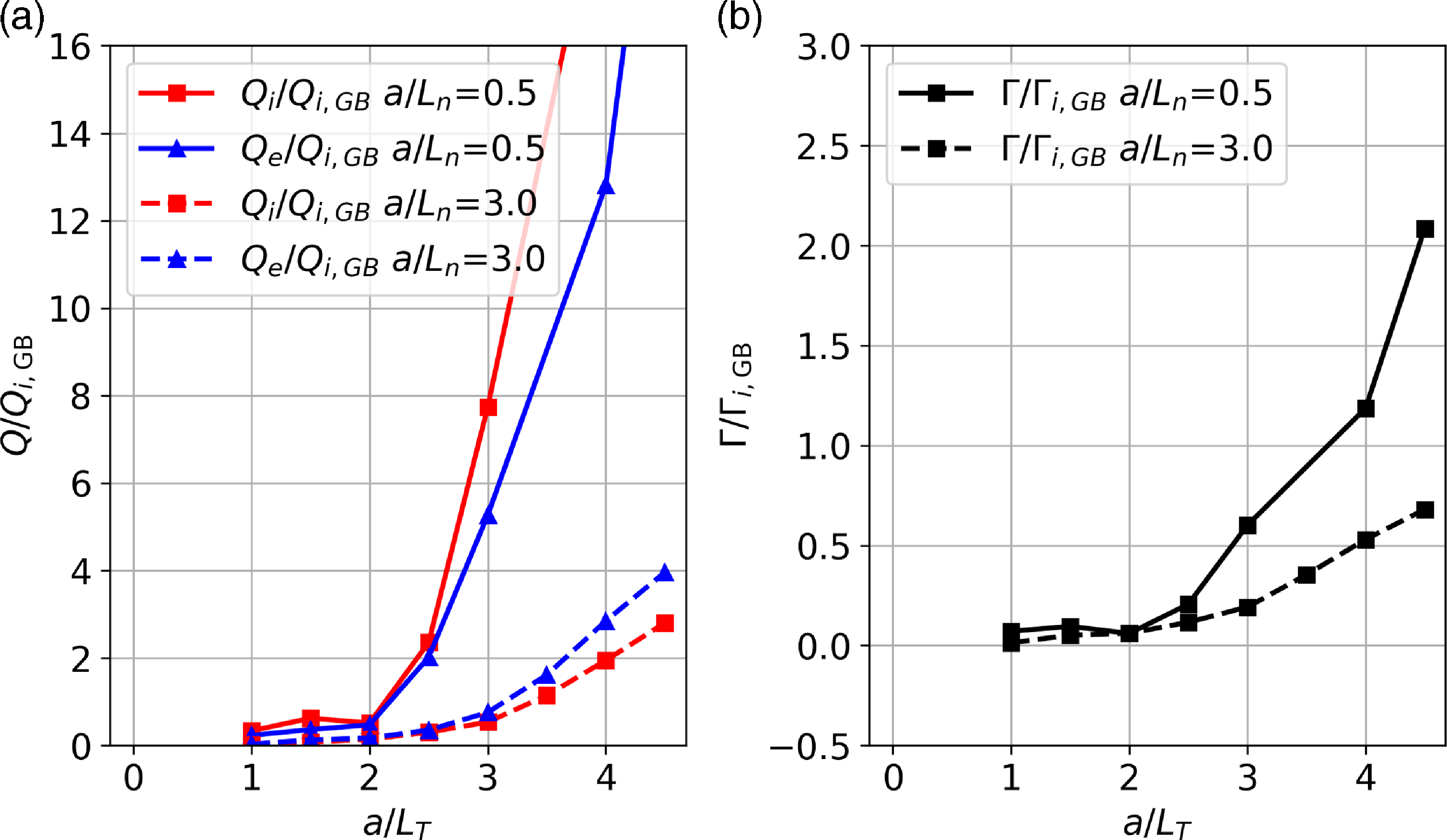
(a) Electron (blue) and ion (red) heat flux and (b) particle flux versus normalized temperature gradient ( $a/L_{Te}=a/L_{Ti}$
) for parameters representative of
$a/L_{Te}=a/L_{Ti}$
) for parameters representative of $\rho$
=0.7 at two values of density gradient (
$\rho$
=0.7 at two values of density gradient ( $a/L_n=0.5$
in solid line and
$a/L_n=0.5$
in solid line and $a/L_n=3$
in dashed line).
$a/L_n=3$
in dashed line).
Simulations are run at $\rho =0.7$
(
$\rho =0.7$
( $\beta$
= 2.0 %), in the region of assumed large density gradient, as this radius is representative of global energy confinement characteristics as discussed above. Additional simulations are run at
$\beta$
= 2.0 %), in the region of assumed large density gradient, as this radius is representative of global energy confinement characteristics as discussed above. Additional simulations are run at $\rho =0.3$
(
$\rho =0.3$
( $\beta$
= 3.0 %) to illustrate transport properties deeper in the core where the density gradient is expected to be very close to flat in the assumed operating scenario. When performing gradient scans, equilibrium quantities are varied self-consistently local to a magnetic flux surface as
$\beta$
= 3.0 %) to illustrate transport properties deeper in the core where the density gradient is expected to be very close to flat in the assumed operating scenario. When performing gradient scans, equilibrium quantities are varied self-consistently local to a magnetic flux surface as $\beta '$
is varied, following the approach of Hegna & Nakajima (Reference Hegna and Nakajima1998). This approach does not recompute a self-consistent global equilibrium, and thus does not include variations in global effects like Shafranov shift.
$\beta '$
is varied, following the approach of Hegna & Nakajima (Reference Hegna and Nakajima1998). This approach does not recompute a self-consistent global equilibrium, and thus does not include variations in global effects like Shafranov shift.
Temperature gradient scans evaluated at $\rho =0.7$
are shown in figure 2. With a weak density gradient (
$\rho =0.7$
are shown in figure 2. With a weak density gradient ( $a/L_n$
= 0.5), the simulations show there is a range of relatively small transport above the linear threshold
$a/L_n$
= 0.5), the simulations show there is a range of relatively small transport above the linear threshold $a/L_T \lt 1$
. However, above
$a/L_T \lt 1$
. However, above $a/L_T \gt 2$
the transport increases very rapidly, more characteristic of undesirably stiff ITG transport. An additional scan is run at larger
$a/L_T \gt 2$
the transport increases very rapidly, more characteristic of undesirably stiff ITG transport. An additional scan is run at larger $a/L_n=3$
, similar to the values achieved around the same radius in W7-X pellet-fuelled discharges (Baldzuhn et al. Reference Baldzuhn2020; Carralero et al. Reference Carralero2021). Although linearly unstable modes still exist at small
$a/L_n=3$
, similar to the values achieved around the same radius in W7-X pellet-fuelled discharges (Baldzuhn et al. Reference Baldzuhn2020; Carralero et al. Reference Carralero2021). Although linearly unstable modes still exist at small $a/L_T$
, the transport saturates at much lower magnitude and exhibits much lower stiffness. As a result, up to
$a/L_T$
, the transport saturates at much lower magnitude and exhibits much lower stiffness. As a result, up to $\approx$
50 % larger temperature gradients should be achievable for power plant transport levels expected near this radius,
$\approx$
50 % larger temperature gradients should be achievable for power plant transport levels expected near this radius, $Q/Q_{GB} \approx$
1–2. It is these conditions that lead to improved confinement and are targeted via configuration optimization assuming an increased density gradient. Using the simple criteria discussed in § 2.1, the resulting
$Q/Q_{GB} \approx$
1–2. It is these conditions that lead to improved confinement and are targeted via configuration optimization assuming an increased density gradient. Using the simple criteria discussed in § 2.1, the resulting $Q_{tot,(a/L_T=3)}/Q_{GB} \approx 1.5$
suggests
$Q_{tot,(a/L_T=3)}/Q_{GB} \approx 1.5$
suggests $f_c \geqslant 1$
may be possible in this configuration and operating scenario, which is confirmed from the profile predictions in § 4.
$f_c \geqslant 1$
may be possible in this configuration and operating scenario, which is confirmed from the profile predictions in § 4.
(a) Electron (blue) and ion (red) heat flux, (b) particle flux and (c) ratio between the particle flux and the total heat flux versus normalized density gradient ( $a/L_n$
) for parameters representative of
$a/L_n$
) for parameters representative of $\rho$
=0.7. The solid curve was obtained using the nominal
$\rho$
=0.7. The solid curve was obtained using the nominal $\beta$
and EM effects while the dashed curve was obtained in the electrostatic limit with
$\beta$
and EM effects while the dashed curve was obtained in the electrostatic limit with $\beta =0.1\,\%$
while suppressing the compressional
$\beta =0.1\,\%$
while suppressing the compressional $\delta B_{\parallel }$
magnetic perturbations.
$\delta B_{\parallel }$
magnetic perturbations.
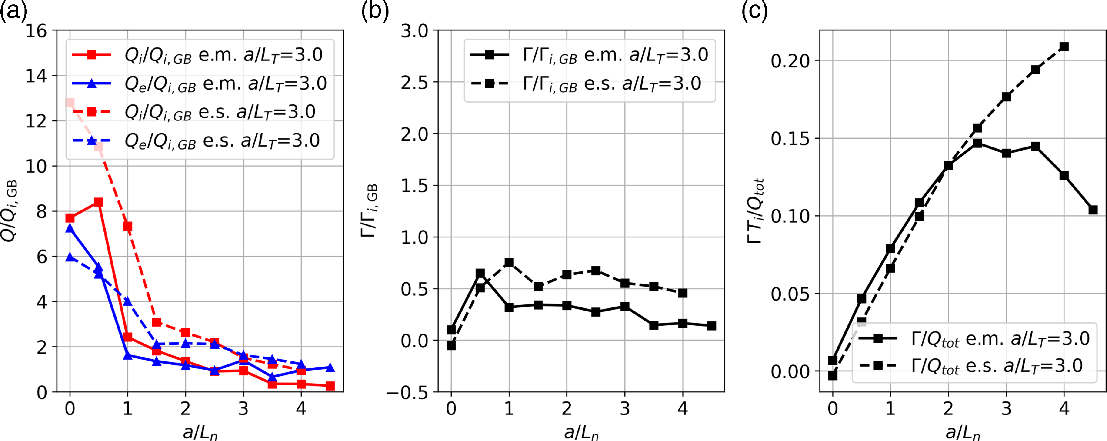
To directly illustrate the impact of density gradient on the resulting transport, a scan of $a/L_n$
is performed for fixed
$a/L_n$
is performed for fixed $a/L_T=3$
. Figure 3 shows the stabilization begins to occur at small values of
$a/L_T=3$
. Figure 3 shows the stabilization begins to occur at small values of $a/L_n$
and becomes very strong for
$a/L_n$
and becomes very strong for $a/L_n \geqslant 1.5$
, or
$a/L_n \geqslant 1.5$
, or $\eta _i \leqslant 2.0$
. Stabilization continues up to at least
$\eta _i \leqslant 2.0$
. Stabilization continues up to at least $a/L_n$
= 4 (
$a/L_n$
= 4 ( $\eta _i = 0.75$
). Similar nonlinear results have been reported more recently for W7-X, NCSX (Thienpondt et al. Reference Thienpondt, García-Regaña, Calvo, Acton and Barnes2024b
) and CIEMAT-QI4 (García-Regaña et al. Reference García-Regaña, Calvo, Parra and Thienpondt2024). Up to the range of values simulated, the ion thermal transport decreases continuously, consistent with the expected suppression of ITG turbulence. The electron thermal transport also decreases substantially but appears to level off to a nearly constant value, eventually overtaking the ion transport,
$\eta _i = 0.75$
). Similar nonlinear results have been reported more recently for W7-X, NCSX (Thienpondt et al. Reference Thienpondt, García-Regaña, Calvo, Acton and Barnes2024b
) and CIEMAT-QI4 (García-Regaña et al. Reference García-Regaña, Calvo, Parra and Thienpondt2024). Up to the range of values simulated, the ion thermal transport decreases continuously, consistent with the expected suppression of ITG turbulence. The electron thermal transport also decreases substantially but appears to level off to a nearly constant value, eventually overtaking the ion transport, $Q_e/Q_i \gt 1$
. The relative strength of particle flux,
$Q_e/Q_i \gt 1$
. The relative strength of particle flux, $\Gamma T/Q_{tot}$
, also increases with increasing density gradient. These changes in transport characteristics suggest there is increasing contribution from non-adiabatic trapped electron dynamics. The potential minimum transport between ITG and TEM dominant regimes is reminiscent of the so-called ‘stability valley’ predicted around a similar range of
$\Gamma T/Q_{tot}$
, also increases with increasing density gradient. These changes in transport characteristics suggest there is increasing contribution from non-adiabatic trapped electron dynamics. The potential minimum transport between ITG and TEM dominant regimes is reminiscent of the so-called ‘stability valley’ predicted around a similar range of $\eta _i$
in W7-X (Alcusón et al. Reference Alcusón, Xanthopoulos, Plunk, Helander, Wilms, Turkin, Stechow and Grulke2020; Xanthopoulos et al. Reference Xanthopoulos2020).
$\eta _i$
in W7-X (Alcusón et al. Reference Alcusón, Xanthopoulos, Plunk, Helander, Wilms, Turkin, Stechow and Grulke2020; Xanthopoulos et al. Reference Xanthopoulos2020).
To further characterize the turbulence, in figure 4 we compare the parallel structure of the time-averaged heat flux with the parallel structure in the magnitude of the magnetic field ( $B/B_{ref}$
, with
$B/B_{ref}$
, with $B_{{ref}}=2\psi _{{LCFS}}/a^2$
) and normal curvature, parametrized by the binormal curvature drift coefficient
$B_{{ref}}=2\psi _{{LCFS}}/a^2$
) and normal curvature, parametrized by the binormal curvature drift coefficient $\kappa _\alpha =((\mathbf {b}\times \nabla B)\cdot \nabla \alpha +8\pi (\mathbf {b}\times \nabla \alpha )\cdot \nabla p)/B^2$
. We make this comparison for a case with weak density gradient and another case with strong density gradient, with the temperature gradients chosen in each case so that the two cases have similar magnitude of heat flux. In the weak density gradient case (
$\kappa _\alpha =((\mathbf {b}\times \nabla B)\cdot \nabla \alpha +8\pi (\mathbf {b}\times \nabla \alpha )\cdot \nabla p)/B^2$
. We make this comparison for a case with weak density gradient and another case with strong density gradient, with the temperature gradients chosen in each case so that the two cases have similar magnitude of heat flux. In the weak density gradient case ( $a/L_n=0.5$
, solid lines),
$a/L_n=0.5$
, solid lines), $Q(\theta )$
has two local maxima on either side of
$Q(\theta )$
has two local maxima on either side of $\theta =0$
, aligned with the peaks in maximum bad curvature (red curves in figure 4
b) where ITG drive is strongest. For the strong density gradient case (
$\theta =0$
, aligned with the peaks in maximum bad curvature (red curves in figure 4
b) where ITG drive is strongest. For the strong density gradient case ( $a/L_n=3$
, dotted lines), the peaks in
$a/L_n=3$
, dotted lines), the peaks in $Q(\theta )$
are shifted slightly farther away from
$Q(\theta )$
are shifted slightly farther away from $\theta =0$
, and are more closely aligned with the local minima in |B| where contributions from trapped electron resonances are expected to be strongest. The shift in parallel structure is consistent with strong ITG dynamics being stabilized with increasing density gradient, which leads to dynamics typically associated with a TEM-like response. The increase in
$\theta =0$
, and are more closely aligned with the local minima in |B| where contributions from trapped electron resonances are expected to be strongest. The shift in parallel structure is consistent with strong ITG dynamics being stabilized with increasing density gradient, which leads to dynamics typically associated with a TEM-like response. The increase in $\beta '$
is also seen to favourably impact the normalized curvature in many regions (as computed from the local equilibrium expansion of Hegna & Nakajima (Reference Hegna and Nakajima1998)), likely contributing additional stabilization as noted in García-Regaña et al. (Reference García-Regaña, Calvo, Parra and Thienpondt2024); e.g. the magnitude of bad curvature is reduced around
$\beta '$
is also seen to favourably impact the normalized curvature in many regions (as computed from the local equilibrium expansion of Hegna & Nakajima (Reference Hegna and Nakajima1998)), likely contributing additional stabilization as noted in García-Regaña et al. (Reference García-Regaña, Calvo, Parra and Thienpondt2024); e.g. the magnitude of bad curvature is reduced around $|\theta | \approx 0.5\pi$
, and the good curvature around
$|\theta | \approx 0.5\pi$
, and the good curvature around $|\theta | \sim 0.3\pi$
is further deepened.
$|\theta | \sim 0.3\pi$
is further deepened.
(a) Electron (blue) and ion (red) heat-fluxes along the flux-tube for two sets of density and temperature gradients ( $a/L_n=0.5$
,
$a/L_n=0.5$
, $a/{L_T}=2.5$
in solid and
$a/{L_T}=2.5$
in solid and $a/L_n=3.0$
,
$a/L_n=3.0$
, $a/{L_T}=4.0$
in dashed). (b) Relative magnetic field amplitude
$a/{L_T}=4.0$
in dashed). (b) Relative magnetic field amplitude $B/B_{{ref}}$
and normalized curvature drift coefficient,
$B/B_{{ref}}$
and normalized curvature drift coefficient, $\kappa _\alpha =((\mathbf {b}\times \nabla B)\cdot \nabla \alpha +8\pi (\mathbf {b}\times \nabla \alpha )\cdot \nabla p)/B^2$
, as a function of the poloidal angle
$\kappa _\alpha =((\mathbf {b}\times \nabla B)\cdot \nabla \alpha +8\pi (\mathbf {b}\times \nabla \alpha )\cdot \nabla p)/B^2$
, as a function of the poloidal angle $\theta$
along the magnetic field line at
$\theta$
along the magnetic field line at $\rho =0.7$
and
$\rho =0.7$
and $\alpha =0$
. Here
$\alpha =0$
. Here $B_{{ref}}=2\psi _{{edge}}/a^2$
. The variations in the geometric quantities between the two cases are due to the Hegna–Nakajima perturbation of the local equilibrium with the different gradients (Hegna & Nakajima Reference Hegna and Nakajima1998).
$B_{{ref}}=2\psi _{{edge}}/a^2$
. The variations in the geometric quantities between the two cases are due to the Hegna–Nakajima perturbation of the local equilibrium with the different gradients (Hegna & Nakajima Reference Hegna and Nakajima1998).
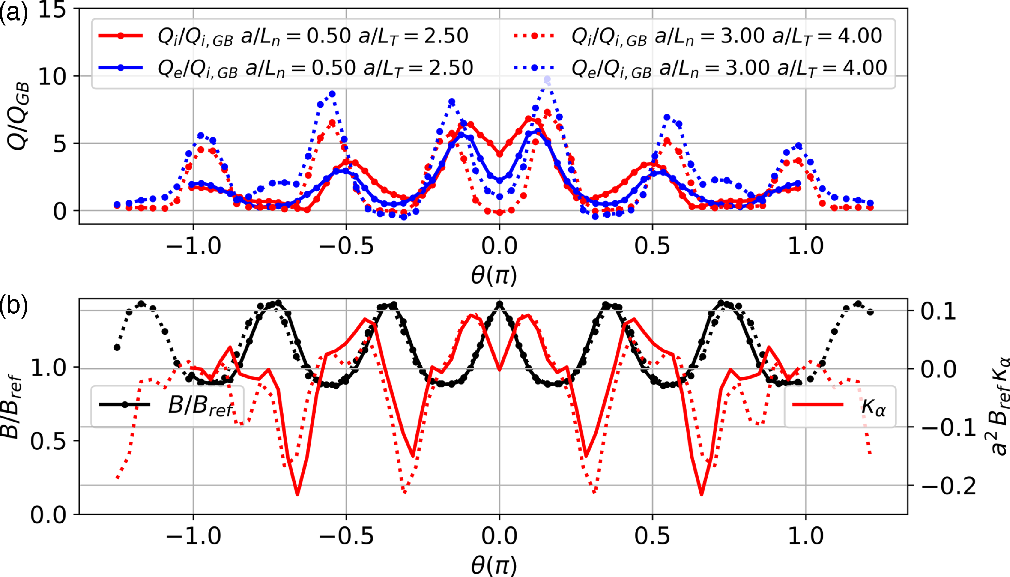
The ability to go to increasingly higher $a/L_n$
without sign of increasing thermal transport is consistent with having optimized for maximum-J properties (Hegna et al. Reference Hegna2025), which is expected to minimize trapped electron contributions that might otherwise cause instability (e.g. García-Regaña et al. Reference García-Regaña, Calvo, Parra and Thienpondt2024). However, the EM simulations here do predict that the magnetic flutter contributions become non-negligible, surpassing 25 % of the total electron thermal transport at the largest density gradients considered. The importance of EM effects is well known to strengthen as
$a/L_n$
without sign of increasing thermal transport is consistent with having optimized for maximum-J properties (Hegna et al. Reference Hegna2025), which is expected to minimize trapped electron contributions that might otherwise cause instability (e.g. García-Regaña et al. Reference García-Regaña, Calvo, Parra and Thienpondt2024). However, the EM simulations here do predict that the magnetic flutter contributions become non-negligible, surpassing 25 % of the total electron thermal transport at the largest density gradients considered. The importance of EM effects is well known to strengthen as $\beta '$
becomes a significant fraction of the ideal or KBM threshold (Snyder Reference Snyder1999; Aleynikova et al. Reference Aleynikova, Zocco, Xanthopoulos, Helander and Nührenberg2018; Mulholland et al. Reference Mulholland, Aleynikova, Faber, Pueschel, Proll, Hegna, Terry and Nührenberg2023), which is the case here. As seen in figure 1(f), the assumed profiles are predicted to be within
$\beta '$
becomes a significant fraction of the ideal or KBM threshold (Snyder Reference Snyder1999; Aleynikova et al. Reference Aleynikova, Zocco, Xanthopoulos, Helander and Nührenberg2018; Mulholland et al. Reference Mulholland, Aleynikova, Faber, Pueschel, Proll, Hegna, Terry and Nührenberg2023), which is the case here. As seen in figure 1(f), the assumed profiles are predicted to be within $\sim 30\,\%$
of the ideal MHD ballooning mode (IBM) limits. To quantify the impact of EM effects on the gyrokinetic simulations, an additional density gradient scan is performed with reduced
$\sim 30\,\%$
of the ideal MHD ballooning mode (IBM) limits. To quantify the impact of EM effects on the gyrokinetic simulations, an additional density gradient scan is performed with reduced $\beta$
= 0.1 % compared with the nominal
$\beta$
= 0.1 % compared with the nominal $\beta$
= 2 %. The compressional magnetic perturbations are also excluded,
$\beta$
= 2 %. The compressional magnetic perturbations are also excluded, $\delta B_{\parallel }$
= 0. The total thermal transport in these pseudoelectrostatic simulations is
$\delta B_{\parallel }$
= 0. The total thermal transport in these pseudoelectrostatic simulations is $1.5-2 \times$
larger than the EM simulations indicating a substantial stabilizing effect over the entire range of density gradients, figure 3.
$1.5-2 \times$
larger than the EM simulations indicating a substantial stabilizing effect over the entire range of density gradients, figure 3.
(a) Electron (blue) and ion (red) heat flux versus the local $\beta$
for parameters representative of
$\beta$
for parameters representative of $\rho$
=0.7 at
$\rho$
=0.7 at $a/L_n=3.0$
and
$a/L_n=3.0$
and $a/L_T=3.0$
. The heat fluxes are separated by field contribution: solid is total; dashed is
$a/L_T=3.0$
. The heat fluxes are separated by field contribution: solid is total; dashed is $\phi$
and dotted is
$\phi$
and dotted is $A_\parallel$
. The
$A_\parallel$
. The $B_\parallel$
contribution is not shown as it is negligible, and only the total
$B_\parallel$
contribution is not shown as it is negligible, and only the total $Q_i$
is shown as it is dominated by the
$Q_i$
is shown as it is dominated by the $\phi$
contribution. (b) The
$\phi$
contribution. (b) The $Q(k_y)$
spectra for three values of
$Q(k_y)$
spectra for three values of $\beta$
denoted by the line colour. Here, the total
$\beta$
denoted by the line colour. Here, the total $Q_i$
is shown with a solid line, the total
$Q_i$
is shown with a solid line, the total $Q_e$
with a dashed–dotted line, the electrostatic contribution
$Q_e$
with a dashed–dotted line, the electrostatic contribution $Q_{e,\phi }$
with a dashed line and the EM contribution
$Q_{e,\phi }$
with a dashed line and the EM contribution $Q_{e,A_\parallel }$
with a dotted line.
$Q_{e,A_\parallel }$
with a dotted line.
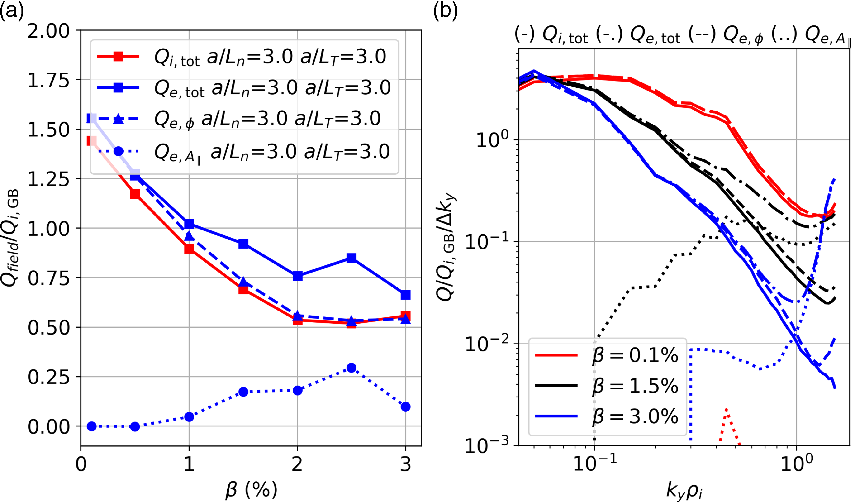
An additional scan varying only $\beta$
for fixed gradients (
$\beta$
for fixed gradients ( $a/L_T=3$
,
$a/L_T=3$
, $a/L_n=3$
) illustrates the EM stabilization occurs gradually from
$a/L_n=3$
) illustrates the EM stabilization occurs gradually from $\beta = 0\,\%-3 \,\%$
(figure 5
a). The electrostatic (
$\beta = 0\,\%-3 \,\%$
(figure 5
a). The electrostatic ( $Q_\phi$
) components of the electron and ion heat fluxes decrease by a factor of three over this range. A similar reduction of transport has been seen in W7-X EM simulations with increasing beta (Weir et al. Reference Weir2023). The growing contribution of electron flutter transport is found to occur at wavenumbers larger than
$Q_\phi$
) components of the electron and ion heat fluxes decrease by a factor of three over this range. A similar reduction of transport has been seen in W7-X EM simulations with increasing beta (Weir et al. Reference Weir2023). The growing contribution of electron flutter transport is found to occur at wavenumbers larger than $k_y\rho _i \gt 0.6-1$
, depending on beta (figure 5
b). A linear scan at the initially assumed
$k_y\rho _i \gt 0.6-1$
, depending on beta (figure 5
b). A linear scan at the initially assumed $\beta =2\,\%$
predicts the existence of unstable modes in this wavenumber range that propagate in the electron drift direction and exhibit highly elongated tearing-parity structure. Further work is required to understand the nature of these instabilities and whether they are responsible for the increasing flutter contribution in this regime. For even larger values of
$\beta =2\,\%$
predicts the existence of unstable modes in this wavenumber range that propagate in the electron drift direction and exhibit highly elongated tearing-parity structure. Further work is required to understand the nature of these instabilities and whether they are responsible for the increasing flutter contribution in this regime. For even larger values of $\beta \geqslant 3.5 \,\%$
, nonlinear simulations grow exponentially in time to very large transport (
$\beta \geqslant 3.5 \,\%$
, nonlinear simulations grow exponentially in time to very large transport ( $Q/Q_{GB}\gt 10^4$
) without showing signs of saturation. Linear simulations predict the onset of unstable KBM at the same values of
$Q/Q_{GB}\gt 10^4$
) without showing signs of saturation. Linear simulations predict the onset of unstable KBM at the same values of $\beta$
with features similar to those presented in recent studies (McKinney et al. Reference McKinney, Pueschel, Faber, Hegna, Ishizawa and Terry2021; Aleynikova et al. Reference Aleynikova, Zocco, Xanthopoulos, Helander and Nührenberg2018). The similarity between linear KBM, nonlinear KBM and IBM thresholds suggests there should be sufficient margin to avoid the onset of KBM in these regions of large local pressure gradient. In contrast, a more recent study (Mulholland et al. Reference Mulholland, Aleynikova, Faber, Pueschel, Proll, Hegna, Terry and Nührenberg2023, Reference Mulholland, Pueschel, Proll, Aleynikova, Faber, Terry, Hegna and Nührenberg2024) in W7-X finds there are conditions where a steady increase in transport with
$\beta$
with features similar to those presented in recent studies (McKinney et al. Reference McKinney, Pueschel, Faber, Hegna, Ishizawa and Terry2021; Aleynikova et al. Reference Aleynikova, Zocco, Xanthopoulos, Helander and Nührenberg2018). The similarity between linear KBM, nonlinear KBM and IBM thresholds suggests there should be sufficient margin to avoid the onset of KBM in these regions of large local pressure gradient. In contrast, a more recent study (Mulholland et al. Reference Mulholland, Aleynikova, Faber, Pueschel, Proll, Hegna, Terry and Nührenberg2023, Reference Mulholland, Pueschel, Proll, Aleynikova, Faber, Terry, Hegna and Nührenberg2024) in W7-X finds there are conditions where a steady increase in transport with $\beta$
is observed well below the linear onset of the dominant linear KBM instability. In that study, the increase in transport is correlated with the presence of a subdominant, subthreshold KBM. Additional future detailed analysis is required to more accurately compare exact thresholds, as well as the impact of self-consistently varying global equilibrium and thermal profile shapes, which was not addressed here.
$\beta$
is observed well below the linear onset of the dominant linear KBM instability. In that study, the increase in transport is correlated with the presence of a subdominant, subthreshold KBM. Additional future detailed analysis is required to more accurately compare exact thresholds, as well as the impact of self-consistently varying global equilibrium and thermal profile shapes, which was not addressed here.
Deeper in the core, $\rho \lt 0.5$
where there is no particle source (only a small sink from deuterium–tritium fusion) the electron and fuel ion density profiles are expected to be close to flat, depending on the details of any residual neoclassical thermodiffusion and ITG pinch. Furthermore, from simple power balance estimates in power plant conditions, the corresponding gyroBohm normalized heat fluxes are expected to be very small,
$\rho \lt 0.5$
where there is no particle source (only a small sink from deuterium–tritium fusion) the electron and fuel ion density profiles are expected to be close to flat, depending on the details of any residual neoclassical thermodiffusion and ITG pinch. Furthermore, from simple power balance estimates in power plant conditions, the corresponding gyroBohm normalized heat fluxes are expected to be very small, $Q/Q_{GB}\lt 1$
(see § 4). The resulting profiles will depend on matching zero or very small particle fluxes. To investigate this, additional scans are done at
$Q/Q_{GB}\lt 1$
(see § 4). The resulting profiles will depend on matching zero or very small particle fluxes. To investigate this, additional scans are done at $\rho = 0.3$
targeting these conditions.
$\rho = 0.3$
targeting these conditions.
(a) Electron (blue) and ion (red) heat flux and (b) particle flux versus normalized temperature gradient ( $a/L_{Te}=a/L_{Ti}$
) for parameters representative of
$a/L_{Te}=a/L_{Ti}$
) for parameters representative of $\rho$
=0.3 for
$\rho$
=0.3 for $a/L_n=0$
. The error bars show the standard deviation of the quantities around the time-averaged value.
$a/L_n=0$
. The error bars show the standard deviation of the quantities around the time-averaged value.
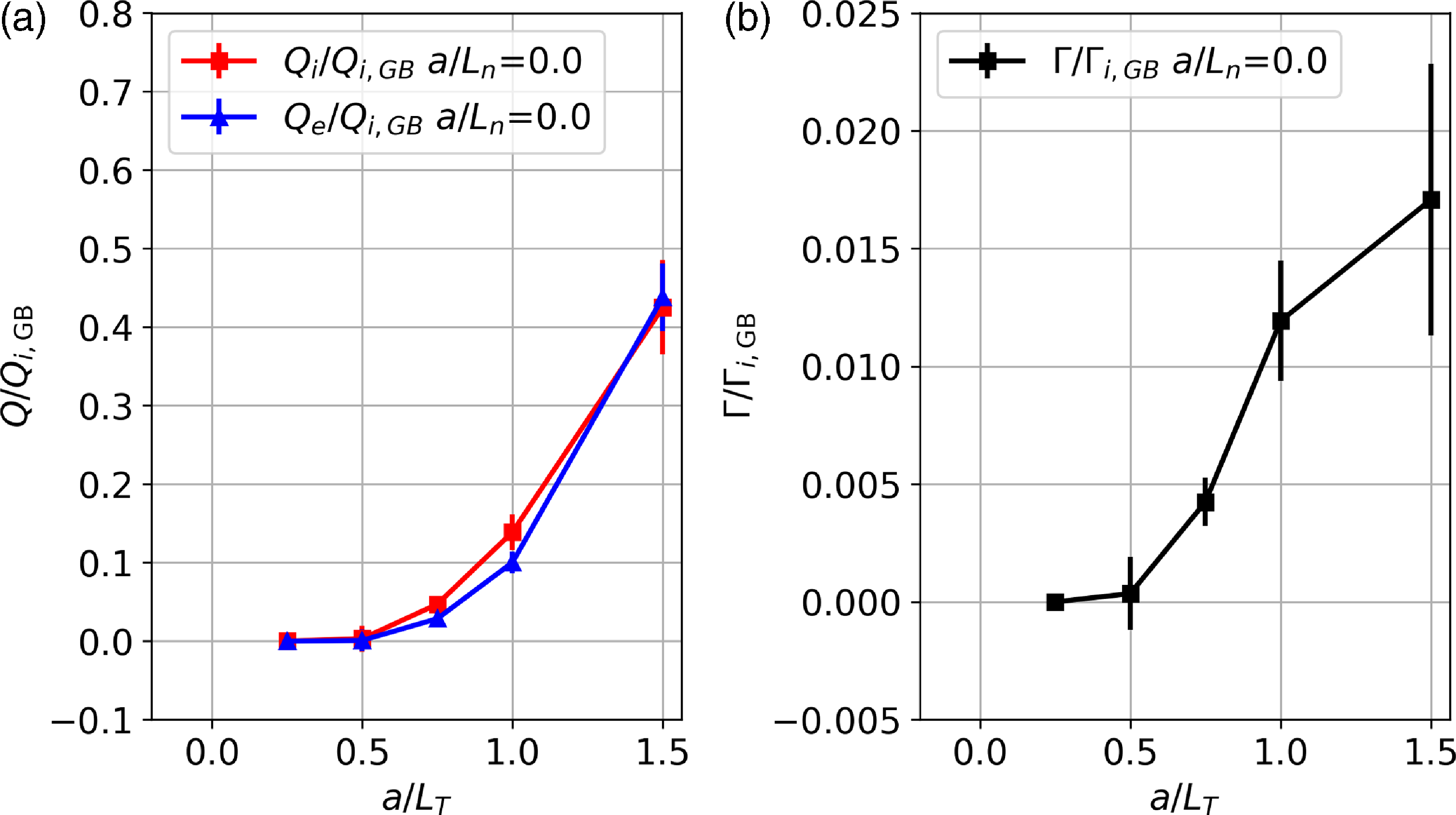
(a) Electron (blue) and ion (red) heat flux and (b) particle flux versus normalized density gradient ( $a/L_n$
) for parameters representative of
$a/L_n$
) for parameters representative of $\rho$
=0.3 with
$\rho$
=0.3 with $a/L_{Te}=a/L_{Ti}=0.75$
. The error bars show the standard deviation of the quantities around the time-averaged value.
$a/L_{Te}=a/L_{Ti}=0.75$
. The error bars show the standard deviation of the quantities around the time-averaged value.
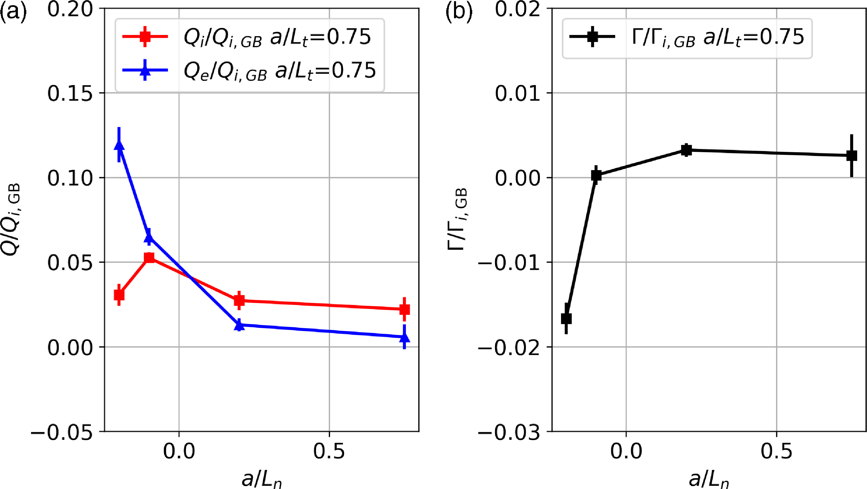
Figure 6 shows the predicted fluxes versus $a/L_T$
assuming no density gradient (
$a/L_T$
assuming no density gradient ( $a/L_n$
= 0), where an effective critical gradient around
$a/L_n$
= 0), where an effective critical gradient around $a/L_{T,crit} \approx$
0.5 is observed. Heat flux values remain below
$a/L_{T,crit} \approx$
0.5 is observed. Heat flux values remain below $Q/Q_{GB} \sim$
1 up to
$Q/Q_{GB} \sim$
1 up to $a/L_T = 1.5$
, so that profiles should remain relatively close to marginal. The corresponding particle flux is very small but outward in this regime, suggesting the ITG turbulence could in fact hollow the density instead of peaking it from an inward pinch as predicted in the core for W7-X analysis (Thienpondt et al. Reference Thienpondt2023). To assess the potential strength of this convection, a scan in density gradient was performed at fixed
$a/L_T = 1.5$
, so that profiles should remain relatively close to marginal. The corresponding particle flux is very small but outward in this regime, suggesting the ITG turbulence could in fact hollow the density instead of peaking it from an inward pinch as predicted in the core for W7-X analysis (Thienpondt et al. Reference Thienpondt2023). To assess the potential strength of this convection, a scan in density gradient was performed at fixed $a/L_T$
= 0.75, just above marginal. As shown in figure 7, very little density hollowing, −0.2 <
$a/L_T$
= 0.75, just above marginal. As shown in figure 7, very little density hollowing, −0.2 < $a/L_n$
<0, would be needed to satisfy the zero flux condition
$a/L_n$
<0, would be needed to satisfy the zero flux condition $\Gamma$
= 0. However, the dependence is complicated by the fact that reducing the density gradient tends to increase the overall thermal transport. Ultimately, self-consistent profile predictions are required to directly predict the expected density peaking or hollowing.
$\Gamma$
= 0. However, the dependence is complicated by the fact that reducing the density gradient tends to increase the overall thermal transport. Ultimately, self-consistent profile predictions are required to directly predict the expected density peaking or hollowing.
4. Profile predictions
The analysis in the previous section illustrates the reduced level of transport predicted for this optimized configuration assuming an operating regime with increased density gradient. Transport-based profile predictions are required to quantitatively predict energy confinement and fusion performance, which are described in this section. For the present work, we use a fixed density profile assumed to have edge peaking due to pellet fuelling. Additional analysis is presented to assess whether these density profiles are achievable based on pellet ablation calculations. Impurity transport characteristics are also predicted and discussed.
4.1. Transport modelling methods
We use the T3D transport solver to make high-fidelity profile predictions (Qian et al. Reference Qian, Buck, Gaur, Mandell, Kim and Dorland2022). The T3D solver uses a multiscale algorithm (Barnes et al. Reference Barnes, Abel, Dorland, Görler, Hammett and Jenko2010) to self-consistently evolve the equilibrium profiles (density and temperature) subject to first-principles turbulent and neoclassical transport. For the present work, we assume a fixed density profile with edge peaking and only evolve the electron and fuel ion temperature profiles. Self-consistent density profile prediction will be a key area of future work. In lieu of this, we provide additional analysis comparing pellet ablation deposition profiles with predicted particle transport to support the assumption that the fixed density profiles are roughly achievable.
The evolution of the thermal energy $W_s = 3n_s T_s/2$
for each species
$W_s = 3n_s T_s/2$
for each species $s$
is given by
$s$
is given by
 \begin{equation} \frac {3}{2}\frac {\partial }{\partial t}\left (n_s T_s\right ) + \frac {1}{V'}\frac {\partial }{\partial \rho }\left (V' {Q_{\rho, s}} \right ) = \frac {3}{2} n_s \sum _u \nu ^\varepsilon _{su} (T_u - T_s) + {H_s} + {S_s^{(\varepsilon )}}, \end{equation}
where ${Q_{\rho, s}}=\langle \textbf {Q}_s\cdot \nabla \rho \rangle _\rho$
is the flux-surface-averaged total (turbulent + neoclassical) heat flux and
${Q_{\rho, s}}=\langle \textbf {Q}_s\cdot \nabla \rho \rangle _\rho$
is the flux-surface-averaged total (turbulent + neoclassical) heat flux and $H_s$
represents turbulent heating; for complete definitions, see Abel et al. (Reference Abel, Plunk, Wang, Barnes, Cowley, Dorland and Schekochihin2013). The net energy source is denoted by
$H_s$
represents turbulent heating; for complete definitions, see Abel et al. (Reference Abel, Plunk, Wang, Barnes, Cowley, Dorland and Schekochihin2013). The net energy source is denoted by $S_s^{(\varepsilon )}$
, and the first term on the right-hand side represents collisional equilibration between species, with
$S_s^{(\varepsilon )}$
, and the first term on the right-hand side represents collisional equilibration between species, with $\nu _{su}^\varepsilon$
the collisional equilibration frequency. The volume enclosed by each flux surface is denoted by
$\nu _{su}^\varepsilon$
the collisional equilibration frequency. The volume enclosed by each flux surface is denoted by $V(\rho )$
, and
$V(\rho )$
, and $V' = \partial V/ \partial \rho$
is related to the surface area of each flux surface
$V' = \partial V/ \partial \rho$
is related to the surface area of each flux surface $A_{{surf}}(\rho )$
by a geometric factor
$A_{{surf}}(\rho )$
by a geometric factor $\langle {|\nabla \rho |\rangle }_\rho = A_{{surf}} / V'$
. Note that the divergence of the heat flux can be expressed as
$\langle {|\nabla \rho |\rangle }_\rho = A_{{surf}} / V'$
. Note that the divergence of the heat flux can be expressed as
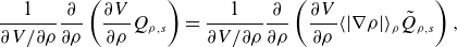 \begin{equation} \frac {1}{\partial V/\partial \rho }\frac {\partial }{\partial \rho }\left (\frac {\partial V}{\partial \rho } {Q_{\rho, s}} \right ) = \frac {1}{\partial V/\partial \rho }\frac {\partial }{\partial \rho } \left ( \frac {\partial V}{\partial \rho } \langle |\nabla \rho |\rangle _\rho \tilde {Q}_{\rho, s}\right ), \end{equation}
with $\tilde {Q}_{\rho, s} = Q_{\rho, s}/\langle |\nabla \rho |\rangle _\rho$
, consistent with our normalization defined in (3.1) (neglecting
$\tilde {Q}_{\rho, s} = Q_{\rho, s}/\langle |\nabla \rho |\rangle _\rho$
, consistent with our normalization defined in (3.1) (neglecting $Q_{GB}$
factors here). Additionally, note that the flux surface area satisfies
$Q_{GB}$
factors here). Additionally, note that the flux surface area satisfies $A_{{surf}} = (\partial V/\partial \psi ) \langle |\nabla \psi |\rangle _\psi$
for any arbitrary flux surface label
$A_{{surf}} = (\partial V/\partial \psi ) \langle |\nabla \psi |\rangle _\psi$
for any arbitrary flux surface label $\psi$
, including
$\psi$
, including $\rho$
. This means we can rewrite the divergence in terms of the arbitrary coordinate
$\rho$
. This means we can rewrite the divergence in terms of the arbitrary coordinate $\psi$
as
$\psi$
as
 \begin{equation} \frac {1}{\partial V/\partial \psi }\, \frac {\partial }{\partial \psi }\left (A_{{surf}}\, \tilde {Q}_{\rho, s}\right ), \end{equation}
which shows that with our normalization, the choice of the radial coordinate $\rho$
in the flux tube calculation can be made independent of the radial coordinate in the transport equation.
$\rho$
in the flux tube calculation can be made independent of the radial coordinate in the transport equation.
The turbulence is modelled by gyrokinetic calculations with GX, and the neoclassical transport is modelled with SFINCS (Landreman et al. Reference Landreman, Smith, Mollén and Helander2014) calculations. The net energy source includes sources from fusion alpha heating, auxiliary heating, collisional and turbulent energy exchange, and radiation losses (Bremsstrahlung, line, recombination, synchrotron). For Bremsstrahlung, line and recombination radiation we use cooling rates from Mavrin (Reference Mavrin2018). Details about the alpha heating model are given in the following subsection.
We assume a 50 : 50 deuterium–tritium-fuelled plasma with fuel dilution $f_{DT}=0.85$
, and a helium ash concentration
$f_{DT}=0.85$
, and a helium ash concentration $f_{He}=0.05$
. With tungsten planned as the material for the first wall, we include a tungsten concentration
$f_{He}=0.05$
. With tungsten planned as the material for the first wall, we include a tungsten concentration $f_W = 1.5\times 10^{-5}$
; we also include a low-Z radiator species in the form of a neon concentration
$f_W = 1.5\times 10^{-5}$
; we also include a low-Z radiator species in the form of a neon concentration $f_{Ne}=4.9\times 10^{-3}$
. The resulting effective ion charge is
$f_{Ne}=4.9\times 10^{-3}$
. The resulting effective ion charge is $Z_{{eff}}=1.62$
. These plasma composition assumptions are similar to assumptions used for SPARC transport analysis (Rodriguez-Fernandez et al. Reference Rodriguez-Fernandez, Howard, Greenwald, Creely, Hughes, Wright, Holland, Lin and Sciortino2020). While the average charge state for the tungsten ions in the anticipated temperature range is
$Z_{{eff}}=1.62$
. These plasma composition assumptions are similar to assumptions used for SPARC transport analysis (Rodriguez-Fernandez et al. Reference Rodriguez-Fernandez, Howard, Greenwald, Creely, Hughes, Wright, Holland, Lin and Sciortino2020). While the average charge state for the tungsten ions in the anticipated temperature range is $Z = 50\!-\!55$
, we have assumed nearly fully ionized (
$Z = 50\!-\!55$
, we have assumed nearly fully ionized ( $Z=72$
) tungsten ions; we believe this is a conservative assumption since it increases radiative losses from tungsten.
$Z=72$
) tungsten ions; we believe this is a conservative assumption since it increases radiative losses from tungsten.
The T3D solver discretizes the radial dimension using a finite volume scheme, and we use a coarse radial grid with six radial cells, centred at $\rho _{{grid}} = [0.15, 0.375, 0.525, 0.675, 0.8, 0.9]$
. The profile values at
$\rho _{{grid}} = [0.15, 0.375, 0.525, 0.675, 0.8, 0.9]$
. The profile values at $\rho _{BC}=0.9$
serve as the radial boundary condition for the transport equations and are thus held fixed throughout the calculation. Gyrokinetic and neoclassical fluxes are evaluated at cell interfaces, located at
$\rho _{BC}=0.9$
serve as the radial boundary condition for the transport equations and are thus held fixed throughout the calculation. Gyrokinetic and neoclassical fluxes are evaluated at cell interfaces, located at $\rho _{{flux}} = [0.3, 0.45, 0.6, 0.75, 0.85]$
. High-order spline interpolation is used to convert between the two grids and evaluate gradients. While the radial grid may seem coarse, the low magnetic shear configurations that we target have little radial variation in equilibrium quantities, and we do not expect sharp features such as internal transport barriers. Further discussion of the validity of coarse radial profiles in transport calculations can be found in Rodriguez-Fernandez et al. (Reference Rodriguez-Fernandez, Howard, Saltzman, Shoji, Body, Battaglia, Hughes, Candy, Staebler and Creely2024).
$\rho _{{flux}} = [0.3, 0.45, 0.6, 0.75, 0.85]$
. High-order spline interpolation is used to convert between the two grids and evaluate gradients. While the radial grid may seem coarse, the low magnetic shear configurations that we target have little radial variation in equilibrium quantities, and we do not expect sharp features such as internal transport barriers. Further discussion of the validity of coarse radial profiles in transport calculations can be found in Rodriguez-Fernandez et al. (Reference Rodriguez-Fernandez, Howard, Saltzman, Shoji, Body, Battaglia, Hughes, Candy, Staebler and Creely2024).
In all cases, we fix the boundary temperature to be $T_{BC} = T(\rho =0.9) = 2$
keV. This boundary condition is somewhat arbitrary as no physics-based model is mature enough to accurately predict the stellarator boundary plasma. One way to estimate the temperature at
$T_{BC} = T(\rho =0.9) = 2$
keV. This boundary condition is somewhat arbitrary as no physics-based model is mature enough to accurately predict the stellarator boundary plasma. One way to estimate the temperature at $\rho =0.9$
is to assume that the temperature follows gyroBohm scaling,
$\rho =0.9$
is to assume that the temperature follows gyroBohm scaling, $T(\rho =0.9) \sim C \,T_{GB} \sim C (a B^2 P / R n)^{0.4}$
. Assuming the same proportionality factor
$T(\rho =0.9) \sim C \,T_{GB} \sim C (a B^2 P / R n)^{0.4}$
. Assuming the same proportionality factor $C$
, we can use characteristic W7-X parameters (
$C$
, we can use characteristic W7-X parameters ( $a=0.5$
m,
$a=0.5$
m, $R=5.5$
m,
$R=5.5$
m, $B=2.5$
T,
$B=2.5$
T, $P=4$
MW,
$P=4$
MW, $n=0.6\times 10^{20}$
m
$n=0.6\times 10^{20}$
m $^{-3}$
), where
$^{-3}$
), where $T(\rho =0.9) \sim 0.3$
keV is a typical value (Beurskens et al. Reference Beurskens2021), to scale to Infinity Two parameters. For
$T(\rho =0.9) \sim 0.3$
keV is a typical value (Beurskens et al. Reference Beurskens2021), to scale to Infinity Two parameters. For $n=2\times 10^{20}$
m
$n=2\times 10^{20}$
m $^{-3}$
and
$^{-3}$
and $P\geqslant 100$
MW, we obtain
$P\geqslant 100$
MW, we obtain $T(\rho =0.9)\gtrsim 2$
keV. We note that this value is similar to boundary values used in modelling tokamak L-mode plasmas, which are reminiscent of this stellarator scenario, for the high-field SPARC tokamak (Rodriguez-Fernandez et al. Reference Rodriguez-Fernandez, Howard, Saltzman, Shoji, Body, Battaglia, Hughes, Candy, Staebler and Creely2024), and for the high-field power-plant-scale ARC concept (Frank et al. Reference Frank2022). Of course, near-edge transport may not scale like gyroBohm as boundary effects and atomic processes are likely to play an increasingly significant role. Our predictions of temperature profiles, confinement times and fusion performance will certainly vary with different chosen boundary temperature. Lower boundary temperature could degrade performance, while higher boundary temperature could affect pellet penetration and hence the achievable edge density gradient. A quantitative analysis of the sensitivity of our predictions to variations in the boundary temperature will be the subject of future analysis.
$T(\rho =0.9)\gtrsim 2$
keV. We note that this value is similar to boundary values used in modelling tokamak L-mode plasmas, which are reminiscent of this stellarator scenario, for the high-field SPARC tokamak (Rodriguez-Fernandez et al. Reference Rodriguez-Fernandez, Howard, Saltzman, Shoji, Body, Battaglia, Hughes, Candy, Staebler and Creely2024), and for the high-field power-plant-scale ARC concept (Frank et al. Reference Frank2022). Of course, near-edge transport may not scale like gyroBohm as boundary effects and atomic processes are likely to play an increasingly significant role. Our predictions of temperature profiles, confinement times and fusion performance will certainly vary with different chosen boundary temperature. Lower boundary temperature could degrade performance, while higher boundary temperature could affect pellet penetration and hence the achievable edge density gradient. A quantitative analysis of the sensitivity of our predictions to variations in the boundary temperature will be the subject of future analysis.
The profiles are time-advanced using an implicit second-order backward differencing scheme, which enables large time steps on transport time scales. In each time step, the nonlinear terms, which are the terms involving the heat and particle fluxes, are linearized using a multi-iteration Newton’s method. This algorithm can be used to evolve the profiles in time until a steady-state is reached where power and particle balance are satisfied.
While all six species are present in the T3D calculation, only the electron and deuterium temperature profiles are evolved self-consistently. The remaining ion temperature profiles are assumed to be equal to the deuterium temperature profile at each iteration. All source terms in the electron and deuterium evolution equations, including radiation and collisional equilibration, are computed using contributions from all six species. Note that only electron and deuterium heat fluxes are needed in order to evolve the electron and deuterium temperature profiles.
At each $\rho _{{flux}}$
radial location T3D runs several GX gyrokinetic calculations: one using the nominal gradients from the current profile state, and several more with perturbed gradients for each evolving profile, so that a Jacobian representing the sensitivity of fluxes to changes in gradients can be computed. The GX calculations are fully EM (including both perpendicular and compressional magnetic perturbations), include collisions with collision frequencies computed consistently with the local profile values at each iteration, include local variation of the equilibrium pressure gradient via the approach of Hegna & Nakajima (Reference Hegna and Nakajima1998) and are performed with the same numerical resolution as used in the scans in § 3. As noted above, only the electron and deuterium heat fluxes are needed for the transport calculation. While we could include all six kinetic species in the turbulence calculations and only use the heat fluxes from electrons and deuterium for transport, we choose to alleviate computational expense by reducing the GX calculations to only include deuterium and electrons, assuming no dilution and taking the deuterium–electron mass ratio. To account for the difference in species mix between GX (where we effectively assume
$\rho _{{flux}}$
radial location T3D runs several GX gyrokinetic calculations: one using the nominal gradients from the current profile state, and several more with perturbed gradients for each evolving profile, so that a Jacobian representing the sensitivity of fluxes to changes in gradients can be computed. The GX calculations are fully EM (including both perpendicular and compressional magnetic perturbations), include collisions with collision frequencies computed consistently with the local profile values at each iteration, include local variation of the equilibrium pressure gradient via the approach of Hegna & Nakajima (Reference Hegna and Nakajima1998) and are performed with the same numerical resolution as used in the scans in § 3. As noted above, only the electron and deuterium heat fluxes are needed for the transport calculation. While we could include all six kinetic species in the turbulence calculations and only use the heat fluxes from electrons and deuterium for transport, we choose to alleviate computational expense by reducing the GX calculations to only include deuterium and electrons, assuming no dilution and taking the deuterium–electron mass ratio. To account for the difference in species mix between GX (where we effectively assume $n_{e,GX}=n_D$
, as required by quasineutrality) and T3D (where
$n_{e,GX}=n_D$
, as required by quasineutrality) and T3D (where $n_e = n_D/0.425$
), we must scale the normalized electron heat flux from GX up by a factor of
$n_e = n_D/0.425$
), we must scale the normalized electron heat flux from GX up by a factor of $(n_e/n_{e,GX})= 1/0.425\approx 2.35$
in the T3D calculation. No scaling is required for the deuterium heat flux because deuterium is treated as the reference species in both T3D and GX. Note that the simplification of neglecting impurities could make the transport calculations somewhat conservative, as the inclusion of impurities and fuel dilution has been shown to have a stabilizing effect on ITG turbulence (Rodriguez-Fernandez et al. Reference Rodriguez-Fernandez, Howard, Saltzman, Shoji, Body, Battaglia, Hughes, Candy, Staebler and Creely2024; García-Regaña et al. Reference García-Regaña, Calvo, Parra and Thienpondt2024). We provide a limited investigation of impurity effects in § 4.4.
$(n_e/n_{e,GX})= 1/0.425\approx 2.35$
in the T3D calculation. No scaling is required for the deuterium heat flux because deuterium is treated as the reference species in both T3D and GX. Note that the simplification of neglecting impurities could make the transport calculations somewhat conservative, as the inclusion of impurities and fuel dilution has been shown to have a stabilizing effect on ITG turbulence (Rodriguez-Fernandez et al. Reference Rodriguez-Fernandez, Howard, Saltzman, Shoji, Body, Battaglia, Hughes, Candy, Staebler and Creely2024; García-Regaña et al. Reference García-Regaña, Calvo, Parra and Thienpondt2024). We provide a limited investigation of impurity effects in § 4.4.
Similarly, several radially local SFINCS neoclassical transport calculations are run at each $\rho _{{flux}}$
location. In each of these calculations a Brent root-finding algorithm is used to solve for the ambipolar radial electric field. The computed particle and heat fluxes from the ambipolar state are then passed to T3D. In the SFINCS calculations we include all six kinetic species, but as noted above only the electron and deuterium heat fluxes are used in the transport calculation.
$\rho _{{flux}}$
location. In each of these calculations a Brent root-finding algorithm is used to solve for the ambipolar radial electric field. The computed particle and heat fluxes from the ambipolar state are then passed to T3D. In the SFINCS calculations we include all six kinetic species, but as noted above only the electron and deuterium heat fluxes are used in the transport calculation.
4.2. Heating and fuelling models
The two heating sources considered for this study are the thermalization of deuterium–tritium fusion generated alpha particles born at 3.5 MeV, and externally applied ECRH. We use deuterium–tritium cross-sections from the ENDF nuclear reaction database (Brown et al. Reference Brown2018), and we use a model based on the classical slowing down distribution to evaluate alpha thermalization to electrons and the lumped ion species (Stix Reference Stix1972). We assume an alpha heating efficiency of $k_\alpha =0.9$
to account for alpha particle losses before thermalization due to drift orbits or Alfvenic activity. This is likely a conservative assumption based on the
$k_\alpha =0.9$
to account for alpha particle losses before thermalization due to drift orbits or Alfvenic activity. This is likely a conservative assumption based on the $\lt 4\,\%$ $\alpha$
energy losses simulated for this configuration (Carbajal et al. Reference Carbajal2025).
$\alpha$
energy losses simulated for this configuration (Carbajal et al. Reference Carbajal2025).
We choose to use ECRH heating, assuming the availability of 236 GHz gyrotrons with fundamental resonance at 8.42 T (Thumm et al. Reference Thumm, Denisov, Sakamoto and Tran2019; Jelonnek et al. Reference Jelonnek2017). A perpendicular launch angle is assumed to minimize any potential current drive. While there is an assumed strong density gradient, the cutoff density for the O1 heating scheme is $\sim 7\times 10^{20}\ {\rm m}^{-3}$
so refraction effects are expected to be insignificant. Very high first pass absorption is expected at the large central electron temperatures of 15 keV (Westerhof Reference Westerhof2010). The beam width will be a few centimetres, much smaller than the vertical cross-section. Altogether, a very narrow absorption width is expected. Therefore, when ECRH heating is used in the transport predictions we assume a Gaussian profile centred at
$\sim 7\times 10^{20}\ {\rm m}^{-3}$
so refraction effects are expected to be insignificant. Very high first pass absorption is expected at the large central electron temperatures of 15 keV (Westerhof Reference Westerhof2010). The beam width will be a few centimetres, much smaller than the vertical cross-section. Altogether, a very narrow absorption width is expected. Therefore, when ECRH heating is used in the transport predictions we assume a Gaussian profile centred at $\rho$
= 0.1 with a width
$\rho$
= 0.1 with a width $\sigma$
= 0.05. Note that even when targeting ignition conditions (
$\sigma$
= 0.05. Note that even when targeting ignition conditions ( $P_{{aux}}=0$
) for the operating point, auxiliary heating will be required to access and control fusion burn.
$P_{{aux}}=0$
) for the operating point, auxiliary heating will be required to access and control fusion burn.
In this work we predict only temperature profiles, so a density profile must be assumed. We use the form described in § 3 that is flat in the core and has increasing gradient outside $\rho \gt 0.6$
in the region where pellet fuelling is expected. To assess the credibility of this assumption, NGS equations are used to compute the pellet mass ablation rate from which a fuelling profile is derived assuming point deposition. Drift homogenization of the ablated pellet mass, which can act favourably to increase the pellet penetration depth (Geulin & Pégourié Reference Geulin and Pégourié2022), is neglected. We adopt the model in McClenaghan et al. (Reference McClenaghan, Lao, Parks, Wu, Zhang and Chan2023) and Zhang & Parks (Reference Zhang and Parks2020), where the ablation rate is given by
$\rho \gt 0.6$
in the region where pellet fuelling is expected. To assess the credibility of this assumption, NGS equations are used to compute the pellet mass ablation rate from which a fuelling profile is derived assuming point deposition. Drift homogenization of the ablated pellet mass, which can act favourably to increase the pellet penetration depth (Geulin & Pégourié Reference Geulin and Pégourié2022), is neglected. We adopt the model in McClenaghan et al. (Reference McClenaghan, Lao, Parks, Wu, Zhang and Chan2023) and Zhang & Parks (Reference Zhang and Parks2020), where the ablation rate is given by
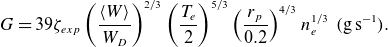 \begin{align} G = 39 \zeta _{{exp}} \left ( \frac {\left \lt W\right \gt }{W_D}\right )^{2/3} \left ( \frac {T_{e}}{2}\right )^{5/3} \left (\frac {r_p}{0.2}\right )^{4/3} n_{e}^{1/3}\;\;\mathrm {(g\,s^{-1})}. \end{align}
The mean molar mass $\left \lt W\right \gt$
is taken as the weighted average of the molar mass of deuterium (
$\left \lt W\right \gt$
is taken as the weighted average of the molar mass of deuterium ( $W_D$
) and tritium (
$W_D$
) and tritium ( $W_T$
). The extra factor
$W_T$
). The extra factor $\zeta _{{exp}} = (2/B_T)^{0.843}$
includes a magnetic field dependence to capture the decreasing ablation rate due to plasma shielding effects. There is uncertainty in the exponent in this expression, with McClenaghan et al. (Reference McClenaghan, Lao, Parks, Wu, Zhang and Chan2023) and Zhang & Parks (Reference Zhang and Parks2020) choosing values of (0.843, 0.6, 0.35) derived from fits to various published ablation simulations.
$\zeta _{{exp}} = (2/B_T)^{0.843}$
includes a magnetic field dependence to capture the decreasing ablation rate due to plasma shielding effects. There is uncertainty in the exponent in this expression, with McClenaghan et al. (Reference McClenaghan, Lao, Parks, Wu, Zhang and Chan2023) and Zhang & Parks (Reference Zhang and Parks2020) choosing values of (0.843, 0.6, 0.35) derived from fits to various published ablation simulations.
Fuelling profiles computed using the NGS model for bracketing values of initial pellet radius and velocity. The rate of pellet injection has been adjusted so that the integrated sources are equal for the two pellet sizes. The inset shows path of pellet injection trajectory from the outboard $\phi$
= 0 cross-section up to
$\phi$
= 0 cross-section up to $\rho =0.65$
.
$\rho =0.65$
.
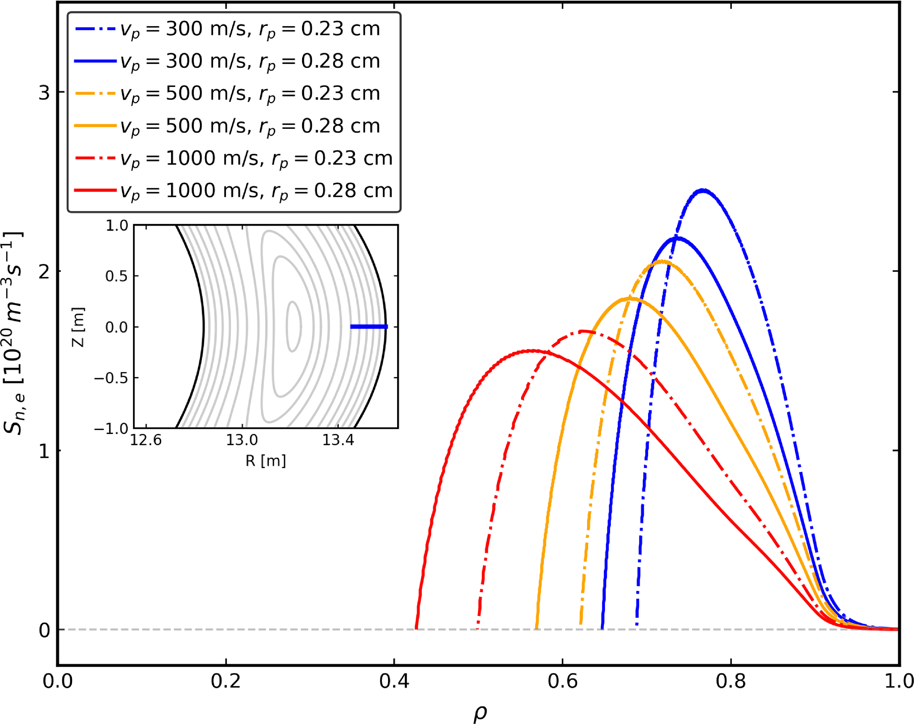
Assuming spherical pellets comprised of an equal mix of deuterium and tritium, calculations are performed using pellet velocities, $v_p$
= 300–500 ms−1, and radii,
$v_p$
= 300–500 ms−1, and radii, $r_p$
= 0.23–0.28 cm, bracketing the anticipated ranges for ITER fuelling injectors (Baylor et al. Reference Baylor, Parks, Jernigan, Caughman, Combs, Foust, Houlberg, Maruyama and Rasmussen2007). An additional set of simulations is done for
$r_p$
= 0.23–0.28 cm, bracketing the anticipated ranges for ITER fuelling injectors (Baylor et al. Reference Baylor, Parks, Jernigan, Caughman, Combs, Foust, Houlberg, Maruyama and Rasmussen2007). An additional set of simulations is done for $v_p$
= 1000 ms−1, representative of the higher range tested with the W7-X continuous pellet fuelling system (Meitner & Baylor Reference Meitner and Baylor2023). The frequency of pellet injection for the two pellet sizes is set to 4 Hz (2.2 Hz) for
$v_p$
= 1000 ms−1, representative of the higher range tested with the W7-X continuous pellet fuelling system (Meitner & Baylor Reference Meitner and Baylor2023). The frequency of pellet injection for the two pellet sizes is set to 4 Hz (2.2 Hz) for $r_p$
= 0.23 cm (0.28 cm) to provide the same time-averaged fuelling rate based on simulations below,
$r_p$
= 0.23 cm (0.28 cm) to provide the same time-averaged fuelling rate based on simulations below, $S_{fuel}=2.2\times 10^{22}$
s
$S_{fuel}=2.2\times 10^{22}$
s $^{-1}$
. The number of injected particles per pellet (
$^{-1}$
. The number of injected particles per pellet ( $0.62, 1.1 \times 10^{21}$
) is less than 5 % of the total plasma inventory for these choices (depending on
$0.62, 1.1 \times 10^{21}$
) is less than 5 % of the total plasma inventory for these choices (depending on $\langle n \rangle$
), so that transient cooling effects should be minimal. Injection is prescribed to be from the outboard midplane at the narrowest bean-shaped
$\langle n \rangle$
), so that transient cooling effects should be minimal. Injection is prescribed to be from the outboard midplane at the narrowest bean-shaped $\phi =0$
plane where deposition without drifts should be deepest. Electron density and temperature profiles for these calculations come from the profile predictions shown below, but are nearly identical to calculations using the initial assumed profiles. As shown in figure 8, the pellets are predicted to penetrate into
$\phi =0$
plane where deposition without drifts should be deepest. Electron density and temperature profiles for these calculations come from the profile predictions shown below, but are nearly identical to calculations using the initial assumed profiles. As shown in figure 8, the pellets are predicted to penetrate into $\rho$
= 0.43–0.7 with electron source rate profiles peaking between
$\rho$
= 0.43–0.7 with electron source rate profiles peaking between $\rho$
= 0.58–0.8. These profiles indicate it should be plausible to enhance edge density gradients in the outer 40–50 % of the radial profile. There are many uncertainties in these calculations; e.g. if a weaker dependence of
$\rho$
= 0.58–0.8. These profiles indicate it should be plausible to enhance edge density gradients in the outer 40–50 % of the radial profile. There are many uncertainties in these calculations; e.g. if a weaker dependence of $\zeta _{{exp}} = (2/B_T)^{0.35}$
is assumed, the penetration depth is shifted outward up to
$\zeta _{{exp}} = (2/B_T)^{0.35}$
is assumed, the penetration depth is shifted outward up to $\Delta \rho \approx 0.1$
. On the other hand, drift homogenization (not accounted for here) can further reduce or enhance penetration depending on injection geometry with respect to expected drift effects (Panadero et al. Reference Panadero2018). More sophisticated calculations are being pursued to better quantify these effects.
$\Delta \rho \approx 0.1$
. On the other hand, drift homogenization (not accounted for here) can further reduce or enhance penetration depending on injection geometry with respect to expected drift effects (Panadero et al. Reference Panadero2018). More sophisticated calculations are being pursued to better quantify these effects.
Parameters from T3D-GX-SFINCS temperature profile predictions.
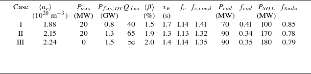
Assumed density profiles (a) and predicted temperature (b) and total $\beta$
(c) profiles from T3D, along with normalized inverse density (d) and temperature (e) gradient scale lengths and pressure gradient
$\beta$
(c) profiles from T3D, along with normalized inverse density (d) and temperature (e) gradient scale lengths and pressure gradient $-\beta '=-d\beta /d\rho _{{tor}}$
(f). In (e) the
$-\beta '=-d\beta /d\rho _{{tor}}$
(f). In (e) the $\eta _i=L_n/L_{Ti}=1$
profile (dotted) shows that the temperature gradients at the outer radii lie near the
$\eta _i=L_n/L_{Ti}=1$
profile (dotted) shows that the temperature gradients at the outer radii lie near the $\eta _i=1$
threshold. In (f) we also plot the IBM linear instability threshold estimate (dotted), which was computed as described in § 3.1 using the preliminary assumed pressure profiles.
$\eta _i=1$
threshold. In (f) we also plot the IBM linear instability threshold estimate (dotted), which was computed as described in § 3.1 using the preliminary assumed pressure profiles.
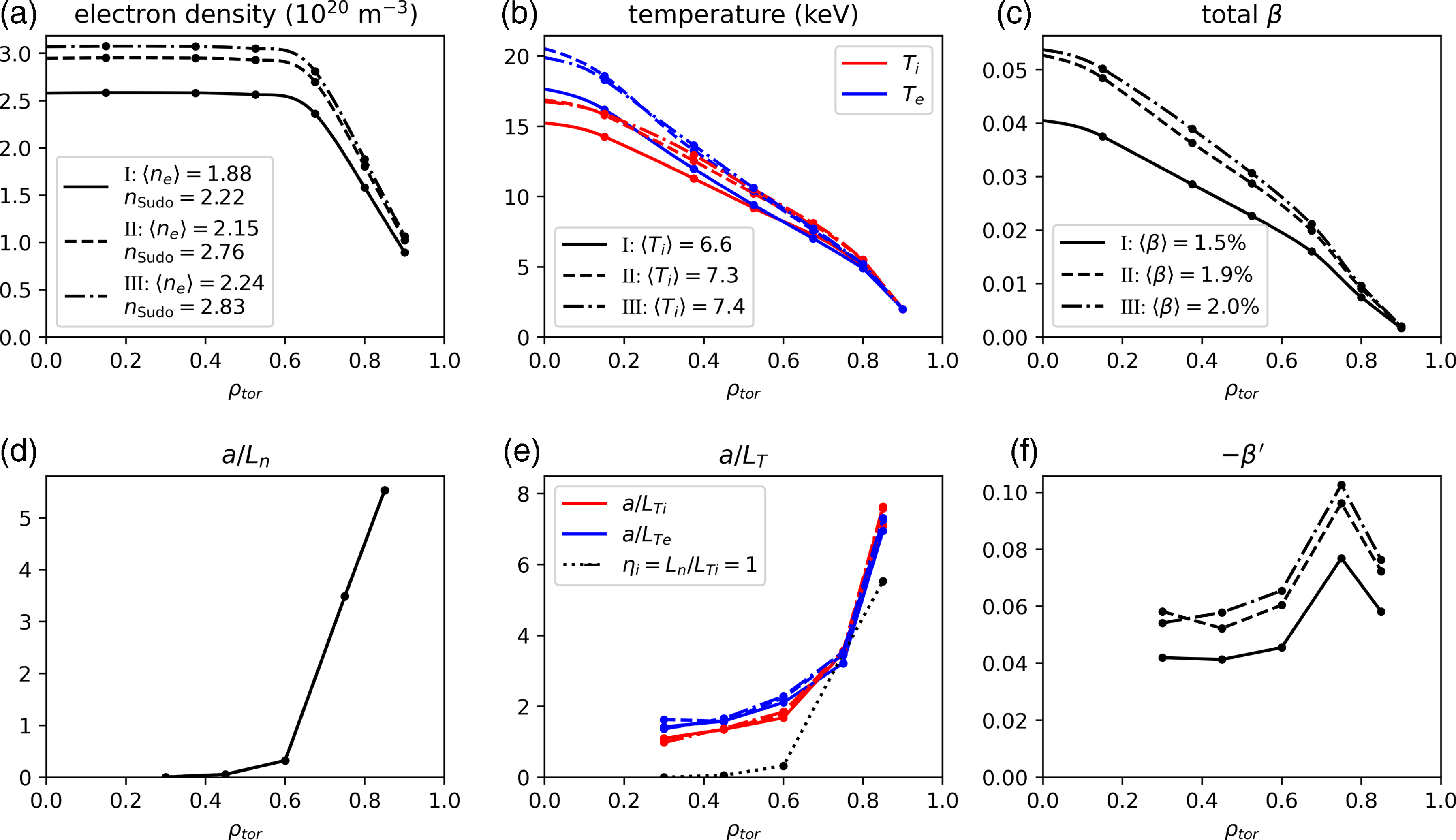
4.3. Temperature profile predictions
We present three cases at different volume-averaged density, with the results summarized in table 5 and profiles plotted in figure 9. In each case the electron and ion temperature profiles are predicted, with the edge temperature at $\rho _{BC}=0.9$
fixed at
$\rho _{BC}=0.9$
fixed at $T_{BC}=2$
keV as discussed above. In the lowest density case (Case I) with
$T_{BC}=2$
keV as discussed above. In the lowest density case (Case I) with $\langle n_e\rangle = 1.88\times 10^{20}$
m
$\langle n_e\rangle = 1.88\times 10^{20}$
m $^{-3}$
, auxiliary heating of
$^{-3}$
, auxiliary heating of $P_{{aux}}=20$
MW is applied to the electrons on-axis. This case produces
$P_{{aux}}=20$
MW is applied to the electrons on-axis. This case produces $P_{{fus,DT}}=800$
MW (
$P_{{fus,DT}}=800$
MW ( $Q_{{fus}}=40$
). In Case II, the density is increased by 15 % to
$Q_{{fus}}=40$
). In Case II, the density is increased by 15 % to $\langle n_e\rangle = 2.15\times 10^{20}$
m
$\langle n_e\rangle = 2.15\times 10^{20}$
m $^{-3}$
while maintaining
$^{-3}$
while maintaining $P_{{aux}}=20$
MW, resulting in
$P_{{aux}}=20$
MW, resulting in $P_{{fus,DT}}=1.3$
GW (
$P_{{fus,DT}}=1.3$
GW ( $Q_{{fus}}=65$
). In Case III we increase the density an additional 5 % to
$Q_{{fus}}=65$
). In Case III we increase the density an additional 5 % to $\langle n_e\rangle = 2.24\times 10^{20}$
m
$\langle n_e\rangle = 2.24\times 10^{20}$
m $^{-3}$
and remove the auxiliary heating to achieve an ignited (
$^{-3}$
and remove the auxiliary heating to achieve an ignited ( $Q_{{fus}}=\infty$
) operating point at
$Q_{{fus}}=\infty$
) operating point at $P_{{fus,DT}}=1.5$
GW. In each case the volume-averaged density (as well as the line-average density) is less than the Sudo density; the edge density is far below
$P_{{fus,DT}}=1.5$
GW. In each case the volume-averaged density (as well as the line-average density) is less than the Sudo density; the edge density is far below $0.8 n_{{Sudo}}$
, which has been shown to be a more relevant limit for pellet-fuelled discharges with peaked density profiles on LHD (Miyazawa et al. Reference Miyazawa2008b
).
$0.8 n_{{Sudo}}$
, which has been shown to be a more relevant limit for pellet-fuelled discharges with peaked density profiles on LHD (Miyazawa et al. Reference Miyazawa2008b
).
(a) Heating sources from fusion alphas (solid) and auxiliary ECRH heating (dashed), (b) energy exchange between species due to collisions (solid) and turbulent heating (dashed) and (c) radiation losses for Case I. The total radiated power in this case is $P_{{rad}}\approx 70$
MW (
$P_{{rad}}\approx 70$
MW ( $f_{{rad}}=0.41$
), with the radiation profile shown by the solid blue line in (c). The contributions from Bremsstrahlung (black), line and recombination (cyan) and synchrotron (green) radiation are shown with dotted lines. The dashed lines show a breakdown of the sum of the Bremsstrahlung, line and recombination radiation by impurity species: helium (pink); tungsten (purple); neon (brown).
$f_{{rad}}=0.41$
), with the radiation profile shown by the solid blue line in (c). The contributions from Bremsstrahlung (black), line and recombination (cyan) and synchrotron (green) radiation are shown with dotted lines. The dashed lines show a breakdown of the sum of the Bremsstrahlung, line and recombination radiation by impurity species: helium (pink); tungsten (purple); neon (brown).

Examining the predicted temperature profiles and gradients (figures 9
b and 9
e), we find the ions and electrons are well equilibrated ( $T_i \sim T_e$
) for
$T_i \sim T_e$
) for $\rho \gtrsim 0.6$
in each case. The on-axis temperature ratio is
$\rho \gtrsim 0.6$
in each case. The on-axis temperature ratio is $T_{e0}/T_{i0}\approx 1.2$
for all cases. The normalized temperature gradients are very similar in all cases, with small increases in
$T_{e0}/T_{i0}\approx 1.2$
for all cases. The normalized temperature gradients are very similar in all cases, with small increases in $a/L_T$
at the outer radii leading to raised temperature profiles in Cases II and III compared with Case I. This self-similarity between the temperature profiles at different density (and power) operating points is an indication of the stiff transport that sets the profile gradients. The temperature gradients are strong in the region of large density gradient, consistent with density gradient stabilization of ITG turbulence as discussed in § 3, and as indicated with the
$a/L_T$
at the outer radii leading to raised temperature profiles in Cases II and III compared with Case I. This self-similarity between the temperature profiles at different density (and power) operating points is an indication of the stiff transport that sets the profile gradients. The temperature gradients are strong in the region of large density gradient, consistent with density gradient stabilization of ITG turbulence as discussed in § 3, and as indicated with the $\eta _i=1$
curve in figure 9(e).
$\eta _i=1$
curve in figure 9(e).
Table 5 also shows the predicted energy confinement time for each case, $\tau _E = W/P_{{heat}}$
and the confinement factor
$\tau _E = W/P_{{heat}}$
and the confinement factor $f_c = \tau _E/\tau _{{ISS04}}$
, with
$f_c = \tau _E/\tau _{{ISS04}}$
, with $P_{{heat}} = P_{{aux}} + P_\alpha$
. All three cases achieve
$P_{{heat}} = P_{{aux}} + P_\alpha$
. All three cases achieve $f_c \approx 1.13-1.14$
. Note that the ISS04 scaling is not strictly valid for cases with significant radiated power. If we subtract radiation losses from fusion and alpha heating to get the net heating power
$f_c \approx 1.13-1.14$
. Note that the ISS04 scaling is not strictly valid for cases with significant radiated power. If we subtract radiation losses from fusion and alpha heating to get the net heating power $P_{{heat,net}} = P_{{aux}} + P_\alpha - P_{{rad}}$
, we can use this to compute the conductive energy confinement time as
$P_{{heat,net}} = P_{{aux}} + P_\alpha - P_{{rad}}$
, we can use this to compute the conductive energy confinement time as $\tau _{E,{cond}}=\tau _E/(1-f_{{rad}})$
; using the same net heating power in the ISS04 scaling (
$\tau _{E,{cond}}=\tau _E/(1-f_{{rad}})$
; using the same net heating power in the ISS04 scaling ( $\tau _{{ISS04}}\sim P_{{heat}}^{-0.61}$
, so
$\tau _{{ISS04}}\sim P_{{heat}}^{-0.61}$
, so $\tau _{{ISS04,cond}}\sim \tau _{{ISS04}}(1-f_{{rad}})^{-0.61}$
), we obtain
$\tau _{{ISS04,cond}}\sim \tau _{{ISS04}}(1-f_{{rad}})^{-0.61}$
), we obtain $f_{c,{cond}}=\tau _{E,{cond}}/\tau _{{ISS04, cond}} = f_c (1-f_{{rad}})^{-0.39}$
. The conductive energy confinement time effectively measures how quickly energy is conducted and lost solely due to transport processes (turbulence and neoclassical transport), and thus is perhaps more representative of the transport optimization that we are targeting. All cases achieve
$f_{c,{cond}}=\tau _{E,{cond}}/\tau _{{ISS04, cond}} = f_c (1-f_{{rad}})^{-0.39}$
. The conductive energy confinement time effectively measures how quickly energy is conducted and lost solely due to transport processes (turbulence and neoclassical transport), and thus is perhaps more representative of the transport optimization that we are targeting. All cases achieve $f_{c,{cond}}\approx 1.3-1.4$
. We note that any variation in the boundary temperature, held fixed here, with varying power and density will cause additional variation in the inferred confinement factor due to the stiff transport discussed above; this will be a subject of future investigation.
$f_{c,{cond}}\approx 1.3-1.4$
. We note that any variation in the boundary temperature, held fixed here, with varying power and density will cause additional variation in the inferred confinement factor due to the stiff transport discussed above; this will be a subject of future investigation.
Profiles of the heating sources, radiation sinks and collisional and turbulent exchange terms for Case I are shown in figure 10. The calculation of the fusion power includes contributions from all of the energetic alpha particles and neutrons resulting from deuterium–tritium reactions, but we (conservatively) do not account for exothermic neutron–lithium reactions in the breeder as has been included in other power plant studies (Alonso et al. Reference Alonso, Calvo, Carralero, Velasco, García-Regaña, Palermo and Rapisarda2022). The value of $P_\alpha$
includes the assumed 90 % thermalization efficiency, but the lost alpha power is recovered in the total deuterium–tritium fusion power so that
$P_\alpha$
includes the assumed 90 % thermalization efficiency, but the lost alpha power is recovered in the total deuterium–tritium fusion power so that $P_{{fus}} = 5.03(P_\alpha /0.9)$
. According to the alpha thermalization model, 80 % of the alpha heating goes to the electrons. Approximately 70 MW of power is radiated, primarily by the tungsten and neon impurities, with Bremsstrahlung providing the largest contribution. This leaves roughly 100 MW of power flow into the periphery. Large edge line radiation will not be accurately represented until lower temperatures and increased impurity fractions in the outer 10 % of the minor radius are included in the simulation. In the inner core region
$P_{{fus}} = 5.03(P_\alpha /0.9)$
. According to the alpha thermalization model, 80 % of the alpha heating goes to the electrons. Approximately 70 MW of power is radiated, primarily by the tungsten and neon impurities, with Bremsstrahlung providing the largest contribution. This leaves roughly 100 MW of power flow into the periphery. Large edge line radiation will not be accurately represented until lower temperatures and increased impurity fractions in the outer 10 % of the minor radius are included in the simulation. In the inner core region $\rho \leqslant 0.6$
where
$\rho \leqslant 0.6$
where $T_e\gt T_i$
, the electrons transfer roughly 25 MW to the ions via collisional energy exchange, as shown in figure 10(b). For
$T_e\gt T_i$
, the electrons transfer roughly 25 MW to the ions via collisional energy exchange, as shown in figure 10(b). For $\rho \gt 0.6$
, the ion temperature is slightly higher than the electron temperature, resulting in approximately 13 MW transferred from the ions to the electrons. This is an indication that the collisional exchange time is comparable to the energy confinement time at these large densities and modest temperatures, allowing for relatively efficient equilibration of the thermal ions and electrons. This alleviates concerns that the optimized turbulence conditions will be degraded by excessively large values of
$\rho \gt 0.6$
, the ion temperature is slightly higher than the electron temperature, resulting in approximately 13 MW transferred from the ions to the electrons. This is an indication that the collisional exchange time is comparable to the energy confinement time at these large densities and modest temperatures, allowing for relatively efficient equilibration of the thermal ions and electrons. This alleviates concerns that the optimized turbulence conditions will be degraded by excessively large values of $T_e/T_i$
. Cases II and III exhibit similar source and sink profiles, with the exception that no auxiliary heating is included in Case III, resulting in less collisional energy exchange due to lower
$T_e/T_i$
. Cases II and III exhibit similar source and sink profiles, with the exception that no auxiliary heating is included in Case III, resulting in less collisional energy exchange due to lower $T_e/T_i$
.
$T_e/T_i$
.
(a) Power balance for electrons (blue) and bulk D–T ions (red) in MW for Case I. Solid lines with open markers denote turbulent (diamonds), neoclassical (squares) and total (circles) fluxes. The volume integrated sources (composed of the terms plotted in figure 10) are shown with dotted lines with closed circle markers. (b) The a posteriori particle balance assessment, comparing the particle fluxes (open circles, dominated by turbulence) with integrated pellet source profiles with several assumptions about the pellet radius ( $r_p$
) and velocity (
$r_p$
) and velocity ( $v_p$
).
$v_p$
).
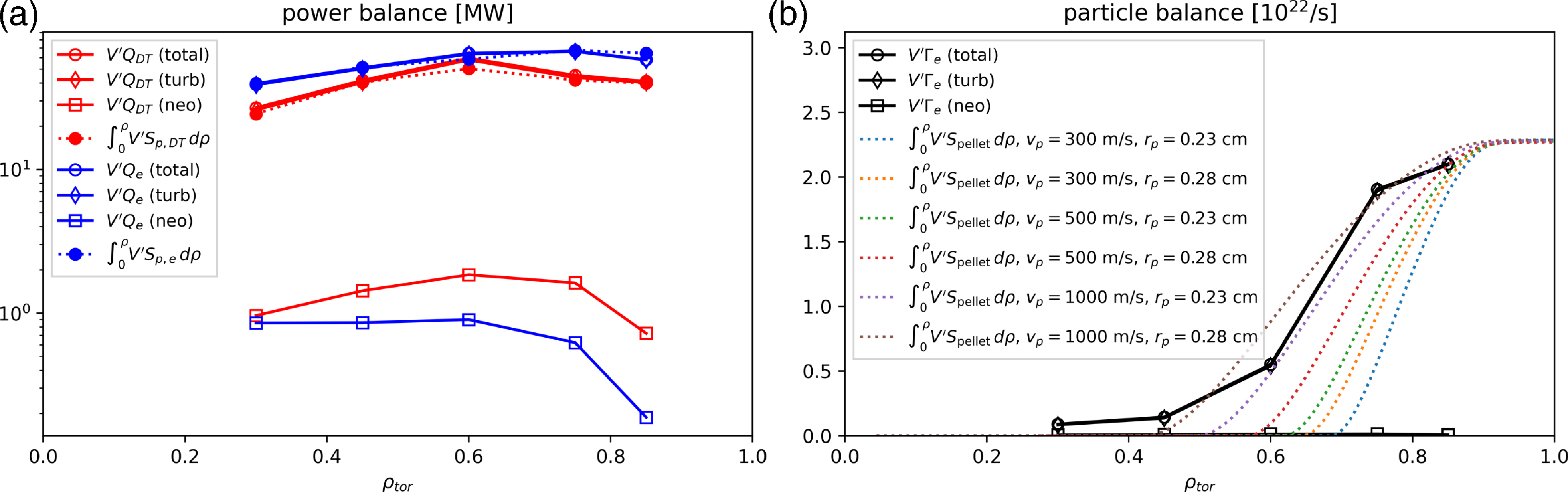
The converged steady-state profiles are achieved when the system reaches power balance, such that the heat flux at each radius matches the integrated source power (composed of the terms plotted in figure 10) interior to that radius. Integrating equation (4.1) over the volume contained within the flux surface labelled $\rho$
, and taking the steady-state (
$\rho$
, and taking the steady-state ( $\partial /\partial t\rightarrow 0$
) limit, this takes the form
$\partial /\partial t\rightarrow 0$
) limit, this takes the form
 \begin{equation} V' Q_{\rho, s} = \int _0^\rho V'\, S_{p,s}\, {d}\rho, \end{equation}
where $S_{p,s}$
denotes the right-hand side of (4.1) for species
$S_{p,s}$
denotes the right-hand side of (4.1) for species $s$
. Again focusing on Case I, this is shown in figure 11(a) by comparing the total fluxes (open circles with solid lines) with the integrated sources (closed circles with dotted lines) for both deuterium–tritium ions (red) and electrons (blue). The combined deuterium–tritium ion heat flux has been estimated by doubling the computed deuterium heat flux, and similarly for the deuterium–tritium sources. Separate transport contributions from turbulence (diamonds) and neoclassical (squares) are also shown. The turbulent transport contributions are more than 10
$s$
. Again focusing on Case I, this is shown in figure 11(a) by comparing the total fluxes (open circles with solid lines) with the integrated sources (closed circles with dotted lines) for both deuterium–tritium ions (red) and electrons (blue). The combined deuterium–tritium ion heat flux has been estimated by doubling the computed deuterium heat flux, and similarly for the deuterium–tritium sources. Separate transport contributions from turbulence (diamonds) and neoclassical (squares) are also shown. The turbulent transport contributions are more than 10 $\times$
larger than the neoclassical contributions everywhere for the ions, which is an indication of successful neoclassical optimization.
$\times$
larger than the neoclassical contributions everywhere for the ions, which is an indication of successful neoclassical optimization.
We also make an a posteriori assessment of particle balance in figure 11(b) by comparing the computed electron (and main ion) particle fluxes with the integrated pellet source profiles from the pellet model described above with various assumptions about the pellet radius ( $r_p$
) and velocity (
$r_p$
) and velocity ( $v_p$
). From this analysis it is seen that a pellet injection velocity of
$v_p$
). From this analysis it is seen that a pellet injection velocity of $v_p\sim 1000$
ms-1 should ensure sufficient penetration to sustain an edge density profile gradient very close to the assumed shape. These pellet velocities have been demonstrated with existing technology via the W7-X continuous pellet fuelling system (Meitner & Baylor Reference Meitner and Baylor2023). The required fuelling rate scales roughly with the density, so for Case III the pellet fuelling rate would need to be
$v_p\sim 1000$
ms-1 should ensure sufficient penetration to sustain an edge density profile gradient very close to the assumed shape. These pellet velocities have been demonstrated with existing technology via the W7-X continuous pellet fuelling system (Meitner & Baylor Reference Meitner and Baylor2023). The required fuelling rate scales roughly with the density, so for Case III the pellet fuelling rate would need to be $\sim 25\,\%$
higher, which is still within acceptable operational limits. The ability to sustain sufficient edge gradient will also depend on the density at the boundary that can be sustained by exhaust and pumping characteristics, but we assume it will be maintained below the Sudo density to avoid radiative collapse. In the inner core where no pellet fuelling is predicted, a small hollowing of the density profile would occur in this configuration as no source exists to balance the outward transport of particle fluxes, consistent with the analysis in § 3. The self-consistent prediction of density and fuelling profiles are required to confirm the above expectations, and is the subject of ongoing analysis.
$\sim 25\,\%$
higher, which is still within acceptable operational limits. The ability to sustain sufficient edge gradient will also depend on the density at the boundary that can be sustained by exhaust and pumping characteristics, but we assume it will be maintained below the Sudo density to avoid radiative collapse. In the inner core where no pellet fuelling is predicted, a small hollowing of the density profile would occur in this configuration as no source exists to balance the outward transport of particle fluxes, consistent with the analysis in § 3. The self-consistent prediction of density and fuelling profiles are required to confirm the above expectations, and is the subject of ongoing analysis.
To verify the key transport features discussed in § 3, in figure 12 we inspect the deuterium–tritium heat fluxes as a function of $a/L_{Ti}$
and
$a/L_{Ti}$
and $\beta '$
from the large number of GX simulations computed throughout the T3D iterations. Here we show the deuterium–tritium fluxes normalized to the deuterium gyroBohm heat flux,
$\beta '$
from the large number of GX simulations computed throughout the T3D iterations. Here we show the deuterium–tritium fluxes normalized to the deuterium gyroBohm heat flux, $Q_{D,GB} = n_D T_D v_{t,D}\rho _D^2 /a^2$
, and we again estimate the combined deuterium–tritium heat flux by scaling up the deuterium fluxes computed by GX by a factor of 2. The colours distinguish the radii where fluxes are computed, while the marker shapes denote the three cases with varying volume-averaged density. The black marker in each cluster denotes the final values computed using the converged profiles. While we only show the normalized ion heat flux here, we note that
$Q_{D,GB} = n_D T_D v_{t,D}\rho _D^2 /a^2$
, and we again estimate the combined deuterium–tritium heat flux by scaling up the deuterium fluxes computed by GX by a factor of 2. The colours distinguish the radii where fluxes are computed, while the marker shapes denote the three cases with varying volume-averaged density. The black marker in each cluster denotes the final values computed using the converged profiles. While we only show the normalized ion heat flux here, we note that $Q_e/Q_{DT}\sim 1-2$
in almost all cases, and
$Q_e/Q_{DT}\sim 1-2$
in almost all cases, and $\chi _e/\chi _{DT}\sim (Q_e/Q_{DT})(n_e/n_{DT})\lesssim 1$
at the inner radii where the weak density gradient results in ITG behaviour, and
$\chi _e/\chi _{DT}\sim (Q_e/Q_{DT})(n_e/n_{DT})\lesssim 1$
at the inner radii where the weak density gradient results in ITG behaviour, and $\chi _e/\chi _{DT}\sim 1-2$
at the outer radii where the behaviour is TEM-like. Over the limited range of
$\chi _e/\chi _{DT}\sim 1-2$
at the outer radii where the behaviour is TEM-like. Over the limited range of $a/L_{Ti}$
values evaluated for each radius, the
$a/L_{Ti}$
values evaluated for each radius, the $Q_{DT}-a/L_{Ti}$
relationships appear to be quite steep, an indication of stiff transport. At the three inner radii where the density gradients are small, extrapolating the data linearly to
$Q_{DT}-a/L_{Ti}$
relationships appear to be quite steep, an indication of stiff transport. At the three inner radii where the density gradients are small, extrapolating the data linearly to $Q_{DT}=0$
would give an effective threshold
$Q_{DT}=0$
would give an effective threshold $a/L_{Ti,crit} \approx$
1–1.5. At the outer radii, the threshold gradient appears to be higher due to the larger density gradients at these radii. Particularly for
$a/L_{Ti,crit} \approx$
1–1.5. At the outer radii, the threshold gradient appears to be higher due to the larger density gradients at these radii. Particularly for $\rho =0.85$
, the fluxes for the higher density cases (Cases II and III) are upshifted to larger
$\rho =0.85$
, the fluxes for the higher density cases (Cases II and III) are upshifted to larger $a/L_{Ti}$
, which is an indication of EM stabilization of the ITG turbulence, consistent with the results shown in figure 5. This upshift leads to increased temperature gradients at
$a/L_{Ti}$
, which is an indication of EM stabilization of the ITG turbulence, consistent with the results shown in figure 5. This upshift leads to increased temperature gradients at $\rho =0.85$
and consequent raised temperature profiles in these cases as observed in figure 9. The cases also show no sign of KBM onset, with no strong increase in heat flux at larger
$\rho =0.85$
and consequent raised temperature profiles in these cases as observed in figure 9. The cases also show no sign of KBM onset, with no strong increase in heat flux at larger $\beta '$
in figure 12(b), consistent with our findings in § 3.
$\beta '$
in figure 12(b), consistent with our findings in § 3.
Gyro-Bohm normalized D–T ion heat fluxes from several T3D iterations as a function of gradient drive parameters: (a) ITG ( $a/L_{Ti}$
), and (b) beta gradient (
$a/L_{Ti}$
), and (b) beta gradient ( $\beta '={\rm d}\beta /{\rm d}\rho$
). Data from each radius in the T3D calculation are shown with different colours. Symbols denote the three T3D cases: I (circles); II (squares); III (triangles). The black marker in each cluster denotes the final values computed using the converged profiles.
$\beta '={\rm d}\beta /{\rm d}\rho$
). Data from each radius in the T3D calculation are shown with different colours. Symbols denote the three T3D cases: I (circles); II (squares); III (triangles). The black marker in each cluster denotes the final values computed using the converged profiles.
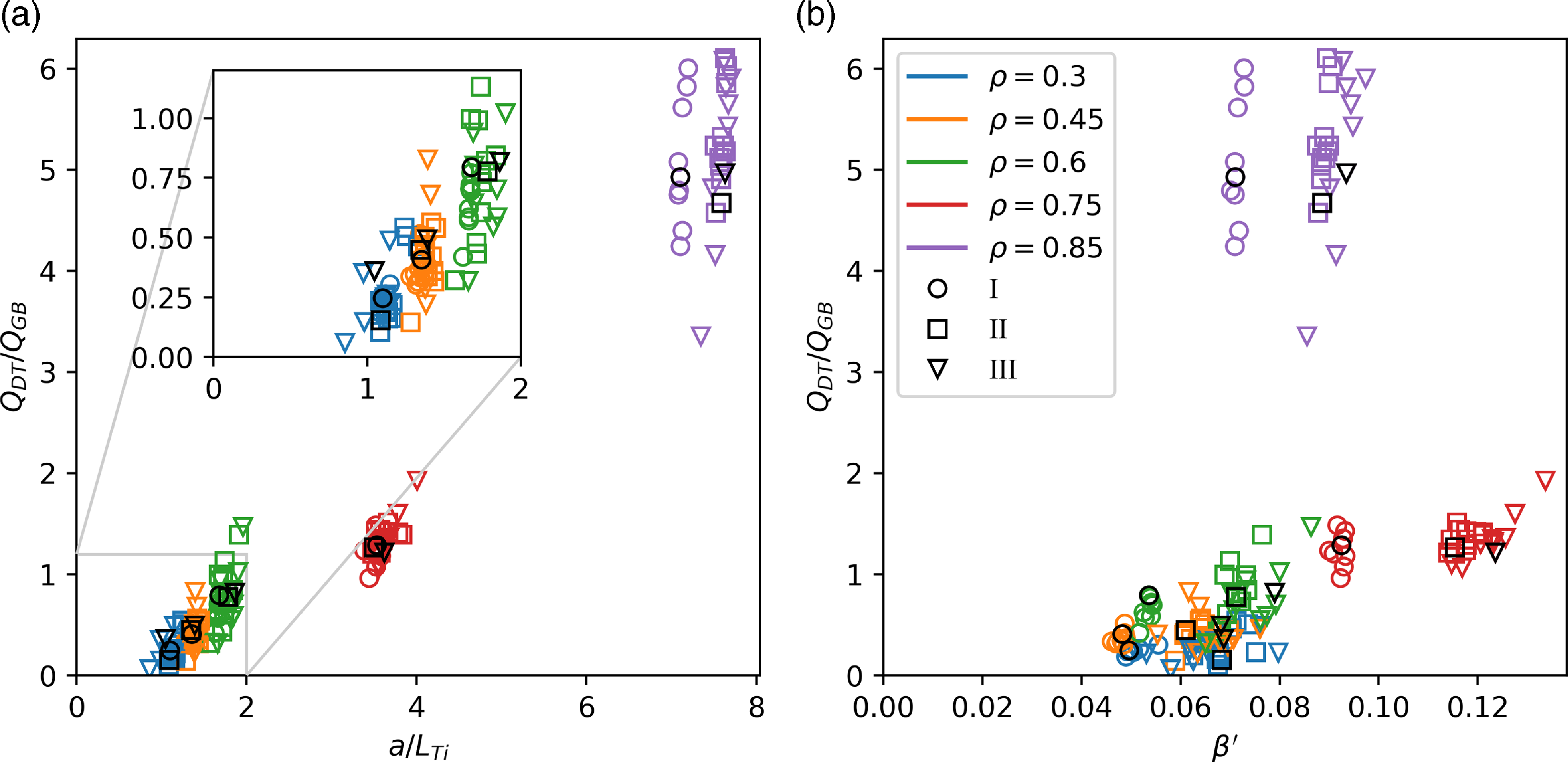
4.4. Impurity transport characteristics
To assess the transport of impurities, additional neoclassical and nonlinear gyrokinetic simulations are run using six kinetic species based on the final predicted profiles for Case I. This enables predicting the particle transport characteristics for electrons, deuterium and tritium fuel ions, helium ash (assumed to be thermal) and neon and tungsten impurities. The same radially constant impurity fractions are used as described in § 4, which means that all particle profiles have flat core density gradient and increasingly large edge density gradient (as in figure 1
a). With these assumptions, the resulting particle flow ( $V' \Gamma _s$
) profiles are shown in figure 13 for each species
$V' \Gamma _s$
) profiles are shown in figure 13 for each species $s$
. As in figure 11, for the fuel ions the integrated source contributions are shown using the pellet fuelling computed from figure 8. For helium ash, the helium ash source rate is shown (dashed red) computed from the deuterium–tritium fusion reaction rate
$s$
. As in figure 11, for the fuel ions the integrated source contributions are shown using the pellet fuelling computed from figure 8. For helium ash, the helium ash source rate is shown (dashed red) computed from the deuterium–tritium fusion reaction rate $\sigma _v$
as
$\sigma _v$
as $S_\alpha = \sigma _v n_D n_T$
, along with the equivalent sink split evenly between the deuterium and tritium species,
$S_\alpha = \sigma _v n_D n_T$
, along with the equivalent sink split evenly between the deuterium and tritium species, $S_{\alpha, D}=S_{\alpha, T}=-0.5 S_\alpha$
. Tungsten and neon are assumed to have no sourcing in this core region. A number of characteristics can be inferred from this analysis.
$S_{\alpha, D}=S_{\alpha, T}=-0.5 S_\alpha$
. Tungsten and neon are assumed to have no sourcing in this core region. A number of characteristics can be inferred from this analysis.
Neoclassical, turbulent and total particle fluxes predicted using final profiles from Case I, but including six kinetic species (deuterium, tritium, e, helium, neon, tungsten) in both SFINCS and GX simulations.
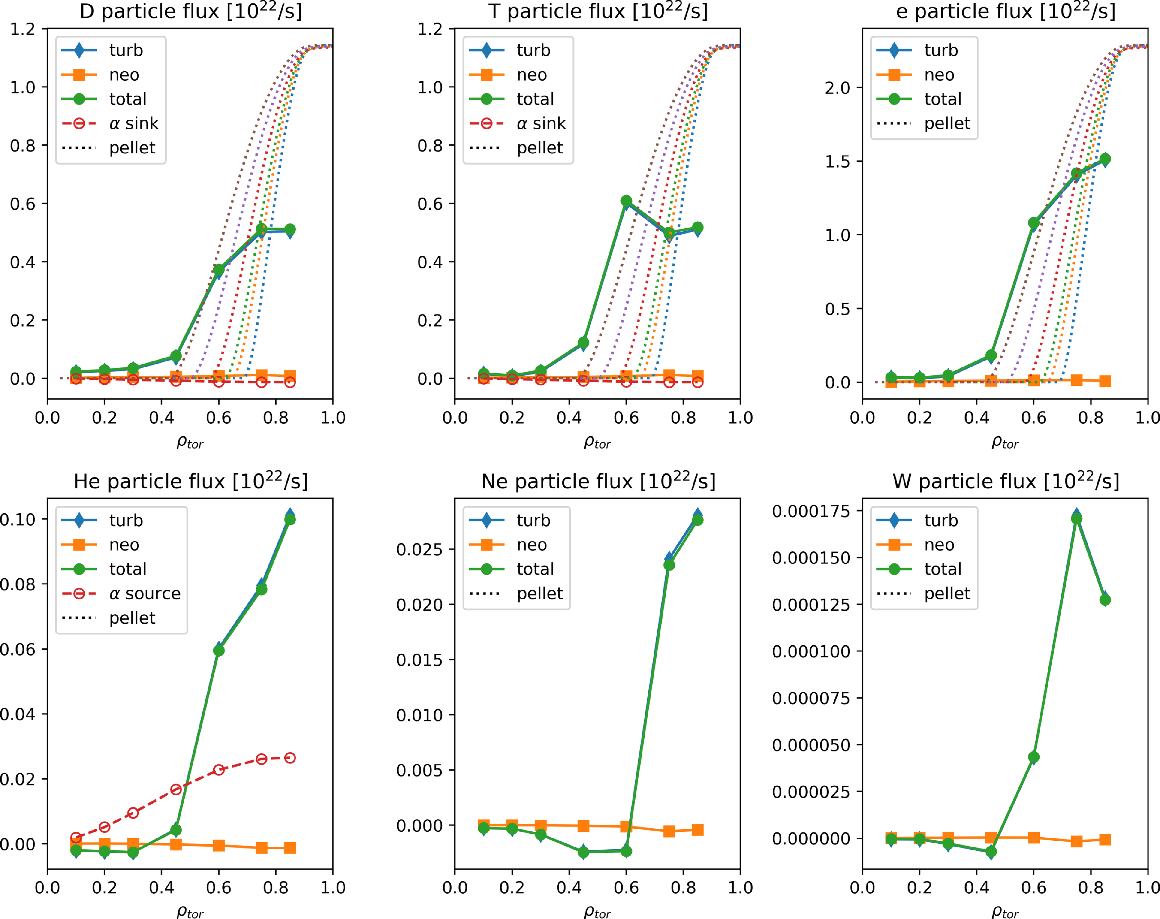
Focusing first on tungsten and neon, the magnitude of turbulent transport is relatively large in the outer region due to the large density gradient there. The tungsten and neon gradients should therefore be smaller in this region for source-free conditions. Deeper in the core where the density gradients flatten, the turbulent impurity fluxes are much smaller and reverse sign to drive an inward pinch. Here, stationary profiles will no longer be flat but instead exhibit some peaking. Over all radii, the magnitudes of turbulent impurity fluxes remain significantly larger than the neoclassical fluxes, $|\Gamma _{s,turb}|/|\Gamma _{s,nc}|\gt 20$
for helium, neon, tungsten (with the exception of tungsten inside
$|\Gamma _{s,turb}|/|\Gamma _{s,nc}|\gt 20$
for helium, neon, tungsten (with the exception of tungsten inside $\rho \leqslant 0.3$
where
$\rho \leqslant 0.3$
where $|\Gamma _{W,turb}|/|\Gamma _{W,nc}|=3\!-\!10$
), regardless of the large variation in assumed density gradients or the variation of turbulence flux transitioning from outward convection to inward pinch. This is true despite the fact that the configuration is in the neoclassical ion root regime (
$|\Gamma _{W,turb}|/|\Gamma _{W,nc}|=3\!-\!10$
), regardless of the large variation in assumed density gradients or the variation of turbulence flux transitioning from outward convection to inward pinch. This is true despite the fact that the configuration is in the neoclassical ion root regime ( $E_r\lt 0$
) (figure 14, computed via SFINCS solving the ambipolar radial electric field as a function of
$E_r\lt 0$
) (figure 14, computed via SFINCS solving the ambipolar radial electric field as a function of $\rho$
), consistent with having very small neoclassical transport in this configuration (
$\rho$
), consistent with having very small neoclassical transport in this configuration ( $\epsilon _{eff}\lt 0.002$
inside
$\epsilon _{eff}\lt 0.002$
inside $\rho \lt 0.7$
; Hegna et al. (Reference Hegna2025)) and dominant ITG turbulence. The implication from these observations is that both neoclassical convection and diffusion are smaller than those from turbulence (
$\rho \lt 0.7$
; Hegna et al. (Reference Hegna2025)) and dominant ITG turbulence. The implication from these observations is that both neoclassical convection and diffusion are smaller than those from turbulence ( $D_{nc}\lt D_{turb}$
,
$D_{nc}\lt D_{turb}$
, $V_{nc}\lt V_{turb}$
), at all radii. Any profile peaking should therefore be determined largely by turbulence. A coarse estimate of peaking is found by determining the density gradient at the radius where
$V_{nc}\lt V_{turb}$
), at all radii. Any profile peaking should therefore be determined largely by turbulence. A coarse estimate of peaking is found by determining the density gradient at the radius where $\Gamma _{s,total}=0$
. From figure 13, linear interpolation gives
$\Gamma _{s,total}=0$
. From figure 13, linear interpolation gives $\Gamma _{s,tot}=0$
between
$\Gamma _{s,tot}=0$
between $\rho =0.4-0.6$
for all impurities, corresponding to
$\rho =0.4-0.6$
for all impurities, corresponding to $a/L_{n,W (\Gamma _W=0)} \leqslant 0.2$
and
$a/L_{n,W (\Gamma _W=0)} \leqslant 0.2$
and $a/L_{n,Ne (\Gamma _{Ne}=0)} \leqslant 0.4$
. These source-free gradient values are very similar to those predicted for W7-X, where gyrokinetic simulations including iron impurities in the trace limit find
$a/L_{n,Ne (\Gamma _{Ne}=0)} \leqslant 0.4$
. These source-free gradient values are very similar to those predicted for W7-X, where gyrokinetic simulations including iron impurities in the trace limit find $a/L_{n,Fe (\Gamma _{Fe}=0)}=0.3-0.6$
over a range of background main ion density gradients (García-Regaña et al. Reference García-Regaña, Barnes, Calvo, González-Jerez, Thienpondt, Sánchez, Parra and St.-Onge2021a). Assuming
$a/L_{n,Fe (\Gamma _{Fe}=0)}=0.3-0.6$
over a range of background main ion density gradients (García-Regaña et al. Reference García-Regaña, Barnes, Calvo, González-Jerez, Thienpondt, Sánchez, Parra and St.-Onge2021a). Assuming $a/L_n=0.6$
represents an upper limit on impurity peaking and is constant at all radii, the resulting ratio of axis to separatrix density would be
$a/L_n=0.6$
represents an upper limit on impurity peaking and is constant at all radii, the resulting ratio of axis to separatrix density would be $n_{w,0}/n_{w,sep} = exp(a/L_n) = 1.8$
. This peaking is smaller than that of the initially assumed profile,
$n_{w,0}/n_{w,sep} = exp(a/L_n) = 1.8$
. This peaking is smaller than that of the initially assumed profile, $n_0/n_{sep}=4$
(§ 3.1), for which dilution and radiation losses have already been accounted in the predictive transport simulations. While the detailed profile shapes will be different, no strong core peaking is expected for this configuration with very low neoclassical transport and ITG dominant transport in the core. Overall core concentration will be largely determined by sourcing and transport in the boundary region. Additional dedicated simulations are required to confirm the profile shapes are consistent with this coarse estimate, and is the subject of ongoing analysis.
$n_0/n_{sep}=4$
(§ 3.1), for which dilution and radiation losses have already been accounted in the predictive transport simulations. While the detailed profile shapes will be different, no strong core peaking is expected for this configuration with very low neoclassical transport and ITG dominant transport in the core. Overall core concentration will be largely determined by sourcing and transport in the boundary region. Additional dedicated simulations are required to confirm the profile shapes are consistent with this coarse estimate, and is the subject of ongoing analysis.
Ambipolar radial electric field, as calculated by SFINCS. The configuration operates in the ion root ( $E_r\lt 0$
).
$E_r\lt 0$
).

The helium fluxes show a similar trend as tungsten and neon, although in this case the profiles must adapt so that turbulent fluxes match the volume-integrated alpha source. The outward flow of helium is greater than this source outside $\rho \gt 0.5$
, indicating the helium fraction will be smaller in the edge in stationary conditions, with peaking in the inner core that is likely to be larger than the tungsten or neon profiles due to the finite source. Self-consistent impurity density profile prediction will be explored in future work, along with investigation of the sourcing and transport of impurities in the periphery that would set the edge boundary values of the impurity species in our transport calculations.
$\rho \gt 0.5$
, indicating the helium fraction will be smaller in the edge in stationary conditions, with peaking in the inner core that is likely to be larger than the tungsten or neon profiles due to the finite source. Self-consistent impurity density profile prediction will be explored in future work, along with investigation of the sourcing and transport of impurities in the periphery that would set the edge boundary values of the impurity species in our transport calculations.
Finally, we note that in comparison with figure 11, the total electron particle flux is reduced $\sim 25\,\%$
at the outer radii, with a small enhancement at the inner radii. The heat fluxes (not shown) behave similarly. It seems likely that the reduction of fluxes in the outer region is consistent with recent simulations showing that large impurity density gradients can stabilize ITG dynamics (García-Regaña et al. Reference García-Regaña, Calvo, Parra and Thienpondt2024). However, if the impurity density gradients in the edge flatten, as expected, the turbulence suppression effect would be weaker than shown here.
$\sim 25\,\%$
at the outer radii, with a small enhancement at the inner radii. The heat fluxes (not shown) behave similarly. It seems likely that the reduction of fluxes in the outer region is consistent with recent simulations showing that large impurity density gradients can stabilize ITG dynamics (García-Regaña et al. Reference García-Regaña, Calvo, Parra and Thienpondt2024). However, if the impurity density gradients in the edge flatten, as expected, the turbulence suppression effect would be weaker than shown here.
5. Operational considerations
Plasma operating contour (POPCON) analysis is performed to evaluate operational and scenario development considerations, shown in figure 15. The analysis is performed by scaling the density and temperature profiles predicted in Case III (see figure 9) while constraining volume-averaged power balance with the corresponding confinement quality $f_c=1.14$
relative to the ISS04 scaling. This amounts to solving for the integrated auxiliary power required to balance the integrated transport and radiative losses via
$f_c=1.14$
relative to the ISS04 scaling. This amounts to solving for the integrated auxiliary power required to balance the integrated transport and radiative losses via $P_{{heat}} = P_{{loss}}$
, with
$P_{{heat}} = P_{{loss}}$
, with $P_{{heat}} = P_{{aux}} + P_\alpha$
, and
$P_{{heat}} = P_{{aux}} + P_\alpha$
, and
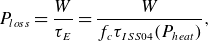 \begin{equation} P_{{loss}} = \frac {W}{\tau _E} = \frac {W}{f_c \tau _{ISS04}(P_{{heat}})}, \end{equation}
where $P_{{loss}}$
includes radiative losses, consistent with the definitions of
$P_{{loss}}$
includes radiative losses, consistent with the definitions of $\tau _E$
and
$\tau _E$
and $f_c$
specified in § 4. This can be solved for
$f_c$
specified in § 4. This can be solved for $P_{{aux}}$
as
$P_{{aux}}$
as
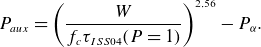 \begin{equation} P_{{aux}} = \left (\frac {W}{f_c \tau _{ISS04}(P=1)}\right )^{2.56} - P_\alpha . \end{equation}
POPCON analysis using the density and temperature profile shapes from case II, scaled by constant factors to vary $\langle n_e \rangle$
and
$\langle n_e \rangle$
and $\langle T_e \rangle$
, and the corresponding confinement quality
$\langle T_e \rangle$
, and the corresponding confinement quality $f_c=1.14$
. Stars indicate T3D cases I (blue), II (orange) and III (green).
$f_c=1.14$
. Stars indicate T3D cases I (blue), II (orange) and III (green).
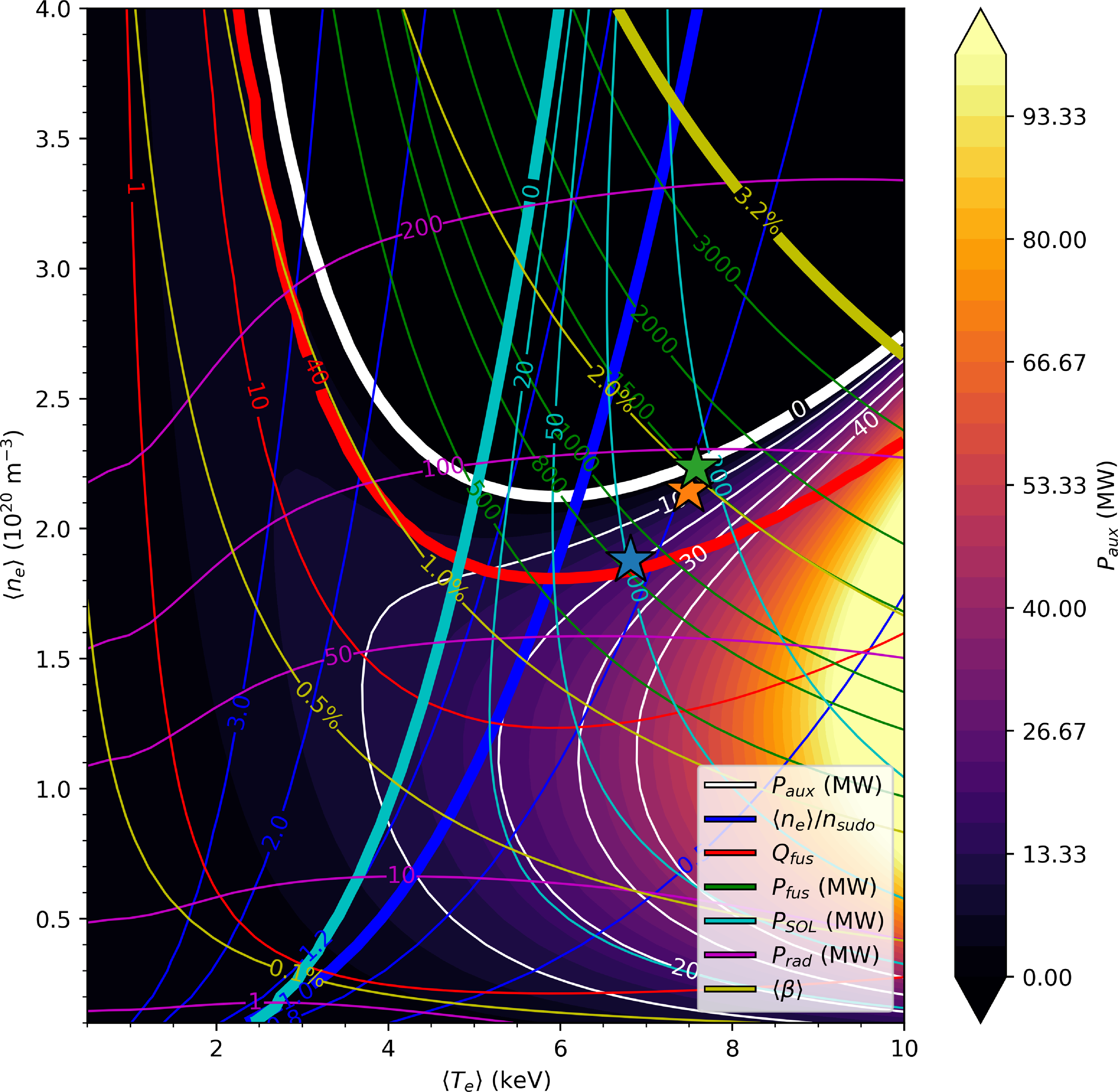
The profiles are interpolated to a finer radial grid ( $N_r=100$
), and we assume an exponential drop of the temperature from
$N_r=100$
), and we assume an exponential drop of the temperature from $T(\rho =0.9)=2$
keV to
$T(\rho =0.9)=2$
keV to $T(\rho =1)=0.1$
keV. The volume-averaged electron density and electron temperature of the scaled profiles are shown in the horizontal and vertical axes. Contours of auxiliary power (
$T(\rho =1)=0.1$
keV. The volume-averaged electron density and electron temperature of the scaled profiles are shown in the horizontal and vertical axes. Contours of auxiliary power ( $P_{{aux}}$
), Sudo density fraction (
$P_{{aux}}$
), Sudo density fraction ( $f_{{Sudo}}=\langle n_e \rangle /n_{{Sudo}}$
), fusion gain (
$f_{{Sudo}}=\langle n_e \rangle /n_{{Sudo}}$
), fusion gain ( $Q_{{fus}}$
), exhaust power (
$Q_{{fus}}$
), exhaust power ( $P_{{SOL}}$
), radiated power (
$P_{{SOL}}$
), radiated power ( $P_{{rad}}$
) and volume-averaged beta (
$P_{{rad}}$
) and volume-averaged beta ( $\langle \beta \rangle$
) are shown with various colours. Key operational boundaries are highlighted with thick lines: the
$\langle \beta \rangle$
) are shown with various colours. Key operational boundaries are highlighted with thick lines: the $\langle \beta \rangle = 3.2\,\%$
contour, representing the global MHD stability limit; the
$\langle \beta \rangle = 3.2\,\%$
contour, representing the global MHD stability limit; the $Q_{{fus}}=40$
contour, representing desired fusion gain for operation; the
$Q_{{fus}}=40$
contour, representing desired fusion gain for operation; the $P_{{aux}}=0$
contour, representing ignition (
$P_{{aux}}=0$
contour, representing ignition ( $Q_{{fus}}=\infty$
); the
$Q_{{fus}}=\infty$
); the $P_{{SOL}}=0$
contour, which represents the boundary of radiative collapse; and the
$P_{{SOL}}=0$
contour, which represents the boundary of radiative collapse; and the $\langle n_e \rangle /n_{{Sudo}}=1$
contour, which is another metric of radiative limits. This shows that a wide region of stable high gain is accessible.
$\langle n_e \rangle /n_{{Sudo}}=1$
contour, which is another metric of radiative limits. This shows that a wide region of stable high gain is accessible.
The stars denote the operating points for the three cases discussed in § 4. Case I (blue star) lies at the intersection of the bold red $Q_{{fus}}=40$
contour and the green
$Q_{{fus}}=40$
contour and the green $P_{{fus}}=800$
MW contour, between the
$P_{{fus}}=800$
MW contour, between the $\langle n_e \rangle /n_{{Sudo}} = 0.8$
and
$\langle n_e \rangle /n_{{Sudo}} = 0.8$
and $\langle n_e \rangle /n_{{Sudo}} = 1$
blue contours. The operating point for Case II (orange star) appears to lie on the
$\langle n_e \rangle /n_{{Sudo}} = 1$
blue contours. The operating point for Case II (orange star) appears to lie on the $P_{{aux}}=10$
MW contour, despite the fact that this case used 20 MW of auxiliary heating power; this discrepancy can be explained by the fact that Case II has a slightly lower
$P_{{aux}}=10$
MW contour, despite the fact that this case used 20 MW of auxiliary heating power; this discrepancy can be explained by the fact that Case II has a slightly lower $f_c = 1.13$
, which would tend to shift the
$f_c = 1.13$
, which would tend to shift the $P_{{aux}}$
curves slightly. Case III (green star) lies on the
$P_{{aux}}$
curves slightly. Case III (green star) lies on the $P_{{aux}}=0$
contour on the edge of the ignition region, as expected.
$P_{{aux}}=0$
contour on the edge of the ignition region, as expected.
The POPCON also indicates that operation with $Q\gt 40$
with lower exhaust power due to substantial radiated power is possible in the region between the
$Q\gt 40$
with lower exhaust power due to substantial radiated power is possible in the region between the $\langle n_e \rangle /n_{{Sudo}} = 1$
thick blue contour and the
$\langle n_e \rangle /n_{{Sudo}} = 1$
thick blue contour and the $P_{SOL}=0$
thick cyan contour. However, the viability of this potential operating region assumes that confinement quality will remain the same at lower temperature. We also are not currently accounting for additional radiation in the outer 10 % of the volume, where we expect to operate with a radiative mantle via injected low-Z impurities. This could enable lower exhaust power at temperatures closer to the operating points considered here.
$P_{SOL}=0$
thick cyan contour. However, the viability of this potential operating region assumes that confinement quality will remain the same at lower temperature. We also are not currently accounting for additional radiation in the outer 10 % of the volume, where we expect to operate with a radiative mantle via injected low-Z impurities. This could enable lower exhaust power at temperatures closer to the operating points considered here.
While operating at or close to ignition is favourable for reducing stationary recirculating power, a minimum amount of auxiliary power will be required at start-up to access the operating point. To more clearly illustrate this, figure 16 shows various parameters evaluated along curves of constant $f_{{Sudo}}=\langle n_e\rangle / n_{{Sudo}}$
as volume-averaged density is increased. Squares show where each curve intersects the
$f_{{Sudo}}=\langle n_e\rangle / n_{{Sudo}}$
as volume-averaged density is increased. Squares show where each curve intersects the $P_{{fus}}=800$
MW contour (same as Case I), while circles show the intersection with the
$P_{{fus}}=800$
MW contour (same as Case I), while circles show the intersection with the $P_{{fus}}=1.3$
GW contour (same as Case II). Figure 16(c) shows that less than 25 MW of auxiliary power is required to reach the operating points via the
$P_{{fus}}=1.3$
GW contour (same as Case II). Figure 16(c) shows that less than 25 MW of auxiliary power is required to reach the operating points via the $f_{{Sudo}}=1$
curve, and less than 20 MW is required along the
$f_{{Sudo}}=1$
curve, and less than 20 MW is required along the $f_{{Sudo}}=1.2$
curve. Increasing the Sudo fraction at constant
$f_{{Sudo}}=1.2$
curve. Increasing the Sudo fraction at constant $P_{{fus}}$
increases the radiated power and thus lowers the amount of power conducted into the periphery, dropping
$P_{{fus}}$
increases the radiated power and thus lowers the amount of power conducted into the periphery, dropping $P_{{SOL}} \leqslant$
20 MW for the 800 MW operating point at
$P_{{SOL}} \leqslant$
20 MW for the 800 MW operating point at $f_{{Sudo}}= 1.2$
. Also note that the
$f_{{Sudo}}= 1.2$
. Also note that the $P_{{rad}}$
contours on the POPCON are approximately orthogonal to the
$P_{{rad}}$
contours on the POPCON are approximately orthogonal to the $f_{{Sudo}}$
contours, which results in the
$f_{{Sudo}}$
contours, which results in the $P_{{rad}}$
curves overlapping for different values of
$P_{{rad}}$
curves overlapping for different values of $f_{{Sudo}}$
in figure 16(f). All three curves maintain net positive power flow (
$f_{{Sudo}}$
in figure 16(f). All three curves maintain net positive power flow ( $P_{{SOL}}\gt 0$
), indicating that the plasma remains below the true radiative density limit even as radiated power increases with density.
$P_{{SOL}}\gt 0$
), indicating that the plasma remains below the true radiative density limit even as radiated power increases with density.
Various quantities computed along curves of constant $f_{{Sudo}}=\langle n_e\rangle /n_{{Sudo}}$
in the POPCON. Squares show where each curve intersects with
$f_{{Sudo}}=\langle n_e\rangle /n_{{Sudo}}$
in the POPCON. Squares show where each curve intersects with $P_{{fus}}=800$
MW contour (same as Case I); circles show where each curve intersects the
$P_{{fus}}=800$
MW contour (same as Case I); circles show where each curve intersects the $P_{{fus}}=1.3$
GW contour (same as Case II).
$P_{{fus}}=1.3$
GW contour (same as Case II).
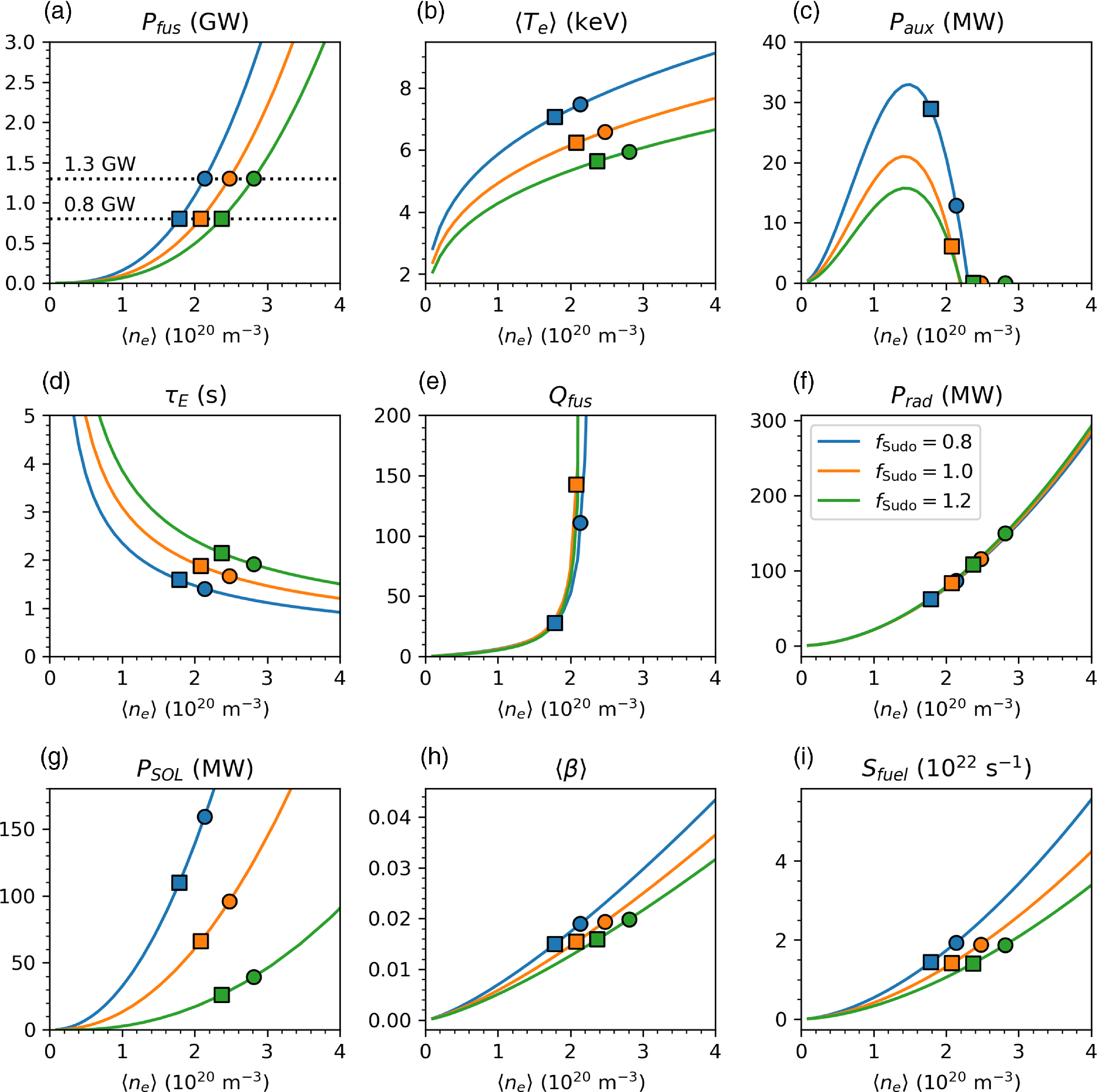
The pellet fuelling required to access the operating point along constant Sudo fraction can be estimated by assuming the ratio of particle to energy confinement time is constant. For Case I, the particle confinement time can be estimated as $\tau _p = \langle n_e \rangle V / \Gamma _e(\rho =1) \approx 4$
s, so that
$\tau _p = \langle n_e \rangle V / \Gamma _e(\rho =1) \approx 4$
s, so that $\tau _p/\tau _E \approx 3$
. The fuelling rate along the constant Sudo fraction curves is then computed as
$\tau _p/\tau _E \approx 3$
. The fuelling rate along the constant Sudo fraction curves is then computed as $S_{{fuel}} = \langle n_e \rangle V / (3 \tau _E)$
. Assuming constant confinement quality, figure 16(i) shows that the maximum requirement for fuelling will occur at the operating point. Potential degradation of confinement quality in the lower density start-up regime (perhaps due to
$S_{{fuel}} = \langle n_e \rangle V / (3 \tau _E)$
. Assuming constant confinement quality, figure 16(i) shows that the maximum requirement for fuelling will occur at the operating point. Potential degradation of confinement quality in the lower density start-up regime (perhaps due to $T_e/T_i\gt 1$
) could be mitigated by deeper pellet penetration at lower temperatures.
$T_e/T_i\gt 1$
) could be mitigated by deeper pellet penetration at lower temperatures.
Going to higher $f_{{Sudo}}$
also moves the operating point towards the thermally unstable side of the ignition curve, which would require a burn control strategy to maintain stationary operation. Figure 16(d) shows that as fusion power increases the energy confinement time falls, which is expected as
$f_{{Sudo}}$
also moves the operating point towards the thermally unstable side of the ignition curve, which would require a burn control strategy to maintain stationary operation. Figure 16(d) shows that as fusion power increases the energy confinement time falls, which is expected as $\tau _E\sim (n/P_{{fus}})^{3/5}$
with
$\tau _E\sim (n/P_{{fus}})^{3/5}$
with $P_{{fus}}\sim n^2$
increasing faster than the density. Again assuming the ratio of particle to energy confinement time is approximately constant, fixed core fuelling will no longer sustain the density or edge density gradient, such that both fusion power and energy confinement quality will be degraded. Furthermore, pellet deposition will become increasingly shallower as temperatures increase, further reducing energy confinement. This should provide a natural throttling mechanism to thermal instability. Soft beta limits due to ballooning modes (kinetic and/or ideal) may also have a similar effect depending on the proximity to the stability margin (Zhou et al. Reference Zhou, Aleynikova, Liu and Ferraro2024). Additional control techniques like varying isotope mix also remain a viable burn control strategy.
$P_{{fus}}\sim n^2$
increasing faster than the density. Again assuming the ratio of particle to energy confinement time is approximately constant, fixed core fuelling will no longer sustain the density or edge density gradient, such that both fusion power and energy confinement quality will be degraded. Furthermore, pellet deposition will become increasingly shallower as temperatures increase, further reducing energy confinement. This should provide a natural throttling mechanism to thermal instability. Soft beta limits due to ballooning modes (kinetic and/or ideal) may also have a similar effect depending on the proximity to the stability margin (Zhou et al. Reference Zhou, Aleynikova, Liu and Ferraro2024). Additional control techniques like varying isotope mix also remain a viable burn control strategy.
6. Discussion and summary
Transport characteristics and predicted confinement and performance are shown for the Infinity Two fusion pilot plant baseline plasma physics design, a high field stellarator concept developed using modern optimization techniques. Analysis using nonlinear EM gyrokinetics (i.e. GX) confirms that a scenario with large density gradient substantially reduces ITG-dominant transport. The maintained suppression of transport at increasing density gradient confirms that deleterious TEM dynamics have been minimized, consistent with the maximum-J condition being satisfied in this QI configuration. The stability boundary for KBM onset is shown to be similar to the ideal ballooning mode limit, and occurs at beta values $\sim 50 \,\%$
above the desired operating point in the region of large gradients. Electromagnetic effects do, however, provide additional reduction of turbulent transport at increasing
$\sim 50 \,\%$
above the desired operating point in the region of large gradients. Electromagnetic effects do, however, provide additional reduction of turbulent transport at increasing $\beta$
. In this regime, the electron thermal transport is larger than ion thermal transport, due in part to growing contributions from magnetic flutter at wavenumbers
$\beta$
. In this regime, the electron thermal transport is larger than ion thermal transport, due in part to growing contributions from magnetic flutter at wavenumbers $k_y\rho _i \sim 1$
, which may be associated with linearly unstable tearing parity modes that are highly elongated along magnetic field lines. Such distinctive conditions may be present in future W7-X high-beta operations, which offers a potential test bed to validate related predictions in similar operational scenarios.
$k_y\rho _i \sim 1$
, which may be associated with linearly unstable tearing parity modes that are highly elongated along magnetic field lines. Such distinctive conditions may be present in future W7-X high-beta operations, which offers a potential test bed to validate related predictions in similar operational scenarios.
High-fidelity predictions of temperature profiles and global performance have been made using the T3D transport solver, coupled with the gyrokinetic turbulence simulations (i.e. GX) and drift kinetic neoclassical simulations (i.e. SFINCS). Converged transport solutions are shown for a baseline operating point ( $P_{{fus,DT}}$
= 800 MW,
$P_{{fus,DT}}$
= 800 MW, $Q_{{fus}}=40$
,
$Q_{{fus}}=40$
, $\langle n \rangle = 1.88 \times 10^{20}$
m
$\langle n \rangle = 1.88 \times 10^{20}$
m $^{-3}$
) and higher power (
$^{-3}$
) and higher power ( $P_{{fus,DT}}$
= 1.3–1.5 GW) operating points, including an ignited scenario (
$P_{{fus,DT}}$
= 1.3–1.5 GW) operating points, including an ignited scenario ( $Q_{{fus}}= \infty$
). All cases correspond to
$Q_{{fus}}= \infty$
). All cases correspond to $f_{{Sudo}}=\langle n_e\rangle /n_{{Sudo}} \lt 1$
and
$f_{{Sudo}}=\langle n_e\rangle /n_{{Sudo}} \lt 1$
and $\langle \beta \rangle = 1.5-1.9\,\%$
, below the global stability limit (3.2 %) as desired for conservative operation within known stability boundaries. Analysis confirms that neoclassical energy transport is negligible compared with turbulence, as expected with the small
$\langle \beta \rangle = 1.5-1.9\,\%$
, below the global stability limit (3.2 %) as desired for conservative operation within known stability boundaries. Analysis confirms that neoclassical energy transport is negligible compared with turbulence, as expected with the small $\epsilon _{{eff}}$
values for this device. The traditionally defined energy confinement quality factors
$\epsilon _{{eff}}$
values for this device. The traditionally defined energy confinement quality factors $f_c = \tau _E / \tau _{{ISS04}}= 1.12-1.14$
are somewhat lower than desired. However, these cases have large core radiation fraction (
$f_c = \tau _E / \tau _{{ISS04}}= 1.12-1.14$
are somewhat lower than desired. However, these cases have large core radiation fraction ( $f_{\mathrm {rad}}=35-40\,\%$
) due to the assumed impurities (helium, neon and tungsten, with constant
$f_{\mathrm {rad}}=35-40\,\%$
) due to the assumed impurities (helium, neon and tungsten, with constant $Z_{{eff}}=1.62$
). Subtracting the large radiated power from the net heating power, the larger ‘conduction-only’ confinement quality
$Z_{{eff}}=1.62$
). Subtracting the large radiated power from the net heating power, the larger ‘conduction-only’ confinement quality $f_{c,cond}=1.33-1.41$
is representative of the confinement characteristics expected in conditions with much lower radiation. The predicted particle fluxes are roughly consistent with fuelling profiles from pellet ablation calculations based on W7-X injector technology assuming slightly larger ITER-sized pellets, confirming the desired fuel ion profile shapes are plausible. Impurity transport from multispecies calculations using the same constant concentrations as used in the T3D cases indicate large outward impurity particle fluxes are expected in the outer-half radius, favourable for avoiding core accumulation of the source-free impurities. While neoclassical particle fluxes remain smaller than turbulent fluxes deep into the high temperature core (
$f_{c,cond}=1.33-1.41$
is representative of the confinement characteristics expected in conditions with much lower radiation. The predicted particle fluxes are roughly consistent with fuelling profiles from pellet ablation calculations based on W7-X injector technology assuming slightly larger ITER-sized pellets, confirming the desired fuel ion profile shapes are plausible. Impurity transport from multispecies calculations using the same constant concentrations as used in the T3D cases indicate large outward impurity particle fluxes are expected in the outer-half radius, favourable for avoiding core accumulation of the source-free impurities. While neoclassical particle fluxes remain smaller than turbulent fluxes deep into the high temperature core ( $\rho =0.1$
), the turbulence itself provides an impurity pinch. It is estimated that the resulting peaking is actually smaller than that assumed in the predictive transport simulations. Self-consistent predictions of fuel, helium ash and impurity density profiles will require additional simulations to quantify the range of expected concentrations and peaking factors. Finally, POPCON analysis using the predicted profile shapes and confinement quality indicates a wide range of high gain operating space is available. In particular, even higher core radiation fraction and lower
$\rho =0.1$
), the turbulence itself provides an impurity pinch. It is estimated that the resulting peaking is actually smaller than that assumed in the predictive transport simulations. Self-consistent predictions of fuel, helium ash and impurity density profiles will require additional simulations to quantify the range of expected concentrations and peaking factors. Finally, POPCON analysis using the predicted profile shapes and confinement quality indicates a wide range of high gain operating space is available. In particular, even higher core radiation fraction and lower $P_{\mathrm {SOL}}$
are accessible while retaining high gain, assuming stable operation at slightly elevated Sudo fraction (
$P_{\mathrm {SOL}}$
are accessible while retaining high gain, assuming stable operation at slightly elevated Sudo fraction ( $f_{{Sudo}} \leqslant$
1.2). Additional analysis is required to predict the trade-off between core versus edge mantle radiation and corresponding impact on performance characteristics.
$f_{{Sudo}} \leqslant$
1.2). Additional analysis is required to predict the trade-off between core versus edge mantle radiation and corresponding impact on performance characteristics.
While our results are favourable for the operation of the Infinity Two pilot plant, there remain a number of assumptions and uncertainties that can impact performance, all of which will be the subject of future work. A number of the assumptions we have made in the transport calculations are likely conservative: we have assumed 10 % alpha heating losses, which from ASCOT calculations in Carbajal et al. (Reference Carbajal2025) may be less than 5 %; we have assumed a 5 % helium ash concentration, which may be reduced with the favourable outward particle fluxes observed in excess of the $\alpha$
source rate; we have not included effects of turbulence suppression induced by impurity dilution; and we have not included the effects of the radial electric field in the turbulence calculations, which can also suppress turbulence, particularly near the edge (Wilms et al. Reference Wilms2024). On the other hand, the assumptions we have made about the density profile shape and the edge temperature may prove to be overly optimistic. While continuing work will address self-consistent density prediction within our transport calculations, the ability to quantitatively predict plasma parameters near the separatrix and out into the open field line region with islands and divertor is much less mature than for core plasma physics. All of these uncertainties, in part, motivate the construction and operation of the new Infinity One stellarator facility currently being designed by Type One Energy, with nominal parameters
$\alpha$
source rate; we have not included effects of turbulence suppression induced by impurity dilution; and we have not included the effects of the radial electric field in the turbulence calculations, which can also suppress turbulence, particularly near the edge (Wilms et al. Reference Wilms2024). On the other hand, the assumptions we have made about the density profile shape and the edge temperature may prove to be overly optimistic. While continuing work will address self-consistent density prediction within our transport calculations, the ability to quantitatively predict plasma parameters near the separatrix and out into the open field line region with islands and divertor is much less mature than for core plasma physics. All of these uncertainties, in part, motivate the construction and operation of the new Infinity One stellarator facility currently being designed by Type One Energy, with nominal parameters $R \sim 3$
m and
$R \sim 3$
m and $B \sim 3$
T. The primary physics objectives for Infinity One include demonstrating and validating the ability to improve turbulent transport while also establishing a compatible divertor concept that provides scalable solutions for managing power and particle exhaust.
$B \sim 3$
T. The primary physics objectives for Infinity One include demonstrating and validating the ability to improve turbulent transport while also establishing a compatible divertor concept that provides scalable solutions for managing power and particle exhaust.
Acknowledgements
This work was supported by Type One Energy. We gratefully acknowledge our use of computing resources and facilities funded by the U.S. Department of Energy, including: the Oak Ridge Leadership Computing Facility at the Oak Ridge National Laboratory, which is supported by the Office of Science of the U.S. Department of Energy under contract no. DE-AC 05–00OR22725, using awards for computing time on Summit and Frontier; the National Energy Research Scientific Computing Center (NERSC), a Department of Energy Office of Science User Facility, using NERSC awards FES-ERCAP27470 and FES-ERCAP0031820 for computing time on Perlmutter; the Argonne Leadership Computing Facility, a U.S. DOE Office of Science user facility at Argonne National Laboratory, which is supported by the Office of Science of the U.S. DOE under contract no. DE-AC 02–06CH11357, using an award for computing time on Polaris provided by the U.S. Department of Energy’s (DOE) Innovative and Novel Computational Impact on Theory and Experiment (INCITE) Program. We also gratefully acknowledge the use of computational resources managed and supported by Princeton Research Computing, a consortium of groups including the Princeton Institute for Computational Science and Engineering (PICSciE) and the Office of Information Technology’s High Performance Computing Center and Visualization Laboratory at Princeton University.
Editor Per Helander thanks the referees for their advice in evaluating this article.
Declaration of interests
The work of W.D.D. and M.L. was performed as consultants and was not part of the employees’ responsibilities to the University of Maryland. The work of C.H. was performed as a consultant and was not part of the employee’s responsibilities to the University of California – San Diego.


 Open access