2. Problem set-up and numerical methods

In this section, we first introduce the problem set-up and governing equations in § 2.1. Then, in § 2.2, we describe the numerical methods employed to simulate the air and water flows and track the dynamic air–water interface. Finally, we present the computational parameters in § 2.3.

2.1. Problem set-up and governing equations

In our mechanistic study of ventilated cavitation and the turbulent flow therein, we consider a computational setting with a ventilating cavitator located inside a rectangular water tunnel with uniform water inflow from the inlet. In the present simulation, we consider only the case in which the mainstream velocity is not very high so that the natural cavitation regime is not attained. In other words, the influence of natural cavitation effects on the cavity is not considered in our computational setting. Figure 1(a) shows the computational domain in our coordinate system, with $x$, $y$ and $z$ denoting the streamwise, vertical and transverse directions, respectively. The water flows through the inlet with velocity $U_\infty$ in the $x$ direction, passes the cavity, and exits through the outlet. In the simulation, a Dirichlet boundary condition is imposed at the inlet, and a convective boundary condition is applied at the outlet (Lodato, Domingo & Vervisch Reference Lodato, Domingo and Vervisch2008).

Figure 1.

Schematic of the simulation set-up: (a) computational domain, and (b) cavity, cavitator and ventilation source. The blue arrow on the left of the cavitator indicates the water inflow direction. The green arrows indicate the air ventilation directions.

Figure 1(b) shows a schematic of the cavity, with the cavitator and ventilation source indicated. The cavitator, which is located on the central axis at $x_{c}=30d_{c}$, is a circular disk with diameter $d_{c}$ and thickness $0.3d_{c}$. We use a spherical source region with diameter $0.6d_{c}$ that is located $1d_{c}$ behind the disk to generate ventilation in the simulation. This numerical treatment overcomes the numerical difficulty of representing a practical small air ventilation configuration with limited grid resolution. More numerical details are provided in § 2.2. In our experiments and applications, air is ventilated out through a vent port mounted on the strut, which is used to support the cavitator. The shape and position of the vent port and the air ventilation direction can influence the cavity (Semenenko Reference Semenenko2001). Because the aim of the present work is to elucidate the fundamental mechanisms of the cavity, the complex object and vent settings can be replaced by a simplified model without loss of generality in this mechanistic study.

In the simulation, a fluid system with variational densities and viscosities is used to treat the air and water simultaneously. The fluid motion is governed by the incompressible Navier–Stokes equations and continuity equation as follows:

(2.1)$$\begin{gather} \frac{\partial u_{i}}{\partial t}+\frac{\partial(u_{i}u_{j})}{\partial x_{j}}={-}\frac{1}{\rho}\,\frac{\partial p}{\partial x_{i}} + g_{i} + \frac{1}{\rho}\,\frac{\partial\sigma_{ij}}{\partial x_{j}} + \frac{1}{\rho}\,T_{i}, \end{gather}$$

(2.2)$$\begin{gather}\frac{\partial u_{j}}{\partial x_{j}}=0. \end{gather}$$

In the above equations, $x_{i}$ ($i = 1, 2, 3$) denote the Cartesian coordinates $(x, y, z)$, $u_i$ are the $(u, v, w)$ components of the flow velocity, $\rho$ is the density of the fluid, $p$ is the dynamic pressure, $g_i$ ($i = 1, 2, 3$) indicate the components of the gravitational acceleration, $\sigma _{ij}=\mu (\partial u_i/\partial x_j+\partial u_j/\partial x_i)$ ($i, j = 1, 2, 3$) denote the components of the stress tensor, $T_{i}$ ($i = 1, 2, 3$) denote the components of the surface tension at the air–water interface, and $\mu$ is the dynamic viscosity.

2.2. Numerical methods

The momentum equations (2.1) are spatially discretized using the second-order central difference scheme. Several considerations were noted when we adopted this scheme. First, this scheme is simple to implement and requires less computational time per step than other approaches. Furthermore, this scheme works robustly with our approach for solving the Poisson equation. Moreover, the short stencil of this scheme allows us to implement the immersed boundary method and the coupled level set and volume-of-fluid (CLSVOF) method, and increases the numerical robustness. Finally, this scheme is numerically non-dissipative, which enables the DNS to resolve turbulent motions over a wide range of scales. The second-order Runge–Kutta (RK2) method is employed for time advancement. To enforce the continuity equation (2.2), the fractional-step method (Kim & Moin Reference Kim and Moin1985) is utilized at each substep of the RK2 method. The pressure is obtained by solving the Poisson equation as follows:

(2.3)\begin{equation} \frac{\partial}{\partial x_{i}}\left(\frac{1}{\rho}\,\frac{\partial p}{\partial x_{i}}\right)=\frac{1}{{\rm \Delta} t} \left(\frac{\partial u_{j}^{*}}{\partial x_{j}} - S\varPhi \right), \end{equation}

where ${\rm \Delta} t$ is the time step, and $u^{*}$ is the intermediate velocity in the projection method without adding the pressure gradient in (2.1). Moreover,

(2.4)\begin{equation} S=\frac{u_{0}4{\rm \pi} (0.5d_{s})^2}{\frac{4}{3}{\rm \pi} (0.5d_{s})^{3}}=\frac{10u_{0}}{d_{c}}\end{equation}

is the divergence constant in the ventilation source, $\varPhi$ is a Heaviside function that equals 1 inside the ventilation source and 0 otherwise, $d_{s}=0.6d_{c}$ is the diameter of the ventilation source, and $u_{0}$ is the uniform air ventilation speed (sketched in figure 1a). The uniform air ventilation speed $u_{0}$ can be calculated using the air entrainment coefficient $C_{q}=Q/(U_{\infty }d_{c}^2)$, where $Q$ is the air ventilation rate:

(2.5)\begin{equation} u_{0} = \frac{C_{q}(U_{\infty}d_{c}^{2})}{4{\rm \pi}(0.5d_{s})^2} =\frac{25C_{q}U_{\infty}}{9{\rm \pi}}.\end{equation}

Equation (2.3) is a Poisson equation with a large matrix because it involves grid points in three dimensions. The direct inversion of such a large matrix is computationally prohibitive. As a result, this matrix needs to be solved with an iterative method. Moreover, the simulations must be performed on large parallel computers, which increases the computational costs. The portable extensible toolkit for scientific computation (PETSc) package has been applied in many previous studies (see e.g. Balay et al. Reference Balay, Abhyankar, Adams, Brown, Brune, Buschelman, Dalcin, Eijkhout, Gropp and Kaushik2017; Yang, Deng & Shen Reference Yang, Deng and Shen2018; Gao, Deane & Shen Reference Gao, Deane and Shen2021b) and has been shown to be computationally efficient and robust in solving the Poisson equation. Thus this package is adopted in this study.

The air–water interface is captured using the CLSVOF method (Sussman & Puckett Reference Sussman and Puckett2000). The level set function $\psi$ describes the distance to the air–water interface, with positive and negative values in the water and air, respectively. The zero value of $\psi$ corresponds to the interface. The norm of the gradient of $\psi$ is identically unity, i.e.

(2.6)\begin{equation} |\boldsymbol{\nabla}\psi|=1.\end{equation}

The governing equation of $\psi$ takes the form

(2.7)\begin{equation} \frac{\partial \psi}{\partial t} + u_{j}\,\frac{\partial\psi}{\partial x_{j}}=0,\end{equation}

which can be spatially discretized by applying a second-order essential non-oscillatory scheme (Shu & Osher Reference Shu and Osher1989), and integrated over time with a second-order operator-splitting method. A reinitialization procedure (Min Reference Min2010) is employed to ensure that the advected $\psi$ is the signed-distance function described by (2.6).

The air and water phases are recognized by their density and viscosity, which are determined based on the level set function $\psi$ as

(2.8)$$\begin{gather} \rho=H(\psi)\,\rho_{w} + (1-H(\psi))\,\rho_{a}, \end{gather}$$

(2.9)$$\begin{gather}\mu=H(\psi)\,\mu_{w} + (1-H(\psi))\,\mu_{a}, \end{gather}$$

where $H(\psi )$ is the Heaviside function, $\rho _{w}$ and $\rho _{a}$ are the densities of water and air, and $\mu _{w}$ and $\mu _{a}$ are the dynamic viscosities of water and air, respectively. In the simulation, these values are smoothed near the air–water interface as

(2.10)\begin{equation} H(\psi)= \left\{\begin{array}{@{}ll@{}} 0, & \psi<{-}\epsilon,\\ \displaystyle \dfrac{1}{2}\left[1+\dfrac{\psi}{\epsilon}+\dfrac{1}{\rm \pi} \sin\left(\dfrac{\psi{\rm \pi}}{\epsilon}\right)\right], & |\psi|\leq\epsilon,\\ 1, & \psi>\epsilon. \end{array}\right. \end{equation}

Here, $\epsilon$ is the half-thickness of the diffusion region. According to our previous research (Yang et al. Reference Yang, Deng and Shen2018), $\epsilon$ is set to three times the smallest grid size.

The volume-of-fluid (VOF) method, which captures the interface according to the colour function $\phi$, is implemented to enforce mass conservation for each fluid phase. Here, $\phi$ is the volume fraction of water in a grid cell, which is equal to 1 in the water, and 0 in the air. The governing equation of $\phi$ is

(2.11)\begin{equation} \frac{\partial \phi}{\partial t} + \frac{\partial (u_{j}\phi)}{\partial x_{j}}=0,\end{equation}

which is solved by using the conservative VOF method (Weymouth & Yue Reference Weymouth and Yue2010).

The CLSVOF method proposed by Sussman, Smereka & Osher (Reference Sussman, Smereka and Osher1994) is used to couple $\psi$ and $\phi$. Before solving the advection equations (2.7) and (2.11) in each time integration substep, the level set function $\psi$ is used to determine the normal direction of the interface in each grid cell. The coefficients in the normal direction are calculated by minimizing a weighted summation of the distances from the surrounding nodes to the interface. After obtaining the interface function in each grid cell, a piecewise linear interface calculation algorithm is used to calculate the flux of $\phi$, which is used to advect $\phi$. Then $\phi$ is used to adjust the values of the advected $\psi$ near the interface to maintain mass conservation. Details on the CLSVOF algorithm and its applications in a variety of multifluid problems can be found in previous papers by our group, including Hu et al. (Reference Hu, Guo, Lu, Liu, Dalrymple and Shen2012), Yang et al. (Reference Yang, Lu, Guo, Liu and Shen2017, Reference Yang, Deng and Shen2018) and Gao et al. (Reference Gao, Deane, Liu and Shen2021a).

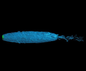
To capture the effect of the submerged cavitator on the flow, the immersed boundary method (Mittal & Iaccarino Reference Mittal and Iaccarino2005; Kim & Choi Reference Kim and Choi2019) is employed in the flow solver (Cui et al. Reference Cui, Yang, Jiang, Huang and Shen2018), wherein an appropriate body force is applied on the grid points near the cavitator surface to enforce the no-slip boundary condition. The immersed boundary method can be applied to resolve solid bodies in Cartesian grids instead of in body-fitted grids, thereby simplifying the algorithm and reducing the computational time. Figure 2 shows a typical instantaneous cavity in our simulation. Several ventilated cavitation components are indicated in the figure, including the interface, which is the air–water boundary, the front part, which is the main body of the cavity, and the closure part, which is the rear portion of the cavity from which air escapes and where the two phases mix violently. To further illustrate these dynamics, a supplementary movie is provided. It offers a real-time visual representation, specifically highlighting the violent mixing process and the escape of air packets from the closure part of the cavity (see supplementary movie available at https://doi.org/10.1017/jfm.2023.431).

Figure 2.

Visualization of a cavity with various components. The isosurfaces of $\psi =0$ (blue) and the disk cavitator (green) are plotted.

2.3. Computational parameters

The $50d_{c}\times 50d_{c}\times 50d_{c}$ (length $\times$ height $\times$ width) computational domain is discretized using a stretched Cartesian mesh grid. The length of the computational domain is enlarged to the maximal possible range according to the available computational resources to ensure that the outlet boundary condition has an insignificant effect on the ventilated cavitation. We conducted three simulations using different mesh grids with various resolutions, which are denoted as $M_{1}$, $M_{2}$ and $M_{3}$. The grids $M_{1}$, $M_{2}$ and $M_{3}$ have $400\times 96\times 96$, $800\times 192\times 192$ and $1600\times 384\times 384$ grid points, respectively. The mesh grid is refined around the cavitator and is coarsened progressively along the $(x-x_{c})/d_{c}<4$ and $(x-x_{c})/d_{c}>18$ directions (figure 3). Table 1 lists the grid resolution in terms of the minimum cell size $\varDelta _{min}$, the time step ${\rm \Delta} t_{f}$, the grid number, the number of cores used for the parallel computing, and the total core-hours spent on the simulations.

Figure 3.

Sketch of the mesh grid $M_{3}$ on the midplane of the computational domain, where the red dashed rectangle indicates the refined mesh region, and the green rectangle denotes the disk cavitator. For illustration purposes, only one of every four grid points in each direction is plotted.

Table 1.

Summary of simulation runs.

The $M_{1}$ simulation was performed until the size of the cavity became statistically stable at approximately $t_{c}=700d_{c}/U_{\infty }$. The simulation was continued for $t_{c}=500d_{c}/U_{\infty }$ to obtain the flow statistics. Then the $M_{2}$ and $M_{3}$ simulations were initialized by interpolating the $M_{1}$ simulation flow field data at $t=t_{c}$ to the mesh grids with higher resolutions.

The flow statistics of the $M_{2}$ and $M_{3}$ simulations are calculated after transient periods $t=3.8d_{c}/U_{\infty }$ and $t=5.2d_{c}/U_{\infty }$, respectively, during which the flows adjust to the statistical stationary status under the new grid resolutions. The flow statistics of the $M_{2}$ and $M_{3}$ simulations are calculated over durations $t=480d_{c}/U_{\infty }$ and $t=440d_{c}/U_{\infty }$, respectively.

The time step is set based on the stability criteria (Ling et al. Reference Ling, Fuster, Tryggvason and Zaleski2019)

(2.12)$$\begin{gather} {\rm \Delta} t\leq{\rm \Delta} t_{conv}=\frac{c\Delta_{min}}{u_{max}}, \end{gather}$$

(2.13)$$\begin{gather}{\rm \Delta} t\leq{\rm \Delta} t_{vis}=\frac{\Delta_{min}^{2}}{6\nu}, \end{gather}$$

where $c$ is the Courant–Friedrichs–Lewy (CFL) number, ${\rm \Delta} t_{conv}$ is the time step restriction for the convection term, and ${\rm \Delta} t_{vis}$ is the time step restriction for the viscous term. Take simulation $M_{3}$ as an example. The CFL number $c$ is set to 0.4, $\varDelta _{min}/d_{c}=0.01$, ${\rm \Delta} t_{conv}\,U_{\infty }/d_{c}=0.005$ and ${\rm \Delta} t_{vis}\,U_{\infty }/d_{c}=0.01$. Therefore, we set the time step as ${\rm \Delta} t=2\times 10^{-3}$ to ensure computational stability. The numerical method and grid resolution selection approach are validated by comparisons with data in the literature and grid convergence tests, and the details are provided in Appendix A.

Ventilated cavitating flows are characterized by several dimensionless parameters, including: the cavitation number $\sigma _{c}=(p_{\infty }-p_{c})/(0.5\rho _{w}U_{\infty }^{2})$, where $p_{\infty }$ and $p_{c}$ are the pressure of the incoming flow and the pressure inside the cavity, respectively; the air entrainment coefficient $C_{q}=Q/(U_{\infty }d_{c}^2)$; the Froude number $Fr=U_{\infty }/\sqrt {gd_{c}}$, where $g$ is the gravitational acceleration; the Reynolds number $Re = \rho _{w} U_{\infty }d_{c}/\mu _{w}$; the blockage ratio $B=d_{c}/D_{T}$, where $D_{T}$ represents the hydraulic diameter of the water tunnel cross-section; and the Weber number $We=\rho _{w} U_{\infty }^{2}d_{c}/\sigma _{T}$, where $\sigma _{T}$ is the surface tension coefficient. Note that the definition of $\sigma$ considers only the ventilation effect, which is consistent with previous studies, e.g. Ahn et al. (Reference Ahn, Jeong, Kim, Shao, Hong and Arndt2017), as the vaporized liquid is negligible compared with the ventilated gas. In this study, we are interested in the scenario in which the gravitational effect is negligible; thus we set $Fr$ to $\infty$. In this case, the flow field is axisymmetric, and the closure mode is RJ. Because most of the cavity has a small curvature and surface tension effects are negligible, $We$ is set to $\infty$. The other dimensionless parameters are set as $C_{q}=0.14$, $Re=1000$ and $B=1.8\,\%$. A relatively small Reynolds number is chosen to resolve all the turbulent eddies in the cavity by the DNS without introducing a turbulence model. Although the Reynolds number is considerably higher ($10^{5}\unicode{x2013}10^{7}$) in practice, the present DNS approach is still a useful research tool that provides insight into the fundamental dynamics of flow physics (Moin & Mahesh Reference Moin and Mahesh1998). In a previous study, we found that $B=1.8\,\%$ is sufficiently small to prevent blockage effects. The density ratio is set to $\rho _{a}/\rho _{w}=0.0012$, and the dynamic viscosity ratio is set to $\mu _{a}/\mu _{w}=0.0154$, which are realistic values for air and water.

3. Flow statistics

Although the simulation is conducted on a Cartesian grid, the data must be transformed from Cartesian coordinates, namely $(x, y, z)$, to cylindrical coordinates, namely $(r, \theta, x)$, to analyse the flow field, which is statistically axisymmetric because $Fr=0$, as explained in § 2.3. The transformation is performed as follows:

(3.1)\begin{equation} r=\sqrt{y^{2}+z^{2}} \end{equation}

and

(3.2)\begin{equation} \theta={\rm tan}^{{-}1}\left(\frac{z}{y}\right). \end{equation}

Finally, $x$ remains the same in both coordinate systems.

The vector components in the cylindrical coordinate system, namely $(f_{r}, f_{\theta }, f_{x})$, can be calculated according to the components in the Cartesian coordinate system, namely $(f_{1}, f_{2}, f_{3})$, as follows:

(3.3)$$\begin{gather} f_{r}=f_{2}\cos(\theta)+f_{3}\sin(\theta), \end{gather}$$

(3.4)$$\begin{gather}f_{\theta}={-}f_{2}\sin(\theta)+f_{3}\cos(\theta), \end{gather}$$

and

(3.5)$$\begin{gather}f_{x}=f_{1}. \end{gather}$$

After the simulation reaches a fully turbulent and statistically steady state, the mean quantity of a variable $f$, denoted as $\bar {f}$, can be determined by averaging over both the azimuthal direction and time as

(3.6)\begin{equation} \bar{f}(x,r)=\frac{1}{2{\rm \pi} (t_{2}-t_{1})}\left(\int_{0}^{2{\rm \pi}}\int_{t_{1}}^{t_{2}} f(r, \theta, x, t)\, {\rm d}t\, {\rm d}\theta\right).\end{equation}

The integration in the azimuthal direction is performed numerically as

(3.7)\begin{equation} \int_{0}^{2{\rm \pi}}f(r,\theta,x,t)\,\mathrm{d}\theta= \frac{\displaystyle \sum_{k=1}^{N_{z}}\sum_{j=1}^{N_{y}}f(x_{i},y_{j}, z_{k})\,H_{r}(r_{jk})}{\displaystyle \sum_{k=1}^{N_{z}} \sum_{j=1}^{N_{y}}H_{r}(r_{jk})},\end{equation}

where $i$, $j$ and $k$ are the indices of discretized grid points in the $x$, $y$ and $z$ directions, and

(3.8)\begin{equation} H_{r}(r_{jk})=\left\{\begin{array}{@{}ll@{}} 1, & |r_{jk}-r|<{\rm \Delta} r/2,\\[2pt] 0, & \text{other area}, \end{array}\right. \end{equation}

with

(3.9)$$\begin{gather} r_{jk}=\sqrt{y_{j}^2+z_{k}^2}, \end{gather}$$

(3.10)$$\begin{gather}{\rm \Delta} r=c({\rm \Delta} x{\rm \Delta} y{\rm \Delta} z)^{1/3}. \end{gather}$$

In the above equations, $c$ is a constant that is set to $1.9$ to ensure that $\sum _{k=1}^{N_{z}}\sum _{j=1}^{N_{y}}H_{r}(r_{jk})>0$ for all considered $r$ values and that $\bar {f}$ is not oversmoothed. Statistical averaging is performed over a duration $80d_{c}/U_{\infty }$, as a fluid particle can travel through the computational domain during this period.

To consider the density difference between the water and gas phases, density-weighted averaging, which is also known as Favre averaging, is employed to analyse the results. The Favre average is expressed as

(3.11)\begin{equation} \tilde{f}=\frac{\overline{\rho f}}{\bar{\rho}}.\end{equation}

The fluctuations are thus defined as

(3.12)\begin{equation} f'=f-\bar{f} \end{equation}

and

(3.13)\begin{equation} f''=f-\tilde{f}.\end{equation}

3.1. Mean flow

Figure 4 shows the contours of the mean volume fraction of water superimposed over the streamlines of the mean flow, which are obtained based on the time and azimuthal averages (3.6). The streamlines indicate the presence of a recirculation zone inside the cavity, in which the air travels forwards near the air–water interface but backwards near the central axis of the cavity. The mean profile of the cavity is defined by the isoline of the mean volume fraction at $\bar {\phi }=0.5$. Figure 5 shows the contours of the mean volume fraction of water and the corresponding isolines at the closure of the cavity. The value of $\phi$ inside the closure region is within the range $0.2\unicode{x2013}0.8$, which implies that the air and water mix violently in this region. Moreover, the contour pattern is concave near the central axis, which is due to the jet flow of the outside water. The underlying physics of this phenomenon is discussed further in the rest of § 3, as well as in §§ 4 and 5.

Figure 4.

Contours of the mean volume fraction of water $\bar {\phi }$ and the streamlines of the mean flow field $\bar {\boldsymbol {u}}$.

Figure 5.

Contours of the mean volume fraction of water, $\bar {\phi }$, and the corresponding isolines in the closure region of the cavity.

The streamwise and radial velocities of the air phase are defined as (Kinzel et al. Reference Kinzel, Lindau and Kunz2009)

(3.14)\begin{equation} u_{x,a}=(1-\phi)u \end{equation}

and

(3.15)\begin{equation} u_{r,a}=(1-\phi) u_{r}, \end{equation}

where $u_{r}$ is the radial velocity, which is calculated according to (3.3). They characterize the streamwise and transverse motions of air inside the cavity, as they equal the local velocities if the position is in the air phase, zero in the water phase, and $(1-\phi )u$ and $(1-\phi )u_{r}$ in grid cells with two phases.

Figures 6(a,b) show $\bar {u}_{a}$ and $\bar {u}_{r,a}$ inside the cavity. Figure 6(a) indicates that forward and backward motions occur inside the cavity in the red-coloured and blue-coloured areas, respectively. Figure 6(b) shows that compared with the streamwise velocity, the radial velocity of the air flow is negligible, except in the regions near the head and rear of the cavity. The $\bar {\phi }=0.5$ contour through the red-coloured region indicates that the air moves outwards and approaches the interface at the head of the cavity before travelling inwards towards the central axis near the rear part of the cavity. These results are consistent with the flow pattern shown in figure 4.

Figure 6.

Contours and profile of the mean air-phase velocities: (a) contours of $\bar {u}_{a}$, (b) profile of $\bar{u}_{a}$ along the central axis, (c) contours of $\bar {u}_{r,a}$, (d) contours of $\bar {u}_{a}$ in the region $4.5<(x-x_{c})/d_{c}<8.0$ and $0< r/d_{c}<1.4$, and (e) contours of $\bar {u}_{a}$ in the region $11.5<(x-x_{c})/d_{c}<14.0$ and $0< r/d_{c}<1$. The black rectangle and green hemisphere in (a,c) denote the cavitator and ventilation source, respectively. The black dashed line corresponds to the isoline of $\bar {\phi }=0.5$. The vertical solid lines in (a,c) indicate the locations where the cross-sectional profiles are plotted in figure 7. The green dashed rectangles correspond to the locations of (d,e).

Figures 6(c,d) display the contours of $\bar {u}_{a}$ in the middle and closure regions of the cavity. Figure 6(c) demonstrates that two flow structures dominate in the middle part of the cavity: the shear layer (SL), corresponding to the red-coloured contour area near the interface, and the recirculation area (RA), corresponding to the blue-coloured area near the streamwise central axis. In the SL, the flow is characterized by high local shear. In the RA, the fluid particles move backwards towards the cavitator and decelerate. Another characteristic flow structure, known as the jet layer (JL), can be observed outside the cavity near the closure region, as depicted in figure 6(e). One branch of the jet moves backwards and re-enters the bubble as a two-phase mixed fluid, while the other jet branch moves forwards into the wake.

The structures of the SL and RA have been discussed in previous studies (Callenaere et al. Reference Callenaere, Franc, Michel and Riondet2001; Spurk Reference Spurk2002; Kinzel et al. Reference Kinzel, Lindau and Kunz2009). To the best of our knowledge, however, no previous studies have investigated the JL in ventilated cavitating flows. Moreover, the relationships between the SL, RA and JL and the turbulent flow in a cavity have not yet been elucidated. In the present study, the roles of these structures in turbulence generation and transport are investigated in § 4. Moreover, in § 5, their relationship with the air leakage and vortex shedding processes is discussed.

Figures 7(a,b) show the mean air-phase velocity profiles of the streamwise and radial components at the streamwise locations marked by the vertical lines in figure 6. Figure 7(a) indicates that the maximum streamwise recirculating velocity, i.e. the maximum negative $\bar {u}_a$, occurs at the central axis of the cavity. Moreover, its magnitude increases along the streamwise direction. The peak of the positive $\bar {u}_a$ occurs near the air–water interface of the cavity. This value increases until the maximum cavity radius at $(x-x_{c})/d_{c}\sim 6$, and then decreases. Figure 7(b) shows that the peak value of the mean radial velocity $\bar {u}_{r,a}$ decreases before this point and then increases with the opposite sign. Furthermore, figure 7 shows that the air-phase streamwise motion dominates the radial component inside the cavity. The air-phase streamwise velocity $u_{x, a}$ is also referred to as the local rate of air entrainment in the literature (Kinzel et al. Reference Kinzel, Lindau and Kunz2009).

Figure 7.

Mean air-phase velocity profiles at different downstream locations: (a) streamwise velocity $\bar {u}_{x, a}$, and (b) radial velocity $\bar {u}_{r, a}$.

Figure 8 shows the distribution of the mean cavitation number $\bar {\sigma }_{c}$ along the central axis. Near the closure region, $\bar {\sigma }_{c}$ decreases suddenly due to the increase in pressure caused by stagnation inside the JL. However, $\bar {\sigma }_{c}$ remains constant inside the cavity.

Figure 8.

Variation in the mean cavitation number along the central axis in the streamwise direction.

3.2. Vortex dynamics

Because of the difficulty in obtaining measurements inside the bubble, only a few experimental studies (e.g. Yoon et al. Reference Yoon, Qin, Shao and Hong2020) on vorticity dynamics in cavities have been conducted. However, vortex dynamics are important in air leakage, air ventilation and turbulence production. In the present paper, characteristic vortex structures and the corresponding vortex dynamics are studied in the various parts of the cavity to elucidate the physical mechanisms in the cavity.

Figure 9 shows the contours of the instantaneous azimuthal vorticity $\omega _{\theta }$ through a midplane in the computational domain. The upper blue region and lower red region indicate two SL structures at the front of the cavity, and the vorticity is generated mainly by the shear between the water and air phases. In the closure region, these two SL structures interact with each other and generate smaller vortex structures. Moreover, some of these small vortices leave the cavity and enter the wake flow. In the RA, i.e. the front part of the cavity, alternating red and blue vortex structures can be observed. Near-cavitator vortices were also observed experimentally by Yoon et al. (Reference Yoon, Qin, Shao and Hong2020). However, these vortices were generated by a different process, namely, the interaction between the injection and reverse flows. The various mechanisms are caused by the differences in the ventilation settings between the present simulation and the experiment by Yoon et al. (Reference Yoon, Qin, Shao and Hong2020). Yoon et al. (Reference Yoon, Qin, Shao and Hong2020) set the direction of the injection flow towards the reversal flow, which caused interactions between the two flows, thus generating vortices. In contrast, in the present simulation, we used a spherical source to ventilate air into the cavity, which does not lead to strong interactions between the ventilated air and the reversal flow. The vortices observed in our simulations are generated mainly in the closure region and convected backwards by the recirculating flow.

Figure 9.

Contours of the instantaneous vorticity component $\omega _{\theta }$ on a midplane in the computational domain.

The square of the vorticity, $\zeta =(\omega _{x}^{2}+\omega _{y}^{2}+\omega _{z}^{2})/2$, represents the enstrophy per unit mass. In this work, this quantity is employed to evaluate the intensity of vortex structures to study the vortex dynamics in the cavity. Specifically, the enstrophy is decomposed into two parts: $\zeta =\zeta _{x}+\zeta _{yz}$, where $\zeta _x=\omega _{x}^{2}/2$ is the streamwise enstrophy caused by spiral motions in the cross-sectional plane, and $\zeta _{yz}=\omega _{yz}^{2}=(\omega _{y}^{2}+\omega _{z}^{2})/2$, which denotes the transverse enstrophy and is related mainly to shear motion in the $x\unicode{x2013}r$ plane.

Figure 10 shows the contours of the mean enstrophy $\bar {\zeta }$ and its two components $\bar {\zeta }_{x}$ and $\bar {\zeta }_{yz}$. Figure 10(a) indicates that strong vortical motions occur in the SL in the front and closure regions of the cavity. Figure 10(b) shows that strong streamwise vorticity occurs only in the closure region. Moreover, figure 10(c) suggests that strong transverse vortices occur not only in the closure region of the cavity but also in the SL in the front part. In the closure region, the transverse enstrophy is larger than the streamwise enstrophy. The dominance of transverse vortical motions inside the cavity is attributed to the strong shear at the air–water interface. The strong streamwise vortical motion in the closure region suggests that the flow in this area transitions to a more three-dimensional and isotropic state due to the strong mixing between the two fluid phases in this region.

Figure 10.

Contours of the mean enstrophy and its components: (a) $\bar {\zeta }$, (b) $\bar {\zeta }_{x}$, and (c) $\bar {\zeta }_{yz}$. The dashed line represents the isoline of $\bar {\phi }=0.5$. The vertical solid lines indicate the locations of the cross-sectional profiles in figure 11.

To elucidate the underlying physics of the vortex dynamics in the cavity, the mean enstrophy distributions along the radial direction are examined. Figure 11 shows the profiles of the mean enstrophy ($\bar \zeta$) and its two components ($\bar \zeta _x$ and $\bar \zeta _{yz}$) at different streamwise locations (see the vertical lines in figure 10) inside the cavity. The peak value of the transverse enstrophy $\bar \zeta _{yz}$ occurs near the interface of the cavity, where the shear effect is strong. The peak $\bar \zeta _{yz}$ remains approximately constant at the front (comparing $(x-x_{c})/d_{c}=2, 4, 6, 8, 10$) and becomes larger in the closure region ($(x-x_{c})/d_{c}=12$). However, the peak value of the streamwise enstrophy increases along the downstream direction until the closure region. The above variations occur because the transverse vortical motion is caused by the two-phase shear effect, which maintains a nearly constant strength in the SL in the front region, while the streamwise vortical motion is ascribed to the development of turbulence, which gradually intensifies along the streamwise direction.

Figure 11.

Profiles of the mean enstrophy and its components at different downstream locations: (a) $\bar \zeta$, (b) $\bar \zeta _{x}$, and (c) $\bar \zeta _{yz}$.

To study the vortex dynamics and identify the governing mechanism during the cavity–turbulence interaction, we examine the enstrophy budget equation, which is expressed as

(3.16)\begin{equation} \frac{\partial (\frac{1}{2}\omega_{i}\omega_{i})}{\partial t}+ \frac{\partial (\frac{1}{2}\omega_{i}\omega_{i}u_{j})}{\partial x_{j}}= \underbrace{\omega_{i}\omega_{j}\,\frac{\partial u_{i}}{\partial x_{j}}}_{W_{s}}+ \underbrace{\frac{1}{\rho^{2}}\,\omega_{i}\epsilon_{ijk}\, \frac{\partial \rho}{\partial x_{j}}\,\frac{\partial p}{\partial x_{k}}}_{W_{b}}+ \underbrace{\omega_{i}\epsilon_{ijk}\,\frac{\partial}{\partial x_{j}}\left(\frac{1}{\rho}\,\frac{\partial\sigma_{kl}}{\partial x_l}\right)}_{W_{v}}.\end{equation}

This equation is derived from the variable-density Navier–Stokes equations (2.1). The vortex dynamics is governed by three terms, namely, the stretching effect term $W_{s}$, the baroclinic effect term $W_{b}$, and the viscous effect term $W_{v}$ in (3.16). These effects are displayed in figure 12. The stretching and baroclinic effects are responsible for generating enstrophy, while the viscous term dissipates enstrophy. Figure 12 shows that all three effects are weak at the front part of the cavity and strong in the closure region.

Figure 12.

Contours of the mean budget terms in the enstrophy equation (3.16): (a) the stretching effect term $\overline {W_{s}}$, (b) the baroclinic effect term $\overline {W_{b}}$, and (c) the viscous effect term $\overline {W_{v}}$. The dashed line indicates the isoline of $\bar {\phi }=0.5$. The vertical solid lines indicate the locations of the cross-sectional profiles in figure 13.

Moreover, we obtained the radial distributions of the three budget terms. Figure 13 shows the profiles of these three terms at different downstream locations. The magnitudes of the baroclinic and viscous terms are comparable and dominate the stretching term. The baroclinic effect plays an essential role in the production of enstrophy, while the baroclinic and viscous terms nearly cancel one another. In addition, the peak values of the three terms occur near the air–water interface in the cavity, and tend to increase along the downstream direction due to the increasing intense interaction between the air and water phases.

Figure 13.

Profiles of the mean budget terms in the enstrophy equation (3.16) at different streamwise locations: (a) stretching effect term $\bar {W}_{s}$, (b) baroclinic effect term $\bar {W}_{b}$, and (c) viscous effect term $\bar {W}_{v}$.

3.3. Reynolds stresses

Reynolds stresses play important roles in momentum transport and the interaction between turbulent fluctuations and the mean flow, which is responsible for the production of TKE. Previous studies have investigated Reynolds stress distributions in sheets and attached cavitation processes (Gopalan & Katz Reference Gopalan and Katz2000; Iyer & Ceccio Reference Iyer and Ceccio2002). However, less is known about the Reynolds stress distribution in artificial ventilated cavitation processes. The present simulation data can be used to address this knowledge gap. In an air–water two-phase flow, Reynolds stresses are defined with a variable density. The Favre-averaged momentum equations for a variable-density flow are written as

(3.17) \begin{equation} \frac{\partial(\bar{\rho} \tilde{{u_{i}}})}{\partial t}+ \frac{\partial(\bar{\rho}\tilde{u}_{i}\tilde{u}_{j})}{\partial x_{j}}=-\frac{\partial \bar{p}}{\partial x_{i}} - \frac{\partial \bar{\rho}\,\widetilde{{u_{i}''u_{j}''}}}{\partial x_{j}} + \frac{\partial{\bar{\sigma}_{ij}}}{\partial x_{j}},\end{equation}

where

(3.18)\begin{equation} \tau^{R}_{ij}={-}\bar{\rho}\,\widetilde{u_{i}''u_{j}''}, \end{equation}

is the Reynolds stress tensor. In RANS simulations, the Reynolds stresses need to be closed in terms of the mean quantities. To develop models to describe cavitating flows in the future, we study the structural characteristics and spatial distribution of the Reynolds stress. Because of the axisymmetry of the cavitating flow under investigation, the Reynolds stress components $\tau ^{R}_{x\theta }$ and $\tau ^{R}_{r\theta }$ are zero. Therefore, only the four independent components of the Reynolds stress tensor, namely, $\tau ^{R}_{xx}$, $\tau ^{R}_{rr}$, $\tau ^{R}_{\theta \theta }$ and $\tau ^{R}_{xr}$, are considered in the discussions below.

Figure 14 shows the contours of the four components of the Reynolds stress tensor. To visualize the distributions more clearly, we also depict profiles of the Reynolds stress components at several downstream locations in figure 15. As shown in the figures, in the front part of the cavity, $\tau ^{R}_{xx}$ is the dominant component of the Reynolds stress, while the other components are negligibly small. Figure 15(a) indicates that the maximum magnitude of $\tau ^{R}_{xx}$ occurs at the air–water interface, where strong interactions occur between the two phases, and the peak value increases in the downstream direction. Figures 15(b,c) show that $\tau ^{R}_{rr}$ and $\tau ^{R}_{\theta \theta }$ are similar in the closure region of the cavity, indicating that the flow becomes more isotropic in this region. Moreover, figure 14(d) shows that $\tau ^{R}_{xr}$ is mostly positive. The quadrant analysis in Appendix B shows that the positive $\tau ^{R}_{xr}$ component is associated with the dominant contributions of the $Q_{2}$ and $Q_{4}$ quadrants over the $Q_{1}$ and $Q_{3}$ quadrants of the Reynolds shear stress. Similarly, the peak value of $\tau ^{R}_{xr}$ tends to occur near the two-phase interface, and increases along the streamwise direction.

Figure 14.

Contours of the Reynolds stress components: (a) $\tau ^{R}_{xx}$, (b) $\tau ^{R}_{rr}$, (c) $\tau ^{R}_{\theta \theta }$, and (d) $\tau ^{R}_{xr}$. The black dashed line denotes the isoline of $\bar {\phi }=0.5$. The vertical lines indicate the locations where the cross-sectional profiles are plotted in figure 15.

Figure 15.

Profiles of the Reynolds stress components at different streamwise locations: (a) $\tau ^{R}_{xx}$, (b) $\tau ^{R}_{rr}$, (c) $\tau ^{R}_{\theta \theta }$, and (d) $\tau ^{R}_{xr}$.

In summary, the following conclusions can be drawn according to the Reynolds stress analysis. First, the peak value of the streamwise component of the Reynolds stress occurs near the air–water interface, and this component dominates the other components in most of the cavity. Second, the Reynolds stresses become stronger near the closure region, and the diagonal components are comparable, indicating that the flow becomes more turbulent and isotropic in this region.

4. Turbulence and energy budget

The TKE dynamics is particularly important in turbulence modelling. In the present multiphase flow study, based on the Favre average and the fluctuations defined in (3.11) and (3.13), the TKE is defined as

(4.1)\begin{equation} q=\tfrac{1}{2}u_{i}''u_{j}''. \end{equation}

Turbulence occurs predominantly in the closure region and tends to be concentrated in the JL structure. Figure 16 plots the contours of the Favre-averaged TKE $\tilde {q}$ in this region. The TKE isolines qualitatively resemble a group of ellipses. Their centre occurs near the stagnation point in the JL, where the TKE obtains its peak value. The strong turbulence is caused by the violent mixing of air and water in this region. To further evaluate the isotropy of turbulence in the cavity, we consider the TKE fraction function (Liu & Xiao Reference Liu and Xiao2016), which is expressed as

(4.2) \begin{equation} f_{q}=\frac{2\,\widetilde{u_{1}'' u_{1}''}}{\widetilde{u_{2}''u_{2}''}+ \widetilde{u_{3}''u_{3}''}}. \end{equation}

This fraction is twice the ratio of the TKE associated with streamwise fluctuations to that associated with transverse fluctuations. If $f_q\sim 1$, then the turbulence reaches an approximately isotropic state. Figure 17 displays the contours of $f_{q}$ in the same closure region as shown in figure 16. The peaks occur near the shear layer and the stagnation point in the JL. The peak values are larger than 3.0, which indicates that the streamwise component of the TKE is considerably stronger than the transverse component of the TKE in both SL and JL.

Figure 16.

Contours of the Favre-averaged TKE, $\tilde {q}$. The green solid lines are the isolines of $\tilde {q}$, and the black dashed line corresponds to the isoline of $\bar {\phi }=0.5$.

Figure 17.

Contours of the TKE fraction function, $f_{q}$. The green solid lines are the isolines of $f_{q}$, and the black dashed line corresponds to the isoline of $\bar {\phi }=0.5$.

To elucidate the mechanisms responsible for generating and transporting TKE, we examine its budget equation based on density-weighted averaging as follows:

(4.3)\begin{equation} 0=\underbrace{-\frac{\partial}{\partial x_{j}}(\bar{\rho}\tilde{q}\tilde{u_{j}})}_{\varPi_{c}} \underbrace{{}-\overline{\rho u''_{i}u''_{j}}\, \frac{\partial \tilde{u_{i}}}{\partial x_{j}} }_{\varPi_{d}}\underbrace{{}-\frac{\partial}{\partial x_{j}} \left[\overline{u''_{j}\left(\frac{1}{2}\,\rho u''_{i}u''_{i} \right)}\right] }_{\varPi_{tt}} \underbrace{{}-\overline{u''_{i}\,\frac{\partial p}{\partial x_{i}}} }_{\varPi_{p}} +\underbrace{\frac{\partial}{\partial x_{j}} \left(\overline{u''_{i}\sigma'_{ij}}\right) }_{\varPi_{vt}} -\underbrace{\overline{\sigma'_{ij}\, \frac{\partial u_{i}''}{\partial x_{j}}}} _{\epsilon}, \end{equation}

where $\varPi _{c}=-\partial (\bar {\rho } \tilde {q}\tilde{u_{j}})/\partial x_{j}$ is the mean flow advective transport, $\varPi _{d}=-\overline {\rho u''_{i}u''_{j}}\, \partial \tilde{u_{i}}/\partial x_{j}$ is the production, $\varPi _{tt}=-\partial [\overline {u''_{j}(\frac 12\rho u''_{i}u''_{i})}]/\partial x_{j}$ is the turbulent transport, $\varPi _{p}=-\overline {u''_{i}\,\partial p/\partial x_{i}}$ is the pressure transport, $\varPi _{vt}=\partial (\overline {u''_{i}\sigma '_{ij}})/\partial x_{j}$ is the viscous transport, and $\epsilon =\overline {\sigma '_{ij}\,\partial u_{i}''/\partial x_{j}}$ is the viscous dissipation. The numerical results show that $\varPi _{tt}$ and $\varPi _{vt}$ are negligible (not plotted here). Therefore, in the discussions below, we focus on the remaining terms.

Figure 18 shows the contours of the dissipation term $\epsilon$ in the closure region, where the TKE is the largest (figure 16). The contour pattern is qualitatively similar to that of the TKE, especially in the JL region, as depicted in figure 16. The maximum dissipation occurs in the vicinity of the stagnation point. As is well known, $\epsilon$ is always positive and transforms TKE into internal energy.

Figure 18.

Contours of the viscous dissipation term $\epsilon$. The green solid lines are the isolines of $\epsilon$, and the black dashed line corresponds to the isoline of $\bar {\phi }=0.5$.

Figure 19 displays the contours of the advective transport component $\varPi _{c}$. The blue contour in the SL indicates that energy is convected out of this region by the mean flow, and the red contour in the JL region suggests that the mean flow convects the energy into this area. This TKE transport phenomenon can be explained as follows. We can rewrite $\varPi _{c}$ as $\varPi _{c}=-\bar {\rho }\tilde {u}_{k}\,\partial q/\partial x_{k}=-\boldsymbol {v}\boldsymbol {\cdot }\boldsymbol {\nabla } q$. Additionally, figure 19 displays the TKE isolines. Here, $\boldsymbol {\nabla } q$ is normal to these isolines and points towards the stagnation point. The streamlines are plotted as green lines with arrows. In the SL, the mean flow moves towards the stagnation point, leading to negative $\varPi _{c}$ ($-\boldsymbol {v}\boldsymbol {\cdot }\boldsymbol {\nabla } q<0$). Thus TKE is convected out of the SL region. However, in the JL, the mean flow moves away from the stagnation point, leading to positive $\varPi _{c}$ ($-\boldsymbol {v}\boldsymbol {\cdot }\boldsymbol {\nabla } q>0$). Therefore, TKE is convected into the two JL branches.

Figure 19.

Contours of the advective transport term $\varPi _{c}$. The green lines with arrows indicate the streamlines, the black dashed line corresponds to the isoline of $\bar {\phi }=0.5$, and the black solid lines represent the TKE isolines.

The contours of the TKE production term $\varPi _{d}$ are plotted in figure 20(a), which shows different characteristics in the SL and JL regions. The positive contour values in the red-coloured region indicate that kinetic energy is transferred from the mean flow to the turbulent flow by $\varPi _{d}$ in the SL, while the negative contour values in the blue-coloured region indicate that energy is transferred in the reverse direction. To elucidate the physical mechanism underlying this energy transfer process, we decompose $\varPi _{d}$ into three components:

(4.4)\begin{equation} \varPi_{d}={-}\overline{\rho u_{i}''u_{j}''}\, \frac{\partial \tilde{u_{i}}}{\partial x_{j}}= \varPi_{dx}+\varPi_{dt}+\varPi_{ds}, \end{equation}

where $\varPi _{dx}=-\overline {\rho u_{1}''u_{1}''}\,\partial \tilde{u_{1}}/\partial x_{1}$ represents the production due to streamwise stretching effects, $\varPi _{dt}=-(\overline {\rho u_{2}''u_{2}''}\,\partial \tilde{u_{2}}/\partial x_{3}+\overline {\rho u_{3}''u_{3}''}\,\partial \tilde{u_{3}}/\partial x_{3})$ is the production due to the transverse motion, and $\varPi _{ds}=-(\overline {\rho u_{1}''u_{2}''}\,(\partial \tilde{u_{1}}/\partial x_{2}+\partial \tilde{u_{2}}/\partial x_{1})+\overline {\rho u_{3}''u_{1}''}\,(\partial \tilde{u_{3}}/\partial x_{1}+\partial \tilde{u_{1}}/\partial x_{3})$ is the production due to shear effects. Figure 20(b) shows that $\varPi _{dx}$ is negative in both the SL and JL. Figure 20(c) indicates that $\varPi _{dt}$ is positive and concentrated in the JL. Figure 20(d) shows that $\varPi _{ds}$ is mainly positive and concentrated in the SL. Note that $\varPi _{d}$ is positive in the SL and negative in the JL. Therefore, $\varPi _{ds}$ dominates in the SL, while $\varPi _{dx}$ dominates in the JL. To further assess the relative importance of the above terms, we calculate the fraction functions of the magnitudes of different terms as

(4.5)$$\begin{gather} f_{dx}=|\varPi_{dx}|/(|\varPi_{dx}|+|\varPi_{dt}|+|\varPi_{ds}|), \end{gather}$$

(4.6)$$\begin{gather}f_{dt}=|\varPi_{dt}|/(|\varPi_{dx}|+|\varPi_{dt}|+|\varPi_{ds}|), \end{gather}$$

and

(4.7)$$\begin{gather}f_{ds}=|\varPi_{ds}|/(|\varPi_{dx}|+|\varPi_{dt}|+|\varPi_{ds}|).\end{gather}$$

In both the SL and JL, compared with $f_{dx}$ and $f_{ds}$, $f_{dt}$ is negligible (not plotted). The contours of $f_{dx}$ and $f_{ds}$ are depicted in figures 21(a,b): $f_{dx}$ is concentrated in the JL, while $f_{ds}$ dominates in the SL. These results can be explained by the distributions of the Reynolds stress and mean strain rate in the closure region of the cavity. In the SL, the shear effect leads to a positive and strong $\partial \tilde {u}_{x}/\partial r$. Moreover, the Reynolds stress $\tau ^{R}_{xr}$ is positive and non-negligible. Hence the TKE production rate is dominated by the positive $\varPi _{ds}$ component. However, in the two JL branches, the jet flow increases the stretch-strain rate components, i.e. the jet flow generates negative $\partial \tilde {u}_{r}/\partial r$ and positive $\partial \tilde {u}_{x}/\partial x$ components with large magnitudes.

Figure 20.

Contours of the TKE production term and its components: (a) $\varPi _{d}$, (b) $\varPi _{dx}$, (c) $\varPi _{dt}$, and (d) $\varPi _{ds}$. The black dashed line represents the isoline of $\bar {\phi }=0.5$.

Figure 21.

Contours of the fraction functions of the components of $\varPi _{d}$: (a) $f_{dx}$, and (b) $f_{ds}$. The black dashed line represents the isoline of $\bar {\phi }=0.5$.

Note that the streamwise Reynolds stress dominates in the JL (see figure 17). Consequently, the TKE production rate is dominated by the negative $\varPi _{dx}$ component in the JL because of the negative $\tau _{xx}^{R}$ and positive $\partial \tilde {u}_{x}/\partial x$.

The TKE pressure transport term can be decomposed into three parts:

(4.8)\begin{equation} \varPi_{p}={-}\overline{u_{k}''\,\frac{\partial p}{\partial x_{k}}} =\varPi_{pm}+\varPi_{pt}+\varPi_{pd}, \end{equation}

where $\varPi _{pm}=-\overline {u_{k}''}\,\partial \bar {p}/\partial x_{k}$ is the transport due to the mean pressure gradient, $\varPi _{pt}=-\partial \overline {p'u_{k}''}/\partial x_{k}$ is the transport due to the pressure–velocity fluctuation correlation, and $\varPi _{pd}=\overline {p'\,\partial u_{k}''/\partial x_{k}}$ is the transport due to the dilatation effect. Note that $\varPi _{pd}$ decreases because of the incompressibility of the two phases. The contours of $\varPi _{pm}$ and $\varPi _{pt}$ are displayed in figures 22 (a,b). The figure shows that $\varPi _{pm}$ is positive in both the SL and JL, which enhances the TKE in the closure region of the cavity. On the other hand, $\varPi _{pt}$ is largely negative in the SL and tends to transport TKE from the SL region to the JL region.

Figure 22.

Contours of the pressure transport terms: (a) $\varPi _{pm}$, and (b) $\varPi _{pt}$. The black dashed line denotes the isoline of $\bar {\phi }=0.5$.

To summarize § 4, figure 23 illustrates the energy transfer processes among the turbulent flows in the SL and JL regions and the mean flow. The aforementioned results show that the SL and JL structures have distinct characteristics during TKE generation and transport. In the SL, the TKE is increased by the production term due to the shear effect term $\varPi _{ds}$, while in the JL structure, the TKE decreases due to the streamwise stretching effect term $\varPi _{dx}$. The pressure transport term $\varPi _{pm}$ tends to enhance the TKE in both the JL and SL. Moreover, the mean flow advective transport term $\varPi _{c}$ and pressure transport term $\varPi _{pt}$ are conducive to transporting TKE from the SL to the JL.

Figure 23.

Schematic of the energy transport among the mean flow, SL turbulent flow and JL turbulent flow.

5. Air leakage and vortex shedding

In ventilated cavitation, some air escapes from the cavity through the closure part, where violent flow mixing between water and air occurs. Wu et al. (Reference Wu, Liu, Shao and Hong2019) conducted experiments and used particle image velocimetry to study quantitatively the gas leakage process that occurred in the RJ and TV closure modes. Moreover, they discussed the variation in gas leakage during the transition between the RJ and TV modes. Their results indicated that gas leakage occurs due to interactions between the internal and external flows. According to the present simulation results, we made several observations to elucidate the flow characteristics and dynamics in the RJ closure region of the cavity.

First, the simulation data indicate that the air leakage process in the closure region has a one-to-one correspondence with the vortex shedding process, as shown by the instantaneous visualization of the flow. Previous studies (Shao et al. Reference Shao, Karn, Ahn, Arndt and Hong2017; Karn, Arndt & Hong Reference Karn, Arndt and Hong2016) have shown that the RJ mode leaks gas via toroidal-like vortices. However, these works did not connect the gas leakage to the vortex shedding process. Figures 24(a,b) plot the isosurfaces of the VOF function $\phi =0.5$ and the second invariant of the strain rate tensor $Q=2$, with the former coloured according to the magnitude of the pressure, and the latter coloured according to the magnitude of $\phi$. The leakage air–water interface exhibits the same pattern as the vortex structures characterized by $Q$ (Haller Reference Haller2005).

Figure 24.

Instantaneous structures of air leakage and vortex shedding in the closure region of the cavity. (a) Isosurface of $\phi =0.5$, which is coloured according to the magnitude of the pressure. (b) Isosurface of the second invariant of the strain rate tensor ($Q=2$), which is coloured according to the magnitude of $\phi$.

Furthermore, only a few previous laboratory studies (Karn et al. Reference Karn, Arndt and Hong2016; Wu et al. Reference Wu, Liu, Shao and Hong2019) identified the location where the air pockets leave the cavity and the associated vortex shedding. From our simulation result, flow visualization shows that air leakage and vortex shedding occur within the JL structure in the closure region. The colours in figure 24(a) illustrate the pressure distribution on the surface of the cavitation bubble. The disconnection and breakup of the leaked air flow structures from the body of the cavity occur near the high-pressure region, which corresponds to the stagnant region inside the JL structure. The vortex structures in figure 24(b) are coloured according to the value of $\phi$ on the isosurface. The results indicate that vortex tubes and rings occur in the violent air–water mixing region, i.e. the JL region.

Moreover, we observe that the air leakage and vortex shedding processes in the closure region of the cavity are not random, and these processes exhibit semi-periodic patterns with intrinsic characteristic frequencies. Few previous experimental works have investigated the spectra and oscillation patterns of the closure modes due to measurement limitations. Jiang, Shao & Hong (Reference Jiang, Shao and Hong2018) conducted a spectral analysis of the cavity length but did not find a dominant oscillation frequency. In the present study, our three-dimensional simulation results illustrate more details about the oscillations within the different structures in the closure mode.

To investigate the relationship between the vortex shedding and air leakage processes, we employ a temporal Fourier transform to obtain the frequency spectra of the radial velocity $E(u_{r})$ and the VOF function $E(\varPhi )$. The results for $10<(x-x_{c})/d_{c}<15$ along the central axis are shown in figure 25. Figures 25(a) and 25(b) both indicate a significant characteristic frequency, namely $St\approx 0.1$, where the spectra reach their local peaks, indicating that the air leakage and vortex shedding processes share the same characteristic frequency. Moreover, the spectra are more concentrated in the $12.5<(x-x_{c})/d_{c}<14$ region, where the turbulent mixing between the air and water is violent, which contributes to the strong turbulence within this region.

Figure 25.

Frequency spectra of the radial velocity $u_{r}$ and VOF function $\phi$ along the central axis: (a) $\log _{10}(E(u_{r}))$, and (b) $\log _{10}(E(\phi ))$.

The air leakage frequency can also be quantified by defining the total air volume as a function of time in a fixed control volume (CV) bounded by $12.5<(x-x_{c})/d_{c}<14$ and $r/d_{c}<0.8$. The total volume of air $V_{a}(t)$ in the CV is expressed as

(5.1)\begin{equation} V_{a}(t)=\int_{\boldsymbol{x}\in CV} \phi(\boldsymbol{x},t)\, {\rm d}\kern0.06em \boldsymbol{x}.\end{equation}

We then define the following normalized autocorrelation function for $V_{a}$:

(5.2)\begin{equation} R_{V}({\rm \Delta} t)=\frac{\displaystyle \int_{0}^{T}V_{a}(t)\,V_{a}(t+{\rm \Delta} t)\, {\rm d}t}{\displaystyle \int_{0}^{T} V_{a}(t)\,V_{a}(t)\, {\rm d}t}. \end{equation}

Figure 26 shows $R_{V}({\rm \Delta} t)$ versus the time interval ${\rm \Delta} t$, normalized by $d_c$ and $U_\infty$. A peak occurs at ${\rm \Delta} t=11.1d_{c}/U_{\infty }$, which corresponds to the Strouhal number $St=0.09$. This value is close to the peak in the frequency spectra of the radial velocity and VOF function (figure 25). In other words, the air leakage and vortex shedding processes occur at the same frequency, and the two processes are strongly correlated in the closure region in ventilated cavitating flows.

Figure 26.

Normalized autocorrelation function of the bubble volume in the region $12.5< (x-x_{c})/d_{c}<14$, $r/d_{c}<0.8$.

In summary, figures 24–26 demonstrate several properties about the air leakage and vortex shedding processes. First, the generation of vortex structures is associated with the leakage of air bubbles. Both processes occur in the stagnant high-pressure region with violent turbulent mixing between the air and water phases. Second, the vortex shedding in the closure region shows a semi-periodic pattern, and an intrinsic characteristic frequency can be observed in the energy spectra. Third, the air leakage and vortex shedding processes share the same characteristic frequency. Based on the above results, we summarize the air leakage and vortex shedding processes in the closure region of the cavity in the sketch in figure 27. The underlying mechanism can be described as follows. Air is convected forwards through the SL and then terminates, which is accompanied by the generation of vorticity in the SL, as shown by Part 1 in the figure. Due to the constant ventilation from the front part of the cavity, the air cannot remain in the end of the SL region and thus moves into the JL in the closure region, where the air and water are fully mixed, as shown by Part 2 in figure 27. Finally, the air leaks and exits the cavity, generating complex vortex structures that are convected downstream, as depicted in Part 3.

Figure 27.

Schematic of the air leakage and vortex shedding processes. Part 1: vorticity is generated in the SL and convected to the end of the cavity. Part 2: the air in the JL in the cavity continues to convect. Part 3: the air leaks accompanied by the formation of complex large-scale vortex structures.

6. Spectral proper orthogonal decomposition analysis of coherent structures

In this section, we employ the SPOD method (Towne et al. Reference Towne, Schmidt and Colonius2018) to extract and analyse the coherent structures near the closure region of the ventilated cavitating flow. To perform the SPOD analysis, $N_{s}$ snapshots of the flow field $\boldsymbol {q}$ acquired at constant time intervals are decomposed into a set of blocks along the temporal direction as $\boldsymbol {Q}=[\boldsymbol {q}^{(1)}, \boldsymbol {q}^{(2)},\ldots,\boldsymbol {q}^{(i)},\ldots, \boldsymbol {q}^{(N_{freq})}]$, where $i$ is the index of the block, $\boldsymbol {q}=[\boldsymbol {u}_{x}, \boldsymbol {u}_{r}, \boldsymbol {u}_{\theta }]$ is the vector of the velocity components in cylindrical coordinates, and $N_{freq}$ is the number of snapshots in each block (Nidhan et al. Reference Nidhan, Schmidt and Sarkar2022). To improve our spectral analysis, we include $N_{ovl}$ overlapping snapshots between neighbouring blocks, following the treatment in Schmidt & Colonius (Reference Schmidt and Colonius2020). Therefore, the total number of blocks after this decomposition can be calculated as

(6.1)\begin{equation} N_{blk}=\frac{N_{s}-N_{ovl}}{N_{freq}-N_{ovl}}.\end{equation}

Then a temporal Fourier transform is performed in each block to obtain the projections in the frequency domain as

(6.2)\begin{equation} \boldsymbol{q}^{(j)}(x,r,\theta,t)=\varSigma_{\omega}\, \hat{\boldsymbol{q}}^{(j)}_{\omega}(x,r,\theta)\, {\rm e}^{{\rm i}\omega t},\end{equation}

where ${\rm i}$ is the imaginary unit, and $\omega =2{\rm \pi} \,St$ is the angular frequency, which is calculated according to the Strouhal number $St=d_{c}f/U_{\infty }$. The obtained ensemble of $N_{blk}$ blocks with frequency $\omega$ is denoted as $\boldsymbol {Q}_{\omega }=[\hat {\boldsymbol {q}}^{(1)}_{\omega }, \hat {\boldsymbol {q}}^{(2)}_{\omega },\ldots, \hat {\boldsymbol {q}}^{(N_{freq})}_{\omega }]$. After the Fourier transform, we calculate the SPOD eigenvalues and eigenvectors corresponding to the frequency $\omega$ via eigenvalue decomposition as

(6.3)\begin{equation} \hat{\boldsymbol{Q}}_{\omega}^{*}\boldsymbol{W} \hat{\boldsymbol{Q}}_{\omega}\boldsymbol{\varPsi}_{\omega}= \boldsymbol{\varPsi}_{\omega}\boldsymbol{\varLambda}_{\omega},\end{equation}

where $\boldsymbol {W}$ is a weighting matrix, and $\boldsymbol {\varLambda }_{\omega }={\rm diag} (\lambda _{\omega }^{(1)},\lambda _{\omega }^{(2)}, \ldots,\lambda _{\omega }^{(N_{blk})})$ is a diagonal matrix containing the eigenvalues ranked according to decreasing energy from $j=1$ to $N_{blk}$. The $j$th SPOD mode $\varPhi ^{(j)}_{\omega }$ is computed as

(6.4)\begin{equation} \hat{\boldsymbol{\varPhi}}_{\omega}=\hat{\boldsymbol{Q}}_{\omega} \boldsymbol{\varPsi}_{\omega}(\boldsymbol{\varLambda}_{\omega})^{{-}1/2}. \end{equation}

An energy-based inner product is employed to compute the eigenvalues and eigenvectors by defining the weight matrix $\boldsymbol {W}$ as a trapezoidal integration matrix. Thus the norm can be calculated as

(6.5)\begin{equation} \hat{\boldsymbol{Q}}_{\omega}^{*}\boldsymbol{W} \hat{\boldsymbol{Q}}_{\omega}=\int\!\int\!\int_{D} \hat{\boldsymbol{Q}}_{\omega}^{*}\,{\rm diag} (1,1,1)\,\hat{\boldsymbol{Q}}_{\omega} {r}\,{\rm d}{r}\,{\rm d}\kern0.06em {x}\,{\rm d}\theta, \end{equation}

where $D$ is the domain of interest. More details on the SPOD formulation can be found in Towne et al. (Reference Towne, Schmidt and Colonius2018) and Nidhan et al. (Reference Nidhan, Schmidt and Sarkar2022).

For the SPOD analysis in the present work, we use $N_{s}=4096$ consecutive snapshots of the plane at $z=0$ spanning $9.5<(x-x_{c})/d_{c}<15.5$ and $0<(y-0.5L_{y})/d_{c}<1.3$, which includes the closure region of the ventilated cavity. The time interval for the sampled snapshots is ${\rm \Delta} t d_{c}/U_{\infty }=0.1$. We select the number of frequencies as $N_{freq}=512$, and implement a $50\,\%$ overlap between blocks, i.e. $N_{ovl}=256$, to balance improved spectral convergence with reduced spectral entanglement between each window in the Fourier transform. Each data block is multiplied by a Hamming window function before the Fourier transform to effectively reduce errors due to spectral leakage (Schmidt & Colonius Reference Schmidt and Colonius2020). To study the variation in the eigenspectral features at different locations, we perform SPOD analyses in four consecutive domains, $D_{1}$, $D_{2}$, $D_{3}$ and $D_{4}$, which are shown in figure 28.

Figure 28.

Contours of the mean volume fraction of water $\bar {\phi }$ and the streamlines of the mean flow field near the closure region. The four subdomains $D_{1}$, $D_{2}$, $D_{3}$ and $D_{4}$, and the whole domain $D_{t}$, for the SPOD analyses are shown. The black dashed line is the isoline of $\bar {\phi }=0.5$.

We start our analysis of the SPOD modes by studying their relative contributions to the fluctuation energy. Figure 29(a) shows the cumulative fraction of energy, $C_{j}(n)$, as a function of the SPOD modal index $n$ in the four downstream domains $D_{1}$, $D_{2}$, $D_{3}$ and $D_{4}$, which is computed as

(6.6)\begin{equation} C_{j}(n) =\frac{\displaystyle \sum_{i=1}^{n}\sum_{s=St_{min}}^{St_{max}} \lambda_{s}^{(i)}(D_{j})}{\displaystyle \sum_{i=1}^{N_{blk}} \sum_{s=St_{min}}^{St_{max}}\lambda_{s}^{(i)}(D_{j})}.\end{equation}

A comparison of the curves among the different subdomains indicates that the relative energies contributed by the leading SPOD modes increase with the downstream distance. In addition, we observe that the curves for $D_{1}$ and $D_{2}$ essentially collapse onto a single curve, whereas the curves for $D_{2}$ and $D_{3}$ differ considerably, indicating that a transition occurs between $D_{2}$ and $D_{3}$. This result is consistent with our observation in figure 25 that $D_{3}$ contains the region where the air and water mix violently and the turbulence intensity is strong. Moreover, figure 29(a) demonstrates that the first SPOD mode contributes a significant fraction of the total energy, contributing approximately $60\,\%$ of the energy in $D_{1}$ and $D_{2}$, and approximately $70\,\%$ and $80\,\%$ of the energy in $D_{3}$ and $D_{4}$, respectively. These results indicate low-rank behaviours, which are used to describe scenarios in which the physical mechanism associated with the leading mode dominates (Schmidt et al. Reference Schmidt, Towne, Rigas, Colonius and Brès2018).

Figure 29.

Cumulative fraction of energy in different domains, $C_{j}$: (a) as a function of the modal index $n$; and (b) as a function of $St$. The plots are shown for the four considered domains, namely $D_{1}$, $D_{2}$, $D_{3}$ and $D_{4}$.

The SPOD analyses have shown that low-rank behaviours can be observed in various flow dynamics, including turbulent stratified wakes (Nidhan et al. Reference Nidhan, Schmidt and Sarkar2022), jet turbulence (Schmidt et al. Reference Schmidt, Towne, Rigas, Colonius and Brès2018) and turbulent premixed flames (Brouzet et al. Reference Brouzet, Haghiri, Talei, Brear, Schmidt, Rigas and Colonius2020). In the present study, the low-rank behaviour is prevalent near the closure region of the ventilated cavitating flow, and the results in figure 29(a) show that the low-rank behaviour becomes stronger with increasing downstream distance in the closure region.

The cumulative fraction of energy contributed by SPOD modes as a function of dimensionless frequencies, measured by $St$, is computed as

(6.7)\begin{equation} C_{j}(St) =\frac{\displaystyle \sum_{s=St_{min}}^{St} \sum_{i=1}^{N_{blk}}\lambda_{s}^{(i)}(D_{j})}{\displaystyle \sum_{s= St_{min}}^{St_{max}}\sum_{i=1}^{N_{blk}}\lambda_{s}^{(i)}(D_{j})}, \end{equation}

which is plotted in figure 29(b). The figure shows that in the downstream direction, $C_{j}(St)$ in the range $0< St<0.4$ first increases ($D_{1}$ to $D_{3}$) and then decreases ($D_{3}$ to $D_{4}$). However, $C_{j}(St)$ in the higher frequency range ($0.4< St$) increases monotonically. This result indicates an energy redistribution in the frequency domain in the closure region, which is caused by the interaction between the SL and JL structures, as discussed in § 5. Additionally, figure 29(b) shows that the curves have inflection points near the characteristic frequency $St=0.1$, which is more pronounced for $D_{3}$ and $D_{4}$. This result indicates that the SPOD modes oscillating around the characteristic frequency contribute a significant amount of energy.

Next, we discuss the SPOD eigenspectra. Figure 30 shows the SPOD eigenspectra $\lambda ^{(i)}$ in the different downstream domains. The red shades in the figure indicate significant differences between the first and second modes in each domain. This result is consistent with our previous observation of low-rank behaviour. Moreover, the differences tend to be larger in the low-frequency range, indicating that the low-rank behaviour is more pronounced at lower frequencies. In addition, the figure shows a distinct spectral peak at approximately $St=0.1$, which can also be observed in our other spectral results (figures 25 and 26). This characteristic frequency is correlated with the oscillatory dynamics of the coherent structure at this frequency. Moreover, by comparing figures 30(c,d) and 30(a,b), we find that the distinct spectral peaks in $D_{3}$ and $D_{4}$ are higher than those in $D_{1}$ and $D_{2}$. This difference occurs because the turbulence intensity is stronger in $D_{3}$ and $D_{4}$ than in $D_{1}$ and $D_{2}$.

Figure 30.

SPOD eigenspectra obtained in the four domains: (a) $D_{1}$, (b) $D_{2}$, (c) $D_{3}$, and (d) $D_{4}$. The dark to light colours correspond to the increasing model index $i$ in $\lambda ^{(i)}$. The red shade between $\lambda ^{(1)}$ and $\lambda ^{(2)}$ indicates their difference.

Based on the above analyses, we summarize the implications from figures 29 and 30 as follows. (i) The relative contributions by the leading SPOD modes increase with increasing downstream distance. (ii) The SPOD modes show low-rank behaviours. The first mode dominates and is more pronounced in the low-frequency range. (iii) A distinct spectral peak exists in the SPOD eigenspectrum.

To analyse the dominant coherent structures oscillating at different frequencies near the closure region, we study the real part of the first SPOD mode for the radial velocity $\varPhi ^{(1)}_{r}(x, r, St)$, which was obtained by performing the SPOD analysis in the whole domain $D_{t}$, and is plotted in figure 28. The results in figure 31 are consistent with those obtained by phase matching the modes obtained in the four subdomains, and provide a global view. According to the analysis in § 3, two characteristic structures can be observed near the cavity closure, i.e. the SL, where the shearing effect dominates, and the JL, where the stretching effect caused by the strong pressure gradient dominates. According to figure 31, we can identify finer coherent structures located near the SL and JL. Figure 31(a) shows the first SPOD mode at the characteristic frequency $St=0.1$. Near the right branch of the JL, we observe a wavepacket spanning from the end of the SL to the wake region. A comparison of figures 31(a)–31(d) shows that the spatial wavelength and span of this wavepacket decrease with increasing $St$. Figures 31(c) and 31(d) show another wavepacket located parallel to the first structure and closer to the central axis. Combined with the visualization of the Q-criterion in figure 24, we can infer that the outer and inner wavepackets are both associated with the vortex shedding dynamics near the closure region. However, the outer wavepacket is associated with the shedding of larger vortical structures from the end of the SL, which include mainly elongated and tilting toroidal vortices, whereas the inner wavepacket is associated with the smaller and more isotropic vortical structures shed from the central part of the closure region ($r/d_{c}<0.5$). We refer to these two coherent structures as $JL_{out}$ and $JL_{in}$, respectively, as indicated in figure 31(c). Note that at $St=0.1$, $JL_{out}$ dominates over $JL_{in}$, whereas in the higher frequency range, $JL_{out}$ and $JL_{in}$ are both pronounced. Figure 31(c) shows a wavepacket (denoted as $SL_{KH}$) distributed parallel to the SL. Because the shearing effect dominates in this region, we can infer that this structure is caused by the Kelvin–Helmholtz (KH) instability triggered by shearing across the air–water interface. Similar KH-induced wave structures near this region in ventilated cavities have been observed in previous experimental results (see e.g. Wu et al. Reference Wu, Liu, Shao and Hong2019). Moreover, inside the cavity, we observe wavepackets (denoted as $JL_{r}$) that are distributed irregularly near the left branch of the JL, as shown in figure 31(c). These structures are associated with the re-entrant vortices, which are generated by the turbulent mixing in the closure region and are convected upstream due to the strong pressure gradient.

Figure 31.

Contours of the real part of the normalized first SPOD mode for the radial velocity, $\varPhi ^{(1)}_{r}(x, r, St)/ \|\varPhi ^{(1)}_{r}(x, r, St)\|_{\infty }$, in the domain $D_{t}$: (a) $St=0.10$, (b) $St=0.20$, (c) $St=0.31$, and (d) ${St=0.92}$. The black dashed lines are the isolines of $\bar {\phi }=0.5$. The black solid lines in (c) indicate the observed wavepackets, including $SL_{KH}$, $JL_{r}$, $JL_{out}$ and $JL_{in}$.

In summary, the results in figure 31 and the SPOD analysis lead to the following conclusions. First, coherent structures that are associated with different mechanisms are observed, including $SL_{KH}$ induced by KH instability, $SL_{out}$ associated with large-scale vortex shedding, $SL_{in}$ associated with small-scale vortex shedding, and $SL_{r}$ associated with the upstream convection of the more developed turbulence. Second, at the characteristic frequency $St=0.1$, $JL_{out}$ plays a dominant role in the flow dynamics. Finally, the $SL_{KH}$ results agree with previous experimental findings.

7. Assessment of low-Reynolds-number DNS for insights into ventilated cavitating flows

In the present study, idealized DNS of ventilated cavitating flows with a Reynolds number of $O(10^{3})$ are conducted, neglecting both gravity and interfacial tension effects. Previous experimental research, such as the study by Mäkiharju et al. (Reference Mäkiharju, Elbing, Wiggins, Schinasi, Broeck, Perlin, Dowling and Ceccio2013), has shown that the Reynolds number can impact the dynamics of ventilated cavity flows. In order to understand the implications of the low Reynolds number employed in the present DNS approach, a critical assessment of the fidelity of the model with respect to realistic flows is presented in this section.

Addressing the limitations of the present study is essential for understanding the extent to which the simulation results represent actual flow physics. In their comprehensive experimental work, Mäkiharju et al. (Reference Mäkiharju, Elbing, Wiggins, Schinasi, Broeck, Perlin, Dowling and Ceccio2013) investigated air entrainment at the closure of a wall bounded partial cavity ventilated with air injection, examining geometrically similar flows over a range of Reynolds numbers, from $10^6$ to $10^7$. They conducted Froude-scaled experiments with a Weber number variation of two orders of magnitude ($10^3$ to $10^5$), observing significant variations in cavity interface patterns, closure topology, and gas entrainment rates. They found that lower $Re$ cases exhibited glassy cavity interfaces, while higher $Re$ cases showed stronger interactions with the turbulent flow of the liquid near the interface. The limitations of the current DNS study arise primarily from the lower Reynolds number, which may not capture the complex interactions between the liquid and gas phases at the realistic intensity. Moreover, neglecting the gravity and surface tension effects could affect the results’ applicability to real-world scales and geometries. Consequently, further investigation at higher Reynolds numbers and incorporating other relevant effects, such as the Froude number and Weber number, is necessary for a more comprehensive understanding of ventilated cavitating flows.

Although the Reynolds number in the current study is lower than realistic values, the DNS can still provide valuable insights into the fundamental dynamics of ventilated cavitating flows and their interaction with turbulence. For example, several studies have examined the effects of the Reynolds number in breaking wave flows, focusing on key properties such as viscous dissipation, penetration depth, and transition from planar to three-dimensional flow. Deane, Stokes & Callaghan (Reference Deane, Stokes and Callaghan2016) discussed turbulence saturation, where the increase in plume cross-sectional area is more relevant than the increase in fluid shear stress within the plume. Giorgio, Pirozzoli & Iafrati (Reference Giorgio, Pirozzoli and Iafrati2022) corroborated the findings that the dissipated energy fraction does not depend much on the Reynolds number or dimensionality. Mostert, Popinet & Deike (Reference Mostert, Popinet and Deike2022) observed that the Reynolds number does not affect the shape of the bubble size distribution after $Re$ reaches a threshold, as the mean turbulent dissipation rate is not sensitive to $Re$. The ventilated cavity flows discussed in the present study and the wave breaking flows are both air–water turbulent mixed flow systems. Although their physics are different, findings from breaking wave studies can offer valuable insights for ventilated cavity studies. Based on the findings of Deane et al. (Reference Deane, Stokes and Callaghan2016), Giorgio et al. (Reference Giorgio, Pirozzoli and Iafrati2022) and Mostert et al. (Reference Mostert, Popinet and Deike2022), the mean volume fraction of air, the mean velocity, and the pressure distributions inside the cavity obtained in the present study may help the understanding of the underlying dynamics of these flow processes. Moreover, the present DNS may provide valuable information on the flow dynamics and turbulence through detailed analyses, including vortex dynamics, Reynolds stresses, TKE generation and transport, air leakage and vortex shedding processes, and the relationships between gas exchange, vortical flow and Reynolds stress.

In summary, the low-Reynolds-number simulations in the present study hold the potential of shedding light on the fundamental dynamics of ventilated cavitating flows. Recognizing the limitations imposed by the chosen Reynolds number and the neglect of the effects of surface tension and gravity, it is important for future investigations into ventilated cavitating flows to consider these effects. By considering both the strengths and limitations of the current study, future studies can better understand the complex nature of this type of flow, and continue to advance the field.