







1. Introduction
It is common to observe that an increase in the Reynolds number causes fluid flows to pass through a sequence of distinct regimes, the transition between which is accompanied (or even defined) by the appearance of new features in the flow field. Such transitions can arise via one of two scenarios: (i) the evolution of a single solution of the Navier–Stokes equations that leads to quantifiable, discrete changes to the topology of its (possibly ‘complicated’) flow field; or (ii) bifurcations of the Navier–Stokes equations through which additional solutions with distinct new features arise, disappear or change stability (see, e.g. Crawford & Knobloch Reference Crawford and Knobloch1991). The distinction between these different scenarios is not just of theoretical interest but can also be exploited in practical applications.
Examples of scenario (i) include the development of a ‘recirculation zone’ in the centre of a fluid-filled cylinder with a rotating endwall (see, e.g. Escudier Reference Escudier1984; Tsitverblit Reference Tsitverblit1993; Gelfgat, Bar-Yoseph & Solan Reference Gelfgat, Bar-Yoseph and Solan1996), and the onset of flow separation in the flow past a stationary circular cylinder (see, e.g. Brøns et al. Reference Brøns, Jakobsen, Niss, Bisgaard and Voigt2007). Examples of scenario (ii) include symmetry breaking in the flow through a channel with a sudden expansion where the symmetric flow becomes unstable and the flow attaches to one of the sidewalls (see, e.g. Fearn, Mullin & Cliffe Reference Fearn, Mullin and Cliffe1990). A second example is the occurrence of a symmetry-breaking Hopf bifurcation in the flow past a stationary cylinder, which ultimately leads to the formation of the famous von Kármán vortex street in which vortices are shed periodically behind the cylinder. The fact that this transition arises via scenario (ii) explains why the use of splitter plates (which suppress the symmetry breaking, and thus stabilise the otherwise unstable steady symmetric flow) can delay the onset of vortex shedding (Bearman Reference Bearman1965; Unal & Rockwell Reference Unal and Rockwell1988).
The flow past a cylinder is a case in which the transition between different flow regimes with an increase in the Reynolds number is particularly well documented (see, e.g. Barkley & Henderson Reference Barkley and Henderson1996; Williamson Reference Williamson1996a,Reference Williamsonb; Jackson Reference Jackson1987). The problem is of practical interest because the periodic vortex shedding causes the cylinder to experience an alternating lift force which acts transverse to the flow direction (Koopmann Reference Koopmann1967). If the cylinder is elastic the resulting fluid–structure interaction can cause large-amplitude oscillations which can be highly detrimental to engineering structures (see, e.g. Blevins (Reference Blevins1977) or Williamson & Govardhan (Reference Williamson and Govardhan2004) for reviews), although they can also be used constructively for energy harvesting from a flow (Antoine, de Langre & Michelin Reference Antoine, de Langre and Michelin2016).
A large number of studies have investigated the effect of different types of imposed oscillations: transverse oscillations (Bishop & Hassan Reference Bishop and Hassan1964; Koopmann Reference Koopmann1967; Morse & Williamson Reference Morse and Williamson2009); streamwise oscillations (Griffin & Ramberg Reference Griffin and Ramberg1976; Cetiner & Rockwell Reference Cetiner and Rockwell2001; Al-Mdallal, Lawrence & Kocabiyik Reference Al-Mdallal, Lawrence and Kocabiyik2007); and rotary oscillations (Li, Sherwin & Bearman Reference Li, Sherwin and Bearman2002; Nobari & Ghazanfarian Reference Nobari and Ghazanfarian2009). A key finding from all of these studies is that cylinder oscillations can result in the formation of so-called ‘exotic’ wakes which have much more complicated structures than those observed in the von Kármán vortex street. The flow exhibits a sequence of distinct regimes (characterised by the vortex shedding patterns) as the control parameters (which here include the amplitude  $\mathcal {A}$ and the period, $\mathcal {T}_{e}$ of the cylinder oscillation) are varied. However, it is not always clear whether the transition between these different regimes occurs via scenario (i) or (ii).
In a landmark paper, Williamson & Roshko (Reference Williamson and Roshko1988) conducted the first comprehensive experimental exploration of exotic wakes that develop behind a transversely oscillating cylinder in a tow tank. The authors identified different vortex shedding patterns in  $(\mathcal {T}_{e},\mathcal {A})$ parameter space, and explained the transition between these regimes by analysing the motion of individual vortices and the interactions between them. This approach could be interpreted as viewing the transition between the different regimes as arising through a simple evolution of the flow field; scenario (i).
In the current paper, we revisit the problem of vortex shedding in the flow past a transversely oscillating cylinder at a modest Reynolds number where the flow is two-dimensional (i.e. independent of the coordinate along the cylinder axis). Leontini et al. (Reference Leontini, Stewart, Thompson and Hourigan2006) studied the flow in this regime by solving the unsteady Navier–Stokes equations as an initial value problem and continuing their computations until a time-periodic solution was reached. The main focus of their study was to analyse the energy transfer between the flow and the cylinder but their computations also allowed them to construct a phase diagram (redrawn in figure 1a) around the region of primary synchronisation where the period of the cylinder oscillation,  $\mathcal {T}_{e}$, is close to the period of vortex shedding behind a stationary cylinder, $\mathcal {T}_{s}$. In their study, Leontini et al. (Reference Leontini, Stewart, Thompson and Hourigan2006) identified a spatio-temporally symmetric wake mode at moderate amplitudes, characterised by the shedding of two single, counter-rotating vortices per period (2S; illustrated in figure 1b), one above the centreline and one below, similar to the pattern observed in the von Kármán vortex street. At larger amplitudes they observed an asymmetric wake mode which features the shedding of a pair of vortices (P) below the centreline and a single vortex (S) above it, in each period of the oscillation (P+S; illustrated in figure 1c). The authors identified the parameter regimes where 2S and P+S wake modes were observed, as well as the boundary between these two regimes.
(a) Region of parameter space explored by Leontini et al. (Reference Leontini, Stewart, Thompson and Hourigan2006), and logarithmically spaced contours of the (b) 2S vorticity field computed for  $(T,A)=(1,0.5)$ and (c) P+S vorticity field for $(T,A)=(1,1.2)$. Here, $T=\mathcal {T}_e/\mathcal {T}_s$ is the ratio of the period of the cylinder motion to the period at which vortices are shed in the flow past a stationary cylinder, and $A = \mathcal {A}/\mathcal {D}$ is the amplitude of the oscillation, non-dimensionalised with the diameter of the cylinder. The snapshots in (b,c) show the vorticity field at the instant when the centre of the cylinder is at the centreline and moves upwards. Red and green contours correspond to regions of negative and positive vorticity, respectively. The yellow boxes highlight the vortices shed in a single period. The map in (a) was redrawn using data from Leontini et al. (Reference Leontini, Stewart, Thompson and Hourigan2006); note the reversed labelling along the horizontal axis. All results are for $Re=100$.

The fact that the transition from the 2S to the P+S mode breaks a symmetry of the time-periodic flow implies that the transition between these vortex shedding patterns must occur via a bifurcation. In this paper, we adopt a numerical approach that allows us to directly compute stable and unstable time-periodic solutions of the Navier–Stokes equations to identify and analyse the character of this bifurcation and show that the transition between the vortex shedding regimes is more complicated than suggested by figure 1(a).
2. Problem formulation
We study the flow generated by a cylinder that is towed at constant horizontal speed  $\mathcal {U}$ along a finite-width channel, while performing imposed transverse oscillations (of amplitude $\mathcal {A}$ and period $\mathcal {T}_{e}$) about the channel's centreline. We consider the problem in a frame of reference moving with the horizontal velocity of the cylinder (as illustrated in figure 2). All lengths are scaled on the diameter of the cylinder, $\mathcal {D}$, time on the period of the imposed oscillation, $\mathcal {T}_{e}$, the velocities on $\mathcal {U}$ and the pressure on the associated viscous scale $\mu \mathcal {U}/\mathcal {D}$, where $\mu$ is the fluid viscosity. The flow is then governed by the non-dimensional Navier–Stokes equations
 \begin{equation} Re \left(St \dfrac{\partial \boldsymbol{u}}{\partial t} + ( \boldsymbol{u} \boldsymbol{\cdot} \boldsymbol{\nabla} ) \boldsymbol{u} \right) ={-} \boldsymbol{\nabla} p + \nabla^{2} \boldsymbol{u} \quad \text{and} \quad \boldsymbol{\nabla} \boldsymbol{\cdot} \boldsymbol{u} = 0, \end{equation}
where  $\boldsymbol {u}$ and $p$ are the velocity and pressure, respectively, and the Reynolds and Strouhal numbers are
 \begin{equation} Re = \dfrac{\rho \ \mathcal{U}\mathcal{D}}{\mu}, \quad St = \dfrac{\mathcal{D}}{\mathcal{U}\mathcal{T}_{e}}, \end{equation}
where  $\rho$ is the density of the fluid. We impose a uniform inflow, apply no-slip boundary conditions on the channel walls, and enforce a (pseudo-)traction-free outflow so that
 \begin{equation} \left. \begin{aligned} u = 1, \quad v=0,\quad \text{at }x={-}L_{inlet}\text{ and }y={\pm} H/2,\\ -p + \partial u/\partial x = 0,\quad \partial v/\partial x = 0,\quad \text{at }x=L_{outlet}. \end{aligned} \right\} \end{equation}
In the moving frame, the centre of the cylinder is located at
 \begin{equation} \boldsymbol{R}_{cyl}(t)=A\sin(2{\rm \pi} t)\boldsymbol{e}_{y}, \end{equation}
and we impose the no-slip condition
 \begin{equation} u = 0, \quad v = 2{\rm \pi} A St \cos(2{\rm \pi} t), \end{equation}
on its surface. We wish to find time-periodic solutions (with the period of the cylinder oscillation) of (2.1a,b)–(2.5) and analyse how the flow field evolves with changes in the amplitude  $A$.
$A$.
Illustration of the computational domain with the boundary conditions in the moving domain: tow-tank boundary conditions are employed by enforcing uniform inflow, traction-free outflow and no-slip boundary conditions on the cylinder and side-walls. The lengths are non-dimensionalised on the cylinder diameter and time is non-dimensionalised on the period of the cylinder oscillation. The origin of the coordinate system coincides with the centre of the cylinder when it is on the channel's centreline.

3. Numerical solution
We obtained numerical solutions to the problem described in § 2 using two complementary finite-element-based approaches, both of which were implemented in our open-source multi-physics finite-element library oomph-lib (Heil & Hazel Reference Heil and Hazel2006). In this section we briefly employ index notation ( $(x,y)=(x_1,x_2); \boldsymbol {u} = (u,v) = (u_1,u_2)$) to keep the notation compact.
3.1. Approach 1: time integration
The first approach is based on time stepping the governing equations, discretised with quadrilateral Taylor–Hood elements in which piecewise linear and quadratic interpolation are used to represent the pressure and the two velocity components as
 \begin{equation} u_i = \sum_{j=1}^9 U_{ij}(t)\,\psi^{[U]}_j(s_1,s_2) \quad \text{and} \quad p = \sum_{j=1}^4 P_{j}(t)\,\psi^{[P]}_j(s_1,s_2), \end{equation}
where  $U_{ij}$ and $P_j$ represent the time-dependent nodal values of the velocities and pressure, respectively. The elements’ local coordinates, $(s_1,s_2)$, are linked to the global Eulerian coordinates via the isoparametric mapping
 \begin{equation} x_i = \sum_{j=1}^9 X_{ij}(t) \, \psi^{[U]}_j(s_1,s_2). \end{equation}
Computations were performed on a moving, body-fitted mesh where we adjusted the nodal positions  $X_{ij}(t)$ via an algebraic node update procedure, controlled by the imposed motion of the cylinder. The mesh motion was incorporated into the governing equations via an arbitrary Lagrangian–Eulerian formulation, and the time derivatives of the discrete velocities were discretised with a second-order backward differentiation formula (BDF2). We employed a standard Galerkin discretisation in which the basis functions $\psi ^{[U]}_j$ and $\psi ^{[P]}_j$ were also used as test functions for the momentum and continuity equations, respectively. The resulting system of nonlinear algebraic equations arising at each time step was solved by Newton's method, using GMRES, preconditioned by oomph-lib's implementation of the least-squares commutator (LSC) preconditioner (Elman, Silvester & Wathen Reference Elman, Silvester and Wathen2014), to solve the associated linear systems. The inversion of a block-diagonal approximation of the momentum block and the solution of two other smaller linear systems required during each application of the LSC preconditioner was performed using MUMPS (Amestoy, Duff & L'Excellent Reference Amestoy, Duff and L'Excellent1998). With this strategy, GMRES typically converges within 20–30 iterations. A solution was judged to be time periodic when the $L^2$ norms of the differences in pressure and the two velocity components at $t$ and $t-T$ all had relative errors less than $10^{-6}$ per cent.
3.2. Approach 2: direct computation of the time-periodic solutions
The second approach is based on the direct computation of the time-periodic solution on a three-dimensional space–time mesh which we created by extruding the two-dimensional mesh used for the time integration, taking the motion of the cylinder into account, and partitioning it into  $N_{t}$ space–time slabs by uniformly subdividing the (non-dimensional unit) time domain into $N_t$ sub-intervals; see figure 3. We expanded the velocities and the pressure as
 \begin{equation} u_i = \sum_{j=1}^{18} U_{ij} \, \varPsi^{[U]}_j(s_1,s_2,s_3) \quad \text{and} \quad p = \sum_{j=1}^{8} P_{j} \, \varPsi^{[P]}_j(s_1,s_2,s_3), \end{equation}
where  $U_{ij}$ and $P_j$ now represent the nodal values of the velocities and pressure in the space–time mesh. An isoparametric mapping is used to express the global space–time coordinates in terms of the elements’ local coordinates as
 \begin{equation} x_i = \sum_{j=1}^{18} X_{ij} \, \varPsi^{[U]}_j(s_1,s_2,s_3), \quad t = \sum_{j=1}^{18} T_{j} \, \varPsi^{[U]}_j(s_1,s_2,s_3), \end{equation}
where the  $(X_{ij},T_{j})$ are the space–time nodal coordinates. The spatio-temporal basis functions $\varPsi ^{[U]}_j$ and $\varPsi ^{[P]}_j$ were constructed by forming tensor products between the Taylor–Hood basis functions in the $(s_1,s_2)$-coordinates, and piecewise linear, globally continuous basis functions in the $s_3$-coordinate, which align with the spatial and temporal directions, respectively.
Illustration of a space–time mesh with  $N_{t}=95$ space–time slabs, produced by ‘extruding’ the time-integration mesh with $N_{ref}=3$ spatial refinements. Panel (b) illustrates how the cylinder motion is taken into account.

We used a Petrov–Galerkin discretisation in which the spatio-temporal test functions differ from the spatio-temporal basis functions in the  $s_3$ (i.e. temporal) coordinate direction; in this direction, we used discontinuous, piecewise constant interpolation (Bonnerot & Jamet Reference Bonnerot and Jamet1977; Frederiksen & Watts Reference Frederiksen and Watts1981; Aziz & Monk Reference Aziz and Monk1989; Schieweck Reference Schieweck2010). The resulting discretisation is similar to the implicit Crank–Nicolson scheme.
The structure of the space–time mesh allows us to enumerate the degrees of freedom by their respective temporal position. The matrix resulting from the application of the Newton method is then block lower triangular and has non-zero blocks only on the diagonal and subdiagonal, resulting in a ‘backward-looking’ block structure that respects the directionality of time.
In addition to the boundary conditions (2.3) and (2.5), time periodicity was enforced by setting
 \begin{equation} \boldsymbol{u}(\boldsymbol{x},t=1) = \boldsymbol{u}(\boldsymbol{x},t=0) \quad \text{and} \quad p(\boldsymbol{x},t=1) = p(\boldsymbol{x},t=0), \end{equation}
for all nodes on the final time boundary. The imposition of time-periodic boundary conditions introduces an additional block into the top-right corner of the space–time system matrix.
This discretisation yields a very large system of nonlinear algebraic equations (involving up to 16 million unknowns) that were again solved using Newton's method. The associated linear systems were solved using GMRES, preconditioned by a block lower triangular approximation, formed by neglecting the block introduced through the application of time-periodic boundary conditions. The solution of each of the  $N_{t}$ subsidiary systems involved in the application of this preconditioner was obtained using MUMPS. This strategy is extremely effective, and typically resulted in the convergence of GMRES within 25–30 iterations, and enabled us to directly compute the time-periodic solution at a computational cost that is comparable to that of performing time integration over a single period.
To obtain the time-periodic solution at the desired Reynolds number we first performed a computation at a small non-zero Reynolds number and then increased the Reynolds number in small increments until we reached the target value. This solution was then used as the starting point for further parameter variations. Certain computations required the use of a ‘displacement-control’-type approach, discussed in Appendix A.
We characterise the flow by its vorticity field which we computed using the patch-based flux-recovery technique described in Heil et al. (Reference Heil, Rosso, Hazel and Brøns2017). Mesh convergence studies were performed to ensure that all features in the solution were fully resolved; see Appendix B.
4. Results
We revisit the transition between the 2S and P+S vortex shedding patterns in the parameter regime considered by Leontini et al. (Reference Leontini, Stewart, Thompson and Hourigan2006). Initially, we set the Reynolds number to be 100. We focus on the region of primary synchronisation by setting the period of the imposed cylinder oscillation,  $\mathcal {T}_{e}$, to the period at which vortices are shed in the flow past a stationary cylinder, $\mathcal {T}_{s}$. To determine the corresponding value of the Strouhal number, we use the Reynolds-Strouhal relationship in Williamson (Reference Williamson1988), i.e. $St=A/Re+B+C Re$, where ${A=-3.3265}$, ${B=0.1816}$ and ${C=1.6000\times 10^{-4}}$. For $Re=100$ this results in a Strouhal number of $St = 0.1643$. All computations were performed in a channel with dimensions $H=20$, $L_{inlet}=10$ and $L_{outlet}=30$.
4.1. The transition from 2S to P+S vortex shedding
Figure 4 shows snapshots of the time-periodic vorticity fields computed for three different amplitudes:  ${A=1.2}$ (a–c), ${A=1.07}$ (d–f) and ${A=0.5}$ (g–i). These snapshots, and all other vorticity fields shown in this paper, correspond to the instant when the centre of the cylinder is at the centreline and moves upwards. The figures in (a,d,g) were computed using time integration of the initial value problem, continued until our convergence criterion was met. For ${A=0.5}$ the vorticity field shows the characteristic features of the 2S mode; at an amplitude of ${A=1.2}$, the vorticity field adopts the P+S mode. Attempts to compute the time-periodic solution at ${A=1.07}$ (i.e. close to the boundary between the 2S and P+S regime; cf. figure 1) were prohibitively expensive – our convergence criterion was still not satisfied after 200 periods.
Contours of the vorticity fields obtained using time integration (a,d,g) and the space–time methodology (b,e,h and c, f,i).

Figure 4(b,e,h) shows the corresponding snapshots of the vorticity field obtained using our space–time discretisation. These solutions were computed using the data from the solution of the initial value problem at  ${A=1.2}$ as the initial guess for the Newton iteration. The solution at this amplitude value was then used as the initial guess for the Newton iteration at a slightly smaller value of $A$. We continued this process, which we denote by ${{A\!\downarrow }}$, until we reached an amplitude of ${A=0.5}$; see Appendix A for details. As expected, for ${A=1.2}$ and ${A=0.5}$, the vorticity fields are identical to those obtained by time integration. However, the computation based on the space–time discretisation does not suffer from the presence of the long transients. It was therefore possible to obtain the solution at the intermediate amplitude of ${A=1.07}$, and figure 4(e) shows that at that amplitude the vorticity field displays the characteristic features of the P+S mode.
Finally, figure 4(c, f,i) shows snapshots of the vorticity field computed using the space–time discretisation, but this time performing the continuation process in the opposite direction, i.e. starting at an amplitude of  ${A=0.5}$ and ending at ${A=1.2}$; we refer to this procedure as ${{A\!\uparrow }}$. At ${A=1.07}$, the vorticity field obtained by the ${{A\!\uparrow }}$ procedure retains the characteristic features of the 2S solution and clearly differs from the solutions obtained from the two other computations. Hence, above a particular amplitude, $A_{crit}$, there are multiple time-periodic solutions at the same value of $A$, implying the occurrence of a bifurcation. The fact that the 2S solutions obtained from our space–time discretisation for $A>A_{crit}$ (e.g. those shown in figure 4c, f) are not observed when solving the initial value problem suggests that these solutions are unstable.
4.2. The nature of the bifurcation
We will now show that the existence of multiple time-periodic solutions for  $A>A_{crit}$ arises through an (anti-)symmetry-breaking pitchfork bifurcation at $A=A_{crit}$. In the following, we will refer to the 2S wake mode as the base state and denote the corresponding time-periodic vorticity field by $\omega _{{2S}}$. If the P+S solution emerges from this base state via a symmetry-breaking pitchfork bifurcation, it is possible to write the time-periodic vorticity field $\omega (x,y,t)$, for a given amplitude $A$, as
 \begin{equation} \omega(x,y,t;A) = \omega_{{2S}}(x,y,t;A) \pm \epsilon_{\omega}(A)f_{\omega}(x,y,t;A), \end{equation}
where  $f_{\omega }$ describes the spatio-temporal form of the symmetry-breaking perturbation. Assuming that $f_{\omega }$ is suitably normalised such that $\|f_\omega \|=1$, $\epsilon _{\omega }(A)$ then represents the magnitude of the symmetry-breaking perturbation and we expect that $\epsilon _{\omega }(A)=0$ for $A < A_{crit}$.
To characterise the spatio-temporal symmetry of the 2S base state, we show an illustration of the associated vortex shedding pattern in figure 5(a,d) at the instant when (a) the cylinder crosses the  $x$-axis while moving upwards, and (d) half a period later. From this sketch it is clear that at a given time $t$ the vortex pattern is identical to that half a period later (‘shift’), if we reflect the vorticity field about the $x$-axis (‘flip’) and change its sign (corresponding to an anti-symmetry), implying that the 2S mode has the ‘shift-and-flip’ (anti-)symmetry (Barkley, Tuckerman & Golubitsky Reference Barkley, Tuckerman and Golubitsky2000; Blackburn, Marques & Lopez Reference Blackburn, Marques and Lopez2005)
 \begin{equation} \omega_{{2S}}\left(x,y,t;A\right) ={-}\omega_{{2S}}\left(x,-y,t+1/2;A\right). \end{equation}
It is also clear that the P+S solution does not possess this spatio-temporal anti-symmetry since the reflection of the vorticity field about the  $x$-axis would move the pair of vortices to the other side of the centreline (see figure 5(b,e), for an illustration). However, we note that for every time-periodic P+S solution in which the pair of vortices happens to be shed below the centreline (a pattern we shall refer to as P+S $^{-}$), there must be another conjugate time-periodic solution in which the pair is shed above; we denote the latter as P+S $^{+}$. Which of these two time-periodic solutions is actually realised depends on the history of the cylinder motion; for instance, reversing the motion of the cylinder so that it initially moves downwards rather than upwards will result in a time-periodic solution with a P+S $^{+}$, rather than the equivalent P+S $^{-}$, vorticity pattern.
Sketch of the (a,d) 2S vortex pattern at an instant when (a) the cylinder crosses the  $x$-axis while moving upwards, and (d) half a period later. The arrows indicate the cylinder's instantaneous velocity. The vorticity field at time $t+1/2$ is equivalent to that at time $t$, if we flip it about the $x$-axis and reverse the direction of the vortices (i.e. change the sign of the vorticity). Also shown are illustrations of the vortex pattern associated with the (b,e) P+S $^{\,-}$, and (c, f) P+S $^{\,+}$ wake mode as the cylinder crosses the centreline and moves upwards (b,c) and the corresponding vortex patterns resulting from the application of the 2S flip-and-shift anti-symmetry (e,f). Matching vortex patterns are highlighted in the same colour.

The two conjugate solutions are sketched in figure 5(b,c; top row) at the instant when the cylinder crosses the line  ${y=0}$ while moving upwards. figure 5(e, f; bottom row) show sketches of these vorticity fields when subjected to the ‘shift-and-flip’ anti-symmetry transformation: each vortex is translated half a wavelength downstream, its position is flipped about the $x$-axis, and its direction of rotation is reversed. As mentioned above, this transformation does not return the vorticity field to its original state. However, the resulting vorticity field is identical to that of the original state in the conjugate solution, i.e.
 \begin{gather} \omega^{+}_{{P+S}}(x,y,t;A)={-}\omega^{-}_{{P+S}}(x,-y,t+1/2;A), \end{gather}
 \begin{gather}\omega^{-}_{{P+S}}(x,y,t;A)={-}\omega^{+}_{{P+S}}(x,-y,t+1/2;A), \end{gather}
where  $\omega ^{+}_{{P+S}}$ and $\omega ^{-}_{{P+S}}$ denote the vorticity fields associated with the P+S $^{+}$ and P+S $^{-}$ solutions, respectively.
The two conjugate P+S solutions are both described by (4.1), so
 \begin{equation} \omega^{{\pm}}_{{P+S}}(x,y,t;A) =\omega_{{2S}}(x,y,t) \pm \epsilon_{\omega}(A)\,f_{\omega}(x,y,t;A), \end{equation}
which implies that
 \begin{equation} f_{\omega}(x,y,t;A)=f_{\omega}(x,-y,t+1/2;A). \end{equation}
This shows that the perturbation  $f_{\omega }$ breaks the ‘shift-and-flip’ anti-symmetry of the 2S base state by being ‘shift-and-flip’ symmetric.
Combining (4.1), (4.2) and (4.5) gives
 \begin{equation} \| \epsilon_{\omega} f_{\omega} \| = \tfrac{1}{2} \left\| \omega(x,y,t;A)+\omega(x,-y,t+1/2;A) \right\|, \end{equation}
so if we normalise  $f_{\omega }$ such that $\|f_{\omega }\|=1$, the amplitude of the (anti-)symmetry breaking perturbation is given by
 \begin{equation} \epsilon_{\omega}(A) = \tfrac{1}{2} \left\| \omega(x,y,t;A)+\omega(x,-y,t+1/2;A) \right\|, \end{equation}
which provides a method for computing  $\epsilon _{\omega }(A)$ by post-processing the computational results.
The velocity components,  $u$ and $v$, and the pressure $p$, can be shown to satisfy relationships similar to (4.1). Specifically, their constituent parts have the ‘shift-and-flip’ symmetries and anti-symmetries
 \begin{align} \left. \begin{gathered} u_{{2S}}\left(x,y,t;A\right)=u_{{2S}}\left(x,-y,t+1/2;A\right),\quad f_{u}(x,y,t;A)={-}f_{u}(x,-y,t+1/2;A),\\ v_{{2S}}\left(x,y,t;A\right)={-}v_{{2S}}\left(x,-y,t+1/2;A\right),\quad f_{v}(x,y,t;A)=f_{v}(x,-y,t+1/2;A),\\ p_{{2S}}\left(x,y,t;A\right)=p_{{2S}}\left(x,-y,t+1/2;A\right),\quad f_{p}(x,y,t;A)={-}f_{p}(x,-y,t+1/2;A). \end{gathered} \right\} \end{align}
The magnitude of their symmetry- or anti-symmetry-breaking perturbations can also be computed from the numerical solution using
 \begin{gather} \epsilon_{u}(A) ={\pm} \tfrac{1}{2} \left\| \, u(x,y,t;A)-u(x,-y,t+1/2;A) \, \right\|, \end{gather}
 \begin{gather}\epsilon_{v}(A) ={\pm} \tfrac{1}{2} \left\| \, v(x,y,t;A)+v(x,-y,t+1/2;A) \, \right\|, \end{gather}
 \begin{gather}\epsilon_{p}(A) ={\pm} \tfrac{1}{2} \left\| \, p(x,y,t;A)-p(x,-y,t+1/2;A) \, \right\|, \end{gather}
where the  $\pm$ signs correspond to the P+S $^{\pm }$ branches.
Figure 6 shows a plot of  $\epsilon _{u}$ as a function of the amplitude $A$. As expected, for small values of $A$ there is only a single stable 2S solution which is characterised by $\epsilon _{u}=0$. At
  two unstable, conjugate branches of P+S solutions emerge via a subcritical pitchfork bifurcation, with the typical square-root behaviour
  near the bifurcation. Sufficiently far along each bifurcating branch, for
  , a fold bifurcation occurs which results in a change in the stability of the time-periodic solution. This is consistent with the observation that in our time-dependent simulations we were unable to obtain time-periodic solutions along the portions of the P+S branches that lie between the pitchfork and limit points, confirming that the solution there is unstable. This behaviour, which is also seen in other problems possessing this bifurcation structure (see, e.g. Henderson & Barkley Reference Henderson and Barkley1996; Kuznetsov Reference Kuznetsov2013), implies that a quasi-steady variation in the bifurcation parameter (here the amplitude $A$) leads to a ‘jump’ from one stable time-periodic solution to another. Furthermore, this indicates that the transition between the 2S and P+S regimes cannot be characterised by a sharp boundary (as was implied by the phase diagram of Leontini et al. Reference Leontini, Stewart, Thompson and Hourigan2006 in figure 1). Instead we expect there to be a region of bistability ( $\mathcal {R}_{1}$; indicated by the light grey shading in figure 6) within which stable 2S and P+S wake modes may be observed. Which of these wake patterns is actually realised depends on the initial conditions.
Bifurcation diagram illustrating the regions of bistability (light grey); regions  $\mathcal {R}_{1}$ and $\mathcal {R}_{2}$ occupy the amplitude ranges
  and
and  , respectively. Black dots show the locations of bifurcations. Stability properties are indicated using the letters ‘S’ and ‘U’, which denote stable and unstable solution branches, respectively.

Leontini et al. (Reference Leontini, Stewart, Thompson and Hourigan2006) explored amplitude values up to  $A=1.2$ and identified the vortex shedding patterns above their transition boundary as P+S solutions. This is consistent with our bifurcation diagram which shows that in the regime
  the P+S solutions are stable. However, as we increase the amplitude yet further we reach a second limit point at
  . This leads to additional (unstable) branches of P+S $^{-}$ and P+S $^{+}$ solutions for
  . They reconnect with the 2S solution branch via a second (subcritical) pitchfork bifurcation at an amplitude value of
  ; beyond this point the 2S solution regains stability. Thus there exists a second, much wider band of amplitude values ( $\mathcal {R}_{2}$, again identified by light grey shading in figure 6) where stable 2S and P+S solutions coexist. More importantly, the bifurcation diagram implies that there are no P+S solutions for
  .
.
4.3. The evolution of the vorticity field
Having shown that the transition between the 2S and P+S vortex shedding patterns arises through an (anti-)symmetry-breaking pitchfork bifurcation of the time-periodic 2S solution, we now illustrate how the vorticity field evolves along the various solution branches in the bifurcation diagram. Specifically, we will show how a repositioning and reorientation of the vortices leads to the transition between the different vortex shedding patterns. To facilitate the explanation, we will connect the groups of vortices that are shed during the same period with white lines and label them with uppercase Roman numerals.
4.3.1. The 2S wake mode
Figure 7 contains snapshots of the vorticity field for several amplitude values along the 2S solution branch, with an indication of the corresponding position in the bifurcation diagram shown on the right. Filled white circles mark the position of relevant extrema in the vorticity. Furthermore, we label vortices of particular interest with lowercase Roman numerals. The same labels are used here and in figure 8 below.
Contours of the vorticity field at different points along the 2S solution branch: (a)  $A=0.5$; (b) $A=1.2$; (c) $A=1.45$. The line graph on the right replicates the upper half of the bifurcation diagram in figure 6 for the same range of amplitude values ( $A\in [0.50,1.60]$), but only for $\epsilon _{u}(A)>0$. The blue markers and labels show the parameter values associated with the vorticity snapshots (a–c) in the bifurcation diagram.

(a–f) Contours of the vorticity field at different points along the P+S $^{-}$ solution branch. The line graph at the bottom replicates the upper half of the bifurcation diagram in figure 6, but only for $A\in [1.00,1.60]$ and $\epsilon _{u}(A)>0$. The blue markers and labels show the parameter values associated with the vorticity snapshots (a-f) in the bifurcation diagram.

For an amplitude of  $A=0.5$ (figure 7a) the vorticity field has the characteristic features of the von Kármán vortex street behind a stationary cylinder, with two counter-rotating vortices being shed per period. We refer to these vortices as the primary vortices and use slightly thicker solid lines to connect them.
As the amplitude of the cylinder oscillation increases, the centres of these primary vortices move closer to the centreline and the vortices elongate in the cross-stream direction. Furthermore, the narrow band of vorticity that connects the first clockwise rotating (red) detached vortex to the cylinder becomes increasingly stretched (as indicated by the white arrow in figure 7a) and a local extremum in the vorticity develops within it. This newly created vortex (labelled (i) in figure 7b) detaches from the cylinder and is advected downstream while its strength decays. In figure 7(b), the labels (ii) and (iii) mark the position of this vortex one and two periods later, respectively. Vortices (iv) and (v) are the counterparts of vortices (i) and (ii) below the centreline. Since the vortices below the centreline have been advected further than their counterparts above (having been created half a period earlier), the equivalent of vortex (iii) has already decayed so much that its magnitude has dropped below the threshold used for the visualisation of the vorticity. The rate at which the vortices decay increases as the amplitude  $A$ increases, and in figure 7(c) only vortex (i) and its counterpart (iv) are still visible.
In the near wake this process results in the formation of a 2P-like vortex structure (using the classification of Williamson & Roshko Reference Williamson and Roshko1988) where two pairs of local extrema in the vorticity (comprising the primary vortices near the centreline and the two weaker ones above and below) are created per period. In the terminology of Nielsen (Reference Nielsen2021), the wake in figure 7(b) therefore has a (2P) $^{2}$(2S) $^{\infty }$ vortex pattern, where the vortices shed in the most recent two periods produce a 2P-like structure and the remaining vortices have a 2S structure. (However, we note that all the vortices decay at some large-but-finite distance downstream of the cylinder (see, e.g. Heil et al. (Reference Heil, Rosso, Hazel and Brøns2017) for the analysis of the von Kármán vortex street behind a stationary cylinder). Therefore, strictly speaking, the vortex street is not infinitely long, as implied by ‘ $\infty$’.)
We note that the 2P-like vortex pattern in the near wake still obeys the shift-and-flip symmetry of the 2S wake mode, implying that  $\epsilon _{u}(A)=0$. The transition between the 2S and 2P-like vortex structure in the near wake is therefore not associated with any (symmetry-breaking) bifurcation but simply arises through a continuous evolution of the vorticity field (i.e. it occurs via scenario (i) discussed in § 1).
4.3.2. P+S wake mode
We now describe the evolution of the vorticity field as we move along the P+S branches. figure 8(a) shows the vorticity field shortly after the loss of stability (see the corresponding label in the bifurcation diagram in figure 8g). At this point the structure is still very similar to that observed on the 2S branch (cf. figure 7b) but as we move further along the P+S solution branch (figure 8a–c), there is an anti-clockwise reorientation of the entire 2P-like group of vortices just downstream of the cylinder (group I). Both of its primary vortices drop below the centreline and rotate relative to each other so that the clockwise-rotating (red) vortex moves underneath its anti-clockwise rotating (green) counterpart. Simultaneously, vortex (i) (above the centreline) moves upstream while its counterpart (iv) (below the centreline) merges with the primary anti-clockwise rotating (green) vortex and disappears (figure 8d,e). The overall reconfiguration of this group of four vortices continues as it is advected downstream. For  $A=1.48$ (figure 8d) vortex (ii) in group II has moved so far upstream that, superficially, it seems to be part of the vortex group I that was created one period later. The single vortices above the centreline move much closer together than the corresponding pairs of primary vortices below it and persist for much longer than in the 2S configuration. This creates the characteristic P+S pattern with a pair of counter-rotating vortices (which used to be the primary vortices) below the centreline, and a single vortex above.
For an amplitude of  $A=1.48$, the rotation of the anti-clockwise rotating (green) primary vortex around its clockwise rotating (red) counterpart is so significant that in figure 8(d) the counter-clockwise rotating (green) primary vortex in group III (which was created two periods earlier) appears to be completely isolated, having moved into what, at a glance, looks like a gap between groups II and III. Figure 8(d) shows the vorticity field close to its maximum departure from the 2S solution (as assessed by the magnitude of $\epsilon _{u}$). The transformation of the vorticity field then reverses as we follow the unstable part of the P+S solution branch back towards the second pitchfork bifurcation (figure 8e, f) where the configuration of the vortices returns to that observed on the 2S branch.
4.4. Changes to the bifurcation structure under variations in  $Re$ – the creation of the P+S vortex shedding pattern

The results presented so far were all obtained for a Reynolds number of  $Re=100$ – the value used in the two-dimensional time-dependent simulations of Leontini et al. (Reference Leontini, Stewart, Thompson and Hourigan2006). We now consider the effect of changing its value by performing additional simulations at different Reynolds numbers. When performing these computations we adjusted the value of the Strouhal number according to the formula in Williamson (Reference Williamson1988) so that the frequency of the cylinder oscillation remained close to the shedding frequency in the corresponding flow past a stationary cylinder. Given that in the limit ${Re\rightarrow 0}$, where the Navier–Stokes equations become linear, we only have a single, unique solution, we expect all but one of the solution branches in the bifurcation diagram shown in figure 6 to disappear as we reduce the Reynolds number. An increase in the Reynolds number ultimately triggers the onset of three-dimensional instabilities (see, e.g. Leontini, Thompson & Hourigan Reference Leontini, Thompson and Hourigan2007) which cannot be captured with our current setup.
Figure 9(a) shows that, as the Reynolds number is decreased, the two pitchfork bifurcations connecting the 2S and P+S branches move closer together. They both remain subcritical and coalesce at  $(Re,A)\approx (82.0938,1.3173)$. Following this coalescence, the P+S solution branches detach from the 2S solution, resulting in isolated branches of solutions (‘isolas’) between the two limit points at
  and
and  $A_{{F}2}$ while the 2S solution remains stable over the entire range of amplitudes shown. As the Reynolds number is decreased yet further, the isolas shrink, and finally disappear (at $(Re,A) = (Re_{{{IFC}}},A_{{{IFC}}}) \approx (77.7049,1.4248)$) in an ‘isola formation centre’ which is associated with a codimension-2 bifurcation (Janovskỳ & Plecháč Reference Janovskỳ and Plecháč1992; Avitabile, Desroches & Rodrigues Reference Avitabile, Desroches and Rodrigues2012).
Illustration of the effect of varying the Reynolds number on (a) the bifurcation diagram, and (b) the positions of the pitchfork (thick solid red line) and fold (thick dashed blue line) points. Black dots in (a) show the locations of bifurcations. The blue hatched region in (b) shows the region where stable P+S solutions exist, the red hatched region shows where the 2S solution is unstable and the yellow shaded region shows regions of bistability (i.e. where stable 2S and P+S solution can be found).

Figure 9(b) illustrates this process in more detail by showing how the amplitudes  $A_{ {P}1,2}$ and $A_{ {F}1,2}$, at which the two pitchfork and fold bifurcations occur, vary with the Reynolds number. For amplitudes between $A_{ {P}1}$ and $A_{ {P}2}$ (red hashed region) the 2S solution is unstable; for amplitudes between $A_{ {F}1}$ and $A_{ {F}2}$ (blue hashed region) there are stable P+S solutions. The yellow region between the two curves indicates the region of bistability where two distinct stable vortex shedding patterns exist. The ‘isola formation centre’ corresponds to the point where the limit points coalesce and then vanish, i.e. where $A_{ {F}1} \to A_{ {F}2} \to A_{{ {IFC}}}$ as $Re \searrow Re_{{ {IFC}}}$.
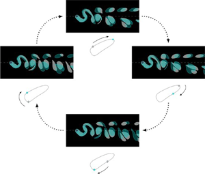
To help describe the process by which the stable and unstable P+S solutions approach each other as we move towards the ‘isola formation centre’, figure 10 illustrates the evolution of the vorticity field as we perform a clockwise loop around the P+S isola at a Reynolds number of  $Re=80 > Re_{{ {IFC}}}$ (the dashed line in figure 9a). In each of the four panels, we show in cyan the vorticity field for the parameter value identified by the square cyan symbol on the isola (shown underneath). For clarity we do not show contour levels of the vorticity but simply shade regions where the magnitude of the vorticity exceeds the threshold above which we plotted contour levels in all previous plots ( $|\omega |>0.225$). In order to indicate how the vortices move and re-orient themselves as we move around the isola, the grey shaded regions show the same regions at a previous point (identified by the grey diamond-shaped symbol) on the isola. An animation of this process is provided in the supplementary material available at https://doi.org/10.1017/jfm.2021.358.
Illustration of the evolution of the vorticity field as we move around the isola representing stable and unstable P+S solutions for  $Re=80$ (the dashed line in figure 9a). In each panel the cyan region shows the vorticity field at the point identified by the cyan square on the isola (shown underneath); the grey region shows the vorticity at the previous point, identified by the grey diamond. The shaded regions show where the magnitude of the vorticity exceeds the threshold $|\omega | > 0.225$. This is where we plotted contour levels of the vorticity in all previous plots of the vorticity field.

Figure 10(a) shows that, as discussed in § 4.3.2, an increase in amplitude along the stable P+S $^{-}$ branch (moving from A to B) causes the primary vortices to move further away from the centreline while rotating (in the anti-clockwise direction) around each other. This process leads to an increase in the asymmetry norm $\epsilon _{u}$ which at point B is close to its maximum value. As we follow the isola further along (from B to C and D; see figure 10b,c) we reach the unstable part of the solution branch along which, at larger Reynolds numbers, the flow field returned to the (now disconnected) 2S solution at the second pitchfork bifurcation. The general behaviour along this branch remains qualitatively similar to what we observed in § 4.3.2: the two primary vortices move towards the centreline and the asymmetry norm decreases, with its value at point D being close to its minimum along the isola. Finally, we return to the stable portion of the solution branch as we move along the isola from D to A, following the branch that at larger Reynolds number emanated from the first pitchfork bifurcation on the 2S solution branch. As in that case, the motion and reorientation of the primary vortices is the opposite of that observed on the downward portion of the loop: the primary vortices now move away from the centreline and rotate around each other in the opposite direction; this process is accompanied by an increase in the asymmetry norm $\epsilon _u$.
Overall, the vortices can be seen to perform an oscillatory motion as we move around the isola. As the Reynolds number decreases, the isola shrinks, causing the amplitude of this oscillatory motion to decrease and approach zero as  $Re \searrow Re_{{ {IFC}}}$, at which point the stable and unstable P+S solutions all coalesce and then spontaneously disappear. Viewed from the perspective of an increase in Reynolds number, the P+S vortex shedding mode spontaneously appears as a time-periodic solution of the Navier–Stokes equations when the Reynolds number reaches $Re_{{ {IFC}}}$. At that particular value of the Reynolds number the P+S $^{+}$ and P+S $^{-}$ solutions exist only for the specific amplitude of $A = A_{{ {IFC}}}$. For $Re > Re_{{ {IFC}}}$, four P+S solutions (two stable, two unstable) exist over a finite range of amplitudes, $A_{ {F}1}(Re) < A < A_{ {F}2}(Re)$.
5. Conclusion
We have investigated the transition from the 2S to the P+S wake mode in the two-dimensional flow past a transversely oscillating cylinder. We showed that at  $Re=100$ the transition between these wake modes arises via a spatio-temporal symmetry-breaking subcritical pitchfork bifurcation of the time-periodic 2S solution when the amplitude of the cylinder oscillation reaches a critical value, $A_{ {P}1}$. The bifurcation leads to the generation of two additional (spatio-temporal symmetry-broken) time-periodic solution branches along which the vortex shedding pattern changes from the 2S mode to the P+S pattern. Because of the subcritical character of the bifurcation, the transition between the two wake modes is hysteretic so that, following the loss of stability of the 2S solution, the flow will ‘jump’ (via a transient, non-time-periodic transition) towards the fully developed stable P+S mode. A subsequent reduction in amplitude then leads to a reverse ‘jump’ towards the 2S solution branch at a slightly lower value, $A = A_{ {F}1} < A_{ {P}1}$ where the P+S solution branch reaches a limit point. Because the P+S solution is unstable along this part of the solution branch, it cannot be observed in experiments or in direct numerical simulations based on the time-integration of the Navier–Stokes equations.
By following the solutions to larger amplitudes, we revealed the existence of a second limit point on the P+S solution branch at  $A_{ {F}2}$. The solution branch reconnects with the 2S solution branch at a second subcritical pitchfork bifurcation. This occurs at $A = A_{ {P}2} < A_{ {F}2}$, above which the 2S solution regains stability. Beyond $A=A_{ {F}2}$, the P+S solution ceases to exist. This bifurcation structure creates a second, much wider region of bistability where stable 2S and P+S solutions co-exist.
As the Reynolds number is reduced the two pitchfork bifurcations coalesce and the P+S solutions become disconnected from the now completely stable 2S solution branch. At an even smaller Reynolds number the P+S solutions disappear altogether when the isola shrinks to a point. Below this value, we obtain a single solution of 2S type.
The ‘jump’-like transitions between the stable 2S and P+S solutions explains why the two vortex shedding patterns can easily be identified in experiments or in time-dependent numerical simulations. The vorticity field evolves continuously from the 2S to P+S shedding pattern (as analysed in § 4.3), but this continuous transition occurs along unstable solution branches. Since these cannot be realised in experiments or in time-dependent numerical simulations, one can only ever observe fully developed 2S or P+S shedding patterns. However, the hysteretic nature of the transition (or conversely, the bistability of the solutions in certain parameter ranges) implies that the boundaries between these regimes are not sharp.
At  $Re=100$, the first region of bistability is so narrow that small changes to parameters (such as the channel height or the oscillation period, both of which were kept constant here) may suffice to change the criticality of the first pitchfork bifurcation from subcritical to supercritical. The transition from 2S to P+S shedding would then occur continuously, but over a very small range of amplitudes.
Motivated by the results of existing time-dependent simulations of the transition between the two vortex shedding regimes (such as those of Leontini et al. Reference Leontini, Stewart, Thompson and Hourigan2006), we restricted our analysis to solutions that are entrained by the motion of the cylinder, so that the flow field is time periodic with the same period as that of the cylinder's imposed motion. The identification of stable and unstable branches in the bifurcation diagram does therefore only assess their stability with respect to perturbations with the same period. However, we employed time-integration-based simulations to confirm that all the branches that we explicitly labelled as being stable were indeed also stable to other perturbations.
However, when performing time-dependent simulations at even larger amplitudes (specifically at values beyond the second limit point), we occasionally observed time-periodic solutions with larger periods, which are likely to have occurred via a Neimark–Sacker or torus bifurcation. In fact, it is not inconceivable that the system also has non-periodic solutions, and the phase diagram shown by Williamson & Roshko (Reference Williamson and Roshko1988) already contains regions labelled as ‘no synchronised pattern observed’ – albeit at a larger value of the Reynolds number where the vortex shedding has three-dimensional features. The computational framework developed for the current study is being extended to study the transition to such regimes.
Supplementary material
Supplementary material are available at https://doi.org/10.1017/jfm.2021.358.
Acknowledgements
We wish to acknowledge many helpful and enjoyable discussions with M. Brøns and A. Nielsen. P.M. is grateful for a PhD studentship from the Department of Mathematics at the University of Manchester.
Declaration of interests
The authors report no conflict of interest.
Appendix A. Asymmetry-control continuation
The space–time discretisation of the governing equation leads to a very large system of nonlinear algebraic equations. We solved these equations by Newton's method which requires the provision of a good initial guess for the solution. The basic approach described in § 4.1 is appropriate for computing the stable part of the 2S solution branch along which the solution for a given amplitude can be used as the initial guess for a slightly different, but nearby value. Tracing out the P+S solution branch is more complicated because the subcritical pitchfork bifurcation implies the existence of multiple solutions with the same value of the amplitude. Furthermore, following the early parts of the P+S branch actually requires a reduction in amplitude, while ensuring that the solution remains on the P+S branch, and does not jump back onto the nearby 2S solution; see figure 6. To compute these solution branches we employed a ‘displacement control’-type approach which is widely used in solid mechanics. For this purpose we augmented the residual equations arising from the space–time discretisation
 \begin{equation} \boldsymbol{r}(\boldsymbol{z};A) = \boldsymbol{0}, \end{equation}
where  $\boldsymbol {z}\in \mathbb {R}^{N}$ is the vector containing the $N$ discrete unknowns from the space–time discretisation of the Navier–Stokes equations, with the asymmetry-control equation
 \begin{equation} r_{ac}(\boldsymbol{z}) = \epsilon_{u}(\boldsymbol{z}) - \epsilon^{target}_{u} = 0, \end{equation}
where the constant  $\epsilon ^{target}_{u}$ is the prescribed (target) value of the asymmetry norm, and we treat the amplitude $A$ as an additional unknown. The solution of the $(N+1)$ equations (A1)–(A2) by Newton's method requires the repeated solution of the bordered linear systems of the form
 \begin{equation} \left( \begin{array}{cc} J & \boldsymbol{b} \\ \boldsymbol{c}^{T} & \end{array} \right) \left( \begin{array}{c} \delta \boldsymbol{z} \\ \delta A \end{array} \right) = \left( \begin{array}{c} \boldsymbol{r} \\ r_{ac} \end{array} \right). \end{equation}
Here,  $J$ is the Jacobian of the original (unbordered) system and
 \begin{equation} \boldsymbol{b} = \dfrac{\partial\boldsymbol{r}}{\partial A}, \quad \boldsymbol{c} = \dfrac{\partial r_{ac}}{\partial \boldsymbol{z}}. \end{equation}
The entries of the bordering column vector  $\boldsymbol {b}$ were computed using a finite-difference approximation and the entries of the bordering row vector $\boldsymbol {c}$ were computed analytically.
To solve the bordered system in (A3), we used GMRES, preconditioned by the block upper triangular preconditioner
 \begin{equation} P = \left( \begin{array}{c c} P_{lt} & \boldsymbol{b} \\ & \alpha \end{array} \right), \end{equation}
where  $\alpha =\boldsymbol {c}^{T}P_{lt}^{-1}\boldsymbol {b}$, which can be computed with a single application of the block lower triangular preconditioner $P_{lt}$ described in § 3. With this strategy, GMRES converged in 25–30 iterations, i.e. roughly the same number of iterations as it took to solve the unbordered system.
Appendix B. Mesh convergence tests
Figure 11 illustrates the vorticity field for a Reynolds number of 100 and an oscillation amplitude of  $A=1.2$, computed using time integration with a mesh obtained with $N_{ref}=3,\ldots ,7$ uniform spatial refinements. There are no qualitative differences in the vorticity field computed with $N_{ref}=5$, 6 and 7 uniform refinements. The results shown in this paper were therefore computed on a mesh with $N_{ref}=5$ uniform spatial refinements, corresponding to 174,622 unknowns for the time-integration-based simulations, and 16 589 090 unknowns for the space–time simulation (with $N_t=95$ time slabs).
The vorticity field in the cylinder wake, computed via time integration at  ${A=1.2}$ for successively more refined meshes; from (a) ${N_{ref}=3}$ up to (e) ${N_{ref}=7}$ uniform spatial refinements.


 Open access

