





1. Introduction
Surfactants play a pivotal role in multiphase systems by lowering interfacial tension and thereby modifying wetting and spreading behaviour. This ability underpins a wide range of applications, from enhanced oil recovery (Massarweh & Abushaikha Reference Massarweh and Abushaikha2020; Liang et al. Reference Liang, Luo, Luo, Wang, Xue and Dong2023) and coating flows, to biomedical processes (Ceresa et al. Reference Ceresa, Fracchia, Fedeli, Porta and Banat2021). Soluble surfactants are of particular interest since they partition between the bulk and the interface, dynamically altering interfacial properties and driving complex interfacial flows (Afsar-Siddiqui, Luckham & Matar Reference Afsar-Siddiqui, Luckham and Matar2003).
Equilibrium contact angle of a spreading droplet: (a) water; (b) 0.1 $\,\%$
polyethylene oxide (PEO) solution; (c) 0.03
$\,\%$
polyethylene oxide (PEO) solution; (c) 0.03 $\,\%$
polyethylene glycol (PEG) solution on a polydimethylsiloxane (PDMS) surface. The scale bar represents 0.5 mm.
$\,\%$
polyethylene glycol (PEG) solution on a polydimethylsiloxane (PDMS) surface. The scale bar represents 0.5 mm.

A robust experimental finding observed across diverse surfactant-substrate systems is that surfactants systematically reduce equilibrium contact angles: both hydrophilic and hydrophobic surfaces shift towards increased wettability (Stoebe et al. Reference Stoebe, Lin, Hill, Ward and Davis1996; Lee et al. Reference Lee, Ivanova, Starov, Hilal and Dutschk2008). Figure 1 illustrates this universal trend using our own experimental measurements of equilibrium contact angles for water, 0.1 % PEO solution and 0.03 % PEG solution on a PDMS substrate, where we observe a clear reduction in contact angle upon surfactant addition. Even though they are not classical surfactants with hydrophobic tails, they are surface active and reduce the interfacial tension by adsorbing on the interface. Experimental results of spreading of droplets upon addition of classical surfactants line Triton X-100 and Poloxamer are shown in Appendix A. Beyond this universal trend, surfactants can also produce counterintuitive behaviours such as autophobing, where droplets spontaneously recoil upon surfactant addition (Bera et al. Reference Bera, Duits, Stuart, Van Den Ende and Mugele2016; Tadmor et al. Reference Tadmor, Baksi, Gulec, Jadhav, N’guessan, Sen, Somasi, Tadmor, Wasnik and Yadav2019). These phenomena point to a mechanism beyond simple interfacial tension reduction: wall adsorption must play a central role.
Over the last two decades, several numerical frameworks have been developed to model soluble surfactants in multiphase flows. Xu, Shi & Lai (Reference Xu, Shi and Lai2018) introduced a level-set formulation for soluble surfactants, Khatri & Tornberg (Reference Khatri and Tornberg2014) developed an interface-tracking approach, while diffuse-interface methods were pursued by Teigen et al. (Reference Teigen, Song, Lowengrub and Voigt2011), Engblom et al. (Reference Engblom, Do-Quang, Amberg and Tornberg2013). Building on these, Zhu et al. (Reference Zhu, Kou, Yao, Wu, Yao and Sun2019) extended a phase-field method to include soluble surfactants in moving contact line problems. Phase-field models, particularly those based on the Cahn–Hilliard formulation, have become increasingly popular due to their thermodynamic consistency and their ability to regularize the singular stresses at the contact line (Jacqmin Reference Jacqmin2000; Yue Reference Yue2020; Qiu et al. Reference Qiu, Cueto-Felgueroso, Pahlavan, Primkulov and Juanes2025). Yet despite their sophistication, all existing formulations on solid substrates share a common limitation.
All formulations on solid substrates neglect surfactant adsorption at walls. Without wall adsorption, surfactants only reduce fluid–fluid interfacial tension $\sigma$
, rescaling Young’s equation as
$\sigma$
, rescaling Young’s equation as $\sigma \cos \theta = \sigma _0 \cos \theta _0$
, where
$\sigma \cos \theta = \sigma _0 \cos \theta _0$
, where $\theta _0$
is the equilibrium angle for the clean system and
$\theta _0$
is the equilibrium angle for the clean system and $\theta$
is the equilibrium angle of the contaminated system. This rescaling amplifies the substrate’s wetting character – hydrophilic substrates become more hydrophilic, hydrophobic substrates more hydrophobic – but cannot produce the universal shift towards hydrophilicity observed experimentally. Neither can it explain autophobing, which requires asymmetric modification of the solid–liquid and solid–gas interfacial tensions. This fundamental mismatch between model predictions and experimental observations reveals that a critical mechanism is missing.
$\theta$
is the equilibrium angle of the contaminated system. This rescaling amplifies the substrate’s wetting character – hydrophilic substrates become more hydrophilic, hydrophobic substrates more hydrophobic – but cannot produce the universal shift towards hydrophilicity observed experimentally. Neither can it explain autophobing, which requires asymmetric modification of the solid–liquid and solid–gas interfacial tensions. This fundamental mismatch between model predictions and experimental observations reveals that a critical mechanism is missing.
In this work, we provide the missing mechanism, i.e. solid adsorption by developing a thermodynamically consistent phase-field model that incorporates surfactant adsorption on solid walls in addition to interfacial adsorption. We demonstrate that this single addition – solid surface adsorption – resolves the qualitative discrepancy between prior numerical predictions and experiments: our model predicts a universal shift towards hydrophilicity across all contact angles (Staniscia, Guzman & Kanduc Reference Staniscia, Guzman and Kanduc2022), consistent with experimental trends.
We validate the model against clean-droplet spreading benchmarks, derive scaling laws for the solid adsorption layer and compare predictions with experimental measurements of polymeric surfactants, including autophobing phenomena. We further illustrate the role of wall adsorption in Couette flow, where we find that only preferential adsorption on the solid–liquid interface enhances droplet stability under shear, extending the critical capillary number by 20 %–30 %.
This paper is organized as follows. In § 2 we introduce the phase-field framework: the bulk free energy and the resulting Cahn–Hilliard Navier–Stokes equations (§ 2.2). The wall free energy is formulated in § 2.3, resulting in kinetic boundary conditions for surfactant transport and contact line movement. Equilibrium properties are analysed at the fluid–fluid interface (§ 2.5) and for the solid-adsorption layer (§ 2.6). The numerical scheme is described in § 3 and the experimental methods are given in Appendix E. Results are presented in § 4, progressing from validation through spreading dynamics, scaling law verification and Couette flow stability. Conclusions are summarized in § 5.
2. Phase-field method
We consider an incompressible two-phase system with $\phi$
being the phase field variable ranging from –1 in fluid 1, to +1 in fluid 2 via a diffuse interface of thickness
$\phi$
being the phase field variable ranging from –1 in fluid 1, to +1 in fluid 2 via a diffuse interface of thickness $\epsilon$
as shown in figure 2. The free energy is a combination of three energies excluding the kinetic energy, namely the mixing energy, the energy due to the presence of surfactants and the surface energy. We will discuss the surface energy extensively in § 2.3.
$\epsilon$
as shown in figure 2. The free energy is a combination of three energies excluding the kinetic energy, namely the mixing energy, the energy due to the presence of surfactants and the surface energy. We will discuss the surface energy extensively in § 2.3.
Illustration of a surfactant-laden fluid–fluid system on a solid substrate.

2.1. Free energy of the bulk
The mixing energy per unit volume (Cahn & Hilliard Reference Cahn and Hilliard1958) can be written as
 \begin{equation} F_m(\phi , \boldsymbol{\nabla }\phi)=\lambda \left ( \frac {1}{2}|\boldsymbol{\nabla }\phi |^2 + F_0(\phi)\right) \!, \end{equation}
where
 \begin{equation} F_0(\phi )=\frac {(\phi ^2-1)^2}{4\epsilon ^2} \end{equation}
is the double-well potential with minima in the bulk phases (–1 and +1) thereby preferring the separation of the system into two phases. The square gradient term of the mixing energy $\lambda |\boldsymbol{\nabla }\phi |^2 /2$
on the other hand prefers complete mixing of the two phases. Here
$\lambda |\boldsymbol{\nabla }\phi |^2 /2$
on the other hand prefers complete mixing of the two phases. Here $\lambda$
is the mixing energy density often defined as
$\lambda$
is the mixing energy density often defined as
 \begin{equation} \lambda = \frac {3}{2\sqrt {2}}\sigma \epsilon, \end{equation}
where $\sigma$
is the interfacial tension between the two fluids.
$\sigma$
is the interfacial tension between the two fluids.
In the presence of surfactants, additional energetic contributions arise from spatial inhomogeneity and bulk mixing entropy. Following Engblom et al. (Reference Engblom, Do-Quang, Amberg and Tornberg2013), we adopt a logarithmic free-energy density per unit volume,
 \begin{equation} F_{\psi }(\psi ,\boldsymbol{\nabla }\psi ) = \frac {\lambda }{\epsilon ^{2}}\,{\textit{Pi}}\, \big [\,\psi \ln \psi + (1-\psi )\ln (1-\psi )\,\big ] \;+\; \frac {\lambda _{s}}{2}\,|\boldsymbol{\nabla }\psi |^{2}, \end{equation}
where $\psi \in [0,1]$
is the local surfactant concentration, Pi is a temperature-dependent energetic scale tied to the diffusive entropy of the mixture (Engblom et al. Reference Engblom, Do-Quang, Amberg and Tornberg2013) and
$\psi \in [0,1]$
is the local surfactant concentration, Pi is a temperature-dependent energetic scale tied to the diffusive entropy of the mixture (Engblom et al. Reference Engblom, Do-Quang, Amberg and Tornberg2013) and $\lambda _s\gt 0$
is a gradient-penalty coefficient.
$\lambda _s\gt 0$
is a gradient-penalty coefficient.
The logarithmic term encodes the entropy of mixing of surfactant and solvent: it is strictly convex on $(0,1)$
, discourages unphysical saturation (
$(0,1)$
, discourages unphysical saturation ( $\psi \to 0$
or
$\psi \to 0$
or $1$
), and guarantees a thermodynamically consistent chemical potential. The gradient term
$1$
), and guarantees a thermodynamically consistent chemical potential. The gradient term $\lambda _s|\boldsymbol{\nabla }\psi |^{2}$
regularizes sharp concentration fronts by penalizing steep gradients; physically it sets a finite adsorption-layer thickness and mathematically it ensures well-posedness of the coupled transport by contributing a
$\lambda _s|\boldsymbol{\nabla }\psi |^{2}$
regularizes sharp concentration fronts by penalizing steep gradients; physically it sets a finite adsorption-layer thickness and mathematically it ensures well-posedness of the coupled transport by contributing a $-\lambda _s{\nabla} ^2\psi$
term to the chemical potential. We return to the far-from-wall equilibrium profile implied by (2.4) in § 2.5. Critically, its presence also provides the mathematical structure necessary for the surface adsorption boundary condition derived in § 2.4, representing a key difference from prior work (Zhu et al. Reference Zhu, Kou, Yao, Wu, Yao and Sun2019).
$-\lambda _s{\nabla} ^2\psi$
term to the chemical potential. We return to the far-from-wall equilibrium profile implied by (2.4) in § 2.5. Critically, its presence also provides the mathematical structure necessary for the surface adsorption boundary condition derived in § 2.4, representing a key difference from prior work (Zhu et al. Reference Zhu, Kou, Yao, Wu, Yao and Sun2019).
The decrease of free energy per unit volume due to adsorption of surfactants onto the interface is governed by $F_1$
given as
$F_1$
given as
 \begin{equation} F_{1}(\phi ,\psi )= -\frac {\lambda }{4\epsilon ^2} \psi (1-\phi ^2)^2\;. \end{equation}
Finally, complementary to $F_1$
, the free surfactants in the bulk are penalized by an increase in free energy per unit volume,
$F_1$
, the free surfactants in the bulk are penalized by an increase in free energy per unit volume, $F_{\textit{Ex}}$
, given as
$F_{\textit{Ex}}$
, given as
 \begin{equation} F_{\textit{Ex}}(\phi ,\psi )= \frac {\lambda }{2 \textit{Ex}\epsilon ^2} \psi \phi ^2 \;, \end{equation}
where ${Ex}$
is the constant related to how soluble the phases are with each other. Therefore, the total bulk free energy in the presence of surfactants can be given as
${Ex}$
is the constant related to how soluble the phases are with each other. Therefore, the total bulk free energy in the presence of surfactants can be given as
 \begin{equation} F_{\textit{bulk}}(\phi ,\psi ,\boldsymbol{\nabla }\phi ,\boldsymbol{\nabla }\psi )= F_m(\phi , \boldsymbol{\nabla }\phi )+F_{\psi }(\psi ,\boldsymbol{\nabla }\psi )+F_{1}(\phi ,\psi )+F_{\textit{Ex}}(\phi ,\psi ) \;. \end{equation}
2.2. Cahn–Hilliard Navier–Stokes governing equations
From the bulk free energy defined in § 2.1, we derive transport equations for the phase field variable $\phi$
and surfactant concentration
$\phi$
and surfactant concentration $\psi$
using variational principles. The complete derivation is provided in Appendix B; here we summarize the results.
$\psi$
using variational principles. The complete derivation is provided in Appendix B; here we summarize the results.
2.2.1. Navier–Stokes equations
The incompressible Navier–Stokes equations coupled to the phase-field variables are
 \begin{equation} \rho\! \left (\frac {\partial \boldsymbol{u}}{\partial t} + \boldsymbol{u}\boldsymbol{\cdot }\boldsymbol{\nabla }\boldsymbol{u}\right ) + \boldsymbol{J}.\boldsymbol{\nabla }\boldsymbol{u} = -\boldsymbol{\nabla }\!p + \boldsymbol{\nabla }\boldsymbol{\cdot }\left (\mu \left (\boldsymbol{\nabla }\boldsymbol{u} + \boldsymbol{\nabla }\boldsymbol{u}^{\mathrm{T}}\right )\right ) + G_\phi \boldsymbol{\nabla }\phi + G_\psi \boldsymbol{\nabla }\psi , \end{equation}
 \begin{equation} \boldsymbol{\nabla }\boldsymbol{\cdot }\boldsymbol{u} = 0, \end{equation}
where $\rho$
and
$\rho$
and $\mu$
are density and viscosity interpolated between the two fluids,
$\mu$
are density and viscosity interpolated between the two fluids,
 \begin{equation} \rho =\rho _1\frac { (1+\phi )}{2} + \rho _2\frac { (1-\phi )}{2}, \end{equation}
 \begin{equation} \mu =\mu _1\frac { (1+\phi )}{2} + \mu _2\frac { (1-\phi )}{2}. \end{equation}
Here $\boldsymbol{J}$
is the diffusive flux caused by deviation of
$\boldsymbol{J}$
is the diffusive flux caused by deviation of $u$
from mass-averaged velocities (Abels, Garcke & Grün Reference Abels, Garcke and Grün2012; Zhu et al. Reference Zhu, Kou, Yao, Wu, Yao and Sun2019) and is expanded to be
$u$
from mass-averaged velocities (Abels, Garcke & Grün Reference Abels, Garcke and Grün2012; Zhu et al. Reference Zhu, Kou, Yao, Wu, Yao and Sun2019) and is expanded to be
 \begin{equation} \boldsymbol{J} = \frac {\rho _1-\rho _2}{2}M_\phi \boldsymbol{\nabla }G_\phi . \end{equation}
The terms $G_\phi \boldsymbol{\nabla }\phi$
and
$G_\phi \boldsymbol{\nabla }\phi$
and $G_\psi \boldsymbol{\nabla }\psi$
represent surface tension forces acting at the interfaces and
$G_\psi \boldsymbol{\nabla }\psi$
represent surface tension forces acting at the interfaces and $M_\phi$
is the phase-field mobility.
$M_\phi$
is the phase-field mobility.
2.2.2. Cahn–Hilliard equation for the phase field
The phase field variable $\phi$
(conserved) evolves via
$\phi$
(conserved) evolves via
 \begin{equation} \frac {\mathrm{D} \phi }{\mathrm{D} t} = M_\phi {\nabla} ^2 G_\phi , \end{equation}
where $G_\phi$
is the chemical potential of the phase field variable:
$G_\phi$
is the chemical potential of the phase field variable:
 \begin{equation} G_\phi =\lambda \left (F_0'(\phi ) - {\nabla} ^2 \phi + \frac {\psi \phi }{{Ex}\epsilon ^2} + \frac {\psi \phi (1-\phi ^2)}{\epsilon ^2} \right )\!. \end{equation}
Here, $F_0'(\phi ) = (\phi ^3 - \phi )/\epsilon ^2$
is the derivative of the double-well potential. The last two terms arise from variational derivatives of the interfacial adsorption energy
$F_0'(\phi ) = (\phi ^3 - \phi )/\epsilon ^2$
is the derivative of the double-well potential. The last two terms arise from variational derivatives of the interfacial adsorption energy $F_1$
and bulk surfactant penalty
$F_1$
and bulk surfactant penalty $F_{\textit{Ex}}$
(see Appendix B).
$F_{\textit{Ex}}$
(see Appendix B).
2.2.3. Cahn–Hilliard equation for surfactant
The surfactant concentration $\psi$
(conserved) evolves via
$\psi$
(conserved) evolves via
 \begin{equation} \frac {\mathrm{D} \psi }{\mathrm{D} t} = \boldsymbol{\nabla }\boldsymbol{\cdot }(M_\psi \boldsymbol{\nabla }G_\psi ), \end{equation}
where $M_\psi = m_\psi \psi (1-\psi )$
is a degenerate mobility that prevents unphysical surfactant concentrations exceeding saturation: the mobility vanishes as
$M_\psi = m_\psi \psi (1-\psi )$
is a degenerate mobility that prevents unphysical surfactant concentrations exceeding saturation: the mobility vanishes as $\psi \to 0$
or
$\psi \to 0$
or $\psi \to 1$
, enforcing physical bounds on the concentration field. Also,
$\psi \to 1$
, enforcing physical bounds on the concentration field. Also, $G_\psi$
is the chemical potential of the surfactant concentration:
$G_\psi$
is the chemical potential of the surfactant concentration:
 \begin{equation} G_\psi = \frac {\lambda }{\epsilon ^2}\left ({\textit{Pi}} \ln \left (\frac {\psi }{1-\psi }\right ) + \frac {\phi ^2}{2{Ex}} - \frac {(1-\phi ^2)^2}{4}\right ) - \lambda _s {\nabla} ^2 \psi . \end{equation}
The logarithmic term encodes thermodynamic consistency (entropy of mixing), the $\phi$
-dependent terms couple surfactant to interfacial position and the
$\phi$
-dependent terms couple surfactant to interfacial position and the $-\lambda _s{\nabla} ^2\psi$
term regularizes sharp concentration gradients. This final term is crucial: it introduces a characteristic length scale and necessitates an additional boundary condition at walls (discussed in § 2.4).
$-\lambda _s{\nabla} ^2\psi$
term regularizes sharp concentration gradients. This final term is crucial: it introduces a characteristic length scale and necessitates an additional boundary condition at walls (discussed in § 2.4).
2.3. Surface energy
When the diffuse interface intersects a solid surface, contact lines emerge that require special treatment. The thermodynamic treatment of the wall requires a free energy functional that correctly captures the equilibrium contact angle and provides kinetic boundary conditions for dynamic wetting.
For a clean two-phase system without surfactants, the wall free energy per unit area follows the standard form (Yue & Feng Reference Yue and Feng2011),
 \begin{equation} f_w = -\sigma _0 \cos \theta _{S,0} g(\phi ) + \frac {\sigma _{w1,0} + \sigma _{w2,0}}{2}, \end{equation}
where $\sigma _{w1,0}$
and
$\sigma _{w1,0}$
and $\sigma _{w2,0}$
are the clean surface tensions between the solid and fluids 1 and 2, respectively, and
$\sigma _{w2,0}$
are the clean surface tensions between the solid and fluids 1 and 2, respectively, and $g(\phi )$
is a switch function that modulates the wall energy smoothly across the diffuse interface. The switch function must satisfy
$g(\phi )$
is a switch function that modulates the wall energy smoothly across the diffuse interface. The switch function must satisfy $g(\pm 1) = \pm 0.5$
so that in pure bulk phases,
$g(\pm 1) = \pm 0.5$
so that in pure bulk phases, $f_w$
recovers the respective solid–fluid interfacial tensions.
$f_w$
recovers the respective solid–fluid interfacial tensions.
This construction is consistent with Young’s equation:
 \begin{equation} \sigma _0 \cos \theta _{S,0} = \sigma _{w1,0} - \sigma _{w2,0}. \end{equation}
In the presence of surfactants, both fluid–fluid and solid–fluid surface tensions are modified. Therefore, the switch function $g(\phi )$
must be generalized to account for surfactant-induced changes in interfacial energetics.
$g(\phi )$
must be generalized to account for surfactant-induced changes in interfacial energetics.
To incorporate the surfactant effects we follow Yue (Reference Yue2020), and derive $g(\phi )$
to be
$g(\phi )$
to be
 \begin{equation} g(\phi ) = \frac {3}{2\sqrt {2}}\sqrt {A} \left [\phi + \frac {B}{6A}\phi ^3 + \frac {C}{10A}\phi ^5 + \frac {D}{14A}\phi ^7\right ]\!, \end{equation}
where
 \begin{align} A &= \frac {1}{2} + \frac {\psi _b}{2} - \frac {\psi _b}{E_x} - \psi _b, \\[-12pt]\nonumber \end{align}
 \begin{align} B &= -1 + \frac {\psi _b}{E_x} + \psi _b, \\[-12pt]\nonumber \end{align}
 \begin{align} C &= \frac {1}{2} - \frac {\psi _b}{2}, \\[-12pt]\nonumber \end{align}
 \begin{align} D &= 14A\left [\frac {\sqrt {2}}{3\sqrt {A}} - 1 - \frac {B}{6A} - \frac {C}{10A}\right ]\!. \end{align}
The derivation of this modified switch function is given in Appendix C. When $\psi _b \to 0$
(no surfactant), this reduces to the clean case
$\psi _b \to 0$
(no surfactant), this reduces to the clean case $g(\phi ) = \phi (3-\phi ^2)/4$
. The surfactant-dependent terms modify the switch function to reflect changes in interfacial energetics induced by adsorption.
$g(\phi ) = \phi (3-\phi ^2)/4$
. The surfactant-dependent terms modify the switch function to reflect changes in interfacial energetics induced by adsorption.
2.3.1. Surface adsorption
When surfactants are added to a two-phase system in contact with a solid, they could adsorb on the solid–fluid interfaces, thereby reducing the wall–fluid interfacial tensions (Haidara, Chaudhury & Owen Reference Haidara, Chaudhury and Owen1995).
We model the reduction in solid–fluid surface tension using the Langmuir–Szyszkowski equation of state (Soligo, Roccon & Soldati Reference Soligo, Roccon and Soldati2019),
 \begin{equation} \sigma _{wf} = \sigma _{wf,0}[1 + \beta \log (1-\psi )], \end{equation}
where $\sigma _{wf,0}$
is the clean wall–fluid surface tension,
$\sigma _{wf,0}$
is the clean wall–fluid surface tension, $\beta$
is the elasticity number (
$\beta$
is the elasticity number ( $0 \lt \beta \lt 1$
) controlling surfactant strength and
$0 \lt \beta \lt 1$
) controlling surfactant strength and $\psi$
is the local surfactant concentration at the wall. This logarithmic form, also known as the Szyszkowski equation, is thermodynamically equivalent to the Langmuir adsorption isotherm. The logarithmic dependence emerges from the Gibbs adsorption equation relating surface tension to surface excess concentration.
$\psi$
is the local surfactant concentration at the wall. This logarithmic form, also known as the Szyszkowski equation, is thermodynamically equivalent to the Langmuir adsorption isotherm. The logarithmic dependence emerges from the Gibbs adsorption equation relating surface tension to surface excess concentration.
The Langmuir–Szyszkowski equation is chosen for its thermodynamic consistency and widespread validation for common surfactants at moderate concentrations. This isotherm assumes monolayer adsorption with equivalent, non-interacting adsorption sites. Alternative isotherms can be incorporated into the present framework by replacing (2.21) with the appropriate equation of state. For dilute surfactant concentrations ( $\psi \ll 1$
), a linear equation of state
$\psi \ll 1$
), a linear equation of state $\sigma _{wf} = \sigma _{wf,0}(1 - \beta \psi )$
provides a simpler approximation that is often sufficient. For systems with lateral interactions between adsorbed molecules, the Frumkin isotherm offers a more accurate description, while the Freundlich isotherm is appropriate for heterogeneous surfaces with a distribution of adsorption energies. However, the Langmuir–Szyszkowski form suffices for the phenomena investigated here and we proceed with that.
$\sigma _{wf} = \sigma _{wf,0}(1 - \beta \psi )$
provides a simpler approximation that is often sufficient. For systems with lateral interactions between adsorbed molecules, the Frumkin isotherm offers a more accurate description, while the Freundlich isotherm is appropriate for heterogeneous surfaces with a distribution of adsorption energies. However, the Langmuir–Szyszkowski form suffices for the phenomena investigated here and we proceed with that.
Incorporating surfactant adsorption on both solid–fluid interfaces into Young’s equation gives
 \begin{equation} \sigma \cos \theta _S = \sigma _0 \cos \theta _{S,0} + \sigma _{w1,0}\beta _{s1}\log (1-\psi ) - \sigma _{w2,0}\beta _{s2}\log (1-\psi ), \end{equation}
where $\beta _{s1}$
and
$\beta _{s1}$
and $\beta _{s2}$
are the surfactant strengths on the solid-phase 1 and solid-phase 2 interfaces, respectively. Different elasticity numbers allow for asymmetric adsorption behaviour on the two interfaces. This asymmetry is crucial for phenomena like autophobing, where differential adsorption on solid–liquid versus solid–gas interfaces can cause droplet recession.
$\beta _{s2}$
are the surfactant strengths on the solid-phase 1 and solid-phase 2 interfaces, respectively. Different elasticity numbers allow for asymmetric adsorption behaviour on the two interfaces. This asymmetry is crucial for phenomena like autophobing, where differential adsorption on solid–liquid versus solid–gas interfaces can cause droplet recession.
The complete wall energy per unit area becomes
 \begin{equation} \begin{aligned} f_w = -\left [\sigma _0 \cos \theta _{S0} + \log (1-\psi )(\sigma _{w1,0}\beta _{s1} - \sigma _{w2,0}\beta _{s2})\right ] g(\phi ) \\[3pt] + \log (1-\psi )\frac {\sigma _{w1,0}\beta _{s1} +\sigma _{w2,0}\beta _{s2}}{2} + \frac {\sigma _{w1,0} +\sigma _{w2,0}}{2}\;. \end{aligned} \end{equation}
This expression contains three physically distinct contributions: (i) surfactant-modified Young stress modulated by the switch function $g(\phi )$
, (ii) average reduction in wall–fluid tensions independent of
$g(\phi )$
, (ii) average reduction in wall–fluid tensions independent of $\phi$
and (iii) baseline wall energy for the clean system.
$\phi$
and (iii) baseline wall energy for the clean system.
Experimental studies indicate that surfactant-induced reduction of wall–fluid surface tension saturates at high coverage and does not decrease indefinitely (Chang & Franses Reference Chang and Franses1995; Ju et al. Reference Ju, Jiang, Geng, Wang and Zhang2017; López-Díaz et al. Reference López-Díaz, García-Mateos and Velázquez2006; Soligo et al. Reference Soligo, Roccon and Soldati2019). To prevent unphysical values, we limit the minimum surface tension to half the clean-wall value,
 \begin{equation} \sigma _{w\alpha }(\psi ) = \sigma _{w\alpha ,0} \max [0.5, 1 + \beta _{s\alpha }\log (1-\psi )], \end{equation}
for each wall–fluid interface $\alpha \in \{1,2\}$
.
$\alpha \in \{1,2\}$
.
Soligo et al. (Reference Soligo, Roccon and Soldati2019) note that ‘according to experimental observations, surface tension does not decrease below this threshold (roughly)’. The factor 0.5 provides a physically reasonable bound ensuring $\sigma _{w\alpha } \geqslant 0$
and a smooth transition from the logarithmic regime to a saturated plateau at high
$\sigma _{w\alpha } \geqslant 0$
and a smooth transition from the logarithmic regime to a saturated plateau at high $\psi$
.
$\psi$
.
With the wall free energy fully specified, we now derive the corresponding boundary conditions for the phase field and surfactant concentration in § 2.4.
2.4. Cahn–Hilliard Navier–Stokes boundary conditions
We now collect all the surface integral terms from the variational derivative of the bulk free energy with respect to $\phi$
, and add it into the variational derivative of the surface energy term with respect to
$\phi$
, and add it into the variational derivative of the surface energy term with respect to $\phi$
, to get
$\phi$
, to get
 \begin{equation} \delta F = \lambda \oint (\boldsymbol{\nabla }\phi \boldsymbol{\cdot} \boldsymbol{n} )\delta \phi )){\rm d}S + \oint f'w(\phi )\delta \phi {\rm d}S. \end{equation}
Requiring that the wall contribution to $\mathrm{d}F/\mathrm{d}t$
be non-positive (thermodynamic dissipation), the relaxation boundary condition for
$\mathrm{d}F/\mathrm{d}t$
be non-positive (thermodynamic dissipation), the relaxation boundary condition for $\phi$
takes the form
$\phi$
takes the form
 \begin{equation} \frac {\partial \phi }{\partial t} + \boldsymbol{u}\boldsymbol{\cdot }\boldsymbol{\nabla }\phi = -\varGamma L_\phi , \end{equation}
where $L_{\phi }$
is the wall potential (as introduced earlier) of the phase field variable and is expressed as
$L_{\phi }$
is the wall potential (as introduced earlier) of the phase field variable and is expressed as
 \begin{equation} L_{\phi }=\lambda \boldsymbol{n} \boldsymbol{\cdot }\boldsymbol{\nabla }\phi + \frac {\partial f_w(\phi ,\psi )}{\partial \phi } , \end{equation}
where the capping from (2.24) introduces piecewise behaviour in the derivatives $\partial f_w/\partial \phi$
. Defining
$\partial f_w/\partial \phi$
. Defining
 \begin{equation} S_1 = 1 + \beta _{s1}\log (1-\psi ), \quad S_2 = 1 + \beta _{s2}\log (1-\psi ), \end{equation}
the derivative with respect to $\phi$
becomes (with
$\phi$
becomes (with $K = \sigma _0\cos \theta _{S,0}$
)
$K = \sigma _0\cos \theta _{S,0}$
)
 \begin{equation} \frac {\partial f_w}{\partial \phi }(\psi ,\phi ) = g'(\phi ) \times \begin{cases} \frac {K}{2}, & \text{if } S_1, S_2 \leqslant 0.5,\\[5pt] K - \sigma _{w1}\beta _{s1}\log (1-\psi ) - \frac {\sigma _{w2}}{2}, & \text{if } S_1 \leqslant 0.5 \lt S_2,\\[9pt] K + \sigma _{w2}\beta _{s2}\log (1-\psi ) + \frac {\sigma _{w1}}{2}, & \text{if } S_2 \leqslant 0.5 \lt S_1,\\[9pt] K + (\sigma _{w2}\beta _{s2} - \sigma _{w1}\beta _{s1})\log (1-\psi ), & \text{if } S_1, S_2 \gt 0.5, \end{cases} \end{equation}
and $g'(\phi )$
can be found in (C6). This governs the behaviour of the contact line on the surface.
$g'(\phi )$
can be found in (C6). This governs the behaviour of the contact line on the surface. $\varGamma = 1/\mu _f \epsilon$
in (2.26) is a positive phenomenological parameter that controls how fast the contact line relaxes to the equilibrium angle
$\varGamma = 1/\mu _f \epsilon$
in (2.26) is a positive phenomenological parameter that controls how fast the contact line relaxes to the equilibrium angle $\theta _S$
. The variable
$\theta _S$
. The variable $\mu _f$
is known as the contact line friction. This boundary condition governs the dynamics of the contact line according to the contact angle.
$\mu _f$
is known as the contact line friction. This boundary condition governs the dynamics of the contact line according to the contact angle.
Similarly, including the surface integral terms from the variational derivative of the free energy with respect to $\psi$
, into the variational derivative of the surface energy term with respect to
$\psi$
, into the variational derivative of the surface energy term with respect to $\psi$
, we get
$\psi$
, we get
 \begin{equation} \delta F = \lambda _s\oint (\boldsymbol{\nabla }\psi .\boldsymbol{n} )\delta \psi )){\rm d}S + \oint f'w(\psi )\delta \psi {\rm d}S. \end{equation}
Similarly, requiring dissipation of the surface free energy contribution, the relaxation boundary condition for $\psi$
takes the form
$\psi$
takes the form
 \begin{equation} \frac {\partial \psi }{\partial t} + \boldsymbol{u}\boldsymbol{\cdot }\boldsymbol{\nabla }\psi = -\varGamma _s L_\psi , \end{equation}
where $\varGamma _s$
is a positive constant determining how fast surfactant adsorbs on the walls and
$\varGamma _s$
is a positive constant determining how fast surfactant adsorbs on the walls and $L_{\psi }$
is the wall potential of the surfactant concentration variable and is expressed as
$L_{\psi }$
is the wall potential of the surfactant concentration variable and is expressed as
 \begin{equation} L_{\psi }=\lambda _s \boldsymbol{n} \boldsymbol{\cdot }\boldsymbol{\nabla }\psi + \frac {\partial f_w(\phi ,\psi )}{\partial \psi } , \end{equation}
where the capping introduces piecewise behaviour in the derivative $\partial f_w/\partial \psi$
. Defining
$\partial f_w/\partial \psi$
. Defining
 \begin{equation} S_1 = 1 + \beta _{s1}\log (1-\psi ), \quad S_2 = 1 + \beta _{s2}\log (1-\psi ), \end{equation}
the derivative with respect to $\psi$
is
$\psi$
is
 \begin{align} \frac {\partial f_w}{\partial \psi }(\phi ,\psi ) = \frac {1}{1-\psi } \times \begin{cases} 0, & \text{if } S_1, S_2 \leqslant 0.5,\\[9pt] -\sigma _{w1}\beta _{s1}\left [g(\phi ) + \frac {1}{2}\right ]\!, & \text{if } S_1 \leqslant 0.5 \lt S_2,\\[11pt] \sigma _{w2}\beta _{s2}\left [g(\phi ) - \frac {1}{2}\right ]\!, & \text{if } S_2 \leqslant 0.5 \lt S_1,\\[9pt] (\sigma _{w2}\beta _{s2} - \sigma _{w1}\beta _{s1})g(\phi ) - \frac {\sigma _{w2}\beta _{s2} + \sigma _{w1}\beta _{s1}}{2}, & \text{if } S_1, S_2 \gt 0.5. \end{cases} \end{align}
When both interfaces saturate ( $S_1, S_2 \leqslant 0.5$
), the wall becomes ‘surfactant-insensitive’ and
$S_1, S_2 \leqslant 0.5$
), the wall becomes ‘surfactant-insensitive’ and $\partial f_w/\partial \psi = 0$
. These piecewise expressions recover the uncapped forms when
$\partial f_w/\partial \psi = 0$
. These piecewise expressions recover the uncapped forms when $S_1, S_2 \gt 0.5$
, ensuring thermodynamic consistency while preventing unphysical behaviour at high surfactant coverage.
$S_1, S_2 \gt 0.5$
, ensuring thermodynamic consistency while preventing unphysical behaviour at high surfactant coverage.
Finally, we have $\boldsymbol{n}\boldsymbol{\cdot }\boldsymbol{\nabla }\phi = 0$
,
$\boldsymbol{n}\boldsymbol{\cdot }\boldsymbol{\nabla }\phi = 0$
, $\boldsymbol{n}\boldsymbol{\cdot }\boldsymbol{\nabla }G_\phi = 0$
,
$\boldsymbol{n}\boldsymbol{\cdot }\boldsymbol{\nabla }G_\phi = 0$
, $\boldsymbol{n}\boldsymbol{\cdot }\boldsymbol{\nabla }G_\psi = 0$
and
$\boldsymbol{n}\boldsymbol{\cdot }\boldsymbol{\nabla }G_\psi = 0$
and $\boldsymbol{u} = \boldsymbol{u}_w$
, which are the no flux across walls for
$\boldsymbol{u} = \boldsymbol{u}_w$
, which are the no flux across walls for $\phi$
, no flux of chemical potential across walls for
$\phi$
, no flux of chemical potential across walls for $\phi$
and
$\phi$
and $\psi$
variables and no slip boundary condition, respectively.
$\psi$
variables and no slip boundary condition, respectively.
The gradient penalty term $({\lambda _s}/{2})|\boldsymbol{\nabla }\psi |^2$
introduced in
$({\lambda _s}/{2})|\boldsymbol{\nabla }\psi |^2$
introduced in $\S$
2.1 is structurally critical to the model, not merely a regularization term. Its variational derivative contributes a
$\S$
2.1 is structurally critical to the model, not merely a regularization term. Its variational derivative contributes a $-\lambda _s{\nabla} ^2\psi$
term to the surfactant chemical potential
$-\lambda _s{\nabla} ^2\psi$
term to the surfactant chemical potential $G_\psi$
(2.16), which is the only term in
$G_\psi$
(2.16), which is the only term in $G_\psi$
that carries spatial information about
$G_\psi$
that carries spatial information about $\psi$
itself; without it,
$\psi$
itself; without it, $G_\psi$
reduces to a purely local algebraic function of
$G_\psi$
reduces to a purely local algebraic function of $\psi$
and
$\psi$
and $\phi$
, with no coupling between neighbouring values of the concentration field. More importantly, the surface integral arising from the variational derivative of
$\phi$
, with no coupling between neighbouring values of the concentration field. More importantly, the surface integral arising from the variational derivative of $F_\psi$
with respect to
$F_\psi$
with respect to $\psi$
produces the
$\psi$
produces the $\lambda _s\boldsymbol{n}\boldsymbol{\cdot }\boldsymbol{\nabla }\psi$
term in the wall potential
$\lambda _s\boldsymbol{n}\boldsymbol{\cdot }\boldsymbol{\nabla }\psi$
term in the wall potential $L_\psi$
(2.32), which is the mechanism by which the wall affinity
$L_\psi$
(2.32), which is the mechanism by which the wall affinity $\beta _s$
prescribes a non-trivial normal gradient of
$\beta _s$
prescribes a non-trivial normal gradient of $\psi$
at the boundary. In the absence of the
$\psi$
at the boundary. In the absence of the $|\boldsymbol{\nabla }\psi |^2$
term, both contributions vanish simultaneously: the boundary condition collapses to the purely algebraic condition
$|\boldsymbol{\nabla }\psi |^2$
term, both contributions vanish simultaneously: the boundary condition collapses to the purely algebraic condition $\partial f_w/\partial \psi = 0$
, which imposes no flux, and the Cahn–Hilliard equation for
$\partial f_w/\partial \psi = 0$
, which imposes no flux, and the Cahn–Hilliard equation for $\psi$
becomes second order in space, requiring only the no-flux condition on
$\psi$
becomes second order in space, requiring only the no-flux condition on $G_\psi$
already satisfied at the wall. The wall energy can influence the contact line through
$G_\psi$
already satisfied at the wall. The wall energy can influence the contact line through $f_w$
, but has no mathematical pathway to alter the bulk surfactant distribution. The
$f_w$
, but has no mathematical pathway to alter the bulk surfactant distribution. The $|\boldsymbol{\nabla }\psi |^2$
term is therefore what promotes the surfactant equation to fourth order in space and endows the wall boundary condition with the structure necessary to communicate solid adsorption into the bulk – a key distinction from models that omit it (Zhu et al. Reference Zhu, Kou, Yao, Wu, Yao and Sun2019).
$|\boldsymbol{\nabla }\psi |^2$
term is therefore what promotes the surfactant equation to fourth order in space and endows the wall boundary condition with the structure necessary to communicate solid adsorption into the bulk – a key distinction from models that omit it (Zhu et al. Reference Zhu, Kou, Yao, Wu, Yao and Sun2019).
2.5. Equilibrium properties of the surfactant adsorption on the fluid–fluid interface
Since surfactant gets adsorbed onto the fluid–fluid interface, this presents the opportunity of finding the equilibrium properties for $\phi$
and
$\phi$
and $\psi$
, and see if there is a valid adsorption isotherm (Engblom et al. Reference Engblom, Do-Quang, Amberg and Tornberg2013; Zhu et al. Reference Zhu, Kou, Yao, Wu, Yao and Sun2019). As stated previously, since the chemical potential of the phase field variable,
$\psi$
, and see if there is a valid adsorption isotherm (Engblom et al. Reference Engblom, Do-Quang, Amberg and Tornberg2013; Zhu et al. Reference Zhu, Kou, Yao, Wu, Yao and Sun2019). As stated previously, since the chemical potential of the phase field variable, $G_\phi$
remains unchanged from Zhu et al. (Reference Zhu, Kou, Yao, Wu, Yao and Sun2019), at steady state, the equilibrium profile of
$G_\phi$
remains unchanged from Zhu et al. (Reference Zhu, Kou, Yao, Wu, Yao and Sun2019), at steady state, the equilibrium profile of $\phi$
is
$\phi$
is
 \begin{equation} \phi (x) = \phi _b \tanh \left ({\phi _b\sqrt {1-\psi _b}\frac {x}{\sqrt {2}\epsilon }}\right )\! , \end{equation}
 \begin{equation} \phi _b^2 = 1+\frac {1}{{Ex}} - \frac {1}{{Ex}(1-\psi _b)}, \end{equation}
where $\phi _b$
is the phase field variable in the bulk.
$\phi _b$
is the phase field variable in the bulk.
Now let us derive the equilibrium profile for $\psi$
. The chemical potential
$\psi$
. The chemical potential $G_\psi$
at any location can be written as
$G_\psi$
at any location can be written as
 \begin{equation} G_\psi = \frac {\lambda }{\epsilon ^2}\left ( {\textit{Pi}} \ln \left (\frac {\psi }{1-\psi }\right ) + \frac {\phi ^2}{2{Ex}} + \frac {(1-\phi ^2)^2}{4}\right ) - \lambda _s {\nabla} ^2 \psi , \end{equation}
and in the bulk, $G_\psi$
is
$G_\psi$
is
 \begin{equation} G_{\psi _b} = \frac {\lambda }{\epsilon ^2}\left ( {\textit{Pi}} \ln \left (\frac {\psi _b}{1-\psi _b}\right ) + \frac {\phi _b^2}{2{Ex}} + \frac {(1-\phi _b^2)^2}{4}\right )\! , \end{equation}
where, ${\nabla} ^2 \psi$
vanishes in the bulk away from the wall. Subtracting (2.37) and (2.38), and introducing an intermediate variable
${\nabla} ^2 \psi$
vanishes in the bulk away from the wall. Subtracting (2.37) and (2.38), and introducing an intermediate variable $\psi _c$
, we get
$\psi _c$
, we get
 \begin{equation} {\textit{Pi}}\log \psi _c(x) = \frac {\lambda }{\epsilon ^2}\left (\frac {\phi _b^2-\phi ^2}{2{Ex}} + \frac {1}{4}(\phi ^2-\phi _b^2)(\phi _b^2+\phi ^2-1) \right )- \lambda _s {\nabla} ^2 \psi . \end{equation}
The steady state profile is given as
 \begin{equation} \psi (x) = \frac {\psi _b}{\psi _b+\psi _c(x)(1-\psi _b)}=\frac {\psi _b}{\psi _b+\psi _c(x)} + O(\psi _b). \end{equation}
As $x\rightarrow 0$
along the interface, we have
$x\rightarrow 0$
along the interface, we have $\phi =0$
, phase bulk value
$\phi =0$
, phase bulk value $\phi _b=\pm 1$
, and
$\phi _b=\pm 1$
, and $\psi _b\ll 1$
. Therefore,
$\psi _b\ll 1$
. Therefore,
 \begin{equation} \psi _0 = \frac {\psi _b}{\psi _cR+\psi _b} + O({\psi _b}) , \end{equation}
where $\psi _c$
is the Langmuir adsorption constant and is defined as
$\psi _c$
is the Langmuir adsorption constant and is defined as
 \begin{equation} {\textit{Pi}}\log \psi _c = -\frac {1}{4}\left (1+ \frac {2}{{Ex}}\right ) \end{equation}
and $R=\exp (-\lambda _s\epsilon ^2{\nabla} ^2\psi _0/{\textit{Pi}} \lambda )$
. When
$R=\exp (-\lambda _s\epsilon ^2{\nabla} ^2\psi _0/{\textit{Pi}} \lambda )$
. When $R=1$
, we get the Langmuir isotherm. We are unable to obtain a explicit adsorption isotherm since we do not know the relation between
$R=1$
, we get the Langmuir isotherm. We are unable to obtain a explicit adsorption isotherm since we do not know the relation between $\psi _0$
and
$\psi _0$
and ${\nabla} ^2\psi _0$
. We shall explore numerically further in detail in Appendix D and see that it does not deviate much from the standard Langmuir isotherm shown by Engblom et al. (Reference Engblom, Do-Quang, Amberg and Tornberg2013).
${\nabla} ^2\psi _0$
. We shall explore numerically further in detail in Appendix D and see that it does not deviate much from the standard Langmuir isotherm shown by Engblom et al. (Reference Engblom, Do-Quang, Amberg and Tornberg2013).
Illustration of the initial state of a surfactant-laden single-phase system with walls on both ends.

2.6. Equilibrium properties of the surfactant adsorption on the solid–fluid interface
In order to characterize the behaviour of the solid adsorption layer, we consider a single phase system with walls (as shown in figure 3) at steady state. The Cahn–Hilliard equation at equilibrium can thus be written as
 \begin{equation} \boldsymbol{\nabla }\left (\psi (1-\psi )\boldsymbol{\nabla }\left ( \frac {\lambda }{\epsilon ^2}\left ( {\textit{Pi}} \ln \left (\frac {\psi }{1-\psi }\right ) + \frac {\phi ^2}{2Ex} + \frac {(1-\phi ^2)^2}{4}\right ) - \lambda _s {\nabla} ^2 \psi \right )\right ) = 0. \end{equation}
In the bulk, we neglect the terms acting only on the interface and simply consider the terms which dominate the surfactant behaviour near the wall. Therefore, we can reduce (2.43) to one dimension in the direction of wall as
 \begin{equation} \frac {\mathrm{d} }{\mathrm{d} y} \left ( \frac {\lambda }{\epsilon ^2}{\textit{Pi}} \psi _y - \psi (1-\psi )\lambda _s \psi _{yyy} \right ) = 0. \end{equation}
At $y=\infty$
,
$y=\infty$
, $\psi =\psi _b$
and
$\psi =\psi _b$
and ${\rm d}\psi /{\rm d}y=\psi _y=0$
.
${\rm d}\psi /{\rm d}y=\psi _y=0$
.
Assuming that $\psi _b \ll 1$
,
$\psi _b \ll 1$
, $\psi _y \approx \Delta \psi /\delta$
, where
$\psi _y \approx \Delta \psi /\delta$
, where $\Delta \psi$
is the variation in
$\Delta \psi$
is the variation in $\psi$
over a thickness
$\psi$
over a thickness $\delta$
, and
$\delta$
, and $\psi =\Delta \psi + \psi _b$
, we get the following relation at
$\psi =\Delta \psi + \psi _b$
, we get the following relation at $y=0$
:
$y=0$
:
 \begin{equation} \frac {\lambda {\textit{Pi}} }{\epsilon ^2} \sim \frac {\lambda _s(\Delta \psi + \psi _b)}{\delta ^2}. \end{equation}
Also, from (2.32) at steady state, we know that at $y=0$
,
$y=0$
,
 \begin{equation} \psi _y = \frac {\Delta \psi }{\delta } \sim \frac {\sigma _s\beta }{\lambda _s}, \end{equation}
where $\sigma _s$
and
$\sigma _s$
and $\beta _s$
is the solid–fluid interfacial tension and surfactant strength, respectively. We consider two regimes.
$\beta _s$
is the solid–fluid interfacial tension and surfactant strength, respectively. We consider two regimes.
Regime 1, $\Delta \psi \ll \psi _b$
.
$\Delta \psi \ll \psi _b$
.
In the case of a small gradient of $\psi$
near the wall, we can approximate
$\psi$
near the wall, we can approximate $\Delta \psi + \psi _b \approx \psi _b$
. We get from (2.45) and (2.46),
$\Delta \psi + \psi _b \approx \psi _b$
. We get from (2.45) and (2.46),
 \begin{equation} \delta \sim \epsilon \sqrt {\frac {\psi _b {\lambda _s}}{\lambda {\textit{Pi}}}}. \end{equation}
We notice that when the gradient of surfactant concentration at the wall is small, the thickness of the surfactant layer depends on the surfactant diffusion term, $\lambda _s$
and not the wall surfactant strength,
$\lambda _s$
and not the wall surfactant strength, $\beta$
.
$\beta$
.
Regime 2, $\Delta \psi \gg \psi _b$
.
$\Delta \psi \gg \psi _b$
.
When there is a large gradient of $\psi$
near the wall, we can approximate
$\psi$
near the wall, we can approximate $\Delta \psi + \psi _b \approx \Delta \psi$
. From (2.45) and (2.46), we get
$\Delta \psi + \psi _b \approx \Delta \psi$
. From (2.45) and (2.46), we get
 \begin{equation} \delta \sim \frac {\epsilon ^2\sigma _s \beta }{\lambda {\textit{Pi}}}. \end{equation}
Here we see that the surfactant layer thickness at the wall depends on the surfactant strength at the wall, $\beta$
.
$\beta$
.
The surfactant gradient at the wall, $\Delta \psi$
can be solved to be
$\Delta \psi$
can be solved to be
 \begin{equation} \Delta \psi \sim \frac {\epsilon ^2 \sigma _s^2 \beta ^2}{{\textit{Pi}} \lambda \lambda _s}. \end{equation}
We shall verify the scalings (2.47), (2.48) and (2.49) numerically in $\S$
4.1.
$\S$
4.1.
3. Numerical scheme
3.1. Spatial discretization
The coupled Cahn–Hilliard, Navier–Stokes and surfactant transport equations are solved on a staggered Cartesian grid, with velocity components at cell faces and scalar quantities (pressure, phase field, chemical potential, surfactant concentration) at cell centres. Spatial derivatives are approximated using second-order central finite differences; the domain is periodic in the horizontal direction with the aforementioned boundary conditions applied at the top and bottom walls for the phase-field and surfactant concentration.
3.1.1. Variable coefficient discretization
To maintain stability when discretizing the Cahn–Hilliard equation for the surfactant field $\psi$
, which involves a variable-coefficient Laplacian due to the degenerate mobility
$\psi$
, which involves a variable-coefficient Laplacian due to the degenerate mobility $M_\psi$
, we employ a directionally dependent forward–backward splitting strategy (LeVeque Reference LeVeque2007). This approach isolates the variable coefficient multiplication and respects the wall orientation, preventing spurious oscillations near domain boundaries.
$M_\psi$
, we employ a directionally dependent forward–backward splitting strategy (LeVeque Reference LeVeque2007). This approach isolates the variable coefficient multiplication and respects the wall orientation, preventing spurious oscillations near domain boundaries.
For the upper-half of the domain, where the wall normal points upwards:
 \begin{align} \boldsymbol{\nabla }\boldsymbol{\cdot }M_\psi \boldsymbol{\nabla }G_\psi \approx D_- M_\psi D_{+} G_\psi. \end{align}
For the lower-half of the domain, where the wall normal points downwards:
 \begin{align} \boldsymbol{\nabla }\boldsymbol{\cdot }M_\psi \boldsymbol{\nabla }G_\psi \approx D_+ M_\psi D_{-} G_\psi. \end{align}
Here, where $D_-$
and
$D_-$
and $D_+$
are the backwards and forwards difference operators, and
$D_+$
are the backwards and forwards difference operators, and $M_\psi$
is the mobility coefficient varying with respect to
$M_\psi$
is the mobility coefficient varying with respect to $\psi$
. The ordering reversal at opposite walls ensures that the differencing stencil respects the direction of information flow dictated by wall orientation.
$\psi$
. The ordering reversal at opposite walls ensures that the differencing stencil respects the direction of information flow dictated by wall orientation.
3.2. Temporal integration and solver
All terms are advanced in time using a second-order Adams–Bashforth scheme. The incompressible Navier–Stokes equations are integrated via a fractional-step method, with the pressure Poisson equation solved using the fast Fourier transform-based fast Poisson solver (Dodd & Ferrante Reference Dodd and Ferrante2014; Costa Reference Costa2018), ensuring an exactly divergence-free velocity field. The clean case without surfactants has been validated and tested in Shahmardi et al. (Reference Shahmardi, Rosti, Tammisola and Brandt2021). We present them briefly in § 4.1 to set the problem statement of our surfactant laden model.
The simulations presented in § 4 use a grid resolution of $N_x \times N_y = 768 \times 768$
for the droplet spreading cases and
$N_x \times N_y = 768 \times 768$
for the droplet spreading cases and $N_x \times N_y = 192 \times 384$
for the Couette flow cases. Grid convergence was verified using a 1-D single-phase simulation with walls on both ends, comparing the time evolution of
$N_x \times N_y = 192 \times 384$
for the Couette flow cases. Grid convergence was verified using a 1-D single-phase simulation with walls on both ends, comparing the time evolution of $\psi _{\mathrm{wall}}$
at three resolutions (
$\psi _{\mathrm{wall}}$
at three resolutions ( $N_y = 192$
,
$N_y = 192$
, $384$
and
$384$
and $768$
), as shown in figure 4. The solutions at
$768$
), as shown in figure 4. The solutions at $N_y = 384$
and
$N_y = 384$
and $N_y = 768$
are in excellent agreement throughout, while
$N_y = 768$
are in excellent agreement throughout, while $N_y = 192$
shows a small deviation at late times only. The grid spacing
$N_y = 192$
shows a small deviation at late times only. The grid spacing $\Delta y$
provides the physically meaningful link to the two-dimensional (2-D) production simulations: for the droplet spreading cases the domain height matches the 1-D study and
$\Delta y$
provides the physically meaningful link to the two-dimensional (2-D) production simulations: for the droplet spreading cases the domain height matches the 1-D study and $N_y = 768$
corresponds to the finest converged resolution; for the Couette flow cases the domain height is
$N_y = 768$
corresponds to the finest converged resolution; for the Couette flow cases the domain height is $1/10$
of the 1-D domain with
$1/10$
of the 1-D domain with $N_y = 192$
, yielding a
$N_y = 192$
, yielding a $\Delta y$
approximately five times finer than the converged
$\Delta y$
approximately five times finer than the converged $N_y = 384$
spacing. In both cases the production simulations are at least as well resolved as the converged grid identified here. A formal sharp-interface limit for the wall adsorption boundary condition, including the correct joint scaling of
$N_y = 384$
spacing. In both cases the production simulations are at least as well resolved as the converged grid identified here. A formal sharp-interface limit for the wall adsorption boundary condition, including the correct joint scaling of $M_\psi$
and
$M_\psi$
and $\lambda _s$
with
$\lambda _s$
with ${Cn}$
– analogous to the mobility–Cahn number scaling required for the phase field equation – has not been established for diffuse-interface surfactant models and remains a problem for future work.
${Cn}$
– analogous to the mobility–Cahn number scaling required for the phase field equation – has not been established for diffuse-interface surfactant models and remains a problem for future work.
This paper will explore 2-D problems. Extension to three dimensions and incorporation of other effects like contact angle hysteresis are straightforward within the present formulation and will be addressed in forthcoming publications. Also, we assume matched density and viscosity between the two phases, which simplifies the numerical treatment but excludes systems with large property contrasts such as water–air.
Time evolution of the wall surfactant concentration $\psi _{{wall}}$
for three grid resolutions in a one-dimensional (1-D) single-phase simulation with walls on both ends. The solutions at
$\psi _{{wall}}$
for three grid resolutions in a one-dimensional (1-D) single-phase simulation with walls on both ends. The solutions at $N_y = 384$
and
$N_y = 384$
and $N_y = 768$
are in excellent agreement throughout, confirming grid convergence at the resolution used in the production simulations.
$N_y = 768$
are in excellent agreement throughout, confirming grid convergence at the resolution used in the production simulations.

4. Results and discussion
We combine thermodynamically consistent phase-field simulations of soluble surfactants with wall adsorption (§ 2–2.6) and static contact-angle measurements on surfactant solutions (Appendix E) to qualitatively test the model against experiments.
In this section we present a systematic progression of results. We begin by validating our model against analytical benchmarks for clean droplet spreading. Next, we examine soluble surfactant effects without wall adsorption, reproducing trends previously reported in the literature. Building on this, we incorporate solid adsorption and reveal new interfacial features such as curvature near the contact line and modified equilibrium angles. We then quantify these effects via scaling laws and qualitative comparison with experiments. Finally, we extend the analysis to droplets in external shear, highlighting the interplay between wall adsorption and hydrodynamic Marangoni stresses.
4.1. Numerical validation
Following the approach taken by Zhu et al. (Reference Zhu, Kou, Yao, Wu, Yao and Sun2019), we will first validate the moving contact line of a clean droplet with the analytical solution. A droplet of radius $R_0=0.35H$
is initialized at
$R_0=0.35H$
is initialized at $\theta _0=90^\circ$
in a domain of size of
$\theta _0=90^\circ$
in a domain of size of $10H$
x
$10H$
x $3H$
(figure 5
a). Gravitational effects are neglected. The Cahn number
$3H$
(figure 5
a). Gravitational effects are neglected. The Cahn number ${Cn} =0.02$
represents the interfacial thickness. The Reynolds number Re
${Cn} =0.02$
represents the interfacial thickness. The Reynolds number Re $=\rho U_{ref}R_0/\mu$
, the capillary number Ca
$=\rho U_{ref}R_0/\mu$
, the capillary number Ca $=\mu U_{ref}/\sigma _0$
and the Peclet number Pe
$=\mu U_{ref}/\sigma _0$
and the Peclet number Pe $=U_{ref}R_0\epsilon ^2/M_\phi \lambda$
are
$=U_{ref}R_0\epsilon ^2/M_\phi \lambda$
are $10$
,
$10$
, $0.1$
and
$0.1$
and $10^4$
, respectively, as defined in Zhu et al. (Reference Zhu, Kou, Yao, Wu, Yao and Sun2019). The fluids are matched in density and viscosity. The surfactant is initialized according to the equilibrium profile with
$10^4$
, respectively, as defined in Zhu et al. (Reference Zhu, Kou, Yao, Wu, Yao and Sun2019). The fluids are matched in density and viscosity. The surfactant is initialized according to the equilibrium profile with $R=1$
(2.41).
$R=1$
(2.41).
Schematic of a spreading droplet. (a) Initial state of the droplet with radius $R_0$
and initial angle
$R_0$
and initial angle $\theta _0$
. (b) Equilibrated droplet with contact angle
$\theta _0$
. (b) Equilibrated droplet with contact angle $\theta _e$
, contact length
$\theta _e$
, contact length $L$
and droplet height
$L$
and droplet height $H$
.
$H$
.

The droplet spreads due to unbalanced Young stress and equilibrates when it approaches the static angle $\theta _s$
in the case of a clean droplet. According to Cai et al. (Reference Cai, Marschall, Wörner and Deutschmann2014), from mass conservation, the final equilibrium profiles are given as follows:
$\theta _s$
in the case of a clean droplet. According to Cai et al. (Reference Cai, Marschall, Wörner and Deutschmann2014), from mass conservation, the final equilibrium profiles are given as follows:
 \begin{align} L = 2R_0\sqrt {\frac {\pi }{2(\theta _s-\sin \theta _s\cos \theta _s)}}\sin \theta _s,\quad H= R_0\sqrt {\frac {\pi }{2(\theta _s-\sin \theta _s\cos \theta _s)}}(1-\cos \theta _s). \end{align}
We show the analytical and simulation values of $L$
and
$L$
and $H$
in figure 6 for different wettability ranging from
$H$
in figure 6 for different wettability ranging from $45^\circ$
to
$45^\circ$
to $135^\circ$
. The results show good agreement with the analytical solution. Having confirmed that the model reproduces clean droplet spreading, we now turn to the effect of soluble surfactants.
$135^\circ$
. The results show good agreement with the analytical solution. Having confirmed that the model reproduces clean droplet spreading, we now turn to the effect of soluble surfactants.
Comparison of analytical and numerical values of spreading length $L$
and droplet height
$L$
and droplet height $H$
at different static angles
$H$
at different static angles $\theta _s$
.
$\theta _s$
.

(a) Comparison of clean analytical and surfactant laden (without solid adsorption) numerical values of spreading length $L$
and droplet height
$L$
and droplet height $H$
at different static angles
$H$
at different static angles $\theta _s$
(b) Comparison of clean analytical and surfactant laden (without solid adsorption) numerical values of different equilibrium angles
$\theta _s$
(b) Comparison of clean analytical and surfactant laden (without solid adsorption) numerical values of different equilibrium angles $\theta _e$
at different static angles
$\theta _e$
at different static angles $\theta _s$
.
$\theta _s$
.

4.2. Soluble surfactants without wall adsorption
We now study the spreading droplet case with soluble surfactants, but without modelling solid surface adsorption. This case reproduces the work of Zhu et al. (Reference Zhu, Kou, Yao, Wu, Yao and Sun2019). We compare the equilibrium state of a clean droplet with a surfactant-laden droplet. The Langmuir adsorption constant $\psi _c$
and the parameter Ex are 0.017 and 1, respectively. The value of Pi is calculated from (2.42). Our model differs slightly from Zhu et al. (Reference Zhu, Kou, Yao, Wu, Yao and Sun2019) in the bulk free energy due to the addition of the surface smoothing term
$\psi _c$
and the parameter Ex are 0.017 and 1, respectively. The value of Pi is calculated from (2.42). Our model differs slightly from Zhu et al. (Reference Zhu, Kou, Yao, Wu, Yao and Sun2019) in the bulk free energy due to the addition of the surface smoothing term $|\boldsymbol{\nabla }\psi |^2$
.
$|\boldsymbol{\nabla }\psi |^2$
.
Figure 7(b) shows the effect of surfactants on equilibrium contact angles: hydrophilic substrates ( ${\lt}\, 90^\circ$
) become more hydrophilic, while hydrophobic substrates (
${\lt}\, 90^\circ$
) become more hydrophilic, while hydrophobic substrates ( ${\gt} 90^\circ$
) become more hydrophobic when surfactants are added. Figure 7(a) demonstrates that the spreading length
${\gt} 90^\circ$
) become more hydrophobic when surfactants are added. Figure 7(a) demonstrates that the spreading length $L$
and droplet height
$L$
and droplet height $H$
can be calculated using the analytical spherical cap solution. Without solid adsorption, the droplet maintains a perfect spherical cap geometry in all cases.
$H$
can be calculated using the analytical spherical cap solution. Without solid adsorption, the droplet maintains a perfect spherical cap geometry in all cases.
This behaviour arises from Young’s equation with only fluid–fluid surface tension reduction,
 \begin{equation} \sigma \cos \theta _e = \sigma _0\cos \theta _0, \end{equation}
where $\sigma _0$
and
$\sigma _0$
and $\theta _0$
are the clean fluid–fluid surface tension and equilibrium angle, while
$\theta _0$
are the clean fluid–fluid surface tension and equilibrium angle, while $\sigma$
and
$\sigma$
and $\theta _e$
are the corresponding surfactant-laden values. The reduced interfacial tension
$\theta _e$
are the corresponding surfactant-laden values. The reduced interfacial tension $\sigma \lt \sigma _0$
rescales Young’s equation, amplifying the existing wetting character: hydrophilic substrates amplify their hydrophilicity; hydrophobic substrates amplify their hydrophobicity. This rescaling behaviour has been widely accepted in the numerical literature (Lai, Tseng & Huang Reference Lai, Tseng and Huang2010; Xu & Ren Reference Xu and Ren2014; Zhang, Xu & Ren Reference Zhang, Xu and Ren2014). Bera et al. (Reference Bera, Carrier, Backus, Bonn, Shahidzadeh and Bonn2018) show that there are a number surfactants that do not change the wettability of the solid: they give the same contact angle as a simple liquid with the same liquid–vapour surface tension. This model is also valid if the solid–liquid and solid–vapour surface tensions change by the same amount.
$\sigma \lt \sigma _0$
rescales Young’s equation, amplifying the existing wetting character: hydrophilic substrates amplify their hydrophilicity; hydrophobic substrates amplify their hydrophobicity. This rescaling behaviour has been widely accepted in the numerical literature (Lai, Tseng & Huang Reference Lai, Tseng and Huang2010; Xu & Ren Reference Xu and Ren2014; Zhang, Xu & Ren Reference Zhang, Xu and Ren2014). Bera et al. (Reference Bera, Carrier, Backus, Bonn, Shahidzadeh and Bonn2018) show that there are a number surfactants that do not change the wettability of the solid: they give the same contact angle as a simple liquid with the same liquid–vapour surface tension. This model is also valid if the solid–liquid and solid–vapour surface tensions change by the same amount.
However, this prediction contradicts most experimental observations. Across diverse surfactant-substrate systems, experiments consistently show that surfactants reduce contact angles systematically – both hydrophilic and hydrophobic substrates shift towards increased hydrophilicity, not amplified wetting character. This discrepancy reveals a critical limitation: models that neglect solid surface adsorption capture only the fluid–fluid interfacial effect and cannot explain the experimentally observed universal trend. To resolve this, we now incorporate solid surface adsorption.
4.3. Soluble surfactants with wall adsorption $(\beta _{sl} \gt \beta _{sg})$

We now finally incorporate solid adsorption of surfactants into the model and study the spreading length, droplet height and equilibrium angles. The coefficient of the square gradient term, $\lambda _s$
is taken to be
$\lambda _s$
is taken to be $\lambda /2$
. The strength of surfactant
$\lambda /2$
. The strength of surfactant $\beta _{sl}$
on the solid–droplet interface is taken to be 0.9 and the strength of surfactant
$\beta _{sl}$
on the solid–droplet interface is taken to be 0.9 and the strength of surfactant $\beta _{sg}$
on the solid–ambient interface is taken to be 0.01. Also, the solid–droplet surface tension
$\beta _{sg}$
on the solid–ambient interface is taken to be 0.01. Also, the solid–droplet surface tension $\sigma _{sl}$
, and the solid–ambient surface tension
$\sigma _{sl}$
, and the solid–ambient surface tension $\sigma _{sg}$
are taken such that the equilibrium angle for the clean droplet is corresponding to the case we want to study, in accordance to Young’s equation. For example, we take
$\sigma _{sg}$
are taken such that the equilibrium angle for the clean droplet is corresponding to the case we want to study, in accordance to Young’s equation. For example, we take $\sigma _{sg}=0.0107/1.5$
N m–1,
$\sigma _{sg}=0.0107/1.5$
N m–1, $\sigma _{sl}=0.0107/2.5$
N m–1 and
$\sigma _{sl}=0.0107/2.5$
N m–1 and $\sigma _{sg}=0.0107$
N m–1 for simulating a spreading of a surfactant-laden droplet with a clean case equilibrium angle of
$\sigma _{sg}=0.0107$
N m–1 for simulating a spreading of a surfactant-laden droplet with a clean case equilibrium angle of $75^\circ$
.
$75^\circ$
.
Comparison of clean and surfactant laden droplet with and without solid adsorption values of equilibrium angle $\theta _e$
at different static angles
$\theta _e$
at different static angles $\theta _s$
.
$\theta _s$
.

We observe from figure 8 that regardless of the wettability of the substrate, the apparent equilibrium contact angle always is smaller than the clean case apparent equilibrium angle when surfactant adsorption on solid is considered, i.e. the substrate becomes more hydrophilic. This finding is also in line with experiments in general (Johnson, Kreuter & Zografi Reference Johnson, Kreuter and Zografi1986; Kwok & Neumann Reference Kwok and Neumann1999) and as shown in figure 1 where a reduction in contact angle is observed as PEO and PEG are added to water. This emphasizes the importance of including the effect of the solid–fluid surface energy reduction and the effect it has on a molecular level in modelling surfactant laden moving contact lines problems. We rewrite the equality analogous to (4.2) here for completeness,
 \begin{equation} \begin{aligned} \sigma \cos \theta _{e} &= \sigma _0 \cos \theta _{0} + \sigma _{w10}\beta _{s1}\log (1-\psi ) - \sigma _{w20}\beta _{s2}\log (1-\psi ), \end{aligned} \end{equation}
where $\sigma _0$
and
$\sigma _0$
and $\theta _0$
are the surface tension between the fluids and equilibrium angle of the clean case, and
$\theta _0$
are the surface tension between the fluids and equilibrium angle of the clean case, and $\sigma$
and
$\sigma$
and $\theta _e$
are the surface tension between the fluids and equilibrium angle of the surfactant laden case. Here the parameters are chosen such that the surface tension between the droplet and solid decreases much more than the surface tension between the ambient fluid and solid.
$\theta _e$
are the surface tension between the fluids and equilibrium angle of the surfactant laden case. Here the parameters are chosen such that the surface tension between the droplet and solid decreases much more than the surface tension between the ambient fluid and solid.
Comparison of clean and surfactant laden droplet with and without solid adsorption steady states on a (a) hydrophilic substrate (with $\theta _e$
of clean droplet being
$\theta _e$
of clean droplet being $75^\circ$
); (b) hydrophobic substrate (with
$75^\circ$
); (b) hydrophobic substrate (with $\theta _e$
of clean droplet being
$\theta _e$
of clean droplet being $135^\circ$
). The inset in (a) shows the bending of interface near the contact line when solid adsorption is added.
$135^\circ$
). The inset in (a) shows the bending of interface near the contact line when solid adsorption is added.

Surfactant concentration of the case set-up shown in figure 9 with $\theta _e$
of clean droplet being
$\theta _e$
of clean droplet being $75^\circ$
(a) at steady state with only interfacial adsorption, (b) at steady state with interfacial and solid adsorption. The inset shows the surfactant concentration near the contact line with wall adsorption.
$75^\circ$
(a) at steady state with only interfacial adsorption, (b) at steady state with interfacial and solid adsorption. The inset shows the surfactant concentration near the contact line with wall adsorption.

The steady state droplet contours for the hydrophilic and hydrophobic surfaces are presented in figure 9. The inset figure 9(a) reveals a subtle but important feature: the interface near the contact line exhibits a slight bending when solid adsorption is included (red curve) compared with the cases without solid adsorption. This bending arises from the competition between Marangoni stresses and Laplace pressure near the contact line.
The physical mechanism is as follows: solid adsorption creates a surfactant concentration gradient near the wall (visible in figure 10
b), which generates a surface tension gradient $\boldsymbol{\nabla }\sigma$
along the fluid–fluid interface directed away from the contact line. This gradient imposes a tangential Marangoni stress at the interface, driving flow in the adjacent bulk fluid. Near the contact line, the fluid–fluid interface meets the solid wall at a finite angle, geometrically confining the Marangoni-driven flow. By the incompressibility constraint
$\boldsymbol{\nabla }\sigma$
along the fluid–fluid interface directed away from the contact line. This gradient imposes a tangential Marangoni stress at the interface, driving flow in the adjacent bulk fluid. Near the contact line, the fluid–fluid interface meets the solid wall at a finite angle, geometrically confining the Marangoni-driven flow. By the incompressibility constraint $\boldsymbol{\nabla }\boldsymbol{\cdot }\boldsymbol{u} = 0$
, this geometric confinement generates a local pressure field in the bulk fluid adjacent to the contact line. It is this pressure field that modifies the normal stress jump across the interface, and the interface responds by adjusting its local curvature
$\boldsymbol{\nabla }\boldsymbol{\cdot }\boldsymbol{u} = 0$
, this geometric confinement generates a local pressure field in the bulk fluid adjacent to the contact line. It is this pressure field that modifies the normal stress jump across the interface, and the interface responds by adjusting its local curvature $\kappa$
until the normal stress balance
$\kappa$
until the normal stress balance $\Delta P = \sigma \kappa$
is satisfied. The interface bending visible in the inset of figure 9(a) is the geometric signature of this curvature adjustment. This sequential coupling – Marangoni stress, bulk flow, pressure generation via incompressibility, and curvature adjustment – has been described by Chan & Borhan (Reference Chan and Borhan2005) and observed experimentally by Gokhale, Plawsky & Wayner (Reference Gokhale, Plawsky and Wayner2005) and Leite Pinto et al. (Reference Leite Pinto, Le Roux, Cantat and Saint-Jalmes2018). This coupling between surfactant distribution, Marangoni stress, and interface curvature represents a key feature of surfactant-laden contact line dynamics that models neglecting solid adsorption cannot capture, as shown in figure 10(a).
$\Delta P = \sigma \kappa$
is satisfied. The interface bending visible in the inset of figure 9(a) is the geometric signature of this curvature adjustment. This sequential coupling – Marangoni stress, bulk flow, pressure generation via incompressibility, and curvature adjustment – has been described by Chan & Borhan (Reference Chan and Borhan2005) and observed experimentally by Gokhale, Plawsky & Wayner (Reference Gokhale, Plawsky and Wayner2005) and Leite Pinto et al. (Reference Leite Pinto, Le Roux, Cantat and Saint-Jalmes2018). This coupling between surfactant distribution, Marangoni stress, and interface curvature represents a key feature of surfactant-laden contact line dynamics that models neglecting solid adsorption cannot capture, as shown in figure 10(a).
In short, for hydrophilic surfaces, surfactant-induced spreading is primarily driven by fluid–fluid interface adsorption, as the reduced interfacial tension directly lowers the equilibrium contact angle. Conversely, on hydrophobic surfaces, solid–droplet interface adsorption becomes critical: merely reducing fluid–fluid tension would increase the angle, so decreasing the solid–droplet surface tension is necessary to achieve spreading. This mechanism has been confirmed through molecular dynamics simulations by Staniscia et al. (Reference Staniscia, Guzman and Kanduc2022).
4.4. Autophobing: antisurfactant effect through reversed asymmetric surface adsorption
Autophobing is a phenomenon wherein droplets exhibit increased contact angles upon surfactant addition, contrary to typical expectations that surfactants promote wetting. In its most striking form, droplets initially spread upon deposition but then spontaneously retract to a larger equilibrium contact angle – a dynamic phenomenon reported by Bera et al. (Reference Bera, Duits, Stuart, Van Den Ende and Mugele2016) and Tadmor et al. (Reference Tadmor, Baksi, Gulec, Jadhav, N’guessan, Sen, Somasi, Tadmor, Wasnik and Yadav2019). Experimentally, autophobing occurs when surfactants preferentially adsorb on the solid–ambient interface via a precursor film, reducing that surface tension more than the solid–droplet interface, thereby destabilizing the initial wetting state (Bera et al. Reference Bera, Duits, Stuart, Van Den Ende and Mugele2016, Reference Bera, Backus, Carrier, Bonn, Shahidzadeh and Bonn2021). In contrast to § 4.3, which considered strong adsorption on the liquid side ( $\beta _{sl} \gg \beta _{sg}$
), we now examine the reversed asymmetry (
$\beta _{sl} \gg \beta _{sg}$
), we now examine the reversed asymmetry ( $\beta _{sg} \gg \beta _{sl}$
). This demonstrates the versatility of our wall adsorption mechanism and its capacity to capture autophobing – a phenomenon that prior models neglecting solid surface adsorption could not predict.
$\beta _{sg} \gg \beta _{sl}$
). This demonstrates the versatility of our wall adsorption mechanism and its capacity to capture autophobing – a phenomenon that prior models neglecting solid surface adsorption could not predict.
The autophobing effect emerges through the modified Young equation:
 \begin{equation} \sigma \cos \theta _e = \sigma _0 \cos \theta _0 + \sigma _{sg,0}\beta _{sg} \log (1 - \psi ) - \sigma _{sl,0}\beta _{sl} \log (1 - \psi ). \end{equation}
When $\beta _{sg} \gg \beta _{sl}$
, surfactants preferentially accumulate at the solid–ambient interface, producing substantial surface tension reduction,
$\beta _{sg} \gg \beta _{sl}$
, surfactants preferentially accumulate at the solid–ambient interface, producing substantial surface tension reduction,
 \begin{equation} \Delta \sigma _{sg} = -\sigma _{sg,0}\beta _{sg} \log (1 - \psi ) \gg \Delta \sigma _{sl} = -\sigma _{sl,0}\beta _{sl} \log (1 - \psi ). \end{equation}
The asymmetric reduction – with the ambient side experiencing dramatically greater surface tension suppression – dominates Young’s equation, shifting the equilibrium contact angle towards higher values regardless of initial wettability. This is the inverse of the typical spreading case in § 4.3, where $\beta _{sl} \gt \beta _{sg}$
produces hydrophilicity.
$\beta _{sl} \gt \beta _{sg}$
produces hydrophilicity.
To investigate autophobing, we configure the model with reversed adsorption asymmetry: $\beta _{sg} = 0.9$
(strong adsorption on solid–ambient interface) and
$\beta _{sg} = 0.9$
(strong adsorption on solid–ambient interface) and $\beta _{sl} = 0.01$
(weak adsorption on solid–droplet interface). This represents a scenario where surfactant molecules preferentially bind to the high-energy solid–ambient interface. We test two initial wettability states to demonstrate the universality of wetting reversal: a hydrophilic substrate with
$\beta _{sl} = 0.01$
(weak adsorption on solid–droplet interface). This represents a scenario where surfactant molecules preferentially bind to the high-energy solid–ambient interface. We test two initial wettability states to demonstrate the universality of wetting reversal: a hydrophilic substrate with $\theta _0 = 75^\circ$
and a hydrophobic substrate with
$\theta _0 = 75^\circ$
and a hydrophobic substrate with $\theta _0 = 105^\circ$
. All other parameters remain consistent with § 4.3. Critically, bulk surfactant solubility remains symmetric across phases (
$\theta _0 = 105^\circ$
. All other parameters remain consistent with § 4.3. Critically, bulk surfactant solubility remains symmetric across phases ( $\psi _b$
identical), confirming that autophobing emerges purely from wall adsorption asymmetry.
$\psi _b$
identical), confirming that autophobing emerges purely from wall adsorption asymmetry.
Comparison of clean and surfactant laden droplet values of equilibrium angle $\theta _e$
at different static angles
$\theta _e$
at different static angles $\theta _s$
in the process of autophobing.
$\theta _s$
in the process of autophobing.

(a) Steady state of a surfactant laden droplet (clean case equilibrium angle being $75^\circ$
) which has undergone autophobing equilibrated at
$75^\circ$
) which has undergone autophobing equilibrated at $94^\circ$
. The surfactant accumulation at the wall outside the droplet is observed. The region near the contact line has been enlarged in (b).
$94^\circ$
. The surfactant accumulation at the wall outside the droplet is observed. The region near the contact line has been enlarged in (b).

As shown in figure 11, simulations reveal pronounced wetting reversal: the hydrophilic case shifts from $75^\circ$
to
$75^\circ$
to $94^\circ$
(a change of
$94^\circ$
(a change of $\Delta \theta = +19^\circ$
), while the hydrophobic case shifts from
$\Delta \theta = +19^\circ$
), while the hydrophobic case shifts from $105^\circ$
to
$105^\circ$
to $120^\circ$
(
$120^\circ$
( $\Delta \theta = +15^\circ$
) as shown in figure 11. These approximately
$\Delta \theta = +15^\circ$
) as shown in figure 11. These approximately $15^\circ$
contact angle increases match the experimental range reported by Bera et al. (Reference Bera, Duits, Stuart, Van Den Ende and Mugele2016), who observed autophobing-induced angle changes of 10 %–20 % for comparable surfactant systems. Critically, both substrates shift in the hydrophobic direction. This is qualitatively distinct from the standard rescaling of Young’s law without wall adsorption, and from the typical spreading case in § 4.3, where it becomes more wetting. The reversed adsorption asymmetry reverses the wetting trend entirely. Figure 12 visualizes the surfactant concentration field at equilibrium and reveals the physical basis for autophobing. The image shows a striking red adsorption band localized at the solid–ambient fluid interface (outer wall, corresponding to the ‘dry’ substrate ahead of the contact line), in sharp contrast to negligible accumulation at the solid–droplet interface (inner wall, corresponding to the ’wet’ substrate under the droplet). The wall surfactant concentration reaches
$15^\circ$
contact angle increases match the experimental range reported by Bera et al. (Reference Bera, Duits, Stuart, Van Den Ende and Mugele2016), who observed autophobing-induced angle changes of 10 %–20 % for comparable surfactant systems. Critically, both substrates shift in the hydrophobic direction. This is qualitatively distinct from the standard rescaling of Young’s law without wall adsorption, and from the typical spreading case in § 4.3, where it becomes more wetting. The reversed adsorption asymmetry reverses the wetting trend entirely. Figure 12 visualizes the surfactant concentration field at equilibrium and reveals the physical basis for autophobing. The image shows a striking red adsorption band localized at the solid–ambient fluid interface (outer wall, corresponding to the ‘dry’ substrate ahead of the contact line), in sharp contrast to negligible accumulation at the solid–droplet interface (inner wall, corresponding to the ’wet’ substrate under the droplet). The wall surfactant concentration reaches $\psi _{{wall}} \approx 0.41$
on the ambient fluid side, compared with approximately
$\psi _{{wall}} \approx 0.41$
on the ambient fluid side, compared with approximately $0.011$
on the droplet side. The adsorption layer thickness on the ambient fluid side is
$0.011$
on the droplet side. The adsorption layer thickness on the ambient fluid side is $\delta _{sg} \approx 1.4\epsilon$
, whereas the droplet side shows minimal accumulation with
$\delta _{sg} \approx 1.4\epsilon$
, whereas the droplet side shows minimal accumulation with $\delta _{sl} \approx 0.5\epsilon$
.
$\delta _{sl} \approx 0.5\epsilon$
.
This pronounced asymmetry in surface adsorption directly translates to differential surface tension modification via the Langmuir–Szyszkowski equation. The ambient fluid side experiences a surface tension reduction of approximately 47.5 %, while the droplet side sees only 0.01 % reduction. To confirm the mechanism, we employ these measured wall concentrations in Young’s equation (4.4). We take the effective surface tension in the fluid–fluid interface to be $0.9$
times the clean interfacial tension according to the figure 22 in Appendix D. Computing the predicted contact angles yields
$0.9$
times the clean interfacial tension according to the figure 22 in Appendix D. Computing the predicted contact angles yields $\theta _{{calc}} = 92.4^\circ$
for the hydrophilic case (compared with simulated
$\theta _{{calc}} = 92.4^\circ$
for the hydrophilic case (compared with simulated $94^\circ$
) and
$94^\circ$
) and $\theta _{{calc}} = [120.1]^\circ$
for the hydrophobic case (compared with simulated
$\theta _{{calc}} = [120.1]^\circ$
for the hydrophobic case (compared with simulated $120^\circ$
). The close agreement validates that the model correctly captures the autophobing mechanism: asymmetric wall adsorption produces differential surface tension modification, which determines the equilibrium wetting state via Young’s equation. The mechanism is mathematically transparent – Young’s equation itself reveals why reversed asymmetry must produce reversed wetting behaviour – and robust to parameter variation.
$120^\circ$
). The close agreement validates that the model correctly captures the autophobing mechanism: asymmetric wall adsorption produces differential surface tension modification, which determines the equilibrium wetting state via Young’s equation. The mechanism is mathematically transparent – Young’s equation itself reveals why reversed asymmetry must produce reversed wetting behaviour – and robust to parameter variation.
While our model captures autophobing in sessile droplet geometries, the phenomenon has also been extensively studied in thin-film configurations where Marangoni flows and film stability play additional roles (Craster & Matar Reference Craster and Matar2007).
Temporal evolution of the normalized wetting length $L/L_0$
for the autophobing case (
$L/L_0$
for the autophobing case ( $\beta _{sg} = 0.9$
,
$\beta _{sg} = 0.9$
, $\beta _{sl} = 0.01$
) with clean equilibrium angle
$\beta _{sl} = 0.01$
) with clean equilibrium angle $\theta _0 = 75^\circ$
. The droplet initially spreads due to unbalanced Young’s stress, reaching maximum extent at
$\theta _0 = 75^\circ$
. The droplet initially spreads due to unbalanced Young’s stress, reaching maximum extent at $t \approx 321$
(red marker). As surfactant accumulates at the solid–ambient fluid interface ahead of the contact line, the equilibrium shifts towards higher contact angles and the droplet recoils. The dashed line indicates the initial wetting length
$t \approx 321$
(red marker). As surfactant accumulates at the solid–ambient fluid interface ahead of the contact line, the equilibrium shifts towards higher contact angles and the droplet recoils. The dashed line indicates the initial wetting length $L_0$
, while the dotted line marks the final equilibrium value. This transient behaviour – initial spreading followed by spontaneous retraction – is the hallmark of dynamic autophobing observed experimentally (Bera et al. Reference Bera, Backus, Carrier, Bonn, Shahidzadeh and Bonn2021).
$L_0$
, while the dotted line marks the final equilibrium value. This transient behaviour – initial spreading followed by spontaneous retraction – is the hallmark of dynamic autophobing observed experimentally (Bera et al. Reference Bera, Backus, Carrier, Bonn, Shahidzadeh and Bonn2021).

4.4.1. Connection to transient autophobing dynamics
The kinetic boundary condition (2.31) with parameter $\varGamma _s$
determines how rapidly surfactants adsorb on the wall, thereby controlling the temporal evolution of the contact line during spreading. We have chosen
$\varGamma _s$
determines how rapidly surfactants adsorb on the wall, thereby controlling the temporal evolution of the contact line during spreading. We have chosen $\varGamma _s=1000$
, which gives us the evolution for the spreading radius as shown in figure 13. Our model can capture the transient autophobing dynamics observed experimentally: the droplet initially spreads because surfactant has not yet accumulated outside the contact line, but as surfactant progressively adsorbs on the solid–ambient interface (the ‘dry’ wall ahead of the contact line), the contact angle increases and the droplet retracts (Lee et al. Reference Lee, Ivanova, Starov, Hilal and Dutschk2008). This initial spreading followed by spontaneous retraction is the hallmark of dynamic autophobing reported in experiments (Bera et al. Reference Bera, Duits, Stuart, Van Den Ende and Mugele2016; Tadmor et al. Reference Tadmor, Baksi, Gulec, Jadhav, N’guessan, Sen, Somasi, Tadmor, Wasnik and Yadav2019). We mainly focus on the equilibrium state in this paper, while transient autophobing trajectories remains for future work with time-resolved experimental data.
$\varGamma _s=1000$
, which gives us the evolution for the spreading radius as shown in figure 13. Our model can capture the transient autophobing dynamics observed experimentally: the droplet initially spreads because surfactant has not yet accumulated outside the contact line, but as surfactant progressively adsorbs on the solid–ambient interface (the ‘dry’ wall ahead of the contact line), the contact angle increases and the droplet retracts (Lee et al. Reference Lee, Ivanova, Starov, Hilal and Dutschk2008). This initial spreading followed by spontaneous retraction is the hallmark of dynamic autophobing reported in experiments (Bera et al. Reference Bera, Duits, Stuart, Van Den Ende and Mugele2016; Tadmor et al. Reference Tadmor, Baksi, Gulec, Jadhav, N’guessan, Sen, Somasi, Tadmor, Wasnik and Yadav2019). We mainly focus on the equilibrium state in this paper, while transient autophobing trajectories remains for future work with time-resolved experimental data.
Additionally, we assume identical bulk surfactant solubility $\psi _b$
in both phases, whereas experimentally surfactants may preferentially dissolve in one phase. In the dilute regime considered here (
$\psi _b$
in both phases, whereas experimentally surfactants may preferentially dissolve in one phase. In the dilute regime considered here ( $\psi _B\lt \lt 1$
), differential solubility between phases manifests primarily as a rescaling of the effective surfactant concentration in one phase, and does not introduce fundamentally new coupling physics between bulk transport and wall adsorption. The equilibrium wetting behaviour is therefore qualitatively preserved under this assumption. If greater fidelity is required, differential bulk solubility can in principle be incorporated by modifying the bulk free energy through the parameter
$\psi _B\lt \lt 1$
), differential solubility between phases manifests primarily as a rescaling of the effective surfactant concentration in one phase, and does not introduce fundamentally new coupling physics between bulk transport and wall adsorption. The equilibrium wetting behaviour is therefore qualitatively preserved under this assumption. If greater fidelity is required, differential bulk solubility can in principle be incorporated by modifying the bulk free energy through the parameter $F_{\textit{Ex}}$
, and this extension is left for future work.
$F_{\textit{Ex}}$
, and this extension is left for future work.
The robustness of autophobing is evident from (4.4) itself. The contact angle depends explicitly on the difference in adsorption-weighted surface tension changes. Thus, autophobing is robust: it is a direct mathematical consequence of reversed asymmetry in elasticity parameters, not a sensitive tuning of the model.
4.5. Verification of solid adsorption scaling laws
To validate the scaling predictions derived in § 2.6, we perform a systematic numerical study using a 1-D single-phase system with walls on the top and bottom and a length of $L=100$
. For Regime 1, we vary the diffusivity parameter
$L=100$
. For Regime 1, we vary the diffusivity parameter $\lambda _s$
from
$\lambda _s$
from $20$
to
$20$
to $40$
times
$40$
times $\lambda$
, while fixing
$\lambda$
, while fixing $\beta = 0.03$
,
$\beta = 0.03$
, ${\textit{Pi}} = 0.1841$
and
${\textit{Pi}} = 0.1841$
and ${Cn} = 0.01$
. For Regime 2, we vary the adsorption strength parameter
${Cn} = 0.01$
. For Regime 2, we vary the adsorption strength parameter $\beta$
from 0.5 to 0.9, while fixing
$\beta$
from 0.5 to 0.9, while fixing $\lambda _s = \lambda /2$
, and keeping Pi and Cn unchanged. We define the adsorption layer thickness
$\lambda _s = \lambda /2$
, and keeping Pi and Cn unchanged. We define the adsorption layer thickness $\delta$
as the distance from the wall at which
$\delta$
as the distance from the wall at which $\psi = a \boldsymbol{\cdot }\psi _b$
(illustrated in figure 14), and the concentration excess
$\psi = a \boldsymbol{\cdot }\psi _b$
(illustrated in figure 14), and the concentration excess $\Delta \psi$
as the difference between wall and bulk surfactant concentrations.
$\Delta \psi$
as the difference between wall and bulk surfactant concentrations.
Illustration of a surfactant-laden single-phase system with walls on both ends at steady state.

(a) Scaling of $\delta$
wrt
$\delta$
wrt $\lambda _s$
in Regime 1; (b) linear scaling of
$\lambda _s$
in Regime 1; (b) linear scaling of $\delta$
wrt
$\delta$
wrt $\beta$
in Regime 2; (c) quadratic scaling of
$\beta$
in Regime 2; (c) quadratic scaling of $\Delta \psi$
with respect to
$\Delta \psi$
with respect to $\beta$
across the entire range of
$\beta$
across the entire range of $\beta$
irrespective of the regime. The value of coefficient
$\beta$
irrespective of the regime. The value of coefficient $a$
for Regime 1 and Regime 2 is 0.9 and 1.0, respectively.
$a$
for Regime 1 and Regime 2 is 0.9 and 1.0, respectively.

The simulations reveal two distinct scaling regimes for the adsorption layer. In Regime 1 ( $\Delta \psi \ll \psi _b$
), where wall affinity is weak, the adsorption layer thickness scales with the square root of the surfactant diffusivity:
$\Delta \psi \ll \psi _b$
), where wall affinity is weak, the adsorption layer thickness scales with the square root of the surfactant diffusivity: $\delta \propto \sqrt {\lambda _s}$
as shown in figure 15(a), where
$\delta \propto \sqrt {\lambda _s}$
as shown in figure 15(a), where $\delta$
is defined as the distance from the wall at which
$\delta$
is defined as the distance from the wall at which $\psi = a\boldsymbol{\cdot }\psi _b$
with
$\psi = a\boldsymbol{\cdot }\psi _b$
with $a = 0.9$
(figure 14). This square-root dependence indicates that increased surfactant diffusivity allows surfactant molecules to penetrate farther into the bulk in the direction normal to the wall, resulting in a thicker adsorption layer.
$a = 0.9$
(figure 14). This square-root dependence indicates that increased surfactant diffusivity allows surfactant molecules to penetrate farther into the bulk in the direction normal to the wall, resulting in a thicker adsorption layer.
In Regime 2 ( $\Delta \psi \gg \psi _b$
), where wall affinity is strong, the layer thickness scales linearly with surfactant strength:
$\Delta \psi \gg \psi _b$
), where wall affinity is strong, the layer thickness scales linearly with surfactant strength: $\delta \propto \beta$
as shown in figure 15(b), where
$\delta \propto \beta$
as shown in figure 15(b), where $\delta$
is defined as the distance from the wall at which
$\delta$
is defined as the distance from the wall at which $\psi = a\boldsymbol{\cdot }\psi _b$
with
$\psi = a\boldsymbol{\cdot }\psi _b$
with $a = 1.0$
(figure 14
a). This linear relationship reflects the stronger driving force for accumulation when wall affinity is high: surfactant adsorbs more readily and the layer extends farther into the bulk with a steeper concentration gradient than in Regime 1.
$a = 1.0$
(figure 14
a). This linear relationship reflects the stronger driving force for accumulation when wall affinity is high: surfactant adsorbs more readily and the layer extends farther into the bulk with a steeper concentration gradient than in Regime 1.
Additionally, the concentration excess $\Delta \psi = \psi _{{wall}} - \psi _{{bulk}}$
follows a quadratic dependence on
$\Delta \psi = \psi _{{wall}} - \psi _{{bulk}}$
follows a quadratic dependence on $\beta$
across all regimes:
$\beta$
across all regimes: $\Delta \psi \propto \beta ^2$
(figure 15
c). These scaling behaviours are in excellent agreement with the theoretical predictions from § 2.6 ((2.48), (2.47) and (2.49)) with the constant of proportionality
$\Delta \psi \propto \beta ^2$
(figure 15
c). These scaling behaviours are in excellent agreement with the theoretical predictions from § 2.6 ((2.48), (2.47) and (2.49)) with the constant of proportionality $c$
being within an order of magnitude, validating that the model correctly captures the equilibrium structure of adsorbed surfactant layers at solid–fluid interfaces.
$c$
being within an order of magnitude, validating that the model correctly captures the equilibrium structure of adsorbed surfactant layers at solid–fluid interfaces.
4.6. Motion of surfactant laden droplet enclosed in a Couette flow
In this subsection we introduce a background shear flow to the problem and simulate a surfactant laden droplet in a Couette flow on a solid substrate. With this, we intend to get a detailed picture of the molecular effect, i.e. change in equilibrium angle by adding solid adsorption and hydrodynamic effects such as Marangoni stresses that result near the contact line and along the fluid–fluid interface.
Schematic of a two-phase Couette flow with walls moving in opposite directions. The advancing and receding angles are labelled.

4.6.1. Set-up and parameters
To investigate droplet stability under shear flow, we simulate a surfactant-laden droplet confined between two parallel walls in relative motion. The configuration consists of a droplet of thickness $0.4H$
confined between walls separated by distance
$0.4H$
confined between walls separated by distance $H$
, where the top wall moves with velocity
$H$
, where the top wall moves with velocity $V_{wall\gt 0}$
(rightward) and the bottom wall moves with velocity
$V_{wall\gt 0}$
(rightward) and the bottom wall moves with velocity $V_{wall}\lt 0$
(leftward), creating a planar Couette flow as shown in figure 16. The computational domain has length
$V_{wall}\lt 0$
(leftward), creating a planar Couette flow as shown in figure 16. The computational domain has length $4H$
in the streamwise direction with periodic boundary conditions. The two fluids are density and viscosity matched.
$4H$
in the streamwise direction with periodic boundary conditions. The two fluids are density and viscosity matched.
The simulations are performed at Reynolds number $\textit{Re} = 0.1$
and Cahn number
$\textit{Re} = 0.1$
and Cahn number ${Cn} = 0.05$
. Following Yue (Reference Yue2020), we define
${Cn} = 0.05$
. Following Yue (Reference Yue2020), we define $\varPi =0.5$
,
$\varPi =0.5$
, $S_\phi =0.01$
which contains
$S_\phi =0.01$
which contains $M_\phi$
, and
$M_\phi$
, and $S_\psi =0.01\sqrt {10}$
which contains
$S_\psi =0.01\sqrt {10}$
which contains $m_\psi$
. The clean droplet equilibrium contact angle is
$m_\psi$
. The clean droplet equilibrium contact angle is $\theta _{0} = 80^\circ$
, which is set by choosing
$\theta _{0} = 80^\circ$
, which is set by choosing $\sigma _{lg} = 0.0107$
N m–1,
$\sigma _{lg} = 0.0107$
N m–1, $\sigma _{sl} = 0.0107/3$
N m–1 and
$\sigma _{sl} = 0.0107/3$
N m–1 and $\sigma _{sg} = 0.0107/2$
N m–1.
$\sigma _{sg} = 0.0107/2$
N m–1.
Surfactant concentration at steady state for (a) no solid adsorption, (b) enhanced wetting ( $B_{sl}=0.9$
), (c) autophobing (
$B_{sl}=0.9$
), (c) autophobing ( $B_{sg}=0.9$
) cases. This is for
$B_{sg}=0.9$
) cases. This is for ${\textit{Ca}}=0.02$
.
${\textit{Ca}}=0.02$
.

The steady state of the surfactant laden cases are given in figure 17. Before examining the detailed dynamics, we summarize the four configurations studied in table 1. Each configuration represents a distinct regime of surfactant–wall interaction: (a) the clean case serves as the baseline with no surfactant present; (b) the no solid adsorption case ( $\beta _{sl} = \beta _{sg} = 0$
) isolates the effect of interfacial tension reduction without wall chemistry modification; (c) the enhanced wetting case (
$\beta _{sl} = \beta _{sg} = 0$
) isolates the effect of interfacial tension reduction without wall chemistry modification; (c) the enhanced wetting case ( $\beta _{sl} = 0.9$
,
$\beta _{sl} = 0.9$
, $\beta _{sg} = 0.01$
) represents strong preferential adsorption at the solid–droplet interface; (d) the autophobing case (
$\beta _{sg} = 0.01$
) represents strong preferential adsorption at the solid–droplet interface; (d) the autophobing case ( $\beta _{sl} = 0.01$
,
$\beta _{sl} = 0.01$
, $\beta _{sg} = 0.9$
) represents the reversed asymmetry with strong adsorption at the solid–ambient interface. The key distinction between these configurations lies not only in the equilibrium contact angle, but also in the adhesion force
$\beta _{sg} = 0.9$
) represents the reversed asymmetry with strong adsorption at the solid–ambient interface. The key distinction between these configurations lies not only in the equilibrium contact angle, but also in the adhesion force $(\sigma _{sg} - \sigma _{sl})$
. As we show below, the adhesion force – rather than the contact angle magnitude – controls the critical capillary number for droplet breakup. Here, the subscripts ‘sl’ and ‘sg’ denote the solid interface with the droplet phase (inside the droplet) and the ambient phase (outside the droplet), respectively. The capillary number
$(\sigma _{sg} - \sigma _{sl})$
. As we show below, the adhesion force – rather than the contact angle magnitude – controls the critical capillary number for droplet breakup. Here, the subscripts ‘sl’ and ‘sg’ denote the solid interface with the droplet phase (inside the droplet) and the ambient phase (outside the droplet), respectively. The capillary number ${\textit{Ca}} = \mu V_{wall}/\sigma _0$
is systematically varied to identify the critical value
${\textit{Ca}} = \mu V_{wall}/\sigma _0$
is systematically varied to identify the critical value ${\textit{Ca}}_{{crit}}$
at which droplet breakup occurs.
${\textit{Ca}}_{{crit}}$
at which droplet breakup occurs.
Summary of surfactant configurations for the Couette flow simulations. The approximate equilibrium contact angle $\theta _{eq}$
for surfactant laden cases are measured using the modified Young’s equation (4.3). The adhesion force
$\theta _{eq}$
for surfactant laden cases are measured using the modified Young’s equation (4.3). The adhesion force $(\sigma _{sg} - \sigma _{sl})$
quantifies the mechanical resistance to contact line motion. The critical capillary number
$(\sigma _{sg} - \sigma _{sl})$
quantifies the mechanical resistance to contact line motion. The critical capillary number $\textit{Ca}_{\textit{crit}}$
denotes the threshold above which droplet breakup occurs.
$\textit{Ca}_{\textit{crit}}$
denotes the threshold above which droplet breakup occurs.

4.6.2. Steady-state contact angles
Figure 18 compares steady-state contact angles across all four configurations at ${\textit{Ca}} = 0.01$
and
${\textit{Ca}} = 0.01$
and $0.02$
. The clean droplet has a hydrophilic equilibrium angle (
$0.02$
. The clean droplet has a hydrophilic equilibrium angle ( $\theta _0 = 80^\circ$
), and all observed trends are consistent with the equilibrium wetting behaviour established in § 4.3. As capillary number increases, receding angles decrease while advancing angles increase, reflecting intensifying flow-induced distortion. The asymmetry between advancing and receding contact angles stems from non-equilibrium dynamics and should be distinguished from contact angle hysteresis, which describes this angular difference specifically at the onset of contact line motion.
$\theta _0 = 80^\circ$
), and all observed trends are consistent with the equilibrium wetting behaviour established in § 4.3. As capillary number increases, receding angles decrease while advancing angles increase, reflecting intensifying flow-induced distortion. The asymmetry between advancing and receding contact angles stems from non-equilibrium dynamics and should be distinguished from contact angle hysteresis, which describes this angular difference specifically at the onset of contact line motion.
Steady-state contact angles versus capillary number for (a) receding and (b) advancing contact lines. Enhanced wetting (red, $\beta _{sl}=0.9$
) exhibits the lowest angles, followed by no solid adsorption (blue,
$\beta _{sl}=0.9$
) exhibits the lowest angles, followed by no solid adsorption (blue, $\beta _{sg}=\beta _{sl}=0$
), clean (black) and autophobing (green,
$\beta _{sg}=\beta _{sl}=0$
), clean (black) and autophobing (green, $\beta _{sg}=0.9$
). At
$\beta _{sg}=0.9$
). At ${\textit{Ca}} = 0.01$
and
${\textit{Ca}} = 0.01$
and $0.02$
, all configurations reach steady states. At
$0.02$
, all configurations reach steady states. At ${\textit{Ca}} = 0.03$
, only enhanced wetting remains stable; clean, no solid adsorption and autophobing undergo droplet breakup (
${\textit{Ca}} = 0.03$
, only enhanced wetting remains stable; clean, no solid adsorption and autophobing undergo droplet breakup ( $\times$
marks). All cases fail at
$\times$
marks). All cases fail at ${\textit{Ca}} = 0.04$
.
${\textit{Ca}} = 0.04$
.

Figure 18. Long description
Two line graphs depict steady-state contact angles versus capillary number for receding and advancing contact lines under different conditions. Panel A: The line graph shows receding contact angles (theta_rec) versus capillary number (Ca). The x-axis represents the capillary number (Ca) ranging from 0.005 to 0.045, and the y-axis represents the receding contact angle (theta_rec) in degrees ranging from 40 to 90. The graph includes four data series: Clean (black circles), No solid adsorption (blue squares), Autophobing (green triangles), and Enhanced wetting (red diamonds). Enhanced wetting exhibits the lowest angles, followed by No solid adsorption, Clean, and Autophobing. At Ca values of 0.010 and 0.020, all configurations reach steady states. At Ca of 0.030, only Enhanced wetting remains stable; Clean, No solid adsorption, and Autophobing undergo droplet breakup (marked with X). All cases fail at Ca of 0.040. Panel B: The line graph shows advancing contact angles (theta_adv) versus capillary number (Ca). The x-axis represents the capillary number (Ca) ranging from 0.005 to 0.045, and the y-axis represents the advancing contact angle (theta_adv) in degrees ranging from 80 to 120. The graph includes the same four data series as Panel A. Enhanced wetting exhibits the lowest angles, followed by No solid adsorption, Clean, and Autophobing. At Ca values of 0.010 and 0.020, all configurations reach steady states. At Ca of 0.030, only Enhanced wetting remains stable; Clean, No solid adsorption, and Autophobing undergo droplet breakup (marked with X). All cases fail at Ca of 0.040.
The four cases maintain consistent ordering: enhanced wetting ( $\beta _{sl} = 0.9$
) exhibits the lowest angles, followed by no solid adsorption, clean and autophobing (
$\beta _{sl} = 0.9$
) exhibits the lowest angles, followed by no solid adsorption, clean and autophobing ( $\beta _{sg} = 0.9$
), directly reflecting their equilibrium wetting tendencies established by surfactant adsorption.
$\beta _{sg} = 0.9$
), directly reflecting their equilibrium wetting tendencies established by surfactant adsorption.
The clean and no solid adsorption cases show remarkably similar behaviour – differing by only $1^\circ$
on the advancing side and
$1^\circ$
on the advancing side and $3^\circ$
–
$3^\circ$
– $4^\circ$
on the receding side. Without solid adsorption, surfactants reduce only
$4^\circ$
on the receding side. Without solid adsorption, surfactants reduce only $\sigma _{lg}$
, leaving
$\sigma _{lg}$
, leaving $\sigma _{sg}$
and
$\sigma _{sg}$
and $\sigma _{sl}$
unchanged. The modest interfacial tension reduction (
$\sigma _{sl}$
unchanged. The modest interfacial tension reduction ( $\sigma _{lg} \approx 0.9\sigma _0$
) produces small equilibrium angle shifts, with larger shifts at the receding contact line due to convective surfactant transport (figure 17
a). Critically, identical adhesion forces (
$\sigma _{lg} \approx 0.9\sigma _0$
) produces small equilibrium angle shifts, with larger shifts at the receding contact line due to convective surfactant transport (figure 17
a). Critically, identical adhesion forces ( $\sigma _{sg} - \sigma _{sl}$
) yield nearly identical stability.
$\sigma _{sg} - \sigma _{sl}$
) yield nearly identical stability.
Enhanced wetting shows systematically lower contact angles due to strong adsorption at the solid–droplet interface ( $\beta _{sl} = 0.9$
), which reduces
$\beta _{sl} = 0.9$
), which reduces $\sigma _{sl}$
and increases the thermodynamic driving force for wetting. Both receding and advancing angles decrease symmetrically, indicating a fundamental equilibrium shift rather than flow-induced asymmetry.
$\sigma _{sl}$
and increases the thermodynamic driving force for wetting. Both receding and advancing angles decrease symmetrically, indicating a fundamental equilibrium shift rather than flow-induced asymmetry.
Autophobing exhibits the opposite trend: strong adsorption at the solid–ambient interface ( $\beta _{sg} = 0.9$
) lowers
$\beta _{sg} = 0.9$
) lowers $\sigma _{sg}$
, shifting equilibrium towards higher angles. At
$\sigma _{sg}$
, shifting equilibrium towards higher angles. At ${\textit{Ca}} = 0.02$
, the autophobing case maintains the highest receding (
${\textit{Ca}} = 0.02$
, the autophobing case maintains the highest receding ( $66^\circ$
) and advancing (
$66^\circ$
) and advancing ( $116^\circ$
) angles. The receding angle drops
$116^\circ$
) angles. The receding angle drops $18^\circ$
from
$18^\circ$
from ${\textit{Ca}} = 0.01$
to
${\textit{Ca}} = 0.01$
to $0.02$
– larger than other cases (
$0.02$
– larger than other cases ( ${\sim}11^\circ$
) – while the advancing angle increases by
${\sim}11^\circ$
) – while the advancing angle increases by $12^\circ$
, similar to other configurations.
$12^\circ$
, similar to other configurations.
Viscous flow modulates these trends but preserves the fundamental ordering established by equilibrium wetting thermodynamics.
4.6.3. Droplet breakup at
${\textit{Ca}} = 0.03$
and unbalanced Young stress

Surfactant concentration of a no solid adsorption case at Ca = 0.03 depicting the onset of droplet breakup after which the droplet disconnects into two.

At ${\textit{Ca}} = 0.03$
, the distinction between configurations becomes decisive. Only the enhanced wetting case (
${\textit{Ca}} = 0.03$
, the distinction between configurations becomes decisive. Only the enhanced wetting case ( $\beta _{sl} = 0.9$
) maintains a stable steady state, achieving contact angles of
$\beta _{sl} = 0.9$
) maintains a stable steady state, achieving contact angles of $\theta _{rec} = 43^\circ$
and
$\theta _{rec} = 43^\circ$
and $\theta _{adv} = 96^\circ$
. The clean, no solid adsorption and autophobing configurations all undergo droplet breakup – the contact lines cannot maintain stable positions and the droplet breaks up. The onset of droplet breakup is shown in figure 19. This critical transition reveals that contact angle behaviour alone does not determine stability under flow; rather, the resistance to contact line motion governed by the wall contribution to Young stress is the controlling factor.
$\theta _{adv} = 96^\circ$
. The clean, no solid adsorption and autophobing configurations all undergo droplet breakup – the contact lines cannot maintain stable positions and the droplet breaks up. The onset of droplet breakup is shown in figure 19. This critical transition reveals that contact angle behaviour alone does not determine stability under flow; rather, the resistance to contact line motion governed by the wall contribution to Young stress is the controlling factor.
To understand this transition, we examine the unbalanced Young stress at the contact line. At equilibrium, Young’s equation balances the horizontal components of interfacial tensions:
 \begin{equation} \sigma _{lg} \cos \theta _{eq} = \sigma _{sg} - \sigma _{sl}. \end{equation}
Under flow, the contact line adopts a dynamic angle $\theta _{\textit{dyn}}$
that deviates from equilibrium. This deviation changes
$\theta _{\textit{dyn}}$
that deviates from equilibrium. This deviation changes $\cos \theta _{\textit{dyn}}$
, creating a non-zero unbalanced Young stress
$\cos \theta _{\textit{dyn}}$
, creating a non-zero unbalanced Young stress $\mathcal{L}$
(Qian, Wang & Sheng Reference Qian, Wang and Sheng2006), which quantifies the net horizontal force per unit length acting at the contact line:
$\mathcal{L}$
(Qian, Wang & Sheng Reference Qian, Wang and Sheng2006), which quantifies the net horizontal force per unit length acting at the contact line:
 \begin{equation} \mathcal{L} = \sigma _{lg} \cos \theta _{\textit{dyn}} - (\sigma _{sg} - \sigma _{sl}). \end{equation}
When $\mathcal{L} \neq 0$
, there exists a net restoring force that drives the contact line towards its equilibrium position. The magnitude and direction of this restoring force depend on how much
$\mathcal{L} \neq 0$
, there exists a net restoring force that drives the contact line towards its equilibrium position. The magnitude and direction of this restoring force depend on how much $\theta _{\textit{dyn}}$
deviates from
$\theta _{\textit{dyn}}$
deviates from $\theta _{eq}$
: if the contact line is dragged such that
$\theta _{eq}$
: if the contact line is dragged such that $\theta _{\textit{dyn}}$
decreases,
$\theta _{\textit{dyn}}$
decreases, $\cos (\theta _{\textit{dyn}})$
increases and
$\cos (\theta _{\textit{dyn}})$
increases and $\mathcal{L}$
becomes positive (restoring force opposes the backward motion); conversely, if
$\mathcal{L}$
becomes positive (restoring force opposes the backward motion); conversely, if $\theta _{\textit{dyn}}$
increases,
$\theta _{\textit{dyn}}$
increases, $\cos \theta _{\textit{dyn}}$
decreases and
$\cos \theta _{\textit{dyn}}$
decreases and $\mathcal{L}$
becomes negative (restoring force opposes the forward motion). Viscous stresses from the flow work against this restoring force. At low capillary numbers, the restoring force is sufficient to stabilize the contact line at some dynamic angle. However, as Ca increases, viscous forcing intensifies and requires larger deviations in
$\mathcal{L}$
becomes negative (restoring force opposes the forward motion). Viscous stresses from the flow work against this restoring force. At low capillary numbers, the restoring force is sufficient to stabilize the contact line at some dynamic angle. However, as Ca increases, viscous forcing intensifies and requires larger deviations in $\theta _{\textit{dyn}}$
to generate sufficient restoring force. Droplet breakup occurs when the viscous drag exceeds the maximum restoring force that the unbalanced Young stress can provide.
$\theta _{\textit{dyn}}$
to generate sufficient restoring force. Droplet breakup occurs when the viscous drag exceeds the maximum restoring force that the unbalanced Young stress can provide.
Critically, the maximum restoring force is fundamentally limited by the magnitude of $\sigma _{sg} - \sigma _{sl}$
– the difference in solid–fluid interfacial tensions. This quantity, which we term the adhesion force, represents the wall’s contribution to the Young stress balance and determines how strongly the contact line resists motion along the solid surface. A larger adhesion force allows larger deviations in
$\sigma _{sg} - \sigma _{sl}$
– the difference in solid–fluid interfacial tensions. This quantity, which we term the adhesion force, represents the wall’s contribution to the Young stress balance and determines how strongly the contact line resists motion along the solid surface. A larger adhesion force allows larger deviations in $\theta _{\textit{dyn}}$
(and thus larger changes in
$\theta _{\textit{dyn}}$
(and thus larger changes in $\cos \theta _{\textit{dyn}}$
) before the unbalanced Young stress is exhausted, enabling the contact line to withstand higher viscous stresses before failure.
$\cos \theta _{\textit{dyn}}$
) before the unbalanced Young stress is exhausted, enabling the contact line to withstand higher viscous stresses before failure.
For the clean and no solid adsorption cases, the adhesion force is identical: $\sigma _{sg} - \sigma _{sl} = 0.00178$
for both configurations. Although the no solid adsorption case has reduced interfacial tension (
$\sigma _{sg} - \sigma _{sl} = 0.00178$
for both configurations. Although the no solid adsorption case has reduced interfacial tension ( $\sigma _{lg} \approx 0.9 \sigma _0$
), the solid–fluid interfacial tensions remain unchanged, yielding the same adhesion force. Consequently, both configurations fail at the same critical capillary number (
$\sigma _{lg} \approx 0.9 \sigma _0$
), the solid–fluid interfacial tensions remain unchanged, yielding the same adhesion force. Consequently, both configurations fail at the same critical capillary number ( ${\textit{Ca}}_{{crit}} \approx 0.02$
–
${\textit{Ca}}_{{crit}} \approx 0.02$
– $0.03$
). The near-identical contact angles observed at
$0.03$
). The near-identical contact angles observed at ${\textit{Ca}} = 0.01$
and
${\textit{Ca}} = 0.01$
and $0.02$
reflect this shared adhesion force, and their simultaneous failure at
$0.02$
reflect this shared adhesion force, and their simultaneous failure at ${\textit{Ca}} = 0.03$
confirms that adhesion force, not interfacial tension alone, controls the stability limit.
${\textit{Ca}} = 0.03$
confirms that adhesion force, not interfacial tension alone, controls the stability limit.
For the enhanced wetting case, strong adsorption at the solid–liquid interface reduces $\sigma _{sl}$
substantially, yielding an adhesion force of
$\sigma _{sl}$
substantially, yielding an adhesion force of $\sigma _{sg} - \sigma _{sl} \approx 0.00293$
– approximately 65 % larger than the clean case. This enhanced adhesion allows the contact line to generate greater restoring forces through the unbalanced Young stress, resisting higher viscous stresses before failure. As a result, the enhanced wetting configuration extends the critical capillary number to
$\sigma _{sg} - \sigma _{sl} \approx 0.00293$
– approximately 65 % larger than the clean case. This enhanced adhesion allows the contact line to generate greater restoring forces through the unbalanced Young stress, resisting higher viscous stresses before failure. As a result, the enhanced wetting configuration extends the critical capillary number to $\textit{Ca}_{\textit{crit}} \approx 0.03$
–
$\textit{Ca}_{\textit{crit}} \approx 0.03$
– $0.04$
, representing a 20 %–30 % increase in the stable operating range compared with clean and no solid adsorption cases.
$0.04$
, representing a 20 %–30 % increase in the stable operating range compared with clean and no solid adsorption cases.
For the autophobing case, strong adsorption at the solid–ambient interface reduces $\sigma _{sg}$
, resulting in a negative adhesion force:
$\sigma _{sg}$
, resulting in a negative adhesion force: $\sigma _{sg} - \sigma _{sl} \approx -0.00071$
. From the unbalanced Young stress perspective, the sign of
$\sigma _{sg} - \sigma _{sl} \approx -0.00071$
. From the unbalanced Young stress perspective, the sign of $(\sigma _{sg} - \sigma _{sl})$
determines whether displacement generates a restoring force (positive adhesion) or fails to resist motion (negative adhesion). With
$(\sigma _{sg} - \sigma _{sl})$
determines whether displacement generates a restoring force (positive adhesion) or fails to resist motion (negative adhesion). With $\sigma _{sg} - \sigma _{sl} \lt 0$
, viscous stresses displace the contact line without the mechanical resistance provided by wall adhesion. Under flow, this configuration cannot generate sufficient restoring force to stabilize the contact lines against viscous stresses, leading to breakup at
$\sigma _{sg} - \sigma _{sl} \lt 0$
, viscous stresses displace the contact line without the mechanical resistance provided by wall adhesion. Under flow, this configuration cannot generate sufficient restoring force to stabilize the contact lines against viscous stresses, leading to breakup at $Ca = 0.03$
despite having the highest contact angles at lower capillary numbers.
$Ca = 0.03$
despite having the highest contact angles at lower capillary numbers.
4.6.4. Normalized wetting displacement
To quantify droplet deformation under shear, we examine the normalized wetting displacement $\Delta L/L_0$
, where
$\Delta L/L_0$
, where $\Delta L = L_{\textit{final}} - L_{\textit{initial}}$
. Figure 20 presents this metric for
$\Delta L = L_{\textit{final}} - L_{\textit{initial}}$
. Figure 20 presents this metric for ${\textit{Ca}} = 0.01$
to
${\textit{Ca}} = 0.01$
to $0.04$
.
$0.04$
.
Normalized wetting displacement $\Delta L/L_0$
versus capillary number Ca for clean (black circles), no solid adsorption (blue squares), enhanced wetting with
$\Delta L/L_0$
versus capillary number Ca for clean (black circles), no solid adsorption (blue squares), enhanced wetting with $\beta _{sl} = 0.9$
(red triangles) and autophobing with
$\beta _{sl} = 0.9$
(red triangles) and autophobing with $\beta _{sg} = 0.9$
(green diamonds). The
$\beta _{sg} = 0.9$
(green diamonds). The $\times$
markers indicate droplet breakup: clean, no solid adsorption and autophobing fail at
$\times$
markers indicate droplet breakup: clean, no solid adsorption and autophobing fail at ${\textit{Ca}} = 0.03$
, while enhanced wetting survives until
${\textit{Ca}} = 0.03$
, while enhanced wetting survives until ${\textit{Ca}} = 0.04$
.
${\textit{Ca}} = 0.04$
.

The results appear counterintuitive: autophobing exhibits the smallest displacement ( $\Delta L/L_0 \approx 0.04$
at
$\Delta L/L_0 \approx 0.04$
at ${\textit{Ca}} = 0.01$
) while enhanced wetting shows the largest (
${\textit{Ca}} = 0.01$
) while enhanced wetting shows the largest ( $\Delta L/L_0 \approx 0.23$
). This ordering is misleading – the autophobing droplet displaces less because its higher equilibrium contact angle creates a smaller footprint exposed to shear, not because of greater mechanical resistance at the contact line.
$\Delta L/L_0 \approx 0.23$
). This ordering is misleading – the autophobing droplet displaces less because its higher equilibrium contact angle creates a smaller footprint exposed to shear, not because of greater mechanical resistance at the contact line.
Clean and no-solid-adsorption cases show nearly identical displacements at ${\textit{Ca}} = 0.01$
(
${\textit{Ca}} = 0.01$
( $\Delta L/L_0 \approx 0.17$
), but diverge at higher Ca: at
$\Delta L/L_0 \approx 0.17$
), but diverge at higher Ca: at $0.02$
, no-solid-adsorption shows substantially larger displacement (
$0.02$
, no-solid-adsorption shows substantially larger displacement ( $0.43$
versus
$0.43$
versus $0.35$
) due to reduced interfacial tension (
$0.35$
) due to reduced interfacial tension ( $\sigma _{lg} \approx 0.9\sigma _0$
). Lower interfacial tension reduces capillary pressure resisting deformation, allowing greater droplet deformation under identical viscous stress. However, unchanged solid–fluid interfacial tensions leave the adhesion force identical to clean – explaining simultaneous failure at
$\sigma _{lg} \approx 0.9\sigma _0$
). Lower interfacial tension reduces capillary pressure resisting deformation, allowing greater droplet deformation under identical viscous stress. However, unchanged solid–fluid interfacial tensions leave the adhesion force identical to clean – explaining simultaneous failure at ${\textit{Ca}} = 0.03$
.
${\textit{Ca}} = 0.03$
.
This apparent paradox – larger displacement yet greater stability – is resolved by recognizing that equilibrium contact angle and adhesion force ( $\sigma _{sg} - \sigma _{sl}$
) are complementary. From Young’s equation,
$\sigma _{sg} - \sigma _{sl}$
) are complementary. From Young’s equation, $\sigma _{lg} \cos \theta _{eq} = \sigma _{sg} - \sigma _{sl}$
: enhanced wetting reduces
$\sigma _{lg} \cos \theta _{eq} = \sigma _{sg} - \sigma _{sl}$
: enhanced wetting reduces $\sigma _{sl}$
(increasing adhesion force, decreasing contact angle), while autophobing reduces
$\sigma _{sl}$
(increasing adhesion force, decreasing contact angle), while autophobing reduces $\sigma _{sg}$
(decreasing adhesion force, increasing contact angle). Smaller contact angles in enhanced wetting allow larger deformations before restoring force is overcome, while larger adhesion force provides greater detachment resistance. Thus, enhanced wetting droplets sustain larger displacements while remaining more stable.
$\sigma _{sg}$
(decreasing adhesion force, increasing contact angle). Smaller contact angles in enhanced wetting allow larger deformations before restoring force is overcome, while larger adhesion force provides greater detachment resistance. Thus, enhanced wetting droplets sustain larger displacements while remaining more stable.
5. Conclusions
In this work, we have developed a thermodynamically consistent phase-field model for soluble surfactants in two-phase flows that incorporates surfactant adsorption on solid surfaces in addition to interfacial adsorption. The model is derived via variational principles consistent with the second law of thermodynamics, yielding modified free energies and kinetic boundary conditions that capture surfactant transport, adsorption dynamics and wetting behaviour at moving contact lines.
A central contribution of this work is the identification of solid surface adsorption as the missing mechanism in prior numerical models of surfactant-laden contact line dynamics. Existing phase-field formulations that consider only interfacial adsorption predict that hydrophilic substrates become more hydrophilic and hydrophobic substrates more hydrophobic upon surfactant addition – a rescaling of Young’s law that contradicts experimental observations. By incorporating surfactant adsorption at solid–liquid and solid–gas interfaces via the Langmuir–Szyszkowski equation of state, our model predicts a consistent shift towards increased hydrophilicity across all contact angles, consistent with experimental trends and qualitatively validated against contact angle measurements on PDMS surfaces with PEO and PEG solutions.
We have validated the model against analytical benchmarks for clean droplet spreading and derived scaling laws for the solid adsorption layer thickness in two distinct regimes: $\delta \propto \sqrt {\lambda _s}$
when wall accumulation is weak (
$\delta \propto \sqrt {\lambda _s}$
when wall accumulation is weak ( $\Delta \psi \ll \psi _b$
), and
$\Delta \psi \ll \psi _b$
), and $\delta \propto \beta$
when wall affinity is strong (
$\delta \propto \beta$
when wall affinity is strong ( $\Delta \psi \gg \psi _b$
). The concentration excess follows
$\Delta \psi \gg \psi _b$
). The concentration excess follows $\Delta \psi \propto \beta ^2$
across all regimes. Numerical simulations confirm these scalings with excellent agreement.
$\Delta \psi \propto \beta ^2$
across all regimes. Numerical simulations confirm these scalings with excellent agreement.
The model also captures autophobing – a counterintuitive phenomenon wherein droplets exhibit increased contact angles upon surfactant addition. By reversing the asymmetry of solid adsorption strengths ( $\beta _{sg} \gt \beta _{sl}$
), we reproduce experimentally observed contact angle increases of approximately
$\beta _{sg} \gt \beta _{sl}$
), we reproduce experimentally observed contact angle increases of approximately $15^\circ$
, qualitatively matching measurements from Bera et al. (Reference Bera, Backus, Carrier, Bonn, Shahidzadeh and Bonn2021). The visualization of asymmetric adsorption layers provides physical insight into the autophobing mechanism and demonstrates the generality of the solid adsorption framework.
$15^\circ$
, qualitatively matching measurements from Bera et al. (Reference Bera, Backus, Carrier, Bonn, Shahidzadeh and Bonn2021). The visualization of asymmetric adsorption layers provides physical insight into the autophobing mechanism and demonstrates the generality of the solid adsorption framework.
Finally, we have extended the analysis to surfactant-laden droplets in Couette flow, illustrating how solid adsorption affects stability under shear. Reducing the fluid–fluid interfacial tension alone – through interfacial adsorption without solid adsorption – provides no stability benefit and can even increase deformation due to reduced capillary resistance. Only when surfactants adsorb preferentially on the solid–liquid interface (inside the droplet) does stability improve: enhanced wetting extends the critical capillary number by 20 %–30 %. In contrast, preferential adsorption on the solid–ambient fluid interface (autophobing) reduces stability despite producing higher contact angles.
These results establish that solid surface adsorption provides the missing mechanism required for predictive modelling of surfactant-laden contact line dynamics in the 2-D configurations studied here. The underlying thermodynamic argument – that wall adsorption modifies $\sigma _{sg}$
and
$\sigma _{sg}$
and $\sigma _{sl}$
, thereby shifting Young’s equation – does not rely on geometric dimensionality and is expected to carry over to three-dimensional (3-D) systems. The framework therefore offers a foundation for investigating more complex configurations, including heterogeneous substrates, contact angle hysteresis effects and 3-D geometries relevant to industrial coating, enhanced oil recovery and biomedical applications. Furthermore, contact angle hysteresis can be incorporated within the same thermodynamically consistent framework, and this extension will be reported in a forthcoming study. The present simulations assume matched density and viscosity between the two fluid phases; extending the framework to systems with large property contrasts such as water–air is a natural next step.
$\sigma _{sl}$
, thereby shifting Young’s equation – does not rely on geometric dimensionality and is expected to carry over to three-dimensional (3-D) systems. The framework therefore offers a foundation for investigating more complex configurations, including heterogeneous substrates, contact angle hysteresis effects and 3-D geometries relevant to industrial coating, enhanced oil recovery and biomedical applications. Furthermore, contact angle hysteresis can be incorporated within the same thermodynamically consistent framework, and this extension will be reported in a forthcoming study. The present simulations assume matched density and viscosity between the two fluid phases; extending the framework to systems with large property contrasts such as water–air is a natural next step.
Acknowledgements
The simulations were performed with computation time provided by the National Academic Infrastructure for Supercomputing in Sweden (NAISS) and the Swedish National Infrastructure for Computing (SNIC). We thank Dr A. Shahmardi for all the knowledge transfer.
Funding
This work is supported by the funding provided by the European Research Council grant no. ‘2019-StG-852529, MUCUS’ and the Swedish Research Council through grant no. 2021-04820.
Declaration of interests
The authors report no conflict of interest.
Appendix A. Experimental results
In this section, we shall present the experiments with non-ionic surfactants: Poloxamer (0.1 wt %) and Triton X-100 (0.06 wt %) in water. Both surfactants produced a clear decrease in contact angle on the PDMS brush surface (8 $^\circ$
for Poloxamer and 40
$^\circ$
for Poloxamer and 40 $^\circ$
for Triton X-100) as shown in figure 21.
$^\circ$
for Triton X-100) as shown in figure 21.
Decrease in equilibrium contact angle from $98^\circ$
for water (figure 1) to
$98^\circ$
for water (figure 1) to $92^\circ$
for 0.1 % Poloxamer solution and
$92^\circ$
for 0.1 % Poloxamer solution and $59^\circ$
for 0.06 % Triton X-100 solution on a PDMS substrate.
$59^\circ$
for 0.06 % Triton X-100 solution on a PDMS substrate.

Appendix B. Variational derivation of the Cahn–Hilliard Navier–Stokes equations
B.1. Variational derivative and equation of motion
We compute how $F$
changes under a small perturbation
$F$
changes under a small perturbation $\delta \phi$
:
$\delta \phi$
:
 \begin{equation} \delta F = \lambda \int _V \left [ F_0'(\phi )\,\delta \phi + \boldsymbol{\nabla }\phi \boldsymbol{\cdot }\boldsymbol{\nabla }(\delta \phi ) + F_1'\delta \phi + F_{\textit{Ex}}'\delta \phi \right ] {\rm d}V. \end{equation}
Applying the divergence theorem to the gradient term,
 \begin{equation} \delta F = \lambda \int _V \bigl [F_0'(\phi ) - {\nabla} ^2\phi + F_1' + F_{\mathrm{Ex}}'\bigr ]\,\delta \phi \;dV + \lambda \oint _{\partial V} (\boldsymbol{n}\boldsymbol{\cdot }\boldsymbol{\nabla }\phi )\,\delta \phi \;{\rm d}S. \end{equation}
The chemical potential is defined as the variational derivative,
 \begin{equation} G_\phi \equiv \frac {\delta F}{\delta \phi } = \lambda \!\left [F_0'(\phi ) - {\nabla} ^2\phi + F_1' + F_{\mathrm{Ex}}'\right ]\!. \end{equation}
This is the Fréchet derivative of $F$
with respect to
$F$
with respect to $\phi$
, i.e.
$\phi$
, i.e. $G_\phi = \delta F / \delta \phi$
. Since
$G_\phi = \delta F / \delta \phi$
. Since $\phi$
is conserved, we write
$\phi$
is conserved, we write $\partial \phi /\partial t + \boldsymbol{\nabla }\boldsymbol{\cdot }\boldsymbol{J}_\phi = 0$
. The rate of change of
$\partial \phi /\partial t + \boldsymbol{\nabla }\boldsymbol{\cdot }\boldsymbol{J}_\phi = 0$
. The rate of change of $F$
is
$F$
is
 \begin{equation} \frac {{\rm d}F}{{\rm d}t} = -\int _V \boldsymbol{\nabla }G_\phi \boldsymbol{\cdot }\boldsymbol{J}_\phi \;{\rm d}V, \end{equation}
where boundary terms vanish by the no-flux condition. To guarantee ${\rm d}F/{\rm d}t \leqslant 0$
, we choose
${\rm d}F/{\rm d}t \leqslant 0$
, we choose
 \begin{equation} \boldsymbol{J}_\phi = M_\phi \,\boldsymbol{\nabla }G_\phi, \end{equation}
with $M_\phi \gt 0$
, giving
$M_\phi \gt 0$
, giving ${\rm d}F/{\rm d}t = -M_\phi \int _V |\boldsymbol{\nabla }G_\phi |^2\,{\rm d}V \leqslant 0$
. Substituting into the conservation law yields the Cahn–Hilliard equation:
${\rm d}F/{\rm d}t = -M_\phi \int _V |\boldsymbol{\nabla }G_\phi |^2\,{\rm d}V \leqslant 0$
. Substituting into the conservation law yields the Cahn–Hilliard equation:
 \begin{equation} \frac {\partial \phi }{\partial t} + \boldsymbol{u}\boldsymbol{\cdot }\boldsymbol{\nabla }\phi = M_\phi \,{\nabla} ^2 G_\phi. \end{equation}
The analogous procedure applied to $\psi$
yields (2.16).
$\psi$
yields (2.16).
B.2. Derivatives of free energy terms
 \begin{equation} F_1 = -\frac {\lambda }{4\epsilon ^2}\psi (1-\phi ^2)^2 \quad \Rightarrow \quad F_1' = -\frac {\lambda }{4\epsilon ^2}\psi \boldsymbol{\cdot }\frac {\partial }{\partial \phi }\left [(1-\phi ^2)^2\right ] = \frac {\lambda \psi \phi (1-\phi ^2)}{\epsilon ^2}, \end{equation}
 \begin{equation} F_{\textit{Ex}} = \frac {\lambda }{2{Ex}\boldsymbol{\cdot }\epsilon ^2}\psi \phi ^2 \quad \Rightarrow \quad F_{\textit{Ex}}' = \frac {\lambda \psi }{2{Ex}\boldsymbol{\cdot }\epsilon ^2} \boldsymbol{\cdot }2\phi = \frac {\lambda \psi \phi }{{Ex}\boldsymbol{\cdot }\epsilon ^2}. \end{equation}
These combine into the final form of $G_\phi$
given in (2.14).
$G_\phi$
given in (2.14).
B.3. Analogous derivation for surfactant
Applying the same procedure to $\psi$
(preserving the bulk free energy terms from (2.4)),
$\psi$
(preserving the bulk free energy terms from (2.4)),
 \begin{align}\delta \mathcal{F} &= \lambda _s \int _V (\boldsymbol{\nabla }\psi \boldsymbol{\cdot }\boldsymbol{\nabla }\delta \psi ) \mathrm{d} V\\ &\quad + \frac {\lambda }{\epsilon ^2}\int _V \left [{\textit{Pi}}\ln \left (\frac {\psi }{1-\psi }\right )\delta \psi + \frac {\phi ^2}{2Ex}\delta \psi - \frac {(1-\phi ^2)^2}{4}\delta \psi \right ] \mathrm{d} V.\nonumber\\[-12pt]\nonumber \end{align}
After integration by parts on the gradient term,
 \begin{align} \delta \mathcal{F} &= -\lambda _s \int _V {\nabla} ^2\psi \, \delta \psi \mathrm{d} V \\[-12pt]\nonumber \end{align}
 \begin{align} &\quad + \frac {\lambda }{\epsilon ^2}\int _V \left [{\textit{Pi}}\ln \left (\frac {\psi }{1-\psi }\right ) + \frac {\phi ^2}{2Ex} - \frac {(1-\phi ^2)^2}{4}\right ]\delta \psi \mathrm{d} V \nonumber\\[-12pt]\nonumber \end{align}
 \begin{align} &\quad + \text{boundary terms}.\nonumber \end{align}
With flux form $\partial \psi /\partial t + \boldsymbol{\nabla }\boldsymbol{\cdot }\boldsymbol{J}_\psi = 0$
and thermodynamic constraint
$\partial \psi /\partial t + \boldsymbol{\nabla }\boldsymbol{\cdot }\boldsymbol{J}_\psi = 0$
and thermodynamic constraint $\boldsymbol{J}_\psi = M_\psi \boldsymbol{\nabla }G_\psi$
and choosing a degenerate mobility, we obtain
$\boldsymbol{J}_\psi = M_\psi \boldsymbol{\nabla }G_\psi$
and choosing a degenerate mobility, we obtain
 \begin{equation} \frac {\mathrm{D} \psi }{\mathrm{D} t} = \boldsymbol{\nabla }\boldsymbol{\cdot }(M_\psi \boldsymbol{\nabla }G_\psi ), \end{equation}
with $G_\psi$
given by (2.16).
$G_\psi$
given by (2.16).
B.4. Coupling to Navier–Stokes
The surface tension contributions $G_\phi \boldsymbol{\nabla }\phi$
and
$G_\phi \boldsymbol{\nabla }\phi$
and $G_\psi \boldsymbol{\nabla }\psi$
in the Navier–Stokes momentum balance (2.8) arise from the variational derivative of interfacial energy with respect to velocity. This follows the standard procedure of Jacqmin (Reference Jacqmin2000) and is not elaborated further here.
$G_\psi \boldsymbol{\nabla }\psi$
in the Navier–Stokes momentum balance (2.8) arise from the variational derivative of interfacial energy with respect to velocity. This follows the standard procedure of Jacqmin (Reference Jacqmin2000) and is not elaborated further here.
Appendix C. Switch function
$g(\phi )$
with surfactants

Following Yue (Reference Yue2020), we consider a planar diffuse interface intersecting the wall at angle $\theta _S$
under static equilibrium. This approach allows us to determine the form of
$\theta _S$
under static equilibrium. This approach allows us to determine the form of $g(\phi )$
that ensures thermodynamic consistency in the presence of surfactants.
$g(\phi )$
that ensures thermodynamic consistency in the presence of surfactants.
The chemical potential $G_\phi$
must be spatially uniform at equilibrium. For a 1-D interface with coordinate
$G_\phi$
must be spatially uniform at equilibrium. For a 1-D interface with coordinate $\xi$
normal to the interface,
$\xi$
normal to the interface,
 \begin{equation} G_\phi = \lambda \left [-\frac {d^2\phi }{d\xi ^2} + f_0'(\phi ) + \frac {\psi _b\phi }{{Ex}\epsilon ^2} + \frac {\psi _b\phi (1-\phi ^2)}{\epsilon ^2}\right ] = 0, \end{equation}
where $\psi _b$
is the bulk surfactant concentration and the last two terms arise from the variational derivatives of
$\psi _b$
is the bulk surfactant concentration and the last two terms arise from the variational derivatives of $F_1$
and
$F_1$
and $F_{\textit{Ex}}$
((2.5)–(2.6)). This condition ensures that the phase field is in local equilibrium with respect to variations in
$F_{\textit{Ex}}$
((2.5)–(2.6)). This condition ensures that the phase field is in local equilibrium with respect to variations in $\phi$
while accounting for surfactant effects.
$\phi$
while accounting for surfactant effects.
Multiplying by ${\rm d}\phi /{\rm d}\xi$
and integrating from
${\rm d}\phi /{\rm d}\xi$
and integrating from $\xi = -\infty$
to
$\xi = -\infty$
to $\xi$
, using boundary conditions
$\xi$
, using boundary conditions $f_0 = 0$
,
$f_0 = 0$
, $d\phi /d\xi = 0$
and
$d\phi /d\xi = 0$
and $\phi = \pm 1$
at infinity, yields
$\phi = \pm 1$
at infinity, yields
 \begin{equation} -\frac {1}{2}\left (\frac {{\rm d}\phi }{{\rm d}\xi }\right )^2 + f_0 + \frac {\psi _b}{2{Ex}\epsilon ^2}(\phi ^2-1) - \frac {\psi _b}{4\epsilon ^2}(\phi ^4-1) + \frac {\psi _b}{2\epsilon ^2}(\phi ^2-1) = 0. \end{equation}
When a planar interface intersects the wall with angle $\theta _S$
, we get
$\theta _S$
, we get
 \begin{equation} \lambda \boldsymbol{n} \boldsymbol{\cdot }\boldsymbol{\nabla }\phi = \lambda \cos \theta _S \frac {\mathrm{d} \phi }{\mathrm{d} \xi } , \end{equation}
whereas equilibrium at the contact line means zero wall potential $L$
,
$L$
,
 \begin{equation} L(\theta ,\phi ,\boldsymbol{\nabla }\phi )=\lambda \boldsymbol{n} \boldsymbol{\cdot }\boldsymbol{\nabla }\phi + f'_w(\phi )= 0. \end{equation}
This brings us to the form of the surface energy per unit area derivative in the presence of surfactants to be
 \begin{equation} f'_w(\phi ) = -\frac {3}{2\sqrt {2}}\sigma \cos \theta _S\sqrt { \frac {(\phi ^2-1)^2}{2} + \left (\frac {\psi _b}{{Ex} } +\psi _b\right )(\phi ^2-1) - \frac {1}{2}\psi _b(\phi ^4-1)}. \end{equation}
Therefore, we get
 \begin{equation} g'(\phi ) = \frac {3}{2\sqrt {2}}\sqrt { \frac {(\phi ^2-1)^2}{2} + \left (\frac {\psi _b}{{Ex} } +\psi _b\right )(\phi ^2-1) - \frac {1}{2}\psi _b(\phi ^4-1)}. \end{equation}
To obtain $g(\phi )$
from
$g(\phi )$
from $g'(\phi )$
, we integrate numerically and approximate with a seventh-order polynomial satisfying the boundary conditions
$g'(\phi )$
, we integrate numerically and approximate with a seventh-order polynomial satisfying the boundary conditions $g(\pm 1) = \pm 0.5$
:
$g(\pm 1) = \pm 0.5$
:
 \begin{equation} g(\phi ) = \frac {3}{2\sqrt {2}}\sqrt {A} \left [\phi + \frac {B}{6A}\phi ^3 + \frac {C}{10A}\phi ^5 + \frac {D}{14A}\phi ^7\right ]\!, \end{equation}
where
 \begin{align} A &= \frac {1}{2} + \frac {\psi _b}{2} - \frac {\psi _b}{E_x} - \psi _b, \\[-12pt]\nonumber \end{align}
 \begin{align} B &= -1 + \frac {\psi _b}{E_x} + \psi _b, \\[-12pt]\nonumber \end{align}
 \begin{align} C &= \frac {1}{2} - \frac {\psi _b}{2}, \\[-12pt]\nonumber \end{align}
 \begin{align} D &= 14A\left [\frac {\sqrt {2}}{3\sqrt {A}} - 1 - \frac {B}{6A} - \frac {C}{10A}\right ]\!. \end{align}
When $\psi _b \to 0$
(no surfactant), this reduces to the clean case
$\psi _b \to 0$
(no surfactant), this reduces to the clean case $g(\phi ) = \phi (3-\phi ^2)/4$
. The surfactant-dependent terms modify the switch function to reflect changes in interfacial energetics induced by adsorption.
$g(\phi ) = \phi (3-\phi ^2)/4$
. The surfactant-dependent terms modify the switch function to reflect changes in interfacial energetics induced by adsorption.
Appendix D. Langmuir isotherm approximation for fluid–fluid surface tension
To validate the surfactant behaviour at fluid–fluid interfaces, we perform spreading droplet simulations by keeping the clean case equilibrium angle constant but varying $\psi _b$
, using the same model but with solid adsorption disabled (
$\psi _b$
, using the same model but with solid adsorption disabled ( $\beta _{sl} = \beta _{sg} = 0$
). In this configuration, the solid surface tensions remain unchanged, and Young’s equation reduces to
$\beta _{sl} = \beta _{sg} = 0$
). In this configuration, the solid surface tensions remain unchanged, and Young’s equation reduces to
 \begin{equation} \sigma _e \cos \theta _e = \sigma _0 \cos \theta _0 \end{equation}
where $\sigma _0$
and
$\sigma _0$
and $\theta _0$
are the surface tension and contact angle of the clean interface. This allows us to extract the equilibrium surface tension
$\theta _0$
are the surface tension and contact angle of the clean interface. This allows us to extract the equilibrium surface tension $\sigma _e$
directly from the measured contact angle
$\sigma _e$
directly from the measured contact angle $\theta _e$
.
$\theta _e$
.
Figure 22 shows $\sigma _e/\sigma _0$
as a function of bulk surfactant concentration
$\sigma _e/\sigma _0$
as a function of bulk surfactant concentration $\psi _b$
for different values of the gradient penalty parameter
$\psi _b$
for different values of the gradient penalty parameter $\lambda _s$
. The simulation results are fitted to the Langmuir isotherm:
$\lambda _s$
. The simulation results are fitted to the Langmuir isotherm:
 \begin{equation} \frac {\sigma _e}{\sigma _0} = 1 + c_1 \ln \left (\frac {\psi _c}{\psi _b + \psi _c}\right )\!. \end{equation}
The high $R^2$
values (0.95–0.99) confirm that the inclusion of the square gradient term in our free energy formulation does not cause significant deviation from the Langmuir isotherm, consistent with Engblom et al. (Reference Engblom, Do-Quang, Amberg and Tornberg2013). As expected,
$R^2$
values (0.95–0.99) confirm that the inclusion of the square gradient term in our free energy formulation does not cause significant deviation from the Langmuir isotherm, consistent with Engblom et al. (Reference Engblom, Do-Quang, Amberg and Tornberg2013). As expected, $R^2$
decreases with increasing
$R^2$
decreases with increasing $\lambda _s$
, reflecting the growing influence of the gradient penalty on interfacial surfactant distribution. Throughout this work, we use
$\lambda _s$
, reflecting the growing influence of the gradient penalty on interfacial surfactant distribution. Throughout this work, we use $\lambda _s = 0.5\lambda$
, for which
$\lambda _s = 0.5\lambda$
, for which $R^2 = 0.951$
and
$R^2 = 0.951$
and $c_1 = 0.192$
. We conclude that for this value of
$c_1 = 0.192$
. We conclude that for this value of $\lambda _s$
, the fluid–fluid interface follows the Langmuir isotherm to a good approximation.
$\lambda _s$
, the fluid–fluid interface follows the Langmuir isotherm to a good approximation.
Relative surface tension $\sigma _e/\sigma _0$
as a function of bulk surfactant concentration
$\sigma _e/\sigma _0$
as a function of bulk surfactant concentration $\psi _b$
for different values of the gradient penalty parameter
$\psi _b$
for different values of the gradient penalty parameter $\lambda _s$
. Symbols denote simulation results; dashed lines show fits to the Langmuir isotherm. The inset displays the fitted equation and corresponding coefficients
$\lambda _s$
. Symbols denote simulation results; dashed lines show fits to the Langmuir isotherm. The inset displays the fitted equation and corresponding coefficients $c_1$
and
$c_1$
and $R^2$
values for each
$R^2$
values for each $\lambda _s$
.
$\lambda _s$
.

Appendix E. Experimental methods
In this section, we shall discuss the method used to measure the static angles when surfactants are added to the system (figure 1) to compare them qualitatively with numerical studies.
E.1. Surface preparation
The preparation of PDMS brushes is based on the methods reported by Liu et al. (Reference Liu, Sun, Zhou, Li, Kappl, Steffen and Butt2021). Glass microscope slides (26 $\times$
76 mm
$\times$
76 mm $^{2}$
, 1 mm thick) were oxygen-plasma-treated for 5 min at 70 W (Diener Electronic Plasma Surface Technology: Femto BLS, Ebhausen, Germany). Afterwards, the substrates were immersed in 40 mL of water-saturated toluene (0.024 mM) containing 1.4 mL of dichlorodimethylsilane (DCDMS, Sigma–Aldrich) for 30 min to get PDMS-brushed-coated surfaces. After reaction, the samples were rinsed with toluene.
$^{2}$
, 1 mm thick) were oxygen-plasma-treated for 5 min at 70 W (Diener Electronic Plasma Surface Technology: Femto BLS, Ebhausen, Germany). Afterwards, the substrates were immersed in 40 mL of water-saturated toluene (0.024 mM) containing 1.4 mL of dichlorodimethylsilane (DCDMS, Sigma–Aldrich) for 30 min to get PDMS-brushed-coated surfaces. After reaction, the samples were rinsed with toluene.
E.2. Surfactant solutions
The PEO (PEO 8 $\times$
10
$\times$
10 $^{6}$
, Sigma Aldrich) and PEG (PEG 8000, MV 7000-9000, Fisher Bioreagents) solutions were prepared in concentrations of 0.1
$^{6}$
, Sigma Aldrich) and PEG (PEG 8000, MV 7000-9000, Fisher Bioreagents) solutions were prepared in concentrations of 0.1 $\,\%$
and 0.3
$\,\%$
and 0.3 $\,\%$
in water. The solutions were stirred by a magnetic stirrer for 30 min at 1100 r.p.m.
$\,\%$
in water. The solutions were stirred by a magnetic stirrer for 30 min at 1100 r.p.m.
E.3. Contact angle measurements
Contact angles were measured by a Goniometer Drop Shape Analyzer (DSA25, Krüss). The static contact angle was measured by the sessile drop method, depositing an 8 $\unicode{x03BC}$
L drop of deionized water (18 M
$\unicode{x03BC}$
L drop of deionized water (18 M $\varOmega$
) on the surface on four different spots. A tangent fitting method provided by the ADVANCE software of the device was used to determine the static contact angle.
$\varOmega$
) on the surface on four different spots. A tangent fitting method provided by the ADVANCE software of the device was used to determine the static contact angle.

 %
% %
%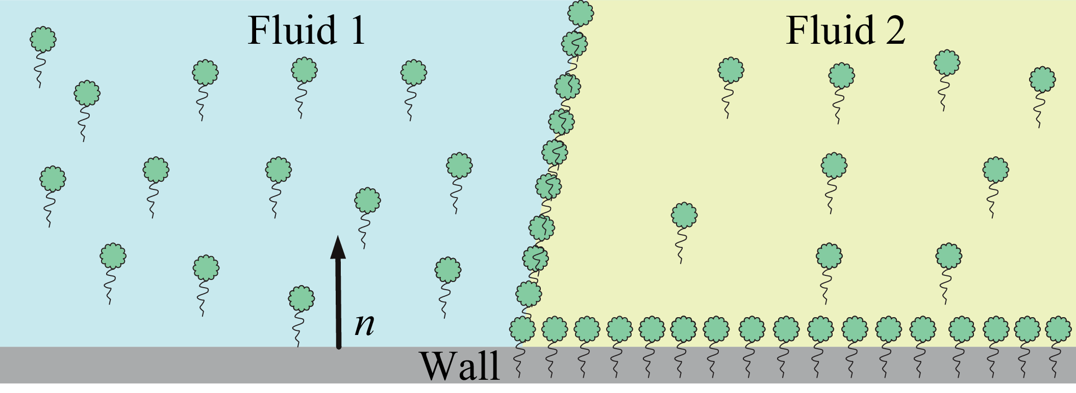
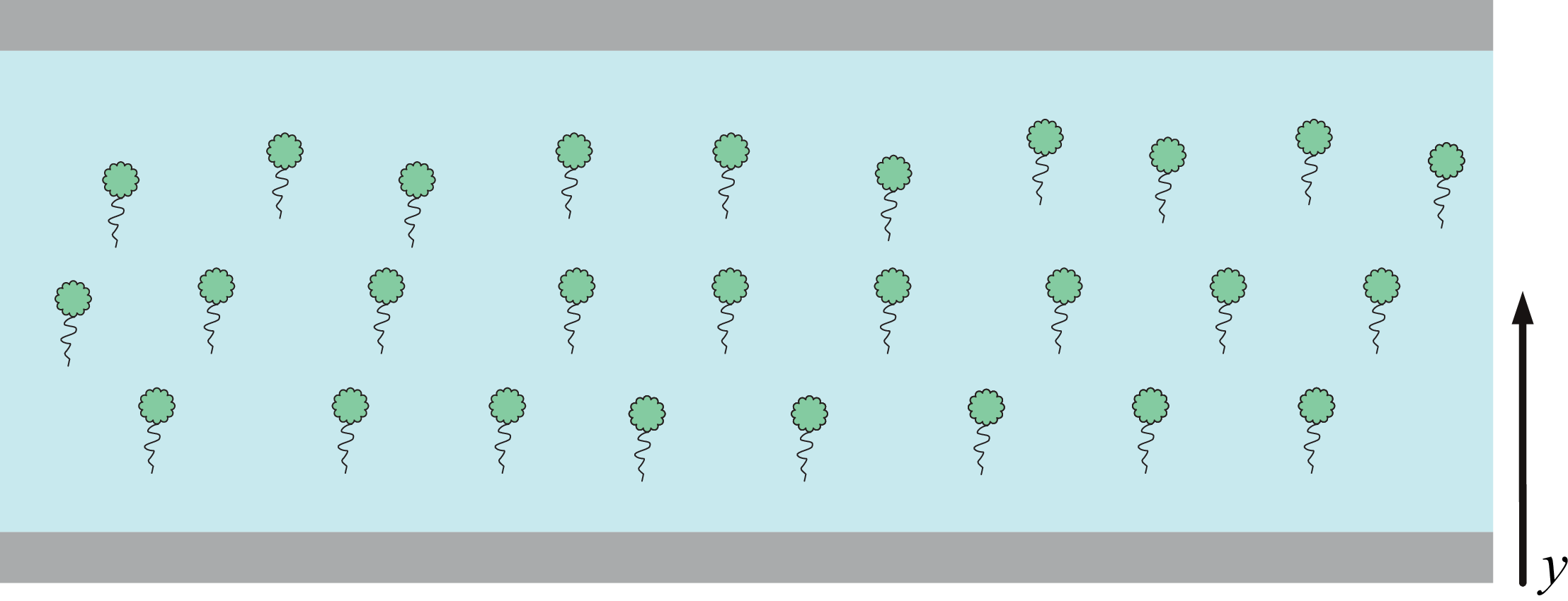
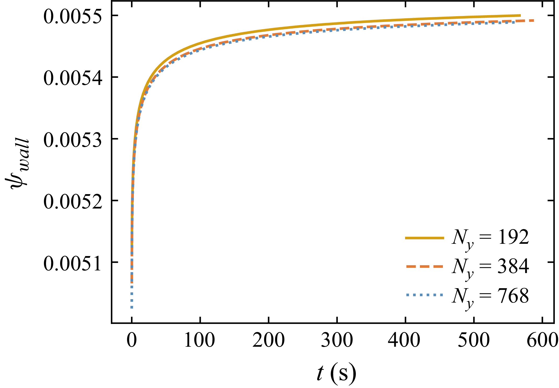
 ψwall
ψwall Ny=384
 Ny=768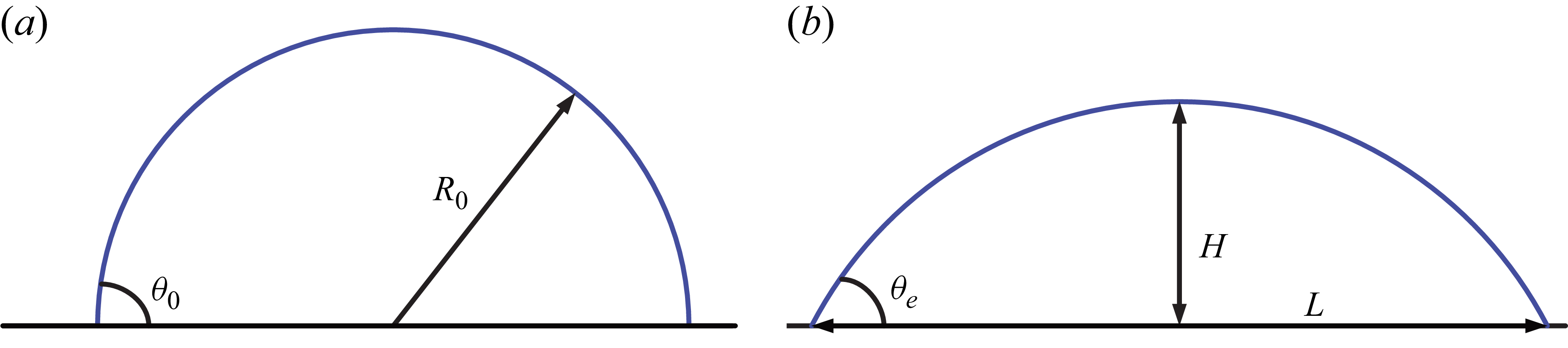
 R0
R0 θ0
θ0 θe
θe L
L H
H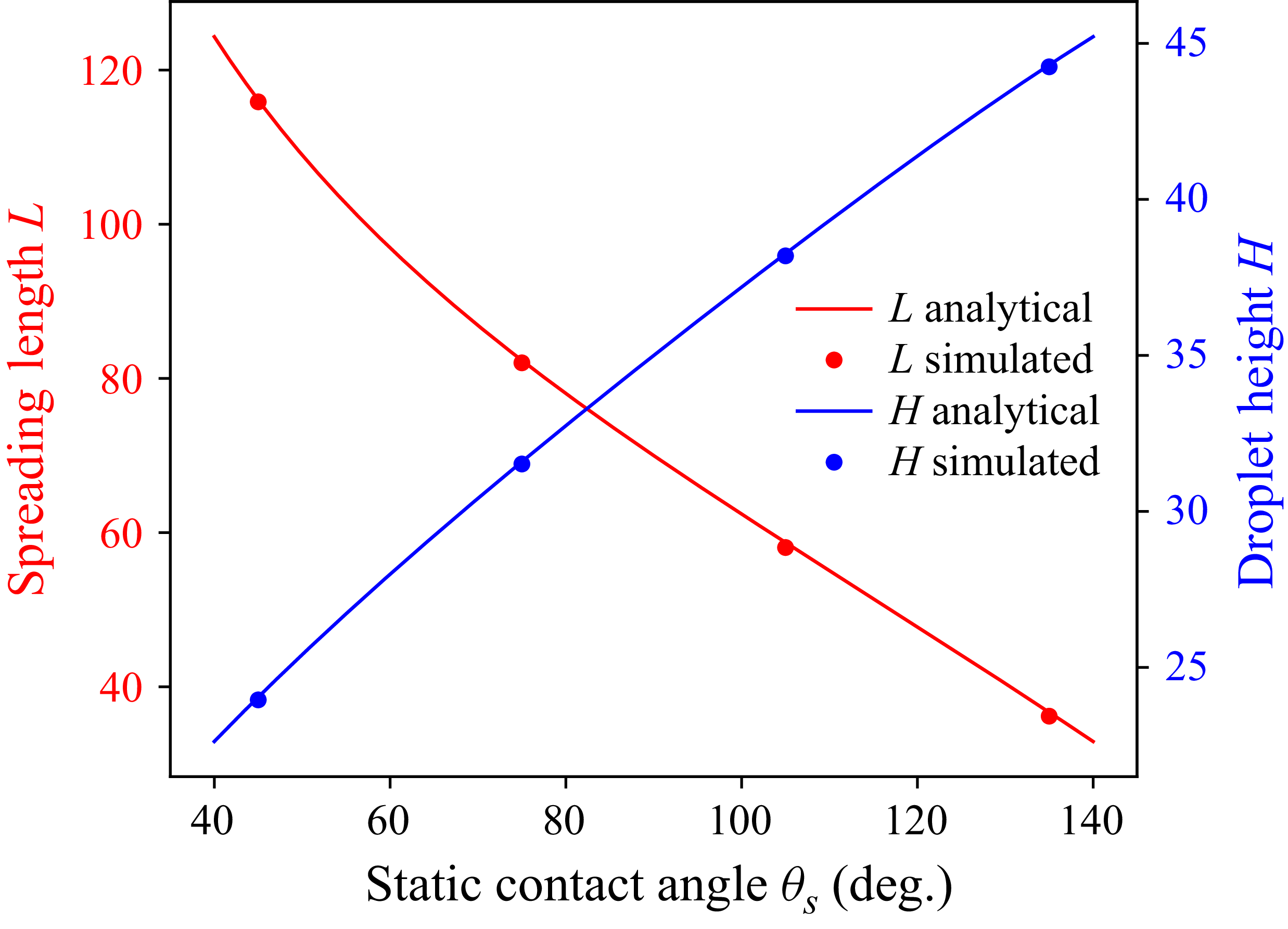
 L
L H
H θs
θs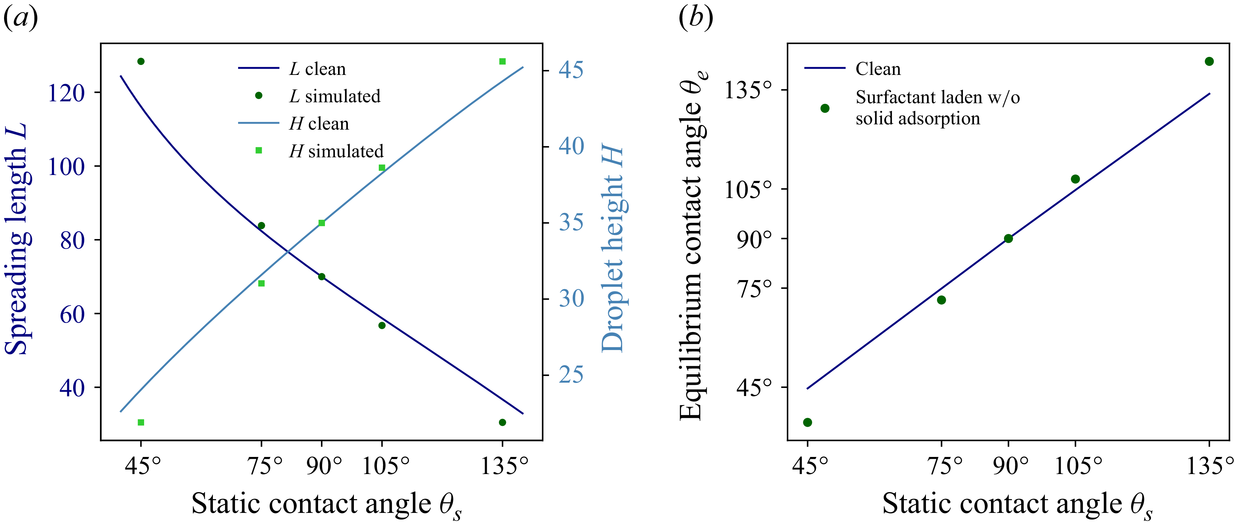
 L
L H
H θs
θs θe
θe θs
θs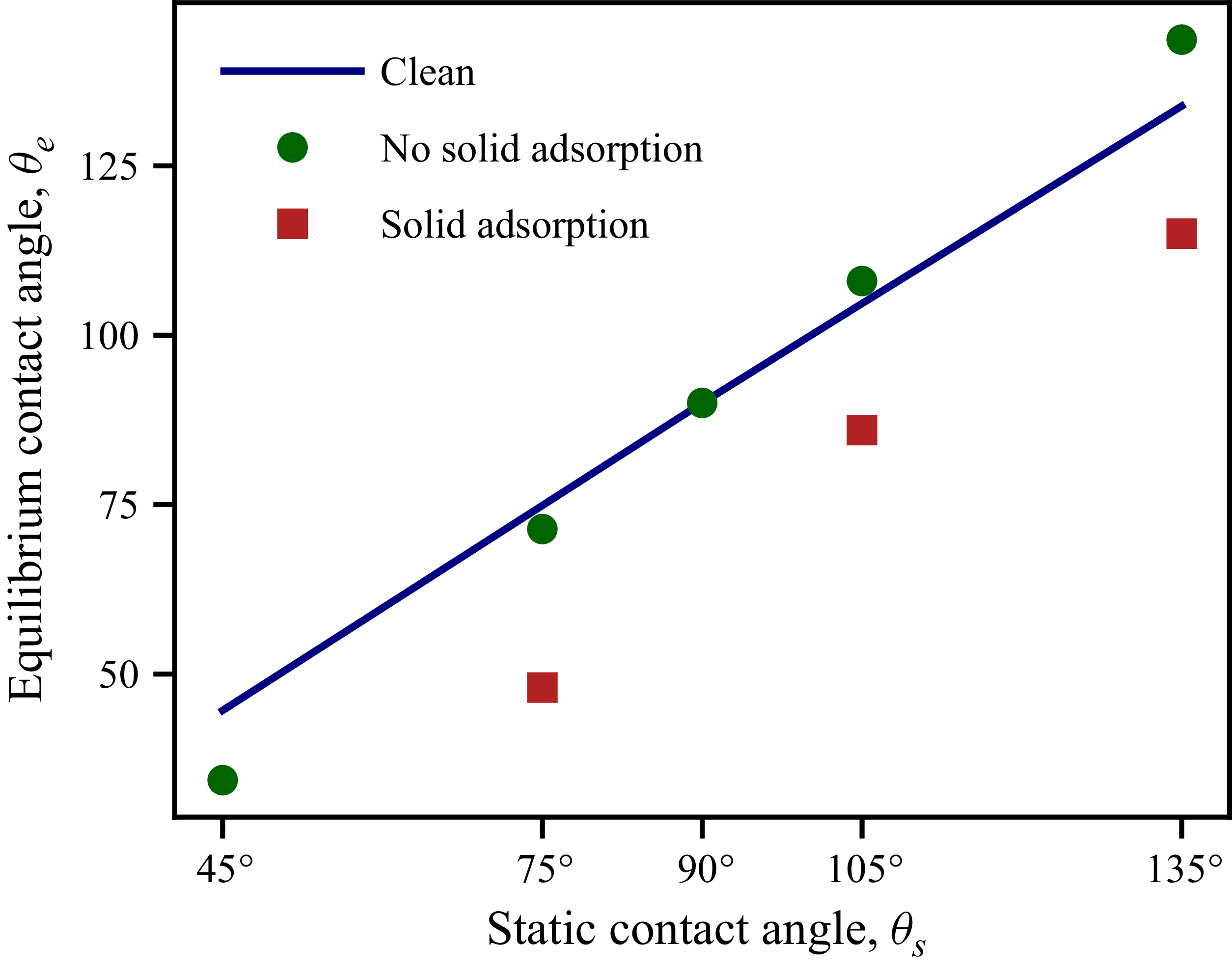
 θe
θe θs
θs
 θe
θe 75∘
75∘ θe
θe 135∘
135∘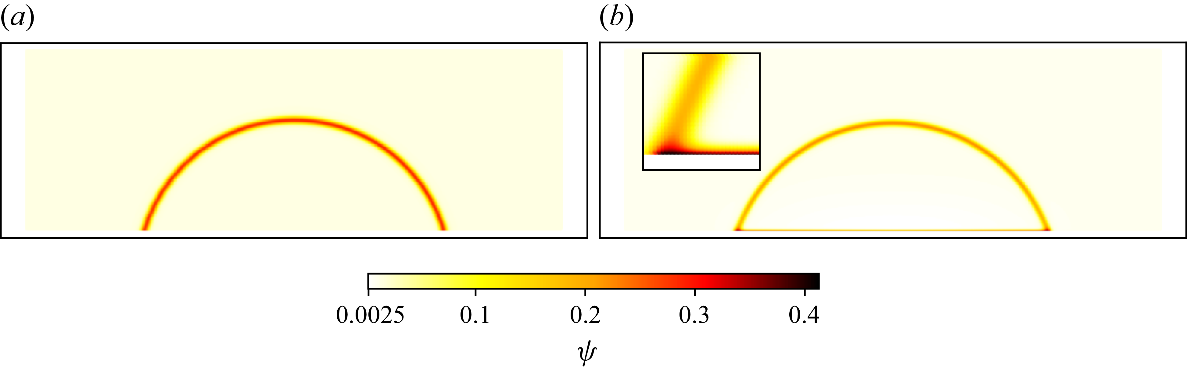
 θe
θe 75∘
75∘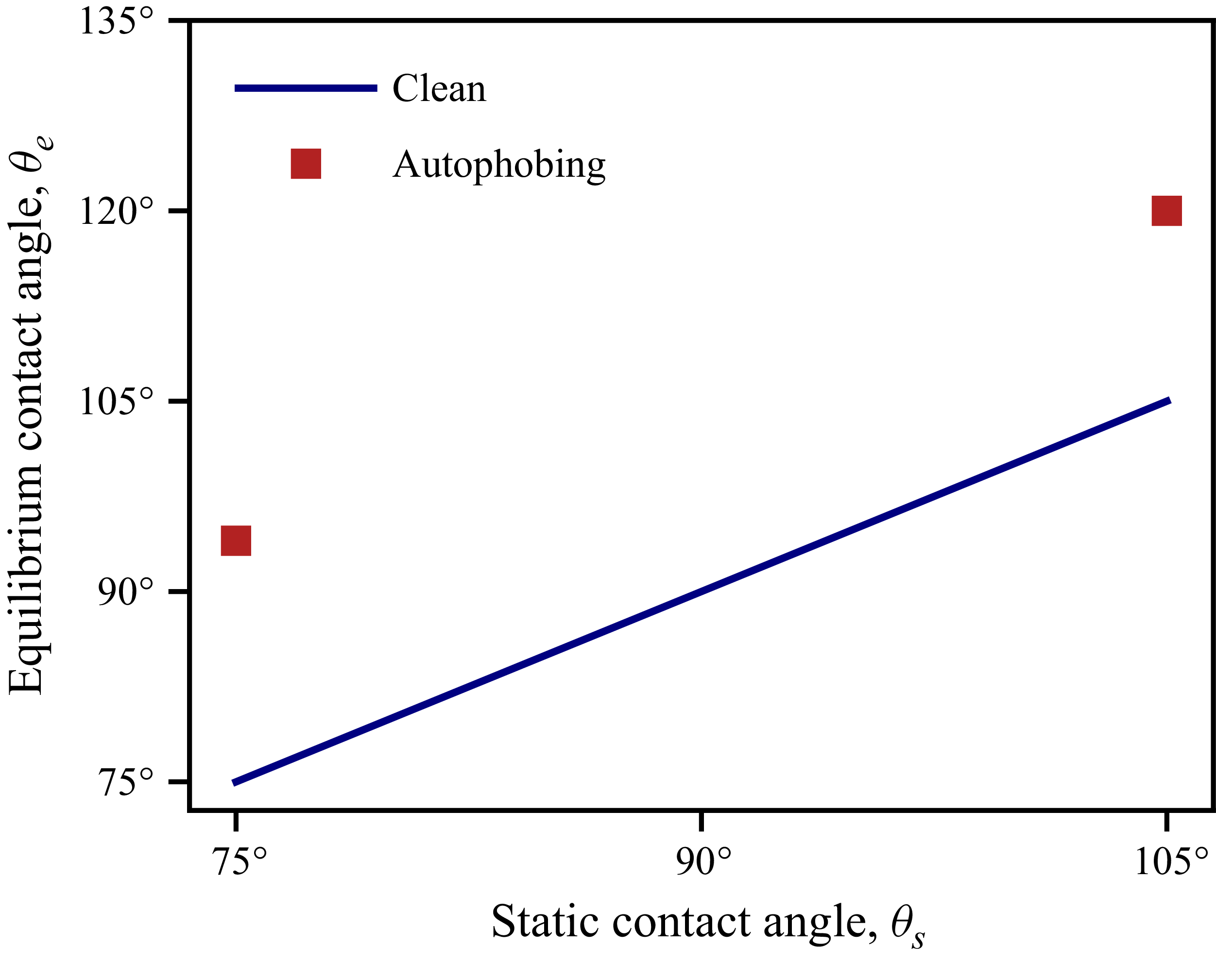
 θe
θe θs
θs
 75∘
75∘ 94∘
94∘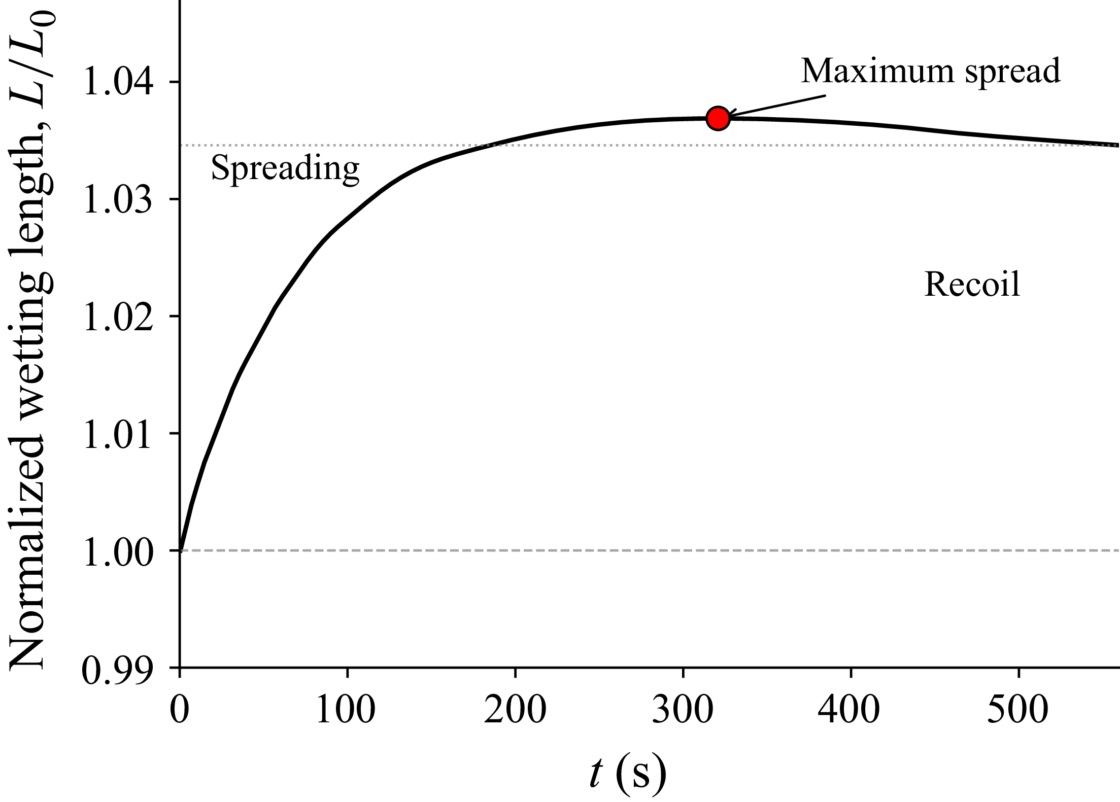
 L/L0
L/L0 βsg=0.9
 βsl=0.01
 θ0=75∘
 t≈321
t≈321 L0
L0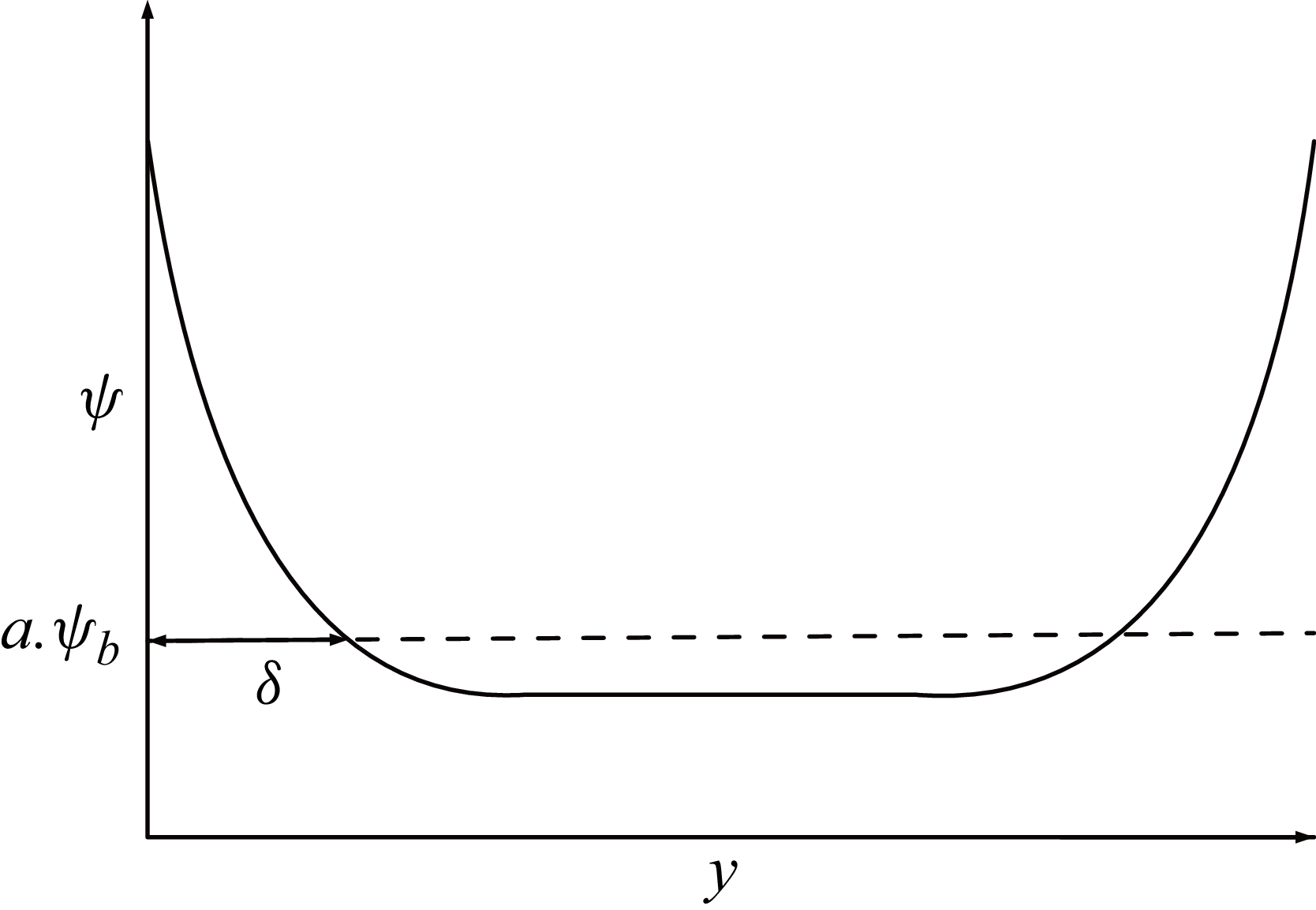
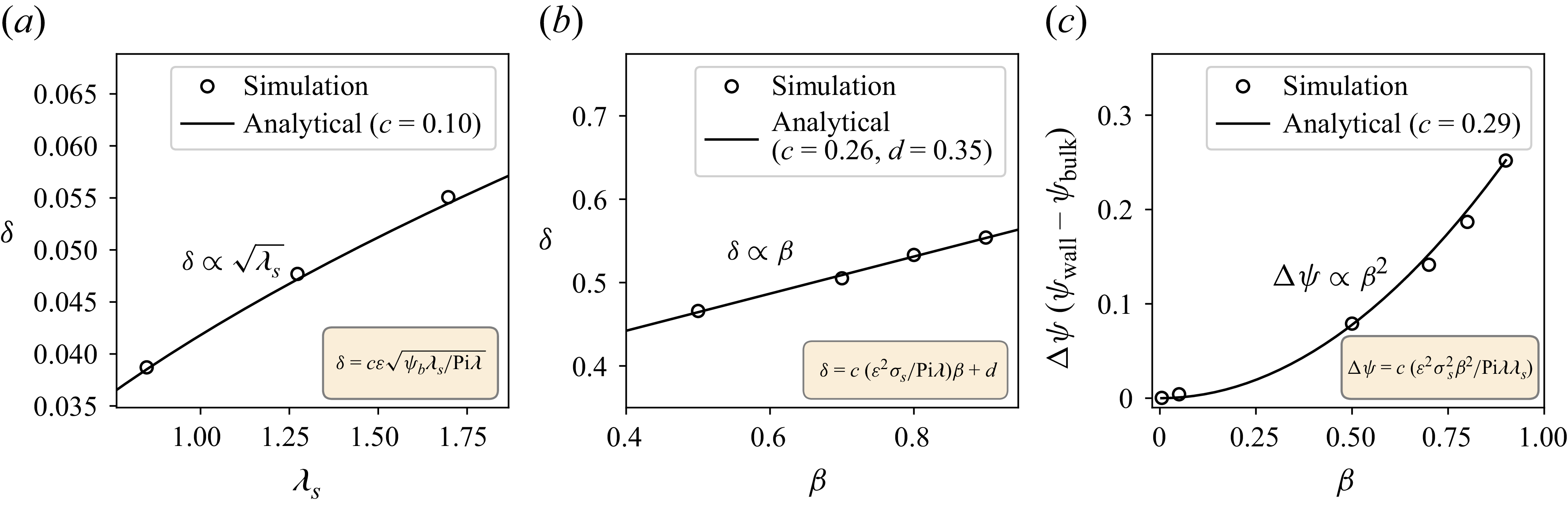
 δ
δ λs
λs δ
δ β
β Δψ
Δψ β
β β
β a
a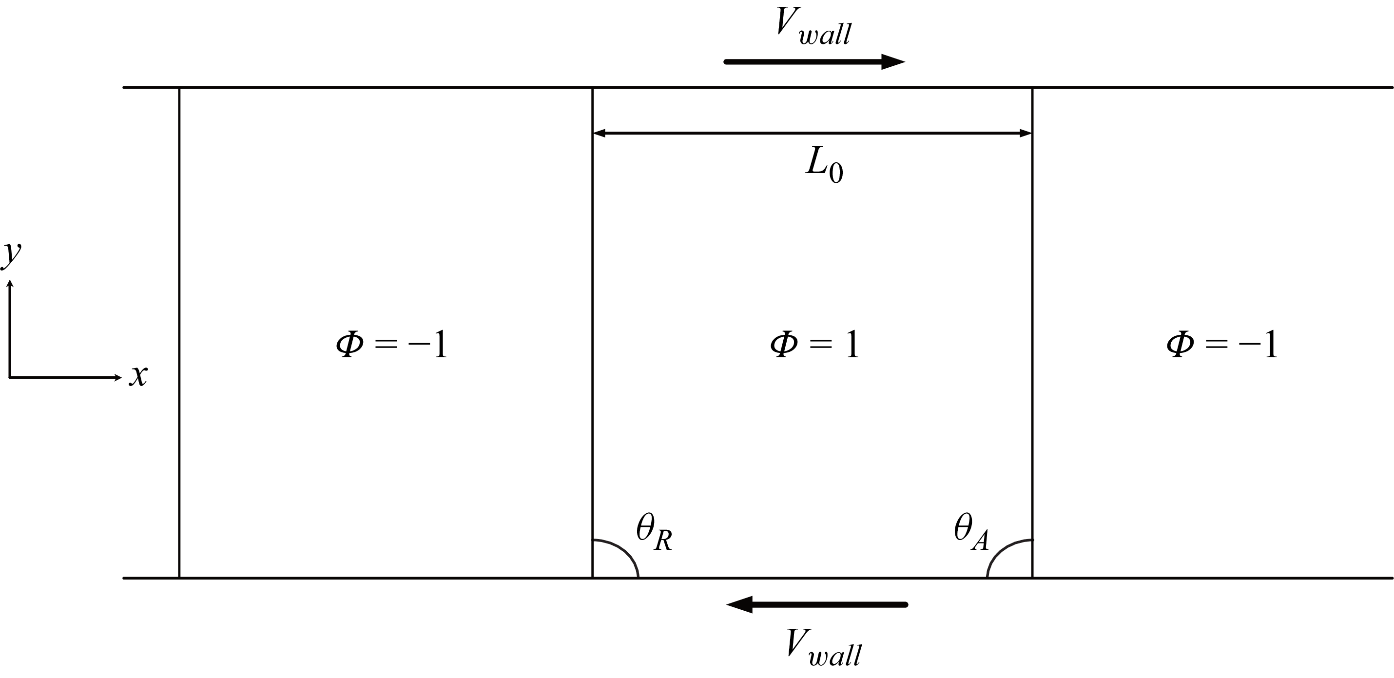

 Bsl=0.9
 Bsg=0.9
 Ca=0.02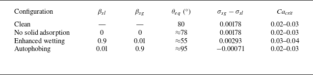
 θeq
θeq (σsg−σsl)
 Cacrit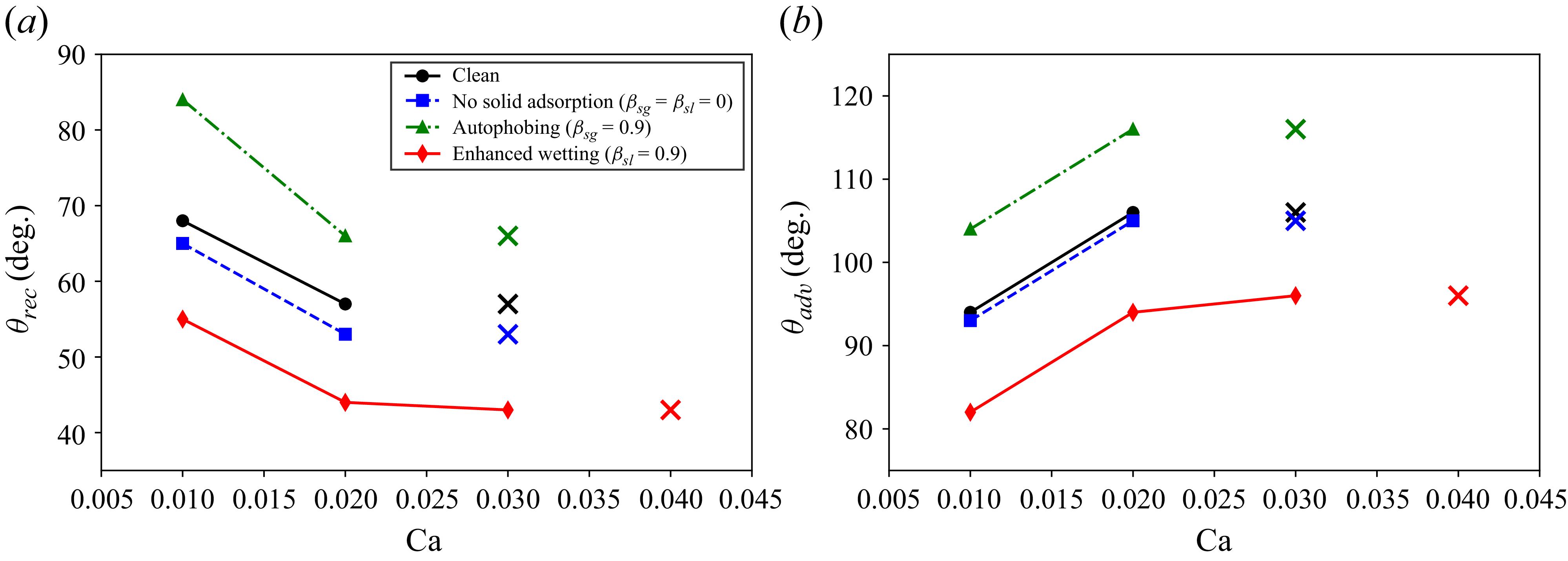
 βsl=0.9
 βsg=βsl=0
 βsg=0.9
 Ca=0.01
 0.02
0.02 Ca=0.03
 ×
× Ca=0.04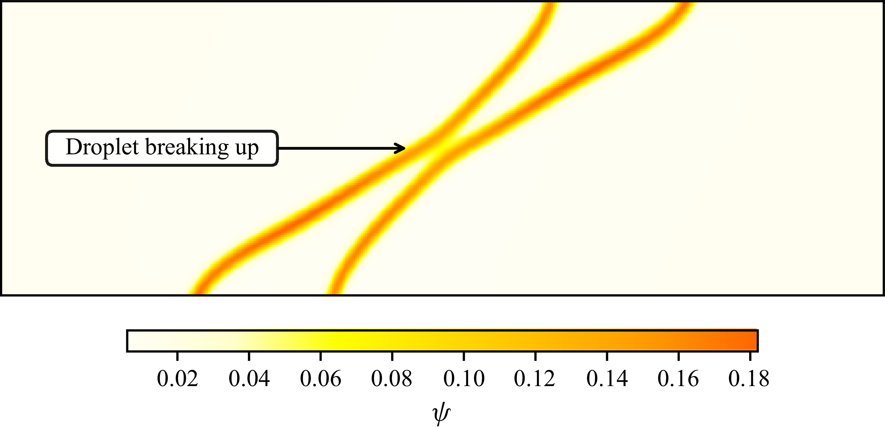
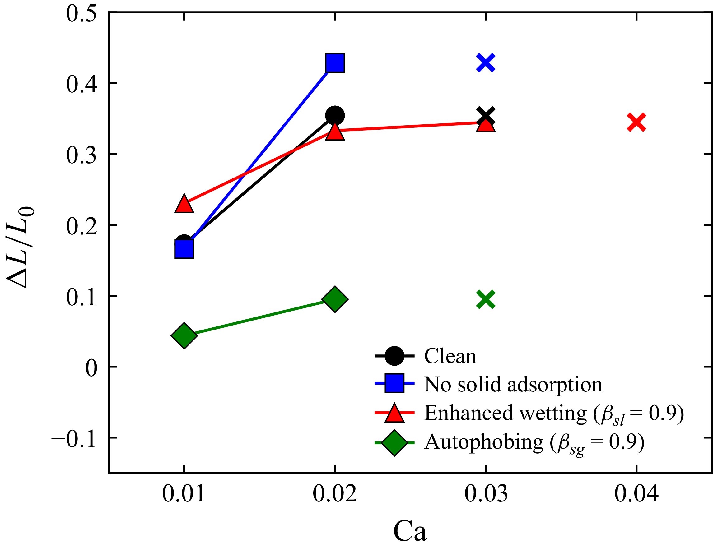
 ΔL/L0
ΔL/L0 βsl=0.9
 βsg=0.9
 ×
× Ca=0.03
 Ca=0.04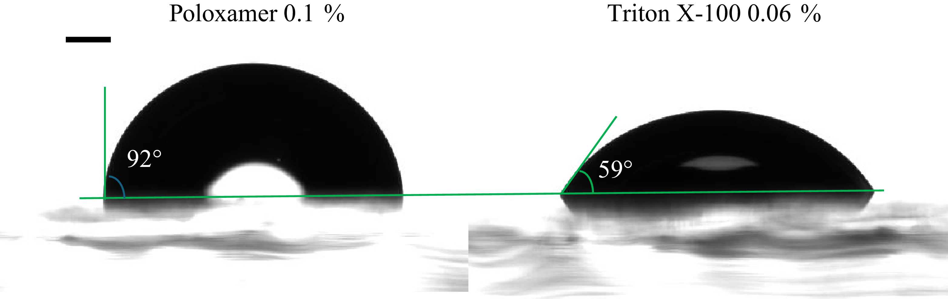
 98∘
98∘ 92∘
92∘ 59∘
59∘
 σe/σ0
σe/σ0 ψb
ψb λs
λs c1
c1 R2
R2 λs
λs
 Open access

