


1 Introduction
The index of a pair of projections introduced in [Reference Kato36, Reference Brown, Douglas and Fillmore21, Reference Avron, Seiler and Simon6] and explored further in [Reference Avron, Seiler and Simon7] is an integer-valued index that can be associated with two projections
 $P,Q$
on a Hilbert space whenever their difference is compact:
$P,Q$
on a Hilbert space whenever their difference is compact:
 $$ \begin{align*} \operatorname{index}(P,Q) = \dim \left( \operatorname{im}(P)\cap\ker(Q) \right) - \dim \left( \operatorname{im}(Q)\cap\ker(P) \right) \in \mathbb{Z}. \end{align*} $$
It is ‘topological’ in the sense that it is invariant under compact and norm-continuous deformations. In the case where one of the projections is a unitary conjugate of the other,
 $Q = U^\ast P U$
, the index reduces to a Fredholm index of
$Q = U^\ast P U$
, the index reduces to a Fredholm index of
 $PUP+P^\perp $
.
$PUP+P^\perp $
.
Since its introduction, this notion has been intimately connected to the quantum Hall effect. It is indeed one of the possible expressions for the Hall conductance, when the currents are driven by the adiabatic increase of a magnetic flux through the two-dimensional electron gas. The physical meaning of P is that of a Fermi projection whenever the Fermi energy lies in a spectral gap or a mobility gap [Reference Aizenman and Michele Graf1]. In particular, this picture is valid in a noninteracting setting where the many-body ground state reduces to a one-body projection, see [Reference Michele Graf30] for an overview and further references. This concept was eventually generalized to yield the index of all entries of the Kitaev periodic table of topological insulators [Reference Katsura and Koma37, Reference Katsura and Koma38].
There have been various attempts of generalizing the index of a pair of projections to an interacting setting where the state is not simply given by a projection in Hilbert space, most notably [Reference Bachmann, Bols, De Roeck and Fraas9] in an arbitrarily large finite volume followed by [Reference Kapustin and Sopenko33] in the infinite volume setting, where quantization can be proved under the assumption of invertibility of the initial state. In both cases, the attention is on the Hall effect.
In this work, we introduce a generalization of the above indices which is defined in a completely abstract setting. It is associated with two pure states
 $(\omega _1,\omega _2)$
of a C*-algebra
$(\omega _1,\omega _2)$
of a C*-algebra
 ${{\mathcal A}}$
that are related by an inner automorphism, in the presence of a
${{\mathcal A}}$
that are related by an inner automorphism, in the presence of a
 $U(1)$
symmetry. Specifically, when
$U(1)$
symmetry. Specifically, when
 $\omega _2 = \omega _1\circ \mathrm {Ad}_u$
, where
$\omega _2 = \omega _1\circ \mathrm {Ad}_u$
, where
 $u\in {{\mathcal A}}$
is unitary the index is given by
$u\in {{\mathcal A}}$
is unitary the index is given by
 $$ \begin{align} \mathcal{N}_\rho(\omega_1,\omega_2) := \operatorname{i}\omega_1\left(u^\ast \delta^\rho (u)\right). \end{align} $$
where
 $\delta ^\rho $
is the generator of the
$\delta ^\rho $
is the generator of the
 $U(1)$
-symmetry. We prove, among other things, that the index is integer valued, operator-norm-continuous, and invariant under deformations by symmetric automorphisms. We also show that if the algebra is chosen to be the CAR algebra describing Fermions and if the two states are quasi-free, then our index reduces to the index of a pair of projections. Therefore, this new index of a pair of pure states generalizes [Reference Avron, Seiler and Simon7], as well as the noncommutative geometric approach of [Reference Bellissard, van Elst and Schulz-Baldes17].
$U(1)$
-symmetry. We prove, among other things, that the index is integer valued, operator-norm-continuous, and invariant under deformations by symmetric automorphisms. We also show that if the algebra is chosen to be the CAR algebra describing Fermions and if the two states are quasi-free, then our index reduces to the index of a pair of projections. Therefore, this new index of a pair of pure states generalizes [Reference Avron, Seiler and Simon7], as well as the noncommutative geometric approach of [Reference Bellissard, van Elst and Schulz-Baldes17].
We then turn to the quantum Hall effect. Echoing [Reference Kapustin and Sopenko33], we prove that the piercing of a magnetic flux from
 $0$
to
$0$
to
 $2\pi $
starting from an invertible state corresponds to a situation where the many-body index is well-defined. The technical part here uses adiabatic flux insertion à la Laughlin [Reference Laughlin40] extended to the many-body setting in [Reference Bachmann, Bols and Rahnama10]. Unlike there, we focus on charge conservation rather than time-reversal symmetry. In this context, the many-body index equals the charge deficiency of the final state with respect to the initial state, and so to the Hall conductance by the Laughlin argument. This places the Hall index into a very general C*-algebraic framework which is valid for both interacting and noninteracting fermionic systems, generalizing previous expressions [Reference Bachmann, Bols, De Roeck and Fraas9, Reference Kapustin and Sopenko33] and placing them in a functional analytic framework which complements other approaches using algebraic topology [Reference Kapustin and Sopenko34, Reference Artymowicz, Kapustin and Sopenko3].
$2\pi $
starting from an invertible state corresponds to a situation where the many-body index is well-defined. The technical part here uses adiabatic flux insertion à la Laughlin [Reference Laughlin40] extended to the many-body setting in [Reference Bachmann, Bols and Rahnama10]. Unlike there, we focus on charge conservation rather than time-reversal symmetry. In this context, the many-body index equals the charge deficiency of the final state with respect to the initial state, and so to the Hall conductance by the Laughlin argument. This places the Hall index into a very general C*-algebraic framework which is valid for both interacting and noninteracting fermionic systems, generalizing previous expressions [Reference Bachmann, Bols, De Roeck and Fraas9, Reference Kapustin and Sopenko33] and placing them in a functional analytic framework which complements other approaches using algebraic topology [Reference Kapustin and Sopenko34, Reference Artymowicz, Kapustin and Sopenko3].
We point out immediately that the invertibility assumption appears in two roles that are very distinct from each other. It first plays a role as a tool that allows us to ensure that the state is the gapped ground state of a so-called parent Hamiltonian. Secondly, it is crucial in concluding that the defect state obtained after flux insertion is locally comparable to the initial state, namely that the two differ only in the vicinity of the puncture and not at infinity. While the first role could be bypassed in a physical setting where the state is given as a gapped ground state, the second one appears fundamental. Indeed, it is that very assumption that ensures that the state has integer quantum Hall conductance as opposed to fractional conductance. In the latter case, the initial state is expected to have nontrivial superselection sectors corresponding to anyonic excitations (see [Reference Ogata43] for one possible meaning of these terms and [Reference Fröhlich, Studer and Thiran25] for an overview of anyons in the fractional quantum Hall effect) and these cannot be realized upon an invertible state [Reference Kitaev39, Reference Bachmann, Getz, Naaijkens and Wray15].
Let us briefly discuss other approaches to (integer) quantization in the interacting quantum Hall effect. In the single particle picture, charge deficiency, charge transport and linear response coincide [Reference Laughlin40, Reference Avron, Seiler and Simon6, Reference Michele Graf30]. This equivalence continues to hold in the interacting picture [Reference Bachmann, Bols, De Roeck and Fraas9, Reference Kapustin and Sopenko33], where quantization of the Hall conductance was proved in [Reference Hastings and Michalakis31, Reference Bachmann, Bols, De Roeck and Fraas8], see also [Reference Bachmann, De Roeck and Fraas12, Reference Monaco and Teufel42] for the validity of linear response. While the above assume the presence of a gap, this assumption is proved to hold in a perturbative setting in [Reference Giuliani, Mastropietro and Porta28], while it is not needed if one considers nonequilibrium almost steady states [Reference Wesle, Marcelli, Miyao, Monaco and Teufel49, Reference Teufel and Wesle46].
The paper is organized as follows. In Section 2, we describe the general algebraic setting, introduce the notion of two pure states being
 $\rho $
-locally comparable, (see Definition 2.3) and define the index
$\rho $
-locally comparable, (see Definition 2.3) and define the index
 ${\mathcal N}_\rho (\omega _1,\omega _2)$
. If
${\mathcal N}_\rho (\omega _1,\omega _2)$
. If
 $\rho _t$
is a
$\rho _t$
is a
 $U(1)$
-symmetry, then
$U(1)$
-symmetry, then
 $$ \begin{align*}{\mathcal N}_\rho(\omega_1,\omega_2)\in \mathbb{Z}.\end{align*} $$
In Section 2.2, we consider the Fermionic algebra
 ${\mathcal A}=\mathrm {CAR}(\cal H)$
on a one-particle Hilbert space
${\mathcal A}=\mathrm {CAR}(\cal H)$
on a one-particle Hilbert space
 $\mathcal {H}$
. For
$\mathcal {H}$
. For
 $P,Q$
two orthogonal projections on
$P,Q$
two orthogonal projections on
 $\mathcal H$
and
$\mathcal H$
and
 $\omega _P, \omega _Q$
their corresponding quasi-free states on
$\omega _P, \omega _Q$
their corresponding quasi-free states on
 ${\mathcal A}$
, we show that if
${\mathcal A}$
, we show that if
 $P-Q$
is trace class then
$P-Q$
is trace class then
 $$ \begin{align*}{\mathcal N}_\rho(\omega_P,\omega_Q) = \mathrm{index}(P,Q), \end{align*} $$
the index of a pair of projection. Section 3 focusses on the quantum Hall effect in an interacting setting where the two states are an initial invertible state and a defect state obtained from the initial one by inserting a unit of flux at the origin. Then the charge deficiency, and therefore the Hall conductance, is given by
 $$ \begin{align*}\mathcal{N}_{\rho\otimes\mathrm{id}} (\hat \omega, \hat\omega^D) \in \mathbb{Z} \end{align*} $$
where
 $\hat \cdot $
corresponds to a stacking operation associated to invertible states. The fact that we pick
$\hat \cdot $
corresponds to a stacking operation associated to invertible states. The fact that we pick
 $\rho \otimes \mathrm {id}$
rather than the stacked
$\rho \otimes \mathrm {id}$
rather than the stacked
 $\hat {\rho }$
means that we measure only the charge transported in the original system, rather than in the full, stacked system. We then show in Section 4 that this index covers gapped ground states of interacting Hamiltonian as well, and that in the quasi-free case it coincides with a single-particle spectral flow.
$\hat {\rho }$
means that we measure only the charge transported in the original system, rather than in the full, stacked system. We then show in Section 4 that this index covers gapped ground states of interacting Hamiltonian as well, and that in the quasi-free case it coincides with a single-particle spectral flow.
2 Abstract index theory
2.1 The index of a pair of pure states
Let
 $\mathcal {A}$
be a unital C*-algebra. In later sections we shall apply the theory to
$\mathcal {A}$
be a unital C*-algebra. In later sections we shall apply the theory to
 $\mathcal {A}=\operatorname {CAR}(\mathcal {H})$
for some separable Hilbert space
$\mathcal {A}=\operatorname {CAR}(\mathcal {H})$
for some separable Hilbert space
 $\mathcal {H}$
but in fact throughout this section no assumptions on
$\mathcal {H}$
but in fact throughout this section no assumptions on
 $\mathcal {A}$
will be made. We denote by
$\mathcal {A}$
will be made. We denote by
 $\mathcal {U}(\mathcal {A})$
the set of unitary elements of
$\mathcal {U}(\mathcal {A})$
the set of unitary elements of
 $\mathcal {A}$
. A state
$\mathcal {A}$
. A state
 $\omega : {\mathcal A} \to \mathbb C$
is a positive (i.e.,
$\omega : {\mathcal A} \to \mathbb C$
is a positive (i.e.,
 $\omega (a^{*} a)\geq 0$
for all
$\omega (a^{*} a)\geq 0$
for all
 $a\in \mathcal {A}$
) linear functional on
$a\in \mathcal {A}$
) linear functional on
 ${\mathcal A}$
with
${\mathcal A}$
with ![]() ; the space of all states shall be denoted
; the space of all states shall be denoted
 $\mathcal S({\mathcal A})$
. The condition
$\mathcal S({\mathcal A})$
. The condition ![]() is equivalent to the normalization
is equivalent to the normalization
 $\|\omega \| =1$
, where the norm is given by
$\|\omega \| =1$
, where the norm is given by
 $$ \begin{align*} \left\Vert \omega \right\Vert := \sup\left(\{ \left\lvert {\omega(a)} \right\rvert | a\in\mathcal{A} : \left\Vert a \right\Vert\leq 1\}\right). \end{align*} $$
In other words, all states are on the unit sphere of
 ${{\mathcal A}}^{*}$
and so
${{\mathcal A}}^{*}$
and so
 $\mathcal S({\mathcal A})$
is a weakly*-compact and convex subset of
$\mathcal S({\mathcal A})$
is a weakly*-compact and convex subset of
 ${\mathcal A}^{*}$
. The extreme points of
${\mathcal A}^{*}$
. The extreme points of
 $\mathcal S({\mathcal A})$
are called pure states and their collection is denoted by
$\mathcal S({\mathcal A})$
are called pure states and their collection is denoted by
 ${\mathcal P}({{\mathcal A}})$
.
${\mathcal P}({{\mathcal A}})$
.
Definition 2.1 (locally comparable pair of pure states).
Let
 $\omega _1,\omega _2\in \mathcal {P}(\mathcal {A})$
be a pair of pure states. We say that the pair
$\omega _1,\omega _2\in \mathcal {P}(\mathcal {A})$
be a pair of pure states. We say that the pair
 $(\omega _1,\omega _2)$
is locally comparable iff there exists some
$(\omega _1,\omega _2)$
is locally comparable iff there exists some
 $u\in \mathcal {U}(\mathcal {A})$
such that
$u\in \mathcal {U}(\mathcal {A})$
such that
 $$ \begin{align} \omega_2 = \omega_1 \circ \operatorname{Ad}_{u}\!. \end{align} $$
Here and in the sequel,
 $\operatorname {Ad}_{u}$
denotes the automorphism
$\operatorname {Ad}_{u}$
denotes the automorphism
 $\operatorname {Ad}_{u}(a) = u^{*} a u$
. In other words,
$\operatorname {Ad}_{u}(a) = u^{*} a u$
. In other words,
 $\omega _1$
and
$\omega _1$
and
 $\omega _2$
are locally comparable iff they are inner-automorphism equivalent.
$\omega _2$
are locally comparable iff they are inner-automorphism equivalent.
Remark 2.2. The intuition we have in mind for two pure states to be locally comparable is that their difference is “compact” in a vague sense. Since
 $$ \begin{align*} \omega_2 -\omega_1 = \omega_1\circ \left(\operatorname{Ad}_{u}-\mathrm{id}\right), \end{align*} $$
if
 $\mathcal {A}=\operatorname {CAR}(\mathcal {H})$
for some Hilbert space
$\mathcal {A}=\operatorname {CAR}(\mathcal {H})$
for some Hilbert space
 $\mathcal {H}$
, then
$\mathcal {H}$
, then
 $\mathcal {A}$
may be considered as the operator norm limit of finite-rank (but not necessarily quadratic) observables, and as such, since
$\mathcal {A}$
may be considered as the operator norm limit of finite-rank (but not necessarily quadratic) observables, and as such, since
 $u\in \mathcal {U}(\mathcal {A})$
, we should consider
$u\in \mathcal {U}(\mathcal {A})$
, we should consider ![]() and hence also
and hence also
 $\operatorname {Ad}_{u}-\mathrm {id}$
to be (the many-body analog of) compact. Then by the ideal property, the whole expression
$\operatorname {Ad}_{u}-\mathrm {id}$
to be (the many-body analog of) compact. Then by the ideal property, the whole expression
 $\omega _1\circ \left (\operatorname {Ad}_{u}-\mathrm {id}\right )$
is.
$\omega _1\circ \left (\operatorname {Ad}_{u}-\mathrm {id}\right )$
is.
Back to the case of a general C*-algebra
 $\mathcal {A}$
, when two pure states
$\mathcal {A}$
, when two pure states
 $\omega _1,\omega _2$
are locally comparable, we want to measure how different they are, with the expectation that if they are path-connected (in
$\omega _1,\omega _2$
are locally comparable, we want to measure how different they are, with the expectation that if they are path-connected (in
 $\mathcal {P}(\mathcal {A})$
) they should not be different at all. This is the case when
$\mathcal {P}(\mathcal {A})$
) they should not be different at all. This is the case when
 $u\in \mathcal {U}_0(\mathcal {A})$
, that is, when u may be continuously deformed to
$u\in \mathcal {U}_0(\mathcal {A})$
, that is, when u may be continuously deformed to ![]() , whence we get a continuous deformation of
, whence we get a continuous deformation of
 $\omega _2$
to
$\omega _2$
to
 $\omega _1$
. However, there are C*-algebras where
$\omega _1$
. However, there are C*-algebras where
 $\pi _0(\mathcal {U}(\mathcal {A}))\neq \{0\}$
(for example
$\pi _0(\mathcal {U}(\mathcal {A}))\neq \{0\}$
(for example
 $C({\mathbb S}^1)$
). It will turn out that we are not quite interested in such obstructions. Rather, in many interesting cases (such as UHF algebras),
$C({\mathbb S}^1)$
). It will turn out that we are not quite interested in such obstructions. Rather, in many interesting cases (such as UHF algebras),
 $\pi _0(\mathcal {U}(\mathcal {A}))=\{0\}$
. Then, to gauge a topological obstruction we impose a further symmetry constraint.
$\pi _0(\mathcal {U}(\mathcal {A}))=\{0\}$
. Then, to gauge a topological obstruction we impose a further symmetry constraint.
Let
 $\{\rho _t\}_{t\in \mathbb {R}}\subseteq \operatorname {Aut}(\mathcal {A})$
be a strongly continuous one-parameter group of *-automorphisms. Its generator
$\{\rho _t\}_{t\in \mathbb {R}}\subseteq \operatorname {Aut}(\mathcal {A})$
be a strongly continuous one-parameter group of *-automorphisms. Its generator
 $\delta ^\rho $
, given by
$\delta ^\rho $
, given by
 $$ \begin{align*} \delta^\rho := \mathrm{s-lim}_{t\to0^+}\frac{1}{t}\left(\rho_t-\mathrm{id}\right) \end{align*} $$
is a *-derivation. In general
 $\rho _t$
is not expected to be inner and
$\rho _t$
is not expected to be inner and
 $\delta ^\rho $
is not expected to be bounded. As such, we must consider
$\delta ^\rho $
is not expected to be bounded. As such, we must consider
 $\delta ^\rho $
together with its domain
$\delta ^\rho $
together with its domain
 $$ \begin{align*} \mathcal{D}(\delta^\rho) \equiv \{a\in\mathcal{A} | \lim_{t\to0^+}\frac{1}{t}\left(\rho_t(a)-a\right)\text{ exists in }\mathcal{A}\}. \end{align*} $$
With this, we refine the notion of locally comparable pure states as follows.
Definition 2.3 (
 $\rho $
-locally comparable pair of pure states).
$\rho $
-locally comparable pair of pure states).

Let
 $\rho _t$
be as above and
$\rho _t$
be as above and
 $(\omega _1,\omega _2)$
be a pair of pure states. We say that this pair is
$(\omega _1,\omega _2)$
be a pair of pure states. We say that this pair is
 $\rho $
-locally comparable iff there exists some
$\rho $
-locally comparable iff there exists some
 $u\in \mathcal {U}(\mathcal {A})\cap \mathcal {D}(\delta ^\rho )$
such that
$u\in \mathcal {U}(\mathcal {A})\cap \mathcal {D}(\delta ^\rho )$
such that
 $$ \begin{align*} \omega_2 = \omega_1 \circ \operatorname{Ad}_{u}\!. \end{align*} $$
We now have all the definitions to set up our index.
Definition 2.4 (The index of a locally comparable pair of
$\rho $
-invariant pure states).

Let
 $\rho _t$
be as above and
$\rho _t$
be as above and
 $(\omega _1,\omega _2)$
be a pair of
$(\omega _1,\omega _2)$
be a pair of
 $\rho $
-locally comparable pure states. Assume moreover that both
$\rho $
-locally comparable pure states. Assume moreover that both
 $\omega _1$
and
$\omega _1$
and
 $\omega _2$
are
$\omega _2$
are
 $\rho $
-invariant, that is,
$\rho $
-invariant, that is,
 $$ \begin{align*} \omega_j \circ \rho_t = \omega_j \qquad (t\in\mathbb{R},j=1,2). \end{align*} $$
Then the index of the pair
 $(\omega _1,\omega _2)$
is defined as
$(\omega _1,\omega _2)$
is defined as
 $$ \begin{align} \mathcal{N}_\rho(\omega_1,\omega_2) := \operatorname{i}\omega_1\left(u^\ast \delta^\rho (u)\right) \end{align} $$
where
 $u\in \mathcal {D}(\delta ^\rho )$
is any unitary which obeys
$u\in \mathcal {D}(\delta ^\rho )$
is any unitary which obeys
 $\omega _2=\omega _1\circ \operatorname {Ad}_{u}$
.
$\omega _2=\omega _1\circ \operatorname {Ad}_{u}$
.
We note that in general there is no reason for the unitary u above to be
 $\rho _t$
-invariant; see Remark 3.22(iii) for an explicit example. Indeed, if this happens, then
$\rho _t$
-invariant; see Remark 3.22(iii) for an explicit example. Indeed, if this happens, then
 $\delta ^\rho (u) = 0$
and so
$\delta ^\rho (u) = 0$
and so
 $\mathcal {N}_\rho (\omega _1,\omega _2)=0$
.
$\mathcal {N}_\rho (\omega _1,\omega _2)=0$
.
The condition that the pair
 $(\omega _1,\omega _2)$
must be compatible with
$(\omega _1,\omega _2)$
must be compatible with
 $\rho $
in the above sense, namely that they are
$\rho $
in the above sense, namely that they are
 $\rho $
-locally comparable and invariant, means they are generically not path connected, which is what the index measures.
$\rho $
-locally comparable and invariant, means they are generically not path connected, which is what the index measures.
Theorem 2.5 (Properties of the index).
The index defined above has the following properties:
-
(i)
$\mathcal {N}_\rho (\omega _1,\omega _2)$
does not depend on the choice of
$u\in \mathcal {D}(\delta ^\rho )\cap \mathcal {U}(\mathcal {A})$
such that
$\omega _2=\omega _1\circ \operatorname {Ad}_{u}$
. -
(ii) If
$\rho _{2\pi }=\mathrm {id}$
, then
$\mathcal {N}_\rho (\omega _1,\omega _2)\in \mathbb {Z}$
. -
(iii)
$\mathcal {N}_\rho (\omega _1,\omega _2)$
has the following continuity property: (4)
$$ \begin{align} \left\Vert \omega_1-\omega_2 \right\Vert<2\Longrightarrow \mathcal{N}_\rho(\omega_1,\omega_2) = 0. \end{align} $$
-
(iv) For any automorphism
$\alpha $
of
${{\mathcal A}}$
such that
$\alpha \circ \delta ^\rho = \delta ^\rho \circ \alpha $
, (5)
$$ \begin{align} \mathcal{N}_\rho(\omega_1\circ\alpha,\omega_2\circ\alpha) = \mathcal{N}_\rho(\omega_1,\omega_2). \end{align} $$
-
(v)
$\mathcal {N}_\rho \left (\omega ,\omega \right ) = 0$
for any
$\rho $
-invariant pure state
$\omega \in \mathcal {P}(\mathcal {A})$
. -
(vi) If
$\omega _1,\omega _2,\omega _3$
are three pairwise
$\rho $
-locally comparable pure states, all of which are
$\rho $
-invariant, then (6)
$$ \begin{align} \mathcal{N}_\rho(\omega_1,\omega_2)+\mathcal{N}_\rho(\omega_2,\omega_3) = \mathcal{N}_\rho(\omega_1,\omega_3). \end{align} $$
-
(vii) The index is anti-symmetric
(7)
$$ \begin{align} \mathcal{N}_\rho(\omega_1,\omega_2) = -\mathcal{N}_\rho(\omega_2,\omega_1). \end{align} $$
-
(viii) We have the following additivity with respect to tensor products. Let
$\widetilde {\mathcal {A}}$
be another C*-algebra and
$\widetilde {\rho }$
as above; Let further
$\widetilde {\omega _1},\widetilde {\omega _2}$
be two
$\widetilde \rho $
-locally comparable pure states on
$\widetilde {\mathcal {A}}$
which are
$\widetilde {\rho }_t$
-invariant. Then (8)
$$ \begin{align} \mathcal{N}_{\rho\otimes\widetilde{\rho}}\left(\omega_1\otimes\widetilde{\omega_1},\omega_2\otimes\widetilde{\omega_2}\right) = \mathcal{N}_\rho(\omega_1,\omega_2) + \mathcal{N}_{\widetilde{\rho}}(\widetilde{\omega_1},\widetilde{\omega_2}). \end{align} $$


To clarify further, let us assume temporarily that
 $\mathcal {A}$
is a uniformly hyperfinite (UHF) algebra. In this case, it is well known (see, e.g., [Reference Bratteli and William Robinson19, Prop 3.2.52]) that one may find a sequence
$\mathcal {A}$
is a uniformly hyperfinite (UHF) algebra. In this case, it is well known (see, e.g., [Reference Bratteli and William Robinson19, Prop 3.2.52]) that one may find a sequence
 $\{q_n=q_n^\ast \}_n\subseteq \mathcal {A}$
such that
$\{q_n=q_n^\ast \}_n\subseteq \mathcal {A}$
such that
 $$ \begin{align*} \delta^\rho = \mathrm{s-lim}_{n\to\infty}\operatorname{i}[q_n,\cdot]. \end{align*} $$
Then it is clear that
 $$ \begin{align} \mathcal{N}_\rho(\omega_1,\omega_2) = \lim_{n}\left(\omega_1(q_n)-\omega_2(q_n)\right). \end{align} $$
Since this expression does not involve the unitary u the index is well-defined. The remainder of this subsection does not assume that
 $\mathcal {A}$
is UHF.
$\mathcal {A}$
is UHF.
Remark 2.6. If
 $(\omega _1,\omega _2)$
are
$(\omega _1,\omega _2)$
are
 $\rho $
-locally comparable and if
$\rho $
-locally comparable and if
 $\tilde \omega _2 = \omega _2\circ \mathrm {Ad}_v$
for a
$\tilde \omega _2 = \omega _2\circ \mathrm {Ad}_v$
for a
 $v\in {\mathcal U}({{\mathcal A}})$
with
$v\in {\mathcal U}({{\mathcal A}})$
with
 $\delta ^\rho (v)=0$
, then
$\delta ^\rho (v)=0$
, then
 $(\omega _1,\tilde \omega _2)$
are also
$(\omega _1,\tilde \omega _2)$
are also
 $\rho $
-locally comparable and
$\rho $
-locally comparable and
 $$ \begin{align} {\mathcal N}_\rho(\omega_1,\tilde\omega_2 ) = {\mathcal N}_\rho(\omega_1,\omega_2) \end{align} $$
by additivity (6) and
 ${\mathcal N}_\rho (\tilde \omega _2, \omega _2) = 0$
.
${\mathcal N}_\rho (\tilde \omega _2, \omega _2) = 0$
.
Proof of Theorem 2.5.
(i) If we have
 $\omega _2 = \omega _1\circ \operatorname {Ad}_{u} = \omega _1\circ \operatorname {Ad}_{v}$
for two a priori distinct unitaries
$\omega _2 = \omega _1\circ \operatorname {Ad}_{u} = \omega _1\circ \operatorname {Ad}_{v}$
for two a priori distinct unitaries
 $u,v\in \mathcal {U}(\mathcal {A})$
then this readily implies
$u,v\in \mathcal {U}(\mathcal {A})$
then this readily implies
 $\omega _1 = \omega _1 \circ \operatorname {Ad}_{u^\ast v}$
. Let us define
$\omega _1 = \omega _1 \circ \operatorname {Ad}_{u^\ast v}$
. Let us define
 $w := u^\ast v$
whence
$w := u^\ast v$
whence
 $\omega _1= \omega _1\circ \operatorname {Ad}_{w}$
. Since
$\omega _1= \omega _1\circ \operatorname {Ad}_{w}$
. Since
 $v = uw $
, we have
$v = uw $
, we have
 $$ \begin{align*} v^\ast \delta^\rho(v) = (uw)^\ast \delta^\rho (uw)= w^\ast u^\ast \delta^\rho(u) w + w^\ast \delta^\rho(w). \end{align*} $$
Applying
 $\omega _1$
to both sides of this and using the w-invariance of
$\omega _1$
to both sides of this and using the w-invariance of
 $\omega _1$
, it remains to show that
$\omega _1$
, it remains to show that
 $\omega _1(w^\ast \delta ^\rho (w)) =0$
to get the statement. Using Lemma 2.7 below we have that
$\omega _1(w^\ast \delta ^\rho (w)) =0$
to get the statement. Using Lemma 2.7 below we have that
 $$ \begin{align} \left\lvert {\omega_1(w)} \right\rvert =1.\end{align} $$
Defining ![]() , we calculate
, we calculate

where we have used that ![]() . Now by Cauchy-Schwarz,
. Now by Cauchy-Schwarz,
 $$ \begin{align} \left\lvert {\omega_1(g^\ast a)} \right\rvert ^2\leq\omega_1(|g|^2)\omega_1(|a|^2) = 0 \end{align} $$
for all
 $a\in \mathcal {A}$
which shows that
$a\in \mathcal {A}$
which shows that
 $\ker \omega _1$
is a two-sided *-ideal within
$\ker \omega _1$
is a two-sided *-ideal within
 $\mathcal {A}$
. Hence
$\mathcal {A}$
. Hence

where we used that
 $\omega _1\circ \delta ^\rho = 0$
since
$\omega _1\circ \delta ^\rho = 0$
since
 $\omega _1$
is invariant under
$\omega _1$
is invariant under
 $\rho _t$
in the second equality and (12) in the last equality.
$\rho _t$
in the second equality and (12) in the last equality.
(ii) Let
 $(\mathcal {H}_1,\pi _1,\Omega _1)$
be the GNS triplet associated with
$(\mathcal {H}_1,\pi _1,\Omega _1)$
be the GNS triplet associated with
 $\omega _1$
. Let
$\omega _1$
. Let
 $Q_1$
be the self-adjoint operator on
$Q_1$
be the self-adjoint operator on
 $\mathcal {H}_1$
such that
$\mathcal {H}_1$
such that
 $\mathrm {e}^{\mathrm {i} t Q_1}$
implements
$\mathrm {e}^{\mathrm {i} t Q_1}$
implements
 $\rho _t$
; see Lemma 2.8 right below. By construction,
$\rho _t$
; see Lemma 2.8 right below. By construction,
 $Q_1\Omega _1 = 0$
.
$Q_1\Omega _1 = 0$
.
We claim that
 $\Omega _2:=\pi _1(u)\Omega _1$
is also an eigenvector of
$\Omega _2:=\pi _1(u)\Omega _1$
is also an eigenvector of
 $Q_1$
, namely
$Q_1$
, namely
 $Q_1\Omega _2=n\Omega _2$
for some
$Q_1\Omega _2=n\Omega _2$
for some
 $n\in \mathbb {Z}$
since
$n\in \mathbb {Z}$
since
 $Q_1$
has integer spectrum. To see this we proceed as follows. Since
$Q_1$
has integer spectrum. To see this we proceed as follows. Since
 $(\omega _1,\omega _2)$
is a locally comparable pair,
$(\omega _1,\omega _2)$
is a locally comparable pair,
 $\omega _2$
is a vector state in
$\omega _2$
is a vector state in
 ${\mathcal H}_1$
, namely the vector
${\mathcal H}_1$
, namely the vector
 $\Omega _2 \equiv \pi _1(u) \Omega _1$
is such that
$\Omega _2 \equiv \pi _1(u) \Omega _1$
is such that
 $$ \begin{align*} \langle \Omega_2, \pi_1(a)\Omega_2 \rangle = \omega_2(a)\qquad(a\in\mathcal{A}). \end{align*} $$
Moreover,
 $\omega _2\circ \rho _t=\omega _2$
implies, after going to the GNS representation and taking the derivative with respect to t at
$\omega _2\circ \rho _t=\omega _2$
implies, after going to the GNS representation and taking the derivative with respect to t at
 $0$
, that
$0$
, that
 $$ \begin{align*} \langle \Omega_2, [Q_1,A]\Omega_2 \rangle = 0\qquad(A\in\mathcal{B}(\mathcal{H}_1)), \end{align*} $$
since
 $\Omega _2$
is in the domain of
$\Omega _2$
is in the domain of
 $Q_1$
. We may take A to be the orthogonal projection onto
$Q_1$
. We may take A to be the orthogonal projection onto
 $\operatorname {span}(\Psi )$
for some
$\operatorname {span}(\Psi )$
for some
 $\Psi \in \mathcal {H}_1$
to conclude that
$\Psi \in \mathcal {H}_1$
to conclude that
 $$ \begin{align} \langle \Omega_2, Q_1\Psi \rangle\langle \Psi, \Omega_ {2} \rangle \in \mathbb{R}\qquad(\Psi\in\mathcal{H}_1). \end{align} $$
Now if
 $\Omega _2$
is not an eigenvector of
$\Omega _2$
is not an eigenvector of
 $Q_1$
, then there is a nonzero
$Q_1$
, then there is a nonzero
 $\Phi \in \operatorname {span}(\Omega _2)^\perp $
such that
$\Phi \in \operatorname {span}(\Omega _2)^\perp $
such that
 $$ \begin{align*} Q_1 \Omega_2 = \lambda \Omega_2 + \Phi \end{align*} $$
for some
 $\lambda \in \mathbb {C}$
. Actually
$\lambda \in \mathbb {C}$
. Actually
 $\lambda \in \mathbb {R}$
because
$\lambda \in \mathbb {R}$
because
 $Q_1$
is self-adjoint. Now if we invoke (13) with
$Q_1$
is self-adjoint. Now if we invoke (13) with
 $\Psi =\Omega _2 +\operatorname {i} \Phi $
we obtain
$\Psi =\Omega _2 +\operatorname {i} \Phi $
we obtain
 $$ \begin{align*} \mathbb{R} \ni &\:\langle \Omega_2, Q_1\left(\Omega_2+\operatorname{i}\Phi\right) \rangle\langle \Omega_2+\operatorname{i}\Phi, \Omega_2 \rangle = \langle \lambda \Omega_2 + \Phi, \Omega_2+\operatorname{i}\Phi \rangle \left\Vert \Omega_2 \right\Vert{}^2\\ &=\left(\lambda\left\Vert \Omega_2 \right\Vert{}^2+\operatorname{i}\left\Vert \Phi \right\Vert{}^2\right) \left\Vert \Omega_2 \right\Vert{}^2, \end{align*} $$
which is a contradiction unless
 $\Phi =0$
. Hence
$\Phi =0$
. Hence
 $\Omega _2$
is an eigenvector of
$\Omega _2$
is an eigenvector of
 $Q_1$
, which has integer spectrum, so
$Q_1$
, which has integer spectrum, so
 $$ \begin{align} \mathcal{N}_\rho(\omega_1,\omega_2) = \langle \Omega_1, Q_1\Omega_1 \rangle -\langle \Omega_2, Q_1\Omega_2 \rangle=-\langle \Omega_2, Q_1\Omega_2 \rangle \in \mathbb{Z}. \end{align} $$
(iii) Using the same GNS notation as above, if
 $\mathcal {N}_\rho (\omega _1,\omega _2)\neq 0$
then
$\mathcal {N}_\rho (\omega _1,\omega _2)\neq 0$
then
 $\Omega _2$
has a nonzero eigenvalue for
$\Omega _2$
has a nonzero eigenvalue for
 $Q_1$
. Since
$Q_1$
. Since
 $Q_1$
is a self-adjoint operator and
$Q_1$
is a self-adjoint operator and
 $\Omega _1$
is a zero-eigenvalue eigenvector for
$\Omega _1$
is a zero-eigenvalue eigenvector for
 $Q_1$
, this implies that
$Q_1$
, this implies that
 $\langle \Omega _2, \Omega _1 \rangle =0$
.
$\langle \Omega _2, \Omega _1 \rangle =0$
.
On the other hand, since both states
 $\omega _1,\omega _2$
are represented as vector states on the same Hilbert space, we have
$\omega _1,\omega _2$
are represented as vector states on the same Hilbert space, we have
 $\left \Vert \omega _1-\omega _2 \right \Vert =\sup _{a\in \mathcal {A}:\left \Vert a \right \Vert \leq 1} \left \lvert {\langle \Omega _1, \pi _1(a)\Omega _1 \rangle - \langle \Omega _2, \pi _1(a)\Omega _2 \rangle } \right \rvert $
. Denoting
$\left \Vert \omega _1-\omega _2 \right \Vert =\sup _{a\in \mathcal {A}:\left \Vert a \right \Vert \leq 1} \left \lvert {\langle \Omega _1, \pi _1(a)\Omega _1 \rangle - \langle \Omega _2, \pi _1(a)\Omega _2 \rangle } \right \rvert $
. Denoting
 $P_j$
is the orthogonal projection onto the span of
$P_j$
is the orthogonal projection onto the span of
 $\Omega _{\omega _j}$
for
$\Omega _{\omega _j}$
for
 $j=1,2$
, we have
$j=1,2$
, we have
 $$ \begin{align*} \left\Vert \omega_1-\omega_2 \right\Vert =\sup_{a\in\mathcal{A}:\left\Vert a \right\Vert\leq 1} \left\lvert {\mathrm{Tr}(\pi_1(a)(P_1-P_2))} \right\rvert = \left\Vert P_1-P_2 \right\Vert{}_1 \end{align*} $$
The second equality is by duality since
 $\pi _1$
is irreducible, as
$\pi _1$
is irreducible, as
 $\omega _1$
is pure. Since
$\omega _1$
is pure. Since
 $P_j$
are one-dimensional projections, the trace norm is easily computable and we conclude that
$P_j$
are one-dimensional projections, the trace norm is easily computable and we conclude that
 $$ \begin{align} \left\Vert \omega_1-\omega_2 \right\Vert = 2\sqrt{1- \left\lvert {\langle \Omega_2, \Omega_1 \rangle} \right\rvert ^2}. \end{align} $$
Hence,
 $$ \begin{align*} \left\lvert {\mathcal{N}_\rho(\omega_1,\omega_2)} \right\rvert>0 \Longrightarrow \left\Vert \omega_1-\omega_2 \right\Vert=2. \end{align*} $$
We note in passing that the reader may want to compare this with a related converse statement about unitary equivalence of the states when
 $\left \Vert \omega _1-\omega _2 \right \Vert <2$
, see [Reference Glimm and Kadison29, Corollary 9, Remark 10].
$\left \Vert \omega _1-\omega _2 \right \Vert <2$
, see [Reference Glimm and Kadison29, Corollary 9, Remark 10].
(iv) Since
 $(\omega _2,\omega _1)$
are
$(\omega _2,\omega _1)$
are
 $\rho $
-locally comparable, there is
$\rho $
-locally comparable, there is
 $u\in {{\mathcal A}}\cap {\mathcal D}(\delta ^\rho )$
such that
$u\in {{\mathcal A}}\cap {\mathcal D}(\delta ^\rho )$
such that
 $\omega _2 = \omega _1\circ \operatorname {Ad}_{u}$
. Therefore,
$\omega _2 = \omega _1\circ \operatorname {Ad}_{u}$
. Therefore,
 $$ \begin{align} \omega_2\circ\alpha = \omega_1\circ\operatorname{ad}_{u}\circ\alpha = (\omega_1\circ\alpha)\circ \operatorname{ad}_{\alpha^{-1}(u)} \end{align} $$
so that
 $(\omega _2\circ \alpha ,\omega _1\circ \alpha )$
are locally comparable. They are in fact
$(\omega _2\circ \alpha ,\omega _1\circ \alpha )$
are locally comparable. They are in fact
 $\rho $
-locally comparable since
$\rho $
-locally comparable since
 $\alpha $
commutes with
$\alpha $
commutes with
 $\delta ^\rho $
and so
$\delta ^\rho $
and so
 $\alpha ^{-1}({\mathcal D}(\delta ^\rho ))\subset {\mathcal D}(\delta ^\rho )$
. The computation
$\alpha ^{-1}({\mathcal D}(\delta ^\rho ))\subset {\mathcal D}(\delta ^\rho )$
. The computation
 $$ \begin{align*} -\operatorname{i}\mathcal{N}_\rho(\omega_1\circ\alpha,\omega_2\circ\alpha) = (\omega_1\circ\alpha)\left(\alpha^{-1}(u)^{*}\delta^\rho(\alpha^{-1}(u))\right) = \omega_1 (u^{*}\delta^\rho(u)) = -\operatorname{i}\mathcal{N}_\rho(\omega_1,\omega_2) \end{align*} $$
yields the invariance.
(v) By (i), we can pick ![]() , for which
, for which
 $\delta ^\rho (u)=0$
and so the index vanishes.
$\delta ^\rho (u)=0$
and so the index vanishes.
(vi) To get the additivity of the index, assume that
 $\omega _2 = \omega _1 \circ \operatorname {Ad}_{u}$
and
$\omega _2 = \omega _1 \circ \operatorname {Ad}_{u}$
and
 $\omega _3 = \omega _2 \circ \operatorname {ad}_{v}$
. Hence
$\omega _3 = \omega _2 \circ \operatorname {ad}_{v}$
. Hence
 $\omega _3 = \omega _1 \circ \operatorname {Ad}_{v u}$
so that
$\omega _3 = \omega _1 \circ \operatorname {Ad}_{v u}$
so that
 $$ \begin{align*} \mathcal{N}_\rho(\omega_1,\omega_3) &= \operatorname{i} \omega_1\left(\left(vu\right)^\ast\delta^\rho\left(vu\right)\right) \\ &= \operatorname{i} \omega_1\left(u^\ast v^\ast\left(\left(\delta^\rho (v)\right)u+v\delta^\rho (u)\right)\right) \\ &= \operatorname{i} \omega_2(v^\ast \delta^\rho (v)) +\operatorname{i} \omega_1(u^\ast \delta^\rho (u))\\ &= \mathcal{N}_\rho(\omega_2,\omega_3) + \mathcal{N}_\rho(\omega_1,\omega_2). \end{align*} $$
Finally, (vii) follows from (vi) with
 $\omega _3 = \omega _1$
and (v).
$\omega _3 = \omega _1$
and (v).
(viii) The result follows immediately since
 $\delta ^{\rho \otimes \widetilde {\rho }} = \delta ^\rho \otimes \mathrm {id}+\mathrm {id}\otimes \delta ^{\widetilde {\rho }}$
.
$\delta ^{\rho \otimes \widetilde {\rho }} = \delta ^\rho \otimes \mathrm {id}+\mathrm {id}\otimes \delta ^{\widetilde {\rho }}$
.
Lemma 2.7. Let
 $\omega \in \mathcal {P}(\mathcal {A})$
and
$\omega \in \mathcal {P}(\mathcal {A})$
and
 $u\in \mathcal {U}(\mathcal {A})$
be such that
$u\in \mathcal {U}(\mathcal {A})$
be such that
 $\omega =\omega \circ \operatorname {Ad}_{u}$
. Then
$\omega =\omega \circ \operatorname {Ad}_{u}$
. Then
 $\omega (u)\in U(1)$
.
$\omega (u)\in U(1)$
.
Proof. Let
 $(\mathcal {H},\pi ,\Omega )$
be the GNS representation of
$(\mathcal {H},\pi ,\Omega )$
be the GNS representation of
 $\omega $
. Then the invariance condition implies
$\omega $
. Then the invariance condition implies
 $$ \begin{align*} \omega(a) = \langle \Omega, \pi(a)\Omega \rangle = \omega(u^{*} a u) = \langle \Omega, \pi(u)^{*} \pi(a) \pi(u)\Omega \rangle.\end{align*} $$
We find that both
 $\Omega $
and
$\Omega $
and
 $\pi (u)\Omega $
are cyclic vectors that generate the same state, where
$\pi (u)\Omega $
are cyclic vectors that generate the same state, where
 $\pi $
is irreducible as
$\pi $
is irreducible as
 $\omega $
is pure. This implies that
$\omega $
is pure. This implies that
 $\pi (u)\Omega = {\mathrm e}^{\operatorname {i}\theta }\Omega $
for some
$\pi (u)\Omega = {\mathrm e}^{\operatorname {i}\theta }\Omega $
for some
 $\theta \in \mathbb {R}$
and so
$\theta \in \mathbb {R}$
and so
 $\omega (u) = \langle \Omega , \pi (u)\Omega \rangle = {\mathrm e}^{\operatorname {i}\theta }$
as claimed.
$\omega (u) = \langle \Omega , \pi (u)\Omega \rangle = {\mathrm e}^{\operatorname {i}\theta }$
as claimed.
Lemma 2.8. Let
 $\{\rho _t\}_{t\in \mathbb {R}}\subseteq \operatorname {Aut}(\mathcal {A})$
be a one-parameter group of strongly continuous automorphisms such that
$\{\rho _t\}_{t\in \mathbb {R}}\subseteq \operatorname {Aut}(\mathcal {A})$
be a one-parameter group of strongly continuous automorphisms such that ![]() and let
and let
 $\omega \in \mathcal {P}(\mathcal {A})$
be
$\omega \in \mathcal {P}(\mathcal {A})$
be
 $\rho $
-invariant. Then in the GNS representation
$\rho $
-invariant. Then in the GNS representation
 $(\mathcal {H}_{\omega },\pi _{\omega },\Omega _{\omega })$
of
$(\mathcal {H}_{\omega },\pi _{\omega },\Omega _{\omega })$
of
 $\omega $
, there exists a self-adjoint operator
$\omega $
, there exists a self-adjoint operator
 $Q_{\omega }:\mathcal {H}_{\omega }\to \mathcal {H}_{\omega }$
such that
$Q_{\omega }:\mathcal {H}_{\omega }\to \mathcal {H}_{\omega }$
such that
 $$ \begin{align*} \pi_\omega\left(\rho_t \left(a\right) \right) = \mathrm{e}^{-\mathrm{i} t Q_{\omega}} \pi_\omega\left(a\right) \mathrm{e}^{\mathrm{i} t Q_{\omega}} \qquad(t\in\mathbb{R},\quad a\in\mathcal{A}). \end{align*} $$
One may choose
 $Q_{\omega }$
such that
$Q_{\omega }$
such that
 $Q_{\omega }\Omega _\omega = 0$
, in which case
$Q_{\omega }\Omega _\omega = 0$
, in which case
 $\sigma (Q_{\omega })\subseteq \mathbb {Z}$
.
$\sigma (Q_{\omega })\subseteq \mathbb {Z}$
.
Proof. For any
 $t\in {\mathbb R}$
, the existence of a unitary implementer
$t\in {\mathbb R}$
, the existence of a unitary implementer
 $U_{\omega ,t}$
of
$U_{\omega ,t}$
of
 $\rho _t$
is a standard consequence of the uniqueness of the GNS representation. Strong continuity of
$\rho _t$
is a standard consequence of the uniqueness of the GNS representation. Strong continuity of
 $t\mapsto \rho _t$
implies strong continuity of
$t\mapsto \rho _t$
implies strong continuity of
 $t\mapsto U_{\omega ,t}$
, and the existence of a self-adjoint generator
$t\mapsto U_{\omega ,t}$
, and the existence of a self-adjoint generator
 $Q_\omega $
is ensured by Stone’s theorem. Since
$Q_\omega $
is ensured by Stone’s theorem. Since
 $\omega $
is pure,
$\omega $
is pure,
 $\pi _{\omega }$
is irreducible and hence
$\pi _{\omega }$
is irreducible and hence
 $Q_\omega $
is defined up to an additive constant. The invariance of
$Q_\omega $
is defined up to an additive constant. The invariance of
 $\omega $
yields that
$\omega $
yields that
 $\Omega _{\omega }$
is an eigenvector of
$\Omega _{\omega }$
is an eigenvector of
 $Q_\omega $
, which can be fixed by imposing
$Q_\omega $
, which can be fixed by imposing
 $Q_\omega \Omega _{\omega }=0$
. With this, for any
$Q_\omega \Omega _{\omega }=0$
. With this, for any
 $a\in {{\mathcal A}}$
,
$a\in {{\mathcal A}}$
,
 $\mathrm {e}^{2\pi \mathrm {i} Q_\omega }\pi _{\omega }(a)\Omega _{\omega } = \pi _{\omega }(\rho _{2\pi }(a))\Omega _{\omega } = \pi _{\omega }(a)\Omega _{\omega }$
, which implies that
$\mathrm {e}^{2\pi \mathrm {i} Q_\omega }\pi _{\omega }(a)\Omega _{\omega } = \pi _{\omega }(\rho _{2\pi }(a))\Omega _{\omega } = \pi _{\omega }(a)\Omega _{\omega }$
, which implies that ![]() by cyclicity of GNS representation, so that
by cyclicity of GNS representation, so that
 $\sigma (Q_\omega )\subseteq \mathbb {Z}$
.
$\sigma (Q_\omega )\subseteq \mathbb {Z}$
.
Remark 2.9. The assumption of local-comparability and the standard Lemma 2.8 immediately imply that the index of just the difference of eigenvalues of a charge operator which has integer spectrum, see (14), and hence the name ‘charge deficiency’. The interest of phrasing our result in the abstract algebraic setting is two-fold. First of all, as we shall see in Section 3, establishing the
 $\rho $
-local-comparability of two states is the essence of the problem in applications. Secondly, it allows us to phrase the automorphic invariance (5) since the states
$\rho $
-local-comparability of two states is the essence of the problem in applications. Secondly, it allows us to phrase the automorphic invariance (5) since the states
 $\omega _1$
and
$\omega _1$
and
 $\omega _1\circ \alpha $
are not in general unitarily equivalent and therefore not representable as vector states in each other’s GNS representation.
$\omega _1\circ \alpha $
are not in general unitarily equivalent and therefore not representable as vector states in each other’s GNS representation.
Of course, the lemma also shows that the period
 $2\pi $
of the group
$2\pi $
of the group
 $\rho _t$
is, at least mathematically, an arbitrary choice: If instead
$\rho _t$
is, at least mathematically, an arbitrary choice: If instead
 $\rho _{2\pi /\lambda }=\mathrm {id}$
for some
$\rho _{2\pi /\lambda }=\mathrm {id}$
for some
 $\lambda>0$
(but keeping Q with integer spectrum) then
$\lambda>0$
(but keeping Q with integer spectrum) then
 $\widetilde {\mathcal {N}_\rho }(\omega _1,\omega _2):=\lambda ^{-1}\mathcal {N}_\rho (\omega _1,\omega _2)\in \mathbb {Z}$
. Finally, we emphasize again that the requirement that the intertwining unitary u obey
$\widetilde {\mathcal {N}_\rho }(\omega _1,\omega _2):=\lambda ^{-1}\mathcal {N}_\rho (\omega _1,\omega _2)\in \mathbb {Z}$
. Finally, we emphasize again that the requirement that the intertwining unitary u obey
 $u\in \mathcal {D}(\delta ^\rho )$
is not vacuous with the following example.
$u\in \mathcal {D}(\delta ^\rho )$
is not vacuous with the following example.
Example 2.10. Let
 $\mathcal {A}=\operatorname {CAR}(\ell ^2(\mathbb {N}))$
with
$\mathcal {A}=\operatorname {CAR}(\ell ^2(\mathbb {N}))$
with
 $\{e_j\}_{j\geq 1}$
the canonical position basis of
$\{e_j\}_{j\geq 1}$
the canonical position basis of
 $\ell ^2(\mathbb {N})$
so
$\ell ^2(\mathbb {N})$
so
 $a_j\equiv a(e_j)$
are the annihilation operators associated with those basis elements. Then
$a_j\equiv a(e_j)$
are the annihilation operators associated with those basis elements. Then
 $$ \begin{align*} q_N := \sum_{j=1}^N a_j^{*} a_j \end{align*} $$
defines a sequence of bounded self-adjoint elements in
 $\mathcal {A}$
which approximates a derivation
$\mathcal {A}$
which approximates a derivation
 $\delta $
as
$\delta $
as
 $$ \begin{align*} \delta(a) \equiv \lim_N \operatorname{i} [q_N,a]\qquad(a\in\mathcal{D}(\delta)) \end{align*} $$
where
 $\mathcal {D}(\delta )$
is the space of elements a for which the limit exists. Define
$\mathcal {D}(\delta )$
is the space of elements a for which the limit exists. Define
 $$ \begin{align*} a := \sum_{j=1}^\infty j^{-3/2} a_1^\ast \cdots a_j^\ast \end{align*} $$
which exists since
 $\left \Vert a \right \Vert \leq \sum _j j^{-3/2} < \infty $
. We may then calculate
$\left \Vert a \right \Vert \leq \sum _j j^{-3/2} < \infty $
. We may then calculate
 $$ \begin{align*} [q_N, a_1^\ast \cdots a_j^\ast] = \min\left(\{N,j\}\right) a_1^\ast \cdots a_j^\ast \end{align*} $$
and hence
 $$ \begin{align*} [q_N, a] = \sum_{j=1}^N j^{-1/2} a_1^\ast \cdots a_j^\ast + N \sum_{j=N}^\infty j^{-3/2} a_1^\ast \cdots a_j^\ast. \end{align*} $$
We see that the limit
 $N\to \infty $
of the above expression does not exist so that
$N\to \infty $
of the above expression does not exist so that
 $a\notin \mathcal {D}(\delta )$
.
$a\notin \mathcal {D}(\delta )$
.
Now take
 $h := a + a^\ast $
and
$h := a + a^\ast $
and ![]() to get a unitary element which is not in
to get a unitary element which is not in
 $\mathcal {D}(\delta )$
. As a result, for any
$\mathcal {D}(\delta )$
. As a result, for any
 $\omega \in \mathcal {P}(\mathcal {A})$
we may define
$\omega \in \mathcal {P}(\mathcal {A})$
we may define
 $\widetilde {\omega } := \omega \circ \operatorname {Ad}_{u}$
such that
$\widetilde {\omega } := \omega \circ \operatorname {Ad}_{u}$
such that
 $\omega ,\widetilde \omega $
are locally comparable but not
$\omega ,\widetilde \omega $
are locally comparable but not
 $\rho $
-locally comparable.
$\rho $
-locally comparable.
2.2 Connection with the index of a pair of projections on a Hilbert space
Let
 $\mathcal {H}$
be a separable Hilbert space and
$\mathcal {H}$
be a separable Hilbert space and
 $P_1,P_2$
be two self-adjoint projections such that
$P_1,P_2$
be two self-adjoint projections such that
 $$ \begin{align}P_1-P_2\in\mathcal{K}(\mathcal{H}).\end{align} $$
In this setting it is well-known that a topological index is associated with the pair
 $(P_1,P_2)$
(see, e.g., [Reference Avron, Seiler and Simon7] and earlier citations within) given by
$(P_1,P_2)$
(see, e.g., [Reference Avron, Seiler and Simon7] and earlier citations within) given by
 $$ \begin{align} \operatorname{index}(P_1,P_2) \equiv \operatorname{index}_{\operatorname{im}(P_1)\to \operatorname{im}(P_2)}\left(P_2P_1\big|_{\operatorname{im}(P_1)}\right) = \operatorname{index}_{\mathcal{H}}\left(P_2P_1 + UP_1^\perp\right) \end{align} $$
where the index on the right-hand sides is the Fredholm index and U is any unitary
 $U:\operatorname {im}(P_1^\perp )\to \operatorname {im}(P_2^\perp )$
. In the special case that
$U:\operatorname {im}(P_1^\perp )\to \operatorname {im}(P_2^\perp )$
. In the special case that
 $P-Q\in \mathcal {J}_p({\mathcal H})$
, the ideal of p-Schatten class operators, for some p, we may also write
$P-Q\in \mathcal {J}_p({\mathcal H})$
, the ideal of p-Schatten class operators, for some p, we may also write
 $$ \begin{align*} \operatorname{index}(P_1,P_2) = \mathrm{tr}\left(\left(P_1-P_2\right)^{2p'+1}\right) \end{align*} $$
for any
 $p'\in \mathbb {N}$
such that
$p'\in \mathbb {N}$
such that
 $2p'+1\geq p$
. Finally, if
$2p'+1\geq p$
. Finally, if
 $P_1-P_2\in \mathcal {J}_2({\mathcal H})$
then by [Reference Arveson4, Theorem 3], we may write
$P_1-P_2\in \mathcal {J}_2({\mathcal H})$
then by [Reference Arveson4, Theorem 3], we may write
 $$ \begin{align} \operatorname{index}(P_1,P_2) = \mathrm{tr}\left(P_2\left(P_1-P_2\right)P_2\right) + \mathrm{tr}\left(P_2^\perp \left(P_1-P_2\right)P_2^\perp \right) . \end{align} $$
We turn to the relation of
 $\operatorname {index}(P_1,P_2)$
with the newly introduced many-body index
$\operatorname {index}(P_1,P_2)$
with the newly introduced many-body index
 ${\mathcal N}_\rho (\omega _1,\omega _2)$
.
${\mathcal N}_\rho (\omega _1,\omega _2)$
.
Remark 2.11. Since any two projections
 $P_1,P_2$
on an infinite-dimensional Hilbert space with infinite
$P_1,P_2$
on an infinite-dimensional Hilbert space with infinite
 $\ker P_j,\,\operatorname {im} P_j$
admit a unitary U which conjugates them, that is,
$\ker P_j,\,\operatorname {im} P_j$
admit a unitary U which conjugates them, that is,
 $P_2 = U^\ast P_1 U$
, one may be tempted to conclude that if
$P_2 = U^\ast P_1 U$
, one may be tempted to conclude that if
 $P-Q$
is “small” then so is
$P-Q$
is “small” then so is ![]() (so as to have any hope to implement it in
(so as to have any hope to implement it in
 $\mathcal {A})$
. However, it is well-known (see, e.g., [Reference Loreaux and Ng41, Theorem 1.2] or [Reference Brown, Douglas and Fillmore21]) that a unitary
$\mathcal {A})$
. However, it is well-known (see, e.g., [Reference Loreaux and Ng41, Theorem 1.2] or [Reference Brown, Douglas and Fillmore21]) that a unitary
 $U\in \mathcal {U}(\mathcal {H})$
can be found such that both
$U\in \mathcal {U}(\mathcal {H})$
can be found such that both ![]() and
and
 $P_2=U^\ast P_1 U$
iff
$P_2=U^\ast P_1 U$
iff
 $$ \begin{align*}\operatorname{index}(P_1,P_2)=0.\end{align*} $$
This indicates that to capture a nontrivial index we most likely need to find a unitary in the CAR algebra which is not the second quantization of a Hilbert space one.
As we shall see below, there will be additional obstructions beyond the purely Hilbert space index obstruction.
Let now
 $\mathcal {A}=\operatorname {CAR}(\mathcal {H})$
(see Section 3.2 for more details) be the algebra of observables corresponding to systems of many fermions. Any self-adjoint projection P induces a pure state
$\mathcal {A}=\operatorname {CAR}(\mathcal {H})$
(see Section 3.2 for more details) be the algebra of observables corresponding to systems of many fermions. Any self-adjoint projection P induces a pure state
 $\omega _{P}\in \mathcal {P}(\mathcal {A})$
, the so-called quasi-free state associated to P, given by the Gaussian formula
$\omega _{P}\in \mathcal {P}(\mathcal {A})$
, the so-called quasi-free state associated to P, given by the Gaussian formula
 $$ \begin{align} \omega_{P}(a(f_1)^\ast \cdots a(f_m)^\ast a(g_n)\cdots a(g_1)) :=\delta_{n,m}\det\left(\{\langle g_i, P f_j \rangle\}_{i,j=1,\ldots,n}\right), \end{align} $$
where
 $f_i,g_i\in \mathcal {H}$
, and extended linearly to all polynomials and by continuity to all of
$f_i,g_i\in \mathcal {H}$
, and extended linearly to all polynomials and by continuity to all of
 $\mathcal {A}$
.
$\mathcal {A}$
.
The canonical ‘charge’
 $U(1)$
*-automorphism
$U(1)$
*-automorphism
 $\rho _t$
is defined by
$\rho _t$
is defined by
 $$ \begin{align} \rho_t(a(f)) = \mathrm{e}^{-\mathrm{i} t} a(f),\qquad \rho_t(a^{*} (f)) = \mathrm{e}^{\mathrm{i} t} a^{*}(f), \end{align} $$
for any
 $f\in \mathcal {H}$
and
$f\in \mathcal {H}$
and
 $t\in {\mathbb R}$
. Note that
$t\in {\mathbb R}$
. Note that ![]() . For any orthogonal projection P, the state
. For any orthogonal projection P, the state
 $\omega _P$
is automatically invariant under
$\omega _P$
is automatically invariant under
 $\rho _t$
.
$\rho _t$
.
To contextualize the ensuing discussion, let us recall a few basic facts:
-
(i) The Shale-Stinespring condition for quasi-free states on CAR(
$\mathcal {H}$
) [Reference Shale and Forrest Stinespring44]:
$\omega _{P_1},\omega _{P_2}$
have unitarily equivalent GNS representations if and only if
$P_1-P_2 \in {\mathcal J}_2({\mathcal H})$
. -
(ii) The Kadison transitivity theorem for general C*-algebras [Reference Glimm and Kadison29, Corollary 8]: If two pure states
$\omega ,\widetilde {\omega }\in \mathcal {P}(\mathcal {A})$
have unitarily equivalent GNS representations then there exists some
$u\in \mathcal {U}(\mathcal {A})$
such that
$\widetilde {\omega } = \omega \circ \operatorname {Ad}_{u}$
. -
(iii) The condition on Bogoliubov automorphisms of CAR
$(\mathcal {H})$
to be inner [Reference Araki2, Theorem 5]: if and only if
$\exists {\Gamma }(U)\in \mathcal {U}(\mathcal {A})$
such that
$a(Uf) = {\Gamma }(U)^{*} a(f){\Gamma }(U)$
for all
$f\in \mathcal {H}$
.


We are now ready to connect the index in (18) with the one defined in (3). For this, given the basic facts stated above, and in particular (iii), we need to strengthen the assumption on
 $P_1-P_2$
from compact to trace-class.
$P_1-P_2$
from compact to trace-class.
Theorem 2.12. Let
 $P_1,P_2$
be self-adjoint projections such that
$P_1,P_2$
be self-adjoint projections such that
 $$ \begin{align*}P_1-P_2\in \mathcal{J}_1({\mathcal H}).\end{align*} $$
Then
 $\omega _{P_1}$
and
$\omega _{P_1}$
and
 $\omega _{P_2}$
are
$\omega _{P_2}$
are
 $\rho $
-locally comparable and
$\rho $
-locally comparable and
 $$ \begin{align*} \operatorname{index}(P_1,P_2) = \mathcal{N}_{\rho}(\omega_{P_1},\omega_{P_2}). \end{align*} $$
This theorem identifies
 $\mathcal {N}_\rho $
as the many-body analog of the notion of an index of pair of projections, albeit with a certain mathematical gap: if
$\mathcal {N}_\rho $
as the many-body analog of the notion of an index of pair of projections, albeit with a certain mathematical gap: if
 $P_1-P_2\in \mathcal {K}(\mathcal {H})$
but is not Hilbert-Schmidt, then by the above basic facts
$P_1-P_2\in \mathcal {K}(\mathcal {H})$
but is not Hilbert-Schmidt, then by the above basic facts
 $\omega _{P_1}$
and
$\omega _{P_1}$
and
 $\omega _{P_2}$
cannot be locally comparable: indeed, if they were, they would be GNS unitarily equivalent and hence violate the Shale-Stinespring condition. If
$\omega _{P_2}$
cannot be locally comparable: indeed, if they were, they would be GNS unitarily equivalent and hence violate the Shale-Stinespring condition. If
 $P_1-P_2$
is Hilbert-Schmidt but not trace-class, then by the above there would be a unitary conjugating them in the CAR algebra, but since that unitary is given abstractly by the Kadison transitivity theorem and is not the second quantization of any unitary, we do not know how to establish that that unitary necessarily lies in the domain of
$P_1-P_2$
is Hilbert-Schmidt but not trace-class, then by the above there would be a unitary conjugating them in the CAR algebra, but since that unitary is given abstractly by the Kadison transitivity theorem and is not the second quantization of any unitary, we do not know how to establish that that unitary necessarily lies in the domain of
 $\delta ^\rho $
.
$\delta ^\rho $
.
Ultimately, a generalization of the many-body index may exist, which relies on a weaker condition that
 $(\omega _1,\omega _2)$
be locally comparable, and which would always be defined for quasi-free states
$(\omega _1,\omega _2)$
be locally comparable, and which would always be defined for quasi-free states
 $(\omega _{P_1},\omega _{P_2})$
as soon as
$(\omega _{P_1},\omega _{P_2})$
as soon as
 $P_1-P_2\in \mathcal {K}$
. This problem is not entirely academic since in the interesting case of the integer quantum Hall effect,
$P_1-P_2\in \mathcal {K}$
. This problem is not entirely academic since in the interesting case of the integer quantum Hall effect,
 $P-L^\ast P L\in \mathcal {J}_3\setminus \mathcal {J}_2$
where
$P-L^\ast P L\in \mathcal {J}_3\setminus \mathcal {J}_2$
where
 $$ \begin{align}L\equiv\mathrm{e}^{\operatorname{i}\arg\left(X_1+\operatorname{i} X_2\right)}\end{align} $$
is the Laughlin unitary [Reference Avron, Seiler and Simon6] implementing one quanta of a magnetic flux insertion. See also Example 2.14 below for a simple example of this type.
Example 2.13 (Nonzero index yet unitary exists thanks to interactions).
The obstruction outlined in Remark 2.11 does not imply that we cannot implement nonzero indices. Indeed, pick
 $\mathcal {H} := \ell ^2(\mathbb {Z})$
and let P be the multiplication operator by the indicator function
$\mathcal {H} := \ell ^2(\mathbb {Z})$
and let P be the multiplication operator by the indicator function
 $\chi _{\mathbb {N}}$
, namely the projection onto the RHS of space. Let R be the bilateral right shift operator
$\chi _{\mathbb {N}}$
, namely the projection onto the RHS of space. Let R be the bilateral right shift operator
 $R:\delta _x\mapsto \delta _{x+1}$
. Then
$R:\delta _x\mapsto \delta _{x+1}$
. Then
 $P_R=R^\ast P R$
is the projection given by
$P_R=R^\ast P R$
is the projection given by
 $\chi _{\mathbb {N}\cup \{0\}}$
and
$\chi _{\mathbb {N}\cup \{0\}}$
and
 $P_R-P$
is the finite rank projection given by
$P_R-P$
is the finite rank projection given by
 $\chi _{\{0\}}$
, and
$\chi _{\{0\}}$
, and
 $\operatorname {index}(P,P_R) = -1$
. Of course this means
$\operatorname {index}(P,P_R) = -1$
. Of course this means
 $P-P_R \in \mathcal {J}_2({\mathcal H})$
, equivalently,
$P-P_R \in \mathcal {J}_2({\mathcal H})$
, equivalently,
 $[R,P]\in \mathcal {J}_2({\mathcal H})$
.
$[R,P]\in \mathcal {J}_2({\mathcal H})$
.
The operator
 $$ \begin{align*} u := a_0 + a_0^\ast. \end{align*} $$
is unitary since ![]() , such that
, such that
 $$ \begin{align*} u^{*} a_0 u = a_0^\ast,\quad\text{while}\quad u^{*} a_m u = - a_m \quad\text{whenever } m\neq0. \end{align*} $$
and we claim that
 $$ \begin{align*} \omega_{P_R} = \omega_P \circ \operatorname{Ad}_{u}. \end{align*} $$
Indeed, if
 $n,m\neq 0$
,
$n,m\neq 0$
,
 $$ \begin{align*} \omega_P(u^{*} a_m^\ast a_n u) = \omega_P( a_m^\ast a_n ) = \langle \delta_n,P\delta_m\rangle = \delta_{m,n}\chi_{\mathbb{N}}(n) = \omega_{P_R}(a_m^\ast a_n) \end{align*} $$
and if
 $n=m=0$
then
$n=m=0$
then
while both
 $\omega _P(u^{*} a_m^\ast a_n u)$
and
$\omega _P(u^{*} a_m^\ast a_n u)$
and
 $\omega _{P_R}(a^{*}_m a_n)$
vanish if
$\omega _{P_R}(a^{*}_m a_n)$
vanish if
 $n\neq m$
. Since
$n\neq m$
. Since
 $$ \begin{align*} \delta^\rho(a_0) = \frac{d}{dt}\rho_t(a_0)\big\vert_{t=0} = -\mathrm{i} a_0 \end{align*} $$
we see that
 $u\in {\mathcal D}(\delta ^\rho )$
and
$u\in {\mathcal D}(\delta ^\rho )$
and
 $-\mathrm {i} \delta ^\rho (u) = -a_0 + a_0^{*}$
, so that
$-\mathrm {i} \delta ^\rho (u) = -a_0 + a_0^{*}$
, so that
Example 2.14 (Compact but not Hilbert-Schmidt difference of projections so no unitary exists).
Let
 $\mathcal {H} := \ell ^2(\mathbb {N})\otimes \mathbb {C}^2$
. Let P be given by
$\mathcal {H} := \ell ^2(\mathbb {N})\otimes \mathbb {C}^2$
. Let P be given by
 $$ \begin{align*} P_{nm} := \delta_{nm} \begin{bmatrix} 1 & 0 \\ 0 & 0 \end{bmatrix}, \end{align*} $$
that is, projection onto the top of each dimer. Let U be the unitary given by
 $$ \begin{align*} U_{nm} := \delta_{nm} \begin{bmatrix} \cos(\theta_n) & \sin(\theta_n) \\ -\sin(\theta_n) & \cos(\theta_n) \end{bmatrix} \end{align*} $$
where
 $\{\theta _n\}_n$
is some sequence of angles to be determined below. If
$\{\theta _n\}_n$
is some sequence of angles to be determined below. If
 $Q := U^\ast P U$
, then
$Q := U^\ast P U$
, then
 $$ \begin{align*} P_{nm}-Q_{nm}=\delta_{nm}\begin{bmatrix} \sin^{2}\theta_n & -\cos\theta_n\sin\theta_n\\ -\cos\theta_n\sin\theta_n & -\sin^{2}\theta_n \end{bmatrix}. \end{align*} $$
Since the singular values of
 $P-Q$
are
$P-Q$
are
 $\{ \left \lvert {\sin (\theta _n)} \right \rvert \}_{n\geq 1}$
it is clear that if we pick
$\{ \left \lvert {\sin (\theta _n)} \right \rvert \}_{n\geq 1}$
it is clear that if we pick
 $\theta _n := \arcsin (x_n)$
for some sequence
$\theta _n := \arcsin (x_n)$
for some sequence
 $\{x_n\}_n\subseteq (0,1)$
we can engineer whichever summability we want. For example if we take
$\{x_n\}_n\subseteq (0,1)$
we can engineer whichever summability we want. For example if we take
 $x_n = n^{-\beta }$
for any
$x_n = n^{-\beta }$
for any
 $\beta \in (1/3,1/2]$
then we guarantee that
$\beta \in (1/3,1/2]$
then we guarantee that
 $\{x_n^2\}_n$
is not summable but
$\{x_n^2\}_n$
is not summable but
 $\{x_n^3\}_n$
is. Note that as soon as
$\{x_n^3\}_n$
is. Note that as soon as
 $x_n\to 0$
we have
$x_n\to 0$
we have
 $P-Q\in \mathcal {K}(\mathcal {H})$
.
$P-Q\in \mathcal {K}(\mathcal {H})$
.
Now, for
 $\{x_n\}_n$
in
$\{x_n\}_n$
in
 $\ell ^3$
but not
$\ell ^3$
but not
 $\ell ^2$
there does not exist a unitary
$\ell ^2$
there does not exist a unitary
 $u\in \mathcal {U}(\mathcal {A})$
such that
$u\in \mathcal {U}(\mathcal {A})$
such that
 $\omega _Q = \omega _P\circ \operatorname {Ad}_{u}$
. Indeed, the existence of such a unitary would violate the Shale-Stinespring condition [Reference Shale and Forrest Stinespring44].
$\omega _Q = \omega _P\circ \operatorname {Ad}_{u}$
. Indeed, the existence of such a unitary would violate the Shale-Stinespring condition [Reference Shale and Forrest Stinespring44].
Before presenting the proof of Theorem 2.12, let us make a final remark. Suppose we knew that
 $\omega _1$
and
$\omega _1$
and
 $\omega _2$
(with
$\omega _2$
(with
 $\omega _j\equiv \omega _{P_j}$
) are
$\omega _j\equiv \omega _{P_j}$
) are
 $\rho $
-locally comparable. Then the equivalence of the two indices would be immediate. Indeed, starting from (9) and approximating
$\rho $
-locally comparable. Then the equivalence of the two indices would be immediate. Indeed, starting from (9) and approximating
 $\delta ^\rho = \lim _N\operatorname {i}[q_N,\cdot ]$
with
$\delta ^\rho = \lim _N\operatorname {i}[q_N,\cdot ]$
with
 $q_N := \sum _{j=1}^N a^{*}(e_j)a(e_j)$
where
$q_N := \sum _{j=1}^N a^{*}(e_j)a(e_j)$
where
 $\{e_j\}_j$
is any ONB of
$\{e_j\}_j$
is any ONB of
 $\mathcal {H}$
, we obtain using (20)
$\mathcal {H}$
, we obtain using (20)
 $$ \begin{align*} \mathcal{N}_\rho(\omega_1,\omega_2) &= \lim_N \left(\omega_1(q_N) - \omega_2(q_N)\right) = \lim_N \sum_{j=1}^N\left(\langle e_j, P_1 e_j \rangle-\langle e_j, P_2e_j \rangle\right) \\ &= \lim_N \mathrm{tr}\left(\left(P_1-P_2\right)\chi_{\{1,\cdots,N\}}(X)\right) \end{align*} $$
where X is the position operator w.r.t. the basis
 $\{e_j\}_j$
, that is,
$\{e_j\}_j$
, that is,
 $X e_j \equiv j e_j$
for any
$X e_j \equiv j e_j$
for any
 $j\in \mathbb {N}$
. Since we have
$j\in \mathbb {N}$
. Since we have ![]() strongly as
strongly as
 $N\to \infty $
, and since
$N\to \infty $
, and since
 $P_1-P_2\in \mathcal J_1$
we are finished, since the product of a strongly convergent sequence with a trace-class operator is a sequence converging in trace-class norm, that is, we find
$P_1-P_2\in \mathcal J_1$
we are finished, since the product of a strongly convergent sequence with a trace-class operator is a sequence converging in trace-class norm, that is, we find
 $$ \begin{align*} \mathcal{N}_\rho(\omega_1,\omega_2) &= \mathrm{tr}\left(P_1-P_2\right) = \operatorname{index}(P_1,P_2). \end{align*} $$
We also note that in the case
 $P_1-P_2\in {\mathcal J}_2({\mathcal H})$
the proof given (using a particular choice of the ONB
$P_1-P_2\in {\mathcal J}_2({\mathcal H})$
the proof given (using a particular choice of the ONB
 $\{e_j\}_j$
) goes through by invoking the explicit formula (19). In the proof below, we rely on the trace-class assumption to construct the unitary intertwiner between
$\{e_j\}_j$
) goes through by invoking the explicit formula (19). In the proof below, we rely on the trace-class assumption to construct the unitary intertwiner between
 $\omega _1$
and
$\omega _1$
and
 $\omega _2$
, which lies in
$\omega _2$
, which lies in
 $\mathcal {D}(\delta ^\rho )$
. So the main difficulty is to establish the
$\mathcal {D}(\delta ^\rho )$
. So the main difficulty is to establish the
 $\rho $
-local-comparability of
$\rho $
-local-comparability of
 $\omega _1,\omega _2$
, that is, to find the unitary which conjugates them and show it lies in
$\omega _1,\omega _2$
, that is, to find the unitary which conjugates them and show it lies in
 $\mathcal {D}(\delta ^\rho )$
.
$\mathcal {D}(\delta ^\rho )$
.
The proof of Theorem 2.12 relies on two steps.
-
(i) We first extract the ‘excess states’ out of the difference
$P_1-P_2$
which are responsible for a nonzero index, see Lemma 2.15 below. Because of the obstruction in Remark 2.11, the unitary which implements this unfolding is necessarily not the second quantization of a Hilbert space one, but it can be constructed explicitly. In particular, it is in
$\mathcal {D}(\delta ^\rho )$
since the charge deficiency is finite. Indeed, it is very much in the spirit of Example 2.13. -
(ii) As a result, we obtain two projections whose index is zero and whose difference is trace-class. It remains to use the second quantization provided by Lemma 2.16, which does not change the charge deficiency. Since all unitaries are explicit, the equality of indices follows from a computation.


Proof of Theorem 2.12.
Using Lemma 2.15 below, since
 $P_1-P_2 \in \mathcal {J}_1(\mathcal {H})$
, we write
$P_1-P_2 \in \mathcal {J}_1(\mathcal {H})$
, we write
 $$ \begin{align*}P_2 = \widetilde P + N_+ - N_-,\end{align*} $$
with
 $\widetilde P=VP_1V^{*}$
and
$\widetilde P=VP_1V^{*}$
and ![]() . By Lemma 2.16 below,
. By Lemma 2.16 below,
 $\omega _{\widetilde P}$
and
$\omega _{\widetilde P}$
and
 $\omega _{P_1}$
are
$\omega _{P_1}$
are
 $\rho $
-locally comparable with
$\rho $
-locally comparable with
 $\Gamma (V^{*})\in \mathcal U(\mathcal {A}) \cap \mathcal {D}(\delta ^Q)$
and
$\Gamma (V^{*})\in \mathcal U(\mathcal {A}) \cap \mathcal {D}(\delta ^Q)$
and
 $$ \begin{align} \omega_{\widetilde P} = \omega_{P_1}\circ\operatorname{Ad}_{\Gamma(V^{*})}. \end{align} $$
since
 $\omega _{\widetilde P}(a^{*}(f) a(g)) = \langle g, VP_1V^{*} f\rangle = \omega _{P_1}(a^{*}(V^{*} f) a(V^{*} g))$
. Let
$\omega _{\widetilde P}(a^{*}(f) a(g)) = \langle g, VP_1V^{*} f\rangle = \omega _{P_1}(a^{*}(V^{*} f) a(V^{*} g))$
. Let
 $n_\pm =\mathrm {rank}(N_\pm )$
and
$n_\pm =\mathrm {rank}(N_\pm )$
and
 $\{f_i\}$
and
$\{f_i\}$
and
 $\{g_i\}$
be orthonormal bases of the range of
$\{g_i\}$
be orthonormal bases of the range of
 $N_-$
and
$N_-$
and
 $N_+$
respectively. We consider
$N_+$
respectively. We consider
 $$ \begin{align*}v_+ = \prod_{i=1}^{n_+} (a(g_i)+a^*(g_i)), \qquad v_-=\prod_{i=1}^{n_-} (a(f_i)+a^*(f_i)). \end{align*} $$
One checks that
 $v_\pm \in \mathcal {U}({\mathcal A})$
as products of unitary factors, see again Example 2.13. Moreover,
$v_\pm \in \mathcal {U}({\mathcal A})$
as products of unitary factors, see again Example 2.13. Moreover,
 $v_\pm \in \mathcal {D}(\delta ^Q)$
as polynomials in creation and annihilation operators. We claim that
$v_\pm \in \mathcal {D}(\delta ^Q)$
as polynomials in creation and annihilation operators. We claim that
 $$ \begin{align*}u := v_+v_- \Gamma(V)^{*} \in \mathcal U(\mathcal{A}) \cap \mathcal{D}(\delta^Q). \end{align*} $$
is such that
 $$ \begin{align} \omega_{P_2} = \omega_{\widetilde P} \circ \operatorname{Ad}_{v_+v_-} = \omega_{P_1}\circ \operatorname{Ad}_{u}. \end{align} $$
We prove the first equality in (24), the second one is just (23). Since
we see that for
 $v_\xi = a^{*}(\xi ) + a(\xi )$
,
$v_\xi = a^{*}(\xi ) + a(\xi )$
,
 $$ \begin{align*} \omega_{\widetilde P}\circ \operatorname{Ad}_{v_\xi}(a^{*} (\psi)a(\phi)) = \langle\phi,(\widetilde P + P_\xi - (\widetilde P P_\xi + P_\xi\widetilde P))\psi\rangle \end{align*} $$
where
 $P_\xi = \vert \xi \rangle \langle \xi \vert $
. In particular,
$P_\xi = \vert \xi \rangle \langle \xi \vert $
. In particular,
 $$ \begin{align*} \begin{cases} \omega_{\widetilde P}\circ \operatorname{Ad}_{v_\xi}(a^{*} (\psi)a(\phi)) = \langle\phi,(\widetilde P - P_\xi )\psi\rangle &\text{if}\quad \widetilde P P_\xi = P_\xi, \\ \omega_{\widetilde P}\circ \operatorname{Ad}_{v_\xi}(a^{*} (\psi)a(\phi)) = \langle\phi,(\widetilde P + P_\xi )\psi\rangle & \text{if}\quad \widetilde P P_\xi = 0. \end{cases} \end{align*} $$
Applying this recursively with
 $\xi $
running through the basis of
$\xi $
running through the basis of
 $N_+$
and then the basis of
$N_+$
and then the basis of
 $N_-$
and recalling that
$N_-$
and recalling that
 $\widetilde P N_- = N_-$
and
$\widetilde P N_- = N_-$
and
 $\widetilde P N_+ = 0$
yields
$\widetilde P N_+ = 0$
yields
 $$ \begin{align*} \omega_{\widetilde P}\circ \operatorname{Ad}_{v_+v_-}(a^{*} (\psi)a(\phi)) = \langle\phi,(\widetilde P + N_+ - N_-)\psi\rangle =\omega_{P_2}(a^{*} (\psi)a(\phi)) \end{align*} $$
which proves (24). Thus
 $\omega _{P_2}$
and
$\omega _{P_2}$
and
 $\omega _{P_1}$
are
$\omega _{P_1}$
are
 $\rho $
-locally comparable.
$\rho $
-locally comparable.
For completeness let us show the equivalence of the indices using the intrinsic decomposition just exhibited. We compute
 ${\mathcal N}_{\rho }(\omega _{P_1},\omega _{P_2})=\mathrm {i}\omega _1(u^{*}\delta ^\rho (u))$
. Since
${\mathcal N}_{\rho }(\omega _{P_1},\omega _{P_2})=\mathrm {i}\omega _1(u^{*}\delta ^\rho (u))$
. Since
 $\delta ^\rho (\Gamma (V))=0$
, we focus on
$\delta ^\rho (\Gamma (V))=0$
, we focus on
 $v_-^{*} v_+^{*} \delta ^\rho (v_+)v_- + v_-^{*} v_+^{*} v_+\delta ^\rho (v_-)$
. Since
$v_-^{*} v_+^{*} \delta ^\rho (v_+)v_- + v_-^{*} v_+^{*} v_+\delta ^\rho (v_-)$
. Since
 $$ \begin{align*} \delta^\rho(a^{*}(f) + a(f)) = \mathrm{i}(a^{*}(f) - a(f)) \end{align*} $$
for any normalized f, and therefore
we conclude that
 $v_+^{*}\delta ^\rho (v_+) = n_+ - 2Q_+$
and so
$v_+^{*}\delta ^\rho (v_+) = n_+ - 2Q_+$
and so
 $$ \begin{align*} \mathrm{i} v_-^{*} v_+^{*} \delta(v_+)v_- + \mathrm{i} v_-^{*} v_+^{*} v_+\delta^\rho(v_-) = -(n_- - 2 Q_-) - (n_+ - 2 Q_+). \end{align*} $$
Here
 $Q_- = \sum _{i=1}^{n_-}a^{*}(f_i) a(f_i)$
and
$Q_- = \sum _{i=1}^{n_-}a^{*}(f_i) a(f_i)$
and
 $Q_+ = \sum _{i=1}^{n_+}a^{*}(g_i) a(g_i)$
. Hence
$Q_+ = \sum _{i=1}^{n_+}a^{*}(g_i) a(g_i)$
. Hence
 $$ \begin{align*} {\mathcal N}_\rho(\omega_{P_1},\omega_{P_2}) &= \mathrm{i} \omega_{P_1}\left(\Gamma(V)((n_- - 2 Q_-) + (n_+ - 2 Q_+))\Gamma(V^{*})\right) \\ &=-n_- - n_+ + 2\omega_{\widetilde P}\left(Q_-+ Q_+\right) = n_- - n_+ \end{align*} $$
since
 $\omega _{\widetilde P}(Q_-) = n_-$
while
$\omega _{\widetilde P}(Q_-) = n_-$
while
 $\omega _{\widetilde P}(Q_+)=0$
by (20).
$\omega _{\widetilde P}(Q_+)=0$
by (20).
Lemma 2.15. If
 $P_1,P_2$
are two orthogonal projections on a Hilbert space
$P_1,P_2$
are two orthogonal projections on a Hilbert space
 $\mathcal {H}$
such that
$\mathcal {H}$
such that
 $P_1-P_2\in \mathcal J_p(\cal H)$
for
$P_1-P_2\in \mathcal J_p(\cal H)$
for
 $p\in \mathbb N^*$
, there exists finite-rank orthogonal projections
$p\in \mathbb N^*$
, there exists finite-rank orthogonal projections
 $N_+,N_-$
with
$N_+,N_-$
with
 $N_+N_-=0$
and a unitary V with
$N_+N_-=0$
and a unitary V with ![]() such that
such that
 $$ \begin{align} P_2 = V P_1 V^* + N_+ - N_- \end{align} $$
Moreover
 $\mathrm {index}(P_1,P_2) = \mathrm {tr}(N_+-N_-)$
, and for
$\mathrm {index}(P_1,P_2) = \mathrm {tr}(N_+-N_-)$
, and for
 $\tilde P=VP_1V^*$
one has
$\tilde P=VP_1V^*$
one has
 $\widetilde P N_+ = 0$
and
$\widetilde P N_+ = 0$
and
 $\widetilde P N_-=N_-$
.
$\widetilde P N_-=N_-$
.
The proof of this lemma can be found in [Reference Bachmann, Bols and Rahnama10, Proof of Prop. 5.2], see also [Reference Bols and Cedzich18, Sec 4.2.1] or [Reference Cedzich, Geib, Alberto Grünbaum, Stahl, Velázquez, Werner and Werner22, Sec VII.B].
Lemma 2.16. If V is a unitary operator on
 ${\mathcal H}$
such that
${\mathcal H}$
such that ![]() , the *-automorphism defined by
, the *-automorphism defined by
 $a(f)\mapsto a(V f)$
is unitarily implementable by
$a(f)\mapsto a(V f)$
is unitarily implementable by
 $\Gamma (V)\in {{\mathcal A}}$
, namely
$\Gamma (V)\in {{\mathcal A}}$
, namely
 $$ \begin{align*} a(V f) = \Gamma(V)^{*} a(f)\Gamma(V) \end{align*} $$
for all
 $f\in {\mathcal H}$
. Moreover,
$f\in {\mathcal H}$
. Moreover,
 $\delta ^\rho (\Gamma (V)) = 0$
.
$\delta ^\rho (\Gamma (V)) = 0$
.
This is a known result up to possibly the last property, see, e.g., [Reference Araki2, Theorem 5]. For convenience of the reader we include its proof here.
Proof of Lemma 2.16.
We recall the explicit construction of the implementer
 $\Gamma (V)\in {{\mathcal A}}$
given in [Reference Avron, Bachmann, Michele Graf and Klich5] whenever
$\Gamma (V)\in {{\mathcal A}}$
given in [Reference Avron, Bachmann, Michele Graf and Klich5] whenever ![]() is of finite rank. For rank-one operators
is of finite rank. For rank-one operators
 $A_i=|f_i\rangle \langle g_i|$
,
$A_i=|f_i\rangle \langle g_i|$
,
 $(i=1,\ldots ,n)$
, we set
$(i=1,\ldots ,n)$
, we set
 $$ \begin{align} \,\mathrm{d}\Gamma(A_1,\,\ldots,\,A_n)= a^{*}(f_n)\cdots a^{*}(f_1)\,a(g_1)\cdots a(g_n). \end{align} $$
The definition is extended by multilinearity to operators
 $A_i$
of finite rank. The result is independent of the particular decomposition into rank one operators. Then if
$A_i$
of finite rank. The result is independent of the particular decomposition into rank one operators. Then if ![]() has finite rank, we set
has finite rank, we set

The sum is finite, because the terms with ![]() vanish by the CAR.
vanish by the CAR.
A calculation, see [Reference Avron, Bachmann, Michele Graf and Klich5], then shows that
 $\Gamma (U)$
is indeed an implementer
$\Gamma (U)$
is indeed an implementer
 $$ \begin{align} \Gamma(V)a^{*}(f) =a^{*}(Vf)\Gamma(V) \end{align} $$
and that
 $\Gamma (V_1)\Gamma (V_2) = \Gamma (V_1V_2)$
. In particular,
$\Gamma (V_1)\Gamma (V_2) = \Gamma (V_1V_2)$
. In particular,
 $\Gamma (V)$
is unitary if V is. Moreover, the definition (26) immediately implies that
$\Gamma (V)$
is unitary if V is. Moreover, the definition (26) immediately implies that
 $\rho _t(\,\mathrm {d}\Gamma (A_1,\,\ldots ,\,A_n)) = \,\mathrm {d}\Gamma (A_1,\,\ldots ,\,A_n)$
, where
$\rho _t(\,\mathrm {d}\Gamma (A_1,\,\ldots ,\,A_n)) = \,\mathrm {d}\Gamma (A_1,\,\ldots ,\,A_n)$
, where
 $\rho _t$
is the
$\rho _t$
is the
 $U(1)$
-automorphism defined in ((21)). This yields in turn that
$U(1)$
-automorphism defined in ((21)). This yields in turn that
 $\rho _t(\Gamma (V)) = \Gamma (V)$
by the definition (27). Hence
$\rho _t(\Gamma (V)) = \Gamma (V)$
by the definition (27). Hence
 $\delta ^\rho (\Gamma (V))=0$
.
$\delta ^\rho (\Gamma (V))=0$
.
It remains to extend the map
 $\Gamma $
to unitaries such that
$\Gamma $
to unitaries such that ![]() is trace class. For rank-one operators, (26) and the CAR yield
is trace class. For rank-one operators, (26) and the CAR yield
 $$ \begin{align*} \Vert \,\mathrm{d}\Gamma(A_1,\,\ldots,\,A_n)\Vert \leq \prod_{i=1}^n\Vert f_i\Vert\Vert g_i\Vert \end{align*} $$
and so if
 $A_i$
is a rank
$A_i$
is a rank
 $r_i$
operator, we have that
$r_i$
operator, we have that
 $$ \begin{align*} \Vert \,\mathrm{d}\Gamma(A_1,\,\ldots,\,A_n)\Vert \leq \inf_{\{f\},\{g\}}\sum_{i_1=1}^{r_1} \Vert f_{i_1}\Vert\Vert g_{i_1}\Vert \cdots \sum_{i_n=1}^{r_n} \Vert f_{i_n}\Vert\Vert g_{n_1}\Vert = \prod_{i=1}^n \Vert A_i\Vert_1 \end{align*} $$
where the infimum is over all decomposition of the operators
 $A_j = \sum _{i_j=1}^{r_j}\vert f_{i_j}\rangle \langle g_{i_j}\vert $
. Hence
$A_j = \sum _{i_j=1}^{r_j}\vert f_{i_j}\rangle \langle g_{i_j}\vert $
. Hence
 $\,\mathrm {d}\Gamma $
is a bounded linear transformation from finite-rank operators equipped with the trace norm to the algebra, and it extends to a bounded linear transformation
$\,\mathrm {d}\Gamma $
is a bounded linear transformation from finite-rank operators equipped with the trace norm to the algebra, and it extends to a bounded linear transformation
 $\,\mathrm {d}\Gamma :{\mathcal J}_1({\mathcal H})^{\otimes n}\to {{\mathcal A}}$
, with
$\,\mathrm {d}\Gamma :{\mathcal J}_1({\mathcal H})^{\otimes n}\to {{\mathcal A}}$
, with
 $\Vert \,\mathrm {d}\Gamma \Vert = 1$
for all
$\Vert \,\mathrm {d}\Gamma \Vert = 1$
for all
 $n\in \mathbb {N}$
. This now implies that the series in (27) is convergent since
$n\in \mathbb {N}$
. This now implies that the series in (27) is convergent since

In fact, we have that ![]() .
.
3 Integer quantum Hall effect
We now turn to a concrete setting where the abstract index defined and analyzed in Section 2 is realized as the charge deficiency associated with the adiabatic pumping of a unit flux through a two-dimensional electron gas. In the present interacting setting this is closely related to [Reference Kapustin and Sopenko33]. The key difficulty is to find an appropriate class of states on which flux insertion can be realized by a unitary element of the algebra. A construction of the unitary was however implemented in [Reference Bachmann, Bols and Rahnama10] upon which we shall rely in this section.
3.1 Construction overview and comparison with previous work
The construction being rather long, we summarize its main steps. First, we set in Section 3.2 the algebraic framework by defining concretely the CAR algebra
 ${\mathcal A}$
and its local structure,
${\mathcal A}$
and its local structure,
 $0$
-chains and their associated dynamics (locally generated automorphism or LGA), and the charge operator Q associated to
$0$
-chains and their associated dynamics (locally generated automorphism or LGA), and the charge operator Q associated to
 $U(1)$
-gauge transformations
$U(1)$
-gauge transformations
 $\rho $
. This allows us to define Q-symmetric and short-ranged-entangled (SRE) states, which we aim to classify up to homotopy. The SRE property encodes the locality property of a state
$\rho $
. This allows us to define Q-symmetric and short-ranged-entangled (SRE) states, which we aim to classify up to homotopy. The SRE property encodes the locality property of a state
 $\omega $
. In particular, the existence of a parent Hamiltonian H, for which
$\omega $
. In particular, the existence of a parent Hamiltonian H, for which
 $\omega $
is a gapped ground state, is a direct consequence of the SRE property. Moreover, in contrast to single particle systems where electric charge is the identity operator, its many-body counterpart Q is not always preserved, so we focus on the class of Q-symmetric states to study the integer quantum Hall effect.
$\omega $
is a gapped ground state, is a direct consequence of the SRE property. Moreover, in contrast to single particle systems where electric charge is the identity operator, its many-body counterpart Q is not always preserved, so we focus on the class of Q-symmetric states to study the integer quantum Hall effect.
Then, a central step is the construction of the flux insertion automorphism from Section 3.4, which starts from an SRE state
 $\omega $
and ends with the defect state
$\omega $
and ends with the defect state
 $\omega ^D$
, where a unit of magnetic flux has been inserted at the origin; see Figure 1. Flux insertion relies on gauge transformation, quasi-adiabatic flow and truncation. The main goal is to localize the operations to a half-line, and mimics the half-line gauge flux insertion from single particle picture [Reference De Nittis and Schulz-Baldes24]. At one quantum of flux
$\omega ^D$
, where a unit of magnetic flux has been inserted at the origin; see Figure 1. Flux insertion relies on gauge transformation, quasi-adiabatic flow and truncation. The main goal is to localize the operations to a half-line, and mimics the half-line gauge flux insertion from single particle picture [Reference De Nittis and Schulz-Baldes24]. At one quantum of flux
 $\phi =2\pi $
, the two states
$\phi =2\pi $
, the two states
 $\omega $
and
$\omega $
and
 $\omega ^D$
only differ near the origin, allowing the existence of a unitary
$\omega ^D$
only differ near the origin, allowing the existence of a unitary
 $u\in \mathcal {A}$
relating the two. Namely, they are
$u\in \mathcal {A}$
relating the two. Namely, they are
 $\rho $
-locally comparable and the formalism of Definition 2.4 applies for
$\rho $
-locally comparable and the formalism of Definition 2.4 applies for
 $\mathcal N_\rho (\omega ,\omega ^D)$
. This construction may look convoluted at first, but it is to our current knowledge the only way to construct a defect state which is
$\mathcal N_\rho (\omega ,\omega ^D)$
. This construction may look convoluted at first, but it is to our current knowledge the only way to construct a defect state which is
 $\rho $
-locally comparable to
$\rho $
-locally comparable to
 $\omega $
(see also the discussion at the beginning of Section 3.4). An analogous version is presented in [Reference Bachmann, Bols and Rahnama10], on which we rely.
$\omega $
(see also the discussion at the beginning of Section 3.4). An analogous version is presented in [Reference Bachmann, Bols and Rahnama10], on which we rely.
Overview of the construction from the SRE state
 $\omega $
to the defect state
$\omega $
to the defect state
 $\omega ^D$
via magnetic flux insertion. The
$\omega ^D$
via magnetic flux insertion. The
 $0$
-chains are progressively localized near the half-line. At
$0$
-chains are progressively localized near the half-line. At
 $\phi =2\pi $
, the two states only differ near the origin, which allows for the existence of a unitary u so that they are
$\phi =2\pi $
, the two states only differ near the origin, which allows for the existence of a unitary u so that they are
 $\rho ^Q$
-locally comparable.
$\rho ^Q$
-locally comparable.

However, it is actually not possible to provide a quantum Hall model for which this index on SRE states is nonzero. Indeed, for a translation-invariant system of noninteracting electrons, the (stable) SRE condition is equivalent to the triviality of the bundle, hence the vanishing of the Hall conductance and accordingly the vanishing of our index. To model nontrivial Hall states, in Section 3.5 we extend the construction to invertible states. Those are states
 $\omega $
for which there exists some auxiliary state
$\omega $
for which there exists some auxiliary state
 $\omega '$
over
$\omega '$
over
 ${\mathcal A}'$
such that
${\mathcal A}'$
such that
 $\omega \hat \otimes \omega '$
is itself SRE on
$\omega \hat \otimes \omega '$
is itself SRE on
 ${\mathcal A}\hat \otimes {\mathcal A}'$
.
${\mathcal A}\hat \otimes {\mathcal A}'$
.
 ${\mathcal A}'$
is another CAR algebra which implements extra degrees of freedom on each lattice site, and
${\mathcal A}'$
is another CAR algebra which implements extra degrees of freedom on each lattice site, and
 $\hat \otimes $
is the stacking operation. In the noninteracting case, this amounts to considering the direct sum of two bundles having opposite Chern numbers; the Chern number is additive under direct sums. We then reproduce the previous construction, with the main subtlety of having two charge operators Q and
$\hat \otimes $
is the stacking operation. In the noninteracting case, this amounts to considering the direct sum of two bundles having opposite Chern numbers; the Chern number is additive under direct sums. We then reproduce the previous construction, with the main subtlety of having two charge operators Q and
 $Q'$
for each layer. The flux insertion is performed on the two layers with
$Q'$
for each layer. The flux insertion is performed on the two layers with
 $Q + Q'$
, but the symmetry appearing in our index is Q, acting on the first layer only. Physically, this amounts to a bona fide flux insertion across both layers, which is essential to have
$Q + Q'$
, but the symmetry appearing in our index is Q, acting on the first layer only. Physically, this amounts to a bona fide flux insertion across both layers, which is essential to have
 $\rho $
-locally comparable states at the end of the process, but a measurement of charge transport only on the first, physical one. The construction is summarized in Figure 2. It leads to Definition 3.30 and Theorem 3.31, main result of Section 3.5.
$\rho $
-locally comparable states at the end of the process, but a measurement of charge transport only on the first, physical one. The construction is summarized in Figure 2. It leads to Definition 3.30 and Theorem 3.31, main result of Section 3.5.
Extending the construction to invertible states.

We consider here exclusively the ‘bulk picture’ of the quantum Hall effect. As pointed out in the introduction, the technicalities of the construction we provide in this section are heavily inspired by [Reference Bachmann, Bols and Rahnama10]. There, the additional assumption of time reversal invariance implies that there is no net charge transport and the interest is on the remaining
 $\mathbb {Z}_2$
-valued index which can be nontrivial even for SRE states. In the infinite planar geometry we consider here, the construction of a flux insertion automorphism for invertible states goes back to [Reference Kapustin and Sopenko33], which in turn was inspired by the flux threading procedure of [Reference Bachmann, Bols, De Roeck and Fraas9, Reference Bachmann, Bols, De Roeck and Fraas8] on large but finite tori. From the point of view of these works, the goal of this section is merely to point out that they provide a concrete physical setting in which the general abstract index of the previous section is realized. Still in the many-body, interacting setting, the Hall conductance and its quantization has also been described as a Thouless pump and [Reference Bachmann, De Roeck, Fraas and Jappens13, Reference Artymowicz, Kapustin and Sopenko3] provide a different, albeit related picture of its quantization. For weakly interacting fermions, [Reference Giuliani, Mastropietro and Porta28] provides a rigorous renormalization group approach to the quantization of the quantum Hall conductance: while the previous works rely on the assumption of a spectral gap, this result proves the stability of the gap in the perturbative regime. Recently, [Reference Teufel and Wesle46] have extended the strongly interacting framework to some cases where the gap closes. This is in fact closely related to [Reference Hastings and Michalakis31], which initiated the present line of work. While these works are all concerned with microscopic lattice systems, the quantum Hall effect was analyzed earlier from a field theoretic point of view, see, for example, [Reference Fröhlich and Zee27] or the reviews [Reference Fröhlich, Studer and Thiran25, Reference Fröhlich, Studer and Thiran26]. Finally, Section 4 will establish the equality of the Hall index defined in this work for invertible states with the Hall index for a pair of projections, and through it with the many indices long known to be equivalent to it, whenever they can be compared: spectral flow, Chern number or K-theoretic indices. In particular, we will prove that the trace-class assumption of the general Theorem 2.12 follows from the locality of the Hamiltonian and the gap assumption.
$\mathbb {Z}_2$
-valued index which can be nontrivial even for SRE states. In the infinite planar geometry we consider here, the construction of a flux insertion automorphism for invertible states goes back to [Reference Kapustin and Sopenko33], which in turn was inspired by the flux threading procedure of [Reference Bachmann, Bols, De Roeck and Fraas9, Reference Bachmann, Bols, De Roeck and Fraas8] on large but finite tori. From the point of view of these works, the goal of this section is merely to point out that they provide a concrete physical setting in which the general abstract index of the previous section is realized. Still in the many-body, interacting setting, the Hall conductance and its quantization has also been described as a Thouless pump and [Reference Bachmann, De Roeck, Fraas and Jappens13, Reference Artymowicz, Kapustin and Sopenko3] provide a different, albeit related picture of its quantization. For weakly interacting fermions, [Reference Giuliani, Mastropietro and Porta28] provides a rigorous renormalization group approach to the quantization of the quantum Hall conductance: while the previous works rely on the assumption of a spectral gap, this result proves the stability of the gap in the perturbative regime. Recently, [Reference Teufel and Wesle46] have extended the strongly interacting framework to some cases where the gap closes. This is in fact closely related to [Reference Hastings and Michalakis31], which initiated the present line of work. While these works are all concerned with microscopic lattice systems, the quantum Hall effect was analyzed earlier from a field theoretic point of view, see, for example, [Reference Fröhlich and Zee27] or the reviews [Reference Fröhlich, Studer and Thiran25, Reference Fröhlich, Studer and Thiran26]. Finally, Section 4 will establish the equality of the Hall index defined in this work for invertible states with the Hall index for a pair of projections, and through it with the many indices long known to be equivalent to it, whenever they can be compared: spectral flow, Chern number or K-theoretic indices. In particular, we will prove that the trace-class assumption of the general Theorem 2.12 follows from the locality of the Hamiltonian and the gap assumption.
3.2 Algebraic framework
Fermionic observables are elements of the Canonical Anti-commutation Relation (CAR) algebra
 ${\mathcal A}$
over the one-particle Hilbert space
${\mathcal A}$
over the one-particle Hilbert space
 ${{\mathcal H}} = \ell ^2(\mathbb Z^2)\otimes \mathbb C^n$
where
${{\mathcal H}} = \ell ^2(\mathbb Z^2)\otimes \mathbb C^n$
where
 $n \in \mathbb N$
takes into account internal degrees of freedom such as spin. The algebra
$n \in \mathbb N$
takes into account internal degrees of freedom such as spin. The algebra
 ${\mathcal A}$
is the unital
${\mathcal A}$
is the unital
 $C^*$
-algebra generated by an identity element
$C^*$
-algebra generated by an identity element ![]() and the annihilation operators
and the annihilation operators
 $\{a(f):f\in {{\mathcal H}}\}$
, which satisfy the CAR
$\{a(f):f\in {{\mathcal H}}\}$
, which satisfy the CAR
for all
 $f,g\in {h}$
, and where
$f,g\in {h}$
, and where
 $a^{*}(f) = (a(f))^{*}$
are the creation operators. By picking the orthonormal basis
$a^{*}(f) = (a(f))^{*}$
are the creation operators. By picking the orthonormal basis
 $\{\delta _x\otimes e_i:x\in {\mathbb Z}^2,i\in \{1,\ldots ,n\}\}$
of
$\{\delta _x\otimes e_i:x\in {\mathbb Z}^2,i\in \{1,\ldots ,n\}\}$
of
 ${h}$
, the algebra is also generated by
${h}$
, the algebra is also generated by
 $a_{x,i},a^{*}_{y,j}$
for
$a_{x,i},a^{*}_{y,j}$
for
 $x,y \in \mathbb Z^2$
and
$x,y \in \mathbb Z^2$
and
 $i,j \in \{1,\ldots , n\}$
, where
$i,j \in \{1,\ldots , n\}$
, where
 $a_{x,i}^\sharp = a^\sharp (\delta _x\otimes e_i)$
. Here and in the following
$a_{x,i}^\sharp = a^\sharp (\delta _x\otimes e_i)$
. Here and in the following
 $a^\sharp $
stands for either a or
$a^\sharp $
stands for either a or
 $a^{*}$
.
$a^{*}$
.
For any (possibly infinite)
 $\Lambda \subset \mathbb Z^2$
we denote by
$\Lambda \subset \mathbb Z^2$
we denote by
 ${\mathcal A}_\Lambda $
the unital
${\mathcal A}_\Lambda $
the unital
 $C^*$
-subalgebra of
$C^*$
-subalgebra of
 ${\mathcal A}$
generated by
${\mathcal A}$
generated by ![]() and the
and the
 $a_{x,i}$
for
$a_{x,i}$
for
 $x\in \Lambda $
only. When
$x\in \Lambda $
only. When
 $\Lambda = \{x\}$
, we denote
$\Lambda = \{x\}$
, we denote
 ${{\mathcal A}}_x = {{\mathcal A}}_{\{x\}}$
. There is a natural hierarchy of inclusions: if
${{\mathcal A}}_x = {{\mathcal A}}_{\{x\}}$
. There is a natural hierarchy of inclusions: if
 $\tilde {\Lambda }\subseteq \Lambda $
then
$\tilde {\Lambda }\subseteq \Lambda $
then
 ${\mathcal A}_{\tilde {\Lambda }}$
is identified with the subalgebra of
${\mathcal A}_{\tilde {\Lambda }}$
is identified with the subalgebra of ![]() of
of
 ${\mathcal A}_\Lambda $
. Let
${\mathcal A}_\Lambda $
. Let
 $\mathcal F$
be the set of finite subsets of
$\mathcal F$
be the set of finite subsets of
 $\mathbb Z^2$
. An operator
$\mathbb Z^2$
. An operator
 $A \in {\mathcal A}_\Lambda $
with
$A \in {\mathcal A}_\Lambda $
with
 $\Lambda \in \mathcal F$
is called local. The smallest (in the sense of set inclusion)
$\Lambda \in \mathcal F$
is called local. The smallest (in the sense of set inclusion)
 $\Lambda \in \mathcal F$
such that
$\Lambda \in \mathcal F$
such that
 $A \in {\mathcal A}_\Lambda $
is called the support of A, denoted by
$A \in {\mathcal A}_\Lambda $
is called the support of A, denoted by
 $\mathrm {supp}(A)$
. The
$\mathrm {supp}(A)$
. The
 $*$
-subalgebra
$*$
-subalgebra
 $$ \begin{align*}{\mathcal A}^{\mathrm{loc}} = \bigcup_{\Lambda \in \mathcal F} {\mathcal A}_\Lambda \end{align*} $$
is called the algebra of local observables. By the definition of
 ${\mathcal A}$
,
${\mathcal A}$
,
 ${\mathcal A}\equiv \overline {\mathcal A}^{\mathrm {loc}}$
, in the
${\mathcal A}\equiv \overline {\mathcal A}^{\mathrm {loc}}$
, in the
 $\| \cdot \|$
-topology.
$\| \cdot \|$
-topology.
Almost local observables.
While
 ${\mathcal A}^{\mathrm {loc}}$
is extremely convenient for keeping track of where in space observables act, as we shall recall below, it is in general not invariant under the Schrödinger time evolution. For that reason, we work with a standard invariant algebra, originally introduced in [Reference Bachmann, Dybalski and Naaijkens14], which still keeps track of the “support center” of observables. It can be defined as follows. Let
${\mathcal A}^{\mathrm {loc}}$
is extremely convenient for keeping track of where in space observables act, as we shall recall below, it is in general not invariant under the Schrödinger time evolution. For that reason, we work with a standard invariant algebra, originally introduced in [Reference Bachmann, Dybalski and Naaijkens14], which still keeps track of the “support center” of observables. It can be defined as follows. Let
 $$ \begin{align*}\mathcal L = \{f : [0,\infty)\to (0,\infty)\,|\, f\text{ is bounded, nonincreasing, and } \forall p>0,\, \lim_{ r\to \infty} r^p f(r)=0\}. \end{align*} $$
For
 $x \in \mathbb Z^2$
and
$x \in \mathbb Z^2$
and
 $r \in \mathbb N$
we denote by
$r \in \mathbb N$
we denote by
 $B_x(r)$
the ball of center x and radius r within
$B_x(r)$
the ball of center x and radius r within
 $\mathbb {Z}^2$
. An observable
$\mathbb {Z}^2$
. An observable
 $A \in {\mathcal A}$
called f-localized near
$A \in {\mathcal A}$
called f-localized near
 $x \in \mathbb Z^2$
if there exists
$x \in \mathbb Z^2$
if there exists
 $f \in \mathcal L$
, a sequence
$f \in \mathcal L$
, a sequence
 $A_n \in {\mathcal A}_{B_x(n)}$
such that
$A_n \in {\mathcal A}_{B_x(n)}$
such that
 $$ \begin{align*}\| A - A_n\| \leq f( n ) \|A\| \end{align*} $$
for all
 $n \in \mathbb N$
. An observable is almost local if it is f-localized for some function
$n \in \mathbb N$
. An observable is almost local if it is f-localized for some function
 $f\in \mathcal {L}$
and some
$f\in \mathcal {L}$
and some
 $x \in \mathbb Z^2$
. We denote by
$x \in \mathbb Z^2$
. We denote by
 ${\mathcal A}^{\mathrm {al}}$
the
${\mathcal A}^{\mathrm {al}}$
the
 $*$
-algebra of almost local observables. Since
$*$
-algebra of almost local observables. Since
 ${\mathcal A}^{\mathrm {loc}} \subset {\mathcal A}^{\mathrm {al}}$
, the latter is also dense in
${\mathcal A}^{\mathrm {loc}} \subset {\mathcal A}^{\mathrm {al}}$
, the latter is also dense in
 ${\mathcal A}$
.
${\mathcal A}$
.
Parity.
The fermionic parity is the unique
 $*$
-automorphism
$*$
-automorphism
 $\theta :{\mathcal A}\to {\mathcal A}$
which satisfies
$\theta :{\mathcal A}\to {\mathcal A}$
which satisfies
 $\theta (a_{x,i}) = - a_{x,i}$
for all
$\theta (a_{x,i}) = - a_{x,i}$
for all
 $x \in \mathbb Z^2$
and
$x \in \mathbb Z^2$
and
 $i \in \{1,\ldots , n\}$
. Due to
$i \in \{1,\ldots , n\}$
. Due to
 $\theta $
’s local structure, for any
$\theta $
’s local structure, for any
 $\Lambda \subset \mathbb Z^2$
one has
$\Lambda \subset \mathbb Z^2$
one has
 $\theta ({\mathcal A}_\Lambda ) = {\mathcal A}_\Lambda $
. An element
$\theta ({\mathcal A}_\Lambda ) = {\mathcal A}_\Lambda $
. An element
 $A\in {\mathcal A}$
is called even if
$A\in {\mathcal A}$
is called even if
 $\theta (A)=A$
, odd if
$\theta (A)=A$
, odd if
 $\theta (A) =-A$
, and homogeneous if it is either odd or even. For
$\theta (A) =-A$
, and homogeneous if it is either odd or even. For
 $\Lambda \subset \mathbb Z^2$
we denote by
$\Lambda \subset \mathbb Z^2$
we denote by
 $ {\mathcal A}^+_\Lambda = \{A \in {\mathcal A}_\Lambda \, | \, \theta (A) = A\} $
the
$ {\mathcal A}^+_\Lambda = \{A \in {\mathcal A}_\Lambda \, | \, \theta (A) = A\} $
the
 $C^*$
-subalgebra of even elements in
$C^*$
-subalgebra of even elements in
 ${\mathcal A}_\Lambda $
, and identify
${\mathcal A}_\Lambda $
, and identify
 ${\mathcal A}^+_{\mathbb Z^2}$
with
${\mathcal A}^+_{\mathbb Z^2}$
with
 ${\mathcal A}^+$
.
${\mathcal A}^+$
.
$0$
-chains and autonomous dynamics.

Let
 $f\in \mathcal {L}$
be given. An f-local 0-chain F [Reference Kapustin and Sopenko34] is a sequence
$f\in \mathcal {L}$
be given. An f-local 0-chain F [Reference Kapustin and Sopenko34] is a sequence
 $(F_x)_{x\in \mathbb Z^2}\subseteq {\mathcal A}^{\mathrm {al}}\cap {\mathcal A}^+$
such that
$(F_x)_{x\in \mathbb Z^2}\subseteq {\mathcal A}^{\mathrm {al}}\cap {\mathcal A}^+$
such that
-
• For all
$x \in \mathbb Z^2$
,
$F_x$
is self-adjoint and f-localized near x. -
•
$\displaystyle \sup _{x\in \mathbb Z^2} \| F_x \| < \infty $
.


Proposition 3.1. Let F be an f-local 0-chain. Then the densely defined map
 $\delta ^F:{\mathcal A}^{\mathrm {al}}\to {\mathcal A}^{\mathrm {al}}$
given by
$\delta ^F:{\mathcal A}^{\mathrm {al}}\to {\mathcal A}^{\mathrm {al}}$
given by
 $$ \begin{align*}A \mapsto \mathrm{i}[F,A]:= \sum_{x\in \mathbb Z^2} \mathrm{i}[F_x,A] \end{align*} $$
is a *-derivation on
 ${\mathcal A}$
.
${\mathcal A}$
.
In general,
 $\delta ^F$
is an unbounded operator on
$\delta ^F$
is an unbounded operator on
 ${{\mathcal A}}$
.
${{\mathcal A}}$
.
Proof. Let A be
 $f_A\in \mathcal {L}$
localized near some
$f_A\in \mathcal {L}$
localized near some
 $x_A\in \mathbb {Z}^2$
and let
$x_A\in \mathbb {Z}^2$
and let
 $C := \sup _x \left \Vert F_x \right \Vert $
. We claim that
$C := \sup _x \left \Vert F_x \right \Vert $
. We claim that
 $\delta ^F(A)$
is g-localized near
$\delta ^F(A)$
is g-localized near
 $x_A$
for some
$x_A$
for some
 $g\in {\mathcal L}$
. Let
$g\in {\mathcal L}$
. Let
 $n\geq 2\left \Vert x-x_A \right \Vert $
then
$n\geq 2\left \Vert x-x_A \right \Vert $
then
 $$ \begin{align*} [F_x,A] = [F_{x,n/2},A_{n}]+[F_{x},A-A_{n}]+[F_x-F_{x,n/2},A] \end{align*} $$
with the first term being supported on
 $B_{x_A}(n)$
and both remaining terms are bounded above by
$B_{x_A}(n)$
and both remaining terms are bounded above by
 $C\Vert A\Vert g(n)$
for some
$C\Vert A\Vert g(n)$
for some
 $g\in {\mathcal L}$
, where g can be chosen to be independent of x. Hence
$g\in {\mathcal L}$
, where g can be chosen to be independent of x. Hence
 $[F_x,A]$
is g-localized near
$[F_x,A]$
is g-localized near
 $x_A$
. It follows that
$x_A$
. It follows that
 $\sum _{x\in \mathbb Z^2} [F_x,A]$
is summable and defines an element in
$\sum _{x\in \mathbb Z^2} [F_x,A]$
is summable and defines an element in
 ${\mathcal A}^{\mathrm {al}}$
.
${\mathcal A}^{\mathrm {al}}$
.
For a f-local 0-chain F, the derivation
 $\delta ^F$
generates a strongly continuous one-parameter group of
$\delta ^F$
generates a strongly continuous one-parameter group of
 $*$
-automorphisms
$*$
-automorphisms
 $\mathbb R\ni t\mapsto \alpha _t^F$
on
$\mathbb R\ni t\mapsto \alpha _t^F$
on
 ${\mathcal A}$
which is defined by
${\mathcal A}$
which is defined by
 $\alpha _t^F := \exp (t \delta ^F)$
, that is, as the solution to
$\alpha _t^F := \exp (t \delta ^F)$
, that is, as the solution to
 $$ \begin{align*}\alpha^F_0(A) = A, \qquad \dfrac{\,\mathrm{d} }{\,\mathrm{d} t}\alpha_t^F(A) = \alpha_t^F(\delta^F(A)) \end{align*} $$
on
 ${\mathcal A}^{\mathrm {al}}$
and extends by continuity to all of
${\mathcal A}^{\mathrm {al}}$
and extends by continuity to all of
 ${{\mathcal A}}$
. Furthermore, it satisfies the semigroup property
${{\mathcal A}}$
. Furthermore, it satisfies the semigroup property
 $\alpha ^F_{t} \circ \alpha ^F_s = \alpha ^F_{t+s}$
.
$\alpha ^F_{t} \circ \alpha ^F_s = \alpha ^F_{t+s}$
.
Nonautonomous setting.
The use of quasi-adiabatic flow and parallel transport below requires that we extend the formalism beyond the autonomous setting. A time-dependent 0-chain is a family
 $(F(s))_{s \in \mathbb R}$
such that:
$(F(s))_{s \in \mathbb R}$
such that:
-
• For any
$s_0 \in \mathbb R$
there exists
$f\in {\mathcal L}$
such that
$F(s)$
is an f-localized 0-chain for all
$|s|<s_0$
. -
•
$\displaystyle \sup _{x\in \mathbb Z^2, s \in \mathbb R} \|F_x(s)\| < \infty $
. -
•
$s \mapsto F_x(s)$
is norm-continuous for all
$x \in \mathbb Z^2$
.


As in the time-independent case, a time-dependent
 $0$
-chain generates a nonautonomous time evolution
$0$
-chain generates a nonautonomous time evolution
 $\alpha _{s\to t}^F$
for
$\alpha _{s\to t}^F$
for
 $s,t \in \mathbb R$
on
$s,t \in \mathbb R$
on
 ${{\mathcal A}}$
defined by
${{\mathcal A}}$
defined by
 $$ \begin{align*}\alpha^F_{s\to s}(A) = A, \qquad \dfrac{\,\mathrm{d} }{\,\mathrm{d} t}\alpha_{s\to t}^F(A) = \alpha_{s\to t}^F(\delta^{F(t)}(A))\qquad(A\in{\mathcal A}^{\mathrm{al}}). \end{align*} $$
The semigroup property is replaced by the following cocycle property
 $\alpha _{t'\to t} \circ \alpha _{s\to t'}=\alpha _{s\to t}$
.
$\alpha _{t'\to t} \circ \alpha _{s\to t'}=\alpha _{s\to t}$
.
Remark 3.2. From now on, unless stated, all the
 $0$
-chains that we consider are time-dependent. For convenience we shall slightly abuse notation and denote
$0$
-chains that we consider are time-dependent. For convenience we shall slightly abuse notation and denote
 $\alpha ^F_{t}:=\alpha ^F_{0\to t}$
.
$\alpha ^F_{t}:=\alpha ^F_{0\to t}$
.
The next result is a consequence of the Lieb-Robinson bound (see for example [Reference Teufel and Wessel47] for a strong version that applies in our setting, and the references therein) and it is the main reason for the introduction of the algebra
 ${\mathcal A}^{\mathrm {al}}$
.
${\mathcal A}^{\mathrm {al}}$
.
Proposition 3.3. Let F be a
 $0$
-chain. Then, for all
$0$
-chain. Then, for all
 $t,s \in \mathbb R$
,
$t,s \in \mathbb R$
,
 $$ \begin{align*}\alpha_{s\to t}^F({\mathcal A}^{\mathrm{al}}) \subset {\mathcal A}^{\mathrm{al}}. \end{align*} $$
Moreover,
 $\alpha _{s\to t}^F$
is homogeneous in the sense that
$\alpha _{s\to t}^F$
is homogeneous in the sense that
 $\alpha _t^F \circ \theta = \theta \circ \alpha _t^F$
.
$\alpha _t^F \circ \theta = \theta \circ \alpha _t^F$
.
Definition 3.4 (LGA).
An automorphism
 $\alpha $
is called a locally generated automorphism (LGA) if there exists a
$\alpha $
is called a locally generated automorphism (LGA) if there exists a
 $0$
-chain F and some
$0$
-chain F and some
 $s\in [0,\infty )$
such that
$s\in [0,\infty )$
such that
 $\alpha = \alpha _s^F$
.
$\alpha = \alpha _s^F$
.
Charge and symmetry.
The relevant symmetry to consider in the quantum Hall effect is charge conservation, which was already defined in (21) but we give here a more concrete description. The charge operator at any site
 $x\in {\mathbb Z}^2$
is given by
$x\in {\mathbb Z}^2$
is given by
 $$ \begin{align} Q_x = \sum_{i=1}^n a^*_{x,i} a_{x,i}, \end{align} $$
which accounts for internal degrees of freedom. Since
 $Q_x$
is supported on the single site x, the collection
$Q_x$
is supported on the single site x, the collection
 $\{Q_x:x\in {\mathbb Z}^2\}$
defines a (time-independent)
$\{Q_x:x\in {\mathbb Z}^2\}$
defines a (time-independent)
 $0$
-chain which is trivially f-localized. For
$0$
-chain which is trivially f-localized. For
 $\Lambda \in {\mathcal F}$
the local charge
$\Lambda \in {\mathcal F}$
the local charge
 $Q^\Lambda = \sum _{x \in \Lambda } Q_x$
is supported in
$Q^\Lambda = \sum _{x \in \Lambda } Q_x$
is supported in
 $\Lambda $
and it has integer spectrum. For
$\Lambda $
and it has integer spectrum. For
 $\phi \in \mathbb R$
we denote by
$\phi \in \mathbb R$
we denote by
 $\rho _\phi = \alpha _\phi ^Q$
and
$\rho _\phi = \alpha _\phi ^Q$
and
 $\rho _\phi ^\Lambda = \alpha _\phi ^{Q^\Lambda }$
the LGA respectively associated to Q and
$\rho _\phi ^\Lambda = \alpha _\phi ^{Q^\Lambda }$
the LGA respectively associated to Q and
 $Q^\Lambda $
.
$Q^\Lambda $
.
Proposition 3.5. For any
 $\Lambda \in \mathcal F,\phi \in \mathbb {R}$
and
$\Lambda \in \mathcal F,\phi \in \mathbb {R}$
and
 $A\in {{\mathcal A}}$
, one has
$A\in {{\mathcal A}}$
, one has
 $ \rho _\phi ^\Lambda (A) = {\mathrm e}^{{\mathrm i} \phi Q^\Lambda } A {\mathrm e}^{-{\mathrm i} \phi Q^\Lambda }$
. In particular,
$ \rho _\phi ^\Lambda (A) = {\mathrm e}^{{\mathrm i} \phi Q^\Lambda } A {\mathrm e}^{-{\mathrm i} \phi Q^\Lambda }$
. In particular,
 $\rho ^\Lambda _{\phi +2\pi }=\rho ^\Lambda _{\phi }$
. Moreover,
$\rho ^\Lambda _{\phi +2\pi }=\rho ^\Lambda _{\phi }$
. Moreover,
 $$ \begin{align*} \rho_\phi(A) = \lim_{\Lambda \to \mathbb Z^2} {\mathrm e}^{{\mathrm i} \phi Q^\Lambda} A {\mathrm e}^{-{\mathrm i} \phi Q^\Lambda} \end{align*} $$
for all
 $\phi \in \mathbb {R}$
and
$\phi \in \mathbb {R}$
and
 $\rho _{\phi +2\pi }=\rho _{\phi }$
.
$\rho _{\phi +2\pi }=\rho _{\phi }$
.
Proof. The periodicity follows from the integrality of the spectrum of
 $Q^\Lambda $
and the group property of
$Q^\Lambda $
and the group property of
 ${\mathrm e}^{{\mathrm i} \phi Q^\Lambda }$
. Existence of the limit is immediate for any
${\mathrm e}^{{\mathrm i} \phi Q^\Lambda }$
. Existence of the limit is immediate for any
 $A\in {\mathcal A}^{\mathrm {loc}}$
since the sequence is eventually constant. The general case follows by density.
$A\in {\mathcal A}^{\mathrm {loc}}$
since the sequence is eventually constant. The general case follows by density.
Notice that the same limiting procedure yields an automorphism
 $\rho ^\Lambda _{\phi }$
for any other infinite subset of
$\rho ^\Lambda _{\phi }$
for any other infinite subset of
 ${\mathbb Z}^2$
. Below, we shall in particular consider
${\mathbb Z}^2$
. Below, we shall in particular consider
 $\Lambda $
to be a half-plane.
$\Lambda $
to be a half-plane.
The LGA
 $\rho _\phi $
is the
$\rho _\phi $
is the
 $U(1)$
- (equivalently
$U(1)$
- (equivalently
 $\mathbb {S}^1$
-) transformation associated with charge conservation. A
$\mathbb {S}^1$
-) transformation associated with charge conservation. A
 $0$
-chain F is called Q-preserving (or
$0$
-chain F is called Q-preserving (or
 $U(1)$
-symmetric) if
$U(1)$
-symmetric) if
 $\rho _\phi (F_x(s)) = F_x(s)$
for all
$\rho _\phi (F_x(s)) = F_x(s)$
for all
 $\phi \in \mathbb R$
,
$\phi \in \mathbb R$
,
 $x \in \mathbb Z^2$
and
$x \in \mathbb Z^2$
and
 $s \in \mathbb R$
. If F is a Q-preserving
$s \in \mathbb R$
. If F is a Q-preserving
 $0$
-chain, then
$0$
-chain, then
 $\alpha _{s\to t}^F$
such that
$\alpha _{s\to t}^F$
such that
 $\rho _\phi \circ \alpha _{s\to t}^F = \alpha _{s\to t}^F\circ \rho _\phi $
for all
$\rho _\phi \circ \alpha _{s\to t}^F = \alpha _{s\to t}^F\circ \rho _\phi $
for all
 $s,t,\phi \in \mathbb R$
. Consequently, an LGA is called Q-preserving if there exists a Q-preserving
$s,t,\phi \in \mathbb R$
. Consequently, an LGA is called Q-preserving if there exists a Q-preserving
 $0$
-chain which generates it.
$0$
-chain which generates it.
3.3 Symmetric SRE states
A state
 $\omega _0 \in \mathcal S({\mathcal A})$
is called a product state iff
$\omega _0 \in \mathcal S({\mathcal A})$
is called a product state iff
 $$ \begin{align*}\forall X,Y \subset \mathbb Z^d, \quad X\cap Y = \emptyset, \quad A\in{{\mathcal A}}_X,B\in{{\mathcal A}}_Y, \qquad \omega_0(A B) = \omega_0(A) \omega_0(B). \end{align*} $$
Lemma 3.6. Let
 $\omega _0$
be a pure state. Then
$\omega _0$
be a pure state. Then
 $\omega _0$
is a product state if and only if its restriction to
$\omega _0$
is a product state if and only if its restriction to
 ${\mathcal A}_x$
is pure for any
${\mathcal A}_x$
is pure for any
 $x \in \mathbb Z^2$
.
$x \in \mathbb Z^2$
.
Proof. Let
 $\omega _0$
be a product state and let
$\omega _0$
be a product state and let
 $\omega _0^x$
be its restriction to
$\omega _0^x$
be its restriction to
 ${{\mathcal A}}_x$
. If there is
${{\mathcal A}}_x$
. If there is
 $x\in {\mathbb Z}^2$
such that
$x\in {\mathbb Z}^2$
such that
 $\omega _0^x$
is not pure, then there are states
$\omega _0^x$
is not pure, then there are states
 $\phi ^x,\xi ^x$
of
$\phi ^x,\xi ^x$
of
 ${{\mathcal A}}_x$
and
${{\mathcal A}}_x$
and
 $\lambda \in (0,1)$
such that
$\lambda \in (0,1)$
such that
 $\omega _0^x = \lambda \phi ^x+(1-\lambda )\xi ^x$
. It follows that
$\omega _0^x = \lambda \phi ^x+(1-\lambda )\xi ^x$
. It follows that
 $\omega _0 = \lambda \phi ^x \otimes \omega _0^{{\mathbb Z}^2\setminus \{x\}} + (1-\lambda ) \xi ^x \otimes \omega _0^{{\mathbb Z}^2\setminus \{x\}}$
, namely
$\omega _0 = \lambda \phi ^x \otimes \omega _0^{{\mathbb Z}^2\setminus \{x\}} + (1-\lambda ) \xi ^x \otimes \omega _0^{{\mathbb Z}^2\setminus \{x\}}$
, namely
 $\omega _0$
is not pure. Conversely, any convex decomposition of
$\omega _0$
is not pure. Conversely, any convex decomposition of
 $\omega _0$
yields a decomposition of its restriction to any
$\omega _0$
yields a decomposition of its restriction to any
 $x\in {\mathbb Z}^2$
, so that the purity of
$x\in {\mathbb Z}^2$
, so that the purity of
 $\omega _0^x$
yields that of
$\omega _0^x$
yields that of
 $\omega _0$
.
$\omega _0$
.
Remark 3.7. Pure product states are the simplest states on
 ${\mathcal A}$
in that they have no entanglement between any two, disjoint sets of sites, and they are convenient representatives of the trivial phase. By analogy, in the noninteracting, single-particle picture, they correspond to ground states of tight-binding Hamiltonians where all lattice sites are disconnected – the atomic limit. Mathematically these correspond to Fermi projections P which are diagonal in the position basis
${\mathcal A}$
in that they have no entanglement between any two, disjoint sets of sites, and they are convenient representatives of the trivial phase. By analogy, in the noninteracting, single-particle picture, they correspond to ground states of tight-binding Hamiltonians where all lattice sites are disconnected – the atomic limit. Mathematically these correspond to Fermi projections P which are diagonal in the position basis
 $P_{xy}=P_{xy}\delta _{xy}$
. Indeed, in that case the quasi-free state
$P_{xy}=P_{xy}\delta _{xy}$
. Indeed, in that case the quasi-free state
 $\omega _P$
is product.
$\omega _P$
is product.
Definition 3.8 (SRE).
A state
 $\omega \in \mathcal S({\mathcal A})$
is short-range entangled (SRE) iff there exists a pure product state
$\omega \in \mathcal S({\mathcal A})$
is short-range entangled (SRE) iff there exists a pure product state
 $\omega _0$
and a LGA
$\omega _0$
and a LGA
 $\alpha $
such that
$\alpha $
such that
 $\omega = \omega _0 \circ \alpha $
.
$\omega = \omega _0 \circ \alpha $
.
Note that a SRE state is necessarily pure, since automorphisms preserve purity.
Definition 3.9. A state
 $\omega \in \mathcal S({\mathcal A})$
is called Q-symmetric iff
$\omega \in \mathcal S({\mathcal A})$
is called Q-symmetric iff
 $\omega \circ \rho _\phi = \omega $
for all
$\omega \circ \rho _\phi = \omega $
for all
 $\phi \in \mathbb R$
. We denote
$\phi \in \mathbb R$
. We denote
 $\mathcal S_{\mathrm {sym}}^Q({\mathcal A})$
the set of Q-symmetric states.
$\mathcal S_{\mathrm {sym}}^Q({\mathcal A})$
the set of Q-symmetric states.
We remark that, with Q defined as in (30), a Q-symmetric state is necessarily homogeneous, namely
 $\omega \circ \theta = \omega $
since
$\omega \circ \theta = \omega $
since
 $\theta = \mathrm {e}^{\mathrm {i}\pi Q}$
.
$\theta = \mathrm {e}^{\mathrm {i}\pi Q}$
.
Definition 3.10. Let
 $\omega $
be a pure state and H be a 0-chain. We say that
$\omega $
be a pure state and H be a 0-chain. We say that
 $\omega $
is a ground state of H iff
$\omega $
is a ground state of H iff
 $\omega (A^*\delta ^H(A))\geq 0$
for all
$\omega (A^*\delta ^H(A))\geq 0$
for all
 $A \in {\mathcal A}^{\mathrm {loc}}$
. Moreover we say that
$A \in {\mathcal A}^{\mathrm {loc}}$
. Moreover we say that
 $\omega $
is a locally unique gapped ground state of H with gap
$\omega $
is a locally unique gapped ground state of H with gap
 $\Delta>0$
if
$\Delta>0$
if
 $$ \begin{align*} \omega(A^*\delta^H(A)) \geq \Delta \omega(A^*A) \end{align*} $$
for all
 $A \in {\mathcal A}^{\mathrm {loc}}$
such that
$A \in {\mathcal A}^{\mathrm {loc}}$
such that
 $\omega (A)=0$
.
$\omega (A)=0$
.
If
 $\omega $
is a pure state, we say that a 0-chain H is a parent Hamiltonian for
$\omega $
is a pure state, we say that a 0-chain H is a parent Hamiltonian for
 $\omega $
if
$\omega $
if
 $\omega $
is a locally unique gapped ground state of H. An essential, although simple, result of this section is the following lemma, whose proof may be found in [Reference Bachmann, Bols and Rahnama10, Lemma 3.3].
$\omega $
is a locally unique gapped ground state of H. An essential, although simple, result of this section is the following lemma, whose proof may be found in [Reference Bachmann, Bols and Rahnama10, Lemma 3.3].
Lemma 3.11. Any Q-symmetric SRE state has a Q-preserving parent Hamiltonian.
Remark 3.12. In the present work, a parent Hamiltonian does not need to have a physical interpretation, but it exists as a mathematical tool. This emphasizes the fact that we are classifying states, not Hamiltonians.
Last but not least, we introduce the relevant notion of ‘deformation’ of states, which is used to define the topological phases. We remind the reader of the overall symmetry assumption introduced above.
Definition 3.13. Two pure and Q-symmetric states
 $\omega _1, \omega _2$
are called Q-equivalent if there exists a Q-preserving LGA
$\omega _1, \omega _2$
are called Q-equivalent if there exists a Q-preserving LGA
 $\alpha $
on
$\alpha $
on
 ${\mathcal A}$
such that
${\mathcal A}$
such that
 $\omega _2 = \omega _1 \circ \alpha $
. We shall denote this
$\omega _2 = \omega _1 \circ \alpha $
. We shall denote this
 $\omega _1\sim \omega _2$
.
$\omega _1\sim \omega _2$
.
Remark 3.14. A symmetric SRE state is not necessarily Q-equivalent to a product state because we do not assume the LGA in the definition of SRE to be Q-preserving. The SRE condition encodes the locality of the state, regardless of the charge symmetry, whereas equivalence describes Q-preserving deformations of states. Symmetric SRE states which are not Q-equivalent to a product state are called symmetry-protected topologically (SPT) ordered [Reference Wen48].
3.4 Magnetic flux insertion at the origin
To probe the Hall conductivity associated with a state
 $\omega $
, we follow the Laughlin picture and focus on charge deficiency arising from a magnetic flux insertion in our system. We will show, see also [Reference Bachmann, Bols, De Roeck and Fraas9, Reference Kapustin and Sopenko33], that the Hall conductivity of
$\omega $
, we follow the Laughlin picture and focus on charge deficiency arising from a magnetic flux insertion in our system. We will show, see also [Reference Bachmann, Bols, De Roeck and Fraas9, Reference Kapustin and Sopenko33], that the Hall conductivity of
 $\omega $
is equal to
$\omega $
is equal to
 $\mathcal {N}_\rho (\omega ,\omega ^D)$
where
$\mathcal {N}_\rho (\omega ,\omega ^D)$
where
 $\omega ^D$
is obtained from
$\omega ^D$
is obtained from
 $\omega $
by inserting one unit of magnetic flux.
$\omega $
by inserting one unit of magnetic flux.
Before we proceed with the technical construction, we make a few comments to motivate what is ahead. Following the work of [Reference Avron, Seiler and Simon6], in the many-body setting we would like to create
 $\omega ^D$
out of
$\omega ^D$
out of
 $\omega $
by analogy to how
$\omega $
by analogy to how
 $L^\ast P L$
is obtained out of the Fermi projection P, where the operator L is the Laughlin unitary given in (22). For quasi-free states, this lifting is done by considering the outer automorphism
$L^\ast P L$
is obtained out of the Fermi projection P, where the operator L is the Laughlin unitary given in (22). For quasi-free states, this lifting is done by considering the outer automorphism
 $\ell :\mathcal {A}\to \mathcal {A}$
via
$\ell :\mathcal {A}\to \mathcal {A}$
via
 $$ \begin{align*} a(f) \mapsto a(Lf)\qquad (f\in {\mathcal H}) \end{align*} $$
and extend linearly, and recalling that
 $\omega _P\circ \ell =\omega _{L^\ast P L}$
. Hence, also for non-quasi-free-states, the natural choice is then
$\omega _P\circ \ell =\omega _{L^\ast P L}$
. Hence, also for non-quasi-free-states, the natural choice is then
 $\omega ^D := \omega \circ \ell $
with which one may hope to show that, under suitable assumptions on the initial state
$\omega ^D := \omega \circ \ell $
with which one may hope to show that, under suitable assumptions on the initial state
 $\omega $
, the pair
$\omega $
, the pair
 $\omega ,\omega ^D$
is
$\omega ,\omega ^D$
is
 $\rho $
-locally comparable and thus define the charge deficiency index of
$\rho $
-locally comparable and thus define the charge deficiency index of
 $\omega $
as
$\omega $
as
 $\mathcal {N}_\rho (\omega ,\omega \circ \ell )$
.
$\mathcal {N}_\rho (\omega ,\omega \circ \ell )$
.
As proposed, this is impossible. Indeed,
 $P-L^\ast P L \in {\mathcal J}_3({\mathcal H})$
but the analysis in Section 2.2 indicates that if
$P-L^\ast P L \in {\mathcal J}_3({\mathcal H})$
but the analysis in Section 2.2 indicates that if
 $P-Q$
is not Hilbert-Schmidt then
$P-Q$
is not Hilbert-Schmidt then
 $(\omega _P,\omega _Q)$
cannot be
$(\omega _P,\omega _Q)$
cannot be
 $\rho $
-locally comparable. In fact we made the even stronger assumption
$\rho $
-locally comparable. In fact we made the even stronger assumption
 $P-Q\in {\mathcal J}_1({\mathcal H})$
.
$P-Q\in {\mathcal J}_1({\mathcal H})$
.
This is remedied by considering another gauge (the ‘half-line gauge’) for the same flux insertion procedure. For noninteracting Fermions, this was studied in detail in [Reference De Nittis and Schulz-Baldes24]. In the interacting setting, this was carried out in [Reference Bachmann, Bols and Rahnama10], following the closely related [Reference Kapustin and Sopenko33], where it is shown that the corresponding automorphism applied to an initial SRE state yields a unitarily equivalent state. This extends to so-called invertible states, see Definition 3.26 below. Interestingly, in general the unitary depends on the initial state (unlike the universal L), and we shall see that continuity properties of
 ${\mathcal N}(\omega ,\omega ^D)$
must be dealt with carefully. In particular, there is no inner automorphism that directly implements a half-line gauge.
${\mathcal N}(\omega ,\omega ^D)$
must be dealt with carefully. In particular, there is no inner automorphism that directly implements a half-line gauge.
Fundamentally, the implementability of the flux insertion procedure for invertible states is due to the triviality of their superselection sectors [Reference Bachmann, Getz, Naaijkens and Wray15]. Beyond the invertible setting, one expects flux insertion to produce states that are truly inequivalent to the initial state in the sense that they carry anyonic quasi-particles [Reference Bachmann, Corbelli, Fraas and Ogata11].
For the sake of clarity, we consider the upper half-plane
 $\mathbb {P}^\uparrow := \mathbb Z \times \mathbb N$
, but in principle one could consider any half-plane, see, for example, [Reference Bachmann, Bols and Rahnama10].
$\mathbb {P}^\uparrow := \mathbb Z \times \mathbb N$
, but in principle one could consider any half-plane, see, for example, [Reference Bachmann, Bols and Rahnama10].
$U(1)$
-transformations on half-planes.

We consider the
 $U(1)$
-transformation
$U(1)$
-transformation
 $\rho ^\uparrow := \rho ^{\mathbb {P}^\uparrow }$
associated with the upper half-plane. Let H be a Q-preserving
$\rho ^\uparrow := \rho ^{\mathbb {P}^\uparrow }$
associated with the upper half-plane. Let H be a Q-preserving
 $0$
-chain. For
$0$
-chain. For
 $\phi \in \mathbb R$
we consider the 0-chain
$\phi \in \mathbb R$
we consider the 0-chain
 $H^\uparrow (\phi )$
defined by
$H^\uparrow (\phi )$
defined by
 $$ \begin{align*}\forall x \in \mathbb Z^2,\qquad H^\uparrow(\phi)_x = \rho^\uparrow_{-\phi} (H_x),\end{align*} $$
Notice that
 $H^\uparrow (\phi )$
is Q-preserving for all
$H^\uparrow (\phi )$
is Q-preserving for all
 $\phi $
.
$\phi $
.
Lemma 3.15. Let
 $\omega $
be an SRE state and let H be a Q-preserving parent Hamiltonian. Then
$\omega $
be an SRE state and let H be a Q-preserving parent Hamiltonian. Then
 $H^\uparrow (\phi )$
is a Q-preserving parent Hamiltonian of
$H^\uparrow (\phi )$
is a Q-preserving parent Hamiltonian of
 $\omega ^\uparrow _\phi = \omega \circ \rho ^\uparrow _\phi $
for all
$\omega ^\uparrow _\phi = \omega \circ \rho ^\uparrow _\phi $
for all
 $\phi \in \mathbb R$
.
$\phi \in \mathbb R$
.
Note that if the state is ‘rotated forward’ while the Hamiltonian is ‘rotated backwards’, see also the proof in [Reference Bachmann, Bols and Rahnama10, Section 3.1.3].
Quasi-adiabatic continuation
The fact that
 $\omega $
is invariant under
$\omega $
is invariant under
 $U(1)$
-transformation indicates that
$U(1)$
-transformation indicates that
 $\omega ^\uparrow _\phi $
differs from
$\omega ^\uparrow _\phi $
differs from
 $\omega $
only along the boundary of the upper half-plane. This intuition can be made precise by using the fact that
$\omega $
only along the boundary of the upper half-plane. This intuition can be made precise by using the fact that
 $\omega $
has a gapped Hamiltonian: This is the role of the spectral flow [Reference Hastings and Wen32, Reference Bachmann, Michalakis, Nachtergaele and Sims16].
$\omega $
has a gapped Hamiltonian: This is the role of the spectral flow [Reference Hastings and Wen32, Reference Bachmann, Michalakis, Nachtergaele and Sims16].
Proposition 3.16. There exists a
 $0$
-chain
$0$
-chain
 $K=(K(\phi ))_{\phi \in \mathbb R}$
such that
$K=(K(\phi ))_{\phi \in \mathbb R}$
such that
 $$ \begin{align} \omega^\uparrow_\phi = \omega \circ \alpha_\phi^K. \end{align} $$
The generator satisfies
 $K_x(\phi ) = \theta (K_x(\phi )) = \rho _{\phi '}(K_x(\phi ))$
for all
$K_x(\phi ) = \theta (K_x(\phi )) = \rho _{\phi '}(K_x(\phi ))$
for all
 $x\in \mathbb Z^2$
and
$x\in \mathbb Z^2$
and
 $\phi ,\phi ' \in \mathbb R$
. Moreover, there exists a function
$\phi ,\phi ' \in \mathbb R$
. Moreover, there exists a function
 $g \in \mathcal L$
such that
$g \in \mathcal L$
such that
 $$ \begin{align} \forall x=(x_1,x_2) \in \mathbb Z^2,\quad \forall \phi \in \mathbb R, \qquad \| K_x(\phi) \| \leq g(|x_2|). \end{align} $$
The proof is in [Reference Bachmann, Bols and Rahnama10, Section 3.1.3], but we recall here that
 $$ \begin{align} K_x(\phi) := \int_{\mathbb R} \,\mathrm{d} t W(t) \alpha_t^{H^\uparrow(\phi)} \left(\dfrac{\,\mathrm{d} }{\,\mathrm{d} \phi} [H^\uparrow(\phi)_x]\right) \end{align} $$
where
 $W : \mathbb R \to \mathbb R$
is an odd bounded function decaying faster than any power at
$W : \mathbb R \to \mathbb R$
is an odd bounded function decaying faster than any power at
 $t\to \pm \infty $
and with Fourier transform
$t\to \pm \infty $
and with Fourier transform
 $\hat W(E)$
equals
$\hat W(E)$
equals
 $-{\mathrm i}/E$
for
$-{\mathrm i}/E$
for
 $|E|>1$
. Notice that for a given
$|E|>1$
. Notice that for a given
 $\phi \in \mathbb R$
,
$\phi \in \mathbb R$
,
 $\alpha _t^{H^\uparrow (\phi )}$
is the LGA generated by the t-independent generator
$\alpha _t^{H^\uparrow (\phi )}$
is the LGA generated by the t-independent generator
 $H^\uparrow (\phi )$
.
$H^\uparrow (\phi )$
.
This proposition is essential: equation (31) states that
 $U(1)$
-transformations on half-spaces can be implemented on the state
$U(1)$
-transformations on half-spaces can be implemented on the state
 $\omega $
by another LGA, which is nonautonomous but acts nontrivially only along the boundary of the upper half-space, see (32).
$\omega $
by another LGA, which is nonautonomous but acts nontrivially only along the boundary of the upper half-space, see (32).
Definition 3.17 (Magnetic flux insertion).
Let K be as in (33). For
 $\phi \in \mathbb R$
and
$\phi \in \mathbb R$
and
 $x=(x_1,x_2) \in \mathbb Z^2$
we define
$x=(x_1,x_2) \in \mathbb Z^2$
we define

The associated LGA, which we denote
 $\gamma _\phi = \alpha ^D_\phi $
, is called the flux insertion automorphism.
$\gamma _\phi = \alpha ^D_\phi $
, is called the flux insertion automorphism.
Remark 3.18. By construction
 $D(\phi )$
is g-localized near the half-line
$D(\phi )$
is g-localized near the half-line
 $\{x_1 <0, x_2=0\}$
. It corresponds to a defect line (or branch cut) of vector potential associated with a
$\{x_1 <0, x_2=0\}$
. It corresponds to a defect line (or branch cut) of vector potential associated with a
 $\phi $
-flux insertion at the origin. The dynamics
$\phi $
-flux insertion at the origin. The dynamics
 $\gamma _\phi $
is a caricature of the adiabatic switching of a magnetic flux from
$\gamma _\phi $
is a caricature of the adiabatic switching of a magnetic flux from
 $0$
to
$0$
to
 $\phi $
.
$\phi $
.
Definition 3.19 (Defect state).
Let
 $\omega $
be an SRE state. The state
$\omega $
be an SRE state. The state
 $\omega ^D_\phi := \omega \circ \gamma _\phi $
is called the defect state at flux
$\omega ^D_\phi := \omega \circ \gamma _\phi $
is called the defect state at flux
 $\phi $
. At
$\phi $
. At
 $\phi = 2\pi $
, we denote
$\phi = 2\pi $
, we denote
 $\omega ^D = \omega ^D_{2\pi }$
.
$\omega ^D = \omega ^D_{2\pi }$
.
We recall that the construction from the symmetric SRE state
 $\omega $
to the defect state
$\omega $
to the defect state
 $\omega ^D$
is summarized in Figure 1.
$\omega ^D$
is summarized in Figure 1.
Remark 3.20. Since K is even and Q-preserving, so is D, and so
 $ \gamma _\phi \circ \rho _{\phi '} = \rho _{\phi '} \circ \gamma _\phi $
as well as
$ \gamma _\phi \circ \rho _{\phi '} = \rho _{\phi '} \circ \gamma _\phi $
as well as
 $\gamma _\phi \circ \theta = \theta \circ \gamma _\phi $
. This implies immediately that
$\gamma _\phi \circ \theta = \theta \circ \gamma _\phi $
. This implies immediately that
 $\omega ^D_\phi $
is Q-symmetric.
$\omega ^D_\phi $
is Q-symmetric.
The two states
 $\omega ,\omega ^D_\phi $
differ from each other along the half-line
$\omega ,\omega ^D_\phi $
differ from each other along the half-line
 $\{x_1 <0, x_2=0\}$
. At
$\{x_1 <0, x_2=0\}$
. At
 $\phi = 2\pi $
, the intrinsic locality of the state, namely the SRE assumption, implies that, in fact,
$\phi = 2\pi $
, the intrinsic locality of the state, namely the SRE assumption, implies that, in fact,
 $\omega ,\omega ^D$
differ from each other only around the flux insertion point. Indeed, far along the half-line,
$\omega ,\omega ^D$
differ from each other only around the flux insertion point. Indeed, far along the half-line,
 $\omega ^D \simeq \omega \circ \rho _{2\pi } = \omega $
because
$\omega ^D \simeq \omega \circ \rho _{2\pi } = \omega $
because
 $\rho $
is a
$\rho $
is a
 $U(1)$
-transformation. This implies that
$U(1)$
-transformation. This implies that
 $(\omega ,\omega ^D)$
are locally comparable. In fact, they are even
$(\omega ,\omega ^D)$
are locally comparable. In fact, they are even
 $\rho $
-locally comparable because the unitary can be shown to be almost localized near the origin, see Definition 2.1 and Definition 2.3. This is the content of the following proposition.
$\rho $
-locally comparable because the unitary can be shown to be almost localized near the origin, see Definition 2.1 and Definition 2.3. This is the content of the following proposition.
Proposition 3.21. Let
 $\omega \in \mathcal S_{\mathrm {sym}}^Q({\mathcal A})$
be SRE and let
$\omega \in \mathcal S_{\mathrm {sym}}^Q({\mathcal A})$
be SRE and let
 $\omega ^D$
be the associated defect state with flux
$\omega ^D$
be the associated defect state with flux
 $2\pi $
. Then there exists a homogeneous unitary
$2\pi $
. Then there exists a homogeneous unitary
 $u\in {\mathcal A}^{\mathrm {al}}$
such that
$u\in {\mathcal A}^{\mathrm {al}}$
such that
 $\omega ^D = \omega \circ \mathrm {Ad}_u$
. Moreover,
$\omega ^D = \omega \circ \mathrm {Ad}_u$
. Moreover,
 $u\in {\mathcal D}(\delta ^Q)$
.
$u\in {\mathcal D}(\delta ^Q)$
.
The proof of the existence of u with all claimed properties except for the last one can be found in [Reference Bachmann, Bols and Rahnama10, Proposition 3.8], with the replacements of
 $\omega _{-\pi }$
, respectively
$\omega _{-\pi }$
, respectively
 $\omega _{\pi }$
, there by
$\omega _{\pi }$
, there by
 $\omega $
, respectively
$\omega $
, respectively
 $\omega ^D$
, here. See also [Reference Artymowicz, Kapustin and Sopenko3, Appendix A]. Finally,
$\omega ^D$
, here. See also [Reference Artymowicz, Kapustin and Sopenko3, Appendix A]. Finally,
 $u\in {\mathcal A}^{\mathrm {al}}$
implies that it lies in the domain of
$u\in {\mathcal A}^{\mathrm {al}}$
implies that it lies in the domain of
 $\delta ^Q$
, see Proposition 3.1.
$\delta ^Q$
, see Proposition 3.1.
Remark 3.22. (i) u is the many-body analog of the Laughlin unitary discussed above. It exists only for
 $\phi =2\pi $
(and could also be constructed for other integer fluxes). (ii) If
$\phi =2\pi $
(and could also be constructed for other integer fluxes). (ii) If
 $\omega $
is a symmetric product state, then one can take
$\omega $
is a symmetric product state, then one can take ![]() . (iii) The fact that u implements the Q-preserving transformation
. (iii) The fact that u implements the Q-preserving transformation
 $\gamma _{2\pi }$
on the symmetric state
$\gamma _{2\pi }$
on the symmetric state
 $\omega $
does not imply that
$\omega $
does not imply that
 $\delta ^Q(u) = 0$
. In Example 2.13, the bilateral shift reads in second quantization
$\delta ^Q(u) = 0$
. In Example 2.13, the bilateral shift reads in second quantization
 $\alpha ^R(a_x) = a_{x+1}$
and for all
$\alpha ^R(a_x) = a_{x+1}$
and for all
 $x\in {\mathbb Z}$
, while
$x\in {\mathbb Z}$
, while
 $\rho _\phi (a_x) = \mathrm {e}^{-\mathrm {i}\phi }a_x$
. Clearly, we have that
$\rho _\phi (a_x) = \mathrm {e}^{-\mathrm {i}\phi }a_x$
. Clearly, we have that
 $\alpha ^R\circ \rho _\phi = \rho _\phi \circ \alpha ^R$
. However, with
$\alpha ^R\circ \rho _\phi = \rho _\phi \circ \alpha ^R$
. However, with
 $u = a_0 + a_0^*$
given there, we see that
$u = a_0 + a_0^*$
given there, we see that
 $$ \begin{align*} -\mathrm{i} \delta^Q(u) = -\mathrm{i} \frac{d}{d\phi}\rho_\phi(u)\big\vert_{\phi=0} = -a_0 + a_0^*. \end{align*} $$
Proposition 3.23. Let
 $\omega \in \mathcal S_{\mathrm {sym}}^Q({\mathcal A})$
be SRE and let
$\omega \in \mathcal S_{\mathrm {sym}}^Q({\mathcal A})$
be SRE and let
 $u\in {\mathcal A}^{\mathrm {al}}$
be the unitary given by Proposition 3.21. Let
$u\in {\mathcal A}^{\mathrm {al}}$
be the unitary given by Proposition 3.21. Let
 $$ \begin{align} i(\omega,Q) := \mathrm{i}\omega(u^{*} \delta^Q(u)) \end{align} $$
If
 $\beta $
is a Q-preserving LGA then
$\beta $
is a Q-preserving LGA then
 $i(\omega ,Q) =i(\omega \circ \beta ,Q)$
. Moreover,
$i(\omega ,Q) =i(\omega \circ \beta ,Q)$
. Moreover,
 $i(\omega ,Q)$
is independent of the choice of symmetric parent Hamiltonian H for
$i(\omega ,Q)$
is independent of the choice of symmetric parent Hamiltonian H for
 $\omega $
.
$\omega $
.
Proof. The definition (34) is nothing else than the abstract index (3) applied in the present specific context, namely
 $$ \begin{align*} i(\omega,Q) = {\mathcal N}_{\rho}(\omega,\omega^D). \end{align*} $$
An LGA deformation of the initial state
 $\omega (s) = \omega \circ \beta _s$
yields a deformation of the flux insertion automorphism
$\omega (s) = \omega \circ \beta _s$
yields a deformation of the flux insertion automorphism
 $\gamma _s$
and hence a family of states
$\gamma _s$
and hence a family of states
 $\omega ^D(s) = \omega (s) \circ \gamma _s$
. If
$\omega ^D(s) = \omega (s) \circ \gamma _s$
. If
 $\omega $
is a symmetric SRE state, so is
$\omega $
is a symmetric SRE state, so is
 $\omega (s)$
and so there is a family
$\omega (s)$
and so there is a family
 $u_s$
such that
$u_s$
such that
 $\omega ^D(s) = \omega (s)\circ \mathrm {Ad}_{u_s}$
. In particular,
$\omega ^D(s) = \omega (s)\circ \mathrm {Ad}_{u_s}$
. In particular,
 $(\omega ^D(s), \omega (s))$
are
$(\omega ^D(s), \omega (s))$
are
 $\rho $
-locally comparable for all s. Note that, in general,
$\rho $
-locally comparable for all s. Note that, in general,
 $\omega $
and
$\omega $
and
 $\omega (s)$
(as well as their defect counterparts) are not locally comparable, even for infinitesimal s. However, the state
$\omega (s)$
(as well as their defect counterparts) are not locally comparable, even for infinitesimal s. However, the state
 $$ \begin{align*} \widetilde\omega(s) = \omega\circ\beta_s\circ\mathrm{Ad}_{u_s}\circ\beta_s^{-1} \end{align*} $$
can be expressed as
 $\widetilde \omega (s) = \omega \circ \mathrm {Ad}_{\beta _s(u_s)}$
, so that
$\widetilde \omega (s) = \omega \circ \mathrm {Ad}_{\beta _s(u_s)}$
, so that
 $(\widetilde \omega (s), \omega )$
are
$(\widetilde \omega (s), \omega )$
are
 $\rho $
-locally comparable for all s and
$\rho $
-locally comparable for all s and
 $i(\omega ,Q) = {\mathcal N}_{\rho }(\omega ,\tilde \omega (0))$
. The family of normalized vectors
$i(\omega ,Q) = {\mathcal N}_{\rho }(\omega ,\tilde \omega (0))$
. The family of normalized vectors
 $\Omega _{\widetilde \omega (s)} = \pi _{\omega }(\beta _s(u_s))\Omega _{\omega }$
are vector representatives of the state
$\Omega _{\widetilde \omega (s)} = \pi _{\omega }(\beta _s(u_s))\Omega _{\omega }$
are vector representatives of the state
 $\widetilde \omega (s)$
in the GNS Hilbert space
$\widetilde \omega (s)$
in the GNS Hilbert space
 ${\mathcal H}_\omega $
of
${\mathcal H}_\omega $
of
 $\omega $
. If we again let
$\omega $
. If we again let
 $Q_\omega $
be the charge operator in the GNS representation, then
$Q_\omega $
be the charge operator in the GNS representation, then
 $\Omega _{\widetilde \omega (s)}$
are all eigenvectors of
$\Omega _{\widetilde \omega (s)}$
are all eigenvectors of
 $Q_\omega $
. We claim that
$Q_\omega $
. We claim that
 $s\mapsto \Omega _{\widetilde \omega (s)}$
is a norm-continuous family of vectors in
$s\mapsto \Omega _{\widetilde \omega (s)}$
is a norm-continuous family of vectors in
 ${\mathcal H}_\omega $
. Since orthogonal unit vectors
${\mathcal H}_\omega $
. Since orthogonal unit vectors
 $\Psi ,\Phi $
have
$\Psi ,\Phi $
have
 $\Vert \Psi - \Phi \Vert ^2 =2$
, we conclude that
$\Vert \Psi - \Phi \Vert ^2 =2$
, we conclude that
 $\Omega _{\widetilde \omega (s)}$
are in a constant eigenspace. This in turn means that
$\Omega _{\widetilde \omega (s)}$
are in a constant eigenspace. This in turn means that
 ${\mathcal N}_{\rho }(\omega ,\tilde \omega (s))$
is constant. We conclude that
${\mathcal N}_{\rho }(\omega ,\tilde \omega (s))$
is constant. We conclude that
 $$ \begin{align*} i(\omega,Q) = {\mathcal N}_{\rho}(\omega,\tilde\omega(0)) = {\mathcal N}_{\rho}(\omega,\tilde\omega(s)) = {\mathcal N}_{\rho}(\omega(s),\omega^D(s)) \end{align*} $$
where the last equality is by Theorem 2.5(iv).
It remains to prove the continuity of
 $\Omega _{\widetilde \omega (s)}$
. We first claim that
$\Omega _{\widetilde \omega (s)}$
. We first claim that
 $s\mapsto \gamma _s$
is strongly continuous. If
$s\mapsto \gamma _s$
is strongly continuous. If
 $\omega = \omega _0\circ \alpha $
, the family
$\omega = \omega _0\circ \alpha $
, the family
 $\omega (s)$
is also SRE, with entangler
$\omega (s)$
is also SRE, with entangler
 $\beta _s\circ \alpha $
. Recalling the summary ??, we see that the parent Hamiltonian
$\beta _s\circ \alpha $
. Recalling the summary ??, we see that the parent Hamiltonian
 $H_s$
is simply given by
$H_s$
is simply given by
 $H_{s,x} = \beta _s^{-1} (H_x)$
and the interaction terms are continuous. Also, the family
$H_{s,x} = \beta _s^{-1} (H_x)$
and the interaction terms are continuous. Also, the family
 $H_s$
has constant spectral gap. It is now a consequence of the Lieb-Robinson bound, see, for example, [Reference Bratteli and William Robinson20, Theorem 6.2.11], that the dynamics
$H_s$
has constant spectral gap. It is now a consequence of the Lieb-Robinson bound, see, for example, [Reference Bratteli and William Robinson20, Theorem 6.2.11], that the dynamics
 $\alpha _t^{H^\uparrow _s(\phi )}$
is strongly continuous with respect to
$\alpha _t^{H^\uparrow _s(\phi )}$
is strongly continuous with respect to
 $H^\uparrow $
. In particular, the interaction terms defined by
$H^\uparrow $
. In particular, the interaction terms defined by
 $$ \begin{align*}K_{s,x}(\phi) := \int_{\mathbb R} \,\mathrm{d} t W(t) \alpha_t^{H_s^\uparrow(\phi)} \left(\dfrac{\,\mathrm{d} }{\,\mathrm{d} \phi} [H^\uparrow(\phi)_{s,x}]\right) \end{align*} $$
are continuous as a function of s. So is restriction
 $D_s$
of the
$D_s$
of the
 $0$
-chain
$0$
-chain
 $K_s$
to the half-line, and the claimed strong continuity of
$K_s$
to the half-line, and the claimed strong continuity of
 $s\mapsto \gamma _{s,\phi }$
follows again by the Lieb-Robinson bound. With this, the formula
$s\mapsto \gamma _{s,\phi }$
follows again by the Lieb-Robinson bound. With this, the formula
 $$ \begin{align*} \widetilde\omega_2(s) = \omega_1\circ\beta_s\circ\gamma_{s,2\pi}\circ\beta_s^{-1} \end{align*} $$
implies immediately the weak-* continuity of
 $s\mapsto \widetilde \omega _2(s)$
. Hence
$s\mapsto \widetilde \omega _2(s)$
. Hence
 $s\mapsto \Omega _{\widetilde \omega _2(s)}$
is weakly continuous (in
$s\mapsto \Omega _{\widetilde \omega _2(s)}$
is weakly continuous (in
 ${\mathcal H}_\omega $
) and since this is a family of constant norm, it is in fact norm continuous, concluding that part of the proof.
${\mathcal H}_\omega $
) and since this is a family of constant norm, it is in fact norm continuous, concluding that part of the proof.
We turn to the invariance under the choice of parent Hamiltonian. For all
 $\phi \in [0,2\pi ]$
, let
$\phi \in [0,2\pi ]$
, let
 $\omega _\phi ^{D,j} = \omega \circ \gamma ^{j}_\phi , j=1,2$
be the defect states generated by the Hamiltonians
$\omega _\phi ^{D,j} = \omega \circ \gamma ^{j}_\phi , j=1,2$
be the defect states generated by the Hamiltonians
 $H_j$
. We claim that, for all
$H_j$
. We claim that, for all
 $A\in {{\mathcal A}}$
,
$A\in {{\mathcal A}}$
,
 $$ \begin{align} \vert \omega_0(A) - \tilde \omega^{D}_\phi(A)\vert\leq f(r)\Vert A \Vert \end{align} $$
where
 $\tilde \omega ^D_\phi = \omega _0\circ \alpha \circ \gamma ^1_\phi \circ (\gamma _\phi ^2)^{-1}\circ \alpha ^{-1}$
. Indeed, by the locality of
$\tilde \omega ^D_\phi = \omega _0\circ \alpha \circ \gamma ^1_\phi \circ (\gamma _\phi ^2)^{-1}\circ \alpha ^{-1}$
. Indeed, by the locality of
 $\alpha $
, we can replace
$\alpha $
, we can replace
 $\gamma _{\phi }^{1} \circ \big ( \gamma _{\phi }^{2} \big )^{-1}$
by
$\gamma _{\phi }^{1} \circ \big ( \gamma _{\phi }^{2} \big )^{-1}$
by
 $\alpha _{\phi }^{K_1} \circ \big ( \alpha _{\phi }^{K_2} \big )^{-1}$
for all
$\alpha _{\phi }^{K_1} \circ \big ( \alpha _{\phi }^{K_2} \big )^{-1}$
for all
 $\phi \in [0,2\pi ]$
and all A supported in
$\phi \in [0,2\pi ]$
and all A supported in
 $(\Lambda \cap B_0(r))\cup (\Lambda ^c\cap B_0(r))$
, where
$(\Lambda \cap B_0(r))\cup (\Lambda ^c\cap B_0(r))$
, where
 $\Lambda $
is the left half-plane. This is because, far away from the origin, the effect of the truncation
$\Lambda $
is the left half-plane. This is because, far away from the origin, the effect of the truncation
 $K\to D$
is irrelevant in the left half-plane and similarly on the right half-plane simply because both
$K\to D$
is irrelevant in the left half-plane and similarly on the right half-plane simply because both
 $\gamma _\phi ^D$
and
$\gamma _\phi ^D$
and
 $\alpha _\phi ^K$
act as identity, see [Reference Bachmann, Bols and Rahnama10, Lemma 3.7]. This, and the identity
$\alpha _\phi ^K$
act as identity, see [Reference Bachmann, Bols and Rahnama10, Lemma 3.7]. This, and the identity
 $$ \begin{align*} \omega\circ\alpha_{\phi}^{K_1} \circ \big( \alpha_{\phi}^{K_2} \big)^{-1} = \omega_\phi^{\uparrow} \circ \big( \alpha_{\phi}^{K_2} \big)^{-1} = \omega, \end{align*} $$
implies (35) for all
 $\phi \in [0,2\pi ]$
and all A supported in
$\phi \in [0,2\pi ]$
and all A supported in
 $(\Lambda \cap B_0(r))\cup (\Lambda ^c\cap B_0(r))$
. That this can be lifted to all
$(\Lambda \cap B_0(r))\cup (\Lambda ^c\cap B_0(r))$
. That this can be lifted to all
 $A\in {{\mathcal A}}$
follows from [Reference Bachmann, Bols and Rahnama10, Appendix A], and in turn there is a unitary
$A\in {{\mathcal A}}$
follows from [Reference Bachmann, Bols and Rahnama10, Appendix A], and in turn there is a unitary
 $w_\phi $
such that
$w_\phi $
such that
 $$ \begin{align*} \tilde \omega^D_\phi = \omega_0\circ\mathrm{Ad}_{w_{\phi}}. \end{align*} $$
The family of Q-symmetric states
 $\tilde \omega ^D_\phi $
is weakly-* continuous and so
$\tilde \omega ^D_\phi $
is weakly-* continuous and so
 $$ \begin{align*} {\mathcal N}_{\rho}(\omega_0, \tilde \omega^D_\phi) = {\mathcal N}_{\rho}(\omega_0,\omega_0) = 0 \end{align*} $$
by the continuity argument in the first part of the proof, with
 $\omega \to \omega _0$
and
$\omega \to \omega _0$
and
 $\tilde \omega (s)\to \tilde \omega ^D_\phi $
, and Theorem 2.5(v). Evaluating this at
$\tilde \omega (s)\to \tilde \omega ^D_\phi $
, and Theorem 2.5(v). Evaluating this at
 $\phi = 2\pi $
, we conclude by Theorem 2.5(iv) that
$\phi = 2\pi $
, we conclude by Theorem 2.5(iv) that
 $$ \begin{align*} 0 = {\mathcal N}_{\rho}(\omega_0, \tilde \omega^D_{2\pi}) = {\mathcal N}_{\rho}(\omega^{D,2}, \omega^{D,1}), \end{align*} $$
and by additivity
 $$ \begin{align*} {\mathcal N}_{\rho}(\omega,\omega^{D,1}) ={\mathcal N}_{\rho}(\omega,\omega^{D,2}) + {\mathcal N}_{\rho}(\omega^{D,2},\omega^{D,1}) ={\mathcal N}_{\rho}(\omega,\omega^{D,2}) \end{align*} $$
which is what we had set to prove.
Remark 3.24. If
 $\omega $
is a symmetric product state, then the Q-preserving parent Hamiltonian of Lemma 3.11 can be chosen to be purely on-site. Since the
$\omega $
is a symmetric product state, then the Q-preserving parent Hamiltonian of Lemma 3.11 can be chosen to be purely on-site. Since the
 $U(1)$
-transformation is also on-site, the Hamiltonian is invariant under
$U(1)$
-transformation is also on-site, the Hamiltonian is invariant under
 $\rho ^{\uparrow }$
. Hence the quasi-adiabatic generator K of (33) is uniformly equal to
$\rho ^{\uparrow }$
. Hence the quasi-adiabatic generator K of (33) is uniformly equal to
 $0$
. It follows that
$0$
. It follows that
 $\omega ^D = \omega $
, so that u can be taken to be the identity and we conclude that
$\omega ^D = \omega $
, so that u can be taken to be the identity and we conclude that
 $i(\omega ,Q) = 0$
for an initial product state, as it should.
$i(\omega ,Q) = 0$
for an initial product state, as it should.
As we shall see in Section 4 below, the problem with Proposition 3.23 is that
 $i(\omega ,Q)=0$
for any quasi-free SRE state
$i(\omega ,Q)=0$
for any quasi-free SRE state
 $\omega $
describing the (noninteracting) quantum Hall effect. In the next section, we extend the definition of the index to the larger class of invertible states which covers all topological ground states of noninteracting models. In principle, other physical models might provide examples of many-body SRE states with a nontrivial index, without stacking with an auxiliary system, but we are not aware of them.
$\omega $
describing the (noninteracting) quantum Hall effect. In the next section, we extend the definition of the index to the larger class of invertible states which covers all topological ground states of noninteracting models. In principle, other physical models might provide examples of many-body SRE states with a nontrivial index, without stacking with an auxiliary system, but we are not aware of them.
3.5 Many-body index
So far, we have shown how to associate an index to an SRE state in the presence of a
 $U(1)$
-symmetry. The SRE assumption is used in two distinct steps: first to ensure that the state has a gapped parent Hamiltonian, and second to show that the associated defect state is
$U(1)$
-symmetry. The SRE assumption is used in two distinct steps: first to ensure that the state has a gapped parent Hamiltonian, and second to show that the associated defect state is
 $\alpha $
-locally comparable with the initial state. In both cases, the SRE assumption is a sufficient condition but in no way necessary. In this section, we extend the index to invertible states.
$\alpha $
-locally comparable with the initial state. In both cases, the SRE assumption is a sufficient condition but in no way necessary. In this section, we extend the index to invertible states.
Stacking.
In the following we shall make use of stacking which is a procedure to increase the number of internal degrees of freedom. For this, let
 ${\mathcal A}^1$
and
${\mathcal A}^1$
and
 ${\mathcal A}^2$
respectively be the CAR algebras over
${\mathcal A}^2$
respectively be the CAR algebras over
 $\ell ^2(\mathbb Z^2)\otimes \mathbb C^n$
and
$\ell ^2(\mathbb Z^2)\otimes \mathbb C^n$
and
 $\ell ^2(\mathbb Z^2)\otimes \mathbb C^m$
for
$\ell ^2(\mathbb Z^2)\otimes \mathbb C^m$
for
 $n,m \in \mathbb N$
. We denote by
$n,m \in \mathbb N$
. We denote by
 ${\mathcal A}^1 \hat \otimes {\mathcal A}^2$
the CAR algebra over
${\mathcal A}^1 \hat \otimes {\mathcal A}^2$
the CAR algebra over
 $\ell ^2(\mathbb Z^2)\otimes \mathbb C^{n+m}$
.
$\ell ^2(\mathbb Z^2)\otimes \mathbb C^{n+m}$
.
Remark 3.25. A word about
 $\hat {\otimes }$
: The standard construction of the tensor product
$\hat {\otimes }$
: The standard construction of the tensor product
 ${\mathcal A}^1\otimes {\mathcal A}^2$
is also a CAR algebra, but to see that one has to reshuffle its generators. Indeed, consider the simple example of space consisting of a single point and
${\mathcal A}^1\otimes {\mathcal A}^2$
is also a CAR algebra, but to see that one has to reshuffle its generators. Indeed, consider the simple example of space consisting of a single point and
 $n=m=1$
. Then
$n=m=1$
. Then
 $a,\tilde {a}$
, the two generators of
$a,\tilde {a}$
, the two generators of
 ${\mathcal A}^1,{\mathcal A}^2\cong \mathrm {Mat}_2({\mathbb C})$
respectively, embed naturally into
${\mathcal A}^1,{\mathcal A}^2\cong \mathrm {Mat}_2({\mathbb C})$
respectively, embed naturally into
 ${\mathcal A}^1\otimes {\mathcal A}^2$
as
${\mathcal A}^1\otimes {\mathcal A}^2$
as ![]() respectively, which commute rather than anti-commute. A choice that realizes the CAR is
respectively, which commute rather than anti-commute. A choice that realizes the CAR is ![]() and
and
 $a_2 = (-1)^{a^{*} a}\otimes \tilde a$
. We use the symbol
$a_2 = (-1)^{a^{*} a}\otimes \tilde a$
. We use the symbol
 $\hat {\otimes }$
to denote this reshuffling of the generators (though the underlying C*-algebraic structure is, of course, identical).
$\hat {\otimes }$
to denote this reshuffling of the generators (though the underlying C*-algebraic structure is, of course, identical).
The stacking operation on algebras naturally extends to states: for
 $\omega _1 \in \mathcal S({\mathcal A}^1)$
and
$\omega _1 \in \mathcal S({\mathcal A}^1)$
and
 $\omega _2 \in \mathcal S({\mathcal A}^2)$
we define
$\omega _2 \in \mathcal S({\mathcal A}^2)$
we define
 $\omega _1 \hat \otimes \omega _2 \in \mathcal S({\mathcal A}^1 \hat \otimes {\mathcal A}^2)$
by
$\omega _1 \hat \otimes \omega _2 \in \mathcal S({\mathcal A}^1 \hat \otimes {\mathcal A}^2)$
by
 $$ \begin{align*}(\omega_1 \hat \otimes \omega_2)(A_1 \hat \otimes A_2) :=\omega_1(A_1)\omega_2(A_2)\qquad(A_1\in{\mathcal A}^1,A_2\in{\mathcal A}^2)\end{align*} $$
and extended beyond simple tensors by linearity.
Definition 3.26 (Invertible and stably SRE).
A state
 $\omega \in \mathcal S({\mathcal A})$
is invertible iff there is an auxiliary system
$\omega \in \mathcal S({\mathcal A})$
is invertible iff there is an auxiliary system
 ${\mathcal A}'$
(namely a CAR algebra over
${\mathcal A}'$
(namely a CAR algebra over
 $\ell ^2(\mathbb Z^2) \otimes \mathbb C^m$
for some
$\ell ^2(\mathbb Z^2) \otimes \mathbb C^m$
for some
 $m\in {\mathbb N}$
) and a state
$m\in {\mathbb N}$
) and a state
 $ \omega ' \in \mathcal S({\mathcal A}')$
such that
$ \omega ' \in \mathcal S({\mathcal A}')$
such that
 $\omega \hat \otimes \omega '$
is SRE on
$\omega \hat \otimes \omega '$
is SRE on
 ${\mathcal A} \hat \otimes {\mathcal A}'$
. If
${\mathcal A} \hat \otimes {\mathcal A}'$
. If
 $\omega '$
can be taken to be a product state, then
$\omega '$
can be taken to be a product state, then
 $\omega $
is called stably SRE.
$\omega $
is called stably SRE.
Notice that a stably SRE state is necessarily invertible. The converse is true in one dimension [Reference Kapustin, Sopenko and Yang35]. That these two classes are not equal in two dimensions is a corollary of the results presented below, see Section 4.
Remark 3.27. (i) The relevance of invertible states lies in the observation that they correspond to integer quantum Hall systems. Any quasi-free state is invertible and so all noninteracting models have invertible ground states. However, it is believed that a nonvanishing Hall conductance is an obstruction to being stably SRE. Moreover, as Theorem 3.31 below shows, they do not cover fractional quantum Hall states. In fact, it can be shown that invertibility guarantees the absence of anyons, see [Reference Bachmann, Getz, Naaijkens and Wray15].
(ii) The stacking with product states, which appears in the notion of stably SRE, is analogous to the adding of some trivial bands in the single-particle setting. It also parallels a common procedure in K-theory.
Let
 $\omega $
be a state on
$\omega $
be a state on
 ${{\mathcal A}}$
which is invertible, with inverse
${{\mathcal A}}$
which is invertible, with inverse
 $\omega '$
on auxiliary algebra
$\omega '$
on auxiliary algebra
 ${\mathcal A}'$
. We denote by
${\mathcal A}'$
. We denote by
 $\hat \omega = \omega \hat \otimes \omega '$
and
$\hat \omega = \omega \hat \otimes \omega '$
and
 $\hat {\mathcal A} = {\mathcal A} \hat \otimes {\mathcal A}'$
. The algebra
$\hat {\mathcal A} = {\mathcal A} \hat \otimes {\mathcal A}'$
. The algebra
 ${\mathcal A}'$
is equipped with a charge Q as well, so we are left with 3 distinct charges on
${\mathcal A}'$
is equipped with a charge Q as well, so we are left with 3 distinct charges on
 $\hat {\mathcal A}$
:
$\hat {\mathcal A}$
:
Notice that these three charges commute.
Definition 3.28. We say that
 $\omega $
is symmetric invertible if it is invertible with inverse
$\omega $
is symmetric invertible if it is invertible with inverse
 $\omega '$
and if
$\omega '$
and if
 $\hat \omega = \omega \hat \otimes \omega '$
is both Q and
$\hat \omega = \omega \hat \otimes \omega '$
is both Q and
 $Q'$
-symmetric.
$Q'$
-symmetric.
In particular if
 $\omega $
is symmetric invertible then
$\omega $
is symmetric invertible then
 $\hat \omega $
is also
$\hat \omega $
is also
 $\hat Q$
-symmetric. The parent Hamiltonian
$\hat Q$
-symmetric. The parent Hamiltonian
 $\hat H$
provided by Lemma 3.11 is
$\hat H$
provided by Lemma 3.11 is
 $\hat Q$
-symmetric. Defining then
$\hat Q$
-symmetric. Defining then
 $$ \begin{align*} \tilde H_x = \frac{1}{4\pi^2}\int_0^{2\pi}\int_0^{2\pi} \rho^{Q'}_{\phi_2}\circ\rho_{\phi_1}^Q(\hat H_x) \,\mathrm{d}\phi_1\,\mathrm{d}\phi_2 \end{align*} $$
for all
 $x\in {\mathbb Z}^2$
yields a parent Hamiltonian that is both Q- and
$x\in {\mathbb Z}^2$
yields a parent Hamiltonian that is both Q- and
 $Q'$
- preserving – a fortiori still
$Q'$
- preserving – a fortiori still
 $\hat Q$
-preserving. Note that the commutativity of
$\hat Q$
-preserving. Note that the commutativity of
 $Q,Q',\hat Q$
is essential here.
$Q,Q',\hat Q$
is essential here.
With this, we can carry out the construction described in Section 3.4 and define the flux insertion automorphism
 $\hat \gamma _\phi $
and a defect state
$\hat \gamma _\phi $
and a defect state
 $\hat \omega _\phi ^D:= \hat \omega \circ \hat \gamma _\phi $
, with respect to the total charge
$\hat \omega _\phi ^D:= \hat \omega \circ \hat \gamma _\phi $
, with respect to the total charge
 $\hat Q$
. By inspecting the formula (33), we conclude that
$\hat Q$
. By inspecting the formula (33), we conclude that
 $\hat \gamma _\phi $
is invariant under both
$\hat \gamma _\phi $
is invariant under both
 $Q,Q'$
, and so the defect state
$Q,Q'$
, and so the defect state
 $\hat \omega _\phi ^D$
is
$\hat \omega _\phi ^D$
is
 $Q,Q',\hat Q$
-symmetric. Hence we have the following
$Q,Q',\hat Q$
-symmetric. Hence we have the following
Proposition 3.29. A symmetric invertible state
 $\hat \omega $
has a symmetric parent Hamiltonian which is both Q- and
$\hat \omega $
has a symmetric parent Hamiltonian which is both Q- and
 $Q'$
-symmetric. Moreover the defect state
$Q'$
-symmetric. Moreover the defect state
 $\hat \omega ^D$
, generated by
$\hat \omega ^D$
, generated by
 $\hat Q$
, remains Q- and
$\hat Q$
, remains Q- and
 $Q'$
-symmetric.
$Q'$
-symmetric.
Continuing as in Section 3.4, Proposition 3.21 yields
 $\hat u \in \hat {\mathcal A}^{\mathrm {al}}$
such that
$\hat u \in \hat {\mathcal A}^{\mathrm {al}}$
such that
 $\hat \omega ^D = \hat \omega \circ \mathrm {Ad}_{\hat u}$
. Since
$\hat \omega ^D = \hat \omega \circ \mathrm {Ad}_{\hat u}$
. Since
 $\hat u\in \hat {{\mathcal A}}^{\mathrm {al}}$
, we further have that
$\hat u\in \hat {{\mathcal A}}^{\mathrm {al}}$
, we further have that
 $\hat u\in {\mathcal D}(\delta ^{ Q})$
, namely
$\hat u\in {\mathcal D}(\delta ^{ Q})$
, namely
 $(\hat \omega ^D,\hat \omega )$
are
$(\hat \omega ^D,\hat \omega )$
are
 $\rho ^Q$
-locally comparable.
$\rho ^Q$
-locally comparable.
Definition 3.30. Let
 $\omega $
be an invertible state as above. The index of
$\omega $
be an invertible state as above. The index of
 $\omega $
is defined by
$\omega $
is defined by
We display the second expression to emphasize that the charge used in this definition is on the first subsystem
 ${{\mathcal A}}$
, on which
${{\mathcal A}}$
, on which
 $\omega $
is defined, although the flux insertion was carried out using the full charge
$\omega $
is defined, although the flux insertion was carried out using the full charge
 $\hat Q$
.
$\hat Q$
.
With these preparations, we can now state our main result.
Theorem 3.31. Let
 $\omega $
be a symmetric invertible state. The index
$\omega $
be a symmetric invertible state. The index
 $\mathcal I(\omega )$
of Definition 3.30 has the following properties:
$\mathcal I(\omega )$
of Definition 3.30 has the following properties:
-
(i) Integrality:
$\mathcal I(\omega ) \in \mathbb Z$
. -
(ii) Well-definedness:
$\mathcal I(\omega )$
is independent from the choice of symmetric parent Hamiltonian for
$\hat \omega $
. -
(iii) Continuity: If
$\tilde \omega $
is Q-equivalent to
$\omega $
, then
$\tilde \omega $
is symmetric invertible and
$ \mathcal I(\omega ) = \mathcal I(\tilde \omega )$
. -
(iv) Additivity: If
$\omega _1$
and
$\omega _2$
are symmetric invertible states on
${\mathcal A}^1$
and
${\mathcal A}^2$
then
$\omega _1 \hat \otimes \omega _2$
is a symmetric invertible state on
${\mathcal A}^1 \hat \otimes {\mathcal A}^2$
and
$\mathcal I(\omega _1 \hat \otimes \omega _2) = \mathcal I(\omega _1)+\mathcal I(\omega _2)$
. -
(v) Surjectivity: For all
$n \in \mathbb Z$
, there exists an invertible state
$\omega $
such that
$\mathcal I(\omega ) = n$
.


Remark 3.32. (i) If the stacked state
 $\omega \hat \otimes \omega '$
is not only SRE, but it is
$\omega \hat \otimes \omega '$
is not only SRE, but it is
 $\hat Q$
-equivalent to a pure product state, then
$\hat Q$
-equivalent to a pure product state, then
 $$ \begin{align*} \mathcal I(\omega')=-\mathcal I(\omega) \end{align*} $$
by (iii) and (iv) of Theorem 3.31.
(ii) At this point, the injectivity of the index remains an open question, namely whether two invertible states with the same index are necessarily Q-equivalent.
Proof. Since
the theorem is a direct consequence of Theorem 2.5 for the abstract index and Proposition 3.23 on
 $\hat {\mathcal A}$
. We check that the assumptions hold in the context of invertible states.
$\hat {\mathcal A}$
. We check that the assumptions hold in the context of invertible states.
(i) The states
 $\hat \omega $
and
$\hat \omega $
and
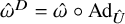 $\hat \omega ^D = \hat \omega \circ \mathrm {Ad}_{\hat U}$
are
$\hat \omega ^D = \hat \omega \circ \mathrm {Ad}_{\hat U}$
are
 $\hat \rho $
-locally comparable since
$\hat \rho $
-locally comparable since
 $\hat U \in \hat {\mathcal A}^{\mathrm {al}}$
and
$\hat U \in \hat {\mathcal A}^{\mathrm {al}}$
and ![]() is a
is a
 $0$
-chain of
$0$
-chain of
 $\hat {\mathcal A}$
. The state
$\hat {\mathcal A}$
. The state
 $\hat \omega = \omega \hat \otimes \omega '$
is Q-symmetric since
$\hat \omega = \omega \hat \otimes \omega '$
is Q-symmetric since
 $\omega $
is symmetric invertible. Moreover,
$\omega $
is symmetric invertible. Moreover,
 $\hat \omega ^D$
is Q-symmetric as well by Proposition 3.29. Thus
$\hat \omega ^D$
is Q-symmetric as well by Proposition 3.29. Thus
 $\mathcal I(\omega ) = \mathcal N_{\rho ^Q}(\hat \omega , \hat \omega ^D) \in \mathbb Z$
by Theorem 2.5(ii).
$\mathcal I(\omega ) = \mathcal N_{\rho ^Q}(\hat \omega , \hat \omega ^D) \in \mathbb Z$
by Theorem 2.5(ii).
(ii) This follows as in the proof of Proposition 3.23
(iii) Let
 $\tilde \omega $
be Q-equivalent to
$\tilde \omega $
be Q-equivalent to
 $\omega $
. Let
$\omega $
. Let
 $\beta $
be a Q-preserving LGA on
$\beta $
be a Q-preserving LGA on
 ${\mathcal A}$
such that
${\mathcal A}$
such that
 $\tilde \omega = \omega \circ \beta $
. Since
$\tilde \omega = \omega \circ \beta $
. Since
 $\omega $
is invertible, let
$\omega $
is invertible, let
 $ \omega '$
be its inverse. One has
$ \omega '$
be its inverse. One has
 $\omega \hat \otimes \omega ' = \hat \omega _0 \circ \hat \alpha $
with an
$\omega \hat \otimes \omega ' = \hat \omega _0 \circ \hat \alpha $
with an
 $LGA \hat \alpha $
and a pure product state
$LGA \hat \alpha $
and a pure product state
 $\hat \omega _0$
on
$\hat \omega _0$
on
 $\hat {\mathcal A}$
. Thus we have
$\hat {\mathcal A}$
. Thus we have
Thus
 $\tilde \omega $
is invertible. Moreover it is Q-symmetric and since
$\tilde \omega $
is invertible. Moreover it is Q-symmetric and since
 $\hat \omega $
is symmetric invertible then
$\hat \omega $
is symmetric invertible then
 $ \omega '$
is
$ \omega '$
is
 $Q'$
-symmetric. Thus
$Q'$
-symmetric. Thus
 $\tilde \omega $
is symmetric invertible, so that
$\tilde \omega $
is symmetric invertible, so that
 $\mathcal I(\tilde \omega )$
is well defined. The invariance of the index
$\mathcal I(\tilde \omega )$
is well defined. The invariance of the index
 $\mathcal I(\tilde \omega ) = \mathcal I(\omega )$
follows from Theorem 2.5(iv) on
$\mathcal I(\tilde \omega ) = \mathcal I(\omega )$
follows from Theorem 2.5(iv) on
 $\hat {\mathcal A}$
and goes along the same lines of the proof of Proposition 3.23 but on
$\hat {\mathcal A}$
and goes along the same lines of the proof of Proposition 3.23 but on
 $\hat {\mathcal A}$
.
$\hat {\mathcal A}$
.
(iv) If
 $\omega _1$
and
$\omega _1$
and
 $\omega _2$
are symmetric invertible with inverses
$\omega _2$
are symmetric invertible with inverses
 $ \omega ^{\prime }_1$
and
$ \omega ^{\prime }_1$
and
 $ \omega ^{\prime }_2$
, then
$ \omega ^{\prime }_2$
, then
 $\omega _1 \hat \otimes \omega _2$
is symmetric invertible on
$\omega _1 \hat \otimes \omega _2$
is symmetric invertible on
 ${\mathcal A}^1\hat \otimes {\mathcal A}^2$
with inverse
${\mathcal A}^1\hat \otimes {\mathcal A}^2$
with inverse
 $ \omega ^{\prime }_1\hat \otimes \omega ^{\prime }_2$
. The defect state construction factors on each algebra. In particular, up to the reshuffling
$ \omega ^{\prime }_1\hat \otimes \omega ^{\prime }_2$
. The defect state construction factors on each algebra. In particular, up to the reshuffling
 $$ \begin{align*}{\mathcal A}^1 \hat\otimes {\mathcal A}^2 \hat \otimes ({\mathcal A}^1)' \hat \otimes ({\mathcal A}^2)' \cong {\mathcal A}^1 \hat\otimes ({\mathcal A}^1)' \hat \otimes {\mathcal A}^2 \hat \otimes ({\mathcal A}^2)' = \hat {\mathcal A}^1 \hat \otimes \hat {\mathcal A}^2, \end{align*} $$
one has
 $(\hat \omega _1 \hat \otimes \hat \omega _2)^D = (\hat \omega _1)^D \hat \otimes (\hat \omega _2)^D$
so that, by Theorem 2.5(viii),
$(\hat \omega _1 \hat \otimes \hat \omega _2)^D = (\hat \omega _1)^D \hat \otimes (\hat \omega _2)^D$
so that, by Theorem 2.5(viii),
 $$ \begin{align*} \mathcal I(\omega_1 \hat\otimes \omega_2) &= \mathcal N_{\hat \rho^{Q_1}\hat\otimes \hat \rho^{Q_2}}(\omega_1 \hat\otimes \omega_2, (\hat \omega_1)^D \hat \otimes (\hat \omega_2)^D) \cr &= \mathcal N_{\hat \rho^{Q_1}}(\omega_1, (\hat \omega_1)^D) + \mathcal N_{\hat \rho^{Q_2}}(\omega_2, (\hat \omega_2)^D) \cr &= \mathcal I(\omega_1)+\mathcal I(\omega_2). \end{align*} $$
(v) This part is an immediate consequence of the quasi-free case, see Theorem 4.3 and Proposition Proposition 4.4 below.
Remark 3.33. One may wonder if the abstract index could also find some relevance for the fractional quantum Hall effect. We believe that it may be the case in following situation, which is similar to the quantization argument in [Reference Bachmann, Corbelli, Fraas and Ogata11]: Even if the initial state is not invertible, it may be that the flux insertion operation becomes inner after q units of quantum flux have been inserted. If this is the case, the arguments above yield a fractional Hall conductance of the form
 $\frac {n}{q}$
. It should be noted that in such a framework there is no prediction about the possible fractions one may obtain, see [Reference Fröhlich and Zee27].
$\frac {n}{q}$
. It should be noted that in such a framework there is no prediction about the possible fractions one may obtain, see [Reference Fröhlich and Zee27].
4 Quasi-free fermions and invertibility
We now return to the discussion at the beginning of Section 3.4 and we turn to the relation between the index of a pair of projections from Theorem 2.12 and the many-body index for the quantum Hall effect from Theorem 3.31, when applied to quasi-free states. We shall show that the two indices coincide when they are simultaneously well-defined.
Let
 $\mathcal H = \ell ^2(\mathbb Z^2)$
(for simplicity, we ignore spin here) and let P be the Fermi projection associated to some gapped local Hamiltonian H. Typically, we assume
$\mathcal H = \ell ^2(\mathbb Z^2)$
(for simplicity, we ignore spin here) and let P be the Fermi projection associated to some gapped local Hamiltonian H. Typically, we assume
 $$ \begin{align}|H_{x,y}|:= |\langle \delta_x, H \delta_y\rangle | \leq C {\mathrm e}^{-\mu|x-y|}, \end{align} $$
and the kernel of P has the same property whenever the Fermi energy lies in a gap. Consider the quasi-free state
 $\omega _P$
on
$\omega _P$
on
 ${\mathcal A}=\mathrm {CAR}(\mathcal H)$
, see (20) above. We first recall
${\mathcal A}=\mathrm {CAR}(\mathcal H)$
, see (20) above. We first recall
Proposition 4.1 [Reference Bachmann, Bols and Rahnama10, Proposition 2.5].
Assume H is translation-invariant on
 $\mathcal H$
and consider the associated Chern number
$\mathcal H$
and consider the associated Chern number
 $c(P)$
for the Fermi projection. If
$c(P)$
for the Fermi projection. If
 $c(P)=0$
then
$c(P)=0$
then
 $\omega _P$
is stably SRE.
$\omega _P$
is stably SRE.
Note that the assumption there is about time-reversal invariance, but the argument (in [Reference Bachmann, Bols and Rahnama10, Appendix B]) goes though the consequence thereof, which is that the Chern number vanishes.
Conversely, if a quasi-free state is stably SRE and the deformation is a family of quasi-free states, then the smooth path of states yields a smooth deformation of the bundle to a trivial bundle and so the Chern number must vanish.
Translation invariance is not expected to be relevant for this question. Indeed, [Reference Chung and Shapiro23] proves that if P and Q have the same Chern number and both satisfy a certain nontriviality assumption ([Reference Chung and Shapiro23, Definition 1.2]), then there exists a path of local unitaries
 $[0,1]\ni t\mapsto U_t$
with
$[0,1]\ni t\mapsto U_t$
with ![]() such that
such that
 $Q=U_1^\ast P U_1$
, that is, P and Q are homotopic within the space of local projections.
$Q=U_1^\ast P U_1$
, that is, P and Q are homotopic within the space of local projections.
Now suppose P has zero Chern number. By the same result, we can connect P to a projection Q that is diagonal in space (and hence also has zero Chern number). By lifting
 $t\mapsto U_t$
to an LGA, this yields a continuous path from
$t\mapsto U_t$
to an LGA, this yields a continuous path from
 $\omega _P$
to
$\omega _P$
to
 $\omega _Q$
(a product state), and therefore shows that
$\omega _Q$
(a product state), and therefore shows that
 $\omega _P$
is an SRE state.
$\omega _P$
is an SRE state.
The problem with this argument is that the notion of locality used in [Reference Chung and Shapiro23] is a far cry from (38): there, P is local iff
 $[P,L]\in \mathcal {K}$
, where L is the Laughlin unitary
$[P,L]\in \mathcal {K}$
, where L is the Laughlin unitary
 $L\equiv \exp \left (\operatorname {i}\arg \left (X_1+\operatorname {i} X_2\right )\right )$
. Bridging this gap would require formulating an analogous notion of locality in the many-body setting (and proving a Lieb–Robinson bound for it). Since this line of study is rather tangential to the present paper we do not pursue it further here and instead merely phrase a
$L\equiv \exp \left (\operatorname {i}\arg \left (X_1+\operatorname {i} X_2\right )\right )$
. Bridging this gap would require formulating an analogous notion of locality in the many-body setting (and proving a Lieb–Robinson bound for it). Since this line of study is rather tangential to the present paper we do not pursue it further here and instead merely phrase a
Conjecture 4.2. Let H be a gapped Hamiltonian obeying (38) for which the Fermi projection P has a well-defined topological index
 $c(P)$
. Then
$c(P)$
. Then
 $c(P)=0$
if and only if
$c(P)=0$
if and only if
 $\omega _P$
is stably SRE.
$\omega _P$
is stably SRE.
Note that the ‘topological index’
 $c(P)$
is, strictly speaking, a ‘Chern number’ only in the periodic setting, but we continue to use the same symbol for it.
$c(P)$
is, strictly speaking, a ‘Chern number’ only in the periodic setting, but we continue to use the same symbol for it.
We return to the notion of invertibility in the quasi-free setting. Let
 $\mathcal H \hat \oplus \mathcal H$
be the external direct sum and consider the projection
$\mathcal H \hat \oplus \mathcal H$
be the external direct sum and consider the projection
 $P\hat \oplus P^\perp $
, where
$P\hat \oplus P^\perp $
, where ![]() . One then has
. One then has
 $c(P\hat \oplus P^\perp ) = c(P)+c(P^\perp )=0$
. It follows that, in the translation-invariant setting, the state
$c(P\hat \oplus P^\perp ) = c(P)+c(P^\perp )=0$
. It follows that, in the translation-invariant setting, the state
 $\omega _{P\hat \oplus P^\perp } = \omega _P \hat \otimes \omega _{P^\perp }$
is stably-SRE. Consequently, the quasi-free state
$\omega _{P\hat \oplus P^\perp } = \omega _P \hat \otimes \omega _{P^\perp }$
is stably-SRE. Consequently, the quasi-free state
 $\omega _P$
is invertible. In particular, we can associate to it the many-body index
$\omega _P$
is invertible. In particular, we can associate to it the many-body index
 ${\mathcal I}(\omega _P)$
.
${\mathcal I}(\omega _P)$
.
We use the independence of the index on the parent Hamiltonian provided by Theorem 3.31(ii) to choose
 $H\hat \oplus (-H)$
as parent Hamiltonian to
$H\hat \oplus (-H)$
as parent Hamiltonian to
 $P\hat \oplus P^\perp $
. Note that this direct sum structure is not what would arise from the general construction presented in Lemma 3.11 because the automorphism mapping
$P\hat \oplus P^\perp $
. Note that this direct sum structure is not what would arise from the general construction presented in Lemma 3.11 because the automorphism mapping
 $\omega _{P\hat \oplus P^\perp }$
to a product state would in general mix the two layers. Now if the parent Hamiltonian is a direct sum, then the flux insertion unitary similarly factorizes as
$\omega _{P\hat \oplus P^\perp }$
to a product state would in general mix the two layers. Now if the parent Hamiltonian is a direct sum, then the flux insertion unitary similarly factorizes as
 $U^{\mathrm {qa}}_{\phi _1,\phi _2} \hat \oplus U^{\mathrm {qa}}_{\phi _1,\phi _2}$
. Here
$U^{\mathrm {qa}}_{\phi _1,\phi _2} \hat \oplus U^{\mathrm {qa}}_{\phi _1,\phi _2}$
. Here
 $U^{\mathrm {qa}}_{\phi _1,\phi _2}$
is the flux-insertion unitary given by
$U^{\mathrm {qa}}_{\phi _1,\phi _2}$
is the flux-insertion unitary given by
where
 $K_\phi =\chi _{\mathrm {left}} K^\uparrow _\phi \chi _{\mathrm {left}}$
and
$K_\phi =\chi _{\mathrm {left}} K^\uparrow _\phi \chi _{\mathrm {left}}$
and
 $K^\uparrow _\phi = -\operatorname {i}[\partial P^\uparrow _\phi , P^\uparrow _\phi ]$
is the Kato generator of the family of projections
$K^\uparrow _\phi = -\operatorname {i}[\partial P^\uparrow _\phi , P^\uparrow _\phi ]$
is the Kato generator of the family of projections
 $P^\uparrow _\phi = {\mathrm e}^{\operatorname {i} \phi \chi _\uparrow }P{\mathrm e}^{-\operatorname {i} \phi \chi _\uparrow }$
.
$P^\uparrow _\phi = {\mathrm e}^{\operatorname {i} \phi \chi _\uparrow }P{\mathrm e}^{-\operatorname {i} \phi \chi _\uparrow }$
.
 $\chi _\uparrow $
and
$\chi _\uparrow $
and
 $\chi _{\mathrm {left}}$
are the respective projections to the upper and left half-planes. See [Reference Bachmann, Bols and Rahnama10, Sec 5.1] for more details.
$\chi _{\mathrm {left}}$
are the respective projections to the upper and left half-planes. See [Reference Bachmann, Bols and Rahnama10, Sec 5.1] for more details.
As a result, the defect state is again a quasi-free state, corresponding to a projection
 $P^{\mathrm {qa}}_{2\pi }\hat \oplus (P^{\mathrm {qa}}_{2\pi })^\perp $
, where
$P^{\mathrm {qa}}_{2\pi }\hat \oplus (P^{\mathrm {qa}}_{2\pi })^\perp $
, where
 $P^{\mathrm {qa}}_{2\pi } = U^{\mathrm {qa}}_{0,2\pi } P (U^{\mathrm {qa}}_{0,2\pi })^{*}$
. With this, the construction in the proof of Theorem 2.12 completely factorizes. However, in the final step of the proof when one computes the index, the charge automorphism
$P^{\mathrm {qa}}_{2\pi } = U^{\mathrm {qa}}_{0,2\pi } P (U^{\mathrm {qa}}_{0,2\pi })^{*}$
. With this, the construction in the proof of Theorem 2.12 completely factorizes. However, in the final step of the proof when one computes the index, the charge automorphism
 $\rho $
must be taken with
$\rho $
must be taken with ![]() rather than
rather than ![]() , see the definition in (37) and the discussion before it. Hence
, see the definition in (37) and the discussion before it. Hence
 $\delta ^\rho $
acts trivially on the second factor and we conclude
$\delta ^\rho $
acts trivially on the second factor and we conclude
Theorem 4.3. If the difference
 $P-P^{\mathrm {qa}}_{2\pi }$
is trace class then
$P-P^{\mathrm {qa}}_{2\pi }$
is trace class then
 $$ \begin{align*}\mathcal I(\omega_P) = \mathrm{index}(P, P^{\mathrm{qa}}_{2\pi}). \end{align*} $$
One may wonder when
 $P-P^{\mathrm {qa}}_{2\pi }$
is trace class, so that the index on the right-hand side is well defined. A typical case is given by a local Hamiltonian as described above with Fermi level in a spectral gapFootnote
1
and Proposition 4.4 below. Consider then the instantaneous Fermi projection
$P-P^{\mathrm {qa}}_{2\pi }$
is trace class, so that the index on the right-hand side is well defined. A typical case is given by a local Hamiltonian as described above with Fermi level in a spectral gapFootnote
1
and Proposition 4.4 below. Consider then the instantaneous Fermi projection
 $P^{\mu }_\phi = \chi _{(-\infty , \mu ]}({H}_{\phi })$
for the Hamiltonians
$P^{\mu }_\phi = \chi _{(-\infty , \mu ]}({H}_{\phi })$
for the Hamiltonians
 ${H}_{\phi }$
defined by
${H}_{\phi }$
defined by
 $$ \begin{align} {H}_{\phi}(x, i; y, j) = \begin{cases} \mathrm{e}^{\mathrm{i} \phi \, \mathrm{sgn}( x_2 - y_2 )} {H}(x, i; y, j) & \text{if } x_1, y_1 \leq 0 \\ {H}(x, i; y, j) & \text{otherwise} \end{cases} \end{align} $$
Notice that, by construction,
 $H_{2\pi }=H_0$
so that
$H_{2\pi }=H_0$
so that
 $H_{2\pi }$
is gapped around
$H_{2\pi }$
is gapped around
 $\mu $
as well, and moreover
$\mu $
as well, and moreover
 $P^{\mu }_{2\pi } = P^\mu _0 = P$
.
$P^{\mu }_{2\pi } = P^\mu _0 = P$
.
Proposition 4.4 [Reference Bachmann, Bols and Rahnama10, Proof of Prop. 5.1].
Let
 $\mu $
be in the spectral gap of
$\mu $
be in the spectral gap of
 $H_0$
and such that all eigenvalues crossings of
$H_0$
and such that all eigenvalues crossings of
 $\phi \mapsto {H}_{\phi }$
across
$\phi \mapsto {H}_{\phi }$
across
 $\mu $
are simple. Then for all
$\mu $
are simple. Then for all
 $\phi $
the difference
$\phi $
the difference
 $P^{\mathrm {qa}}_{\phi } - P^{\mu }_{\phi }$
is trace class and
$P^{\mathrm {qa}}_{\phi } - P^{\mu }_{\phi }$
is trace class and
 $$ \begin{align*} \mathrm{SF}_{\mu}( [0, 2\pi] \ni \phi \mapsto H_{\phi} ) = \mathrm{Tr} (P^{\mathrm{qa}}_{2\pi} - P^{\mu}_{2\pi}). \end{align*} $$
We recall that the spectral flow counts the signed number of eigenvalue crossings with the fiducial line at
 $\mu $
. See for example [Reference De Nittis and Schulz-Baldes24] for a detailed study of spectral flow in the single-particle and discrete setting for Quantum Hall effect.
$\mu $
. See for example [Reference De Nittis and Schulz-Baldes24] for a detailed study of spectral flow in the single-particle and discrete setting for Quantum Hall effect.
Summarizing, under the hypothesis of Proposition 4.4, one has various single-particle interpretations of the index,
 $$ \begin{align*}\mathcal I(\omega_P) = \mathrm{index}(P^{\mathrm{qa}}_{2\pi},P^\mu_{2\pi}) = \mathrm{Tr}(P^{\mathrm{qa}}_{2\pi}-P^\mu_{2\pi})= \mathrm{SF}_{\mu}( [0, 2\pi] \ni \phi \mapsto {h}_{\phi} ) \end{align*} $$
which ultimately appears as a many-body version of spectral flow induced by magnetic flux insertion.
4.1 Beyond quasi-free states
We now have a complete picture of the relationship between the many-body index of a pair of pure states, the index of a pair of projections, the spectral flow associated with flux insertion and the spectral flow in a noninteracting picture. We point out that the stability of the many-body index and many-body perturbation theory allow one to go beyond the free setting. The proposition below is phrased in a translation-invariant setting to be able to use Proposition 4.1. This assumption can be dropped if Conjecture 4.2 is true.
Proposition 4.5. Let
 $H_\lambda =H_0+\lambda V$
where H and V are two Q-preserving
$H_\lambda =H_0+\lambda V$
where H and V are two Q-preserving
 $0$
-chains in
$0$
-chains in
 ${\mathcal A}$
. Assume that for all
${\mathcal A}$
. Assume that for all
 $\lambda \in [0,1]$
,
$\lambda \in [0,1]$
,
 $H_\lambda $
has a locally unique gapped ground state
$H_\lambda $
has a locally unique gapped ground state
 $\omega _\lambda $
, and that
$\omega _\lambda $
, and that
 $\omega _0$
is a quasi-free translation-invariant state. Then
$\omega _0$
is a quasi-free translation-invariant state. Then
 $\omega _{1}$
is invertible and
$\omega _{1}$
is invertible and
 $\mathcal I(\omega _{1})=\mathcal I (\omega _0)$
.
$\mathcal I(\omega _{1})=\mathcal I (\omega _0)$
.
Note that a locally unique gapped ground state is necessarily pure, see [Reference Tasaki45, Theorem A.3].
Proof. Since
 $H_\lambda $
has a uniform gapped ground state then the spectral flow [Reference Bachmann, Michalakis, Nachtergaele and Sims16], generated by a
$H_\lambda $
has a uniform gapped ground state then the spectral flow [Reference Bachmann, Michalakis, Nachtergaele and Sims16], generated by a
 $0$
-chain
$0$
-chain
 $K_\lambda $
, is such that
$K_\lambda $
, is such that
 $\omega _{\lambda }= \omega _0\circ \alpha _{0\to \lambda }^K$
. Then since
$\omega _{\lambda }= \omega _0\circ \alpha _{0\to \lambda }^K$
. Then since
 $\omega _0$
is quasi-free then it admits an inverse
$\omega _0$
is quasi-free then it admits an inverse
 $\omega ^{\prime }_0$
on
$\omega ^{\prime }_0$
on
 ${\mathcal A}'$
. Now,
${\mathcal A}'$
. Now,
and since
 $\omega _0 \hat \otimes \omega ^{\prime }_0$
is stably SRE, this shows that
$\omega _0 \hat \otimes \omega ^{\prime }_0$
is stably SRE, this shows that
 $\omega _1$
is invertible. Finally, since
$\omega _1$
is invertible. Finally, since
 $H_\lambda $
is Q-preserving, then
$H_\lambda $
is Q-preserving, then
 $\alpha ^K$
is Q-preserving. Thus
$\alpha ^K$
is Q-preserving. Thus
 $\omega _1$
is Q-equivalent to
$\omega _1$
is Q-equivalent to
 $\omega _0$
and so
$\omega _0$
and so
 $\mathcal I(\omega _{1})=\mathcal I (\omega _0)$
by Theorem 3.31(iii).
$\mathcal I(\omega _{1})=\mathcal I (\omega _0)$
by Theorem 3.31(iii).
Acknowledgments
We are indebted to Alex Bols, Christopher Bourne, Gian Michele Graf and Anna Mazhar for stimulating discussions. JS is indebted to the CEREMADE at Université Paris-Dauphine – PSL, as well as the Institute for Theoretical Physics at ETH for hospitality in the summer of 2025.
Competing interests
The authors have no competing interest to declare.
Financial support
JS is supported in part by NSF grant DMS-2510207. SB is supported by NSERC of Canada.


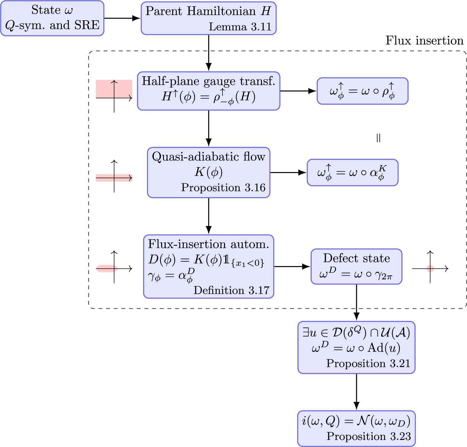


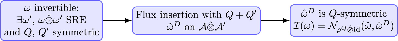

 Open access