





1 Introduction
Active particles are entities that use internal mechanisms to put energy into the surrounding environment to drive their own directed motion. There are many different types of active particles in biological systems, including simple microorganisms such as bacteria, algae or sperm cells, as well as higher organisms such as humans, mammals, birds and fish. Self-propelled microorganisms in fluids are generally called microswimmers [Reference Elgeti, Winkler and Gompper8]. In addition, active particles can be viewed as artificial self-propelled microswimmers [Reference Bechinger, Di Leonardo, Löwen, Reichhardt and Volpe3, Reference Ramaswamy15]. Theoretical and experimental investigations of these systems have grown considerably in recent years, with foundational reviews covering the hydrodynamics of swimming microorganisms [Reference Lauga and Powers10], active particles in complex and crowded environments [Reference Bechinger, Di Leonardo, Löwen, Reichhardt and Volpe3] and magnetically driven microbots and nanobots [Reference Zhou, Mayorga-Martinez, Pan’e, Zhang and Pumera21]. Microswimmers consistently interact with a surrounding fluid flow in a variety of conditions. For example, microswimmers commonly experience unidirectional flows in confined channels, such as microorganisms in laminar flow through a porous matrix, pathogens in the blood stream, sperm cells swimming in fallopian tubes [Reference Bhattacharjee and Datta4, Reference Levy, Hill, Forest and Grotberg11, Reference Riffell and Zimmer16] and microrobots used for targeted drug delivery applications [Reference Nguyen14].
Understanding the dynamics of active particles in confined geometries has significant applications in various fields, including biomedicine, environmental sciences [Reference Al Harraq, Bello and Bharti2] and the food industry [Reference Szpicer, Bińkowska, Wojtasik-Kalinowska, Salih and Półtorak18]. It is also essential to design artificial microswimmers for biomedical applications such as cell manipulation, targeted drug delivery and cargo transport [Reference Akcayoglu, Sahin, Canpolat and Akilli1]. Furthermore, it can help improve the design of industrial and biomedical microfluidic devices intended to focus, sort and/or filter microorganisms in fluid suspensions [Reference Sajeesh and Sen17].
Various models for the dynamics of microswimmers in Poiseuille flow have been studied. Examples include a study of chaotic dynamics of point-like, spherical particles [Reference Chacón5], an examination of swinging motion of active deformable particles [Reference Tarama19], the observation of upstream swimming [Reference Mathijssen, Shendruk, Yeomans and Doostmohammadi13] and modelling the dynamics of microswimmers in pressure-driven flow in a weakly viscoelastic fluid [Reference Choudhary and Stark6]. While there is a significant quantity of work that builds on the squirmer model introduced by Lighthill [Reference Lighthill12], this article is concerned with the core components of these simpler models of active particle motion.
Zöttl and Stark studied the dynamics of a point-like spherical microswimmer in a cylindrical Poiseuille flow [Reference Zöttl and Stark22]. They identified two basic swimming states, an upstream oriented swinging motion around the centreline and tumbling similar to the passive particles. They demonstrated that the swimmer performs either periodic swinging or periodic tumbling motion in a cylindrical microchannel. The dynamics of a prolate spheroidal microswimmer in Poiseuille flow through cylindrical and elliptical pipes was subsequently examined [Reference Zöttl and Stark23]. Although their results only illustrate quasi-periodic motion in the case of elliptical pipes, it is straightforward to generate examples of chaotic trajectories in this case. More complex variations of this model have also been explored, for example, including effects of gyrotactic reorientation, spheroidal particle/swimmer shape and rotational noise/diffusivity [Reference Croze, Sardina, Ahmed, Bees and Brandt7].
Valani et al. [Reference Valani, Harding and Stokes20] applied the Zöttl and Stark model to study the dynamics of a point-like active particle suspended in fluid flow through a straight rectangular duct. They derived a constant of motion for general unidirectional fluid flow and applied the model using a polynomial approximation of a Poiseuille flow through a square cross-section. In addition to the swinging, trapping, tumbling and wandering motions identified previously, they observed chaotic orbits. They further investigated the transition to chaotic orbits through Poincaré maps and Lyapunov exponents, which revealed sticky chaotic tumbling trajectories near periodic states. Recently, Harding et al. [Reference Harding, Valani and Stokes9] revealed a general Hamiltonian structure in the broader class of point-like active particle models for both spherical and spheroidal particle shapes.
In this paper, we study the dynamics of spherical active particle motion suspended in a cubic Poiseuille field inspired by steady viscous fluid flow through an equilateral triangular channel. Using the general Hamiltonian formulation of Harding et al. [Reference Harding, Valani and Stokes9], we describe the equations of motion for a spherical particle in this specific geometry. This geometric configuration presents a unique opportunity to understand the behaviour of microswimmers in a setting where the Poiseuille flow is described (exactly) by a cubic polynomial. This velocity field stands in contrast to other common geometries, such as rectangular ducts that require series solutions. This leads to a relatively straightforward closed-form description of the Hamiltonian structure and corresponding equations of motion. It also facilitates efficient and precise simulations, for example, by avoiding truncation errors inherent in an approximate series solution for Poiseuille flow. Simultaneously, the cubic velocity field provides slightly more complexity than the quadratic Poiseuille flow that occurs through circular and elliptical pipes. The equilateral triangular geometry also possesses the symmetry group $D_3$
, the smallest non-Abelian group, and provides an opportunity to examine whether there exist any unique orbits associated with such symmetry. Using the tools and classification criteria of recent studies [Reference Harding, Valani and Stokes9, Reference Valani, Harding and Stokes20], we examine the trajectories of active particle dynamics under a wide variety of initial conditions and parameter values. This work generally adds prior insights into the dynamics of active particles in confined environments.
$D_3$
, the smallest non-Abelian group, and provides an opportunity to examine whether there exist any unique orbits associated with such symmetry. Using the tools and classification criteria of recent studies [Reference Harding, Valani and Stokes9, Reference Valani, Harding and Stokes20], we examine the trajectories of active particle dynamics under a wide variety of initial conditions and parameter values. This work generally adds prior insights into the dynamics of active particles in confined environments.
2 Mathematical model
We use the formulation of Harding et al. [Reference Harding, Valani and Stokes9] describing the dynamics of active particle motion in Poiseuille flow through a straight duct aligned with the z-axis. Following that work, we assume there is a pressure-driven flow through the duct that is steady, incompressible, fully developed in the (positive) z-direction and satisfies a no slip boundary condition at the channel walls. The velocity field is generically described by $w(x,y)\mathbf {k}$
. Further, we assume there are no external body forces influencing the physics.
$w(x,y)\mathbf {k}$
. Further, we assume there are no external body forces influencing the physics.
Consider a spherical point-like active particle model of a microswimmer suspended in the fluid flow. The point-like assumption implies that we neglect any effect that the microswimmer may have on the fluid flow. Let $\mathbf {r}(t)=x(t)\hat {\mathbf {i}}+y(t)\hat {\mathbf {j}}+z(t)\hat {\mathbf {k}}$
describe the location of the microswimmer (specifically its centre) at each time
$\mathbf {r}(t)=x(t)\hat {\mathbf {i}}+y(t)\hat {\mathbf {j}}+z(t)\hat {\mathbf {k}}$
describe the location of the microswimmer (specifically its centre) at each time $t\geq 0$
. It will be assumed that, in addition to being carried by the flow, the microswimmer propels itself with a constant intrinsic swimming speed
$t\geq 0$
. It will be assumed that, in addition to being carried by the flow, the microswimmer propels itself with a constant intrinsic swimming speed $v_{0}$
in the direction of its orientation vector
$v_{0}$
in the direction of its orientation vector $\hat {\mathbf {e}}(t)=e_{x}(t)\hat {\mathbf {i}}+e_{y}(t)\hat {\mathbf {j}}+e_{z}(t)\hat {\mathbf {k}}$
. The microswimmer is rotated as a result of the gradient in the fluid velocity field. This shear induced rotation is assumed to be the primary/sole mechanism which modifies the orientation vector. The equations of motion for the active particles are given by
$\hat {\mathbf {e}}(t)=e_{x}(t)\hat {\mathbf {i}}+e_{y}(t)\hat {\mathbf {j}}+e_{z}(t)\hat {\mathbf {k}}$
. The microswimmer is rotated as a result of the gradient in the fluid velocity field. This shear induced rotation is assumed to be the primary/sole mechanism which modifies the orientation vector. The equations of motion for the active particles are given by
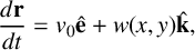 $$ \begin{align} \frac{d\mathbf{r}}{dt}&=v_{0}\hat{\mathbf{e}}+w(x,y)\hat{\mathbf{k}}, \end{align} $$
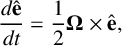 $$ \begin{align} \frac{d\hat{\mathbf{e}}}{dt}&=\frac{1}{2}\boldsymbol{\Omega} \times \hat{\mathbf{e}}, \end{align} $$
where $\boldsymbol {\Omega }= \nabla \times w(x,y)\hat {\mathbf {k}}$
is the vorticity of the fluid flow. Here, (2.1a) describes the microswimmer’s translational motion as the sum of its intrinsic velocity
$\boldsymbol {\Omega }= \nabla \times w(x,y)\hat {\mathbf {k}}$
is the vorticity of the fluid flow. Here, (2.1a) describes the microswimmer’s translational motion as the sum of its intrinsic velocity $v_{0}\hat {\mathbf {e}}$
and the local velocity of the background fluid flow
$v_{0}\hat {\mathbf {e}}$
and the local velocity of the background fluid flow $w(x,y)\hat {\mathbf {k}}$
, whereas (2.1b) describes how the orientation of the microswimmer changes due to the local fluid vorticity.
$w(x,y)\hat {\mathbf {k}}$
, whereas (2.1b) describes how the orientation of the microswimmer changes due to the local fluid vorticity.
Herein, we set $v_0=1$
(without loss of generality), which is equivalent to a partial non-dimensionalization in which we introduce the dimensionless flow field
$v_0=1$
(without loss of generality), which is equivalent to a partial non-dimensionalization in which we introduce the dimensionless flow field $\bar {w}(x,y)=w(x,y)/v_{0}$
, and use the rescaled time
$\bar {w}(x,y)=w(x,y)/v_{0}$
, and use the rescaled time $\bar {t}=v_0 t$
and vorticity
$\bar {t}=v_0 t$
and vorticity $\bar {\boldsymbol {\Omega }}=\boldsymbol {\Omega }/v_{0}$
. The equations of motion are then
$\bar {\boldsymbol {\Omega }}=\boldsymbol {\Omega }/v_{0}$
. The equations of motion are then
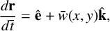 $$ \begin{align} \frac{d\mathbf{r}}{d\bar{t}}&=\hat{\mathbf{e}}+\bar{w}(x,y)\hat{\mathbf{k}},\end{align} $$
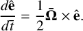 $$ \begin{align} \frac{d\hat{\mathbf{e}}}{d\bar{t}}&=\frac{1}{2}\bar{\boldsymbol{\Omega}} \times \hat{\mathbf{e}}.\end{align} $$
The magnitude of $\bar {w}$
can be thought of as a parameter which controls the flow speed relative to the swimmer speed. Changes in the spatial scaling can be absorbed into the time scaling and have no material effect on the dynamics.
$\bar {w}$
can be thought of as a parameter which controls the flow speed relative to the swimmer speed. Changes in the spatial scaling can be absorbed into the time scaling and have no material effect on the dynamics.
We briefly summarize the derivation of a Hamiltonian formulation of this system [Reference Harding, Valani and Stokes9]. Expressed in component form, (2.2) is a system of six nonlinear ordinary differential equations:
 $$ \begin{align} \dot{x} &= e_{x}, \end{align} $$
 $$ \begin{align} \dot{y} &= e_{y}, \end{align} $$
 $$ \begin{align} \dot{z} &= e_{z} + \bar{w}(x,y), \end{align} $$
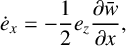 $$ \begin{align} \dot{e}_x &= -\frac{1}{2} e_{z} \frac{\partial \bar{w}}{\partial x}, \end{align} $$
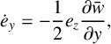 $$ \begin{align} \dot{e}_y &= -\frac{1}{2} e_{z} \frac{\partial \bar{w}}{\partial y}, \end{align} $$
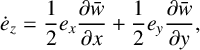 $$ \begin{align} \dot{e}_z &= \frac{1}{2} e_{x} \frac{\partial \bar{w}}{\partial x} + \frac{1}{2} e_{y} \frac{\partial \bar{w}}{\partial y},\end{align} $$
where $\dot {x}$
is shorthand for
$\dot {x}$
is shorthand for $dx/d\bar {t}$
. The z variable decouples and the dynamics are described by the five remaining differential equations. The effective dimension of the dynamical system is further reduced by identifying constants of motion (that is, quantities that remain constant throughout the system’s evolution). A trivial constant of motion for our system is given by
$dx/d\bar {t}$
. The z variable decouples and the dynamics are described by the five remaining differential equations. The effective dimension of the dynamical system is further reduced by identifying constants of motion (that is, quantities that remain constant throughout the system’s evolution). A trivial constant of motion for our system is given by
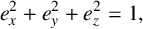 $$ \begin{align*} e_{x}^{2}+e_{y}^{2}+e_{z}^{2}=1, \end{align*} $$
since the orientation vector must maintain unit magnitude. An additional constant of motion, obtained by integrating (2.3f) after substitution using (2.3a) and (2.3b), is given by
 $$ \begin{align} c_0 = e_z-\tfrac{1}{2}\bar{w}(x,y). \end{align} $$
This can be substituted into (2.3d) and (2.3e) to produce a second-order system in terms of $x,y$
(noting
$x,y$
(noting $\dot {e}_x=\ddot {x}$
and
$\dot {e}_x=\ddot {x}$
and $\dot {e}_y=\ddot {y}$
). On inspection, one can deduce that the second-order equations are equivalent to a description of the motion of a point within the potential field
$\dot {e}_y=\ddot {y}$
). On inspection, one can deduce that the second-order equations are equivalent to a description of the motion of a point within the potential field
 $$ \begin{align*} V = \tfrac{1}{2}(c_0+\tfrac{1}{2}\bar{w}(x,y) )^2. \end{align*} $$
Consequently, our system admits the Hamiltonian
 $$ \begin{align} H=\tfrac{1}{2} (e_{x}^{2}+e_{y}^{2})+\tfrac{1}{2}(c_{0}+\tfrac{1}{2}\bar{w}(x,y))^2, \end{align} $$
where $e_x=\dot {x}$
and
$e_x=\dot {x}$
and $e_y=\dot {y}$
may be interpreted as momenta. Explicitly, the equations of motion (2.3a), (2.3b), (2.3d) and (2.3e) can be recovered from Hamilton’s equations:
$e_y=\dot {y}$
may be interpreted as momenta. Explicitly, the equations of motion (2.3a), (2.3b), (2.3d) and (2.3e) can be recovered from Hamilton’s equations:
 $$ \begin{align*} \dot{x}=\frac{\partial{H}}{\partial e_{x} },\quad \dot{y}=\frac{\partial{H}}{\partial e_{y} },\quad \dot{e}_x=-\frac{\partial{H}}{\partial x},\quad \dot{e}_y=-\frac{\partial{H}}{\partial y }, \end{align*} $$
in combination with (2.4). Observe that the Hamiltonian is equivalent to $\|\mathbf {e}\|^2/2$
and does not constitute an additional constant of motion of (2.3). Thus, we can conclude that the dynamics of the system are constrained to a manifold having (at most) three dimensions. The identification of the potential field, V, provides a mechanism to determine the region of the cross-section in which an orbit is confined. Specifically, having determined a
$\|\mathbf {e}\|^2/2$
and does not constitute an additional constant of motion of (2.3). Thus, we can conclude that the dynamics of the system are constrained to a manifold having (at most) three dimensions. The identification of the potential field, V, provides a mechanism to determine the region of the cross-section in which an orbit is confined. Specifically, having determined a $c_0$
from given initial conditions, then
$c_0$
from given initial conditions, then $x(t),y(t)$
is confined to the region satisfying
$x(t),y(t)$
is confined to the region satisfying $V\leq 1/2$
.
$V\leq 1/2$
.
Herein, we consider the above system in the specific case of the Poiseuille field obtained from a duct having an equilateral triangular cross-section with a side length L. Without loss of generality, we place one corner of the cross-section at the origin within the x–y plane and extend the bottom edge along the positive x-axis. The associated Poiseuille flow possesses a velocity directed parallel to the (positive) z-axis with magnitude described by
 $$ \begin{align} \bar{w}(x,y)=\frac{U}{N}y(y-\sqrt{3}x)(y+\sqrt{3}x-\sqrt{3}L), \end{align} $$
where $N=L^{3}/\sqrt {108}$
and U is the maximum velocity that is attained at the centroid
$N=L^{3}/\sqrt {108}$
and U is the maximum velocity that is attained at the centroid $(x,y)=(L/2,L/\sqrt {12})$
. It can be readily verified that the Laplacian of this field is constant,
$(x,y)=(L/2,L/\sqrt {12})$
. It can be readily verified that the Laplacian of this field is constant,
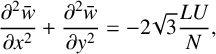 $$ \begin{align*}\frac{\partial^2 \bar{w}}{\partial x^2}+\frac{\partial^2 \bar{w}}{\partial y^2}=-2\sqrt{3}\frac{LU}{N},\end{align*} $$
implying that $-36\mu U/L^2$
is the pressure gradient required to drive the given flow for a fluid with viscosity
$-36\mu U/L^2$
is the pressure gradient required to drive the given flow for a fluid with viscosity $\mu $
. In addition, the net flux is
$\mu $
. In addition, the net flux is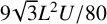 $9\sqrt {3}L^2U/80$
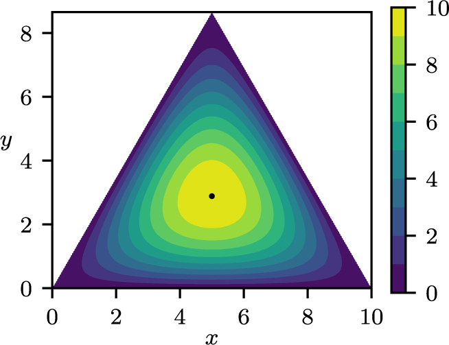
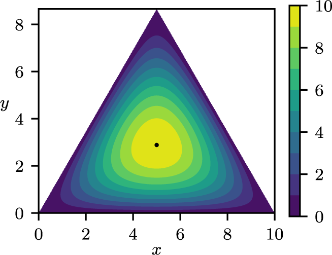
. Contours of (2.6) are shown in Figure 1.
$9\sqrt {3}L^2U/80$
. Contours of (2.6) are shown in Figure 1.
Velocity distribution of Poiseuille flow through an equilateral triangular duct. Here, we set the side length $L=10$
and the maximum velocity
$L=10$
and the maximum velocity $U=10$
, as is used for most examples throughout. The centroid is marked with a dot.
$U=10$
, as is used for most examples throughout. The centroid is marked with a dot.
Given this specific $\bar {w}$
, the equations of motion for an active particle, derived from the Hamiltonian (2.5), are
$\bar {w}$
, the equations of motion for an active particle, derived from the Hamiltonian (2.5), are
 $$ \begin{align} \dot{x}&=e_{x}, \end{align} $$
 $$ \begin{align} \dot{y}&=e_{y}, \end{align} $$
 $$ \begin{align} \dot{e}_x&=-\frac{3}{2}\frac{U}{N}y(L-2x)\left(c_{0}+\frac{U}{2N} (y^{3}-\sqrt{3}Ly^{2}-3x^{2}y+3Lxy)\right), \end{align} $$
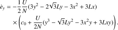 $$ \begin{align} \dot{e}_y&=-\frac{1}{2}\frac{U}{N} (3y^{2}-2\sqrt{3}Ly-3x^{2}+3Lx) \nonumber \\ &\quad \times \left(c_{0}+\frac{U}{2N} (y^{3}-\sqrt{3}Ly^{2}-3x^{2}y+3Lxy)\right). \end{align} $$
The value of $e_z$
can be recovered at any moment in time via
$e_z$
can be recovered at any moment in time via
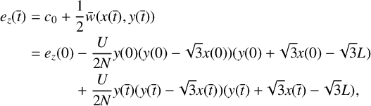 $$ \begin{align*} e_z(\bar{t}) &=c_0+\frac{1}{2}\bar{w}(x(\bar{t}),y(\bar{t})) \\ &=e_z(0)-\frac{U}{2N}y(0)(y(0)-\sqrt{3}x(0))(y(0)+\sqrt{3}x(0)-\sqrt{3}L) \\ &\phantom{{}=e_z(0)}+\frac{U}{2N}y(\bar{t})(y(\bar{t})-\sqrt{3}x(\bar{t}))(y(\bar{t})+\sqrt{3}x(\bar{t})-\sqrt{3}L) , \end{align*} $$
using $c_0$
determined from prescribed initial conditions
$c_0$
determined from prescribed initial conditions $x(0),y(0),\mathbf {e}(0)$
.
$x(0),y(0),\mathbf {e}(0)$
.
3 Equilibrium points and stability
An analysis of equilibrium points and their stability in a general setting (that is, with arbitrary $\bar {w}(x,y)$
) was conducted by Harding et al. [Reference Harding, Valani and Stokes9]. Here, we summarize the results in this specific case where
$\bar {w}(x,y)$
) was conducted by Harding et al. [Reference Harding, Valani and Stokes9]. Here, we summarize the results in this specific case where $\bar {w}(x,y)$
is the Poiseuille field associated with flow through a duct with an equilateral triangular cross-section.
$\bar {w}(x,y)$
is the Poiseuille field associated with flow through a duct with an equilateral triangular cross-section.
Equilibrium points of (2.7) are found when the time derivatives are zero and can be determined by solving the resulting nonlinear algebraic equations. In this case, the only equilibrium located within the interior of the cross-section (that is, excluding the three vertices) is
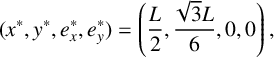 $$ \begin{align*} (x^{*},y^{*},e_{x}^{*},e_{y}^{*} )=\left(\frac{L}{2},\frac{\sqrt{3}L}{6},0,0\right),\end{align*} $$
with $e_{z}^{*}=\pm 1$
(as a consequence of
$e_{z}^{*}=\pm 1$
(as a consequence of $e_{x}^{*}=e_{y}^{*}=0$
). Note that
$e_{x}^{*}=e_{y}^{*}=0$
). Note that $(x^{*},y^{*})$
coincides with the centroid of the triangular cross-section and is invariant under the application of any operation from the associated symmetry group. The Jacobian matrix of (2.7) at the equilibrium pair is
$(x^{*},y^{*})$
coincides with the centroid of the triangular cross-section and is invariant under the application of any operation from the associated symmetry group. The Jacobian matrix of (2.7) at the equilibrium pair is
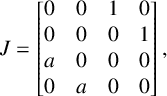 $$ \begin{align*} J= \begin{bmatrix} 0&0&1&0\\ 0&0&0&1\\ a&0&0&0\\ 0 &a & 0 & 0 \\ \end{bmatrix}, \end{align*} $$
where
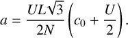 $$ \begin{align*}a=\frac{UL\sqrt{3}}{2N}\left(c_{0}+\frac{U}{2}\right).\end{align*} $$
Then, when $e_{z}^{*}=+1$
, we have
$e_{z}^{*}=+1$
, we have $c_{0}=1-U/2$
so that
$c_{0}=1-U/2$
so that $a=UL\sqrt {3}/2N>0$
. Similarly, when
$a=UL\sqrt {3}/2N>0$
. Similarly, when $e_{z}^{*}=-1$
, we have
$e_{z}^{*}=-1$
, we have $c_{0}=-1-U/2$
so that
$c_{0}=-1-U/2$
so that $a=-UL\sqrt {3}/2N<0$
.
$a=-UL\sqrt {3}/2N<0$
.
The characteristic polynomial equation of the matrix J is
 $$ \begin{align*} \lambda^{4}-2a\lambda^{2}+a^{2}=(\lambda^{2}-a)^{2}. \end{align*} $$
Thus, the roots of this quartic polynomial produce the eigenvalues of J,
 $$ \begin{align*}\lambda=\pm \sqrt{a}.\end{align*} $$
Therefore, the equilibrium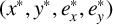 $(x^{*},y^{*},e_{x}^{*},e_{y}^{*})$
with
$(x^{*},y^{*},e_{x}^{*},e_{y}^{*})$
with $e_{z}^{*}=+1$
(and thus
$e_{z}^{*}=+1$
(and thus $a>0$
) is a saddle and thus unstable. However, with
$a>0$
) is a saddle and thus unstable. However, with $e_{z}^{*}=-1$
(and thus
$e_{z}^{*}=-1$
(and thus $a<0$
), the equilibrium is a centre.
$a<0$
), the equilibrium is a centre.
3.1 Behaviour of system near equilibrium points
To understand the active particle behaviour near equilibria, we calculate the eigenspace corresponding to the eigenvalues $\lambda =\pm \sqrt {a}$
. The eigenspace corresponding to
$\lambda =\pm \sqrt {a}$
. The eigenspace corresponding to $\lambda _{1}=- \sqrt {a}$
is
$\lambda _{1}=- \sqrt {a}$
is
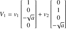 $$ \begin{align*}V_{1}=v_{1} \begin{bmatrix} 1\\ 0\\ - \sqrt{a}\\ 0 \end{bmatrix} +v_{2} \begin{bmatrix} 0\\ 1\\ 0\\ - \sqrt{a} \end{bmatrix}\end{align*} $$
and the eigenspace corresponding to $\lambda _{2}=\sqrt {a}$
is
$\lambda _{2}=\sqrt {a}$
is
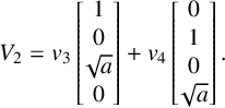 $$ \begin{align*}V_{2}=v_{3} \begin{bmatrix} 1\\ 0\\ \sqrt{a}\\ 0 \end{bmatrix}+v_{4} \begin{bmatrix} 0\\ 1\\ 0 \\ \sqrt{a} \end{bmatrix}.\end{align*} $$
Considering the case $a>0$
, for which the equilibrium is a saddle, then
$a>0$
, for which the equilibrium is a saddle, then $V_{1}$
corresponds to the tangent plane of the stable manifold whereas
$V_{1}$
corresponds to the tangent plane of the stable manifold whereas $V_{2}$
corresponds to the tangent plane of the unstable manifold.
$V_{2}$
corresponds to the tangent plane of the unstable manifold.
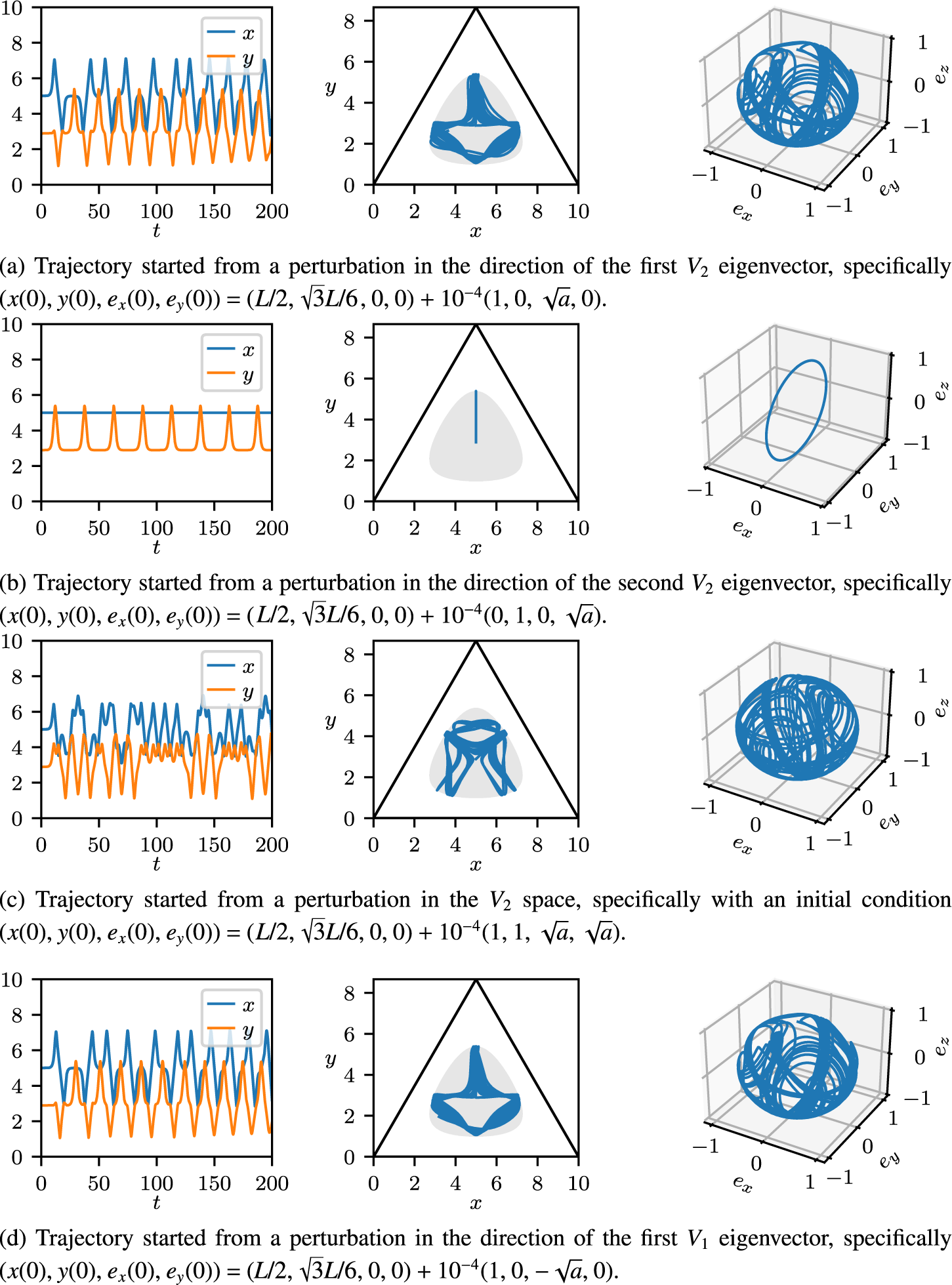
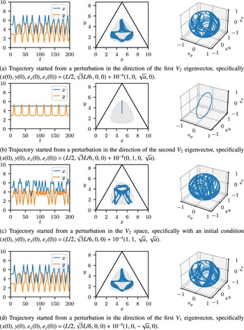
To understand the nature of trajectories on the stable and unstable manifold of the saddle equilibrium, we examine trajectories in which the initial condition is a small perturbation from the equilibrium point within the appropriate tangent plane. Figure 2 illustrates several examples of orbits initialized in this way with $L=U=10$
, in which case,
$L=U=10$
, in which case, $a=3/10$
. We observe that the behaviour of orbits occurring within a neighbourhood of the stable and unstable manifolds are quite distinctive, as was also the case in a square duct geometry [Reference Valani, Harding and Stokes20]. Figure 2(a) shows the result of a perturbation in the tangent plane of the unstable manifold with a positive x component. Over a short time period, the orbit resembles a somewhat exotic quasi-periodic orbit. Figure 2(b) shows the result of a perturbation in the tangent plane of the unstable manifold with a positive y component. This perturbation lies on the vertical axis of symmetry and, as a consequence, the orbit remains on that axis, that is, producing a periodic oscillation. Figure 2(c) shows the result of a similar perturbation aligned with one of the other axes of symmetry, that is, where the numerical rounding error means that the orbit cannot remain exactly on this axis of symmetry. Trajectories that are initialized via a perturbation using other combinations of the two eigenvectors associated with
$a=3/10$
. We observe that the behaviour of orbits occurring within a neighbourhood of the stable and unstable manifolds are quite distinctive, as was also the case in a square duct geometry [Reference Valani, Harding and Stokes20]. Figure 2(a) shows the result of a perturbation in the tangent plane of the unstable manifold with a positive x component. Over a short time period, the orbit resembles a somewhat exotic quasi-periodic orbit. Figure 2(b) shows the result of a perturbation in the tangent plane of the unstable manifold with a positive y component. This perturbation lies on the vertical axis of symmetry and, as a consequence, the orbit remains on that axis, that is, producing a periodic oscillation. Figure 2(c) shows the result of a similar perturbation aligned with one of the other axes of symmetry, that is, where the numerical rounding error means that the orbit cannot remain exactly on this axis of symmetry. Trajectories that are initialized via a perturbation using other combinations of the two eigenvectors associated with $V_2$
generally resemble a rotation of Figure 2(a). When trajectories are initialized via a perturbation in the tangent plane of the stable manifold, they are ultimately repelled from the saddle point and end up in a neighbourhood of the unstable manifold, as illustrated in Figure 2(d). We may instead integrate backwards in time, in which case, the stable manifold becomes the unstable manifold (and attracts orbits). Doing so produces orbits qualitatively similar to those already shown, which is to be expected as reversing time is equivalent to reversing the direction of flow and would not be expected to alter the qualitative nature of dynamics within the cross-section.
$V_2$
generally resemble a rotation of Figure 2(a). When trajectories are initialized via a perturbation in the tangent plane of the stable manifold, they are ultimately repelled from the saddle point and end up in a neighbourhood of the unstable manifold, as illustrated in Figure 2(d). We may instead integrate backwards in time, in which case, the stable manifold becomes the unstable manifold (and attracts orbits). Doing so produces orbits qualitatively similar to those already shown, which is to be expected as reversing time is equivalent to reversing the direction of flow and would not be expected to alter the qualitative nature of dynamics within the cross-section.
Active particle trajectories initialized from a small perturbation from the saddle equilibrium. In each example, we show the trace of $x(t)$
and
$x(t)$
and $y(t)$
(left), the trajectory within the triangular cross-section (middle) and the evolution of the orientation vector
$y(t)$
(left), the trajectory within the triangular cross-section (middle) and the evolution of the orientation vector $\mathbf {e}(t)$
(right). The parameters
$\mathbf {e}(t)$
(right). The parameters $U=10$
and
$U=10$
and $L=10$
were used, and
$L=10$
were used, and $e_z(0)=\sqrt {1-e_x(0)^{2}-e_y(0)^{2}}$
. A grey shaded region in the cross-section illustrates the basin as determined from the potential V occurring in the Hamiltonian.
$e_z(0)=\sqrt {1-e_x(0)^{2}-e_y(0)^{2}}$
. A grey shaded region in the cross-section illustrates the basin as determined from the potential V occurring in the Hamiltonian.
4 Describing the variety of active particle trajectories
To help describe and analyse the variety of possible active particle trajectories, a classification scheme was proposed by Valani et al. [Reference Valani, Harding and Stokes20] in the context of a square duct geometry. This classification scheme included notions of central swinging, vertical/horizontal swinging, wandering, tumbling and off-centre trapping motions, determined primarily by examining the region to which an orbit is confined. Subsequently, Harding et al. [Reference Harding, Valani and Stokes9] proposed a robust criteria for “tumbling” motion, in which a microswimmer continues to turn away from the centre of the cross-section before reaching it, based on examining the potential V associated with the Hamiltonian. A criteria to distinguish between “simple” and “complex” types of swinging/wandering motions was also proposed, with the “simple” case distinguished by having $e_z(t)<0$
for all t and “complex” being everything else which is not “tumbling”. To summarize the specific criteria, they proposed the following:
$e_z(t)<0$
for all t and “complex” being everything else which is not “tumbling”. To summarize the specific criteria, they proposed the following:
-
• tumbling occurs when $c_0>1-U/2$
(for which the basin is not simply connected);
$c_0>1-U/2$
(for which the basin is not simply connected); -
• complex swinging/wandering occurs when
$-U/2\leq c_0\leq 1-U/2$
(for which the basin is simply connected with the potential well attaining a local maxima at the centroid when
$c_0>-U/2$
, and the possible orientations exclude a spherical cap about
$\mathbf {e}=+\mathbf {k}$
when
$c_0<1-U/2$
); and -
• simple swinging/wandering occurs when
$c_0<-U/2$
(for which the basin is simply connected with the potential well attaining a local minimum at the centroid, the possible orientations are contained in a spherical cap about
$\mathbf {e}=-\mathbf {k}$
).







For the remainder of this section, we adapt the classification scheme from Valani et al. [Reference Valani, Harding and Stokes20] for the equilateral triangular duct geometry. This involves redefining the geometric confinement criteria, such as the central region and symmetry axes, with respect to the triangular symmetry while broadly maintaining the same hierarchy of classifications based on the regions within the cross-section that are visited by an orbit. This scheme provides more detail, especially for orbits confined to a neighbourhood of an axis of symmetry. Consequently, note that what we classify as “tumbling” herein will be a subset of those orbits for which $c_0>1-U/2$
(as defined tumbling in [Reference Harding, Valani and Stokes9]).
$c_0>1-U/2$
(as defined tumbling in [Reference Harding, Valani and Stokes9]).
4.1 Classification of active particle trajectories
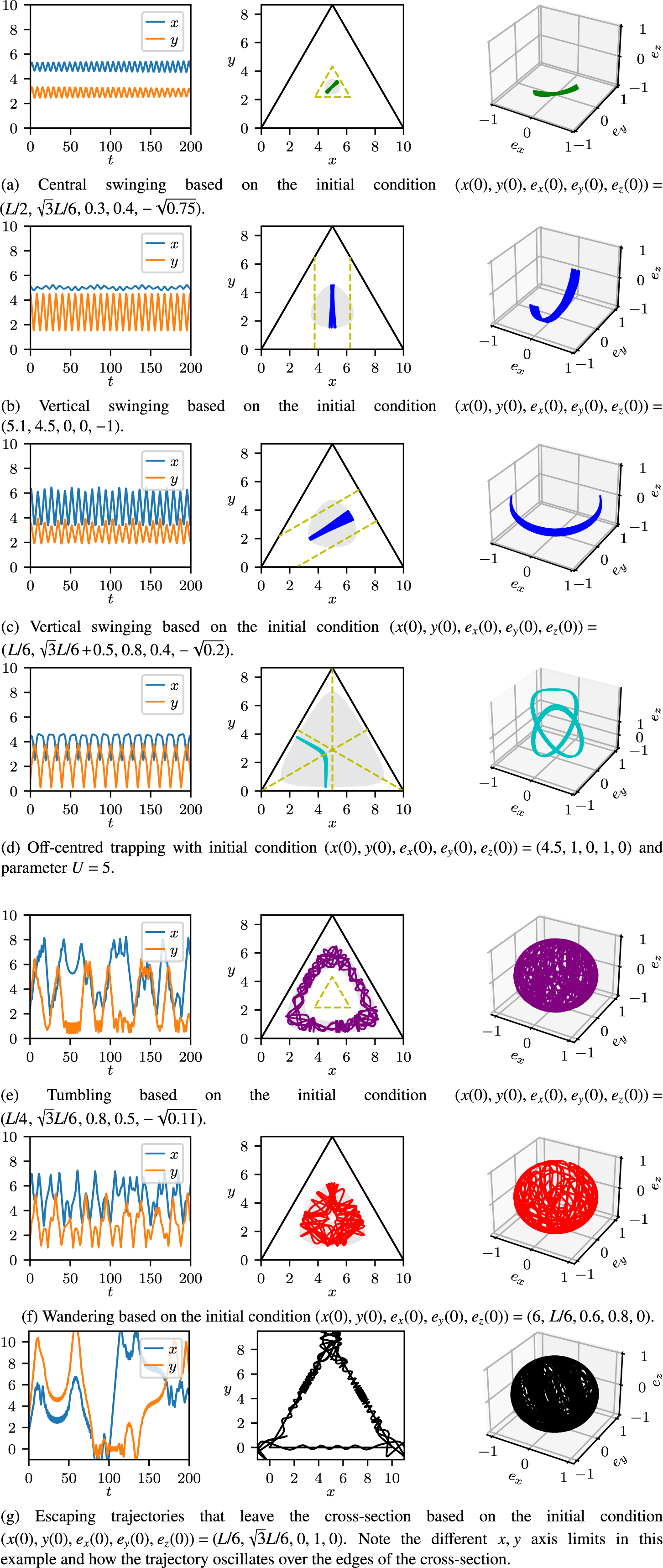
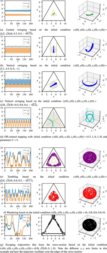
A variety of trajectories of active particles is observed by changing the relative fluid velocity scale U, and the initial position and orientation of the particle. We classify trajectories as one of six different types based on the regions they visit within the equilateral triangular cross-section. Each type has been assigned a colour to facilitate presentation of the results. The distinct types are described as follows, listed in order of precedence with respect to the procedure by which trajectories are classified.
-
(i) Escaping motion (black)—trajectories that exit the cross-section. There is no mechanism in the model (described by (2.7)) that prevents a particle passing through the duct walls, especially as the given
$\bar {w}(x,y)$
is well-defined on all of
$\mathbb {R}^2$
. -
(ii) Central swinging motion (green)—trajectories that exhibit swinging motion in their orientation as they oscillate within a small neighbourhood of the centroid, specifically remaining within a similar triangle with side length
$L/4$
. -
(iii) Vertical swinging motion (blue)—trajectories that exhibit swinging motion in their orientation as they oscillate by a significant amount in the vertical y direction while remaining confined in the x direction, specifically within
$L/8$
of the vertical axis of symmetry. Furthermore, trajectories that are similarly confined near the other axes of symmetry are also classified as “vertical” swinging. -
(iv) Off-centred trapping (cyan)—trajectories that exhibit confinement away from the centroid and do not intersect at least one axis of symmetry.
-
(v) Tumbling motion (purple)—trajectories that are confined away from a relatively large neighbourhood of the centroid and surround it, specifically avoiding a similar triangle with side length
$L/4$
and intersecting every axis of symmetry. -
(vi) Wandering motion (red)—trajectories that do not satisfy any of the above criteria. These are generally confined to a region near/containing the centroid, are neither central nor vertical swinging and visit close enough to the centroid so as not to be tumbling.


Observe that each of these criteria can be readily assessed by monitoring $x(t),y(t)$
throughout a calculation/simulation. With the parameters
$x(t),y(t)$
throughout a calculation/simulation. With the parameters $L=U=10$
used for most examples herein, a simulation time of
$L=U=10$
used for most examples herein, a simulation time of $O(100)$
is generally enough to correctly classify an orbit.
$O(100)$
is generally enough to correctly classify an orbit.
Examples of each of the six classifications are illustrated in Figure 3 (with two examples of “vertical” swinging), noting that in each example, the path of the trajectory within physical and orientation space has been coloured according to the assigned classification. We later use the colours assigned to each classification to examine the nature of orbits under a wide range of initial conditions and parameter values in Section 5.
Different examples of active particle motion. Each row shows the $x,y$
coordinates as a function of t (left), the
$x,y$
coordinates as a function of t (left), the $(x,y)$
trajectory within the cross-section (middle) and the trajectory of
$(x,y)$
trajectory within the cross-section (middle) and the trajectory of $\mathbf {e}$
on the surface of the unit sphere (right). The colour of trajectories in the right two plots represent the classification: green—central swinging motion; blue—vertical swinging motion; purple—tumbling motion; cyan—off-centred trapping motion; red—wandering motion; and black—for trajectories that leave the cross-section. Remaining parameters were fixed as
$\mathbf {e}$
on the surface of the unit sphere (right). The colour of trajectories in the right two plots represent the classification: green—central swinging motion; blue—vertical swinging motion; purple—tumbling motion; cyan—off-centred trapping motion; red—wandering motion; and black—for trajectories that leave the cross-section. Remaining parameters were fixed as $U=10$
and
$U=10$
and $L=10$
in each panel with the exception of Figure 3(d), where
$L=10$
in each panel with the exception of Figure 3(d), where $U=5$
. In each case, exempting the escaping trajectory, a grey shaded region in the cross-section illustrates the basin as determined from the potential V occurring in the Hamiltonian.
$U=5$
. In each case, exempting the escaping trajectory, a grey shaded region in the cross-section illustrates the basin as determined from the potential V occurring in the Hamiltonian.
4.2 Examples of exotic trajectories
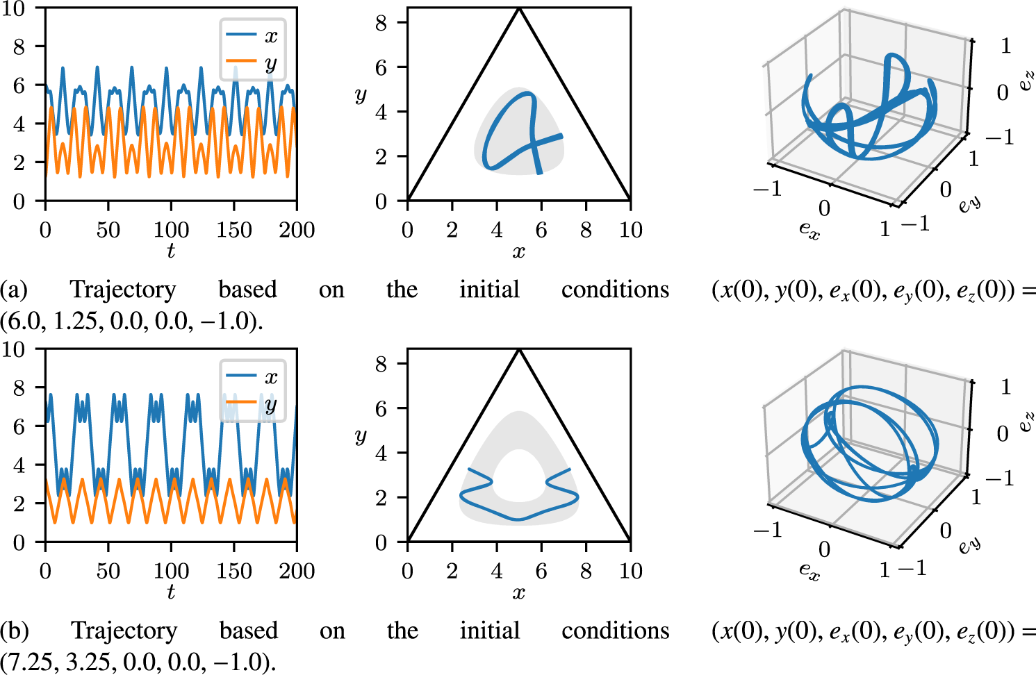
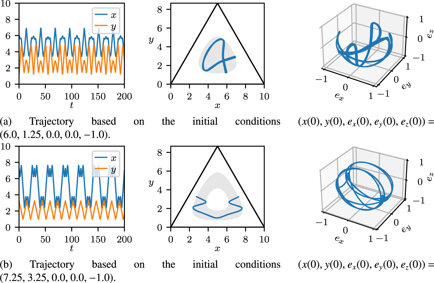
While the above classification scheme gives a reasonably good overview of the types of trajectories that are typically observed, it is sometimes possible to find trajectories with distinctive characteristics compared with others of a given type. Two such examples are shown in Figure 4. Figure 4(a) illustrates a quasi-periodic trajectory (almost periodic, one might argue) consisting of a loop around the centroid which crosses itself before returning along a very similar path. While this would be classified as wandering in the classification scheme described above, it is clearly distinct when compared with more typical examples of wandering trajectories (that is, which are similar to Figure 3f). Figure 4(b) illustrates a periodic trajectory consisting of an intricate multi-wave oscillation which does not enclose the centroid. Under our classification of this scheme, this orbit would be considered tumbling, but it is clearly distinct from other tumbling trajectories (which are generally similar to Figure 3e). One might refer to such trajectories as “exotic”. Apart from being (quasi-)periodic, they are generally not straightforward to identify (programmatically) and uniquely classify.
Additional examples of active particle trajectories. The x and y trajectories of the active particles, as well as the trajectories of active particles in an equilateral triangular channel are illustrated in the $(x,y)$
plane and to the right, the 3D plots illustrate the orientations of the particles. A grey shaded region in the cross-section illustrates the basin as determined from the potential V occurring in the Hamiltonian. We use
$(x,y)$
plane and to the right, the 3D plots illustrate the orientations of the particles. A grey shaded region in the cross-section illustrates the basin as determined from the potential V occurring in the Hamiltonian. We use $L=10$
and
$L=10$
and $U=10$
in each example.
$U=10$
in each example.
5 Analysing the distribution of active particle motion
We investigate the broad distribution of the various types of active particle motion that occur within an equilateral triangular channel. We use the classification scheme and associated colour scheme of Section 4.1 to illustrate which types of motion occur under a range of different initial conditions and values of the parameter U. We note that exotic trajectories, such as those identified in Section 4.2, have not been separately classified within the results of this section (with such examples generally classified as wandering or tumbling, depending on how close they come to the centroid).
5.1 Effects of initial conditions
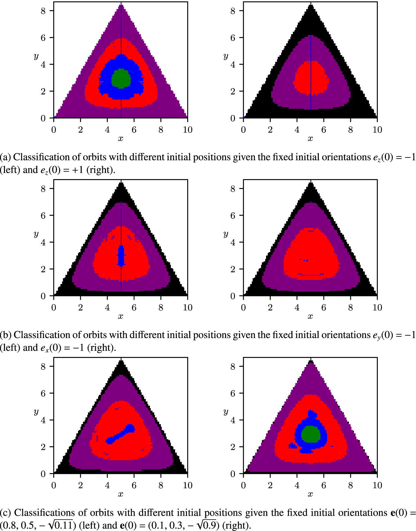
Recall that the dynamics of the active particle is governed by a four-dimensional nonlinear dynamical system (2.7), which requires the five initial conditions $\mathbf {e}(0)$
,
$\mathbf {e}(0)$
, $x(0)$
,
$x(0)$
, $y(0)$
, noting
$y(0)$
, noting $e_z(0)$
effectively determines the constant
$e_z(0)$
effectively determines the constant $c_0$
. Initially, we consider a fixed initial orientation and vary
$c_0$
. Initially, we consider a fixed initial orientation and vary $(x(0), y(0))$
within the cross-section with fixed
$(x(0), y(0))$
within the cross-section with fixed $U=10$
. Figure 5 illustrates the resulting classifications as a function of
$U=10$
. Figure 5 illustrates the resulting classifications as a function of $(x(0), y(0))$
for six different initial orientations.
$(x(0), y(0))$
for six different initial orientations.
Trajectory classification with varying initial position ( $x(0),y(0)$
) for fixed
$x(0),y(0)$
) for fixed $U=10$
and several given fixed initial orientations. The colours indicate the classification of each trajectory: green—central swinging motion; blue—vertical swinging motion; purple—tumbling motion; red—wandering motion; and black—escaping trajectories.
$U=10$
and several given fixed initial orientations. The colours indicate the classification of each trajectory: green—central swinging motion; blue—vertical swinging motion; purple—tumbling motion; red—wandering motion; and black—escaping trajectories.
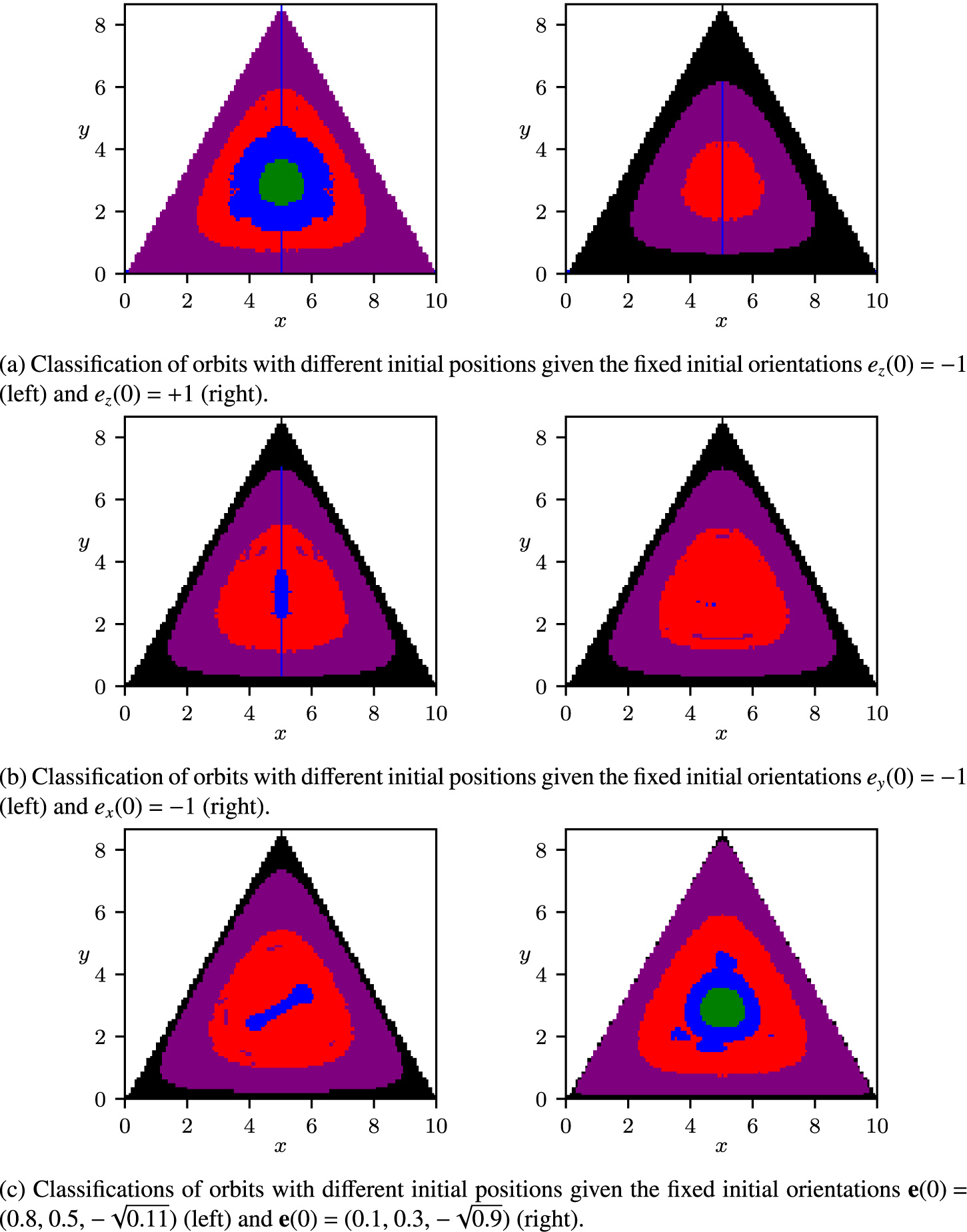
Figure 5(a) shows the variety of active particle trajectories that occur given the upstream and downstream oriented initial conditions $e_z(0)=\pm 1$
. For
$e_z(0)=\pm 1$
. For $e_z(0)=-1$
(left), the graph shows an inner region of central swinging motion in which active particles generally exhibit a relatively simple oscillation about the centroid. This is surrounded by a blue region, indicating “vertical” swinging motion in which particles oscillate close to an axis of symmetry. This includes a distinct region aligned with the vertical axis of symmetry. Such a segment is expected, but not observed, along the other axes of symmetry. The primary reason for their absence is the irrational slope of the other two axes of symmetry, which leads to rounding errors that grow over time and ultimately prevents orbits from remaining on these axes. The red region indicates wandering motion, remaining somewhat centrally confined, but generally starting to be more complex than central and vertical swinging motions. The outer purple region represents tumbling motion and generally consists of chaotic behaviour away from the centre (as illustrated later). Conversely, with
$e_z(0)=-1$
(left), the graph shows an inner region of central swinging motion in which active particles generally exhibit a relatively simple oscillation about the centroid. This is surrounded by a blue region, indicating “vertical” swinging motion in which particles oscillate close to an axis of symmetry. This includes a distinct region aligned with the vertical axis of symmetry. Such a segment is expected, but not observed, along the other axes of symmetry. The primary reason for their absence is the irrational slope of the other two axes of symmetry, which leads to rounding errors that grow over time and ultimately prevents orbits from remaining on these axes. The red region indicates wandering motion, remaining somewhat centrally confined, but generally starting to be more complex than central and vertical swinging motions. The outer purple region represents tumbling motion and generally consists of chaotic behaviour away from the centre (as illustrated later). Conversely, with $e_z(0)=1$
(right), central swinging motion vanishes, vertical swinging occurs only on the vertical axis of symmetry (and is once more absent from other axes of symmetry due to rounding errors), the regions of wandering and tumbling motion shrink, and a black region of escaping trajectories appears in a neighbourhood of the cross-section boundaries. The existence of the escaping region can be explained by orbits no longer being confined to the duct cross-section and is evident by an examination of the potential [Reference Harding, Valani and Stokes9] (noting again that this model has no mechanism to account for particle–wall collisions and that the cubic description of
$e_z(0)=1$
(right), central swinging motion vanishes, vertical swinging occurs only on the vertical axis of symmetry (and is once more absent from other axes of symmetry due to rounding errors), the regions of wandering and tumbling motion shrink, and a black region of escaping trajectories appears in a neighbourhood of the cross-section boundaries. The existence of the escaping region can be explained by orbits no longer being confined to the duct cross-section and is evident by an examination of the potential [Reference Harding, Valani and Stokes9] (noting again that this model has no mechanism to account for particle–wall collisions and that the cubic description of $\bar {w}(x,y)$
in this example is well-defined beyond the cross-section, albeit being non-physical in the fluid flow context).
$\bar {w}(x,y)$
in this example is well-defined beyond the cross-section, albeit being non-physical in the fluid flow context).
Figure 5(b) shows the variety in classifications given initial orientations of ${e_y(0)=-1}$
(left) and
${e_y(0)=-1}$
(left) and $e_x(0)=-1$
(right). In both cases, there is an absence of central swinging motion and an identical black region of escaping trajectories. The case
$e_x(0)=-1$
(right). In both cases, there is an absence of central swinging motion and an identical black region of escaping trajectories. The case $e_y=-1$
possesses a region of vertical swinging motion, given the alignment of this initial orientation with the vertical axis of symmetry, but there is no such region in the case of
$e_y=-1$
possesses a region of vertical swinging motion, given the alignment of this initial orientation with the vertical axis of symmetry, but there is no such region in the case of $e_x(0)=-1$
. Note that we should not expect to observe
$e_x(0)=-1$
. Note that we should not expect to observe $120^\circ $
symmetry with these choices of initial orientation. The wandering motion shown by the red region and tumbling motion represented by purple regions are otherwise broadly consistent between the two plots. Although not shown here, the graphs obtained with initial orientations of
$120^\circ $
symmetry with these choices of initial orientation. The wandering motion shown by the red region and tumbling motion represented by purple regions are otherwise broadly consistent between the two plots. Although not shown here, the graphs obtained with initial orientations of $e_y(0)=+1$
and
$e_y(0)=+1$
and $e_x(0)=+1$
are very similar to those shown with the opposite initial orientation. Specifically, the
$e_x(0)=+1$
are very similar to those shown with the opposite initial orientation. Specifically, the $e_x(0)=+1$
case is a horizontal reflection of the
$e_x(0)=+1$
case is a horizontal reflection of the $e_x(0)=-1$
case, as one would expect, while the
$e_x(0)=-1$
case, as one would expect, while the $e_y(0)=+1$
case is qualitatively similar to the
$e_y(0)=+1$
case is qualitatively similar to the $e_y(0)=-1$
case, but with some minor differences near the boundary between each region.
$e_y(0)=-1$
case, but with some minor differences near the boundary between each region.
Figure 5(c) shows the result with initial orientations $\mathbf {e}(0)=(0.8,0.5,-\sqrt {0.11})$
(left) and
$\mathbf {e}(0)=(0.8,0.5,-\sqrt {0.11})$
(left) and $\mathbf {e}(0)=(0.1,0.3,-\sqrt {0.9})$
(right). These initial orientations were chosen so as not to align with any coordinate nor symmetry axis, whilst still having unit magnitude. The general pattern of a central swinging region (if it exists), surrounded by vertical swinging, then wandering, then tumbling and finally an escaping region (if it exists), persists. Of course, with these non-axis-aligned initial orientations, the specific details are slightly more complex and lack symmetry.
$\mathbf {e}(0)=(0.1,0.3,-\sqrt {0.9})$
(right). These initial orientations were chosen so as not to align with any coordinate nor symmetry axis, whilst still having unit magnitude. The general pattern of a central swinging region (if it exists), surrounded by vertical swinging, then wandering, then tumbling and finally an escaping region (if it exists), persists. Of course, with these non-axis-aligned initial orientations, the specific details are slightly more complex and lack symmetry.
To examine the prominence of different classifications, with the fixed parameters $U=L=10$
, we classified 277 000 orbits over the four-dimensional initial condition space (specifically using 1108 points in the cross-section and 250 distributed over the sphere). These results show that approximately 27.6% of orbits analysed are escaping, being concentrated around the edges of the cross-section with
$U=L=10$
, we classified 277 000 orbits over the four-dimensional initial condition space (specifically using 1108 points in the cross-section and 250 distributed over the sphere). These results show that approximately 27.6% of orbits analysed are escaping, being concentrated around the edges of the cross-section with $e_z(0)>-1$
, after which 44.4% are tumbling, 25.0% are wandering, 2.7% are vertical swinging, 0.3% are central swinging and only a single orbit was identified as exhibiting off-centre trapping. This suggests that instances of central and vertical swinging may be somewhat over-represented in the examples of Figure 5, although the general order of prominence is consistent.
$e_z(0)>-1$
, after which 44.4% are tumbling, 25.0% are wandering, 2.7% are vertical swinging, 0.3% are central swinging and only a single orbit was identified as exhibiting off-centre trapping. This suggests that instances of central and vertical swinging may be somewhat over-represented in the examples of Figure 5, although the general order of prominence is consistent.
5.2 Effects of the relative fluid velocity scale
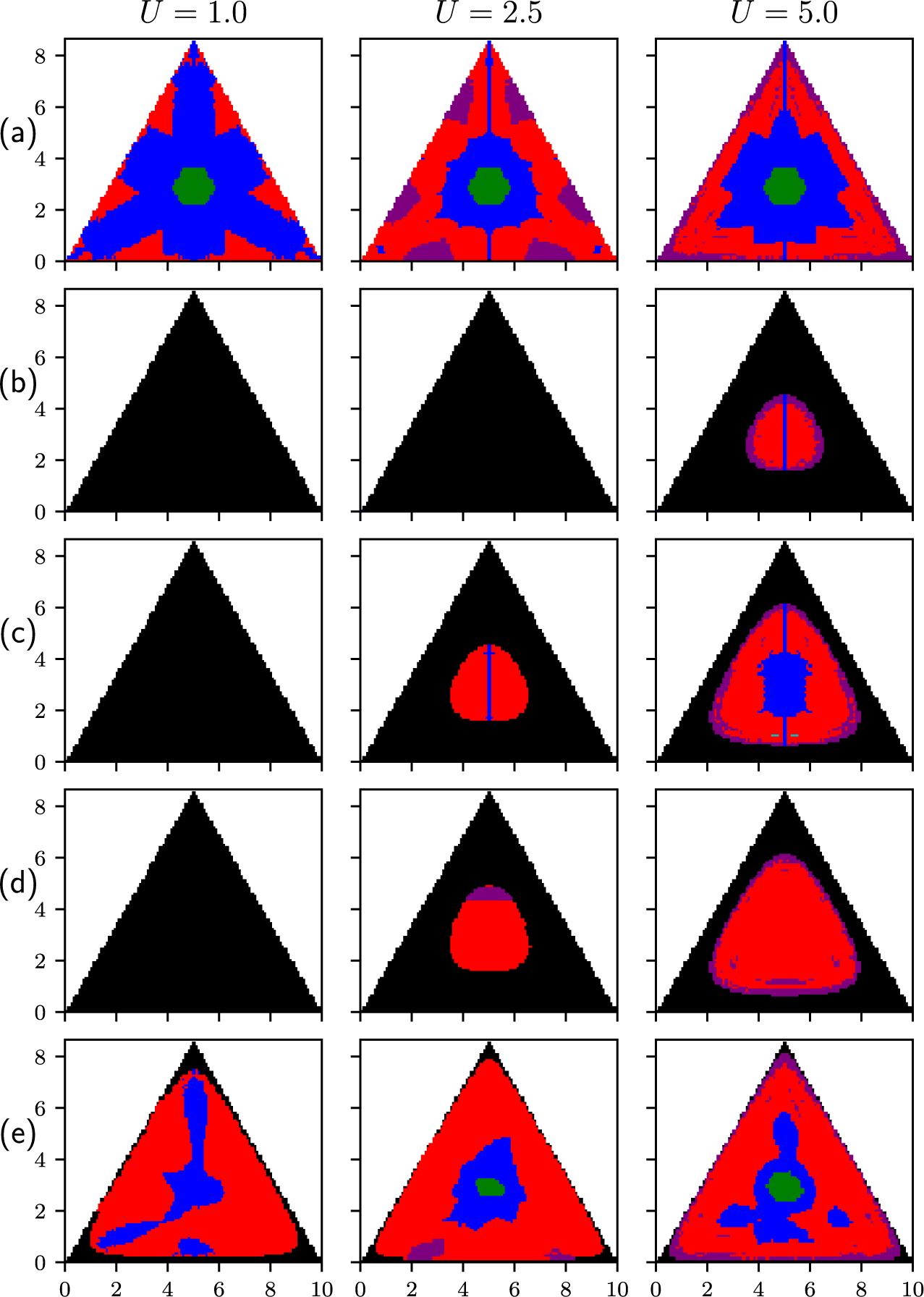
We now examine the variations in the dynamics of active particles with respect to the parameter U, denoting the maximum fluid velocity relative to the intrinsic particle swimming velocity. In particular, we examine the variation in particle trajectory classification with respect to $(x(0),y(0))$
for the different values
$(x(0),y(0))$
for the different values $U=1$
,
$U=1$
, $U=2.5$
and
$U=2.5$
and $U=5$
, and with several fixed initial orientations (as previously examined with
$U=5$
, and with several fixed initial orientations (as previously examined with $U=10$
in Figure 5). The results of this analysis are shown in Figure 6.
$U=10$
in Figure 5). The results of this analysis are shown in Figure 6.
Trajectory classification in the initial position plane ( $x(0),y(0)$
) for
$x(0),y(0)$
) for $U=1$
,
$U=1$
, $U=2.5$
and
$U=2.5$
and $U=5$
(left to right in each row), and the fixed initial orientations: (a)
$U=5$
(left to right in each row), and the fixed initial orientations: (a) $\mathbf {e}(0)=(0,0,-1)$
; (b)
$\mathbf {e}(0)=(0,0,-1)$
; (b) $\mathbf {e}(0)=(0,0,1)$
; (c)
$\mathbf {e}(0)=(0,0,1)$
; (c) $\mathbf {e}(0)=(0,-1,0)$
; (d)
$\mathbf {e}(0)=(0,-1,0)$
; (d) $\mathbf {e}(0)=(-1,0,0)$
; and (e)
$\mathbf {e}(0)=(-1,0,0)$
; and (e) $\mathbf {e}(0)=(0.1,0.3,-\sqrt {0.9})$
. The different colours represent the classification of trajectories: green—central swinging motion; blue—vertical swinging motion; purple—tumbling motion; cyan—off-centred trapping motion; red—wandering motion; and black—escaping trajectories.
$\mathbf {e}(0)=(0.1,0.3,-\sqrt {0.9})$
. The different colours represent the classification of trajectories: green—central swinging motion; blue—vertical swinging motion; purple—tumbling motion; cyan—off-centred trapping motion; red—wandering motion; and black—escaping trajectories.
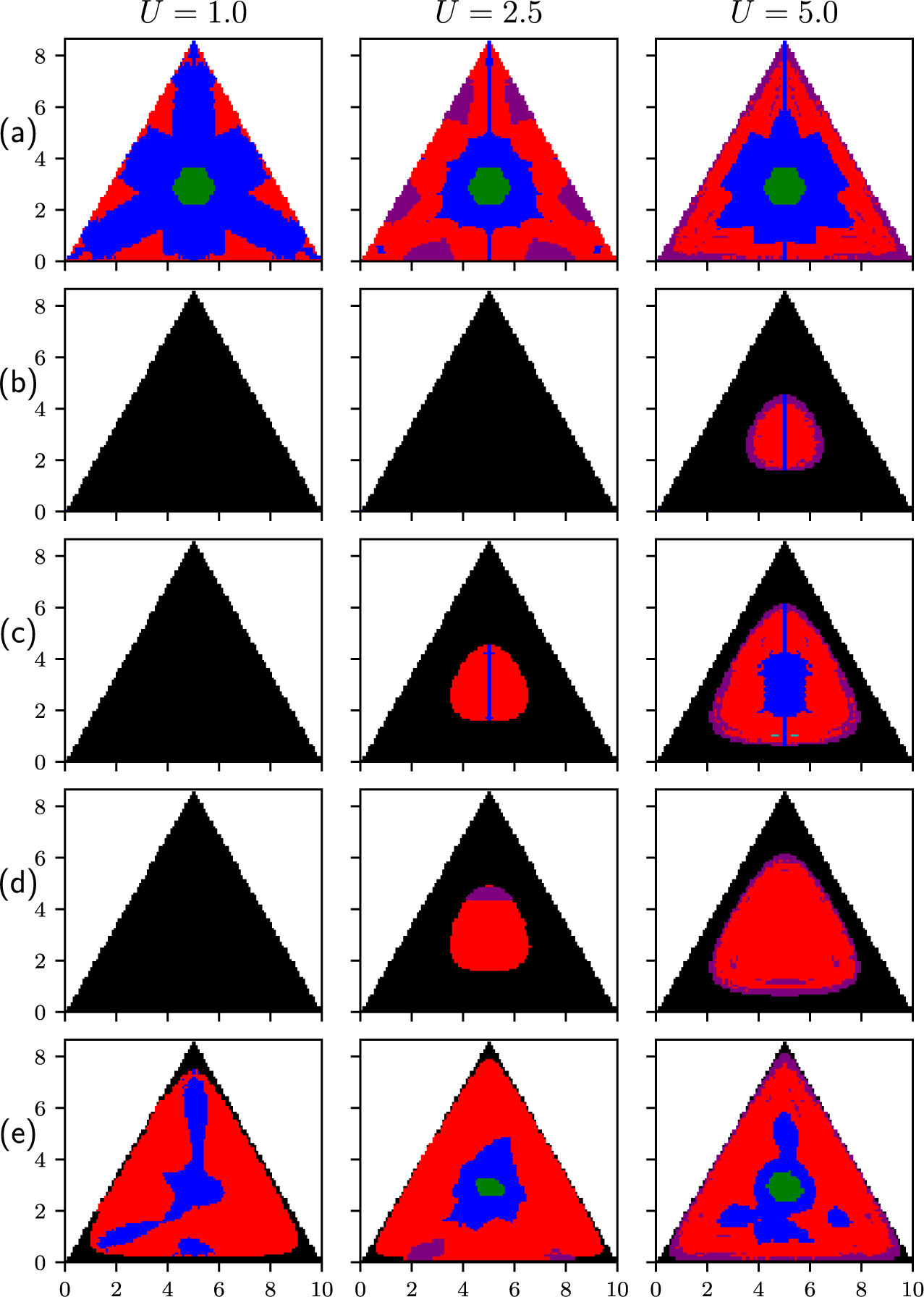
Figure 6(a) shows the effect of U given different initial positions and a fixed initial orientation of $e_z(0)=-1$
. In this particular case, orbits always remain confined within the cross-section. With
$e_z(0)=-1$
. In this particular case, orbits always remain confined within the cross-section. With $U=1$
(left), there is a significantly enlarged region of “vertical” swinging motion surrounding an inner region of central swinging motion. Some small regions of wandering motion are observed near the walls of the cross-section. With increasing U (left to right), the region of vertical swinging shrinks and is replaced by wandering motion, and some small regions of tumbling motion appear around the boundaries. Although we should expect three-fold symmetry in each of these examples, some deviations are evident, especially on the non-vertical axes of symmetry, due to rounding errors.
$U=1$
(left), there is a significantly enlarged region of “vertical” swinging motion surrounding an inner region of central swinging motion. Some small regions of wandering motion are observed near the walls of the cross-section. With increasing U (left to right), the region of vertical swinging shrinks and is replaced by wandering motion, and some small regions of tumbling motion appear around the boundaries. Although we should expect three-fold symmetry in each of these examples, some deviations are evident, especially on the non-vertical axes of symmetry, due to rounding errors.
Figure 6(b) shows the effect of U given different initial positions and a fixed initial orientation of $e_z(0)=+1$
. For
$e_z(0)=+1$
. For $U=1$
and
$U=1$
and $U=2.5$
, the trajectories are all escaping, while in the case
$U=2.5$
, the trajectories are all escaping, while in the case $U=5$
, there is a small region of non-escaping trajectories, mostly wandering surrounded by a thin region of tumbling and with a vertical strip of vertical swinging motion.
$U=5$
, there is a small region of non-escaping trajectories, mostly wandering surrounded by a thin region of tumbling and with a vertical strip of vertical swinging motion.
Figure 6(c) shows the case with fixed initial orientation of $e_y(0)=-1$
, noting a near identical result is obtained with
$e_y(0)=-1$
, noting a near identical result is obtained with $e_y(0)=+1$
. Escaping motion is again generally dominant, albeit to a lesser extent than the case of
$e_y(0)=+1$
. Escaping motion is again generally dominant, albeit to a lesser extent than the case of $e_z(0)=+1$
. A new feature observed when
$e_z(0)=+1$
. A new feature observed when $U=5$
is some very small regions of off-centred trapping motion. Figure 6(d) shows the analogous case with fixed initial orientation of
$U=5$
is some very small regions of off-centred trapping motion. Figure 6(d) shows the analogous case with fixed initial orientation of $e_x(0)=-1$
, noting a near identical result is obtained with
$e_x(0)=-1$
, noting a near identical result is obtained with $e_x(0)=+1$
. The regions of escaping motion are identical to those of the
$e_x(0)=+1$
. The regions of escaping motion are identical to those of the $e_y(0)=-1$
case, the main difference between the two being a lack of vertical swinging motion here (and no off-centred trapping).
$e_y(0)=-1$
case, the main difference between the two being a lack of vertical swinging motion here (and no off-centred trapping).
Figure 6(e) shows the results obtained with the initial orientation ${\mathbf {e}(0)=(0.1,0.3, -\sqrt {0.9})}$
. For each U, a large region of wandering motion is dominant, with variations in the regions of vertical swinging and central swinging with increasing U.
${\mathbf {e}(0)=(0.1,0.3, -\sqrt {0.9})}$
. For each U, a large region of wandering motion is dominant, with variations in the regions of vertical swinging and central swinging with increasing U.
Effectively, with smaller values of U, the orientation of the active particle is rotated too slowly, which provides greater opportunity for the particle to escape the cross-section when it is directed towards a wall. Simultaneously, it is more difficult for the active particle to tumble and thereby avoid the centre of the cross-section, thus significantly reducing the observed regions of tumbling motion.
6 Examination of chaotic behaviour
We now illustrate some indicators of chaotic motion through the use of Poincaré sections and Lyapunov exponents. Throughout this section, we use $L=10$
and
$L=10$
and $U=10$
.
$U=10$
.
6.1 Poincaré sections
Using Poincaré sections, we examine the nature of system dynamics and transition to chaos. We construct Poincaré maps for this system in the following way. First, we choose a value of $c_0$
, the most interesting choices being near
$c_0$
, the most interesting choices being near $-U/2$
. Next, we generate several initial conditions (
$-U/2$
. Next, we generate several initial conditions ( $(x(0),y(0))$
and
$(x(0),y(0))$
and $\mathbf {e}(0)$
) which produce the chosen
$\mathbf {e}(0)$
) which produce the chosen $c_0$
. For each of those initial conditions, we then solve (2.7) to produce a trajectory for which we then identify times
$c_0$
. For each of those initial conditions, we then solve (2.7) to produce a trajectory for which we then identify times $t_n\geq 0$
for which the
$t_n\geq 0$
for which the $e_y=0$
hyperplane is crossed in the positive direction. At each of these
$e_y=0$
hyperplane is crossed in the positive direction. At each of these $t_n$
, we record the values
$t_n$
, we record the values $e_x(t_n)$
,
$e_x(t_n)$
, $e_z(t_n)$
and
$e_z(t_n)$
and $x(t_n)$
. We define the angle
$x(t_n)$
. We define the angle $\theta _n$
such that
$\theta _n$
such that $e_x(t_n)=\sin (\theta _n)$
and
$e_x(t_n)=\sin (\theta _n)$
and $e_z(t_n)=\cos (\theta _n)$
. Subsequently, we plot
$e_z(t_n)=\cos (\theta _n)$
. Subsequently, we plot $\theta _n$
against
$\theta _n$
against $x(t_n)$
to produce a Poincaré section. The points are coloured according to their classification. Several examples are shown in Figure 7.
$x(t_n)$
to produce a Poincaré section. The points are coloured according to their classification. Several examples are shown in Figure 7.
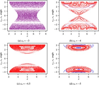
Poincaré sections for fixed parameter $U=10$
obtained using various initial conditions satisfying the chosen
$U=10$
obtained using various initial conditions satisfying the chosen $c_0$
, as given in each sub-caption, and examining each such trajectory when
$c_0$
, as given in each sub-caption, and examining each such trajectory when $e_y=0$
is crossed in the positive direction. The different colours represent different trajectories: blue—vertical swinging motion, purple—tumbling motion; and red—wandering motion. Note that escaping trajectories have been omitted.
$e_y=0$
is crossed in the positive direction. The different colours represent different trajectories: blue—vertical swinging motion, purple—tumbling motion; and red—wandering motion. Note that escaping trajectories have been omitted.
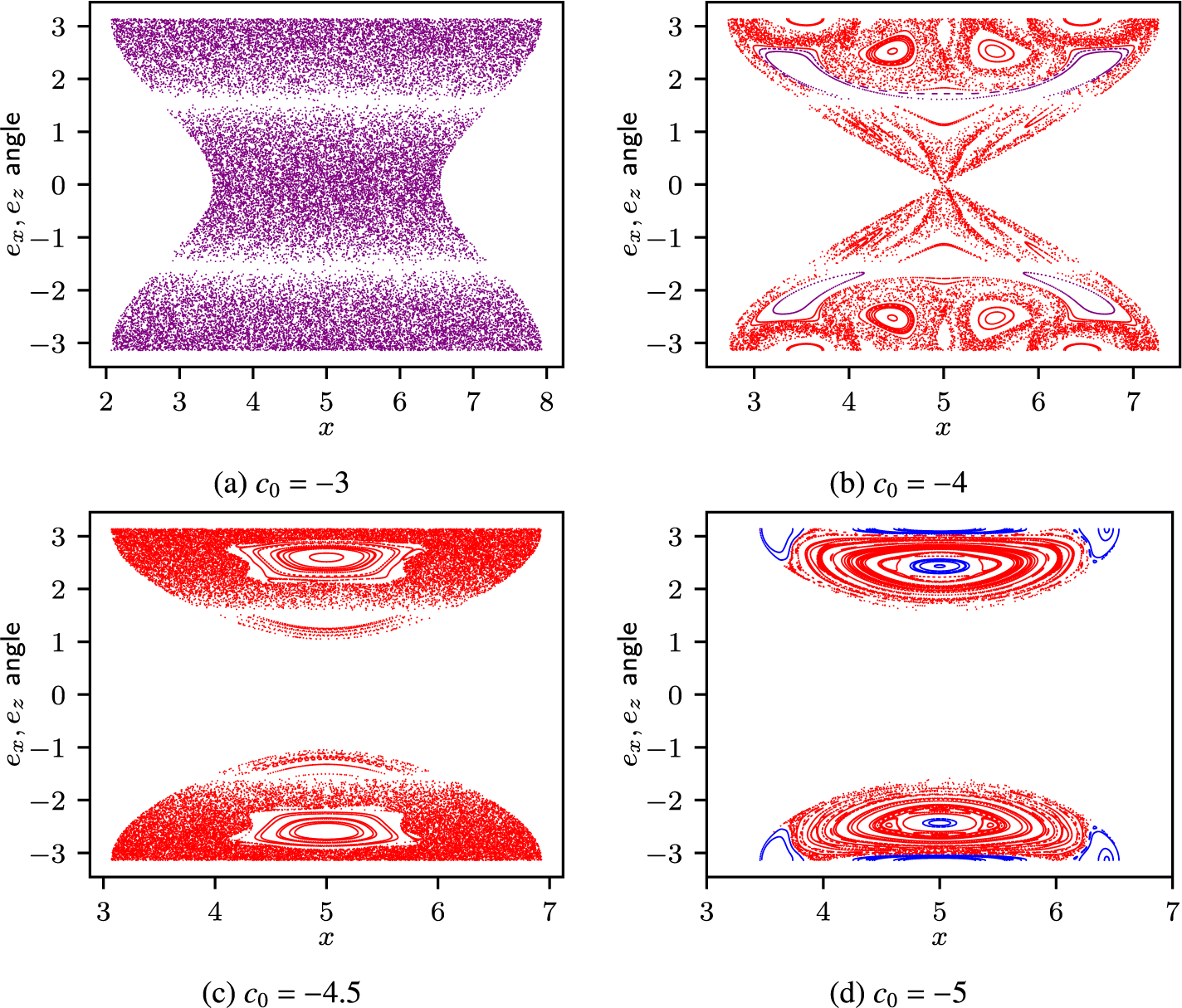
Figure 7a illustrates the case $c_0=-3$
. All of the trajectories produced for this value of
$c_0=-3$
. All of the trajectories produced for this value of $c_0$
are tumbling and the reasonably dense distribution of points is indicative of these orbits all being chaotic. Figure 7(b) illustrates the case
$c_0$
are tumbling and the reasonably dense distribution of points is indicative of these orbits all being chaotic. Figure 7(b) illustrates the case $c_0=-4$
. The majority of trajectories produced for this value of
$c_0=-4$
. The majority of trajectories produced for this value of $c_0$
are wandering, albeit with a relatively small number of tumbling as well. Here, we see points organized as closed curves, indicative of quasi-periodic motion, coexisting with regions of a somewhat dense scattering of points, indicative of chaotic motion. Figure 7(c) illustrates the case
$c_0$
are wandering, albeit with a relatively small number of tumbling as well. Here, we see points organized as closed curves, indicative of quasi-periodic motion, coexisting with regions of a somewhat dense scattering of points, indicative of chaotic motion. Figure 7(c) illustrates the case $c_0=-4.5$
, which consists entirely of wandering motion and again illustrates the coexistence of both quasi-periodic and chaotic motion. Figure 7(d) illustrates the case
$c_0=-4.5$
, which consists entirely of wandering motion and again illustrates the coexistence of both quasi-periodic and chaotic motion. Figure 7(d) illustrates the case $c_0=-5$
, which consists of wandering and vertical swinging motion and primarily indicates quasi-periodic motion.
$c_0=-5$
, which consists of wandering and vertical swinging motion and primarily indicates quasi-periodic motion.
We draw several conclusions from this. The first is that there appears to be a decreasing prevalence of quasi-periodic motion with increasing $c_0$
. The second is that swinging motion occurs for smaller
$c_0$
. The second is that swinging motion occurs for smaller $c_0$
and tumbling for larger
$c_0$
and tumbling for larger $c_0$
, with wandering in between. Both of these can be explained by larger values of
$c_0$
, with wandering in between. Both of these can be explained by larger values of $c_0$
generally corresponding to orbits possessing more energy, that is, by considering the magnitude of the potential V evaluated at the centre of the cross-section. In addition, we note that the diminishing domain in which points occur in Figure 7 with decreasing
$c_0$
generally corresponding to orbits possessing more energy, that is, by considering the magnitude of the potential V evaluated at the centre of the cross-section. In addition, we note that the diminishing domain in which points occur in Figure 7 with decreasing $c_0$
is due to the way in which the potential restricts the allowable combinations of
$c_0$
is due to the way in which the potential restricts the allowable combinations of $x,y,e_z$
[Reference Harding, Valani and Stokes9]. Moreover, we have not included an example with larger values of
$x,y,e_z$
[Reference Harding, Valani and Stokes9]. Moreover, we have not included an example with larger values of $c_0$
in which escaping orbits begin to occur.
$c_0$
in which escaping orbits begin to occur.
6.2 Largest Lyapunov exponent
The presence of chaos in the trajectories can be quantified by computing the largest Lyapunov exponent (LLE) of the underlying nonlinear dynamical system. A zero LLE indicates that the motion of an active particle is either periodic or quasi-periodic, whereas a positive LLE indicates that the motion is chaotic (with the degree of sensitivity to initial conditions indicated by the magnitude of LLE). Herein, we estimate the LLE by explicitly solving the variational problem associated with (2.7) (see [Reference Harding, Valani and Stokes9]). Specifically, letting $A(t)$
denote the Jacobian of (2.7), we solve the initial value problem
$A(t)$
denote the Jacobian of (2.7), we solve the initial value problem
 $$ \begin{align*} M'(t) = A(t)\cdot M(t) , \quad M(0)=I_4 , \end{align*} $$
simultaneously with (2.7), where $I_4$
denotes the
$I_4$
denotes the $4\times 4$
identity matrix. The asymptotic growth of the singular values of M subsequently informs the Lyapunov numbers. Gram–Schmidt orthogonalization is applied periodically to
$4\times 4$
identity matrix. The asymptotic growth of the singular values of M subsequently informs the Lyapunov numbers. Gram–Schmidt orthogonalization is applied periodically to $M(t)$
to stabilize this calculation.
$M(t)$
to stabilize this calculation.
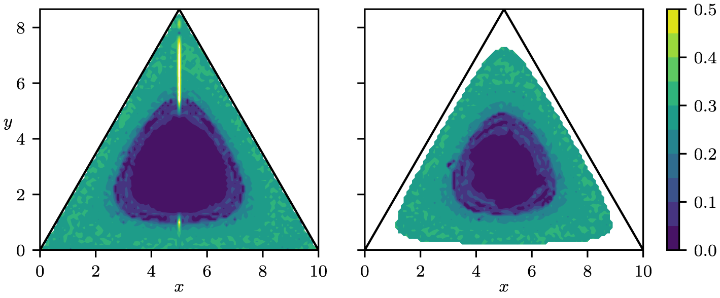
Figure 8 shows an example of the LLE plotted with respect to the initial position $(x(0),y(0))$
given the fixed initial orientations
$(x(0),y(0))$
given the fixed initial orientations $\mathbf{e}=(0,0,-1)$
and
$\mathbf{e}=(0,0,-1)$
and $\mathbf{e}=(0.5,0.5,-\sqrt{0.11})$
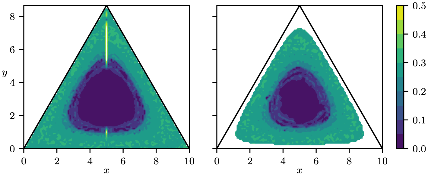
. Comparing the left and right plots in Figure 8 with the left plot of Figures 5(a) and 5(c), respectively, we conclude that tumbling motion, as identified by our classification in Section 4.1, is typically chaotic. In the left plot of Figure 8, a notable exception occurs for initial conditions lying on the vertical axis of symmetry, which remain on this axis with the given initial orientation. The periodic trajectories that occur on this axis of symmetry produce an unusually large value of the LLE in instances where they are highly unstable with respect to any perturbation away from the axis of symmetry. The same feature is not observed on the other two axes of symmetry as rounding errors prevent orbits from remaining on these axes. The inner region of both plots possesses a very small LLE. This is unsurprising given that vertical and central swinging motions mostly occur here and are periodic/quasi-periodic in nature. Wandering motion largely occurs over the regions where the LLE transitions from small to appreciable values. We note there are some interesting instances where small regions of insignificant LLE occur within the transition area and that these can be good places to look for unusual/exotic trajectories.
$\mathbf{e}=(0.5,0.5,-\sqrt{0.11})$
. Comparing the left and right plots in Figure 8 with the left plot of Figures 5(a) and 5(c), respectively, we conclude that tumbling motion, as identified by our classification in Section 4.1, is typically chaotic. In the left plot of Figure 8, a notable exception occurs for initial conditions lying on the vertical axis of symmetry, which remain on this axis with the given initial orientation. The periodic trajectories that occur on this axis of symmetry produce an unusually large value of the LLE in instances where they are highly unstable with respect to any perturbation away from the axis of symmetry. The same feature is not observed on the other two axes of symmetry as rounding errors prevent orbits from remaining on these axes. The inner region of both plots possesses a very small LLE. This is unsurprising given that vertical and central swinging motions mostly occur here and are periodic/quasi-periodic in nature. Wandering motion largely occurs over the regions where the LLE transitions from small to appreciable values. We note there are some interesting instances where small regions of insignificant LLE occur within the transition area and that these can be good places to look for unusual/exotic trajectories.
The largest Lyapunov exponent (LLE) of trajectories in the initial position $(x(0),y(0))$
plane with fixed initial orientations
$(x(0),y(0))$
plane with fixed initial orientations $\mathbf {e}(0)=(0,0,-1)$
(left) and
$\mathbf {e}(0)=(0,0,-1)$
(left) and $\mathbf {e}(0)=(0.8,0.5,-\sqrt {0.11})$
(right), with
$\mathbf {e}(0)=(0.8,0.5,-\sqrt {0.11})$
(right), with $U=10$
in each case. Darker (blue) regions indicate a smaller value of the exponent and are indicative of periodic or quasi-periodic motion. Lighter (green to yellow) regions indicate a larger value of the exponent and are indicative of chaotic motion. The right plot only shows the LLE for non-escaping orbits (that is, with locations producing an escaping orbit in white).
$U=10$
in each case. Darker (blue) regions indicate a smaller value of the exponent and are indicative of periodic or quasi-periodic motion. Lighter (green to yellow) regions indicate a larger value of the exponent and are indicative of chaotic motion. The right plot only shows the LLE for non-escaping orbits (that is, with locations producing an escaping orbit in white).
7 Conclusion
In this paper, we have investigated the dynamics associated with a simplified model of an active particle immersed in fluid flow through an equilateral triangular duct. Using a general Hamiltonian formulation associated with a broad class of point-like active particle models, we have described the equations of motion arising from the cubic Poiseuille field associated with steady laminar flow through an equilateral triangular duct. We then identified and analysed the stability of equilibrium points of the dynamical system. While the equilibrium points are similar in nature to those observed in previous studies featuring cylindrical and square cross-sections, that is, located at the centre of the cross-section and consisting of a centre for the upstream orientation and a saddle for the downstream orientation, orbits near the stable and unstable manifolds of the saddle equilibrium are somewhat distinctive in this case.
We adapted a classification scheme devised for rectangular cross-sections to the equilateral triangular duct geometry, essentially by considering how the procedure which examines the trace within the cross-section needed to be modified with respect to the symmetries of the triangular cross-section. Using this scheme, we show the existence of a diverse range of active particle motions, including central and vertical swinging, tumbling, off-centred trapping and wandering, which vary greatly depending on the value of U and the specific initial conditions. Given the parameter $U=10$
, a thorough exploration of initial condition space suggests the prominence of orbits, from most to least, is tumbling, escaping, wandering, vertical swinging, central swinging and off-centre trapping.
$U=10$
, a thorough exploration of initial condition space suggests the prominence of orbits, from most to least, is tumbling, escaping, wandering, vertical swinging, central swinging and off-centre trapping.
Although we had adapted the definition “vertical swinging” to account for swinging that might occur along any symmetry axis, our results lack the expected three-fold symmetry. The reason is that our computations are unable to produce orbits which remain exactly on the non-vertical axes of symmetry because it is impossible to exactly describe most points on these axes using the floating point arithmetic due to their irrational slope. It is unclear whether an alternative coordinate system exists that would facilitate the computation of orbits which remain on all three axes of symmetry.
It should be noted that the classification scheme used herein is not perfect. While it works well for values of U around $10$
, for significantly larger or smaller values of U, these classifications become less indicative of the quasi-periodic or chaotic nature of orbits. The classification scheme of Harding et al. [Reference Harding, Valani and Stokes9] works better in this respect, upon which further sub-classifications could be added. In addition, we showed the existence of some exotic orbits which are difficult to distinctly classify based on their trace within the cross-section alone. The (quasi-)periodic nature of exotic orbits may make it possible to use an estimate of the LLE to distinguish such orbits, but given such examples appear to be rare within the broader parameter space, it may not be worth increasing the complexity of our classification scheme to capture these. Small perturbations about the saddle equilibrium also produced distinct orbits that may warrant a distinct classification.
$10$
, for significantly larger or smaller values of U, these classifications become less indicative of the quasi-periodic or chaotic nature of orbits. The classification scheme of Harding et al. [Reference Harding, Valani and Stokes9] works better in this respect, upon which further sub-classifications could be added. In addition, we showed the existence of some exotic orbits which are difficult to distinctly classify based on their trace within the cross-section alone. The (quasi-)periodic nature of exotic orbits may make it possible to use an estimate of the LLE to distinguish such orbits, but given such examples appear to be rare within the broader parameter space, it may not be worth increasing the complexity of our classification scheme to capture these. Small perturbations about the saddle equilibrium also produced distinct orbits that may warrant a distinct classification.
We explored how changes in the fluid velocity and initial orientations affect on the dynamics of active particles, providing a broad collection of maps illustrating the variations in classification over parameter space. With smaller values of U, it is evident that escaping orbits become more prominent, largely at the expense of tumbling orbits. This is especially the case for initial orientations in the hemisphere around the downstream orientation ( $\mathbf {e}=+\mathbf {k}$
). This can be explained by the size of the basin as determined from the potential that arises from the Hamiltonian. A more complex model which accounted for wall collisions would significantly change the nature of such results. For larger U, although not shown, we expect an increase in the quantity of tumbling orbits, primarily at the expense of escaping and wandering orbits.
$\mathbf {e}=+\mathbf {k}$
). This can be explained by the size of the basin as determined from the potential that arises from the Hamiltonian. A more complex model which accounted for wall collisions would significantly change the nature of such results. For larger U, although not shown, we expect an increase in the quantity of tumbling orbits, primarily at the expense of escaping and wandering orbits.
We then examined the transitions between chaotic and (quasi-)periodic motion. Using Poincaré maps, we illustrate that larger values of $c_0$
are primarily associated with chaotic tumbling (or escaping) motions, while smaller values are primarily associated with quasi-periodic wandering and swinging motions. For the specific case
$c_0$
are primarily associated with chaotic tumbling (or escaping) motions, while smaller values are primarily associated with quasi-periodic wandering and swinging motions. For the specific case $U=10$
, our results illustrate that transition from primarily chaotic to primarily (quasi-)periodic motion occurs for values of
$U=10$
, our results illustrate that transition from primarily chaotic to primarily (quasi-)periodic motion occurs for values of $c_0$
over the range
$c_0$
over the range $+2-U/2=-3$
to
$+2-U/2=-3$
to $-U/2=-5$
. Furthermore, by calculating the LLE, we quantified the sensitivity to initial conditions over initial position space for two specific initial orientations with
$-U/2=-5$
. Furthermore, by calculating the LLE, we quantified the sensitivity to initial conditions over initial position space for two specific initial orientations with $U=10$
. These also affirm that chaotic motion is primarily associated with tumbling orbits.
$U=10$
. These also affirm that chaotic motion is primarily associated with tumbling orbits.
The broader findings have some qualitative overlap with what has been found previously within a square duct geometry. However, given the distinct symmetries of an equilateral triangular duct, many of the details are unique in nature. Identification of exotic orbits appears to be new. The simple cubic polynomial expression for Poiseuille flow through an equilateral triangular duct makes this a particularly efficient example for performing computations, especially when compared with using the series solution of Poiseuille flow for square ducts. In future work, we aim to investigate the effects of inertial lift on the dynamics of active particles within an equilateral triangular duct.
Acknowledgements
W. A. Truneh acknowledges the financial support provided by Wellington Doctoral Scholarship at Te Herenga Waka–Victoria University of Wellington.
















 Open access

