


1. Introduction
Flow past a circular cylinder is a canonical problem in fluid mechanics, which has been extensively studied for its theoretical significance and wide engineering applications, such as coastal canopies, offshore structures and subsea pipelines. A governing parameter for such flows is the Reynolds number ( $ \textit{Re} = \textit{UD}/\nu$
), where U is the free stream velocity, D is the cylinder diameter and ν is the kinematic viscosity. As Re increases, the wake transitions from a steady laminar flow through unsteady Hopf instability and three-dimensional (3-D) mode A and mode B instabilities to a chaotic and turbulent flow at Re ≳ 400 (Bloor Reference Bloor1963; Williamson Reference Williamson1996; Zdravkovich Reference Zdravkovich1997). A key phenomenon for the flow past a circular cylinder is the periodic (for laminar flows) or quasiperiodic (for turbulent flows) shedding of primary vortices in the wake of the cylinder, which affects not only the hydrodynamic forces on the cylinder but also turbulence characteristics, as well as associated heat transport, mixing and noise generation in the wake region.
$ \textit{Re} = \textit{UD}/\nu$
), where U is the free stream velocity, D is the cylinder diameter and ν is the kinematic viscosity. As Re increases, the wake transitions from a steady laminar flow through unsteady Hopf instability and three-dimensional (3-D) mode A and mode B instabilities to a chaotic and turbulent flow at Re ≳ 400 (Bloor Reference Bloor1963; Williamson Reference Williamson1996; Zdravkovich Reference Zdravkovich1997). A key phenomenon for the flow past a circular cylinder is the periodic (for laminar flows) or quasiperiodic (for turbulent flows) shedding of primary vortices in the wake of the cylinder, which affects not only the hydrodynamic forces on the cylinder but also turbulence characteristics, as well as associated heat transport, mixing and noise generation in the wake region.
Among various passive flow control strategies, the use of a rear-attached splitter plate has gained significant attention, owing to its geometric simplicity and effectiveness in modifying the vortex dynamics and hydrodynamic forces (Choi, Jeon & Kim Reference Choi, Jeon and Kim2008; Ran et al.
Reference Ran, Deng, Yu, Chen and Gao2023). Figure 1 illustrates an instantaneous 3-D turbulent wake behind a circular cylinder equipped with a splitter plate of non-dimensional length $ L/D$
= 1 at Re = 1000. The spanwise and streamwise vorticity components, ω
z
and ω
x
, are computed as
$ L/D$
= 1 at Re = 1000. The spanwise and streamwise vorticity components, ω
z
and ω
x
, are computed as
 \begin{align} \omega _{z} &=\left(\frac{\partial v}{\partial x}-\frac{\partial u}{\partial y}\right)\frac{D}{U}, \end{align}
 \begin{align} \omega _{x} &=\left(\frac{\partial w}{\partial y}-\frac{\partial v}{\partial z}\right)\frac{D}{U}, \end{align}
where $u$
,
$u$
, $v$
and
$v$
and $w$
are velocity components in the streamwise (x), transverse (y) and spanwise (z) directions, respectively. Compared with the 3-D wake behind an isolated circular cylinder reported by Jiang et al. (Reference Jiang, Hu, Cheng and Zhou2022), the presence of the splitter plate clearly shifts the vortex shedding farther downstream, which may then affect the hydrodynamic forces on the cylinder and turbulence characteristics in the wake.
$w$
are velocity components in the streamwise (x), transverse (y) and spanwise (z) directions, respectively. Compared with the 3-D wake behind an isolated circular cylinder reported by Jiang et al. (Reference Jiang, Hu, Cheng and Zhou2022), the presence of the splitter plate clearly shifts the vortex shedding farther downstream, which may then affect the hydrodynamic forces on the cylinder and turbulence characteristics in the wake.
As summarised in table 1, a large number of experimental and numerical studies have investigated the influence of a splitter plate on the hydrodynamic forces on the cylinder (such as the mean drag coefficient, fluctuating lift coefficient and vortex shedding frequency). Early experimental work by Roshko (Reference Roshko1954, Reference Roshko1961) found that at Re = 1.45 × 10⁴, the mean drag coefficient reduced significantly from 1.15 for an isolated cylinder to 0.72 for $ L/D$
= 5. Similar drag reduction behaviour was also widely reported in subsequent experimental studies listed in table 1. In addition, Apelt, West & Szewczyk (Reference Apelt, West and Szewczyk1973), Anderson & Szewczyk (Reference Anderson and Szewczyk1997) and Gao et al. (Reference Gao, Huang, Chen, Chen and Li2019) found that the drag reduction with increasing
$ L/D$
= 5. Similar drag reduction behaviour was also widely reported in subsequent experimental studies listed in table 1. In addition, Apelt, West & Szewczyk (Reference Apelt, West and Szewczyk1973), Anderson & Szewczyk (Reference Anderson and Szewczyk1997) and Gao et al. (Reference Gao, Huang, Chen, Chen and Li2019) found that the drag reduction with increasing $ L/D$
was nonlinear – a significant drag reduction up to ∼30 % was achieved by increasing
$ L/D$
was nonlinear – a significant drag reduction up to ∼30 % was achieved by increasing $ L/D$
from 0 to ∼1, but further increase in
$ L/D$
from 0 to ∼1, but further increase in $ L/D$
beyond 1 resulted in minimal improvement in the drag reduction. For the fluctuating lift coefficient, a maximum reduction up to ∼80 % was achieved by increasing
$ L/D$
beyond 1 resulted in minimal improvement in the drag reduction. For the fluctuating lift coefficient, a maximum reduction up to ∼80 % was achieved by increasing $ L/D$
from 0 to ∼1, but further increase in
$ L/D$
from 0 to ∼1, but further increase in $ L/D$
beyond 1 led to diminished lift reduction (Gao et al.
Reference Gao, Huang, Chen, Chen and Li2019). These nonlinear variations in the hydrodynamic coefficients with
$ L/D$
beyond 1 led to diminished lift reduction (Gao et al.
Reference Gao, Huang, Chen, Chen and Li2019). These nonlinear variations in the hydrodynamic coefficients with $ L/D$
were also observed numerically by two-dimensional (2-D) (Kwon & Choi Reference Kwon and Choi1996; Vu, Ahn & Hwang Reference Vu, Ahn and Hwang2016) and 3-D direct numerical simulations (DNS) (de Araujo, Schettini & Silvestrini Reference de Araujo, Schettini and Silvestrini2018; Jiang Reference Jiang2025) at relatively low Re of ∼102–103. Collectively, these findings suggest that while a splitter plate is effective in controlling the hydrodynamic forces on the cylinder, the control effect is highly sensitive to the plate length, and an optimal control is often achieved at
$ L/D$
were also observed numerically by two-dimensional (2-D) (Kwon & Choi Reference Kwon and Choi1996; Vu, Ahn & Hwang Reference Vu, Ahn and Hwang2016) and 3-D direct numerical simulations (DNS) (de Araujo, Schettini & Silvestrini Reference de Araujo, Schettini and Silvestrini2018; Jiang Reference Jiang2025) at relatively low Re of ∼102–103. Collectively, these findings suggest that while a splitter plate is effective in controlling the hydrodynamic forces on the cylinder, the control effect is highly sensitive to the plate length, and an optimal control is often achieved at $ L/D$
∼ 1.
$ L/D$
∼ 1.
Summary of experimental and numerical studies on flow past a circular cylinder with a rear-attached splitter plate.

Instantaneous vorticity field for a circular cylinder with a splitter plate ( $ L/D$
= 1) at Re = 1000: (a) isosurfaces of ω
z
(translucent) and ω
x
(opaque); (b) isosurfaces of ω
z
only; (c) isosurfaces of ω
x
only. The red and blue isosurfaces correspond to positive and negative vorticity values of ±4, respectively.
$ L/D$
= 1) at Re = 1000: (a) isosurfaces of ω
z
(translucent) and ω
x
(opaque); (b) isosurfaces of ω
z
only; (c) isosurfaces of ω
x
only. The red and blue isosurfaces correspond to positive and negative vorticity values of ±4, respectively.

From a mechanistic perspective, Gerrard (Reference Gerrard1966) proposed that vortex shedding is governed by a circulation ‘feed-and-cutoff’ process within the formation region. A growing vortex is continuously fed by the separating shear layer until it becomes sufficiently strong to draw opposite-signed vorticity across the wake, thereby cutting off further supply and triggering shedding. Gerrard (Reference Gerrard1966) further argued that a rear-attached splitter plate can suppress this cross-wake interaction and effectively extend the vortex formation region, which tends to delay roll-up and reduce the shedding frequency. Building upon this framework, Anderson & Szewczyk (Reference Anderson and Szewczyk1997) found that the shedding frequency exhibits a non-monotonic dependence on plate length (over $ L/D$
= 0–1.5) because of the different interaction modes between the upper and lower shear layers. Apelt & West (Reference Apelt and West1975) extended experimental investigations to longer
$ L/D$
= 0–1.5) because of the different interaction modes between the upper and lower shear layers. Apelt & West (Reference Apelt and West1975) extended experimental investigations to longer $ L/D$
(= 2–7) and reported that the influence of
$ L/D$
(= 2–7) and reported that the influence of $ L/D$
eventually saturates. Specifically, the drag coefficient and shedding frequency change with
$ L/D$
eventually saturates. Specifically, the drag coefficient and shedding frequency change with $ L/D$
only up to approximately
$ L/D$
only up to approximately $ L/D$
≈ 5, beyond which no further significant variation occurs. Importantly, they also observed that although regular vortex shedding from the cylinder can be eliminated for sufficiently long plates, a well-formed vortex street may still develop farther downstream.
$ L/D$
≈ 5, beyond which no further significant variation occurs. Importantly, they also observed that although regular vortex shedding from the cylinder can be eliminated for sufficiently long plates, a well-formed vortex street may still develop farther downstream.
Overall, previous studies have established that the splitter plate may alter shear-layer development and transverse shear-layer oscillations, thereby altering vortex shedding frequency, particularly for relatively short plates ( $ L/D$
< 1.5). However, the underlying physical mechanism for the optimal control observed at
$ L/D$
< 1.5). However, the underlying physical mechanism for the optimal control observed at $ L/D$
∼ 1 has not been explained in previous studies.
$ L/D$
∼ 1 has not been explained in previous studies.
In contrast to the extensive investigation on the influence of a splitter plate on the hydrodynamic forces, little attention has been paid to the turbulence characteristics in the wake. To the best knowledge of the authors, only Duan & Wang (Reference Duan and Wang2021) and Zhou et al. (Reference Zhou, Qiu, Li, Wang, Zhou and Liu2024) presented evidence for the control of the turbulent kinetic energy (TKE) in the near wake by a splitter plate based on particle image velocimetry measurements of the velocity variances in the near-wake region. Specifically, Duan & Wang (Reference Duan and Wang2021) performed wind-tunnel experiments at Re = 3.83 × 10⁴–9.57 × 10⁴ and $ L/D$
= 0 and 1, and found that the TKE at
$ L/D$
= 0 and 1, and found that the TKE at $ L/D$
= 1 was noticeably smaller than that at
$ L/D$
= 1 was noticeably smaller than that at $ L/D$
= 0. Zhou et al. (Reference Zhou, Qiu, Li, Wang, Zhou and Liu2024) performed flume experiments at Re = 3900 and
$ L/D$
= 0. Zhou et al. (Reference Zhou, Qiu, Li, Wang, Zhou and Liu2024) performed flume experiments at Re = 3900 and $ L/D$
= 0–2, and found that the TKE decreased significantly with increasing
$ L/D$
= 0–2, and found that the TKE decreased significantly with increasing $ L/D$
. Although Duan & Wang (Reference Duan and Wang2021) and Zhou et al. (Reference Zhou, Qiu, Li, Wang, Zhou and Liu2024) revealed effectiveness of the splitter plate in controlling the TKE in the wake, there remains certain limitations and unanswered questions.
$ L/D$
. Although Duan & Wang (Reference Duan and Wang2021) and Zhou et al. (Reference Zhou, Qiu, Li, Wang, Zhou and Liu2024) revealed effectiveness of the splitter plate in controlling the TKE in the wake, there remains certain limitations and unanswered questions.
-
(i) The particle image velocimetry measurements by Duan & Wang (Reference Duan and Wang2021) and Zhou et al. (Reference Zhou, Qiu, Li, Wang, Zhou and Liu2024) only captured the planar (streamwise and transverse) TKE components, while the spanwise component was not measured, such that the reported TKE was incomplete.
-
(ii) Although variations in the hydrodynamic and turbulence characteristics are both tied to the variation in the vortex dynamics, the variation trend of the planar TKE with $ L/D$
(with a monotonic reduction) is surprisingly different to the variation trend of the hydrodynamic forces with
$ L/D$
(with an optimal control at
$ L/D$
∼ 1). Because the control effect on the TKE is much less studied than that on the hydrodynamic forces, it is worthwhile to re-examine the effect of
$ L/D$
on the TKE in detail. Indeed, this study identifies a non-monotonic reduction in the TKE with
$ L/D$
, where a local minimum in the TKE is observed at
$ L/D$
∼ 1.5, and corresponding physical mechanisms are unveiled to support this new finding.
$ L/D$
(with a monotonic reduction) is surprisingly different to the variation trend of the hydrodynamic forces with
$ L/D$
(with an optimal control at
$ L/D$
∼ 1). Because the control effect on the TKE is much less studied than that on the hydrodynamic forces, it is worthwhile to re-examine the effect of
$ L/D$
on the TKE in detail. Indeed, this study identifies a non-monotonic reduction in the TKE with
$ L/D$
, where a local minimum in the TKE is observed at
$ L/D$
∼ 1.5, and corresponding physical mechanisms are unveiled to support this new finding. -
(iii) Other than the TKE, the control effects of a splitter plate on other turbulence characteristics, such as the kinetic energy dissipation rate and the spatial distribution of the turbulence (e.g. degree of isotropy and homogeneity of turbulence) remain to be explored.


To address these limitations and questions, this study will examine in detail the effect of a splitter plate on the vortex dynamics and turbulence characteristics in the wake of a circular cylinder at a turbulent Re of 1000 and $ L/D$
= 0–4. To circumvent experimental difficulties in quantifying the spanwise component of TKE (Duan & Wang Reference Duan and Wang2021; Zhou et al.
Reference Zhou, Qiu, Li, Wang, Zhou and Liu2024) and the kinetic energy dissipation rate (Chen et al.
Reference Chen, Zhou, Antonia and Zhou2018), high-fidelity 3-D DNS are performed in this study to resolve full turbulence characteristics. The present findings at Re = 1000 are expected to be applicable to a range of Reynolds numbers, as good qualitative agreements have been observed in the Kolmogorov length scales and velocity derivative terms constituting the kinetic energy dissipation rate in a cylinder wake at Re = 1000 (Jiang et al.
Reference Jiang, Hu, Cheng and Zhou2022) and Re = 2500 (Chen et al.
Reference Chen, Zhou, Antonia and Zhou2018), and in the spatiotemporal evolution of the primary vortices in a cylinder wake at Re = 1000 (Jiang et al.
Reference Jiang, Hu, Cheng and Zhou2022), Re = 2540 (Zhou et al.
Reference Zhou, Zhou, Yiu and Chua2003) and Re = 5800 (Zhou, Zhang & Yiu Reference Zhou, Zhang and Yiu2002). From a practical standpoint, the splitter plate length cannot be increased indefinitely due to constraints such as material usage, structural strength/stiffness and installation considerations. Motivated by both these practical constraints and the saturation/critical length observed by Apelt & West (Reference Apelt and West1975), the present study focuses on
$ L/D$
= 0–4. To circumvent experimental difficulties in quantifying the spanwise component of TKE (Duan & Wang Reference Duan and Wang2021; Zhou et al.
Reference Zhou, Qiu, Li, Wang, Zhou and Liu2024) and the kinetic energy dissipation rate (Chen et al.
Reference Chen, Zhou, Antonia and Zhou2018), high-fidelity 3-D DNS are performed in this study to resolve full turbulence characteristics. The present findings at Re = 1000 are expected to be applicable to a range of Reynolds numbers, as good qualitative agreements have been observed in the Kolmogorov length scales and velocity derivative terms constituting the kinetic energy dissipation rate in a cylinder wake at Re = 1000 (Jiang et al.
Reference Jiang, Hu, Cheng and Zhou2022) and Re = 2500 (Chen et al.
Reference Chen, Zhou, Antonia and Zhou2018), and in the spatiotemporal evolution of the primary vortices in a cylinder wake at Re = 1000 (Jiang et al.
Reference Jiang, Hu, Cheng and Zhou2022), Re = 2540 (Zhou et al.
Reference Zhou, Zhou, Yiu and Chua2003) and Re = 5800 (Zhou, Zhang & Yiu Reference Zhou, Zhang and Yiu2002). From a practical standpoint, the splitter plate length cannot be increased indefinitely due to constraints such as material usage, structural strength/stiffness and installation considerations. Motivated by both these practical constraints and the saturation/critical length observed by Apelt & West (Reference Apelt and West1975), the present study focuses on $ L/D$
= 0–4.
$ L/D$
= 0–4.
2. Numerical model
2.1. Numerical method
The present 3-D DNS were conducted by solving the continuity equation and incompressible Navier–Stokes equations for the flow past a circular cylinder with a rear-attached splitter plate. The governing equations are expressed as
 \begin{align} \frac{\partial u_{i}}{\partial x_{i}} &=0, \end{align}
 \begin{align} \frac{\partial u_{i}}{\partial t}+u_{\kern-1pt j}\frac{\partial u_{i}}{\partial x_{\kern-1pt j}} &=-\frac{\partial p}{\partial x_{i}}+\nu \frac{\partial ^{2}u_{i}}{\partial x_{\kern-1pt j}\partial x_{i}}, \end{align}
where u i denotes the velocity component in the direction x i , p is the kinematic pressure, t is time and ν is the kinematic viscosity.
To solve (2.1) and (2.2), the open-source spectral/hp element framework Nektar++ (Cantwell, Moxey & Comerford Reference Cantwell2015) was employed. The simulations followed a quasi-3-D formulation, where the x–y plane was discretised using high-order spectral/hp elements (Karniadakis & Sherwin Reference Karniadakis and Sherwin2005), while the spanwise z-direction was treated by Fourier decomposition (Karniadakis Reference Karniadakis1990). This hybrid approach takes advantage of both spectral accuracy and computational efficiency, offering significant benefits over traditional finite volume or other similar methods (Cantwell et al. Reference Cantwell2015; Moxey et al. Reference Moxey2020; Jiang & Cheng Reference Jiang and Cheng2021).
A second-order implicit–explicit time integration scheme was employed, where the linear viscous terms were treated implicitly and the nonlinear convective terms explicitly (Karniadakis, Israeli & Orszag Reference Karniadakis, Israeli and Orszag1991; Cantwell et al. Reference Cantwell2015). To enhance numerical stability and computational efficiency, a velocity correction scheme was incorporated (Karniadakis et al. Reference Karniadakis, Israeli and Orszag1991). Additionally, the spectral vanishing viscosity (SVV) technique was used to stabilise the numerical solution at relatively large Re (Kirby & Sherwin Reference Kirby and Sherwin2006). The SVV cutoff ratio and diffusion coefficient were set to 0.9 and 0.1, respectively, which were consistent with those used by Jiang et al. (Reference Jiang, Hu, Cheng and Zhou2022) for flow past an isolated circular cylinder at Re = 1000. Jiang et al. (Reference Jiang, Hu, Cheng and Zhou2022) demonstrated that a further reduction in the SVV diffusion coefficient from 0.1 to 0.05 resulted in minimal influence on the kinetic energy dissipation rate in the wake, and this conclusion was further supported by the SVV sensitivity analysis presented in § 2.3 for the present splitter-plate configuration.
2.2. Computational domain and mesh
The computational domain for the present 3-D DNS is illustrated in figure 2(a). The cylinder was centred at ( $ x/D$
,
$ x/D$
, $ y/D$
) = (0, 0), with its axis aligned parallel to the z-direction. The distances from the cylinder centre to the top and bottom boundaries, the inlet, and the outlet were 30D, 30D and 40D, respectively. The splitter plate was attached to the rear end of the cylinder as a thin, zero-thickness plate. While the plate thickness was a geometric parameter that may affect the results to a small extent (Jiang Reference Jiang2025), in this study an idealised zero-thickness splitter plate was examined, so as to isolate the primary effect of
$ y/D$
) = (0, 0), with its axis aligned parallel to the z-direction. The distances from the cylinder centre to the top and bottom boundaries, the inlet, and the outlet were 30D, 30D and 40D, respectively. The splitter plate was attached to the rear end of the cylinder as a thin, zero-thickness plate. While the plate thickness was a geometric parameter that may affect the results to a small extent (Jiang Reference Jiang2025), in this study an idealised zero-thickness splitter plate was examined, so as to isolate the primary effect of $ L/D$
and to keep the parameter space tractable. The spanwise domain length was 6D. The boundary conditions applied at each boundary are summarised in table 2.
$ L/D$
and to keep the parameter space tractable. The spanwise domain length was 6D. The boundary conditions applied at each boundary are summarised in table 2.
Boundary conditions for the present 3-D DNS.

(a) Computational domain (not to scale) and (b) macroelement mesh near the circular cylinder with a rear-attached splitter plate of $ L/D$
= 2. The blue line represents the splitter plate.
$ L/D$
= 2. The blue line represents the splitter plate.

In the x–y plane, the perimeter of the cylinder was discretised into 64 macroelements. The height of the first macroelement layer adjacent to the cylinder surface was 0.0055D. At the trailing edge of the splitter plate, the macroelement resolution was 0.0667D × 0.0288D. To adequately capture the turbulence scales in the wake region, the streamwise size of the macroelements was maintained at Δ $ x/D$
= 0.2 in the region
$ x/D$
= 0.2 in the region $ x/D$
= (
$ x/D$
= ( $ L/D$
+ 1) to 30. For all
$ L/D$
+ 1) to 30. For all $ L/D$
conditions, the total number of macroelements in the x–y plane was approximately 14 000. Each macroelement was further expanded using a fourth-order Lagrange polynomials (denoted N
p
= 4). Figure 2(b) illustrates the macroelement mesh near the cylinder for the case
$ L/D$
conditions, the total number of macroelements in the x–y plane was approximately 14 000. Each macroelement was further expanded using a fourth-order Lagrange polynomials (denoted N
p
= 4). Figure 2(b) illustrates the macroelement mesh near the cylinder for the case $ L/D$
= 2. The spanwise direction of the computational domain was discretised using 128 Fourier planes across a domain length
$ L/D$
= 2. The spanwise direction of the computational domain was discretised using 128 Fourier planes across a domain length $ L_{z}/D$
= 6.
$ L_{z}/D$
= 6.
Each simulation was initiated using an impulsive start. A non-dimensional time step size ( $ \Delta t^{*} = \Delta \textit{tU}/D$
) of 0.0025 was adopted, which corresponded to a Courant–Friedrichs–Lewy number below 0.5. Each case was simulated for a non-dimensional duration of at least 1000 time units (t*
= tU/D), within which statistical analysis was performed over a period of no less than 600 non-dimensional time units. The sampling frequency for the statistical data was Δt*
.
$ \Delta t^{*} = \Delta \textit{tU}/D$
) of 0.0025 was adopted, which corresponded to a Courant–Friedrichs–Lewy number below 0.5. Each case was simulated for a non-dimensional duration of at least 1000 time units (t*
= tU/D), within which statistical analysis was performed over a period of no less than 600 non-dimensional time units. The sampling frequency for the statistical data was Δt*
.
Mesh dependence check for $ L/D$
= 2. The relative differences for variation cases 1 to 6 are calculated with respect to the reference case and are shown in the parentheses.
$ L/D$
= 2. The relative differences for variation cases 1 to 6 are calculated with respect to the reference case and are shown in the parentheses.

2.3. Mesh dependence study
The reference mesh described in § 2.2 used N
p
= 4, $ L_{z}/D$
= 6 and 128 Fourier planes. This mesh resolution was previously verified by Jiang et al. (Reference Jiang, Hu, Cheng and Zhou2022) for the case of an isolated circular cylinder at Re = 1000, who demonstrated sufficient accuracy in capturing the wake dynamics and turbulence characteristics. In this study, the adequacy of the reference mesh was further confirmed by a case with the splitter plate. Specifically, a 3-D mesh dependence study was conducted for the case
$ L_{z}/D$
= 6 and 128 Fourier planes. This mesh resolution was previously verified by Jiang et al. (Reference Jiang, Hu, Cheng and Zhou2022) for the case of an isolated circular cylinder at Re = 1000, who demonstrated sufficient accuracy in capturing the wake dynamics and turbulence characteristics. In this study, the adequacy of the reference mesh was further confirmed by a case with the splitter plate. Specifically, a 3-D mesh dependence study was conducted for the case $ L/D$
= 2, where several variations to the reference mesh were considered.
$ L/D$
= 2, where several variations to the reference mesh were considered.
-
(i) Variation case 1. The
$ L_{z}/D$
was unchanged, while the number of Fourier planes was increased from 128 to 256 (such that the spanwise mesh resolution was doubled). -
(ii) Variation case 2. The
$ L_{z}/D$
was extended from 6 to 12, and the number of Fourier planes was also increased from 128 to 256 (such that the spanwise mesh resolution was unchanged). -
(iii) Variation case 3. The polynomial order N p was increased from 4 to 5.
-
(iv) Variation case 4. The polynomial order N p was increased from 4 to 6.
-
(v) Variation case 5. The number of grids in the x- and y-directions were both increased by a factor of 1.25, and the total number of macroelements in the x–y plane reached 1.252 times that of the reference case.
-
(vi) Variation case 6. the SVV diffusion coefficient was reduced from 0.1 to 0.05.


Table 3 summarises the numerical results of these cases. The Strouhal number (St), drag coefficient (C D ) and lift coefficient (C L ) are defined as follows:
 \begin{align} St &=\frac{f_{L}D}{U}, \end{align}
 \begin{align} C_{D} &=\frac{F_{D}}{\tfrac{1}{2}\rho U^{2}D}, \end{align}
 \begin{align} C_{L} &=\frac{F_{L}}{\tfrac{1}{2}\rho U^{2}D}, \end{align}
where F
D
and F
L
represent the drag and lift forces per unit spanwise length, respectively. The value f
L
is the dominant vortex shedding frequency extracted from the lift force using a fast Fourier transform (FFT). The time-averaged drag coefficient is denoted $\overline{\textit{C}_{\textit{D}}}$
. The root-mean-square lift coefficient is expressed as
$\overline{\textit{C}_{\textit{D}}}$
. The root-mean-square lift coefficient is expressed as
 \begin{equation} C^{\prime}_{L}=\sqrt{\frac{1}{N}{\sum }_{i=1}^{N}\left(C_{L,i}-\overline{C_{L}}\right)^{2}}, \end{equation}
where N represents the number of samples. For the cases involving a splitter plate, the hydrodynamic forces on the cylinder and splitter plate are evaluated separately, with the corresponding coefficients labelled by the subscripts ‘cyl’ and ‘plate’, respectively.
As shown in table 3, the St and $\overline{\textit{C}_{\textit{D},\textit{cyl}}}$
values for the variation cases 1–6 displayed less than 1 % difference to those of the reference case. Except for the variation case 2, the C
′
L
on both the cylinder and the splitter plate also displayed little difference to those of the reference case. For the variation case 2, a noticeable reduction in C
′
L
was observed on both the cylinder and the splitter plate, which was physically attributed to increased spanwise phase cancellation as the spanwise domain length increased (Henderson Reference Henderson1997) and was not induced by numerical aspects. Although the spanwise domain length L
z
had a significant effect on the root-mean-square quantities such as C
′
L
(Jiang, Cheng & An Reference Jiang, Cheng and An2017), it had negligible influence on the time-averaged quantities (Jiang & Cheng Reference Jiang and Cheng2021). Therefore, the time- and spanwise-averaged turbulence characteristics examined in this study were not noticeably affected by L
z
.
$\overline{\textit{C}_{\textit{D},\textit{cyl}}}$
values for the variation cases 1–6 displayed less than 1 % difference to those of the reference case. Except for the variation case 2, the C
′
L
on both the cylinder and the splitter plate also displayed little difference to those of the reference case. For the variation case 2, a noticeable reduction in C
′
L
was observed on both the cylinder and the splitter plate, which was physically attributed to increased spanwise phase cancellation as the spanwise domain length increased (Henderson Reference Henderson1997) and was not induced by numerical aspects. Although the spanwise domain length L
z
had a significant effect on the root-mean-square quantities such as C
′
L
(Jiang, Cheng & An Reference Jiang, Cheng and An2017), it had negligible influence on the time-averaged quantities (Jiang & Cheng Reference Jiang and Cheng2021). Therefore, the time- and spanwise-averaged turbulence characteristics examined in this study were not noticeably affected by L
z
.
Time- and span-averaged velocity profiles at streamwise locations $ x/D$
= 0, 1, 2, 3, 4 and 5: (a)
$ x/D$
= 0, 1, 2, 3, 4 and 5: (a) $\overline{\textit{u}_{\textit{x}}}/U$
for variation cases 1–3, (b)
$\overline{\textit{u}_{\textit{x}}}/U$
for variation cases 1–3, (b) $\overline{\textit{u}_{\textit{y}}}/U$
for variation cases 1–3, (c)
$\overline{\textit{u}_{\textit{y}}}/U$
for variation cases 1–3, (c) $\overline{\textit{u}_{\textit{x}}}$
/U for variation cases 4–6 and (d)
$\overline{\textit{u}_{\textit{x}}}$
/U for variation cases 4–6 and (d) $\overline{\textit{u}_{\textit{y}}}$
/U for variation cases 4–6. Different line types represent different cases, and different colours represent different
$\overline{\textit{u}_{\textit{y}}}$
/U for variation cases 4–6. Different line types represent different cases, and different colours represent different $ x/D$
values.
$ x/D$
values.

To further investigate the sensitivity of the computational domain and mesh, figure 3 shows the time- and span-averaged velocity profiles at $ x/D$
= 0, 1, 2, 3, 4 and 5 for the cases listed in table 3. As illustrated in figure 3, the time- and span-averaged streamwise velocity (
$ x/D$
= 0, 1, 2, 3, 4 and 5 for the cases listed in table 3. As illustrated in figure 3, the time- and span-averaged streamwise velocity ( $\overline{\textit{u}_{\textit{x}}}$
) and transverse velocity (
$\overline{\textit{u}_{\textit{x}}}$
) and transverse velocity ( $\overline{\textit{u}_{\textit{y}}}$
) profiles obtained by the seven cases exhibited excellent agreement. This indicated that the reference case was sufficient to capture the wake dynamics and was therefore adopted for the present DNS.
$\overline{\textit{u}_{\textit{y}}}$
) profiles obtained by the seven cases exhibited excellent agreement. This indicated that the reference case was sufficient to capture the wake dynamics and was therefore adopted for the present DNS.
To assess the sensitivity of the results to the SVV diffusion coefficient, an additional case (variation case 6) was performed by reducing the SVV diffusion coefficient from 0.1 to 0.05. In addition to showing good agreement with the reference case in table 3 regarding the hydrodynamic forces, figure 4 shows transverse distribution of the mean dissipation rate at $ x/D$
= 10 and 20 for the two SVV settings. The results suggested that halving the SVV diffusion coefficient resulted in negligible changes in the dissipation rate. Therefore, the SVV diffusion coefficient of 0.1 was adopted in the present study.
$ x/D$
= 10 and 20 for the two SVV settings. The results suggested that halving the SVV diffusion coefficient resulted in negligible changes in the dissipation rate. Therefore, the SVV diffusion coefficient of 0.1 was adopted in the present study.
Transverse distribution of the mean kinetic energy dissipation rate at (a) $ x/D$
= 10 and (b)
$ x/D$
= 10 and (b) $ x/D$
= 20, based on different SVV diffusion coefficients.
$ x/D$
= 20, based on different SVV diffusion coefficients.

To verify whether the wake resolution was sufficient to capture the turbulence scales, Kolmogorov-scale normalised quantities were examined. The Kolmogorov time scale (τη ) and length scale (η) are calculated as
 \begin{align} \tau _{\eta } &=\left(\frac{\nu }{\varepsilon }\right)^{1/2}, \end{align}
 \begin{align} \eta &=\left(\frac{\nu ^{3}}{\varepsilon }\right)^{1/4}. \end{align}
Figure 5(a,b) presented the Kolmogorov time scale (τ
η
) and length scale (η) along both $ y/D$
= 0 (the wake centreline) and
$ y/D$
= 0 (the wake centreline) and $ y/D$
= 0.512 (a macroelement centre). At
$ y/D$
= 0.512 (a macroelement centre). At $ y/D$
= 0, the minimum τ
η
occurred near the end of the splitter plate and reached approximately 0.055, which was still significantly larger than the time step size used in the simulation (Δt
* = 0.0025). At all other locations, τ
η
was even larger, confirming that the temporal resolution was sufficient to capture the time evolution of turbulence in the wake. Figures 5(c) and 5(d) present the ratio between the cell size and η along
$ y/D$
= 0, the minimum τ
η
occurred near the end of the splitter plate and reached approximately 0.055, which was still significantly larger than the time step size used in the simulation (Δt
* = 0.0025). At all other locations, τ
η
was even larger, confirming that the temporal resolution was sufficient to capture the time evolution of turbulence in the wake. Figures 5(c) and 5(d) present the ratio between the cell size and η along $ y/D$
= 0 and 0.512, respectively. These ratios are presented for the streamwise (Δx), transverse (Δy) and spanwise (Δz) directions. Notably, since the macroelement mesh in the x–y plane was further refined using p-type spectral expansion, the effective resolution in these directions was obtained by dividing the macroelement size by the polynomial order N
p
. Across the entire wake region, the normalised cell sizes remained below 6 (and mostly below 3). These values were consistent with the widely used DNS resolution criterion, where the smallest resolved length scale should be several times the Kolmogorov length scale η (Moin & Mahesh Reference Moin and Mahesh1998; Laizet, Nedić & Vassilicos Reference Laizet, Nedić and Vassilicos2015; Song et al.
Reference Song, Ping, Zhu, Zhou, Bao, Cao and Han2022; Lu et al.
Reference Lu, Aljubaili, Zahtila, Chan and Ooi2023).
$ y/D$
= 0 and 0.512, respectively. These ratios are presented for the streamwise (Δx), transverse (Δy) and spanwise (Δz) directions. Notably, since the macroelement mesh in the x–y plane was further refined using p-type spectral expansion, the effective resolution in these directions was obtained by dividing the macroelement size by the polynomial order N
p
. Across the entire wake region, the normalised cell sizes remained below 6 (and mostly below 3). These values were consistent with the widely used DNS resolution criterion, where the smallest resolved length scale should be several times the Kolmogorov length scale η (Moin & Mahesh Reference Moin and Mahesh1998; Laizet, Nedić & Vassilicos Reference Laizet, Nedić and Vassilicos2015; Song et al.
Reference Song, Ping, Zhu, Zhou, Bao, Cao and Han2022; Lu et al.
Reference Lu, Aljubaili, Zahtila, Chan and Ooi2023).
Streamwise variation of the Kolmogorov scales for the case $ L/D$
= 2: (a) Kolmogorov time scale τ
η
; (b) Kolmogorov length scale η; (c) cell size to η at
$ L/D$
= 2: (a) Kolmogorov time scale τ
η
; (b) Kolmogorov length scale η; (c) cell size to η at $ y/D$
= 0; (d) cell size to η at
$ y/D$
= 0; (d) cell size to η at $ y/D$
= 0.512.
$ y/D$
= 0.512.

2.4. Phase-averaging technique
To isolate and analyse the coherent structures in the wake, a phase-averaging technique is employed, which follows the approach used by Jiang et al. (Reference Jiang, Hu, Cheng and Zhou2022). Compared with the classical phase-averaging technique used in prior wind-tunnel experiments, which were based on measurement of velocity signals at discrete locations (Matsumura & Antonia Reference Matsumura and Antonia1993; Zhou et al. Reference Zhou, Zhang and Yiu2002; Chen et al. Reference Chen, Zhou, Antonia and Zhou2018), the present method leverages a large volume of instantaneous flow fields obtained from the numerical simulation, which enables a direct presentation of the flow field contours.
For each simulation case, the transverse velocity $v$
sampled at a specific streamwise location (
$v$
sampled at a specific streamwise location ( $ x/D$
= 5, 10 and 20) and
$ x/D$
= 5, 10 and 20) and $ y/D$
= 1 is used as a reference signal for phase average at this
$ y/D$
= 1 is used as a reference signal for phase average at this $ x/D$
location. To enhance statistical convergence, reference signals are taken at four equally spaced spanwise locations (
$ x/D$
location. To enhance statistical convergence, reference signals are taken at four equally spaced spanwise locations ( $ z/D$
= 0, 1.5, 3 and 4.5), with each being processed individually. The reference
$ z/D$
= 0, 1.5, 3 and 4.5), with each being processed individually. The reference $v$
signal is then filtered using a fourth-order Butterworth filter centred at the vortex shedding frequency (e.g. Zhou et al.
Reference Zhou, Zhang and Yiu2002; Chen et al.
Reference Chen, Zhou, Antonia and Zhou2018). Figure 6(a) shows an example of the
$v$
signal is then filtered using a fourth-order Butterworth filter centred at the vortex shedding frequency (e.g. Zhou et al.
Reference Zhou, Zhang and Yiu2002; Chen et al.
Reference Chen, Zhou, Antonia and Zhou2018). Figure 6(a) shows an example of the $v$
signal sampled at (
$v$
signal sampled at ( $ x/D$
,
$ x/D$
, $ y/D$
,
$ y/D$
, $ z/D$
) = (10, 1, 3) and the filtered signal. Based on the filtered signal, the local peaks and troughs are identified and assigned phase values φ = 0 and φ = π, respectively. Each vortex shedding period T (from peak to peak) is then equally divided into 16 phase intervals. The instantaneous flow fields corresponding to each phase value are collected over 100T and averaged to obtain the phase-averaged field 〈u〉
p
, where p denotes the phase index. The final phase-averaged field is obtained by averaging the results from the four spanwise locations. The sampling interval of T/16 and sampling duration of 100T (together with the use of four spanwise locations) were demonstrated to be sufficient for phase-averaged turbulence analysis by Jiang et al. (Reference Jiang, Hu, Cheng and Zhou2022).
$ z/D$
) = (10, 1, 3) and the filtered signal. Based on the filtered signal, the local peaks and troughs are identified and assigned phase values φ = 0 and φ = π, respectively. Each vortex shedding period T (from peak to peak) is then equally divided into 16 phase intervals. The instantaneous flow fields corresponding to each phase value are collected over 100T and averaged to obtain the phase-averaged field 〈u〉
p
, where p denotes the phase index. The final phase-averaged field is obtained by averaging the results from the four spanwise locations. The sampling interval of T/16 and sampling duration of 100T (together with the use of four spanwise locations) were demonstrated to be sufficient for phase-averaged turbulence analysis by Jiang et al. (Reference Jiang, Hu, Cheng and Zhou2022).
Reference signals used for phase-averaging for the case $ L/D$
= 2: (a) the
$ L/D$
= 2: (a) the $v$
signal sampled at (
$v$
signal sampled at ( $ x/D$
,
$ x/D$
, $ y/D$
,
$ y/D$
, $ z/D$
) = (10, 1, 3) and its bandpass-filtered counterpart, and (b) the C
L
on the cylinder. The filtered signal in (a) is scaled by a factor of 5.06779 to match the standard deviation of the original signal while preserving the phase.
$ z/D$
) = (10, 1, 3) and its bandpass-filtered counterpart, and (b) the C
L
on the cylinder. The filtered signal in (a) is scaled by a factor of 5.06779 to match the standard deviation of the original signal while preserving the phase.

Eventually, the coherent velocity component ( $\tilde{\textit{u}}_{\textit{p}}$
) at each phase is defined as the difference between the phase-averaged velocity (〈u〉
p
) and the time- and span-averaged mean velocity (u
m
),
$\tilde{\textit{u}}_{\textit{p}}$
) at each phase is defined as the difference between the phase-averaged velocity (〈u〉
p
) and the time- and span-averaged mean velocity (u
m
),
 \begin{equation}\tilde{{u}}_{\textit{p}} = \left\langle {u}\right\rangle _{\textit{p}}-{u}_{\textit{m}}.\end{equation}
Similarly, to extract coherent structures very close to the cylinder, the lift coefficient C L on the cylinder is also used as a reference signal without filtering, owing to its smooth temporal variation (figure 6b ).
3. Primary vortex street in the wake
3.1. Formation and shedding of the primary vortices
A splitter plate attached to the rear end of the circular cylinder may significantly alter the vortex dynamics and thus turbulence characteristics in the wake region. Because the present study considers the turbulent wake at Re = 1000, where the vortex shedding and vortex street are quasiperiodic, phase averaging is performed. In this section, the focus is on the vortex formation and shedding that occur in the immediate near wake of the cylinder, such that the phase average is performed based on the C L signal.
Figure 7 shows the phase-averaged spanwise vorticity fields for $ L/D$
= 0–4, at a phase when a vortex has just rolled up (i.e. newly formed) from the upper separating shear layer. The vortex centre of the newly formed vortex is highlighted by a red dot in figure 7. Overall, compared with an isolated cylinder (i.e. the case
$ L/D$
= 0–4, at a phase when a vortex has just rolled up (i.e. newly formed) from the upper separating shear layer. The vortex centre of the newly formed vortex is highlighted by a red dot in figure 7. Overall, compared with an isolated cylinder (i.e. the case $ L/D$
= 0 shown in figure 7
a), the existence of the splitter plate causes vortex shedding to shift downstream. Figure 8(a) quantifies the streamwise location of the newly formed vortex (i.e. the location of the red dot in figure 7). For
$ L/D$
= 0 shown in figure 7
a), the existence of the splitter plate causes vortex shedding to shift downstream. Figure 8(a) quantifies the streamwise location of the newly formed vortex (i.e. the location of the red dot in figure 7). For $ L/D$
from 0 to 1, the vortex shedding location shifts downstream with increase in
$ L/D$
from 0 to 1, the vortex shedding location shifts downstream with increase in $ L/D$
, following closely the growth of the plate length (cf. the gradient of the dashed line in figure 8
a). For
$ L/D$
, following closely the growth of the plate length (cf. the gradient of the dashed line in figure 8
a). For $ L/D$
= 1.5, the vortex shedding location moves closer to the trailing edge of the splitter plate. For
$ L/D$
= 1.5, the vortex shedding location moves closer to the trailing edge of the splitter plate. For $ L/D$
≥ 2, the splitter plate is no longer able to further direct the vortex shedding downstream of the trailing edge of the plate, and instead, vortex shedding occurs on both sides of the plate. Although the vortex shedding location continues to shift downstream as
$ L/D$
≥ 2, the splitter plate is no longer able to further direct the vortex shedding downstream of the trailing edge of the plate, and instead, vortex shedding occurs on both sides of the plate. Although the vortex shedding location continues to shift downstream as $ L/D$
increases for
$ L/D$
increases for $ L/D$
≥ 2, this downstream shift is less pronounced compared with that for
$ L/D$
≥ 2, this downstream shift is less pronounced compared with that for $ L/D$
≤ 1 (see a reduced gradient for
$ L/D$
≤ 1 (see a reduced gradient for $ L/D$
= 2–4 compared with
$ L/D$
= 2–4 compared with $ L/D$
= 0–1 in figure 8
a).
$ L/D$
= 0–1 in figure 8
a).
Phase-averaged spanwise vorticity field presented at a phase when a vortex has just rolled up from the upper separating shear layer. The red dot represents the vortex centre of the newly formed vortex: (a) $ L/D$
= 0, (b)
$ L/D$
= 0, (b) $ L/D$
= 1, (c)
$ L/D$
= 1, (c) $ L/D$
= 1.5, (d)
$ L/D$
= 1.5, (d) $ L/D$
= 2, (e)
$ L/D$
= 2, (e) $ L/D$
= 3 and (f)
$ L/D$
= 3 and (f) $ L/D$
= 4.
$ L/D$
= 4.

(a) The streamwise location of the newly formed vortex. (b) The Γ z,x = 0 value based on the time- and span-averaged flow field and at the phase when a vortex has just rolled up – called formed phase in (b) – and the |〈ω z,peak 〉| value of the newly formed vortex.

Figure 8(b) shows the spanwise circulation past $ x/D$
= 0 per unit time, which is based on the time- and span-averaged flow field and calculated using the following equation:
$ x/D$
= 0 per unit time, which is based on the time- and span-averaged flow field and calculated using the following equation:
 \begin{equation} {\varGamma }_{\textit{z},\textit{x}=0}=\frac{1}{2}\left({\int }_{0.5}^{{\infty }}\frac{\textit{u}}{\textit{U}}\left| {\omega}_{\textit{z}}\right| \textrm{d}\left(\frac{\textit{y}}{\textit{D}}\right)+{\int }_{-{\infty }}^{-0.5}\frac{\textit{u}}{\textit{U}}\left| {\omega}_{\textit{z}}\right| \textrm{d}\left(\frac{\textit{y}}{\textit{D}}\right)\right).\end{equation}
In addition to the time- and span-averaged circulation, figure 8(b) also shows the phase-averaged circulation evaluated at the phase when a vortex has just rolled up from the upper separating shear layer. It is found that the phase-averaged circulation follows a similar variation trend with respect to $ L/D$
as the time- and span-averaged circulation, which indicates that the latter provides a representative measure of the circulation fed into the wake. In general, the spanwise circulation shown in figure 8(b) correlates inversely with the streamwise location of vortex shedding shown in figure 8(a). This inverse relationship implies that the splitter plate controls not only the near-wake behaviour but also the spanwise circulation past the cylinder, and the spanwise circulation entering the wake affects the vortex shedding location strongly. Figure 8(b) also quantifies the peak vorticity |〈ω
z,peak
〉| of the newly formed vortex, which also correlates inversely with the streamwise location of vortex shedding shown in figure 8(a). This can be attributed to two reasons: (i) the spanwise circulation fed into the wake (i.e. the source of ω
z
in the wake) varies with
$ L/D$
as the time- and span-averaged circulation, which indicates that the latter provides a representative measure of the circulation fed into the wake. In general, the spanwise circulation shown in figure 8(b) correlates inversely with the streamwise location of vortex shedding shown in figure 8(a). This inverse relationship implies that the splitter plate controls not only the near-wake behaviour but also the spanwise circulation past the cylinder, and the spanwise circulation entering the wake affects the vortex shedding location strongly. Figure 8(b) also quantifies the peak vorticity |〈ω
z,peak
〉| of the newly formed vortex, which also correlates inversely with the streamwise location of vortex shedding shown in figure 8(a). This can be attributed to two reasons: (i) the spanwise circulation fed into the wake (i.e. the source of ω
z
in the wake) varies with $ L/D$
, which shows a similar variation trend to that of the |〈ω
z,peak
〉|–
$ L/D$
, which shows a similar variation trend to that of the |〈ω
z,peak
〉|– $ L/D$
relationship; and (ii) ω
z
in the separating shear layer decays with distance downstream, such that a farther downstream
$ L/D$
relationship; and (ii) ω
z
in the separating shear layer decays with distance downstream, such that a farther downstream $ x/D$
location for the vortex shedding corresponds to a further reduced ω
z
at that location.
$ x/D$
location for the vortex shedding corresponds to a further reduced ω
z
at that location.
3.2. Evolution of the primary vortex street in the wake
The splitter plate affects not only the formation and shedding of the primary vortices, but also the evolution of the primary vortex street in the wake region. Therefore, characteristics of the primary vortex street are examined in this section. Due to quasiperiodic nature of the turbulent wake, phase-averaged vorticity field obtained based on the C
L
or $v$
signal sampled at a specific
$v$
signal sampled at a specific $ x/D$
is quantitatively accurate only at this specific
$ x/D$
is quantitatively accurate only at this specific $ x/D$
and may contain significant errors at
$ x/D$
and may contain significant errors at $ x/D$
relatively far from the sample location. For example, for an isolated cylinder at Re = 1000, the peak vorticity based on the C
L
signal (sampled at
$ x/D$
relatively far from the sample location. For example, for an isolated cylinder at Re = 1000, the peak vorticity based on the C
L
signal (sampled at $ x/D$
= 0) is underestimated by 20 % and 27 % at
$ x/D$
= 0) is underestimated by 20 % and 27 % at $ x/D$
= 10 and 20, respectively (Jiang et al.
Reference Jiang, Hu, Cheng and Zhou2022). Therefore, in this study the
$ x/D$
= 10 and 20, respectively (Jiang et al.
Reference Jiang, Hu, Cheng and Zhou2022). Therefore, in this study the $v$
signals sampled at
$v$
signals sampled at $ x/D$
= 5, 10 and 20 are used to obtain the actual |〈ω
z,peak
〉| at
$ x/D$
= 5, 10 and 20 are used to obtain the actual |〈ω
z,peak
〉| at $ x/D$
= 5, 10 and 20, respectively.
$ x/D$
= 5, 10 and 20, respectively.
Take the case $ L/D$
= 1 as an example, figure 9 shows the phase-averaged spanwise vorticity fields based on different signals, including the C
L
signal (figure 9
a) and the
$ L/D$
= 1 as an example, figure 9 shows the phase-averaged spanwise vorticity fields based on different signals, including the C
L
signal (figure 9
a) and the $v$
signals sampled at
$v$
signals sampled at $ x/D$
= 5 (figure 9
b), 10 (figure 9
c) and 20 (figure 9
d), at a phase when the corresponding signal reaches its peak value. Qualitatively, all four vorticity fields shown in figure 9 display a similar pattern, where the primary vortex street gradually decays downstream. Quantitatively, however, the phase-averaged spanwise vorticity based on one signal is accurate only near the streamwise location of this signal.
$ x/D$
= 5 (figure 9
b), 10 (figure 9
c) and 20 (figure 9
d), at a phase when the corresponding signal reaches its peak value. Qualitatively, all four vorticity fields shown in figure 9 display a similar pattern, where the primary vortex street gradually decays downstream. Quantitatively, however, the phase-averaged spanwise vorticity based on one signal is accurate only near the streamwise location of this signal.
Phase-averaged spanwise vorticity field for $ L/D$
= 1, based on (a) C
L
signal, (b)
$ L/D$
= 1, based on (a) C
L
signal, (b) $v$
signal at
$v$
signal at $ x/D$
= 5, (c)
$ x/D$
= 5, (c) $v$
signal at
$v$
signal at $ x/D$
= 10 and (d)
$ x/D$
= 10 and (d) $v$
signal at
$v$
signal at $ x/D$
= 20. The spanwise vorticity field is shown at a phase when the reference signal reaches its maximum value.
$ x/D$
= 20. The spanwise vorticity field is shown at a phase when the reference signal reaches its maximum value.

Streamwise variation of the |〈ω
z,peak
〉| of the phase-averaged vortices for $ L/D$
= 1, based on (a) C
L
signal, (b)
$ L/D$
= 1, based on (a) C
L
signal, (b) $v$
signal at
$v$
signal at $ x/D$
= 5, (c)
$ x/D$
= 5, (c) $v$
signal at
$v$
signal at $ x/D$
= 10 and (d)
$ x/D$
= 10 and (d) $v$
signal at
$v$
signal at $ x/D$
= 20.
$ x/D$
= 20.

To obtain the peak vorticity at $ x/D$
= 5, 10 and 20 quantitatively, the following steps are taken. First, in each panel of figure 9, the peak vorticity and streamwise location of each spanwise vortex are extracted (shown in figure 10). The streamwise location (x
c
) of each vortex is determined as
$ x/D$
= 5, 10 and 20 quantitatively, the following steps are taken. First, in each panel of figure 9, the peak vorticity and streamwise location of each spanwise vortex are extracted (shown in figure 10). The streamwise location (x
c
) of each vortex is determined as
 \begin{equation}{x}_{\textit{c}}=\frac{\int _{\Omega }{x} \langle {\unicode[Arial]{x03C9}} _{\textit{z}} \rangle \textrm{d}\Omega }{\int _{\Omega } \langle {\unicode[Arial]{x03C9}} _{\textit{z}} \rangle \textrm{d}\Omega }, \end{equation}
where Ω stands for the region with |〈ω
z
〉| ≥ 0.4|〈ω
z,peak
〉|. Second, the scattered points in each panel of figure 10 are well fitted into a smooth curve. Third, figure 11(b) summarises the fitted curves from figure 10 based on different signals. Although the |〈ω
z,peak
〉| values based on the C
L
signal are much easier to obtain than those based on the $v$
signals, yet compared with the latter, the former are underestimated by 17 %, 19 % and 34 % at
$v$
signals, yet compared with the latter, the former are underestimated by 17 %, 19 % and 34 % at $ x/D$
= 5, 10 and 20, respectively, which reinforces the necessity to use the
$ x/D$
= 5, 10 and 20, respectively, which reinforces the necessity to use the $v$
signal sampled at a specific
$v$
signal sampled at a specific $ x/D$
to obtain the phase-averaged results at this
$ x/D$
to obtain the phase-averaged results at this $ x/D$
. Eventually, the actual |〈ω
z,peak
〉| values at
$ x/D$
. Eventually, the actual |〈ω
z,peak
〉| values at $ x/D$
= 5, 10 and 20 are determined based on the
$ x/D$
= 5, 10 and 20 are determined based on the $v$
signals sampled at
$v$
signals sampled at $ x/D$
= 5, 10 and 20, respectively, and are highlighted by the square symbols in figure 11(b).
$ x/D$
= 5, 10 and 20, respectively, and are highlighted by the square symbols in figure 11(b).
A comparison of fitted curves of |〈ω
z,peak
〉| from different signals for (a) $ L/D$
= 0 (Jiang et al.
Reference Jiang, Hu, Cheng and Zhou2022), (b)
$ L/D$
= 0 (Jiang et al.
Reference Jiang, Hu, Cheng and Zhou2022), (b) $ L/D$
= 1, (c)
$ L/D$
= 1, (c) $ L/D$
= 1.5, (d)
$ L/D$
= 1.5, (d) $ L/D$
= 2, (e)
$ L/D$
= 2, (e) $ L/D$
= 3 and (f)
$ L/D$
= 3 and (f) $ L/D$
= 4. The actual |〈ω
z,peak
〉| values are highlighted by the square symbols.
$ L/D$
= 4. The actual |〈ω
z,peak
〉| values are highlighted by the square symbols.

Based on the above-mentioned steps, figure 11 also presents the results for all $ L/D$
conditions (
$ L/D$
conditions ( $ L/D$
= 1–4) considered in this study, along with the reference case with
$ L/D$
= 1–4) considered in this study, along with the reference case with $ L/D$
= 0 (figure 11
a) reported by Jiang et al. (Reference Jiang, Hu, Cheng and Zhou2022). Figure 12(a) further summarises the streamwise variation of the actual |〈ω
z,peak
〉| values (the square symbols shown in figure 11) for
$ L/D$
= 0 (figure 11
a) reported by Jiang et al. (Reference Jiang, Hu, Cheng and Zhou2022). Figure 12(a) further summarises the streamwise variation of the actual |〈ω
z,peak
〉| values (the square symbols shown in figure 11) for $ L/D$
= 0–4. For relatively large
$ L/D$
= 0–4. For relatively large $ L/D$
= 3 and 4, the primary vortex has not yet reached a well-defined elliptic shape at
$ L/D$
= 3 and 4, the primary vortex has not yet reached a well-defined elliptic shape at $ x/D$
∼5, such that it is difficult to identify the area and centroid of the vortex, and therefore the actual |〈ω
z,peak
〉| value at
$ x/D$
∼5, such that it is difficult to identify the area and centroid of the vortex, and therefore the actual |〈ω
z,peak
〉| value at $ x/D$
= 5 is not calculated. Overall, for each
$ x/D$
= 5 is not calculated. Overall, for each $ L/D$
condition the |〈ω
z,peak
〉| value decreases roughly exponentially with distance downstream. The decay rate of the actual |〈ω
z,peak
〉| between
$ L/D$
condition the |〈ω
z,peak
〉| value decreases roughly exponentially with distance downstream. The decay rate of the actual |〈ω
z,peak
〉| between $ x/D$
= 10 and
$ x/D$
= 10 and $ x/D$
= 20 (calculated as Δlog10(|〈ω
z,peak
〉|)/Δx) is quantified in figure 12(b). For relatively long plate lengths (e.g.
$ x/D$
= 20 (calculated as Δlog10(|〈ω
z,peak
〉|)/Δx) is quantified in figure 12(b). For relatively long plate lengths (e.g. $ L/D$
= 4), the decay rate of the primary vortex street is significantly reduced.
$ L/D$
= 4), the decay rate of the primary vortex street is significantly reduced.
(a) The actual |〈ω
z,peak
〉| at $ x/D$
= 5, 10 and 20 for
$ x/D$
= 5, 10 and 20 for $ L/D$
= 0–4, (b) the decay rate of the |〈ω
z,peak
〉| and (c) the relationship between |〈ω
z,peak
〉| and
$ L/D$
= 0–4, (b) the decay rate of the |〈ω
z,peak
〉| and (c) the relationship between |〈ω
z,peak
〉| and $ L/D$
at
$ L/D$
at $ x/D$
= 10 and 20, compared with the |〈ω
z,peak
〉| of the newly formed vortex.
$ x/D$
= 10 and 20, compared with the |〈ω
z,peak
〉| of the newly formed vortex.

Figure 12(c) shows straightforwardly the effect of $ L/D$
on the |〈ω
z,peak
〉| values in the wake, including the |〈ω
z,peak
〉| of the newly formed vortex discussed in figure 8(b), and the actual |〈ω
z,peak
〉| values at
$ L/D$
on the |〈ω
z,peak
〉| values in the wake, including the |〈ω
z,peak
〉| of the newly formed vortex discussed in figure 8(b), and the actual |〈ω
z,peak
〉| values at $ x/D$
= 10 and 20. Influenced by the initial vortex formation, the actual |〈ω
z,peak
〉| values at
$ x/D$
= 10 and 20. Influenced by the initial vortex formation, the actual |〈ω
z,peak
〉| values at $ x/D$
= 10 and 20 also display a noticeable increase as
$ x/D$
= 10 and 20 also display a noticeable increase as $ L/D$
increases from 1.5 to 2, followed by a gradual reduction in the actual |〈ω
z,peak
〉| value at
$ L/D$
increases from 1.5 to 2, followed by a gradual reduction in the actual |〈ω
z,peak
〉| value at $ L/D$
> 2. An exception is the actual |〈ω
z,peak
〉| value at
$ L/D$
> 2. An exception is the actual |〈ω
z,peak
〉| value at $ L/D$
= 4 and
$ L/D$
= 4 and $ x/D$
= 20, which is induced by a significantly reduced decay rate of the vorticity for
$ x/D$
= 20, which is induced by a significantly reduced decay rate of the vorticity for $ L/D$
= 4 (figure 12
b).
$ L/D$
= 4 (figure 12
b).
3.3. Spectral analysis of the primary vortex street
In this section, the frequency and amplitude of the primary vortex street are quantified by spectral analysis of the v signals sampled along the wake centreline ( $ y/D$
= 0). Examples of the
$ y/D$
= 0). Examples of the $v$
spectra at different
$v$
spectra at different $ x/D$
for
$ x/D$
for $ L/D$
= 1 and 3 are shown in figure 13. The frequency spectra are obtained by the FFT of the
$ L/D$
= 1 and 3 are shown in figure 13. The frequency spectra are obtained by the FFT of the $v$
signal, where A and f represent the amplitude and frequency of the
$v$
signal, where A and f represent the amplitude and frequency of the $v$
signal, respectively. To maximise the statistical range, each spectrum shown in figure 13 is an average of the spectra obtained at four evenly distributed spanwise locations. For each case, the statistical duration is more than 100T with a sample interval of Δt
* = 0.0025, and the frequency resolution ΔfD/U is less than 0.001665.
$v$
signal, respectively. To maximise the statistical range, each spectrum shown in figure 13 is an average of the spectra obtained at four evenly distributed spanwise locations. For each case, the statistical duration is more than 100T with a sample interval of Δt
* = 0.0025, and the frequency resolution ΔfD/U is less than 0.001665.
Frequency spectra of $v$
sampled at various streamwise locations along the wake centreline (
$v$
sampled at various streamwise locations along the wake centreline ( $ y/D$
= 0) for (a)
$ y/D$
= 0) for (a) $ L/D$
= 1 and (b)
$ L/D$
= 1 and (b) $ L/D$
= 3.
$ L/D$
= 3.

For all cases examined in this study, each frequency spectrum contains a single sharp peak, of which frequency is equal to the vortex shedding frequency determined by the FFT of the C
L
signal on the cylinder (figure 14). Additional minor peaks at frequencies corresponding to 0.5 and 1.5 times the main shedding frequency are observed, which are harmonic components of the primary shedding frequency. The existence of only a single major frequency (i.e. the vortex shedding frequency) for each $ L/D$
suggests that the primary vortex street simply propagates downstream, without further evolution to other vortex patterns (such as a secondary vortex street commonly observed in laminar bluff-body wakes, as reported by Jiang & Cheng (Reference Jiang and Cheng2019) and Jiang (Reference Jiang2021)), which simplifies the present phase-averaging analysis on the primary vortex street and turbulence characteristics in the wake.
$ L/D$
suggests that the primary vortex street simply propagates downstream, without further evolution to other vortex patterns (such as a secondary vortex street commonly observed in laminar bluff-body wakes, as reported by Jiang & Cheng (Reference Jiang and Cheng2019) and Jiang (Reference Jiang2021)), which simplifies the present phase-averaging analysis on the primary vortex street and turbulence characteristics in the wake.
Variation of the vortex shedding frequency St with $ L/D$
.
$ L/D$
.

As shown in figure 14, the vortex shedding frequency in the present DNS increases slightly with increasing $ L/D$
over the range of
$ L/D$
over the range of $ L/D$
= 0–1.5, followed by an almost linear reduction in the shedding frequency for
$ L/D$
= 0–1.5, followed by an almost linear reduction in the shedding frequency for $ L/D$
≥ 2. The critical condition between the two distinctly different variation trends is located within
$ L/D$
≥ 2. The critical condition between the two distinctly different variation trends is located within $ L/D$
= 1.5–2, which coincides with the transition of the vortex shedding location from downstream of the splitter plate to the sides of the plate at
$ L/D$
= 1.5–2, which coincides with the transition of the vortex shedding location from downstream of the splitter plate to the sides of the plate at $ L/D$
= 1.5–2 (figures 7 and 8
a).
$ L/D$
= 1.5–2 (figures 7 and 8
a).
Figure 14 also includes experimental data from several previous studies over a wide range of Re. Despite the differences in Re, all studies exhibit a similar qualitative behaviour, where a significant and an almost linear reduction in St occurs as $ L/D$
exceeds approximately 1.5–2. For
$ L/D$
exceeds approximately 1.5–2. For $ L/D$
≥ 2, a direct reason for the reduction in St is that the vortex shedding process is no longer accelerated by a conventional ‘cutoff’ of the separating shear layer on one side by a newly generated vortex on the other side. Instead, the shedding process slows down because the vortex formation location transitions from downstream to the two sides of the splitter plate. Nevertheless, interaction of the vortices of opposite signs beyond the trailing edge of the plate still induces periodic flapping of the separating shear layers, which facilitates vortex shedding. This effect diminishes with increase in
$ L/D$
≥ 2, a direct reason for the reduction in St is that the vortex shedding process is no longer accelerated by a conventional ‘cutoff’ of the separating shear layer on one side by a newly generated vortex on the other side. Instead, the shedding process slows down because the vortex formation location transitions from downstream to the two sides of the splitter plate. Nevertheless, interaction of the vortices of opposite signs beyond the trailing edge of the plate still induces periodic flapping of the separating shear layers, which facilitates vortex shedding. This effect diminishes with increase in $ L/D$
, so does the shedding frequency shown in figure 14.
$ L/D$
, so does the shedding frequency shown in figure 14.
The significantly decreased St values for $ L/D$
= 3 and 4 (figure 14) affects the spatial arrangement of the spanwise vortices in the wake region. Figure 15 shows the phase-averaged spanwise vorticity fields for
$ L/D$
= 3 and 4 (figure 14) affects the spatial arrangement of the spanwise vortices in the wake region. Figure 15 shows the phase-averaged spanwise vorticity fields for $ L/D$
= 0–4 based on the C
L
signal, at a phase when the reference signal reaches its maximum value. For
$ L/D$
= 0–4 based on the C
L
signal, at a phase when the reference signal reaches its maximum value. For $ L/D$
= 3 and 4, the distance between neighbouring negative (or positive) vortices is significantly larger than that for
$ L/D$
= 3 and 4, the distance between neighbouring negative (or positive) vortices is significantly larger than that for $ L/D$
= 0–2. Figure 16(a) quantifies the streamwise distance between neighbouring negative (or positive) vortices for
$ L/D$
= 0–2. Figure 16(a) quantifies the streamwise distance between neighbouring negative (or positive) vortices for $ L/D$
= 0–4, whose trend correlates inversely with the vortex shedding frequency shown in figure 14. For
$ L/D$
= 0–4, whose trend correlates inversely with the vortex shedding frequency shown in figure 14. For $ L/D$
= 3 and 4, the significantly decreased St values (figure 14) and relatively low velocity deficit in the wake region (quantified by the difference between the time-averaged streamwise velocity at the wake centreline and the free stream velocity, i.e. U
0/U, in figure 16
b) collectively contribute to a significantly increased streamwise distance between the primary vortices (figure 16
a), which results in fewer vortices within the same streamwise range (observed in figure 15).
$ L/D$
= 3 and 4, the significantly decreased St values (figure 14) and relatively low velocity deficit in the wake region (quantified by the difference between the time-averaged streamwise velocity at the wake centreline and the free stream velocity, i.e. U
0/U, in figure 16
b) collectively contribute to a significantly increased streamwise distance between the primary vortices (figure 16
a), which results in fewer vortices within the same streamwise range (observed in figure 15).
Phase-averaged spanwise vorticity field based on the C
L
signal, when the reference signal reaches its maximum. (a) $ L/D$
= 0, (b)
$ L/D$
= 0, (b) $ L/D$
= 1, (c)
$ L/D$
= 1, (c) $ L/D$
= 1.5, (d)
$ L/D$
= 1.5, (d) $ L/D$
= 2, (e)
$ L/D$
= 2, (e) $ L/D$
= 3 and (f)
$ L/D$
= 3 and (f) $ L/D$
= 4.
$ L/D$
= 4.

(a) The streamwise distance between the neighbouring vortices and (b) the streamwise variation of U
0/U at $ y/D$
= 0 based on the time-averaged flow.
$ y/D$
= 0 based on the time-averaged flow.

The frequency spectra of $v$
contain information of not only the vortex shedding frequency (which does not change downstream) but also the vortex strength (which decays downstream). For each
$v$
contain information of not only the vortex shedding frequency (which does not change downstream) but also the vortex strength (which decays downstream). For each $ L/D$
condition, figure 17(a) quantifies the decrease in the peak amplitude of the frequency spectrum of
$ L/D$
condition, figure 17(a) quantifies the decrease in the peak amplitude of the frequency spectrum of $v$
with distance downstream. Overall, for each
$v$
with distance downstream. Overall, for each $ L/D$
condition the spectral amplitude decreases almost exponentially with distance downstream. To compare the decay rates for
$ L/D$
condition the spectral amplitude decreases almost exponentially with distance downstream. To compare the decay rates for $ L/D$
= 0–4, the exponential slope (
$ L/D$
= 0–4, the exponential slope ( $ = \Delta \log_{10}(A)/\Delta x$
) over
$ = \Delta \log_{10}(A)/\Delta x$
) over $ x/D$
= 10–30 is quantified in figure 17(b). In general, the variation trend of the spectral decay rate with
$ x/D$
= 10–30 is quantified in figure 17(b). In general, the variation trend of the spectral decay rate with $ L/D$
correlates with that of the St value shown in figure 14, and correlates inversely with the streamwise distance between the vortices shown in figure 16(a). Specifically, with significantly increased spacing between neighbouring vortices at relatively large
$ L/D$
correlates with that of the St value shown in figure 14, and correlates inversely with the streamwise distance between the vortices shown in figure 16(a). Specifically, with significantly increased spacing between neighbouring vortices at relatively large $ L/D$
= 3–4, there is diminished interaction and cancellation effects between the neighbouring opposite-signed vortices, such that the spectral decay rate is significantly reduced.
$ L/D$
= 3–4, there is diminished interaction and cancellation effects between the neighbouring opposite-signed vortices, such that the spectral decay rate is significantly reduced.
(a) Streamwise variation of the amplitude of $v$
signal at St, and (b) spectral decay rate of the amplitude of
$v$
signal at St, and (b) spectral decay rate of the amplitude of $v$
signal at St.
$v$
signal at St.

4. Turbulence characteristics in the wake
4.1. Influence of the primary vortices on the TKE
Building on knowledge gained from § 3 on the primary vortices in the wake, this section further analyses the TKE in the wake. Figure 18 shows time-averaged fields of the three components of TKE ( $\overline{\textit{u}^{\prime}\textit{u}^{\prime}}$
,
$\overline{\textit{u}^{\prime}\textit{u}^{\prime}}$
, $\overline{{{v}}^{\prime}{{v}}^{\prime}}$
and
$\overline{{{v}}^{\prime}{{v}}^{\prime}}$
and $\overline{{{w}}^{\prime}{{w}}^{\prime}}$
) in the near wake for
$\overline{{{w}}^{\prime}{{w}}^{\prime}}$
) in the near wake for $ L/D$
= 0, 1, 2 and 3. Overall, for the cases with a splitter plate, the distribution of the TKE components is pushed downstream as the vortex shedding location is pushed downstream. For
$ L/D$
= 0, 1, 2 and 3. Overall, for the cases with a splitter plate, the distribution of the TKE components is pushed downstream as the vortex shedding location is pushed downstream. For $ L/D$
≤ 1.5, the pattern of the contours is similar to that of an isolated cylinder because the vortex shedding consistently occurs downstream of the splitter plate. However, for
$ L/D$
≤ 1.5, the pattern of the contours is similar to that of an isolated cylinder because the vortex shedding consistently occurs downstream of the splitter plate. However, for $ L/D$
≥ 2, the three TKE components are distributed towards both sides of the splitter plate as vortex shedding takes place at the two sides of the plate.
$ L/D$
≥ 2, the three TKE components are distributed towards both sides of the splitter plate as vortex shedding takes place at the two sides of the plate.
Time-averaged fields of $\overline{\textit{u}^{\prime}\textit{u}^{\prime}}$
,
$\overline{\textit{u}^{\prime}\textit{u}^{\prime}}$
, $\overline{{{v}}^{\prime}{{v}}^{\prime}}$
and
$\overline{{{v}}^{\prime}{{v}}^{\prime}}$
and $\overline{{{w}}^{\prime}{{w}}^{\prime}}$
for
$\overline{{{w}}^{\prime}{{w}}^{\prime}}$
for $ L/D$
= 0, 1, 2 and 3.
$ L/D$
= 0, 1, 2 and 3.

To quantify the TKE in the wake region, the total TKE and its three components are integrated over a specific region Ω
i
of 0 ≤ $ x/D$
≤
$ x/D$
≤ $ x_{i} / D$
and –30 ≤
$ x_{i} / D$
and –30 ≤ $ y/D$
≤ 30 (e.g. for x
i
/D = 10, the integration is performed over 0 ≤
$ y/D$
≤ 30 (e.g. for x
i
/D = 10, the integration is performed over 0 ≤ $ x/D$
≤ 10), which are calculated using the following equations:
$ x/D$
≤ 10), which are calculated using the following equations:
 \begin{align} \textit{E} &= \textit{E}_{\textit{x}}+\textit{E}_{\textit{y}}+\textit{E}_{\textit{z}}, \\[-10pt] \nonumber \end{align}
 \begin{align} \textit{E}_{\textit{x}} &= \frac{1}{2}\int \frac{\overline{\textit{u}^{\prime}\textit{u}^{\prime}}}{\textit{U}^{2}}\textrm{d}{\varOmega }, \\[-10pt] \nonumber \end{align}
 \begin{align} \textit{E}_{\textit{y}} &= \frac{1}{2}\int \frac{\overline{{v}^{\prime}{v}^{\prime}}}{\textit{U}^{2}}\textrm{d}{\varOmega }, \\[-10pt] \nonumber \end{align}
 \begin{align} \textit{E}_{\textit{z}} &= \frac{1}{2}\int \frac{\overline{{w}^{\prime}{w}^{\prime}}}{\textit{U}^{2}}\textrm{d}{\varOmega }. \\[10pt] \nonumber \end{align}
Figure 19(a) quantifies the streamwise variation of the total TKE (E) for $ L/D$
= 0–4, while figure 19(b) illustrates the variation of E with respect to
$ L/D$
= 0–4, while figure 19(b) illustrates the variation of E with respect to $ L/D$
, integrated over different streamwise ranges:
$ L/D$
, integrated over different streamwise ranges: $ x/D$
= 0–10, 0–20 and 0–30. The total TKE in the wake decreases monotonically with increasing
$ x/D$
= 0–10, 0–20 and 0–30. The total TKE in the wake decreases monotonically with increasing $ L/D$
over
$ L/D$
over $ L/D$
= 0–1.5, followed by a local increase in E over
$ L/D$
= 0–1.5, followed by a local increase in E over $ L/D$
= 1.5–2, and another monotonic decrease in E over
$ L/D$
= 1.5–2, and another monotonic decrease in E over $ L/D$
≥ 2. This variation trend of E with respect to
$ L/D$
≥ 2. This variation trend of E with respect to $ L/D$
generally correlates with the variation in the vortex strength shown in figure 12(c) and correlates inversely with the variation in the vortex formation location shown in figure 8(a). These correlations suggest that the variation in E with
$ L/D$
generally correlates with the variation in the vortex strength shown in figure 12(c) and correlates inversely with the variation in the vortex formation location shown in figure 8(a). These correlations suggest that the variation in E with $ L/D$
is strongly governed by the primary vortices in the wake. The total TKE in the wake is weakened when the primary vortices are weakened and/or pushed downstream.
$ L/D$
is strongly governed by the primary vortices in the wake. The total TKE in the wake is weakened when the primary vortices are weakened and/or pushed downstream.
(a) Streamwise variation of E, (b) the relationship between E and L/Dand ΔE and its components at (c) $ x/D$
= 10 and (d)
$ x/D$
= 10 and (d) $ x/D$
= 20.
$ x/D$
= 20.

Another evidence for the strong influence of the primary vortices on the TKE in the wake is given in figure 19(c,d), which shows the TKE per unit $ x/D$
(denoted ΔE) and its three components at
$ x/D$
(denoted ΔE) and its three components at $ x/D$
= 10 and 20. It is found that the variation of ΔE with
$ x/D$
= 10 and 20. It is found that the variation of ΔE with $ L/D$
is mainly governed by the variation of ΔE
y
, which is largely influenced by the downstream movement of the primary vortices in the wake. In contrast, the ΔE
z
component is least affected by the primary vortices, such that minimal variation of ΔE
z
with
$ L/D$
is mainly governed by the variation of ΔE
y
, which is largely influenced by the downstream movement of the primary vortices in the wake. In contrast, the ΔE
z
component is least affected by the primary vortices, such that minimal variation of ΔE
z
with $ L/D$
is observed.
$ L/D$
is observed.
As shown in figure 19(b), compared with $ L/D$
= 0, a local minimum (optimal control) of the total TKE is observed at
$ L/D$
= 0, a local minimum (optimal control) of the total TKE is observed at $ L/D$
= 1.5, where E reduces by 21.1 %, 16.7 % and 21.0 % for
$ L/D$
= 1.5, where E reduces by 21.1 %, 16.7 % and 21.0 % for $ x/D$
= 0–10, 0–20 and 0–30, respectively. For
$ x/D$
= 0–10, 0–20 and 0–30, respectively. For $ L/D$
≥ 2, the total TKE reduces monotonically with
$ L/D$
≥ 2, the total TKE reduces monotonically with $ L/D$
. At the largest
$ L/D$
. At the largest $ L/D$
(= 4) examined in this study, the E value reduces by 42.7 %, 28.0 % and 17.6 % for
$ L/D$
(= 4) examined in this study, the E value reduces by 42.7 %, 28.0 % and 17.6 % for $ x/D$
= 0–10, 0–20 and 0–30, respectively. These quantitative values reveal a strong control effect of the splitter plate on the TKE in the cylinder wake.
$ x/D$
= 0–10, 0–20 and 0–30, respectively. These quantitative values reveal a strong control effect of the splitter plate on the TKE in the cylinder wake.
4.2. Decomposition of TKE into the coherent and remainder components
Section 4.1 reveals strong influence of the primary vortices on the non-monotonic decrease of TKE with $ L/D$
. Nevertheless, TKE consists of a contribution from not only the coherent primary vortices (called the coherent component of TKE), but also the smaller-scale turbulence (called the remainder component of TKE). Therefore, it is of interest to decompose the TKE into the coherent and remainder components, so as to further reveal how each of the two components contributes to the non-monotonic decrease of TKE with
$ L/D$
. Nevertheless, TKE consists of a contribution from not only the coherent primary vortices (called the coherent component of TKE), but also the smaller-scale turbulence (called the remainder component of TKE). Therefore, it is of interest to decompose the TKE into the coherent and remainder components, so as to further reveal how each of the two components contributes to the non-monotonic decrease of TKE with $ L/D$
.
$ L/D$
.
Figure 20(a) presents variations of the coherent and remainder components of TKE with $ L/D$
within the wake region of
$ L/D$
within the wake region of $ x/D$
= 0–20, which are obtained from the phase-averaged field based on the
$ x/D$
= 0–20, which are obtained from the phase-averaged field based on the $v$
signal at
$v$
signal at $ x/D$
= 10. It is found that the remainder component of TKE decreases monotonically with increasing
$ x/D$
= 10. It is found that the remainder component of TKE decreases monotonically with increasing $ L/D$
. The non-monotonic decrease of TKE with
$ L/D$
. The non-monotonic decrease of TKE with $ L/D$
originates purely from the coherent component that is associated with the primary vortices. Figure 20(b) quantifies the amount of decrease in TKE by the splitter (compared with
$ L/D$
originates purely from the coherent component that is associated with the primary vortices. Figure 20(b) quantifies the amount of decrease in TKE by the splitter (compared with $ L/D$
= 0). For
$ L/D$
= 0). For $ L/D$
≤ 1.5, the decrease in TKE is contributed by both the coherent and remainder components. For
$ L/D$
≤ 1.5, the decrease in TKE is contributed by both the coherent and remainder components. For $ L/D$
≥ 2, however, the decrease in TKE is almost entirely contributed by the remainder component.
$ L/D$
≥ 2, however, the decrease in TKE is almost entirely contributed by the remainder component.
(a) Different components of TKE in the wake region of $ x/D$
= 0–20, and (b) decrease of TKE by the splitter (compared with
$ x/D$
= 0–20, and (b) decrease of TKE by the splitter (compared with $ L/D$
= 0).
$ L/D$
= 0).

Streamwise variation of (a) coherent component of TKE, (b) remainder component of TKE and (c) percentage contribution of the coherent component to the total TKE.

Another finding from figure 20(a) is that while both the coherent and remainder components of TKE are important contributors to the total TKE, the remainder component is generally stronger than the coherent component. Figure 21(a,b) quantifies the coherent and remainder components of TKE integrated transversely at $ x/D$
= 5, 10 and 20, which are calculated using phase-averaged flow field based on the
$ x/D$
= 5, 10 and 20, which are calculated using phase-averaged flow field based on the $v$
signal sampled at the corresponding streamwise location. Figure 21(c) summarises the percentage contribution of the coherent component to the total TKE for different
$v$
signal sampled at the corresponding streamwise location. Figure 21(c) summarises the percentage contribution of the coherent component to the total TKE for different $ L/D$
conditions, which is calculated as
$ L/D$
conditions, which is calculated as
 \begin{equation} \alpha =\frac{{\int}\big(\overline{\tilde{u}\tilde{u}}+\overline{\tilde{v}\tilde{v}}\big){\textrm d}y}{{\int}\big(\overline{\tilde{u}\tilde{u}}+\overline{\tilde{v}\tilde{v}}\big){\textrm d}y+{\int}\left(\overline{u_{\textit{r}}u_{r}}+\overline{v_{\textit{r}}v_{\textit{r}}}+\overline{w_{\textit{r}}w_{\textit{r}}}\right){\textrm d}y}\times 100 \%\end{equation}
In general, the percentage contribution of the coherent component is smaller than that of the remainder component, and decreases with distance downstream as the primary vortices decay. A comparison of different $ L/D$
conditions reveals relatively large α values for
$ L/D$
conditions reveals relatively large α values for $ L/D$
≥ 2. This is consistent with the relatively strong coherent vortices for
$ L/D$
≥ 2. This is consistent with the relatively strong coherent vortices for $ L/D$
≥ 2 (figure 12
a). Moreover, for
$ L/D$
≥ 2 (figure 12
a). Moreover, for $ L/D$
= 3 and 4, the streamwise distance between neighbouring vortices increases significantly (figure 16
a), which leads to diminished vortex-vortex interaction and cancellation effects, as evidenced by the reduced spectral decay rate of the vortex signal (figure 17
b). Such weakened interaction is expected to weaken the generation of smaller-scale turbulence between vortices, which is consistent with the monotonic reduction of the remainder component of TKE with increasing
$ L/D$
= 3 and 4, the streamwise distance between neighbouring vortices increases significantly (figure 16
a), which leads to diminished vortex-vortex interaction and cancellation effects, as evidenced by the reduced spectral decay rate of the vortex signal (figure 17
b). Such weakened interaction is expected to weaken the generation of smaller-scale turbulence between vortices, which is consistent with the monotonic reduction of the remainder component of TKE with increasing $ L/D$
(figure 20
a). The combined effect of an enhanced coherence and a weaken remainder turbulence leads to a relatively larger α for
$ L/D$
(figure 20
a). The combined effect of an enhanced coherence and a weaken remainder turbulence leads to a relatively larger α for $ L/D$
≥ 2.
$ L/D$
≥ 2.
4.3. Triple decomposition of the kinetic energy dissipation rate
Similar to the quantification of the percentage contribution of the coherent component to the total TKE in figure 21(c), it is also of interest to investigate the contribution of the coherent primary vortices to the kinetic energy dissipation rate. The total kinetic energy dissipation rate ( $\varepsilon$
) consists of a mean-flow component (
$\varepsilon$
) consists of a mean-flow component ( $\varepsilon_{m}$
) and a fluctuating component (
$\varepsilon_{m}$
) and a fluctuating component ( $\varepsilon^{\prime}$
), and the latter can be further decomposed into a coherent component (
$\varepsilon^{\prime}$
), and the latter can be further decomposed into a coherent component ( $\tilde{{\varepsilon }}$
) associated with the primary vortices and a remainder component (
$\tilde{{\varepsilon }}$
) associated with the primary vortices and a remainder component ( $\varepsilon_{r}$
) associated with the smaller-scale turbulent structures (Reynolds & Hussain Reference Reynolds and Hussain1972; Cantwell & Coles Reference Cantwell and Coles1983; Elsner & Elsner Reference Elsner and Elsner1996). Accordingly, the total dissipation rate can be expressed as (Elsner & Elsner Reference Elsner and Elsner1996)
$\varepsilon_{r}$
) associated with the smaller-scale turbulent structures (Reynolds & Hussain Reference Reynolds and Hussain1972; Cantwell & Coles Reference Cantwell and Coles1983; Elsner & Elsner Reference Elsner and Elsner1996). Accordingly, the total dissipation rate can be expressed as (Elsner & Elsner Reference Elsner and Elsner1996)
 \begin{equation}{\varepsilon} = {\varepsilon} _{\textit{m}}+\tilde{{\varepsilon} } +{\varepsilon} _{\textit{r}}={\varepsilon} _{\textit{m}}+{\varepsilon}^{\prime}\end{equation}
where
 \begin{align} & {\varepsilon }={\nu}\overline{\frac{\partial \textit{u}_{\textit{i}}}{\partial \textit{x}_{\textit{j}}}\left(\frac{\partial \textit{u}_{\textit{i}}}{\partial \textit{x}_{\textit{j}}}+\frac{\partial \textit{u}_{\textit{j}}}{\partial \textit{x}_{\textit{i}}}\right)}, \\[-10pt] \nonumber \end{align}
 \begin{align} & {\varepsilon }_{\textit{m}} = {\nu}\overline{\frac{\partial \textit{u}_{\textit{m},\textit{i}}}{\partial \textit{x}_{\textit{j}}}\left(\frac{\partial \textit{u}_{\textit{m},\textit{i}}}{\partial \textit{x}_{\textit{j}}}+\frac{\partial \textit{u}_{\textit{m},\textit{j}}}{\partial \textit{x}_{\textit{i}}}\right)}, \\[-10pt] \nonumber \end{align}
 \begin{align} & \tilde{{\varepsilon }} ={\nu}\overline{\frac{\partial \tilde{\textit{u}}_{\textit{i}}}{\partial \textit{x}_{\textit{j}}}\left(\frac{\partial \tilde{\textit{u}}_{\textit{i}}}{\partial \textit{x}_{\textit{j}}}+\frac{\partial \tilde{\textit{u}}_{\textit{j}}}{\partial \textit{x}_{\textit{i}}}\right)}, \\[-10pt] \nonumber \end{align}
 \begin{align} & {\varepsilon }_{\textit{r}} ={\nu}\overline{\frac{\partial \textit{u}_{\textit{r},\textit{i}}}{\partial \textit{x}_{\textit{j}}}\left(\frac{\partial \textit{u}_{\textit{r},\textit{i}}}{\partial \textit{x}_{\textit{j}}}+\frac{\partial \textit{u}_{\textit{r},\textit{j}}}{\partial \textit{x}_{\textit{i}}}\right)}, \\[-10pt] \nonumber \end{align}
 \begin{align} & {\varepsilon}^{\prime}={\nu}\overline{\frac{\partial \textit{u}_{\textit{i}}^{\prime}}{\partial \textit{x}_{\textit{j}}}\left(\frac{\partial \textit{u}_{\textit{i}}^{\prime}}{\partial \textit{x}_{\textit{j}}}+\frac{\partial \textit{u}_{\textit{j}}^{\prime}}{\partial \textit{x}_{\textit{i}}}\right)}, \end{align}
where an overbar denotes an averaged value.
Span-averaged fields of the mean-flow, coherent and remainder components of the kinetic energy dissipation rate.

Streamwise distribution of the transversely integrated $\tilde{{\varepsilon }}$
based different reference signals for (a)
$\tilde{{\varepsilon }}$
based different reference signals for (a) $ L/D$
= 1, (b)
$ L/D$
= 1, (b) $ L/D$
= 1.5, (c)
$ L/D$
= 1.5, (c) $ L/D$
= 2 and (d)
$ L/D$
= 2 and (d) $ L/D$
= 4.
$ L/D$
= 4.

Streamwise variation of the transversely integrated (a) $\varepsilon$
, (b)
$\varepsilon$
, (b) $\varepsilon_{m}$
, (c)
$\varepsilon_{m}$
, (c) $\tilde{{\varepsilon }}$
and (d)
$\tilde{{\varepsilon }}$
and (d) $\varepsilon_{r}$
components.
$\varepsilon_{r}$
components.

Since the rib-like streamwise vortices (figure 1
c) and the associated spanwise turbulence are randomly distributed in the wake, both the mean spanwise velocity and the phase-averaged spanwise velocity should be zero (Jiang et al.
Reference Jiang, Hu, Cheng and Zhou2022). However, due to the use of a finite statistical time range of 100T, $ u_{z} / U$
is still of the order of 10−3 to 10−2, which contributes undesirably to
$ u_{z} / U$
is still of the order of 10−3 to 10−2, which contributes undesirably to $\varepsilon_{m}$
and
$\varepsilon_{m}$
and $\tilde{{\varepsilon }}$
. To avoid this problem, the present study simplifies (4.8) and (4.9) by neglecting the z-direction derivatives such that
$\tilde{{\varepsilon }}$
. To avoid this problem, the present study simplifies (4.8) and (4.9) by neglecting the z-direction derivatives such that
 \begin{align} {\varepsilon }_{\textit{m}} & = {\nu}\overline{\frac{\partial \textit{u}_{\textit{m},\textit{i}}}{\partial \textit{x}_{\textit{j}}}\left(\frac{\partial \textit{u}_{\textit{m},\textit{i}}}{\partial \textit{x}_{\textit{j}}}+\frac{\partial \textit{u}_{\textit{m},\textit{j}}}{\partial \textit{x}_{\textit{i}}}\right)}\quad \left(\textit{i},\textit{j}=1,2\right), \\[-10pt] \nonumber\end{align}
 \begin{align} \tilde{{\varepsilon}} & ={\nu}\overline{\frac{\partial \tilde{\textit{u}}_{\textit{i}}}{\partial \textit{x}_{\textit{j}}}\left(\frac{\partial \tilde{\textit{u}}_{\textit{i}}}{\partial \textit{x}_{\textit{j}}}+\frac{\partial \tilde{\textit{u}}_{\textit{i}}}{\partial \textit{x}_{\textit{i}}}\right)}\quad \left(\textit{i},\textit{j}=1,2\right). \end{align}
The remainder component is calculated as
 \begin{equation} \varepsilon _{\textit{r}}=\varepsilon -\varepsilon _{\textit{m}}-\tilde\varepsilon . \end{equation}
Figure 22 illustrates span-averaged $\varepsilon_{m}$
,
$\varepsilon_{m}$
, $\tilde{{\varepsilon }}$
and
$\tilde{{\varepsilon }}$
and $\varepsilon_{r}$
fields for
$\varepsilon_{r}$
fields for $ L/D$
= 1, 1.5, 2 and 4. The
$ L/D$
= 1, 1.5, 2 and 4. The $\varepsilon_{m}$
field is induced by the mean shear in the flow, such that it is mainly concentrated in the boundary layer and shear layer (figure 22
a,d,g,j) In addition, for
$\varepsilon_{m}$
field is induced by the mean shear in the flow, such that it is mainly concentrated in the boundary layer and shear layer (figure 22
a,d,g,j) In addition, for $ L/D$
≥ 2 (figure 22
g,j), noticeable
$ L/D$
≥ 2 (figure 22
g,j), noticeable $\varepsilon_{m}$
is also observed at the end of the splitter plate. This is because flow reattaches at the end of the splitter plate for
$\varepsilon_{m}$
is also observed at the end of the splitter plate. This is because flow reattaches at the end of the splitter plate for $ L/D$
≥ 2 and induces a strong mean velocity gradient. In contrast, the
$ L/D$
≥ 2 and induces a strong mean velocity gradient. In contrast, the $\tilde{{\varepsilon }}$
field is induced by the primary vortices, while the
$\tilde{{\varepsilon }}$
field is induced by the primary vortices, while the $\varepsilon_{r}$
field is induced by the streamwise vortices generated between the neighbouring primary vortices and the smaller-scale turbulence produced from the regions of the vortices. Therefore, the
$\varepsilon_{r}$
field is induced by the streamwise vortices generated between the neighbouring primary vortices and the smaller-scale turbulence produced from the regions of the vortices. Therefore, the $\tilde{{\varepsilon }}$
and
$\tilde{{\varepsilon }}$
and $\varepsilon_{r}$
fields are strongest in the region of vortex formation, and extend farther downstream as vortices propagate downstream.
$\varepsilon_{r}$
fields are strongest in the region of vortex formation, and extend farther downstream as vortices propagate downstream.
For different $ L/D$
conditions, the dissipation rate at a specific streamwise location can be compared through integrating the dissipation rate along the transverse direction. Figure 23 shows the streamwise variation of the transversely integrated
$ L/D$
conditions, the dissipation rate at a specific streamwise location can be compared through integrating the dissipation rate along the transverse direction. Figure 23 shows the streamwise variation of the transversely integrated $\tilde{{\varepsilon }}$
for different
$\tilde{{\varepsilon }}$
for different $ L/D$
, which are obtained based on different phase-averaging signals. Although C
L
was routinely used as a reference signal for phase averaging in previous experimental studies (e.g. Wlezien & Way Reference Wlezien and Way1979; Cantwell & Coles Reference Cantwell and Coles1983; Perrin et al.
Reference Perrin, Cid, Cazin, Sevrain, Braza, Moradei and Harran2007), the
$ L/D$
, which are obtained based on different phase-averaging signals. Although C
L
was routinely used as a reference signal for phase averaging in previous experimental studies (e.g. Wlezien & Way Reference Wlezien and Way1979; Cantwell & Coles Reference Cantwell and Coles1983; Perrin et al.
Reference Perrin, Cid, Cazin, Sevrain, Braza, Moradei and Harran2007), the $\tilde{{\varepsilon }}$
value may be significantly underestimated. For example, for
$\tilde{{\varepsilon }}$
value may be significantly underestimated. For example, for $ L/D$
= 1, the integrated
$ L/D$
= 1, the integrated $\tilde{{\varepsilon }}$
at
$\tilde{{\varepsilon }}$
at $ x/D$
= 20 is underestimated by 55 % based on the C
L
signal. Therefore, in this study the actual
$ x/D$
= 20 is underestimated by 55 % based on the C
L
signal. Therefore, in this study the actual $\tilde{{\varepsilon }}$
values at
$\tilde{{\varepsilon }}$
values at $ x/D$
= 5, 10 and 20 are obtained based on the
$ x/D$
= 5, 10 and 20 are obtained based on the $v$
signals sample at the corresponding
$v$
signals sample at the corresponding $ x/D$
, and the actual
$ x/D$
, and the actual $\tilde{{\varepsilon }}$
values are highlighted by the square symbols in figure 23, which are further summarised in figure 24(c). The variation trend of the coherent dissipation rate (figure 24
c) resembles that of the primary vortex strength shown in figure 12(a).
$\tilde{{\varepsilon }}$
values are highlighted by the square symbols in figure 23, which are further summarised in figure 24(c). The variation trend of the coherent dissipation rate (figure 24
c) resembles that of the primary vortex strength shown in figure 12(a).
Based on the streamwise variation of the transversely integrated total dissipation rate and its three components shown in figure 24, figure 25 quantifies the percentage contribution of each component to the total dissipation rate $\varepsilon$
. The percentage contribution of
$\varepsilon$
. The percentage contribution of $\varepsilon_{m}$
gradually decreases along the streamwise direction and remains below 1 % beyond
$\varepsilon_{m}$
gradually decreases along the streamwise direction and remains below 1 % beyond $ x/D$
≥ 5. For relatively short splitter plates with
$ x/D$
≥ 5. For relatively short splitter plates with $ L/D$
≤ 1.5, the percentage contribution of
$ L/D$
≤ 1.5, the percentage contribution of $\tilde{{\varepsilon }}$
remains below 4 % and decreases with distance downstream. For
$\tilde{{\varepsilon }}$
remains below 4 % and decreases with distance downstream. For $ L/D$
≥ 2, however, the percentage contribution of
$ L/D$
≥ 2, however, the percentage contribution of $\tilde{{\varepsilon }}$
becomes noticeably increased (although remains below 7 %), which will adversely influence the local homogeneity of the wake (to be discussed in § 5.3). Figure 25(b) shows that the remainder component
$\tilde{{\varepsilon }}$
becomes noticeably increased (although remains below 7 %), which will adversely influence the local homogeneity of the wake (to be discussed in § 5.3). Figure 25(b) shows that the remainder component $\varepsilon_{r}$
accounts for more than 92 % of the total
$\varepsilon_{r}$
accounts for more than 92 % of the total $\varepsilon$
for all
$\varepsilon$
for all $ L/D$
conditions. This percentage is much larger than the percentage contribution of the remainder component of TKE to the total TKE, which affirms that the TKE and energy dissipation represent large-scale and small-scale turbulence, respectively. For
$ L/D$
conditions. This percentage is much larger than the percentage contribution of the remainder component of TKE to the total TKE, which affirms that the TKE and energy dissipation represent large-scale and small-scale turbulence, respectively. For $ L/D$
= 4, a noticeable reduction in the remainder contribution and a corresponding increase in the coherent contribution to the total dissipation rate is observed between
$ L/D$
= 4, a noticeable reduction in the remainder contribution and a corresponding increase in the coherent contribution to the total dissipation rate is observed between $ x/D$
= 10 and 20. This behaviour is primarily attributed to the significantly reduced decay rate of the primary vortices at
$ x/D$
= 10 and 20. This behaviour is primarily attributed to the significantly reduced decay rate of the primary vortices at $ L/D$
= 4 (figure 12
b), such that coherent vortices remain relatively strong even at
$ L/D$
= 4 (figure 12
b), such that coherent vortices remain relatively strong even at $ x/D$
= 20 (figure 12
a). Consequently, the coherent dissipation decays much more slowly downstream compared with other
$ x/D$
= 20 (figure 12
a). Consequently, the coherent dissipation decays much more slowly downstream compared with other $ L/D$
cases (figure 24
c). In contrast, the downstream decay rate of the remainder dissipation for
$ L/D$
cases (figure 24
c). In contrast, the downstream decay rate of the remainder dissipation for $ L/D$
= 4 over
$ L/D$
= 4 over $ x/D$
= 10–20 is comparable to that of other
$ x/D$
= 10–20 is comparable to that of other $ L/D$
cases (figure 24
d). For
$ L/D$
cases (figure 24
d). For $ L/D$
= 4, the much slower decay rate of the coherent dissipation and the comparable decay rate of the remainder dissipation over
$ L/D$
= 4, the much slower decay rate of the coherent dissipation and the comparable decay rate of the remainder dissipation over $ x/D$
= 10–20 leads to an increase in the relative contribution of the coherent component and a corresponding decrease in the relative contribution of the remainder component (figure 25).
$ x/D$
= 10–20 leads to an increase in the relative contribution of the coherent component and a corresponding decrease in the relative contribution of the remainder component (figure 25).
Percentage contribution of (a) $\varepsilon_{m}$
and
$\varepsilon_{m}$
and $\tilde{{\varepsilon }}$
, and (b)
$\tilde{{\varepsilon }}$
, and (b) $\varepsilon_{r}$
to the total
$\varepsilon_{r}$
to the total $\varepsilon$
.
$\varepsilon$
.

5. Global and local anisotropy of the wake
5.1. Global anisotropy of the wake
The strong anisotropy of the TKE in the wake can be inferred from the significantly different ΔE
x
, ΔE
y
and ΔE
z
values shown in figure 19(c,d). In addition, figure 26 illustrates transverse distribution of $\overline{\textit{u}^{\prime}\textit{u}^{\prime}}$
,
$\overline{\textit{u}^{\prime}\textit{u}^{\prime}}$
, $\overline{{{v}}^{\prime}{{v}}^{\prime}}$
and
$\overline{{{v}}^{\prime}{{v}}^{\prime}}$
and $\overline{{{w}}^{\prime}{{w}}^{\prime}}$
at
$\overline{{{w}}^{\prime}{{w}}^{\prime}}$
at $ x/D$
= 5, 10 and 20 for different
$ x/D$
= 5, 10 and 20 for different $ L/D$
conditions. The three components deviate significantly from the average value
$ L/D$
conditions. The three components deviate significantly from the average value $(\overline{\textit{u}^{\prime}\textit{u}^{\prime}}+\overline{{{v}}^{\prime}{{v}}^{\prime}}+\overline{{{w}}^{\prime}{{w}}^{\prime}})/3\textit{U}^{2}$
, which indicates high anisotropy of TKE in the wake. Specifically, the relationship
$(\overline{\textit{u}^{\prime}\textit{u}^{\prime}}+\overline{{{v}}^{\prime}{{v}}^{\prime}}+\overline{{{w}}^{\prime}{{w}}^{\prime}})/3\textit{U}^{2}$
, which indicates high anisotropy of TKE in the wake. Specifically, the relationship $\overline{{{v}}^{\prime}{{v}}^{\prime}}$
>
$\overline{{{v}}^{\prime}{{v}}^{\prime}}$
> $\overline{\textit{u}^{\prime}\textit{u}^{\prime}}$
>
$\overline{\textit{u}^{\prime}\textit{u}^{\prime}}$
> $\overline{{{w}}^{\prime}{{w}}^{\prime}}$
holds for the entire wake region and for all
$\overline{{{w}}^{\prime}{{w}}^{\prime}}$
holds for the entire wake region and for all $ L/D$
condition, which is induced by the presence of the primary vortex street in the wake.
$ L/D$
condition, which is induced by the presence of the primary vortex street in the wake.
Transverse distribution of the three TKE components ( $\overline{\textit{u}^{\prime}\textit{u}^{\prime}}$
,
$\overline{\textit{u}^{\prime}\textit{u}^{\prime}}$
, $\overline{{{v}}^{\prime}{{v}}^{\prime}}$
and
$\overline{{{v}}^{\prime}{{v}}^{\prime}}$
and $\overline{{{w}}^{\prime}{{w}}^{\prime}}$
) at
$\overline{{{w}}^{\prime}{{w}}^{\prime}}$
) at $ x/D$
= 5, 10 and 20 for
$ x/D$
= 5, 10 and 20 for $ L/D$
= 1–3.
$ L/D$
= 1–3.

The anisotropy of TKE is mainly because the primary vortices in the wake are highly anisotropic. In figure 27, the coherent component of TKE is obtained by using the phase-averaging technique, which reveals that $\overline{\tilde{{{v}}}\tilde{{{v}}}}$
>>
$\overline{\tilde{{{v}}}\tilde{{{v}}}}$
>> $\overline{\tilde{\textit{u}}\tilde{\textit{u}}}$
. In addition,
$\overline{\tilde{\textit{u}}\tilde{\textit{u}}}$
. In addition, $\overline{\tilde{{{w}}}\tilde{{{w}}}}$
is practically zero, because the coherent primary vortices do not contain spanwise velocity. By removing the coherent component of TKE (figure 27) from the total TKE (figure 26), the remainder component of TKE (figure 28) becomes much more isotropic, especially for
$\overline{\tilde{{{w}}}\tilde{{{w}}}}$
is practically zero, because the coherent primary vortices do not contain spanwise velocity. By removing the coherent component of TKE (figure 27) from the total TKE (figure 26), the remainder component of TKE (figure 28) becomes much more isotropic, especially for $ x/D$
≥ 10 where the spatial propagation of the vortices becomes generally stable.
$ x/D$
≥ 10 where the spatial propagation of the vortices becomes generally stable.
Transverse distribution of the coherent component of the three TKE components at $ x/D$
= 5, 10 and 20 for
$ x/D$
= 5, 10 and 20 for $ L/D$
= 1–3.
$ L/D$
= 1–3.

Transverse distribution of the remainder component of the three TKE components at $ x/D$
= 5, 10 and 20 for
$ x/D$
= 5, 10 and 20 for $ L/D$
= 1–3.
$ L/D$
= 1–3.

5.2. Validity of local isotropy, local axisymmetry and local homogeneity
Section 5.1 suggests that after removing the highly anisotropic coherent component of TKE, the remainder component of TKE is much more isotropic than the total TKE. Therefore, this section considers the $\varepsilon_{r}$
component, rather than
$\varepsilon_{r}$
component, rather than $\varepsilon$
or
$\varepsilon$
or $\varepsilon^{\prime}$
, to examine whether the turbulent wake is locally isotropic, axisymmetric and homogeneous. The local isotropy (Taylor Reference Taylor1935), local axisymmetry (George & Hussein Reference George and Hussein1991) and local homogeneity (Taylor Reference Taylor1935) are defined as A
i
, B
i
and C
i
= 1, respectively, where A
i
, B
i
and C
i
are expressed as
$\varepsilon^{\prime}$
, to examine whether the turbulent wake is locally isotropic, axisymmetric and homogeneous. The local isotropy (Taylor Reference Taylor1935), local axisymmetry (George & Hussein Reference George and Hussein1991) and local homogeneity (Taylor Reference Taylor1935) are defined as A
i
, B
i
and C
i
= 1, respectively, where A
i
, B
i
and C
i
are expressed as
 \begin{align} \left.\begin{array}{c} A_{1}=\overline{\left(\dfrac{\partial u_{r}}{\partial x}\right)^{2}}\Bigg/\overline{\left(\dfrac{\partial v_{r}}{\partial y}\right)^{2}},\quad A_{2}=\overline{\left(\dfrac{\partial u_{r}}{\partial x}\right)^{2}}\Bigg/\overline{\left(\dfrac{\partial w_{r}}{\partial z}\right)^{2}},\quad A_{3}=2\overline{\left(\dfrac{\partial u_{r}}{\partial x}\right)^{2}}\Bigg/\overline{\left(\dfrac{\partial u_{r}}{\partial y}\right)^{2}},\\[12pt]A_{4}=2\overline{\left(\dfrac{\partial u_{r}}{\partial x}\right)^{2}}\Bigg/\overline{\left(\dfrac{\partial u_{r}}{\partial z}\right)^{2}},\quad A_{5}=2\overline{\left(\dfrac{\partial u_{r}}{\partial x}\right)^{2}}\Bigg/\overline{\left(\dfrac{\partial v_{r}}{\partial x}\right)^{2}},\quad A_{6}=2\overline{\left(\dfrac{\partial u_{r}}{\partial x}\right)^{2}}\Bigg/\overline{\left(\dfrac{\partial v_{r}}{\partial z}\right)^{2}},\\[12pt]A_{7}=2\overline{\left(\dfrac{\partial u_{r}}{\partial x}\right)^{2}}\Bigg/\overline{\left(\dfrac{\partial w_{r}}{\partial x}\right)^{2}},\quad A_{8}=2\overline{\left(\dfrac{\partial u_{r}}{\partial x}\right)^{2}}\Bigg/\overline{\left(\dfrac{\partial w_{r}}{\partial y}\right)^{2}},\quad A_{9}=-\dfrac{1}{2}\overline{\left(\dfrac{\partial u_{r}}{\partial x}\right)^{2}}\Bigg/\overline{\dfrac{\partial u_{r}}{\partial y}\dfrac{\partial v_{r}}{\partial x}},\\[12pt]\kern-4.4pc A_{10}=-\dfrac{1}{2}\overline{\left(\dfrac{\partial u_{r}}{\partial x}\right)^{2}}\Bigg/\overline{\dfrac{\partial u_{r}}{\partial z}\dfrac{\partial w_{r}}{\partial x}},\qquad\qquad A_{11}=-\dfrac{1}{2}\overline{\left(\dfrac{\partial u_{r}}{\partial x}\right)^{2}}\Bigg/\overline{\dfrac{\partial v_{r}}{\partial z}\dfrac{\partial w_{r}}{\partial y}}; \end{array}\right\} \end{align}
 \begin{align} \left.\begin{array}{c} B_{1}=\overline{\left(\dfrac{\partial u_{r}}{\partial z}\right)^{2}}\Bigg/\overline{\left(\dfrac{\partial u_{r}}{\partial y}\right)^{2}},\quad B_{2}=\overline{\left(\dfrac{\partial v_{r}}{\partial x}\right)^{2}}\Bigg/\overline{\left(\dfrac{\partial w_{r}}{\partial x}\right)^{2}},\quad B_{3}=\overline{\left(\dfrac{\partial v_{r}}{\partial z}\right)^{2}}\Bigg/\overline{\left(\dfrac{\partial w_{r}}{\partial y}\right)^{2}},\\[10pt]B_{4}=\left[\dfrac{1}{3}\overline{\left(\dfrac{\partial u_{r}}{\partial x}\right)^{2}}+\dfrac{1}{3}\overline{\left(\dfrac{\partial v_{r}}{\partial z}\right)^{2}}\right]\Bigg/\overline{\left(\dfrac{\partial v_{r}}{\partial y}\right)^{2}},\quad B_{5}=\left[\dfrac{1}{3}\overline{\left(\dfrac{\partial u_{r}}{\partial x}\right)^{2}}+\dfrac{1}{3}\overline{\left(\dfrac{\partial v_{r}}{\partial z}\right)^{2}}\right]\Bigg/\overline{\left(\dfrac{\partial w_{r}}{\partial z}\right)^{2}},\\[14pt]B_{6}=\left[\dfrac{1}{6}\overline{\left(\dfrac{\partial u_{r}}{\partial x}\right)^{2}}-\dfrac{1}{3}\overline{\left(\dfrac{\partial v_{r}}{\partial z}\right)^{2}}\right]\Bigg/\overline{\dfrac{\partial v_{r}}{\partial z}\dfrac{\partial w_{r}}{\partial y}},\quad B_{7}=-\dfrac{1}{2}\overline{\left(\dfrac{\partial u_{r}}{\partial x}\right)^{2}}\Bigg/\overline{\dfrac{\partial u_{r}}{\partial y}\dfrac{\partial v_{r}}{\partial x}},\\[10pt]B_{8}=-\dfrac{1}{2}\overline{\left(\dfrac{\partial u_{r}}{\partial x}\right)^{2}}\Bigg/\overline{\dfrac{\partial u_{r}}{\partial z}\dfrac{\partial w_{r}}{\partial x}}; \end{array}\right\} \end{align}
 \begin{align} \left.\begin{array}{l} C_{1}=-\overline{\left(\dfrac{\partial u_{r}}{\partial x}\right)^{2}}\Bigg/\left[\overline{\dfrac{\partial u_{r}}{\partial y}\dfrac{\partial v_{r}}{\partial x}}+\overline{\dfrac{\partial u_{r}}{\partial z}\dfrac{\partial w_{r}}{\partial x}}\right],\\[12pt]C_{2}=-\overline{\left(\dfrac{\partial v_{r}}{\partial y}\right)^{2}}\Bigg/\left[\overline{\dfrac{\partial u_{r}}{\partial y}\dfrac{\partial v_{r}}{\partial x}}+\overline{\dfrac{\partial v_{r}}{\partial z}\dfrac{\partial w_{r}}{\partial y}}\right],\\[12pt]C_{3}=-\overline{\left(\dfrac{\partial w_{r}}{\partial z}\right)^{2}}\Bigg/\left[\overline{\dfrac{\partial u_{r}}{\partial z}\dfrac{\partial w_{r}}{\partial x}}+\overline{\dfrac{\partial v_{r}}{\partial z}\dfrac{\partial w_{r}}{\partial y}}\right]. \end{array}\right\} \end{align}
Take the case $ L/D$
= 1 as an example, figure 29 shows the transverse distribution of the ratios A
i
, B
i
and C
i
at specific
$ L/D$
= 1 as an example, figure 29 shows the transverse distribution of the ratios A
i
, B
i
and C
i
at specific $ x/D$
locations. It is worth noting that off the wake centreline, the velocity derivative terms decrease rapidly to a level comparable to the numerical errors (≲1 % of the values at the wake centreline), such that the ratios are significantly contaminated and deviate substantially from 1 due to numerical reasons. To minimise this problem, the present analysis is performed within a finite range of
$ x/D$
locations. It is worth noting that off the wake centreline, the velocity derivative terms decrease rapidly to a level comparable to the numerical errors (≲1 % of the values at the wake centreline), such that the ratios are significantly contaminated and deviate substantially from 1 due to numerical reasons. To minimise this problem, the present analysis is performed within a finite range of $ y/D$
within which the velocity derivative term is larger than 3 % of the value at the wake centreline.
$ y/D$
within which the velocity derivative term is larger than 3 % of the value at the wake centreline.
Individual examination of the ratios (a–d) A
i
, (e–h) B
i
and (i–l) C
i
for $ L/D$
= 1. The horizontal dashed line represents the ratio of 1.
$ L/D$
= 1. The horizontal dashed line represents the ratio of 1.

As shown in figure 29, in general the ratios A
i
, B
i
and C
i
gradually approach 1 with distance downstream, which indicates that the cylinder wake becomes increasingly isotropic, axisymmetric and homogeneous with distance downstream. Quantitatively, the isotropy ratios A
i
and axisymmetry ratios B
i
still deviate significantly from 1 over $ x/D$
≤ 30, whereas the homogeneity ratios C
i
are very close to 1 (generally within 1 ± 0.2), which indicates that the wake is generally locally homogeneous, but not locally isotropic or axisymmetric.
$ x/D$
≤ 30, whereas the homogeneity ratios C
i
are very close to 1 (generally within 1 ± 0.2), which indicates that the wake is generally locally homogeneous, but not locally isotropic or axisymmetric.
To further compare the validity of local isotropy, axisymmetry and homogeneity, the overall deviation of the ratios from the ideal value of 1 at $ x/D$
= 20 is quantified as
$ x/D$
= 20 is quantified as
 \begin{equation} \chi _{X}=\frac{1}{n}{\sum }_{i=1}^{n}{\int }_{0}^{2.5}\big((X_{i,y}-1)^{2}\times \alpha _{\varepsilon ,y}\big) \textrm{d}y. \end{equation}
Here, X
i,y
denotes the value of one of the A
i
, B
i
or C
i
ratios at a specific $ y/D$
location,
$ y/D$
location, $\alpha_{\varepsilon,y}$
is the percentage contribution of the corresponding velocity derivative term to
$\alpha_{\varepsilon,y}$
is the percentage contribution of the corresponding velocity derivative term to $\varepsilon_{r}$
at this
$\varepsilon_{r}$
at this $ y/D$
, and n denotes the number of ratios in (5.1), (5.2) or (5.3). The transverse integration is performed within
$ y/D$
, and n denotes the number of ratios in (5.1), (5.2) or (5.3). The transverse integration is performed within $ y/D$
= 0–2.5, which excludes the truncated regions in figure 29.
$ y/D$
= 0–2.5, which excludes the truncated regions in figure 29.
Figure 30 shows the χ
A
, χ
B
and χ
C
values for different $ L/D$
conditions. Overall, the value χ
C
is an order of magnitude lower than χ
A
and χ
B
, which is consistent with the conclusion drawn from figure 29, that the wake is generally locally homogeneous, but not locally isotropic or axisymmetric. Overall, a splitter plate may improve the local isotropy to a certain extent, but may not further improve the local homogeneity of the wake.
$ L/D$
conditions. Overall, the value χ
C
is an order of magnitude lower than χ
A
and χ
B
, which is consistent with the conclusion drawn from figure 29, that the wake is generally locally homogeneous, but not locally isotropic or axisymmetric. Overall, a splitter plate may improve the local isotropy to a certain extent, but may not further improve the local homogeneity of the wake.
The evaluation of local isotropy, axisymmetry and homogeneity for different $ L/D$
at
$ L/D$
at $ x/D$
= 20.
$ x/D$
= 20.

5.3. Surrogates of the dissipation rate
To be consistent with previous experimental studies (e.g. Browne, Antonia & Shah Reference Browne, Antonia and Shah1987; George & Hussein Reference George and Hussein1991; Chen et al.
Reference Chen, Zhou, Antonia and Zhou2018) that utilised surrogates of the dissipation rate based on the fluctuating component of the dissipation rate ( $\varepsilon^{\prime}$
), this section examines surrogates to the
$\varepsilon^{\prime}$
), this section examines surrogates to the $\varepsilon^{\prime}$
value. In physics experiments, it is extremely difficult to obtain all 12 velocity derivative terms (Chen et al.
Reference Chen, Zhou, Antonia and Zhou2018) to calculate the true dissipation rate
$\varepsilon^{\prime}$
value. In physics experiments, it is extremely difficult to obtain all 12 velocity derivative terms (Chen et al.
Reference Chen, Zhou, Antonia and Zhou2018) to calculate the true dissipation rate $\varepsilon^{\prime}$
using
$\varepsilon^{\prime}$
using
 \begin{equation}\begin{aligned} \frac{{\varepsilon }^{\prime}}{{\nu}} & = 2\overline{\left(\frac{\partial \textit{u}^{\prime}}{\partial \textit{x}}\right)^{2}}+\overline{\left(\frac{\partial {{v}}^{\prime}}{\partial \textit{x}}\right)^{2}}+\overline{\left(\frac{\partial {{w}}^{\prime}}{\partial \textit{x}}\right)^{2}}+\overline{\left(\frac{\partial \textit{u}^{\prime}}{\partial \textit{y}}\right)^{2}}+2\overline{\left(\frac{\partial {{v}}^{\prime}}{\partial \textit{y}}\right)^{2}}+\overline{\left(\frac{\partial {{w}}^{\prime}}{\partial \textit{y}}\right)^{2}}+\overline{\left(\frac{\partial \textit{u}^{\prime}}{\partial \textit{z}}\right)^{2}} \nonumber\\ &\quad +\, \overline{\left(\frac{\partial {{v}}^{\prime}}{\partial \textit{z}}\right)^{2}}+2\overline{\left(\frac{\partial {{w}}^{\prime}}{\partial \textit{z}}\right)^{2}}+2\overline{\frac{\partial \textit{u}^{\prime}}{\partial \textit{y}}\frac{\partial {{v}}^{\prime}}{\partial \textit{x}}}+2\overline{\frac{\partial \textit{u}^{\prime}}{\partial \textit{y}}\frac{\partial {{v}}^{\prime}}{\partial \textit{x}}}+2\overline{\frac{\partial \textit{u}^{\prime}}{\partial \textit{y}}\frac{\partial {{v}}^{\prime}}{\partial \textit{x}}}. \end{aligned} \end{equation}
Therefore, surrogate models have been commonly used to estimate the true dissipation rate $\varepsilon^{\prime}$
. Commonly used surrogate models include local isotropy
$\varepsilon^{\prime}$
. Commonly used surrogate models include local isotropy $\varepsilon^{\prime}_{\textit{iso}}$
(Taylor Reference Taylor1935), local axisymmetry with respect to the streamwise direction
$\varepsilon^{\prime}_{\textit{iso}}$
(Taylor Reference Taylor1935), local axisymmetry with respect to the streamwise direction $\varepsilon^{\prime}_{\textit{axis}}$
(George & Hussein Reference George and Hussein1991), local homogeneity
$\varepsilon^{\prime}_{\textit{axis}}$
(George & Hussein Reference George and Hussein1991), local homogeneity $\varepsilon^{\prime}_{\textit{hom}}$
(Taylor Reference Taylor1935) and local homogeneity in the y–z plane
$\varepsilon^{\prime}_{\textit{hom}}$
(Taylor Reference Taylor1935) and local homogeneity in the y–z plane $\varepsilon^{\prime}_{yz}$
(Zhu & Antonia Reference Zhu and Antonia1997), which are calculated as follows:
$\varepsilon^{\prime}_{yz}$
(Zhu & Antonia Reference Zhu and Antonia1997), which are calculated as follows:
 \begin{align} \varepsilon^{\prime}_{\textit{iso}} = 15{{\nu}} \overline{\left(\frac{\partial {u}'}{\partial {x}}\right)^{2}}, \\[-28pt] \nonumber \end{align}
 \begin{align} \varepsilon^{\prime}_{\textit{axis}} = {{{\nu}}} \left[\frac{5}{3}\overline{\left(\frac{\partial {u}'}{\partial {x}}\right)^{2}}+2\overline{\left(\frac{\partial {u}'}{\partial {z}}\right)^{2}}+2\overline{\left(\frac{\partial {v}'}{\partial {x}}\right)^{2}}+\frac{8}{3}\overline{\left(\frac{\partial {v}'}{\partial {z}}\right)^{2}}\right], \\[-28pt] \nonumber \end{align}
 \begin{align} \varepsilon^{\prime}_{\textit{hom}} = {{{\nu}}} \overline{\frac{\partial {u}'_{\textit{i}}}{\partial {y}_{\textit{j}}}\frac{\partial {u}'_{\textit{i}}}{\partial {x}_{\textit{j}}}}, \\[-28pt] \nonumber \end{align}
 \begin{align} \varepsilon^{\prime}_{\textit{yz}} ={{{\nu}}} \left[ \!\begin{array}{c} {4}\overline{\left(\dfrac{\partial {u}'}{\partial {x}}\right)^{2}}+\overline{\left(\dfrac{\partial {u}'}{\partial {y}}\right)^{2}}+\overline{\left(\dfrac{\partial {u}'}{\partial {z}}\right)^{2}}+\overline{\left(\dfrac{\partial {v}'}{\partial {x}}\right)^{2}}+\overline{\left(\dfrac{\partial {v}'}{\partial {z}}\right)^{2}}+\overline{\left(\dfrac{\partial {w}'}{\partial {x}}\right)^{2}}+\overline{\left(\dfrac{\partial {w}'}{\partial {y}}\right)^{2}}\\[12pt] +{2}\overline{\dfrac{\partial {u}'}{\partial {y}}\dfrac{\partial {v}'}{\partial {x}}}+{2}\overline{\dfrac{\partial {u}'}{\partial {z}}\dfrac{\partial {w}'}{\partial {x}}}-{2}\overline{\dfrac{\partial {v}'}{\partial {z}}\dfrac{\partial {w}'}{\partial {y}}} \end{array} \!\right] \!. \\[0pt] \nonumber \end{align}
In this study, an access to the complete DNS dataset enables a comparison of the surrogate models with the true dissipation rate $\varepsilon^{\prime}$
, so as to reveal the validity and limitation of these surrogate models. Specifically, figure 31 compares the transverse distribution of the true dissipation rate
$\varepsilon^{\prime}$
, so as to reveal the validity and limitation of these surrogate models. Specifically, figure 31 compares the transverse distribution of the true dissipation rate $\varepsilon^{\prime}$
and its surrogates at
$\varepsilon^{\prime}$
and its surrogates at $ x/D$
= 5, 10, 20 and 30 for
$ x/D$
= 5, 10, 20 and 30 for $ L/D$
= 1–4. To follow the convention by Antonia, Zhou & Zhu (Reference Antonia, Zhou and Zhu1998) and Chen et al. (Reference Chen, Zhou, Antonia and Zhou2018), the dissipation rate is normalised by U
0 and L
0, where U
0 represents the difference between the time-averaged streamwise velocity at the wake centreline and the incoming velocity (U), and L
0 represents the transverse distance from the wake centreline to the point at which the time-averaged velocity is (U – U
0/2).
$ L/D$
= 1–4. To follow the convention by Antonia, Zhou & Zhu (Reference Antonia, Zhou and Zhu1998) and Chen et al. (Reference Chen, Zhou, Antonia and Zhou2018), the dissipation rate is normalised by U
0 and L
0, where U
0 represents the difference between the time-averaged streamwise velocity at the wake centreline and the incoming velocity (U), and L
0 represents the transverse distance from the wake centreline to the point at which the time-averaged velocity is (U – U
0/2).
Transverse distribution of the true dissipation rate and its surrogates at different $ L/D$
and
$ L/D$
and $ x/D$
.
$ x/D$
.

As shown in figure 31, $\varepsilon^{\prime}_{\textit{iso}}$
does not align well with
$\varepsilon^{\prime}_{\textit{iso}}$
does not align well with $\varepsilon^{\prime}$
across the entire transverse range. Specifically,
$\varepsilon^{\prime}$
across the entire transverse range. Specifically, $\varepsilon^{\prime}_{\textit{iso}}$
appears larger than
$\varepsilon^{\prime}_{\textit{iso}}$
appears larger than $\varepsilon^{\prime}$
near the wake centreline and becomes lower than
$\varepsilon^{\prime}$
near the wake centreline and becomes lower than $\varepsilon^{\prime}$
away from the wake centreline, which is because in figure 29 most A
i
ratios appear greater than 1 near the wake centreline and become less than 1 away from the wake centreline. Therefore, the surrogate model
$\varepsilon^{\prime}$
away from the wake centreline, which is because in figure 29 most A
i
ratios appear greater than 1 near the wake centreline and become less than 1 away from the wake centreline. Therefore, the surrogate model $\varepsilon^{\prime}_{\textit{iso}}$
will not be further considered in the discussion below. In contrast, although in figure 29 most B
i
ratios also deviate significantly from 1, the positive and negative deviations are generally evenly distributed, such that the surrogate model
$\varepsilon^{\prime}_{\textit{iso}}$
will not be further considered in the discussion below. In contrast, although in figure 29 most B
i
ratios also deviate significantly from 1, the positive and negative deviations are generally evenly distributed, such that the surrogate model $\varepsilon^{\prime}_{\textit{axis}}$
may be feasible coincidently.
$\varepsilon^{\prime}_{\textit{axis}}$
may be feasible coincidently.
Figure 31 shows that the maximum error of a surrogate (except for $\varepsilon^{\prime}_{\textit{iso}}$
) always occurs at
$\varepsilon^{\prime}_{\textit{iso}}$
) always occurs at $ y/D$
= 0. Therefore, figure 32 summarises the streamwise variation of the relative difference of each surrogate to the true dissipation rate
$ y/D$
= 0. Therefore, figure 32 summarises the streamwise variation of the relative difference of each surrogate to the true dissipation rate $\varepsilon^{\prime}$
at
$\varepsilon^{\prime}$
at $ y/D$
= 0. For all
$ y/D$
= 0. For all $ L/D$
conditions, the difference between
$ L/D$
conditions, the difference between $\varepsilon^{\prime}_{yz}$
and
$\varepsilon^{\prime}_{yz}$
and $\varepsilon^{\prime}$
is generally within 2 % at
$\varepsilon^{\prime}$
is generally within 2 % at $ x/D$
> 7. Therefore,
$ x/D$
> 7. Therefore, $\varepsilon^{\prime} _{yz}$
can serve as an effective surrogate to
$\varepsilon^{\prime} _{yz}$
can serve as an effective surrogate to $\varepsilon^{\prime}$
. In contrast, the surrogate models
$\varepsilon^{\prime}$
. In contrast, the surrogate models $\varepsilon^{\prime}_{\textit{hom}}$
and
$\varepsilon^{\prime}_{\textit{hom}}$
and $\varepsilon^{\prime}_{\textit{axis}}$
appear less effective. For
$\varepsilon^{\prime}_{\textit{axis}}$
appear less effective. For $ L/D$
≤ 2, the relative errors of
$ L/D$
≤ 2, the relative errors of $\varepsilon^{\prime}_{\textit{hom}}$
and
$\varepsilon^{\prime}_{\textit{hom}}$
and $\varepsilon^{\prime}_{\textit{axis}}$
gradually reduce to less than 2 % at
$\varepsilon^{\prime}_{\textit{axis}}$
gradually reduce to less than 2 % at $ x/D$
∼ 20–30, whereas for
$ x/D$
∼ 20–30, whereas for $ L/D$
≥ 3, the relative errors remain noticeable larger than 2 % at
$ L/D$
≥ 3, the relative errors remain noticeable larger than 2 % at $ x/D$
= 30. The level of relative error is closely linked to the percentage contribution of
$ x/D$
= 30. The level of relative error is closely linked to the percentage contribution of $\tilde{{\varepsilon }}$
to
$\tilde{{\varepsilon }}$
to $\varepsilon$
shown in figure 25
a. For example, at
$\varepsilon$
shown in figure 25
a. For example, at $ x/D$
= 20, the descending order of
$ x/D$
= 20, the descending order of $\tilde{{\varepsilon }}$
/
$\tilde{{\varepsilon }}$
/ $\varepsilon$
for the
$\varepsilon$
for the $ L/D$
conditions is
$ L/D$
conditions is $ L/D$
= 4, 3, 2, 1, 0 and 1.5 (figure 25
a), which is also the descending order of the relative error shown in figure 32. This finding suggests that although the percentage contribution of
$ L/D$
= 4, 3, 2, 1, 0 and 1.5 (figure 25
a), which is also the descending order of the relative error shown in figure 32. This finding suggests that although the percentage contribution of $\tilde{{\varepsilon }}$
to
$\tilde{{\varepsilon }}$
to $\varepsilon$
remains minor (remains below 5 % at
$\varepsilon$
remains minor (remains below 5 % at $ x/D$
= 20) for all
$ x/D$
= 20) for all $ L/D$
conditions, a seemingly minor increase in
$ L/D$
conditions, a seemingly minor increase in $\tilde{{\varepsilon }}$
/
$\tilde{{\varepsilon }}$
/ $\varepsilon$
may strongly deteriorate the applicability of the surrogate models
$\varepsilon$
may strongly deteriorate the applicability of the surrogate models $ \varepsilon^{\prime}_{\textit{hom}} $
and
$ \varepsilon^{\prime}_{\textit{hom}} $
and $ \varepsilon^{\prime}_{\textit{axis}} $
. Therefore, caution should be exercised when using
$ \varepsilon^{\prime}_{\textit{axis}} $
. Therefore, caution should be exercised when using $ \varepsilon^{\prime}_{\textit{hom}} $
or
$ \varepsilon^{\prime}_{\textit{hom}} $
or $ \varepsilon^{\prime}_{\textit{axis}} $
for unknown cases or those with a high contribution of the coherent structures.
$ \varepsilon^{\prime}_{\textit{axis}} $
for unknown cases or those with a high contribution of the coherent structures.
Streamwise variation of the relative difference between the surrogates and $\varepsilon^{\prime}$
for (a)
$\varepsilon^{\prime}$
for (a) $ L/D$
= 0 (Jiang et al.
Reference Jiang, Hu, Cheng and Zhou2022), (b)
$ L/D$
= 0 (Jiang et al.
Reference Jiang, Hu, Cheng and Zhou2022), (b) $ L/D$
= 1, (c)
$ L/D$
= 1, (c) $ L/D$
= 1.5, (d)
$ L/D$
= 1.5, (d) $ L/D$
= 2, (e)
$ L/D$
= 2, (e) $ L/D$
= 3 and (f)
$ L/D$
= 3 and (f) $ L/D$
= 4. The grey area represents an error margin of 2 %.
$ L/D$
= 4. The grey area represents an error margin of 2 %.

6. Conclusions
This study presents a comprehensive investigation into the influence of a rear-attached splitter plate on the vortex dynamics and turbulence characteristics (rather on the well-known hydrodynamic characteristics) in the wake of a circular cylinder at Re = 1000 and $ L/D$
= 0–4. The splitter plate affects the vortex dynamics in the wake in a non-monotonic manner. Specifically, the strength of the primary vortices in the wake region decreases with increasing
$ L/D$
= 0–4. The splitter plate affects the vortex dynamics in the wake in a non-monotonic manner. Specifically, the strength of the primary vortices in the wake region decreases with increasing $ L/D$
over
$ L/D$
over $ L/D$
= 0–1.5, followed by a local increase over
$ L/D$
= 0–1.5, followed by a local increase over $ L/D$
= 1.5–2, and another decrease over
$ L/D$
= 1.5–2, and another decrease over $ L/D$
≥ 2. The strength of the primary vortices correlates inversely with the streamwise location of vortex formation. The abnormal local increase in the vortex strength over
$ L/D$
≥ 2. The strength of the primary vortices correlates inversely with the streamwise location of vortex formation. The abnormal local increase in the vortex strength over $ L/D$
= 1.5–2 is because the vortex formation location transitions from downstream of the splitter plate for
$ L/D$
= 1.5–2 is because the vortex formation location transitions from downstream of the splitter plate for $ L/D$
≤ 1.5 to the two sides of the plate for
$ L/D$
≤ 1.5 to the two sides of the plate for $ L/D$
≥ 2. When the vortex shedding occurs on the sides of the plate for
$ L/D$
≥ 2. When the vortex shedding occurs on the sides of the plate for $ L/D$
≥ 2, the vortex shedding process is no longer governed by a direct ‘cutoff’ of the separating shear layers, while interaction of the vortices of opposite signs beyond the trailing edge of the plate is also diminished as
$ L/D$
≥ 2, the vortex shedding process is no longer governed by a direct ‘cutoff’ of the separating shear layers, while interaction of the vortices of opposite signs beyond the trailing edge of the plate is also diminished as $ L/D$
increases, such that the vortex shedding frequency reduces almost linearly with increasing
$ L/D$
increases, such that the vortex shedding frequency reduces almost linearly with increasing $ L/D$
.
$ L/D$
.
Similarly, the total TKE in the wake decreases with increasing $ L/D$
over
$ L/D$
over $ L/D$
= 0–1.5, followed by a local increase over
$ L/D$
= 0–1.5, followed by a local increase over $ L/D$
= 1.5–2, and another decrease over
$ L/D$
= 1.5–2, and another decrease over $ L/D$
≥ 2. This variation trend generally correlates with the variation in the vortex strength with
$ L/D$
≥ 2. This variation trend generally correlates with the variation in the vortex strength with $ L/D$
and correlates inversely with the variation in the vortex formation location with
$ L/D$
and correlates inversely with the variation in the vortex formation location with $ L/D$
. Namely, the total TKE in the wake is strongly influenced by the strength and spatial distribution of the primary vortices. A decomposition of the total TKE into the coherent and remainder components indicates that the non-monotonic variation of TKE with
$ L/D$
. Namely, the total TKE in the wake is strongly influenced by the strength and spatial distribution of the primary vortices. A decomposition of the total TKE into the coherent and remainder components indicates that the non-monotonic variation of TKE with $ L/D$
originates purely from the coherent component that is associated with the primary vortices.
$ L/D$
originates purely from the coherent component that is associated with the primary vortices.
Based on the triple decomposition of the dissipation rate, it is found that the mean-flow component $\varepsilon_{m}$
is negligible for all cases beyond
$\varepsilon_{m}$
is negligible for all cases beyond $ x/D$
≥ 5 (
$ x/D$
≥ 5 ( $\varepsilon_{m}/\varepsilon$
< 1 %). The remainder component
$\varepsilon_{m}/\varepsilon$
< 1 %). The remainder component $\varepsilon_{r}$
remains dominant (
$\varepsilon_{r}$
remains dominant ( $\varepsilon_{r}/\varepsilon$
> 92 %). Although the coherent component
$\varepsilon_{r}/\varepsilon$
> 92 %). Although the coherent component $\tilde{{\varepsilon }}$
contributes less than 7 % to the total dissipation rate, it affects strongly the performance of commonly used surrogate models for the dissipation rate.
$\tilde{{\varepsilon }}$
contributes less than 7 % to the total dissipation rate, it affects strongly the performance of commonly used surrogate models for the dissipation rate.
Owing to the presence of the primary vortex street in the wake, the turbulence in the wake is strongly anisotropic both globally and locally. After removing the contribution from the coherent primary vortices, the wake becomes much more isotropic globally and homogeneous locally.
The present DNS dataset also enables an evaluation of several widely used surrogate models for the dissipation rate. Among which, the surrogate model $ \varepsilon^{\prime} $
yz
performs well over almost the entire wake for all
$ \varepsilon^{\prime} $
yz
performs well over almost the entire wake for all $ L/D$
conditions. In contrast,
$ L/D$
conditions. In contrast, $ \varepsilon^{\prime}_{\textit{hom}} $
and
$ \varepsilon^{\prime}_{\textit{hom}} $
and $ \varepsilon^{\prime}_{\textit{axis}} $
appear less effective, especially at
$ \varepsilon^{\prime}_{\textit{axis}} $
appear less effective, especially at $ L/D$
= 3 and 4 when the percentage contribution of
$ L/D$
= 3 and 4 when the percentage contribution of $\tilde{{\varepsilon }}$
to
$\tilde{{\varepsilon }}$
to $\varepsilon$
is relatively large (although still remains below 5 % at
$\varepsilon$
is relatively large (although still remains below 5 % at $ x/D$
= 20). Because a seemingly minor increase in
$ x/D$
= 20). Because a seemingly minor increase in $\tilde{{\varepsilon }}/\varepsilon$
may strongly deteriorate the applicability of the surrogate models
$\tilde{{\varepsilon }}/\varepsilon$
may strongly deteriorate the applicability of the surrogate models $ \varepsilon^{\prime}_{\textit{hom}} $
and
$ \varepsilon^{\prime}_{\textit{hom}} $
and $ \varepsilon^{\prime}_{\textit{axis}} $
, caution should be exercised when using
$ \varepsilon^{\prime}_{\textit{axis}} $
, caution should be exercised when using $ \varepsilon^{\prime}_{\textit{hom}} $
or
$ \varepsilon^{\prime}_{\textit{hom}} $
or $ \varepsilon^{\prime}_{\textit{axis}} $
for unknown cases or those with a relatively high contribution of the coherent component.
$ \varepsilon^{\prime}_{\textit{axis}} $
for unknown cases or those with a relatively high contribution of the coherent component.
Acknowledgements
H.J. and X.J. acknowledge support from the National Natural Science Foundation of China.
Funding
This work was supported by the National Natural Science Foundation of China (grant no. 52301341 and W2533020).
Declaration of interests
The authors report no conflict of interest.


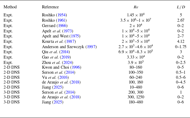


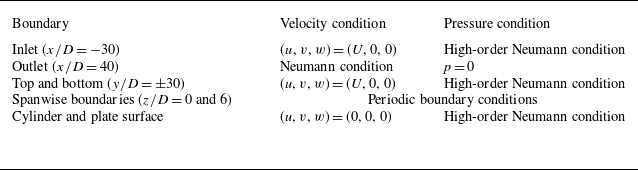


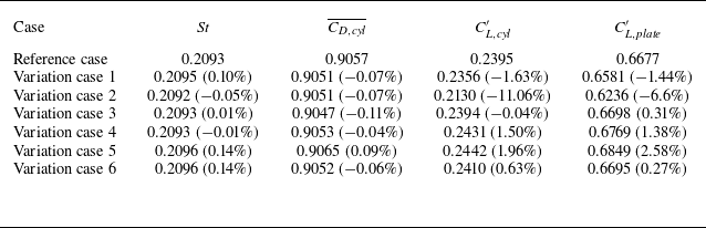


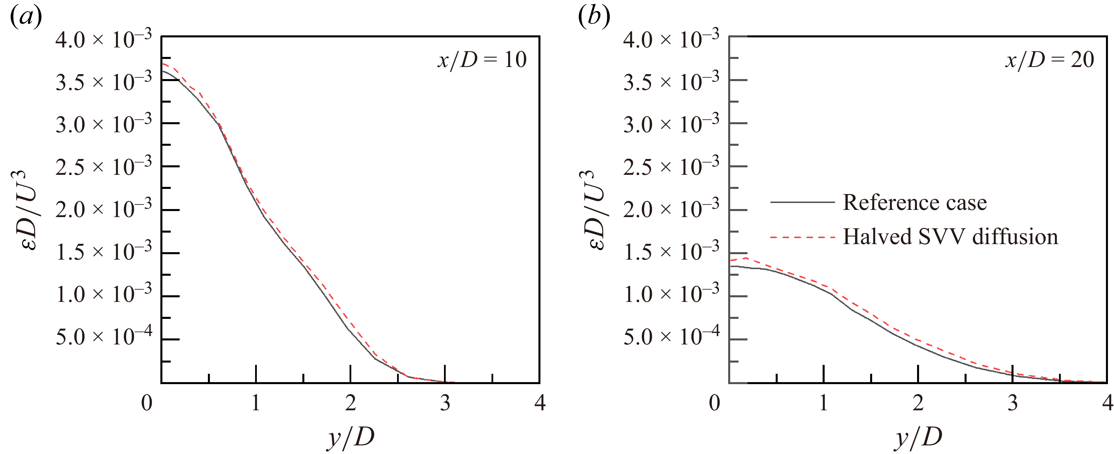


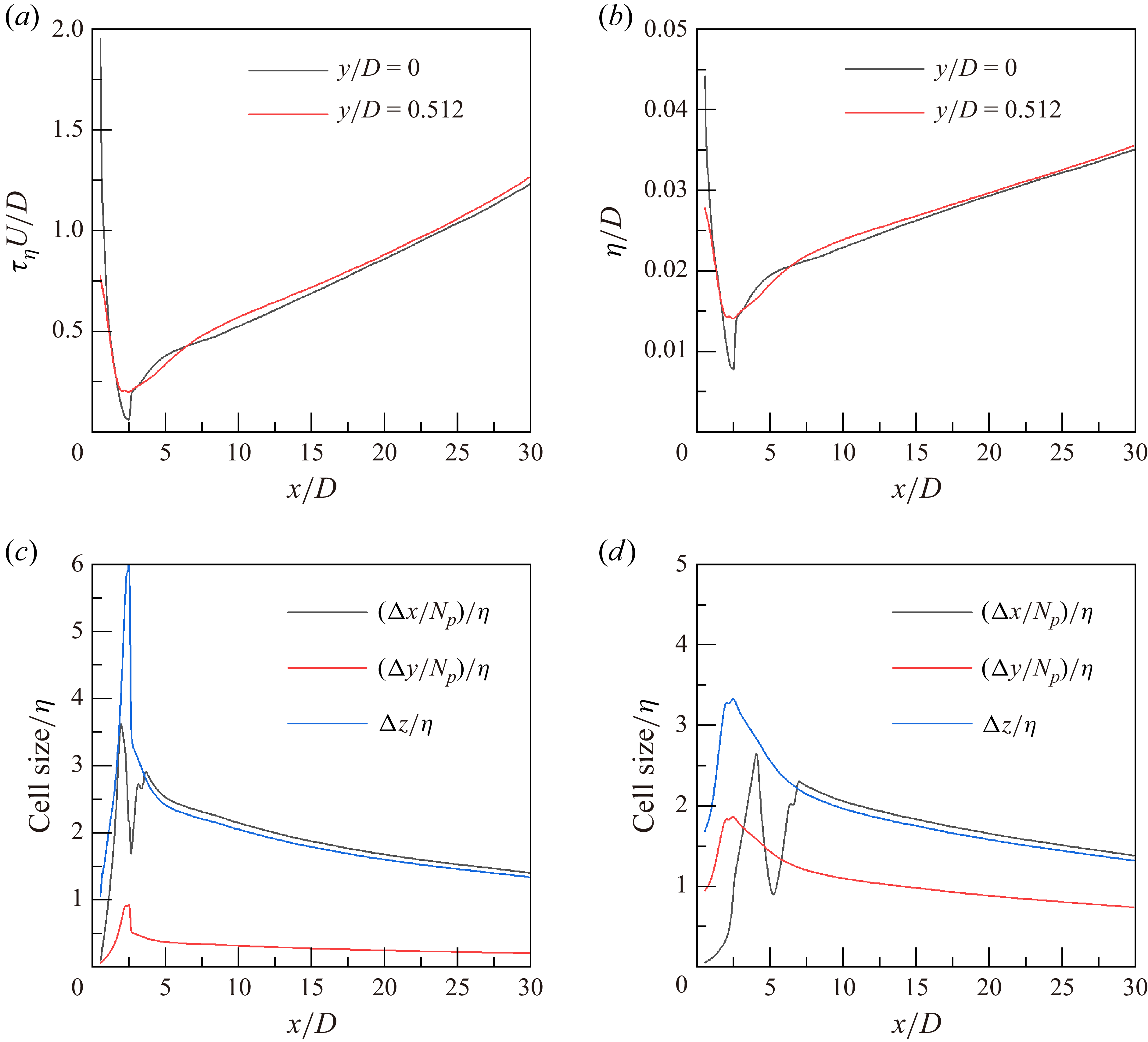


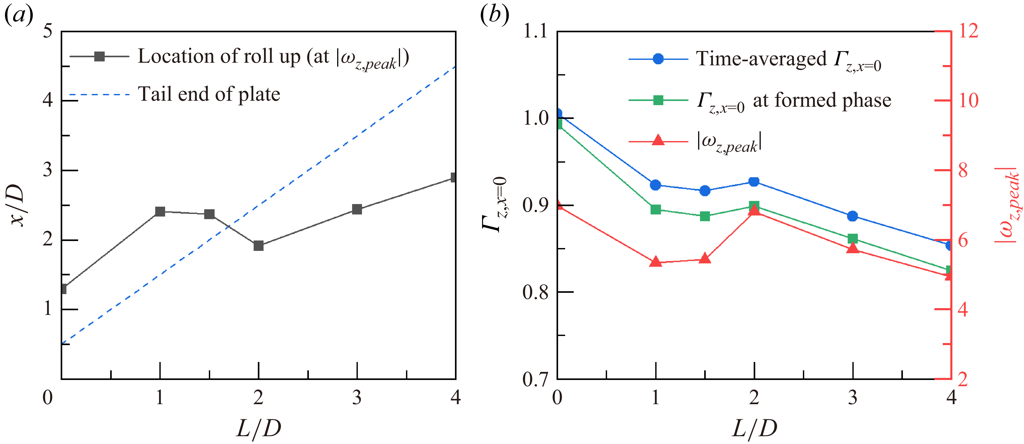


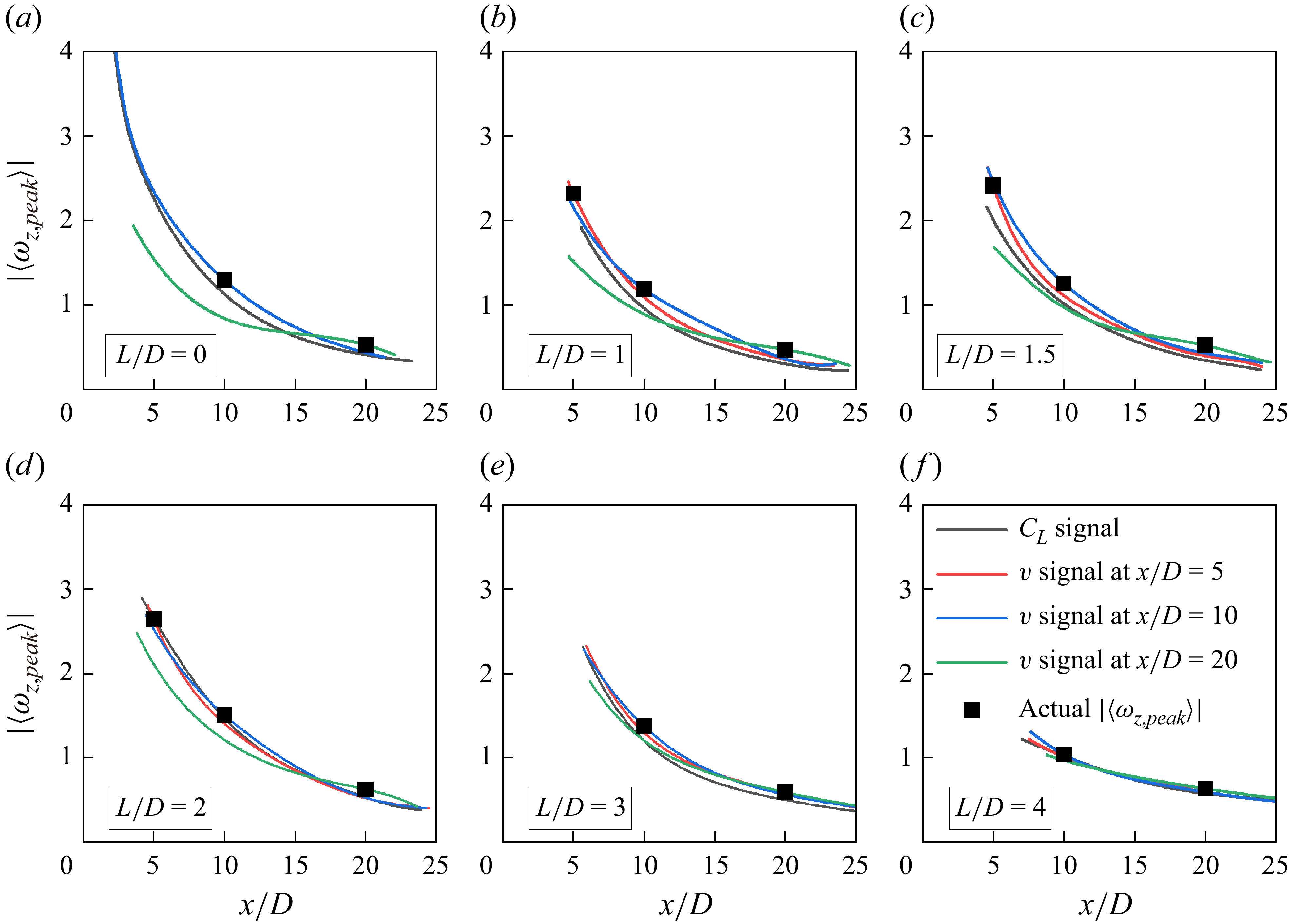


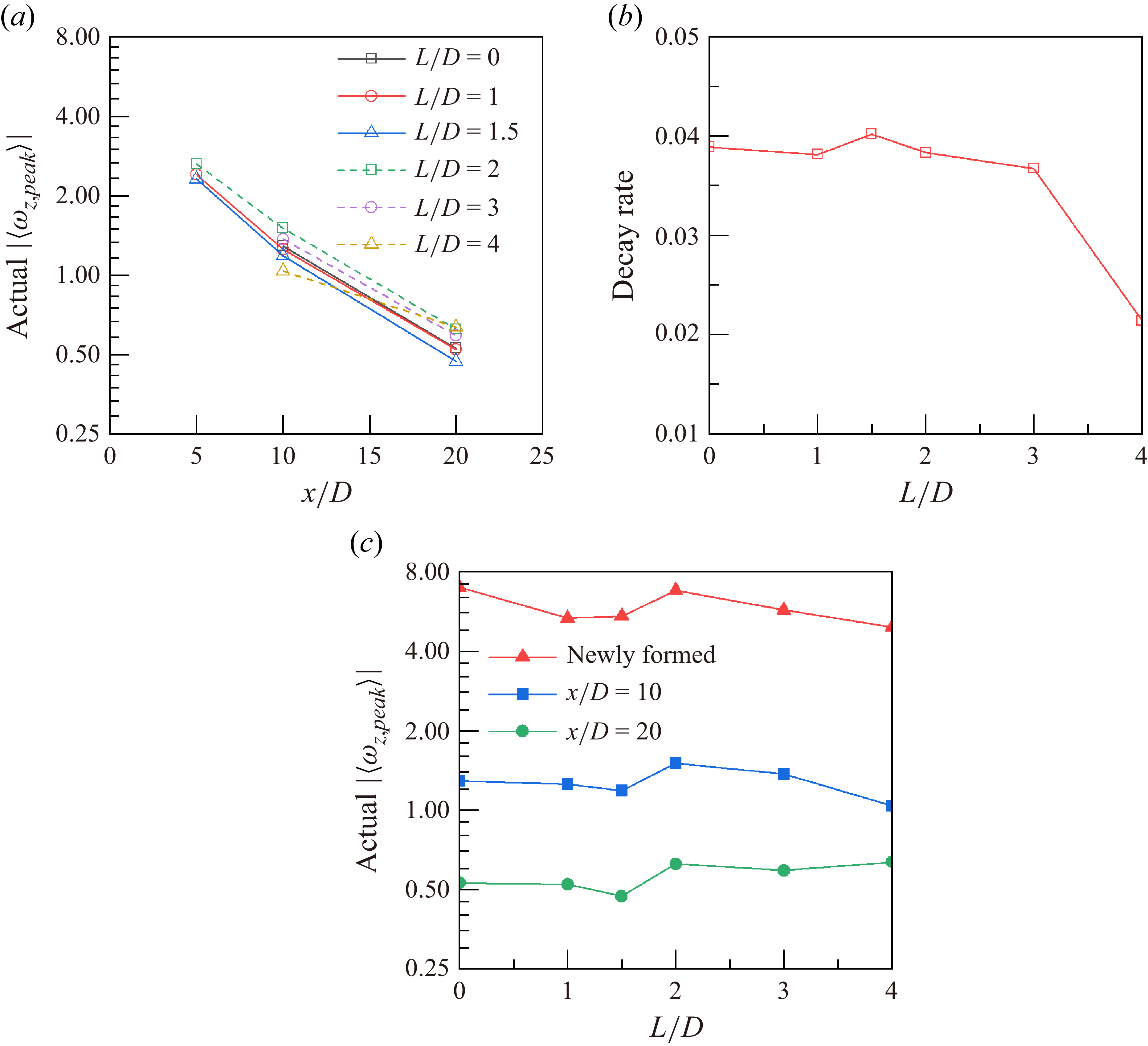


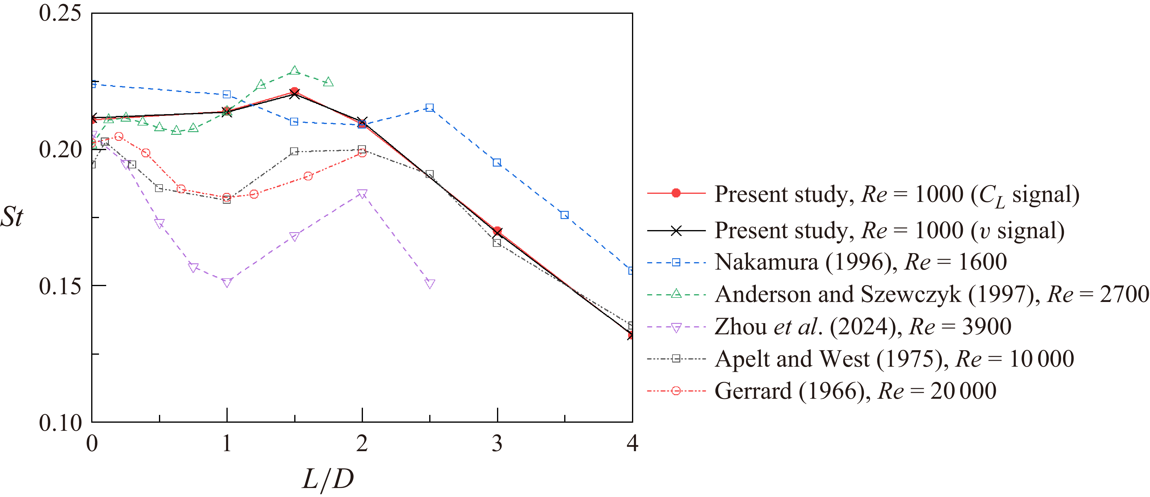


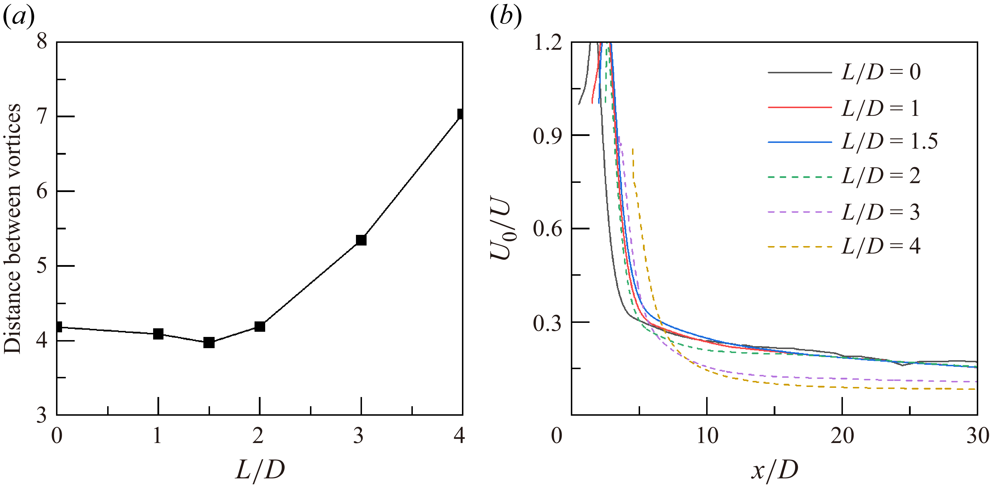

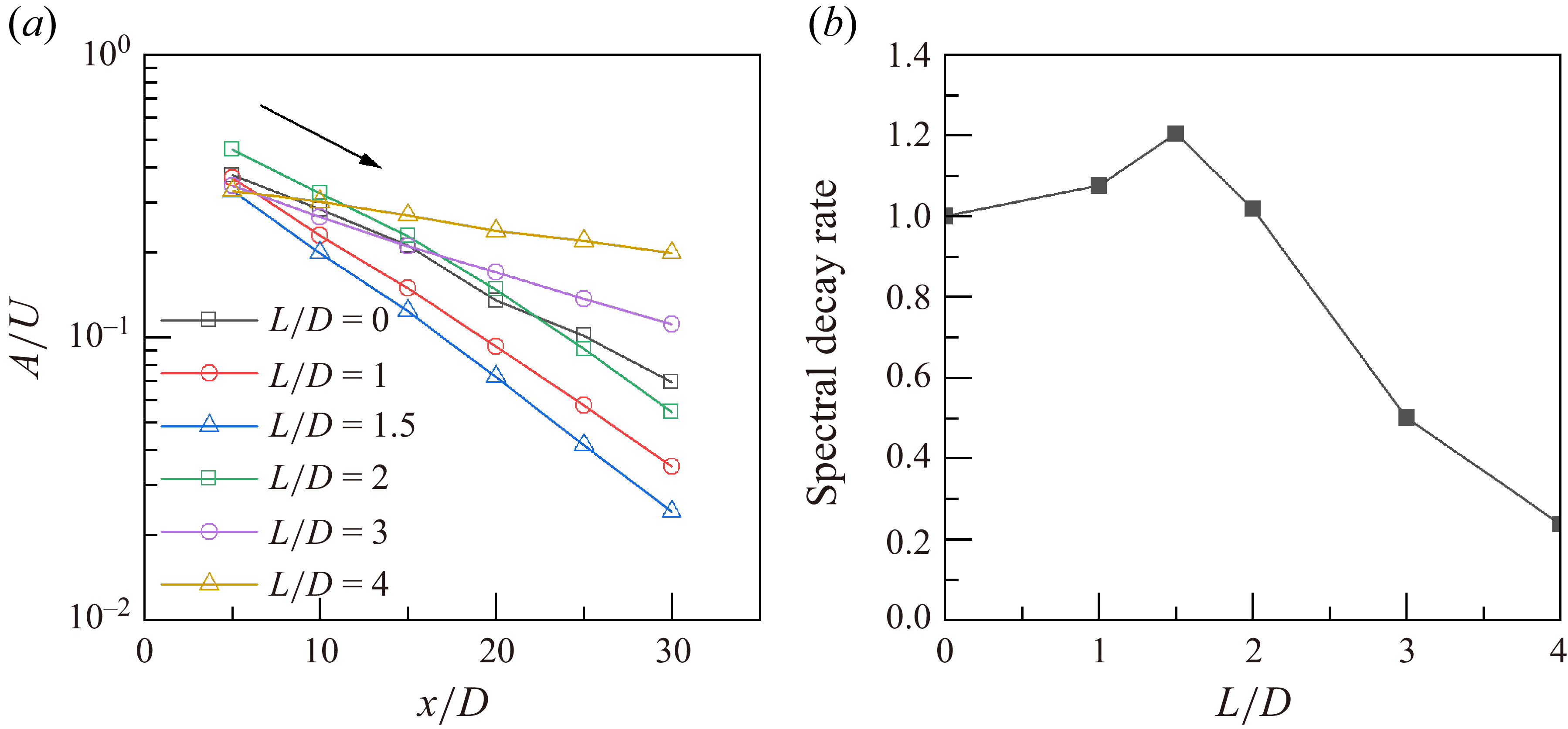


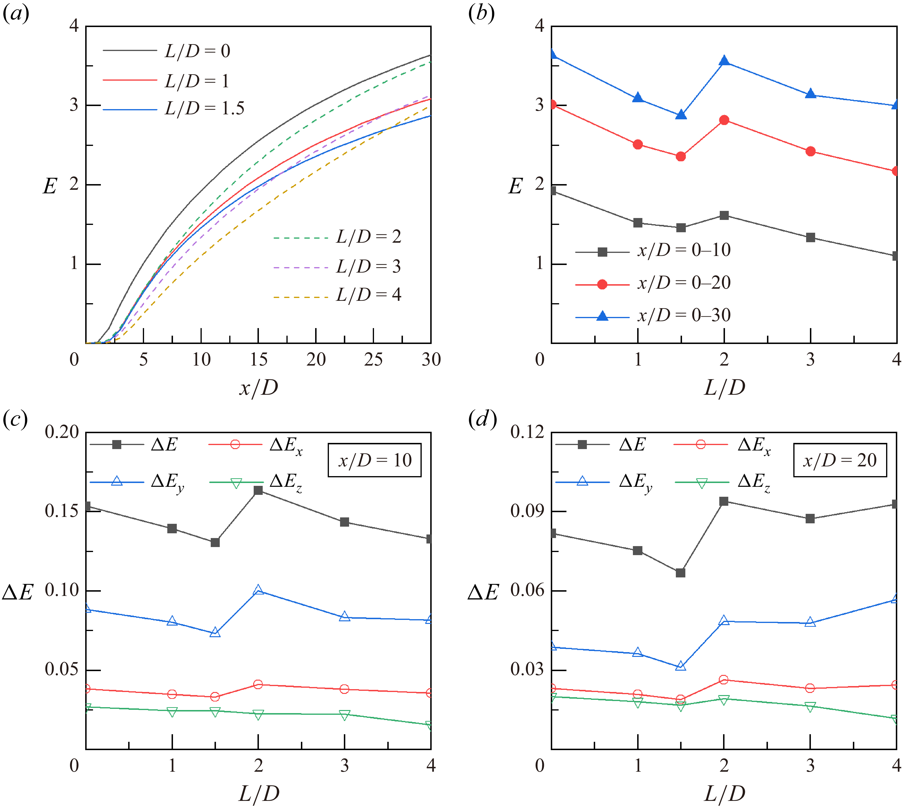


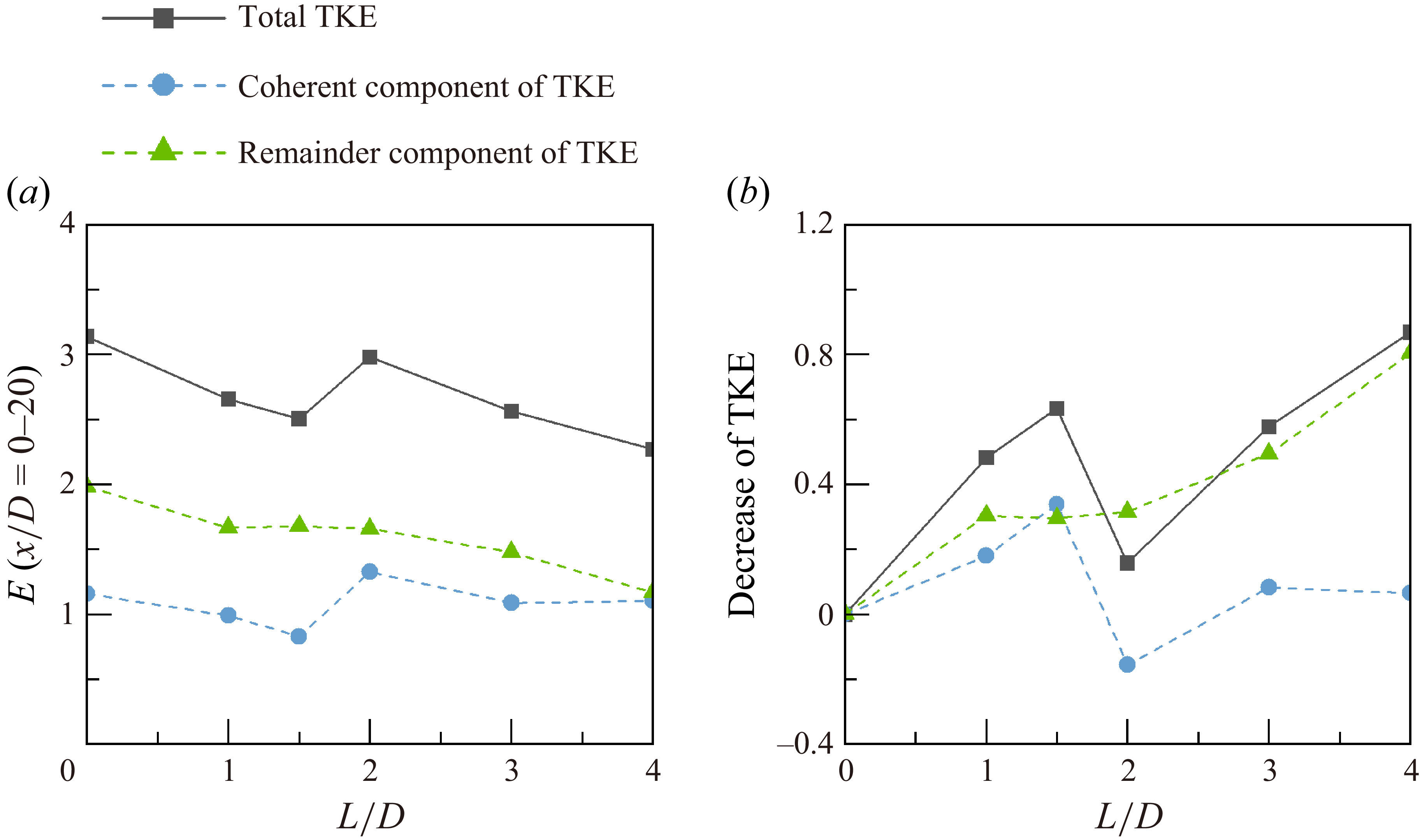


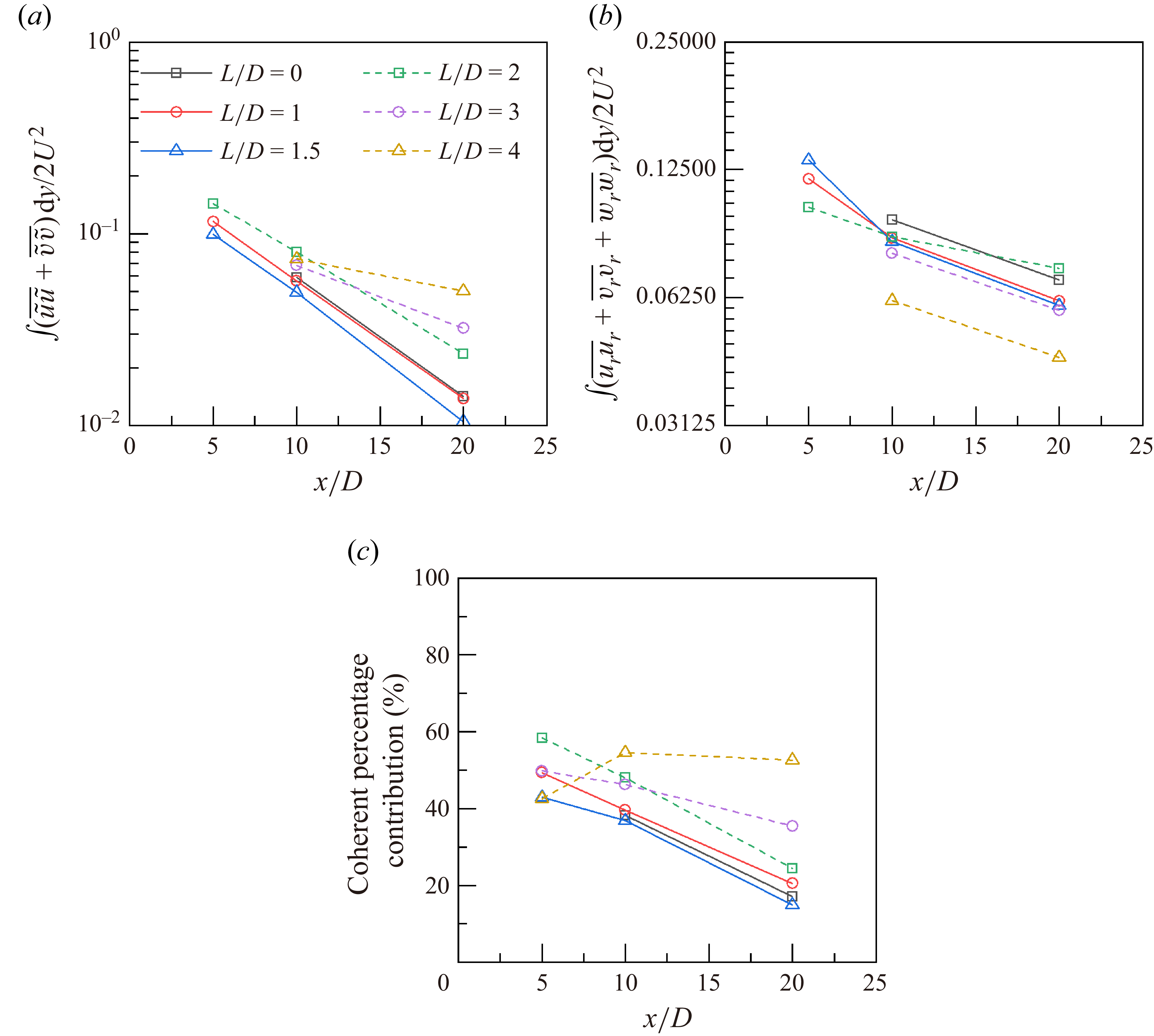


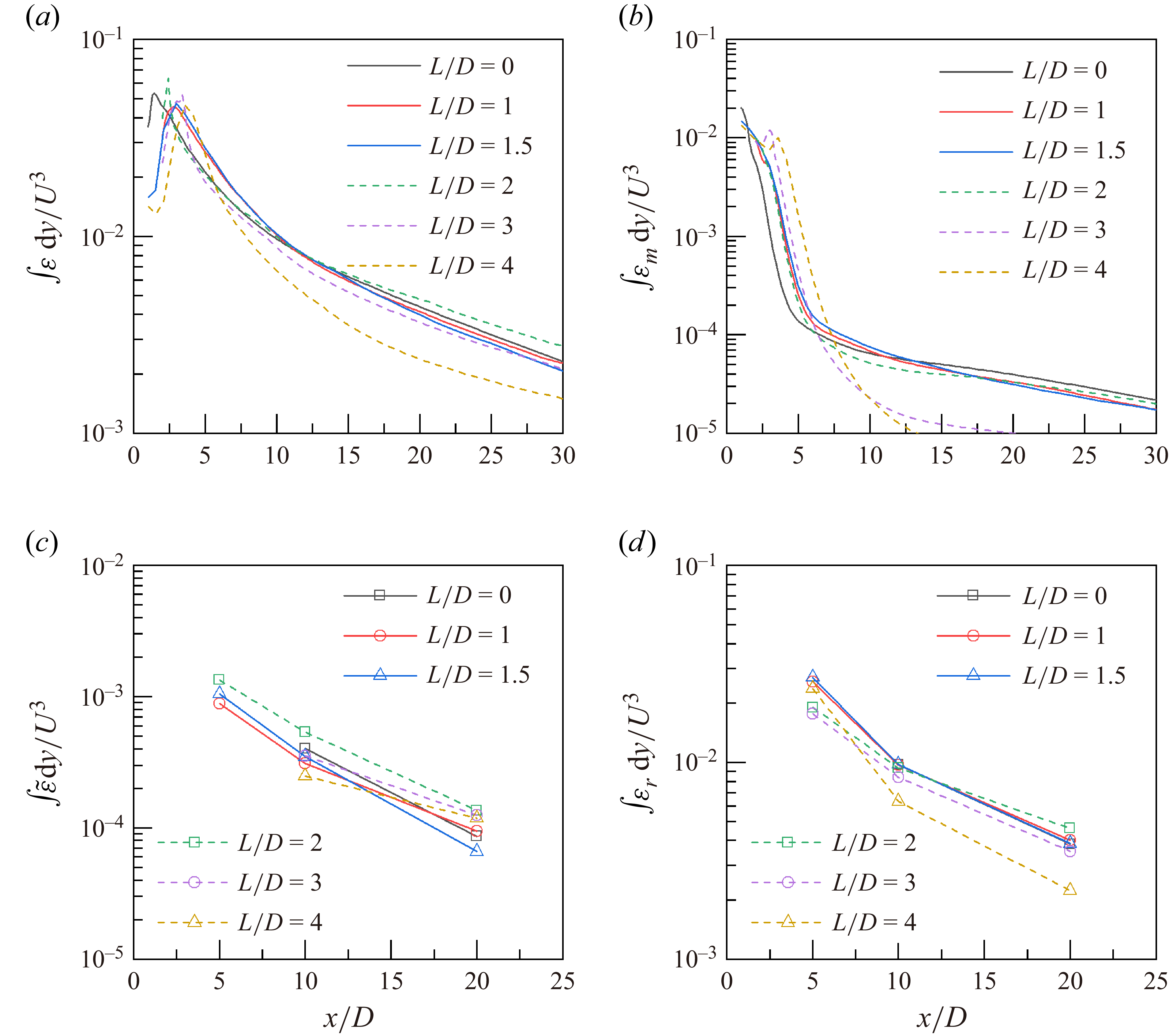


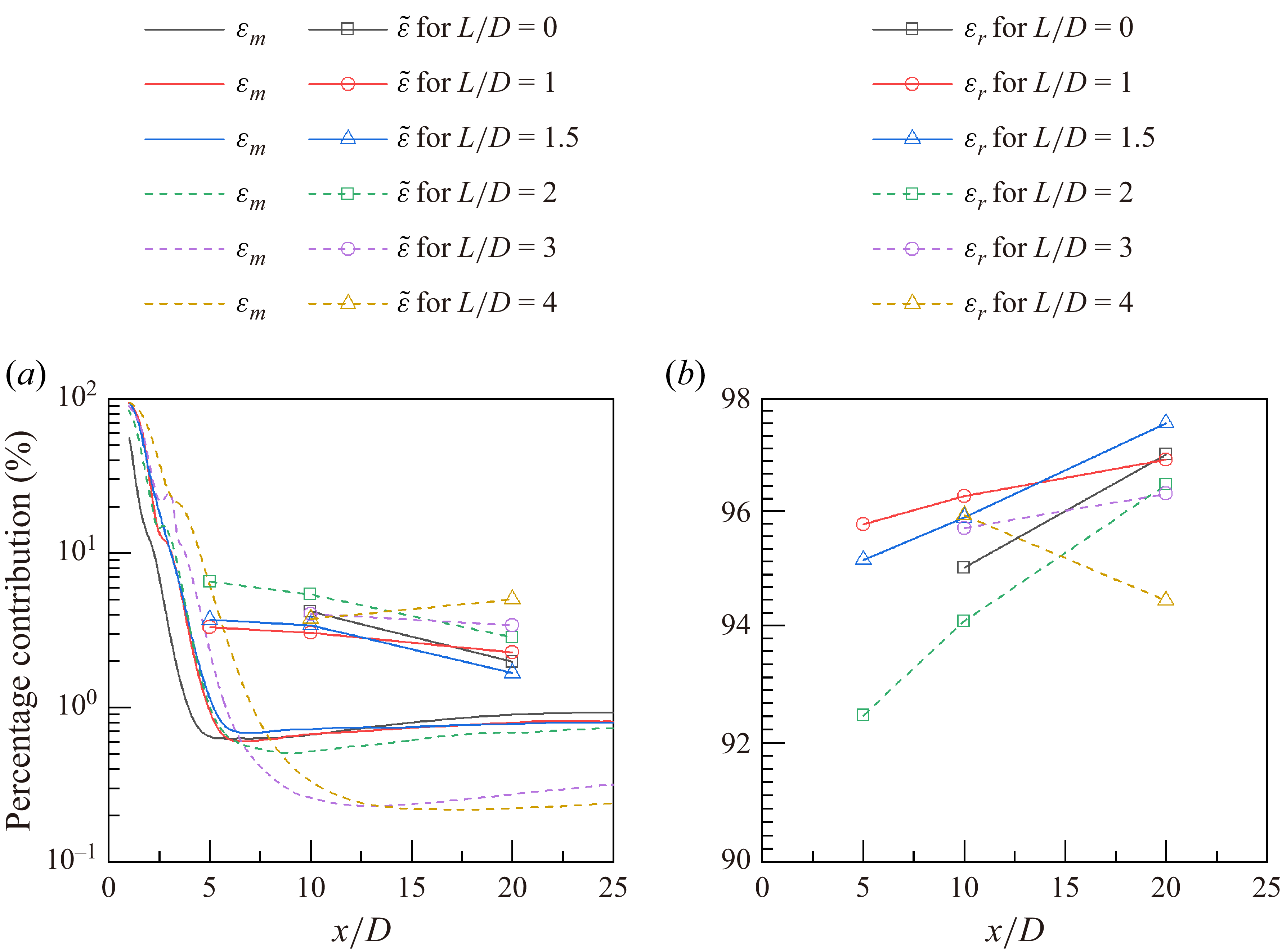


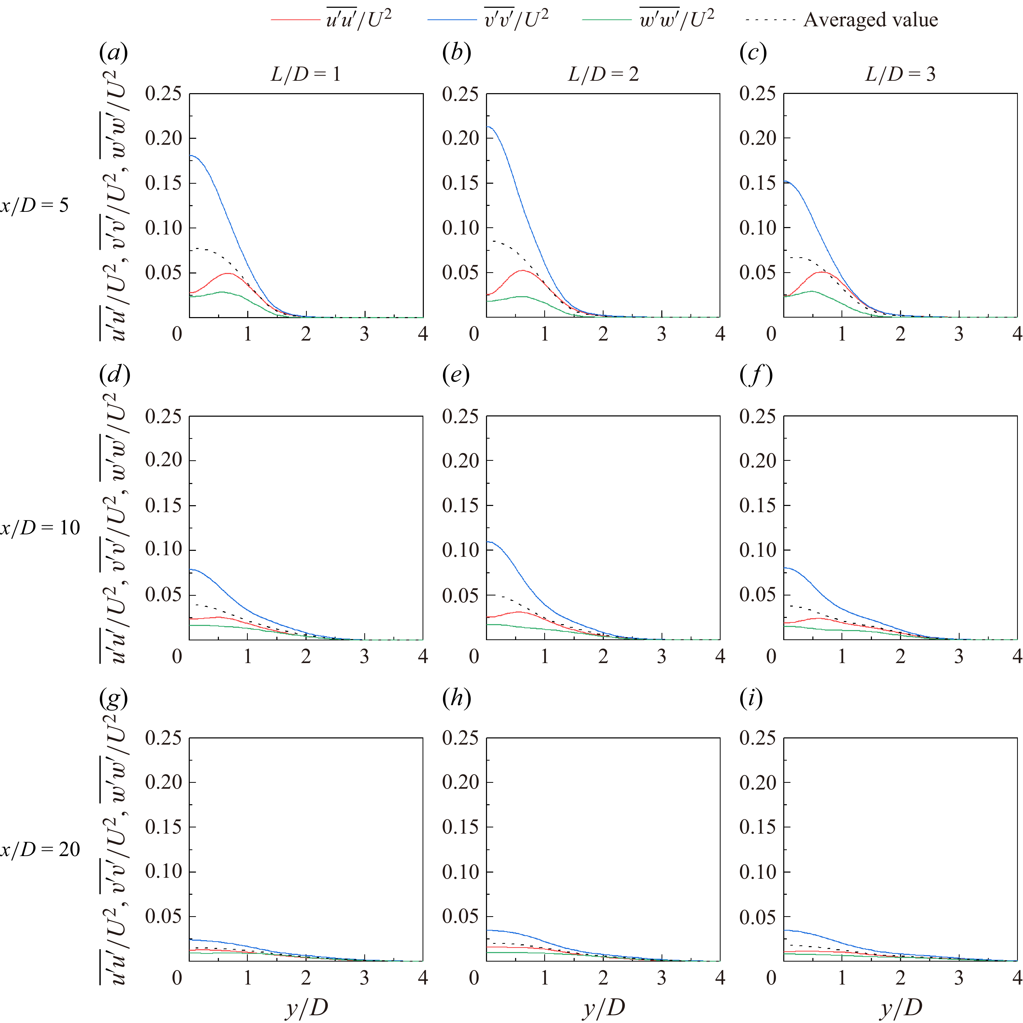


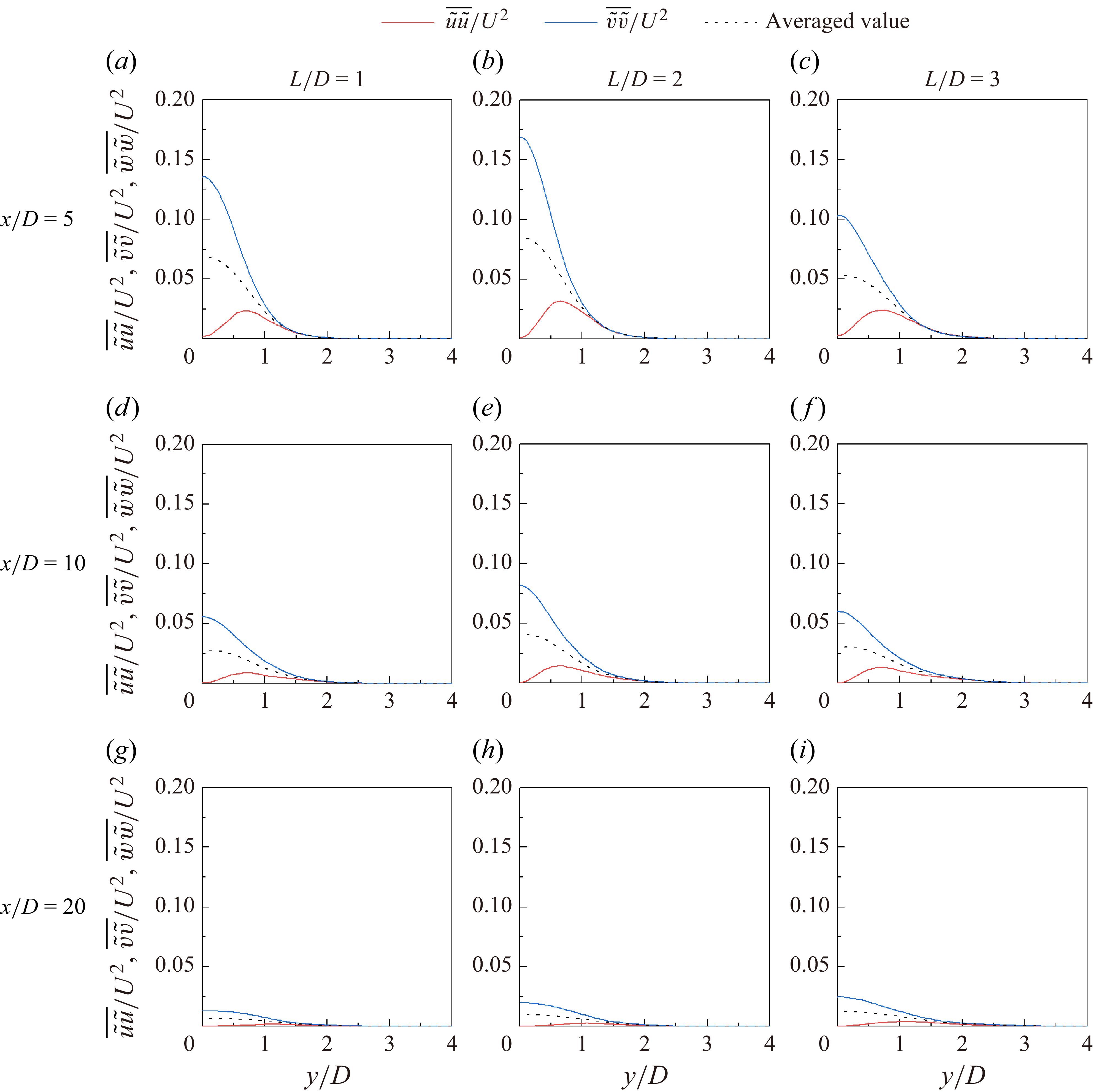


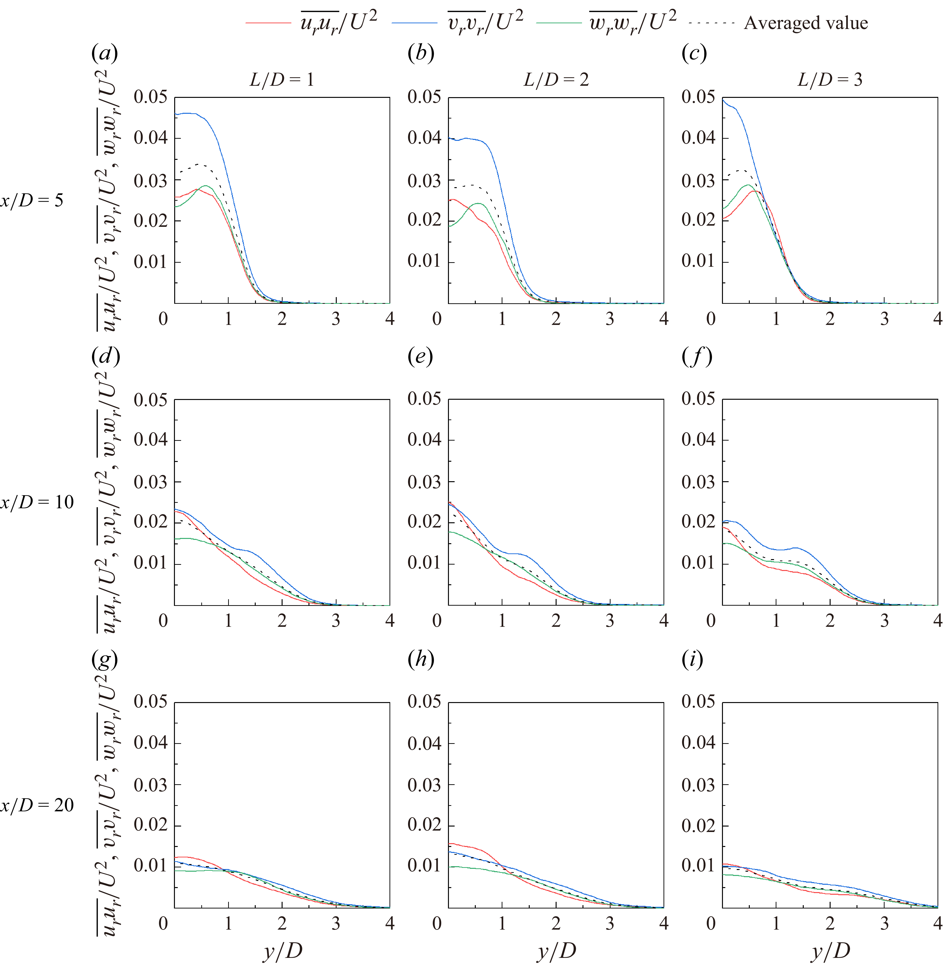


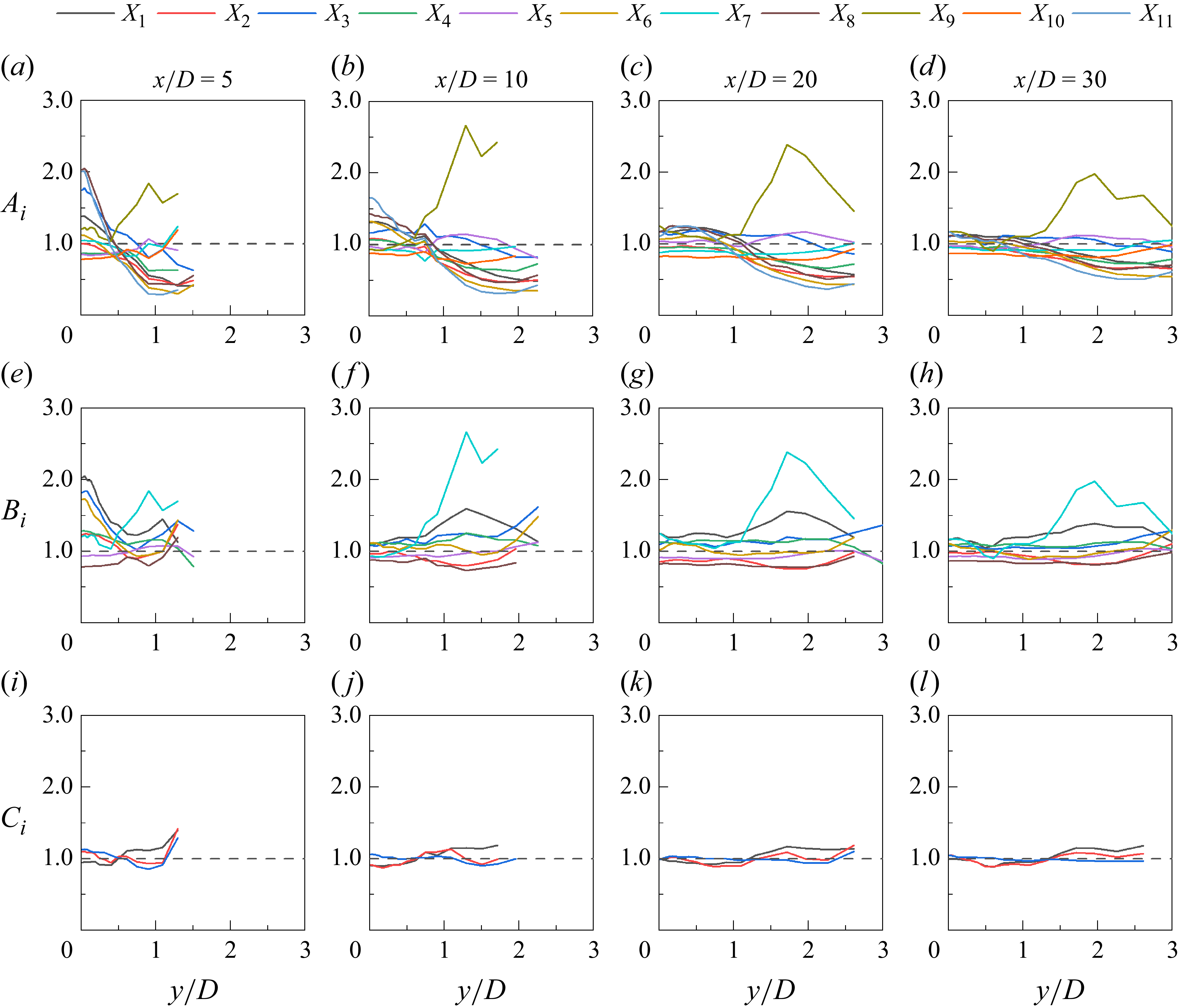

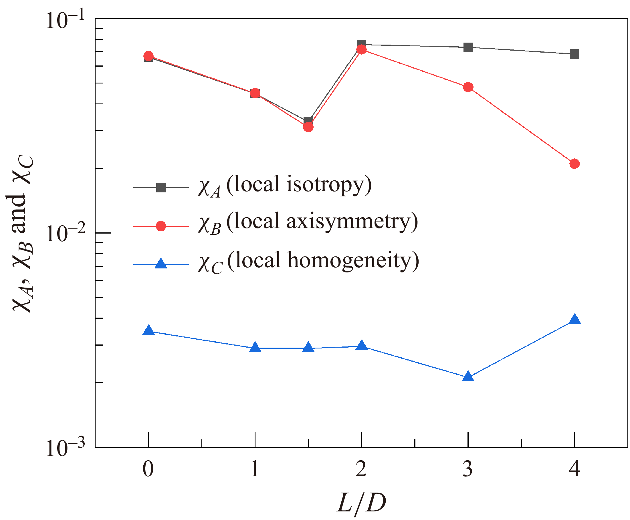


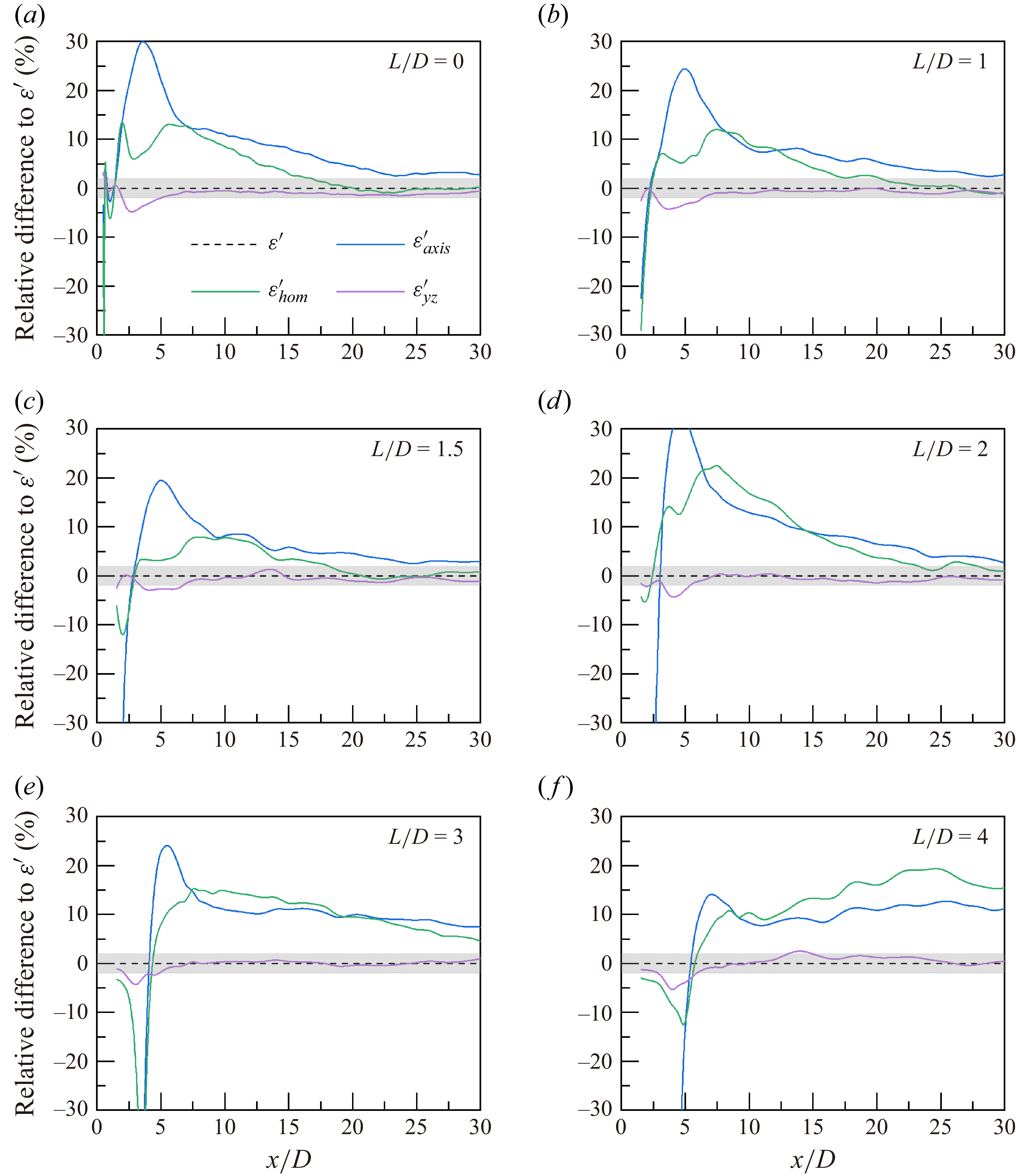


 Open access