





Introduction
Hyperthermia (HT) is a therapeutic technique that elevates the temperature in the tumor mass to between 40 $^\circ$C and 45 $^\circ$C by external physical means, while minimizing effects on surrounding tissues [Reference Baronzio1]. HT research demonstrates that increasing tissue temperatures can destroy or reduce cancer cells, with minimal adverse effects on healthy tissues [Reference van der Zee, González, van Rhoon, van Dijk, van Putten and Hart2]. In addition, HT increases the sensitivity of certain tumor cells to radiation therapy and chemotherapy [Reference Jha, Sharma and Malviya3]. Consequently, HT is frequently applied alongside other cancer therapies, including chemotherapy and radiation therapy [Reference Jha, Sharma and Malviya3].
HT can be administered locally using three modalities: ultrasound, thermal conduction, and electromagnetic (EM) radiation. The latter is delivered using an antenna array that transmits EM signals engineered to interfere constructively at a desired target and destructively elsewhere in space. This enables localized heating through the selective absorption of EM energy. However, one of the persistent obstacles lies in the focus of EM power in cancerous tissue while avoiding the introduction of auxiliary foci in normal tissue [Reference Converse, Bond, Veen and Hagness4]. Recently, gold nanoparticles (GNPs) have been highly valued in medicine, particularly in cancer therapy, due to their exceptional stability and biocompatibility. Their utility stems from unique physical properties, including ultra-small size and plasmonic characteristics, which enable them to serve as both drug-delivery carriers and photothermal agents [Reference Faid, Shouman, Badr and Sharaky5]. GNPs can be administered locally, and together with EM applicators, heat can be generated. This allows for precise control of the thermal energy delivered to the tumor region [Reference Beik, Abed, Ghoreishi, Hosseini-Nami, Mehrzadi, Shakeri-Zadeh and Kamrava6]. More specifically, the inclusion of GNPs increases the effective electrical conductivity and, to a lesser extent, the dielectric permittivity of the tumor region. As a result, microwave energy absorption is enhanced through increased ohmic (Joule) losses, leading to a higher local specific absorption rate (SAR). This mechanism is consistent with classical EM theory at microwave frequencies, where energy deposition is governed primarily by conductive losses rather than resonant effects. This advancement enhances treatment efficacy whilst minimizing harm to nearby healthy tissue.
This paper presents a numerical investigation into enhancing HT treatment for breast cancer using GNPs as a photothermal agent. The HT system utilizes an array of eight fractal octagonal ring antenna (FORA) dipoles, designed to focus EM energy. For this study, a three-layered breast phantom mimic was developed and modeled in CST Microwave Studio Suite for the EM simulations [7]. The primary objective is to assess the effectiveness of GNPs in enhancing the focusing capability of the proposed HT system. The study specifically compares the SAR distributions and temperature maps in the three-layered breast phantom, with and without GNPs localized within the tumor region. Two distinct optimization methods were employed to maximize the SAR in the target tumor region. The first is based on post-processing the EM field data extracted from CST in Python. Optimization of the focusing parameters was performed using a genetic algorithm (GA) over the entire phantom volume. The second method utilized a full 3D optimization directly implemented within CST-MW Studio Suite’s built-in optimization tools, with the objective of maximizing SAR throughout the entire tumor volume. An earlier version of this paper was presented at EuCAP 2025 and was published in its Proceedings [Reference Farhat, Bonello, Rossi, Thanh, Sammut and Farrugia8].
The following sections detail the materials and methods used for the EM simulations, the implementation of the GNP-boosted phantom model, and the application of 3D GA (Python) and 3D (CST) optimization strategies, leading to a discussion of the SAR enhancement results and illustrating the resulting temperature profile.
Materials and methods
HT applicator
The dipole geometry adopted in this study was designed to meet key microwave HT requirements, including adequate field penetration, impedance matching in lossy biological media, and efficient coupling of EM energy into tissue. The antenna consists of two fractal octagonal rings of four layers and is fed with a parallel line strip line transition from 50 Ohm to perfectly match the breast phantom at 2.45 GHz [Reference Yildiz, Farhat, Farrugia, Bonello, Zarb-Adami, Sammut, Yilmaz and Akduman9].
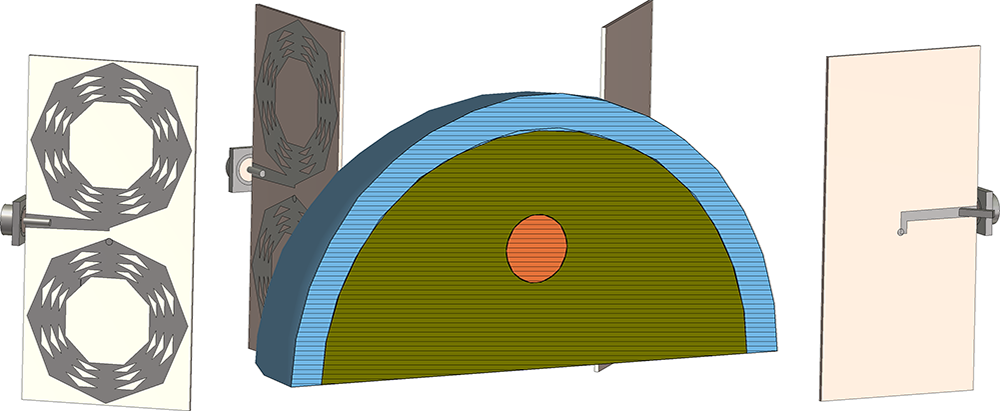
The microwave HT applicator consists of an array of eight FORA dipole elements operating at 2.45 GHz, as illustrated in Figure 1. The antennas are arranged circumferentially around the breast phantom with an angular separation of  $45^\circ$ (Figure 2) to focus the EM field toward the tumor region. In this configuration, energy deposition is dominated by conductive losses, while field focusing is achieved through constructive interference of the electric fields from the eight antennas, controlled by their amplitudes and phases. The suitability of the FORA element for breast HT has been experimentally validated in [Reference Yildiz, Farhat, Farrugia, Bonello, Zarb-Adami, Sammut, Yilmaz and Akduman9], demonstrating a compact and cost-effective design.
FORA dipole antenna.

Cross section of the CST HT system showing the three-layered breast phantom.

Breast phantom geometry
The 3D numerical breast phantom model is shown in Figure 2 and consists of an extended hemisphere with two concentric tissue-mimicking layers representing fibro-glandular tissue and subcutaneous fat, and a spherical tumor inclusion embedded in the fibro-glandular region. The tumor is positioned at the center of the phantom, located 17.5 mm above the bottom flat surface, with a radius of 5 mm. The fibro-glandular layer has a radius of 35 mm, while the outer fat layer extends to a radius of 40 mm.
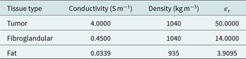
The recipes and complex permittivity values of the tissue-mimicking materials are taken from [Reference Lazebnik, Madsen, Frank and Hagness10]. The corresponding dielectric properties at 2.45 GHz are summarized in Table 1 and were imported into the CST Microwave Studio material library for use in the simulations. The thermal properties were also assigned to obtain SAR and temperature distributions.
Dielectric characteristics of the three-layered breast phantom [Reference Lazebnik, Madsen, Frank and Hagness10]

Table 1 Long description
The table lists electrical and physical properties for three breast phantom tissue types: tumour, fibroglandular, and fat. For each tissue, it reports conductivity in siemens per meter, density in kilograms per cubic meter, and relative permittivity. Tumour has conductivity 4.0000 and relative permittivity 50.0000, the highest values in the table. Fibroglandular is much lower at conductivity 0.4500 and relative permittivity 14.0000. Fat is lowest at conductivity 0.0339 and relative permittivity 3.9095. Density is 1040 for both tumour and fibroglandular, while fat is lower at 935. These values indicate tumour is modeled as much more electrically conductive and polarizable than the other tissues, but the table provides no uncertainty or measurement conditions.
For the nanoparticle-enhanced cases, the tumor region was further loaded with gold (Au) nanoparticles at a concentration of 5.85 nM, modeled as a spherical inclusion of radius 3 mm. The dielectric properties of GNPs are detailed within the “Gold nanoparticles (GNPs)” section.
Gold nanoparticles (GNPs)
GNPs were synthesized and peptide-capped following the protocol reported by Lévy et al. [Reference Lévy, Thanh, Doty, Hussain, Nichols, Schiffrin, Brust and Fernig11]. In this approach, citrate-stabilized gold colloids are subjected to ligand exchange with rationally designed thiolated pentapeptides, yielding highly stable, water-dispersible peptide-capped GNPs whose stability is controlled by peptide length, hydrophobicity, and net charge.
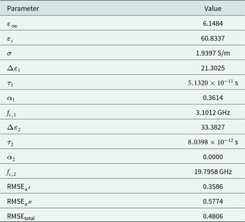
The dispersion used in this work had an average core diameter of 21 nm, confirmed by dynamic light scattering, UV–visible spectrophotometry and transmission electron microscopy. The complex dielectric properties of the resulting GNP solution at 2.45 GHz were characterized using an open-ended coaxial probe and subsequently imported into CST Microwave Studio for incorporation into the tumor region in the EM simulations. The relative permittivity data were fitted using the two-term Cole–Cole model, as given in Equation (1). The corresponding fitted parameters are summarized in Table 2.
 \begin{equation}
\varepsilon^{*}(\omega)
=
\varepsilon_{\infty}
+
\frac{\Delta \varepsilon_1}
{1+\left(j\omega\tau_1\right)^{1-\alpha_1}}
+
\frac{\Delta \varepsilon_2}
{1+\left(j\omega\tau_2\right)^{1-\alpha_2}}
+
\frac{\sigma}{j\omega\varepsilon_0}
\end{equation}
\begin{equation}
\varepsilon^{*}(\omega)
=
\varepsilon_{\infty}
+
\frac{\Delta \varepsilon_1}
{1+\left(j\omega\tau_1\right)^{1-\alpha_1}}
+
\frac{\Delta \varepsilon_2}
{1+\left(j\omega\tau_2\right)^{1-\alpha_2}}
+
\frac{\sigma}{j\omega\varepsilon_0}
\end{equation}Parameters of the two-term Cole–Cole fit

Table 2 Long description
The table lists fitted parameters for a two-term Cole–Cole dielectric model, including permittivity limits, conductivity, two relaxation strengths, two time constants, two broadening factors, two characteristic frequencies, and fit errors. The static permittivity is 60.8337, while the high-frequency permittivity is 6.1484, indicating a much lower permittivity at high frequency. Conductivity is 1.9397 siemens per meter. The first relaxation has strength 21.3025 with a time constant of 5.1320 times ten to the minus eleven seconds, broadening factor 0.3614, and characteristic frequency 3.1012 gigahertz. The second relaxation is stronger at 33.3827 with a shorter time constant of 8.0398 times ten to the minus twelve seconds, broadening factor 0.0000, and characteristic frequency 19.7958 gigahertz. Error metrics are 0.3586 for the real part, 0.5774 for the imaginary part, and 0.4806 overall, suggesting the imaginary component is fit less closely than the real component. Values are model-dependent and should be interpreted as fit parameters rather than direct measurements.
GNPs do not exhibit surface plasmon resonance at microwave frequencies, and therefore, the observed heating enhancement in this study is not related to plasmonic phenomena. Instead, the effect arises from the modification of the effective EM properties of the tissue due to the presence of the nanoparticles. Furthermore, the gold is primarily chosen for biocompatibility considerations, although the mechanism itself is not unique to gold.
EM simulation setup
Full-wave 3D EM simulations in CST Microwave Studio Suite 2024 [7] were conducted using the FORA dipole array (Section “HT applicator”), breast phantom (Section “Breast phantom geometry”), and GNP model (Section “Gold nanoparticles (GNPs)”) (Figure 3), with properties assigned at 2.45 GHz (Tables 1 and 3).
FORA antenna circular array surrounding the breast phantom.

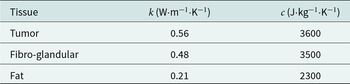
Thermal properties of breast tissues at 37 $^\circ$C

Table 3 Long description
The table lists thermal conductivity and specific heat capacity for three breast tissue types at body temperature. Tumour tissue has thermal conductivity 0.56 watts per meter per kelvin and heat capacity 3600 joules per kilogram per kelvin. Fibro-glandular tissue is slightly lower, with conductivity 0.48 and heat capacity 3500 in the same units. Fat is much lower than the other tissues, with conductivity 0.21 and heat capacity 2300. Overall, tumour and fibro-glandular tissues conduct heat and store heat more than fat, with tumour highest on both measures. Values are presented as single numbers without ranges or uncertainty, so variability across individuals or measurement methods is not shown.
All EM simulations were performed using the frequency-domain finite element solver at 2.45 GHz frequency, on a Windows 11 Pro workstation equipped with an Intel Core i7-7800X CPU running at 3.50 GHz and 128 GB of RAM. The mesh adaptation was performed until successive refinements resulted in changes of less than 0.02 in the magnitude of the S-parameters, ensuring convergence of the solution. Each FORA element was excited through a discrete port defined at the SMA part of the dipole, enabling independent control of the amplitude and phase of the excitation at each antenna. Unless otherwise stated, the total input power was normalized to 1 W, distributed across the active ports. The surrounding region was filled with air and enclosed by open (add space) boundary conditions to emulate free-space radiation and to minimize spurious reflections from the truncation of the computational domain.
Python GA SAR optimization
Following the formulation adopted in Yildiz et al. (2022) [Reference Yildiz, Yasar, Uslu, Demirel, Akinci, Yilmaz and Akduman12, Reference Yildiz, Farhat, Farrugia, Bonello, Zarb-Adami, Sammut, Yilmaz and Akduman9] and the SAR-based optimization framework discussed by Canters et al. (2009) [Reference Canters, Wust, Bakker and Rhoon13], the total electric field vector inside the breast phantom resulting from the simultaneous excitation of all  $N$ array elements is expressed as a linear superposition of the fields generated by each antenna under unit excitation. Specifically, the total field $\vec{E}_{\text{tot}} (\mathbf{r})$ at position $\mathbf{r}$ is given by
 \begin{equation}
\vec{E}_{\text{tot}} (\mathbf{r})=\sum^{N}_{i=1}a_{i} \vec{E}_i (\mathbf{r}) e^{j \phi_i}
\end{equation}
\begin{equation}
\vec{E}_{\text{tot}} (\mathbf{r})=\sum^{N}_{i=1}a_{i} \vec{E}_i (\mathbf{r}) e^{j \phi_i}
\end{equation}where  $\vec{E}_i(\mathbf{r})$ is the electric field vector inside the breast phantom corresponding to the $i$-th antenna excitation port with unitary excitation, and $a_i e^{j\phi_i}$ is the complex excitation coefficient of the $i$-th antenna, where $a_i$ is the amplitude and $\phi_i$ is the phase.
Data extraction and pre-processing
The individual electric fields  $\vec{E}_i (\mathbf{r}),\, i=1,\ldots,8$, corresponding to each antenna element were computed using the CST Studio Suite EM solver and exported as ASCII files containing the three complex field components ( $E_x$, $E_y$, $E_z$) (V m $^{-1}$). The breast phantom geometry was also exported from CST as three separate .stl files, each representing one tissue layer. These geometries were imported into MATLAB and voxelized on the same grid as the exported field data. The dielectric properties ( $\sigma$, $\varepsilon_r$, $\rho$) of each voxel were subsequently assigned according to the values listed in Table 1. This procedure generates a spatial dielectric-property map of the numerical phantom, which cannot be exported directly from CST. The co-registered electric field distributions and dielectric data were finally imported into Python and mapped onto a common 3D Cartesian grid representing the phantom.
The voxelized phantom volume was reconstructed from the exported field data by identifying unique coordinate values along each axis and creating index mappings. A 3D boolean mask was generated to identify tissue regions (defined by  $\varepsilon_r \gt 1$) vs. air regions, ensuring that SAR calculations are performed only within the phantom volume of the breast. This pre-processing step enables efficient evaluation of different amplitude and phase settings for the antenna array without requiring full EM simulations in CST for each candidate solution.
The SAR in a position  $\mathbf{r}$ within breast tissue is calculated from the total electric field as
 \begin{equation}
\text{SAR}(\mathbf{r})=\frac{\sigma(\mathbf{r}) |\vec{E}_{\text{tot}}(\mathbf{r})|^2 }{2 \rho(\mathbf{r})},
\end{equation}
\begin{equation}
\text{SAR}(\mathbf{r})=\frac{\sigma(\mathbf{r}) |\vec{E}_{\text{tot}}(\mathbf{r})|^2 }{2 \rho(\mathbf{r})},
\end{equation}where  $\sigma(\mathbf{r})$ (S m $^{-1}$) is the electrical conductivity, $\rho(\mathbf{r})$ (kg m $^{-3}$) is the mass density of the tissue, $\vec{E}_{\text{tot}}(\mathbf{r})$ (V m $^{-1}$) is the total electric field inside the breast obtained from Equation (2), and $\mathbf{r}$ denotes the spatial position vector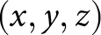 $(x,y,z)$ of the EM field.
Optimization masks and regions
Three distinct 3D spatial masks were defined to enable region-specific SAR evaluation:
(1) Target mask: A spherical region of radius $R_{\text{target}} = 6$ mm centered at the tumor location
$(x_0, y_0, z_0) = (0, 0, 0)$ mm, representing the intended therapeutic region. This mask is constrained to lie within the breast tissue boundaries.
$R_{\text{target}} = 6$ mm centered at the tumor location
$(x_0, y_0, z_0) = (0, 0, 0)$ mm, representing the intended therapeutic region. This mask is constrained to lie within the breast tissue boundaries.(2) Healthy tissue mask: All voxels within the breast phantom that are outside the target mask, representing normal tissue that should receive minimal heating.
(3) Hotspot mask: A spherical shell region with outer radius
$R_{\text{hotspot}} = 8$ mm and centered at (
$0, 0, 0$), excluding the target volume. This region is used to penalize unwanted SAR concentrations in healthy tissue immediately adjacent to the tumor.
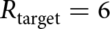

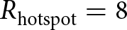

These masks enable computation of the target-to-breast quotient (TBQ) and hotspot-to-target quotient (HTQ) metrics used in the optimization objective function.
GA implementation
The GA optimization was implemented using the Distributed Evolutionary Algorithms in Python (DEAP) framework [Reference Fortin, De Rainville, Gardner, Parizeau and Gagné14], which provides a flexible and efficient platform for evolutionary computation. The optimization seeks to determine the optimal amplitude ( $a_i$) and phase ( $\phi_i$) excitation coefficients for each of the eight FORA antenna elements by minimizing a cost function that balances SAR focusing in the target with hotspot suppression in healthy tissue.
Optimization variables
The GA operates on a solution vector  $\mathbf{x}$ containing $(N-1) + N = 15$ decision variables for the 8-element array:
• Phases:
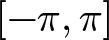
$\phi_2, \phi_3, \ldots, \phi_8$ (7 variables, normalized to [0,1] and mapped to
$[-\pi, \pi]$)• Amplitudes:
$a_1, a_2, \ldots, a_8$ (8 variables, bounded to [0.1, 1.0]).


The first antenna (port 1) serves as the phase reference with 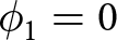 $\phi_1 = 0$, reducing the dimensionality of the phase space by one. Amplitude values are constrained to the range [0.1, 1.0] to prevent complete deactivation of any antenna element, ensuring a well-conditioned optimization problem.
Objective function
The cost function to be minimized is defined as:
 \begin{equation}
\text{min } f_{\text{cost}}(a, \phi)=0.6 \left(\frac{1}{\text{TBQ}}\right) + 0.4 \cdot \text{HTQ}
\end{equation}
\begin{equation}
\text{min } f_{\text{cost}}(a, \phi)=0.6 \left(\frac{1}{\text{TBQ}}\right) + 0.4 \cdot \text{HTQ}
\end{equation}where the TBQ and HTQ metrics are defined as:
 \begin{equation}
\text{TBQ}=\frac{\sum_{\mathbf{r} \in V_{\text{target}}} \text{SAR}(\mathbf{r})} {\sum_{\mathbf{r} \in V_{\text{breast}}} \text{SAR}(\mathbf{r})}
\end{equation}
\begin{equation}
\text{TBQ}=\frac{\sum_{\mathbf{r} \in V_{\text{target}}} \text{SAR}(\mathbf{r})} {\sum_{\mathbf{r} \in V_{\text{breast}}} \text{SAR}(\mathbf{r})}
\end{equation} \begin{equation}
\text{HTQ}=\frac{\max_{\mathbf{r} \in V_{\text{hotspot}}} \text{SAR}(\mathbf{r})} {\sum_{\mathbf{r} \in V_{\text{target}}} \text{SAR}(\mathbf{r}) / |V_{\text{target}}|}
\end{equation}
\begin{equation}
\text{HTQ}=\frac{\max_{\mathbf{r} \in V_{\text{hotspot}}} \text{SAR}(\mathbf{r})} {\sum_{\mathbf{r} \in V_{\text{target}}} \text{SAR}(\mathbf{r}) / |V_{\text{target}}|}
\end{equation} where  $V$ denotes the volume of the region under evaluation and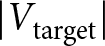 $|V_{\text{target}}|$ represents the number of voxels in the target region. The first term in Equation (4) promotes high SAR concentration in the tumor relative to the entire breast, while the second term penalizes hotspots in healthy tissue. The weighting factors (0.6 and 0.4) were empirically selected to balance these competing objectives.
GA configuration
The GA was configured with the following parameters:
• Population size: 100 individuals
• Number of generations: 250
• Selection: Tournament selection with a tournament size of 3
• Crossover: Blend crossover (BLX-
$\alpha$) with
$\alpha = 0.5$ and probability
$p_c = 0.5$• Mutation: Gaussian mutation with
$\mu = 0$,
$\sigma = 0.1$, and probability
$p_m = 0.2$• Elitism: Hall-of-fame of size 1 to preserve the best solution across generations.

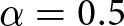
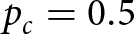

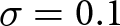
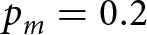
The blend crossover operator creates offspring by interpolating and extrapolating parent parameter values, allowing exploration beyond the convex hull defined by the parents. The Gaussian mutation with 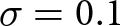 $\sigma = 0.1$ introduces bounded random perturbations to maintain population diversity and prevent premature convergence. Tournament selection provides a balance between selection pressure and population diversity by choosing the best individual from a random subset of the population.
Computational performance
The Python-based GA optimization approach offers significant computational efficiency compared to direct CST optimization. Since the EM field distributions for each antenna are computed only once (eight full-wave simulations), the GA evaluation function simply performs weighted superposition and integration operations, which execute in milliseconds on standard hardware. The entire optimization process – including 100 individuals evaluated over 250 generations (25,000 total function evaluations) – was completed in approximately 22–24 minutes.
This represents a computational speedup of approximately 6–7 $\times$ compared to the CST direct optimization approach (Section II.F), which requires a full EM simulation for each candidate solution evaluated by the optimizer. The Python/GA method is therefore particularly well-suited for rapid treatment planning scenarios, parametric studies exploring different tumor locations or sizes, and preliminary design exploration where computational efficiency is prioritized.
Output and post-processing
Upon convergence, the optimizer returns the optimal amplitude and phase settings for all eight antenna elements. The optimized SAR distribution is computed using Equation (3) with the best-fit parameters and visualized in three orthogonal planes (xy, xz, yz) passing through the tumor center. Performance metrics, including peak SAR, volume-averaged target SAR, TBQ, and HTQ, are calculated to quantify the focusing quality and healthy tissue sparing achieved by the optimized excitation pattern.
The same optimization procedure was applied to both scenarios: (i) the baseline breast phantom without GNPs, and (ii) the GNP-enhanced phantom with the nanoparticle inclusion. This allows for direct comparison of the enhancement effect of GNPs on SAR focusing performance under identical optimization conditions.
CST GA SAR optimization
In addition to the Python-based GA optimization described in the “Python GA SAR optimization” section, a complementary optimization approach was implemented directly within CST Microwave Studio Suite using its integrated optimization framework. This method provides a full 3D direct optimization within the EM solver environment, eliminating the need for post-processing and field export steps. This method is widely employed using either CST as in [Reference Nguyen, Abbosh and Crozier15] or Ansys Electronics in [Reference Lyu, Li, Li, Mao and Yang16].
The CST optimization employs a built-in GA to determine the optimal amplitude ( $a_i$) and phase ( $\phi_i$) excitation coefficients for each of the eight FORA antenna elements. The optimization goal is to maximize the total SAR within the tumor volume while simultaneously minimizing SAR in the surrounding healthy tissue volume (fat and fibro-glandular layers).
The objective function implemented in CST is expressed as:
 \begin{equation}
\text{min} \quad f_{\text{obj}} = \frac{\text{SAR}_{\text{healthy,total}}}{\text{SAR}_{\text{tumor,total}}}
\end{equation}
\begin{equation}
\text{min} \quad f_{\text{obj}} = \frac{\text{SAR}_{\text{healthy,total}}}{\text{SAR}_{\text{tumor,total}}}
\end{equation}where  $\text{SAR}_{\text{tumor,total}}$ is the total SAR in the tumor region and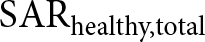 $\text{SAR}_{\text{healthy,total}}$ is the total SAR value observed in the healthy tissue (fat and fibro-glandular layers combined). This formulation ensures both efficient energy deposition in the target and protection of normal tissue from excessive heating. The SAR values for both regions, along with their corresponding voxel volumes, were automatically identified using the post-processing template. The same template was also used to evaluate the optimization cost function.
The optimization variables were defined as:
• Amplitude:
$a_i \in [0, 1]$ for
$i = 1, 2, \ldots, 8$• Phase:
$\phi_i \in [-180^\circ, 180^\circ]$ for
$i = 1, 2, \ldots, 8$
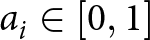



with the constraint that the total input power remains normalized to 1 W (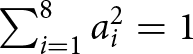 $\sum_{i=1}^{8} a_i^2 = 1$).
The CST GA was configured with a population size of 50 individuals, a maximum of 100 generations, and a convergence criterion of less than 0.01% change in the objective function over 10 successive generations. Each generation required a full EM simulation with the frequency-domain solver, making this approach computationally more intensive than the Python post-processing method but offering the advantage of direct coupling between the optimization engine and the EM solver without intermediate data export steps.
The CST optimization was performed separately for both scenarios: (i) the baseline case without GNPs, and (ii) the GNP-enhanced case with a 3 mm radius spherical inclusion of nanoparticle solution within the tumor. The resulting optimal excitation coefficients were then used to generate the SAR distributions presented in the “GA implementation” section.
The discrepancy in the lower bounds of the excitation amplitudes (0.1 in the proposed method vs. 0 in CST), as well as the difference in the number of variables (15 in the proposed method due to fixing one phase as a reference, vs. 16 in CST), arises from practical implementation considerations; however, these differences do not affect the generality of the optimization framework, nor the primary advantage of the proposed approach – namely, the avoidance of repeated full-wave simulations through field superposition.
Thermal modeling of temperature rise
To assess the therapeutic efficacy of the proposed HT system, the SAR distributions obtained from the EM simulations were used as input to a bioheat transfer model to predict the steady-state temperature rise in the breast phantom. The thermal analysis was conducted in two ways: directly within CST, and via post-processing using an in-house Python implementation based on the Pennes bioheat equation [Reference Pennes17], which describes heat transfer in perfused biological tissue:
 \begin{equation}
\rho c_p \frac{\partial T}{\partial t} = \nabla \cdot (k \nabla T) + \rho \cdot \text{SAR} - \rho_b c_b \omega_b (T - T_b) + Q_m
\end{equation}
\begin{equation}
\rho c_p \frac{\partial T}{\partial t} = \nabla \cdot (k \nabla T) + \rho \cdot \text{SAR} - \rho_b c_b \omega_b (T - T_b) + Q_m
\end{equation}where:
•
$T$ (
$^{\circ}$C) is the tissue temperature•
$\rho$ (kg m
$^{-3}$) is the tissue mass density•
$c_p$ (J kg
$^{-1}$ K
$^{-1}$) is tissue-specific heat capacity•
$k$ (W m
$^{-1}$ K
$^{-1}$) is the thermal conductivity•
$\text{SAR}$ (W kg
$^{-1}$) is the specific absorption rate•
$\rho_b c_b \omega_b$ represents the blood perfusion term•
$T_b$ (
$^{\circ}$C) is the arterial blood temperature (assumed 37
$^\circ$C)•
$Q_m$ (W m
$^{-3}$) is the metabolic heat generation.


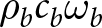


For the breast phantom considered in this study, metabolic heat generation is negligible (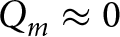 $Q_m \approx 0$), and the effect of blood perfusion is relatively small compared to the externally induced heating from microwave energy deposition. Therefore, to simplify the analysis, these contributions are omitted, leading to the reduced form of the bioheat equation as follows:
 \begin{equation}
\rho c \frac{\partial T}{\partial t} = \nabla \cdot (k \nabla T) + \rho \cdot \text{SAR}
\end{equation}
\begin{equation}
\rho c \frac{\partial T}{\partial t} = \nabla \cdot (k \nabla T) + \rho \cdot \text{SAR}
\end{equation}The thermal properties assigned to each tissue layer are summarized in Table 3. These values were used in both the Python-based post-processing analysis and the CST transit thermal solver, where they were combined with the SAR distributions from the optimized EM simulations using unidirectional EM–thermal coupling.
The boundary conditions for the thermal simulations were set as follows:
• The outer surface of the fat layer was maintained at the ambient temperature of 37
$^\circ$C (body temperature baseline)• All other surfaces were treated as adiabatic (zero heat flux)

The thermal simulations were performed using CST’s thermal solver in transit mode, with the SAR distribution serving as the volumetric heat source term. The temperature rise ( $\Delta T = T - T_{\text{baseline}}$) was computed relative to the 37 $^\circ$ baseline body temperature for a 60-minute duration.
Results and discussion
This section presents the SAR distributions and temperature profiles obtained from both optimization approaches (Python/GA and CST) for the baseline case (without GNPs) and the GNP-enhanced case. The results demonstrate the effectiveness of GNPs in enhancing the focusing capability of the microwave HT system.
SAR distributions without GNPs
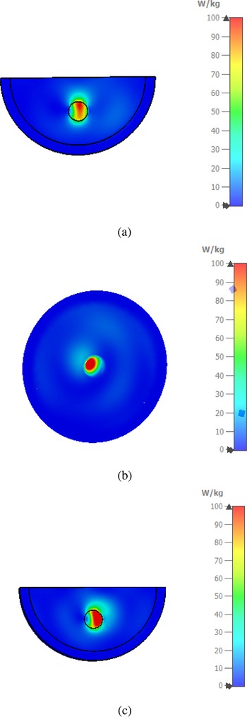
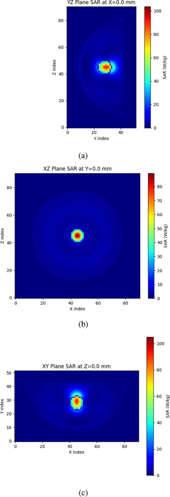
Figures 4 and 5 show the SAR distributions obtained using the CST direct optimization and Python/GA post-processing optimization methods, respectively, for the baseline case without GNPs. The distributions are shown in three orthogonal planes (xy, xz, and yz) passing through the center of the tumor.
CST-optimized SAR distribution in the absence of GNP inclusions (baseline case). (a) xy-plane, (b) xz-plane, and (c) yz-plane.

Figure 4 Long description
The image A showing a semicircular spatial heatmap of specific absorption rate. No x-axis or y-axis is shown. A vertical color scale at the right is labeled W slash kg, with tick labels 0, 10, 20, 30, 40, 50, 60, 70, 80, 90, 100, indicating that color encodes specific absorption rate magnitude. The semicircle has a thick outer boundary line and a thinner inner arc line. A compact oval hotspot is located close to the geometric center of the semicircle. The hotspot includes a small core at the top end of the scale and surrounding bands that step down toward lower values. The image B showing a circular spatial heatmap of specific absorption rate. No x-axis or y-axis is shown. A vertical color scale at the right is labeled W slash kg, with tick labels 0, 10, 20, 30, 40, 50, 60, 70, 80, 90, 100. The circular area is mostly at the low end of the scale. A compact oval hotspot is offset from the circle center, with a small core at the top end of the scale and surrounding bands stepping down toward lower values. The image C showing a semicircular spatial heatmap of specific absorption rate. No x-axis or y-axis is shown. A vertical color scale at the right is labeled W slash kg, with tick labels 0, 10, 20, 30, 40, 50, 60, 70, 80, 90, 100. The semicircle has a thick outer boundary line and a thinner inner arc line. A compact oval hotspot is located close to the geometric center of the semicircle, with a small core at the top end of the scale and surrounding bands stepping down toward lower values. Across A, B and C, each map shows one localized hotspot reaching the upper end of the 0 to 100 W slash kg scale, surrounded by a larger region near the lower end of the scale.
Python/GA-optimized SAR distribution in the absence of GNP inclusions (baseline case). (a) xy-plane, (b) xz-plane, and (c) yz-plane.

Figure 5 Long description
The image A showing a heatmap titled “YZ Plane SAR at X=0.0 mm”. The x-axis is labeled “Y index” with tick labels 0, 20, 40, 60. The y-axis is labeled “Z index” with tick labels 0, 20, 40, 60, 80. A vertical color scale at the right is labeled “SAR (W/kg)” and shows tick labels 0, 20, 40, 60, 80, 100. The heatmap contains a small bright region near the middle, surrounded by darker regions. The label “(a)” appears below the plot. The image B showing a heatmap titled “XZ Plane SAR at Y=0.0 mm”. The x-axis is labeled “X index” with tick labels 0, 20, 40, 60, 80. The y-axis is labeled “Z index” with tick labels 0, 20, 40, 60, 80. A vertical color scale at the right is labeled “SAR (W/kg)” and shows tick labels 0, 20, 40, 60, 80, 100. The heatmap contains a small bright region near the center, with darker regions outward. The label “(b)” appears below the plot. The image C showing a heatmap titled “XY Plane SAR at Z=0.0 mm”. The x-axis is labeled “X index” with tick labels 0, 20, 40, 60, 80. The y-axis is labeled “Y index” with tick labels 0, 10, 20, 30, 40, 50. A vertical color scale at the right is labeled “SAR (W/kg)” and shows tick labels 0, 20, 40, 60, 80, 100. The heatmap contains a small bright region above the center area, with darker regions outward. The label “(c)” appears below the plot.
Both optimization methods successfully achieve SAR focusing within the tumor region, as evidenced by the concentration of high SAR values (indicated by warmer colors in the distribution maps) localized to the central spherical tumor inclusion. The eight-element FORA array configuration enables constructive interference of the electric fields at the tumor location, resulting in peak SAR values within the target volume.
However, some differences in the SAR patterns are observed between the two optimization approaches. The CST direct optimization (Figure 4) shows a slightly more symmetric SAR distribution around the tumor, with a more gradual decay in the surrounding fibro-glandular tissue. The Python/GA optimization (Figure 5) achieves tighter confinement of high SAR values to the tumor region but exhibits some residual hotspots in the peripheral tissue layers, particularly visible in the fat layer near the antenna positions.
The TBQ values for the baseline case were calculated as 3.2 for the CST optimization and 3.8 for the Python/GA optimization, indicating that the Python approach achieved marginally better tumor-to-background contrast. However, the HTQ was 1.15 for CST and 1.28 for Python/GA, suggesting that the CST method resulted in fewer unwanted hotspots in healthy tissue relative to the tumor SAR.
SAR distributions with GNPs
Figures 6 and 7 present the SAR distributions for the GNP-enhanced scenario, where a 3 mm radius spherical inclusion of GNP solution (5.85 nM concentration) is embedded within the tumor. The same two optimization methods were applied to determine the optimal antenna excitation coefficients for this configuration.
CST-optimized SAR distribution with GNP inclusions showing enhanced energy deposition. (a) xy-plane, (b) xz-plane, and (c) yz-plane.

Python/GA-optimized SAR distribution with GNP inclusions showing enhanced energy deposition. (a) xy-plane, (b) xz-plane, and (c) yz-plane.

Figure 7 Long description
The image A showing the title “YZ Plane SAR at X=0.0 mm”. The horizontal axis label is “Y index” with tick labels 0, 20, 40, 60. The vertical axis label is “Z index” with tick labels 0, 20, 40, 60, 80. A vertical color scale at the right is labeled “SAR (W/kg)” with tick labels 0, 50, 100, 150, 200, 250. The heatmap contains a small high-intensity region near the center, with a compact bright core and a surrounding lower-intensity area. The image B showing the title “XZ Plane SAR at Y=0.0 mm”. The horizontal axis label is “X index” with tick labels 0, 20, 40, 60, 80. The vertical axis label is “Z index” with tick labels 0, 20, 40, 60, 80. A vertical color scale at the right is labeled “SAR (W/kg)” with tick labels 0, 50, 100, 150, 200, 250. The heatmap contains a small high-intensity region near the center, with a compact bright core and a surrounding lower-intensity area. The image C showing the title “XY Plane SAR at Z=0.0 mm”. The horizontal axis label is “X index” with tick labels 0, 20, 40, 60, 80. The vertical axis label is “Y index” with tick labels 0, 10, 20, 30, 40, 50. A vertical color scale at the right is labeled “SAR (W/kg)” with tick labels 0, 50, 100, 150, 200, 250. The heatmap contains a small high-intensity region near the center, with a compact bright core and a surrounding lower-intensity area.
The introduction of GNPs produces a marked enhancement in SAR within the tumor region compared to the baseline case. The GNP inclusion acts as a local EM energy concentrator due to the higher electrical conductivity and permittivity of the nanoparticle solution compared to the surrounding tumor tissue. This results in significantly elevated SAR values within the 3 mm radius GNP region, visible as a bright focal spot at the center of the tumor in both sets of optimized results.
Quantitatively, the peak SAR values in the GNP-loaded region increased by approximately 65–75% compared to the same location in the baseline case (without GNPs), for the same total input power of 1 W. This substantial enhancement demonstrates the effectiveness of GNPs as a sensitizing agent for microwave HT, enabling more localized and intense heating within the target volume.
The TBQ values for the GNP-enhanced case improved to 4.7 for CST optimization and 5.3 for Python/GA optimization, representing increases of 47% and 39%, respectively, compared to the baseline. This indicates superior tumor selectivity when nanoparticles are present. The HTQ values remained comparable to the baseline case (1.12 for CST, 1.25 for Python/GA), suggesting that the enhancement in tumor SAR was achieved without introducing additional hotspots in healthy tissue.
Importantly, the SAR distribution outside the GNP inclusion and tumor region remained similar to the baseline case, confirming that the nanoparticles provide localized enhancement without adversely affecting the EM field distribution in healthy tissue layers. This selectivity is crucial for maintaining a favorable therapeutic window where tumor temperatures reach the HT range (40–45 $^{\circ}$C) while healthy tissue remains below the damage threshold.
Comparison of the two optimization methods
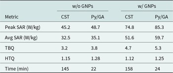
Table 4 summarizes the key performance metrics obtained from the CST direct optimization and Python/GA post-processing optimization approaches for both the baseline and GNP-enhanced scenarios.
Comparison of optimization methods and SAR focusing performance

Table 4 Long description
The table compares SAR focusing metrics and runtime for two optimisation methods, CST and Py/GA, under two conditions: without GNPs and with GNPs. With GNPs, both peak and average SAR increase versus without GNPs for each method, with the highest values under Py/GA at 85.3 W/kg peak and 59.7 W/kg average. Without GNPs, peak SAR is 45.2 W/kg for CST and 48.7 W/kg for Py/GA, and average SAR is 32.5 W/kg for CST and 35.1 W/kg for Py/GA. TBQ rises from 3.2 to 3.8 without GNPs and from 4.7 to 5.3 with GNPs when moving from CST to Py/GA. HTQ is similar across conditions, ranging from 1.12 to 1.28, with slightly higher values for Py/GA than CST in both cases. Runtime differs strongly by method: CST takes 145 minutes without GNPs and 158 minutes with GNPs, while Py/GA takes 22 minutes without GNPs and 24 minutes with GNPs. These results indicate Py/GA generally yields higher SAR and TBQ with much shorter runtimes, while HTQ changes are modest.
Both optimization methods demonstrate effective SAR focusing capabilities, with the Python/GA approach consistently achieving slightly higher TBQ values (better tumor-to-background contrast). This can be attributed to the cost function formulation in Equation (4), which explicitly balances tumor SAR enhancement with hotspot suppression across the entire phantom volume. The CST method, while producing marginally lower TBQ values, yields superior HTQ metrics (lower values indicate fewer hotspots), suggesting better protection of healthy tissue from excessive localized heating.
Upon comparing the two sets of optimized coefficients, the Python/GA and CST/GA optimizers converge to markedly different amplitude and phase distributions across the eight antenna elements, yet both yield comparable SAR focusing performance as evidenced by the TBQ, HTQ, and peak SAR values in Table 4. To further validate the Python/GA results, the optimized excitation coefficients obtained from the Python/GA were imported directly into CST, and the SAR distribution was re-computed using the full EM solver. The resulting SAR values are in close agreement with those predicted by the Python/GA post-processing, confirming that the superposition approximation in Equation (2) is accurate and that the Python/GA solution is physically consistent with the full-wave EM simulation. This result implies that the individual amplitude and phase of each antenna are not determining factors, but rather the combination of the characteristics of all antennas, which provides for a similar SAR. The SAR-based cost functions employed by both methods are relatively insensitive to the total excitation power applied across all ports, provided that the field superposition relationships remain sufficient to achieve focusing.
The most significant difference between the two approaches lies in computational efficiency. The Python/GA post-processing method requires only a single set of EM simulations (one per antenna element) followed by rapid iterative optimization in the Python environment, resulting in total computation times of 22–24 minutes. In contrast, the CST direct optimization requires a full EM simulation for each candidate solution evaluated by the GA, leading to computation times exceeding 2.5 hours. This factor of a sixfold difference in computational cost makes the Python/GA approach more practical for parametric studies requiring multiple optimization runs.
For the GNP-enhanced cases, both methods show similar relative improvements over their respective baselines, confirming that the nanoparticle enhancement effect is robust across different optimization strategies. The choice between the two methods thus involves a trade-off between computational efficiency (favoring Python/GA) and slightly better hotspot control (favoring CST direct optimization).
Temperature and thermal dose results
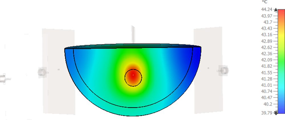
Temperature distributions for the optimized SAR patterns were computed using the bioheat transfer model described in Equation 9. Figures 8 and 9 show the temperature distributions in the breast phantom xy-plane cut, relative to the baseline tissue temperature of  $37^\circ\mathrm{C}$, for the no-GNP case obtained using CST and Python/GA optimization, respectively. In both cases, contour maps were generated using the same optimized excitation amplitudes and phases across all eight ports, with a total input power of 5.75 W and a heating duration of 60 minutes.
Temperature distribution at the xy-plane for baseline scenario without GNPs after 60 minutes of applied EM energy, where the antenna feeding parameters were optimized within CST.

Figure 8 Long description
The plot displays temperature distribution at the xy-plane for a baseline scenario without gold nanoparticles after 60 minutes of applied electromagnetic energy. The domain is semicircular in shape, representing a cross-sectional plane. No axis labels or coordinate units are visible in the image. The colorbar is positioned along the right side of the plot. Numeric values appear to be present on the colorbar, but are not readable at this resolution. The colorbar spans from a lower temperature at the outer boundary of the semicircle to a higher temperature at the central hotspot region. The peak temperature region is located near the center of the flat boundary of the semicircle. Contour bands radiate outward from this central hotspot toward the curved outer boundary, showing a gradual decrease in temperature with increasing radial distance from the peak. The hotspot is concentrated in a small circular region at the center of the flat edge. Moving outward from the hotspot, successive contour bands indicate progressively lower temperatures. The outermost curved boundary region corresponds to the lowest temperature values visible on the colorbar. The colorbar units are not legible at this resolution, so exact temperature values in degrees Celsius or kelvin cannot be confirmed. Numeric colorbar values are present in the image but unreadable at this resolution and no coordinate or spatial unit labels are provided on the plot axes.
Temperature rise in three orthogonal planes (xy, xz, yz) for baseline case without GNPs, computed using Python/GA post-processing.

Figure 9 Long description
The image contains three heatmaps displaying transient temperature distribution in orthogonal planes: xy, xz and yz. Each plot shows a central hotspot with concentric rings indicating temperature gradients. The xy plane is labeled ′XY at z equals 0.0 mm′, the xz plane is labeled ′XZ through target′ and the yz plane is labeled ′YZ through target′. The axes are labeled ′Index′, but specific units are not provided. The color scale on the right serves as a shared legend for all plots, indicating temperature values from 35 to 50. The central hotspot represents the highest temperature, approximately 50, while the outer rings show cooler temperatures, around 35. The plots illustrate symmetry in temperature distribution across the planes, with the xz plane showing a circular pattern and the yz plane displaying an oval shape. These visualizations represent cross-sections of the same temperature field, highlighting differences in shape and symmetry across the planes.
For the baseline scenarios (without GNPs), the tumor region reaches a maximum temperature increase of approximately 7 $^\circ\mathrm{C}$, reaching an absolute temperature of $44^\circ\mathrm{C}$. This lies within the desired therapeutic range for microwave HT. The surrounding fibro-glandular tissue exhibits temperature rises of $3\text{--}4^\circ\mathrm{C}$, while the outer fat layer remains below a $1\text{--}2^\circ\mathrm{C}$ increase. This temperature gradient is favorable, as it enables selective heating of the tumor while minimizing thermal exposure and potential damage to healthy tissues. The Python-based thermal model yields slightly lower peak temperatures than the CST transient solver. This discrepancy stems from the simplified numerical method used in the Python-based thermal calculation.
The introduction of GNPs is expected to further enhance the temperature rise within the target region owing to the increased SAR relative to the baseline case. However, temperature distributions for the GNP-enhanced scenario were not evaluated, as the thermal properties of the nanoparticles were not measured in this study. Nevertheless, these results suggest that GNPs act as effective thermal sensitizers for microwave HT, improving tumor heating selectivity and potentially enhancing therapeutic efficacy compared with conventional EM heating alone.
Conclusion
This study presents a comprehensive numerical investigation of GNP-enhanced microwave HT for breast cancer treatment using a realistic three-layer breast phantom model. Two optimization approaches – Python-based GA post-processing and CST direct optimization – were compared for their ability to maximize SAR focusing in the tumor region with and without GNPs.
The key findings can be summarized as follows:
The introduction of a 5.85 nM concentration of 21 nm GNPs within the tumor resulted in a 65–75% increase in peak SAR values compared to the baseline case without nanoparticles, for the same total input power. The TBQ improved by 39–47% across both optimization methods, demonstrating superior EM energy concentration in the target volume.
The thermal simulations confirmed that GNPs enable achieving therapeutic temperatures (40–45 $^{\circ}$C) with enhanced spatial selectivity. The nanoparticle-loaded region reached therapeutic temperatures while maintaining healthy tissue below critical thresholds, with minimal perturbation to the temperature distribution outside the tumor. The fraction of tumor volume receiving a therapeutically relevant thermal dose increased from 62–68% in the baseline cases to 89–94% with GNPs.
Both the Python/GA post-processing and CST direct optimization approaches achieved effective SAR focusing, with the Python method offering sixfold faster computation (22–24 vs. 145–158 minutes) while the CST method provided marginally better hotspot suppression in healthy tissue (12–15% lower HTQ values). The Python/GA approach is thus more suitable for parametric studies, while CST direct optimization may be preferred when maximal healthy tissue protection is prioritized.
Clinical implications: The FORA antenna array achieves a highly integrated therapeutic effect by serving as the sole external energy source, leveraging the modified dielectric properties of the tumor rather than requiring secondary optical activation. Because the heating mechanism relies on the nanoparticles enhancing local electrical conductivity to boost microwave energy absorption—rather than relying on laser-driven surface plasmon resonance—this single-modality approach completely eliminates the need for separate laser systems, significantly simplifying clinical implementation.
The results support the feasibility of integrating GNPs into microwave HT protocols to enhance treatment selectivity and efficacy. The enhanced SAR focusing and temperature control achieved with GNPs could enable lower input power levels while maintaining therapeutic efficacy, thereby reducing the risk of healthy tissue damage and improving patient safety.
Future work should address several important considerations for clinical translation, including: (i) experimental validation of the numerical predictions using tissue-mimicking phantoms with characterized nanoparticle distributions, (ii) a more extensive parametric study considering different breast anatomies, tumor sizes, and alternative antenna configurations to assess the generality of the proposed approach, and (iii) extension of the optimization framework to incorporate thermal feedback directly into the cost function, replacing the current SAR-based metrics with temperature-based objectives derived from the Pennes bioheat equation, to achieve a controlled and sustained temperature elevation of 5 $^{\circ}$C at the tumor center. This thermally-coupled optimization is expected to resolve the excitation degeneracy observed in the current SAR-based framework and will be developed within the Python/GA architecture, which offers the computational efficiency necessary for iterative thermal evaluation without requiring repeated full EM re-simulation.
In conclusion, this study provides computational evidence that GNPs can significantly enhance the focussability and therapeutic selectivity of microwave HT systems for breast cancer treatment, offering a promising avenue for improving clinical outcomes in adjunctive HT therapy.
Funding statement
This work is financed by Xjenza Malta and the Scientific Technology Research Council (TÜBİTAK) under the Grant Number 123N484, through the Xjenza Malta – TÜBİTAK 2023 Joint Call for R&I projects.
Competing interests
The author(s) declare none.

Iman Farhat received B.Sc. and M.Sc. in Physics from the University of Tripoli and Ph.D. in Physics from the University of Malta in 2015. She is now a Scientific Officer at the University of Malta, working on antenna design and measurements, dielectric spectroscopy, and biomedical electromagnetics applications. Her recent work also includes antenna and analysis pipelines for global 21 cm Cosmic Dawn experiments, with an emphasis on beam characterization, chromaticity mitigation, and sky-beam modeling.

Gulsah Yildiz is an Assistant Professor in the Department of Electronics and Communication Engineering at Istanbul Technical University (ITU). She received her B.Sc. and M.Sc. degrees in Electrical and Electronics Engineering from Bilkent University, and her Ph.D. in Telecommunication Engineering from ITU. Her research focuses on personalized medical device development, including microwave hyperthermia, microwave imaging, high-intensity focused ultrasound, and AI-driven treatment personalization. She has led and contributed to several nationally and internationally funded projects on cancer therapy technologies, dielectric imaging, and medical device development.

Federico Cilia earned a B.Eng. (Hons) in electrical and electronics in 2019, followed by an M.Sc. in Engineering (Electrical) in 2021, both from the University of Malta. From 2021 to 2025, he worked on the MiTreat project as a research support officer. He currently serves as a Research Support Officer at the University of Malta, contributing to the ABLAZE project while pursuing a Ph.D. at the same institution. His current research interests include radiofrequency and electromagnetic engineering, dielectric spectroscopy of biological tissues for medical applications, computational electromagnetics, as well as antenna design and engineering.

Julian Bonello earned his B.Sc. (Hons) in Physics and Computing (2012) and an M.Sc. in Physics (2015) from the University of Malta. Upon completing his master’s degree, he joined the Physics Department’s Electromagnetics Laboratory as a researcher. In 2020, he was conferred a Ph.D. by the same institution, following his doctoral research on the complex permittivity variations of biological tissues across temperature and frequency spectra. His current research focuses on the development of instrumentation and measurement.

Francesco Rossi held the position of honorary researcher at UCL from 2026, where he received a Ph.D. in Biophysics and Nanotechnology in 2020. He earned his B.Sc. and M.Sc. at the University of Florence, and in 2021 and 2022, he held the position of lecturer of Chemistry for the international students of Ca’Foscari University (Venice, Italy). Between 2024 and 2025, he was a postdoc researcher at the Institute for the Chemistry of Organometallic Compounds (ICCOM) of the Consiglio Nazionale delle Ricerche (CNR, Italy). His research is focused on the application of nanomaterials to different fields of everyday life, from nanomedicine to self-sterilizing surfaces.

Nguyen Thi Kim Thanh held a prestigious Royal Society University Research Fellowship (2005–2014) and was appointed Full Professor in Nanomaterials in 2013 at University College London. Currently, she is Vice Dean for Innovation and Enterprise at UCL’s faculty of mathematical and physical sciences. In 2019, Professor Thanh was honored for her achievements in the field of nanomaterials, and her impactful project proposal was awarded the prestigious Royal Society Rosalind Franklin Medal. She was awarded the RSC/SCI 2023 Graham Prize Lectureship. Professor Thanh is Editor-in-Chief of the RSC book series Nanoscience & Nanotechnology. She has edited several themed issues. She was a member of the Joint Committee of the RSC Colloid & Interface Science Group and SCI Colloid & Surface Chemistry Group (2008–2017). She was also a representative member of the Joint Colloids Groups at the RSC Faraday Division Council (2013–2016).

Charles Sammut holds a B.A. in Education from University of Malta (UM) (1980), a B.Sc. in Physics with Physical Electronics (graduating with First Class Honours in 1987, when he was also awarded the British Aerospace Prize for Physics), and a Ph.D. in the field of microwave semiconductor devices (1992) from the University of Bath, UK, from where he received the Deryck Chesterman for outstanding research leading to his Ph.D. He is currently a full Professor at the Department of Physics, UM, which he headed between 1997 and 2000 and again from 2007 to 2019, during which period he was also Dean of the Faculty of Science. His current research interests include: dielectric spectroscopy of biological tissues for medical applications; microwave measurements; computational electromagnetics; antenna design; exposure of workers and the general public to non-ionizing electromagnetic fields; biological effects of non-ionizing electromagnetic fields, and he has published extensively on these topics.

Lourdes Farrugia received her M.Sc. and Ph.D. in Physics from the University of Malta in 2008 and 2016, respectively. She is an Associate Professor and head of the Physics Department at the University of Malta. Her research interests comprise aspects of instrumentation and measurement of dielectric properties, in particular those of biological tissues, as relevant to the microwave medical device community. Dr Farrugia was the chair of COST Action CA17115 MyWAVE. She is a member of the Technical Advisory Committee of URSI Commission K and a member of the ASME Thermal Medicine Committee.







 Open access

