


1. Introduction
Signatures play an important and unique role in reliability theory [Reference Da and Ding6, Reference Samaniego18]. Their theory has developed considerably since the first notion called “system signature” was proposed by Samaniego [Reference Samaniego17] as  $\boldsymbol{s}=(s_1,\ldots,s_n)$ for coherent systems with
  $n$ components which are independent and identically distributed (i.i.d.) from a continuous-time distribution; here,
  $s_i$ is the probability that the
  $i$th component failure causes the failure of the system. Various signature measures have been proposed for describing structural properties of different types of coherent systems. These include joint signature for coherent systems with shared components [Reference Navarro, Samaniego and Balakrishnan15, Reference Navarro, Samaniego and Balakrishnan16], dynamic signature for used coherent systems with known number of failed components [Reference Samaniego, Balakrishnan and Navarro19], minimal/maximal signature for coherent systems with exchangeable components [Reference Navarro, Ruiz and Sandoval14], survival signature for coherent systems with multiple types of components [Reference Coolen, Coolen-Maturi, Zamojski, Mazurkiewicz, Sugier, Walkowiak and Kacprzyk5], ordered signature for coherent systems in a life-test of systems [Reference Balakrishnan and Volterman2, Reference Yi, Balakrishnan and Li25], and their counterparts for multi-state coherent systems [Reference Yi, Balakrishnan and Cui22–Reference Yi, Balakrishnan and Li24, Reference Yi, Balakrishnan and Li26, Reference Yi, Balakrishnan and Li27]. A detailed review of these has been provided in [Reference Yi, Balakrishnan, Liu, Wang, Mi and Li21].
In practical reliability systems, it is common to see components shared by different systems, which leads to the concept of joint signature. Navarro et al. [Reference Navarro, Samaniego and Balakrishnan15] originally tried to define joint signature based on joint distribution of the systems with shared components, and Navarro et al. [Reference Navarro, Samaniego and Balakrishnan16] argued subsequently that it will be better to define the joint signature to be  $\boldsymbol{s}=(s_{i,j},{\rm{~}}1\le i,j\le n)$; here,
  $s_{i,j}$ is the probability that the
  $i$th and
  $j$th component failures cause the two systems to fail, respectively. More discussions can be found with regard to statistical inference in [Reference Balakrishnan and Volterman3], generalizations to two or more systems in [Reference Marichal, Mathonet, Navarro and Paroissin13] and [Reference Zarezadeh, Mohammadi and Balakrishnan29], and some others in [Reference Yi, Balakrishnan and Li24, Reference Yi, Balakrishnan and Li27, Reference Yi, Balakrishnan and Li28].
Signatures are quite useful in describing structures of various reliability systems and in studying their lifetime properties. However, one of the main limitations in the associated theory is that it is based on the assumption that component lifetimes follow a continuous-time distribution, while many practical reliability systems actually have their component lifetimes to be discrete [Reference Baik and Cho1, Reference Dembinska and Eryilmaz7–Reference Hu, Hu, Wu and Yu12, Reference Shaked, Shanthikumar, Valdez-Torres and Özekici20]. For this reason, Balakrishnan et al. [Reference Balakrishnan, Yi and Goroncy4] recently generalized the Samaniego’s [Reference Samaniego17] notion of system signature to discrete-time signature and discussed some of its stochastic properties. In the present work, we further develop joint signature when the component lifetimes follow a discrete-time distribution, in analogy to the work of Navarro et al. [Reference Navarro, Samaniego and Balakrishnan15, Reference Navarro, Samaniego and Balakrishnan16] on joint signature for systems with components possessing a continuous lifetime distribution.
The rest of this paper proceeds as follows. In Section 2, we introduce the definition of discrete-time joint signature for two coherent systems with shared components, whose lifetimes are i.i.d. from a discrete-time distribution, and the joint distribution of the system lifetimes is discussed in detail. In Section 3, some series and parallel systems with shared components are studied based on their discrete-time joint signature for a clear understanding of the concept. In Section 4, stochastic ordering results are presented for two pairs of coherent systems with some shared components. In Section 5, a transformation formula is introduced for pairs of systems of different sizes so that they can be stochastically compared. Some concluding remarks are finally made in Section 6.
2. Joint signature and joint distribution of system lifetimes
In the continuous-time case, Navarro et al. [Reference Navarro, Samaniego and Balakrishnan16] defined joint signature for two coherent systems  $\phi_1,\phi_2$ with
  $n$ shared components, whose lifetimes
  $X_1,\ldots,X_n$ are i.i.d. continuous random variables, as
  $\boldsymbol{s}=(s_{i,j},{\rm{~}},1\le i,j\le n)$ with its
  $(i,j)$-th element
  $s_{i,j}=P\{T_1=X_{i:n},{\rm{~}}T_2=X_{j:n}\}$, where
  $T_1$ and
  $T_2$ are the lifetimes of systems
  $\phi_1,\phi_2$, and
  $X_{1:n} \le \cdots \le X_{n:n}$ are the order statistics corresponding to the component lifetimes
  $X_1,\ldots,X_n$. Now, along the lines of Balakrishnan et al. [Reference Balakrishnan, Yi and Goroncy4], the concept of joint signature in the discrete-time case is introduced as follows.
Definition 2.1. For two coherent systems  $\phi_1,\phi_2$ with
  $n$ shared components and lifetimes
  $T_1,T_2$, suppose the components have i.i.d. discrete lifetimes
  ${X_1}, \ldots ,{X_n}$ from a cumulative distribution function (cdf)
  $F(\cdot)$ and a probability mass function (pmf)
  $f(\cdot)$. Let us denote the
  $i$-th smallest component lifetime by
  ${X_{i:n}}$. Then, the joint signature of the two systems can be defined as
 \begin{equation*}{\boldsymbol{s}} = \left( {{s_{i_1,i_2}^{\,j_1,\ldots,j_{m}}},{\rm{~}} j_1 +\cdots +j_m= n,{\rm{~}}1\le i_1,i_2\le m\le n} \right),\end{equation*}
where
 \begin{equation*}{s_{i_1,i_2}^{\,j_1,\ldots,j_m}} = P\{T_1 = {X_{j_{(i_1-1)}+1 :n}},{\rm{~}}T_2 = {X_{j_{(i_2-1)}+1 :n}}\left|{{E_{j_1,\ldots,j_m}}}\right.\} \end{equation*}
is the conditional probability that failure of System  $\phi_1$ is caused by the
  $(j_{(i_1-1)}+1)$-th component failure and failure of System
  $\phi_2$ is caused by the
  $(j_{(i_2-1)}+1)$-th component failure, given the event
 \begin{equation*}{E_{j_1,\ldots,j_m}}=\{X_{(1,\ldots,j_{(1)}):n} \lt {X_{(j_{(1)}+1,\ldots,j_{(2)}):n}} \lt \cdots \lt {X_{(j_{(m-1)} +1,\ldots,j_{(m)} ):n}}\};\end{equation*}
here,  ${j_1},\ldots,{j_m}$ are the numbers of order statistics
  $X_{1:n},\ldots,X_{n:n}$ that are equal to the first, second,
  $\ldots$,
  $m$-th distinct values, respectively. We use
  ${X_{(u,\ldots,v):n}}$ as an abbrevation for
  ${X_{u:n}}=\cdots={X_{v:n}}$ (
 $1\le u \le v\le n$) and
  $j_{(i)}={j_1}+\cdots+{j_i}$ for the
  $i$-th patial sum, for
  $i=1,\ldots,m$. It is evident that
  $j_{(1)}=j_1$ and
  $j_{(m)}=\sum\nolimits_{i=1}^{m} {j_i} =n$. For convenience, we set
  $j_{(0)}=0$ and
  $j_{(-1)} =-1$.
Remark 2.1. It is useful to observe that the discrete-time joint signature is distribution-free, namely, the elements  ${s_{i_1,i_2}^{\,j_1,\ldots,j_m}}$ do not depend on the components’ lifetime distribution
  $F$. Besides,
 \begin{equation*}\sum\limits_{i_1=1}^m\sum\limits_{i_2=1}^m{s_{i_1,i_2}^{\,j_1,\ldots,j_m}}=1\end{equation*}
holds for all  $j_1 +\cdots +j_m= n$ (
 $1\le m\le n$), which is due to the fact that the discrete-time joint signature has been defined based on conditional event
  ${E_{j_1,\ldots,j_m}}$. If not, we can redefine the discrete-time joint signature in an unconditional way as
 \begin{equation*}{s_{i_1,i_2}^{\,j_1,\ldots,j_m}} = P\{T_1 = {X_{j_{(i_1-1)}+1 :n}},{\rm{~}}T_2 = {X_{j_{(i_2-1)}+1 :n}},{\rm{~}}{E_{j_1,\ldots,j_m}}\} ,\end{equation*}
which would lead to 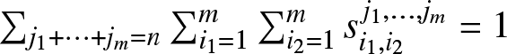 $\sum\nolimits_{j_1 +\cdots +j_m= n}\sum\nolimits_{i_1=1}^m\sum\nolimits_{i_2=1}^m{s_{i_1,i_2}^{\,j_1,\ldots,j_m}}=1$ instead.
Remark 2.2. The discrete-time joint signature can be regarded as a matrix of dimension  $C_n\times n^2$, where
  $C_n=\sum\limits_{m = 1}^n {\left( {\begin{matrix}
{n - 1} \\
{m - 1} \end{matrix} } \right)}=2^{n-1} $ is the total number of compositions (i.e., distinguishable partitions) of an integer
$C_n=\sum\limits_{m = 1}^n {\left( {\begin{matrix}
{n - 1} \\
{m - 1} \end{matrix} } \right)}=2^{n-1} $ is the total number of compositions (i.e., distinguishable partitions) of an integer  $n$. For example, in the case of
  $n=2$, there are
  $C_2=2^{2-1}=2$ possible compositions, that is,
  $j_1=j_2=1$ and
  $j_1=2$. The first composition
  $j_1=j_2=1$ corresponds to the first row of
  $\boldsymbol{s}$, that is,
  $s^{1,1}_{i_1,i_2},{\rm{~}}1\le i_1,i_2\le 2$; and the second composition
  $j_1=2$ corresponds to the second row of
  $\boldsymbol{s}$, that is,
  $s^{1,1}_{i_1,i_2},{\rm{~}}1\le i_1,i_2\le 1$; see Example 3.1 for pertinent details. Similar discussions can also be provided for
  $n=3$; see Example 3.2 for details.
The above definition of joint signature can be used readily to present the following expressions concerning the joint distribution of system lifetimes.
Proposition 2.1. The joint pmf of the system lifetimes  $T_1,T_2$ can be given as
 \begin{equation*}P\{T_1 = x,{\rm{~}}T_2=y\} = \sum\limits_{m=1}^n\sum\limits_{j_1 +\cdots +j_m= n}\left( {\begin{matrix}
n \\
{j_1,\ldots,j_m} \end{matrix} } \right) {\sum\limits_{i _1= 1}^{m}\sum\limits_{i _2= 1}^{m} {{s_{i_1,i_2}^{\,j_1,\ldots,j_m}} \left[ \sum\limits_{\scriptstyle 1 \le {t_1} \lt \cdots \lt {t_m} \lt \infty, \atop \!\!\!\!\!\!\!\!\!\!\!\!\!\!\!\!\!\!\!\!\!\scriptstyle t_{i_1}= x,{\rm{~}}t_{i_2}=y } {{\prod\limits_{u = 1}^m {{f^{{j_u}}}({t_u})} } } \right] } },\end{equation*}
\begin{equation*}P\{T_1 = x,{\rm{~}}T_2=y\} = \sum\limits_{m=1}^n\sum\limits_{j_1 +\cdots +j_m= n}\left( {\begin{matrix}
n \\
{j_1,\ldots,j_m} \end{matrix} } \right) {\sum\limits_{i _1= 1}^{m}\sum\limits_{i _2= 1}^{m} {{s_{i_1,i_2}^{\,j_1,\ldots,j_m}} \left[ \sum\limits_{\scriptstyle 1 \le {t_1} \lt \cdots \lt {t_m} \lt \infty, \atop \!\!\!\!\!\!\!\!\!\!\!\!\!\!\!\!\!\!\!\!\!\scriptstyle t_{i_1}= x,{\rm{~}}t_{i_2}=y } {{\prod\limits_{u = 1}^m {{f^{{j_u}}}({t_u})} } } \right] } },\end{equation*}the joint survival function as
 \begin{align*}
P\{T_1 \gt x,{\rm{~}}T_2 \gt y\} =& \sum\limits_{m=1}^n\sum\limits_{j_1 +\cdots +j_m= n}\left( {\begin{matrix}
n \\
{j_1,\ldots,j_m} \end{matrix} } \right)
\sum\limits_{i_1=0}^{m-1}\sum\limits_{i_2=0}^{m-1}\bar S_{i_1,i_2}^{\,j_1,\ldots,j_m}\left[ \sum\limits_{\!\!\!\!\!\!\!\!\!\!\!\!\!\!\!\!\!\!\!\!\!\!\!\scriptstyle 1 \le {t_1} \lt \cdots \lt {t_m} \lt \infty, \atop
\scriptstyle t_{i_1}\le x \lt t_{i_1+1}, {\rm{~}} t_{i_2}\le y \lt t_{i_2+1} } {{\prod\limits_{u = 1}^m {{f^{{j_u}}}({t_u})} } } \right],
\end{align*}
\begin{align*}
P\{T_1 \gt x,{\rm{~}}T_2 \gt y\} =& \sum\limits_{m=1}^n\sum\limits_{j_1 +\cdots +j_m= n}\left( {\begin{matrix}
n \\
{j_1,\ldots,j_m} \end{matrix} } \right)
\sum\limits_{i_1=0}^{m-1}\sum\limits_{i_2=0}^{m-1}\bar S_{i_1,i_2}^{\,j_1,\ldots,j_m}\left[ \sum\limits_{\!\!\!\!\!\!\!\!\!\!\!\!\!\!\!\!\!\!\!\!\!\!\!\scriptstyle 1 \le {t_1} \lt \cdots \lt {t_m} \lt \infty, \atop
\scriptstyle t_{i_1}\le x \lt t_{i_1+1}, {\rm{~}} t_{i_2}\le y \lt t_{i_2+1} } {{\prod\limits_{u = 1}^m {{f^{{j_u}}}({t_u})} } } \right],
\end{align*}and the joint cdf as
 \begin{align*}
P\{T_1 \le x,{\rm{~}}T_2 \le y\} =& \sum\limits_{m=1}^n\sum\limits_{j_1 +\cdots +j_m= n}\left( {\begin{matrix}
n \\
{j_1,\ldots,j_m} \end{matrix} } \right)
\sum\limits_{i_1=1}^{m}\sum\limits_{i_2=1}^{m} S_{i_1,i_2}^{\,j_1,\ldots,j_m} \left[ \sum\limits_{\!\!\!\!\!\!\!\!\!\!\!\!\!\!\!\!\!\!\!\!\!\!\!\scriptstyle 1 \le {t_1} \lt \cdots \lt {t_m} \lt \infty, \atop \scriptstyle t_{i_1}\le x \lt t_{i_1+1}, {\rm{~}} t_{i_2}\le y \lt t_{i_2+1} } {{\prod\limits_{u = 1}^m {{f^{{j_u}}}({t_u})} } } \right],
\end{align*}
\begin{align*}
P\{T_1 \le x,{\rm{~}}T_2 \le y\} =& \sum\limits_{m=1}^n\sum\limits_{j_1 +\cdots +j_m= n}\left( {\begin{matrix}
n \\
{j_1,\ldots,j_m} \end{matrix} } \right)
\sum\limits_{i_1=1}^{m}\sum\limits_{i_2=1}^{m} S_{i_1,i_2}^{\,j_1,\ldots,j_m} \left[ \sum\limits_{\!\!\!\!\!\!\!\!\!\!\!\!\!\!\!\!\!\!\!\!\!\!\!\scriptstyle 1 \le {t_1} \lt \cdots \lt {t_m} \lt \infty, \atop \scriptstyle t_{i_1}\le x \lt t_{i_1+1}, {\rm{~}} t_{i_2}\le y \lt t_{i_2+1} } {{\prod\limits_{u = 1}^m {{f^{{j_u}}}({t_u})} } } \right],
\end{align*}where  $t_0=0$,
 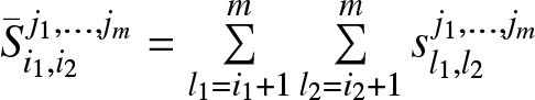 $\bar S_{i_1,i_2}^{\,j_1,\ldots,j_m}=\sum\limits_{l_1 = i_1+1}^{m}\sum\limits_{l_2 = i_2+1}^{m} {s_{l_1,l_2}^{\,j_1,\ldots,j_m}}$ and
  $S_{i_1,i_2}^{\,j_1,\ldots,j_m}=\sum\limits_{l_1 = 1}^{i_1}\sum\limits_{l_2 = 1}^{i_2} {s_{l_1,l_2}^{\,j_1,\ldots,j_m}}$.
Proof. According to Definition 2.1, we have
 \begin{align*}
& P\{T_1 = x,{\rm{~}}T_2=y\} \\
=& \sum\limits_{m=1}^n\sum\limits_{j_1 +\cdots +j_m= n} {\sum\limits_{i_1 = 1}^{m}\sum\limits_{i_2 = 1}^{m} {P\{T_1 =x,{\rm{~}}T_2=y\left|T_1 = {X_{j_{(i_1-1)}+1 :n}},{\rm{~}}T_2 = {X_{j_{(i_2-1)}+1 :n}},{\rm{~}}E_{j_1,\ldots,j_m}\right.\} } } \\
&\times P\{T_1 = {X_{j_{(i_1-1)}+1 :n}},{\rm{~}}T_2 = {X_{j_{(i_2-1)}+1 :n}},{\rm{~}}{E_{j_1,\ldots,j_m}}\} \end{align*}
\begin{align*}
& P\{T_1 = x,{\rm{~}}T_2=y\} \\
=& \sum\limits_{m=1}^n\sum\limits_{j_1 +\cdots +j_m= n} {\sum\limits_{i_1 = 1}^{m}\sum\limits_{i_2 = 1}^{m} {P\{T_1 =x,{\rm{~}}T_2=y\left|T_1 = {X_{j_{(i_1-1)}+1 :n}},{\rm{~}}T_2 = {X_{j_{(i_2-1)}+1 :n}},{\rm{~}}E_{j_1,\ldots,j_m}\right.\} } } \\
&\times P\{T_1 = {X_{j_{(i_1-1)}+1 :n}},{\rm{~}}T_2 = {X_{j_{(i_2-1)}+1 :n}},{\rm{~}}{E_{j_1,\ldots,j_m}}\} \end{align*} \begin{align*}
=& \sum\limits_{m=1}^n\sum\limits_{j_1 +\cdots +j_m= n} {\sum\limits_{i_1 = 1}^{m} \sum\limits_{i_2 = 1}^{m}{P\{{X_{j_{(i_1-1)}+1 :n}} =x,{\rm{~}}{X_{j_{(i_2-1)}+1 :n}} =y\left|E_{j_1,\ldots,j_m}\right.\} } } \cdot {s_{i_1,i_2}^{\,j_1,\ldots,j_m}} \cdot P\{E_{j_1,\ldots,j_m}\} \\
=& \sum\limits_{m=1}^n\sum\limits_{j_1 +\cdots +j_m= n} {\sum\limits_{i_1 = 1}^{m}\sum\limits_{i_2 = 1}^{m} {{s_{i_1,i_2}^{\,j_1,\ldots,j_m}} \cdot P\{{X_{j_{(i_1-1)}+1 :n}} =x,{\rm{~}}{X_{j_{(i_2-1)}+1 :n}} =y,{\rm{~}} E_{j_1,\ldots,j_m}\} } }.
\end{align*}
\begin{align*}
=& \sum\limits_{m=1}^n\sum\limits_{j_1 +\cdots +j_m= n} {\sum\limits_{i_1 = 1}^{m} \sum\limits_{i_2 = 1}^{m}{P\{{X_{j_{(i_1-1)}+1 :n}} =x,{\rm{~}}{X_{j_{(i_2-1)}+1 :n}} =y\left|E_{j_1,\ldots,j_m}\right.\} } } \cdot {s_{i_1,i_2}^{\,j_1,\ldots,j_m}} \cdot P\{E_{j_1,\ldots,j_m}\} \\
=& \sum\limits_{m=1}^n\sum\limits_{j_1 +\cdots +j_m= n} {\sum\limits_{i_1 = 1}^{m}\sum\limits_{i_2 = 1}^{m} {{s_{i_1,i_2}^{\,j_1,\ldots,j_m}} \cdot P\{{X_{j_{(i_1-1)}+1 :n}} =x,{\rm{~}}{X_{j_{(i_2-1)}+1 :n}} =y,{\rm{~}} E_{j_1,\ldots,j_m}\} } }.
\end{align*} Similarly, with the convention that  $X_{0:n}=0$, we have
 \begin{align*}
& P\{T_1 \gt x,{\rm{~}}T_2 \gt y\} \\
=& \sum\limits_{m=1}^n\sum\limits_{j_1 +\cdots +j_m= n} {\sum\limits_{l_1 = 1}^{m}\sum\limits_{l_2 = 1}^{m} {P\{T_1 \gt x,{\rm{~}}T_2 \gt y\left|T_1 = {X_{j_{(l_1-1)}+1 :n}},{\rm{~}}T_2 = {X_{j_{(l_2-1)}+1 :n}},{\rm{~}}E_{j_1,\ldots,j_m}\right.\} } } \\
&\times P\{T_1 = {X_{j_{(l_1-1)}+1 :n}},{\rm{~}}T_2 = {X_{j_{(l_2-1)}+1 :n}},{\rm{~}}{E_{j_1,\ldots,j_m}}\} \\
=& \sum\limits_{m=1}^n\sum\limits_{j_1 +\cdots +j_m= n} {\sum\limits_{l_1 = 1}^{m}\sum\limits_{l_2 = 1}^{m} {P\{{X_{j_{(l_1-1)} +1:n}} \gt x,{\rm{~}}{X_{j_{(l_2-1)} +1:n}} \gt y\left|E_{j_1,\ldots,j_m}\right.\} } } \cdot {s_{l_1,l_2}^{\,j_1,\ldots,j_m}} \cdot P\{E_{j_1,\ldots,j_m}\} \\
=& \sum\limits_{m=1}^n\sum\limits_{j_1 +\cdots +j_m= n} {\sum\limits_{l_1 = 1}^{m}\sum\limits_{l_2 = 1}^{m} {{s_{l_1,l_2}^{\,j_1,\ldots,j_m}} \cdot P\{{X_{j_{(l_1-1)}+1 :n}} \gt x,{\rm{~}}{X_{j_{(l_2-1)}+1 :n}} \gt y,{\rm{~}} E_{j_1,\ldots,j_m}\} } }\\
=& \sum\limits_{m=1}^n\sum\limits_{j_1 +\cdots +j_m= n} {\sum\limits_{l_1 = 1}^{m}\sum\limits_{l_2 = 1}^{m} {{s_{l_1,l_2}^{\,j_1,\ldots,j_m}} \cdot \sum\limits_{i_1=0}^{l_1-1}\sum\limits_{i_2=0}^{l_2-1}P\{{X_{j_{(i_1-1)}+1 :n}} \le x \lt {X_{j_{(i_1)}+1 :n}},{\rm{~}}{X_{j_{(i_2-1)}+1 :n}} \le y \lt } }\\
&{X_{j_{(i_2)}+1 :n}},{\rm{~}} E_{j_1,\ldots,j_m}\} \\
=& \sum\limits_{m=1}^n\sum\limits_{j_1 +\cdots +j_m= n}
\sum\limits_{i_1=0}^{m-1}\sum\limits_{i_2=0}^{m-1} \left(\sum\limits_{l_1 = i_1+1}^{m}\sum\limits_{l_2 = i_2+1}^{m} {s_{l_1,l_2}^{\,j_1,\ldots,j_m}}\right) \cdot P\{{X_{j_{(i_1-1)} +1:n}} \le x \lt {X_{j_{(i_1)}+1 :n}},{\rm{~}}{X_{j_{(i_2-1)} +1:n}} \\
&\le y \lt {X_{j_{(i_2)}+1 :n}},{\rm{~}} E_{j_1,\ldots,j_m}\} .
\end{align*}
\begin{align*}
& P\{T_1 \gt x,{\rm{~}}T_2 \gt y\} \\
=& \sum\limits_{m=1}^n\sum\limits_{j_1 +\cdots +j_m= n} {\sum\limits_{l_1 = 1}^{m}\sum\limits_{l_2 = 1}^{m} {P\{T_1 \gt x,{\rm{~}}T_2 \gt y\left|T_1 = {X_{j_{(l_1-1)}+1 :n}},{\rm{~}}T_2 = {X_{j_{(l_2-1)}+1 :n}},{\rm{~}}E_{j_1,\ldots,j_m}\right.\} } } \\
&\times P\{T_1 = {X_{j_{(l_1-1)}+1 :n}},{\rm{~}}T_2 = {X_{j_{(l_2-1)}+1 :n}},{\rm{~}}{E_{j_1,\ldots,j_m}}\} \\
=& \sum\limits_{m=1}^n\sum\limits_{j_1 +\cdots +j_m= n} {\sum\limits_{l_1 = 1}^{m}\sum\limits_{l_2 = 1}^{m} {P\{{X_{j_{(l_1-1)} +1:n}} \gt x,{\rm{~}}{X_{j_{(l_2-1)} +1:n}} \gt y\left|E_{j_1,\ldots,j_m}\right.\} } } \cdot {s_{l_1,l_2}^{\,j_1,\ldots,j_m}} \cdot P\{E_{j_1,\ldots,j_m}\} \\
=& \sum\limits_{m=1}^n\sum\limits_{j_1 +\cdots +j_m= n} {\sum\limits_{l_1 = 1}^{m}\sum\limits_{l_2 = 1}^{m} {{s_{l_1,l_2}^{\,j_1,\ldots,j_m}} \cdot P\{{X_{j_{(l_1-1)}+1 :n}} \gt x,{\rm{~}}{X_{j_{(l_2-1)}+1 :n}} \gt y,{\rm{~}} E_{j_1,\ldots,j_m}\} } }\\
=& \sum\limits_{m=1}^n\sum\limits_{j_1 +\cdots +j_m= n} {\sum\limits_{l_1 = 1}^{m}\sum\limits_{l_2 = 1}^{m} {{s_{l_1,l_2}^{\,j_1,\ldots,j_m}} \cdot \sum\limits_{i_1=0}^{l_1-1}\sum\limits_{i_2=0}^{l_2-1}P\{{X_{j_{(i_1-1)}+1 :n}} \le x \lt {X_{j_{(i_1)}+1 :n}},{\rm{~}}{X_{j_{(i_2-1)}+1 :n}} \le y \lt } }\\
&{X_{j_{(i_2)}+1 :n}},{\rm{~}} E_{j_1,\ldots,j_m}\} \\
=& \sum\limits_{m=1}^n\sum\limits_{j_1 +\cdots +j_m= n}
\sum\limits_{i_1=0}^{m-1}\sum\limits_{i_2=0}^{m-1} \left(\sum\limits_{l_1 = i_1+1}^{m}\sum\limits_{l_2 = i_2+1}^{m} {s_{l_1,l_2}^{\,j_1,\ldots,j_m}}\right) \cdot P\{{X_{j_{(i_1-1)} +1:n}} \le x \lt {X_{j_{(i_1)}+1 :n}},{\rm{~}}{X_{j_{(i_2-1)} +1:n}} \\
&\le y \lt {X_{j_{(i_2)}+1 :n}},{\rm{~}} E_{j_1,\ldots,j_m}\} .
\end{align*} Finally, with the convention that  $X_{n+1:n}=\infty$, we have
 \begin{align*}
& P\{T_1 \le x,{\rm{~}}T_2 \le y\} \\
=& \sum\limits_{m=1}^n\sum\limits_{j_1 +\cdots +j_m= n} {\sum\limits_{l_1 = 1}^{m}\sum\limits_{l_2 = 1}^{m} {P\{T _1\le x,{\rm{~}}T_2 \le y\left|T_1 = {X_{j_{(l_1-1)}+1 :n}},{\rm{~}}T_2 = {X_{j_{(l_2-1)}+1 :n}},{\rm{~}}E_{j_1,\ldots,j_m}\right.\} } } \\
&\times P\{T_1 = {X_{j_{(l_1-1)}+1 :n}},{\rm{~}}T_2= {X_{j_{(l_2-1)}+1 :n}},{\rm{~}}{E_{j_1,\ldots,j_m}}\} \\
=& \sum\limits_{m=1}^n\sum\limits_{j_1 +\cdots +j_m= n} {\sum\limits_{l_1 = 1}^{m} \sum\limits_{l_2 = 1}^{m}{P\{{X_{j_{(l_1-1)}+1 :n}} \le x,{\rm{~}}{X_{j_{(l_2-1)}+1 :n}} \le y\left|E_{j_1,\ldots,j_m}\right.\} } } \cdot {s_{l_1,l_2}^{\,j_1,\ldots,j_m}} \cdot P\{E_{j_1,\ldots,j_m}\} \\
=& \sum\limits_{m=1}^n\sum\limits_{j_1 +\cdots +j_m= n} {\sum\limits_{l_1 = 1}^{m}\sum\limits_{l_2 = 1}^{m} {{s_{l_1,l_2}^{\,j_1,\ldots,j_m}} \cdot P\{{X_{j_{(l_1-1)}+1 :n}} \le x,{\rm{~}}{X_{j_{(l_2-1)}+1 :n}} \le y,{\rm{~}} E_{j_1,\ldots,j_m}\} } }\end{align*}
\begin{align*}
& P\{T_1 \le x,{\rm{~}}T_2 \le y\} \\
=& \sum\limits_{m=1}^n\sum\limits_{j_1 +\cdots +j_m= n} {\sum\limits_{l_1 = 1}^{m}\sum\limits_{l_2 = 1}^{m} {P\{T _1\le x,{\rm{~}}T_2 \le y\left|T_1 = {X_{j_{(l_1-1)}+1 :n}},{\rm{~}}T_2 = {X_{j_{(l_2-1)}+1 :n}},{\rm{~}}E_{j_1,\ldots,j_m}\right.\} } } \\
&\times P\{T_1 = {X_{j_{(l_1-1)}+1 :n}},{\rm{~}}T_2= {X_{j_{(l_2-1)}+1 :n}},{\rm{~}}{E_{j_1,\ldots,j_m}}\} \\
=& \sum\limits_{m=1}^n\sum\limits_{j_1 +\cdots +j_m= n} {\sum\limits_{l_1 = 1}^{m} \sum\limits_{l_2 = 1}^{m}{P\{{X_{j_{(l_1-1)}+1 :n}} \le x,{\rm{~}}{X_{j_{(l_2-1)}+1 :n}} \le y\left|E_{j_1,\ldots,j_m}\right.\} } } \cdot {s_{l_1,l_2}^{\,j_1,\ldots,j_m}} \cdot P\{E_{j_1,\ldots,j_m}\} \\
=& \sum\limits_{m=1}^n\sum\limits_{j_1 +\cdots +j_m= n} {\sum\limits_{l_1 = 1}^{m}\sum\limits_{l_2 = 1}^{m} {{s_{l_1,l_2}^{\,j_1,\ldots,j_m}} \cdot P\{{X_{j_{(l_1-1)}+1 :n}} \le x,{\rm{~}}{X_{j_{(l_2-1)}+1 :n}} \le y,{\rm{~}} E_{j_1,\ldots,j_m}\} } }\end{align*} \begin{align*}
=& \sum\limits_{m=1}^n\sum\limits_{j_1 +\cdots +j_m= n} {\sum\limits_{l_1 = 1}^{m}\sum\limits_{l_2 = 1}^{m} {{s_{l_1,l_2}^{\,j_1,\ldots,j_m}} \cdot \sum\limits_{i_1=l_1}^{m}\sum\limits_{i_2=l_2}^{m}P\{{X_{j_{(i_1-1)} +1:n}} \le x \lt {X_{j_{(i_1)}+1 :n}},{\rm{~}}{X_{j_{(i_2-1)} +1:n}} \le y \lt } }\\
&{X_{j_{(i_2)}+1 :n}},{\rm{~}} E_{j_1,\ldots,j_m}\}\\
=& \sum\limits_{m=1}^n\sum\limits_{j_1 +\cdots +j_m= n}
\sum\limits_{i_1=1}^{m}\sum\limits_{i_2=1}^{m} \left(\sum\limits_{l_1 = 1}^{i_1}\sum\limits_{l_2 = 1}^{i_2} {s_{l_1,l_2}^{\,j_1,\ldots,j_m}}\right) \cdot P\{{X_{j_{(i_1-1)}+1 :n}} \le x \lt {X_{j_{(i_1)}+1 :n}},{\rm{~}}{X_{j_{(i_2-1)}+1 :n}} \le y
\\
& \lt {X_{j_{(i_2)}+1 :n}},{\rm{~}} E_{j_1,\ldots,j_m}\} .
\end{align*}
\begin{align*}
=& \sum\limits_{m=1}^n\sum\limits_{j_1 +\cdots +j_m= n} {\sum\limits_{l_1 = 1}^{m}\sum\limits_{l_2 = 1}^{m} {{s_{l_1,l_2}^{\,j_1,\ldots,j_m}} \cdot \sum\limits_{i_1=l_1}^{m}\sum\limits_{i_2=l_2}^{m}P\{{X_{j_{(i_1-1)} +1:n}} \le x \lt {X_{j_{(i_1)}+1 :n}},{\rm{~}}{X_{j_{(i_2-1)} +1:n}} \le y \lt } }\\
&{X_{j_{(i_2)}+1 :n}},{\rm{~}} E_{j_1,\ldots,j_m}\}\\
=& \sum\limits_{m=1}^n\sum\limits_{j_1 +\cdots +j_m= n}
\sum\limits_{i_1=1}^{m}\sum\limits_{i_2=1}^{m} \left(\sum\limits_{l_1 = 1}^{i_1}\sum\limits_{l_2 = 1}^{i_2} {s_{l_1,l_2}^{\,j_1,\ldots,j_m}}\right) \cdot P\{{X_{j_{(i_1-1)}+1 :n}} \le x \lt {X_{j_{(i_1)}+1 :n}},{\rm{~}}{X_{j_{(i_2-1)}+1 :n}} \le y
\\
& \lt {X_{j_{(i_2)}+1 :n}},{\rm{~}} E_{j_1,\ldots,j_m}\} .
\end{align*}In the above expressions, we further have
 \begin{align*}
& P\{{X_{j_{(i_1-1)}+1 :n}} =x,{\rm{~}}{X_{j_{(i_2-1)} +1:n}} =y,{\rm{~}} E_{j_1,\ldots,j_m}\} = \left( {\begin{matrix}
n \\
{j_1,\ldots,j_m} \end{matrix} } \right)\left[ \sum\limits_{\scriptstyle 1 \le {t_1} \lt \cdots \lt {t_m} \lt \infty, \atop
\!\!\!\!\!\!\!\!\!\!\!\!\!\!\!\!\!\! \scriptstyle t_{i_1}=x,{\rm{~}}t_{i_2}=y } {{\prod\limits_{u = 1}^m {{f^{{j_u}}}({t_u})} } } \right] , \\
& P\{{X_{j_{(i_1-1)}+1 :n}} \le x \lt {X_{j_{(i_1)}+1 :n}},{\rm{~}}{X_{j_{(i_2-1)} +1:n}} \le y \lt {X_{j_{(i_2)} +1:n}},{\rm{~}} E_{j_1,\ldots,j_m}\} \\
&= \left( {\begin{matrix}
n \\
{j_1,\ldots,j_m} \end{matrix} } \right)\left[ \sum\limits_{1 \le {t_1} \lt \cdots \lt {t_m} \lt \infty,{\rm{~}}
t_{i_1}\le x \lt t_{i_1+1},{\rm{~}}t_{i_2}\le y \lt t_{i_2+1}
} {{\prod\limits_{u = 1}^m {{f^{{j_u}}}({t_u})}}} \right] .
\end{align*}
\begin{align*}
& P\{{X_{j_{(i_1-1)}+1 :n}} =x,{\rm{~}}{X_{j_{(i_2-1)} +1:n}} =y,{\rm{~}} E_{j_1,\ldots,j_m}\} = \left( {\begin{matrix}
n \\
{j_1,\ldots,j_m} \end{matrix} } \right)\left[ \sum\limits_{\scriptstyle 1 \le {t_1} \lt \cdots \lt {t_m} \lt \infty, \atop
\!\!\!\!\!\!\!\!\!\!\!\!\!\!\!\!\!\! \scriptstyle t_{i_1}=x,{\rm{~}}t_{i_2}=y } {{\prod\limits_{u = 1}^m {{f^{{j_u}}}({t_u})} } } \right] , \\
& P\{{X_{j_{(i_1-1)}+1 :n}} \le x \lt {X_{j_{(i_1)}+1 :n}},{\rm{~}}{X_{j_{(i_2-1)} +1:n}} \le y \lt {X_{j_{(i_2)} +1:n}},{\rm{~}} E_{j_1,\ldots,j_m}\} \\
&= \left( {\begin{matrix}
n \\
{j_1,\ldots,j_m} \end{matrix} } \right)\left[ \sum\limits_{1 \le {t_1} \lt \cdots \lt {t_m} \lt \infty,{\rm{~}}
t_{i_1}\le x \lt t_{i_1+1},{\rm{~}}t_{i_2}\le y \lt t_{i_2+1}
} {{\prod\limits_{u = 1}^m {{f^{{j_u}}}({t_u})}}} \right] .
\end{align*}3. Illustration with series and parallel systems
In this section, we consider series and parallel systems to provide a clearer understanding of the discrete-time joint signature introduced in the last section.
Proposition 3.1. Two series systems sharing all their  $n$ components have their discrete-time joint signature as
 \begin{equation*}{\boldsymbol{s}}^{(ser) }= \left( {{s_{(ser),i_1,i_2}^{\,j_1,\ldots,j_{m}}},{\rm{~}} j_1 +\cdots +j_m= n,{\rm{~}}1\le i_1,i_2\le m\le n} \right),\end{equation*}
with  ${s_{(ser),i_1,i_2}^{\,j_1,\ldots,j_{m}}}=I_{\{i_1=i_2=1\}}$ for all
  $ j_1 +\cdots +j_m= n$ (
 $1\le m\le n$), while two parallel systems sharing all their
  $n$ components have their discrete-time joint signature as
 \begin{equation*}{\boldsymbol{s}}^{(par) }= \left( {{s_{(par),i_1,i_2}^{\,j_1,\ldots,j_{m}}},{\rm{~}} j_1 +\cdots +j_m= n,{\rm{~}}1\le i_1,i_2\le m\le n} \right),\end{equation*}
with  ${s_{(par),i_1,i_2}^{\,j_1,\ldots,j_{m}}}=I_{\{i_1=i_2=m\}}$ for all
  $ j_1 +\cdots +j_m= n$ (
 $1\le m\le n$). More generally, a
  $k_1$-out-of-
 $n$: F system and a
  $k_2$-out-of-
 $n$: F system sharing all their
  $n$ components have their discrete-time joint signature as
 \begin{equation*}{\boldsymbol{s}}^{(k_1,k_2:n) }= \left( {{s_{(k_1,k_2:n),i_1,i_2}^{\,j_1,\ldots,j_{m}}},{\rm{~}} j_1 +\cdots +j_m= n,{\rm{~}}1\le i_1,i_2\le m\le n} \right),\end{equation*}
with  ${s_{(k_1,k_2:n),i_1,i_2}^{\,j_1,\ldots,j_{m}}}=I_{\{j_{(i_1-1)} \lt k_1 \le j_{(i_1)},{\rm{~}}j_{(i_2-1)} \lt k_2 \le j_{(i_2)}\}}$ for all
  $ j_1 +\cdots +j_m= n$ (
 $1\le m\le n$).
Proof. For series systems,  ${s_{(ser),i_1,i_2}^{\,j_1,\ldots,j_{m}}}=I_{\{i_1=i_2=1\}}$ since both systems fail at the first component failure. For parallel systems,
  ${s_{(par),i_1,i_2}^{\,j_1,\ldots,j_{m}}}=I_{\{i_1=i_2=m\}}$ since both systems fail at the last component failure. For the
  $k$-out-of-
 $n$ systems,
  ${s_{(k_1,k_2:n),i_1,i_2}^{\,j_1,\ldots,j_{m}}}=I_{\{j_{(i_1-1)} \lt k_1 \le j_{(i_1)},{\rm{~}}j_{(i_2-1)} \lt k_2 \le j_{(i_2)}\}}$ since a
  $k$-out-of-
 $n$ system fails at the
  $k$th component failure.
Two coherent systems with  $n$ shared components with a discrete-time joint signature
 \begin{equation*}{\boldsymbol{s}}= \left( {{s_{i_1,i_2}^{\,j_1,\ldots,j_{m}}},{\rm{~}} j_1 +\cdots +j_m= n,{\rm{~}}1\le i_1,i_2\le m\le n} \right)\end{equation*}
can be regarded as a mixture of several pairs of  $k$-out-of-
 $n$: F systems; that is,
 \begin{equation*}{\boldsymbol{s}}=\sum\limits_{k_1 = 1}^n\sum\limits_{k_2 = 1}^n {s_{k_1,k_2}^{1, \ldots ,n} \cdot {{\boldsymbol{s}}^{(k_1,k_2:n)}}} ,\end{equation*}
which leads to the fact that
 \begin{equation*}{s_{i_1,i_2}^{\,j_1,\ldots,j_{m}}}=\sum\limits_{k_1 = 1}^n\sum\limits_{k_2 = 1}^n {s_{k_1,k_2}^{1, \ldots ,n} \cdot I_{\{j_{(i_1-1)} \lt k_1 \le j_{(i_1)},{\rm{~}}j_{(i_2-1)} \lt k_2 \le j_{(i_2)}\}}}=\sum\limits_{k_1 = {j_{(i_1-1)}}+1}^{j_{(i_1)}}\sum\limits_{k_2 = {j_{(i_2-1)}}+1}^{j_{(i_2)}} {s_{k_1,k_2}^{1, \ldots ,n}}.\end{equation*}
This means that we can present a discrete-time joint signature by using a continuous-time joint signature of the same coherent systems.
Proposition 3.2. For two coherent systems with discrete-time joint signature  $\boldsymbol{s}= \left( {s_{i_1,i_2}^{\,j_1,\ldots,j_{m}}}, \right.$
  $\left. j_1 +\cdots +j_m= n,{\rm{~}} 1\le i_1,i_2\le m\le n \right)$, their corresponding continuous-time joint signature can be given directly from the first row of
  $\boldsymbol{s}$ as
  $\tilde{\boldsymbol{s}}= \left(s^{1,\ldots,1}_{i_1,i_2},{\rm{~}}1\le i_1,i_2\le n\right)$. For two coherent systems with continuous-time joint signature
  $\boldsymbol{s}= \left(s_{i_1,i_2},{\rm{~}}1\le i_1,i_2\le n\right)$, their corresponding discrete-time joint signature can be given as
  $\tilde{\boldsymbol{s}}= \left( {\tilde s_{i_1,i_2}^{\,j_1,\ldots,j_{m}}}, {\rm{~}} j_1 +\cdots +j_m= n,{\rm{~}} 1\le i_1,i_2\le m\le n \right)$, where
 \begin{equation*}{\tilde s_{i_1,i_2}^{\,j_1,\ldots,j_{m}}}=\sum\limits_{k_1 = {j_{(i_1-1)}}+1}^{j_{(i_1)}}\sum\limits_{k_2 = {j_{(i_2-1)}}+1}^{j_{(i_2)}} {s_{k_1,k_2}}.\end{equation*}
Remark 3.1. The following examples illustrate this point.
(1) For two series systems
 \begin{equation*}\phi_1=\min(X_1,\ldots,X_{n_1+n_{1,2}}),{\rm{~}}\phi_2=\min(X_{n_1+1},\ldots,X_{n_1+n_{1,2}+n_2})\end{equation*}
with  $n={n_1+n_{1,2}+n_2}$ shared components, their continuous-time joint signature is given by
  $\boldsymbol{s}=(s_{i,j},{\rm{~}}1\le i,j \le n)$ with
 \begin{align*}
s_{i,j}=&{{{n_{1,2}}} \over n}{I_{\{i = j = 1\} }} + {\left( {\begin{matrix}
n \\
j-1 \end{matrix} } \right)^{- 1}}\left( {\begin{matrix}
{{n_1}} \\
{j - 1} \end{matrix}} \right){{{n_2} + {n_{1,2}}}\over{n-j+1}}{I_{\{i = 1,{\rm{~}}1 \lt j \le {n_1} + 1\} }}\\
& + {\left( {\begin{matrix}
n \\
i-1 \end{matrix} } \right)^{- 1}}\left( {\begin{matrix}
{{n_2}} \\
{i - 1} \end{matrix}} \right){{{n_1} + {n_{1,2}}}\over{n-i+1}}{I_{\{1 \lt i \le {n_2} + 1,{\rm{~}}j=1\} }},
\end{align*}
\begin{align*}
s_{i,j}=&{{{n_{1,2}}} \over n}{I_{\{i = j = 1\} }} + {\left( {\begin{matrix}
n \\
j-1 \end{matrix} } \right)^{- 1}}\left( {\begin{matrix}
{{n_1}} \\
{j - 1} \end{matrix}} \right){{{n_2} + {n_{1,2}}}\over{n-j+1}}{I_{\{i = 1,{\rm{~}}1 \lt j \le {n_1} + 1\} }}\\
& + {\left( {\begin{matrix}
n \\
i-1 \end{matrix} } \right)^{- 1}}\left( {\begin{matrix}
{{n_2}} \\
{i - 1} \end{matrix}} \right){{{n_1} + {n_{1,2}}}\over{n-i+1}}{I_{\{1 \lt i \le {n_2} + 1,{\rm{~}}j=1\} }},
\end{align*}which leads to their discrete-time joint signature as
 \begin{equation*}\tilde{\boldsymbol{s}}= \left( {{\tilde s_{i_1,i_2}^{\,j_1,\ldots,j_{m}}},{\rm{~}} j_1 +\cdots +j_m= n,{\rm{~}}1\le i_1,i_2\le m\le n} \right),\end{equation*}
with
 \begin{align*}
{\tilde s_{i_1,i_2}^{\,j_1,\ldots,j_{m}}}&=\sum\limits_{i = {j_{(i_1-1)}}+1}^{j_{(i_1)}}\sum\limits_{j = {j_{(i_2-1)}}+1}^{j_{(i_2)}} {s_{i,j}}\\
&={{{n_{1,2}}} \over n}{I_{\{i_1 = i_2 = 1\} }} +\sum\limits_{j = {(j_{(i_2-1)}}+1)\vee 2}^{j_{(i_2)}\wedge(n_1+1)} {\left( {\begin{matrix}
n \\
j-1 \end{matrix} } \right)^{- 1}}\left( {\begin{matrix}
{{n_1}} \\
{j - 1} \end{matrix}} \right){{n_2} + {n_{1,2}}\over {n-j+1}}{I_{\{i_1 = 1\} }}\\
& \quad +\sum\limits_{i = {(j_{(i_1-1)}}+1)\vee 2}^{j_{(i_1)}\wedge(n_2+1)} {\left( {\begin{matrix}
n \\
i-1 \end{matrix} } \right)^{- 1}}\left( {\begin{matrix}
{{n_2}} \\
{i - 1} \end{matrix}} \right){{{n_1} + {n_{1,2}}}\over {n-i+1}}{I_{\{i_2 = 1\} }}.
\end{align*}
\begin{align*}
{\tilde s_{i_1,i_2}^{\,j_1,\ldots,j_{m}}}&=\sum\limits_{i = {j_{(i_1-1)}}+1}^{j_{(i_1)}}\sum\limits_{j = {j_{(i_2-1)}}+1}^{j_{(i_2)}} {s_{i,j}}\\
&={{{n_{1,2}}} \over n}{I_{\{i_1 = i_2 = 1\} }} +\sum\limits_{j = {(j_{(i_2-1)}}+1)\vee 2}^{j_{(i_2)}\wedge(n_1+1)} {\left( {\begin{matrix}
n \\
j-1 \end{matrix} } \right)^{- 1}}\left( {\begin{matrix}
{{n_1}} \\
{j - 1} \end{matrix}} \right){{n_2} + {n_{1,2}}\over {n-j+1}}{I_{\{i_1 = 1\} }}\\
& \quad +\sum\limits_{i = {(j_{(i_1-1)}}+1)\vee 2}^{j_{(i_1)}\wedge(n_2+1)} {\left( {\begin{matrix}
n \\
i-1 \end{matrix} } \right)^{- 1}}\left( {\begin{matrix}
{{n_2}} \\
{i - 1} \end{matrix}} \right){{{n_1} + {n_{1,2}}}\over {n-i+1}}{I_{\{i_2 = 1\} }}.
\end{align*}(2) For two parallel systems
 \begin{equation*}\phi_1=\max(X_1,\ldots,X_{n_1+n_{1,2}}),{\rm{~}}\phi_2=\max(X_{n_1+1},\ldots,X_{n_1+n_{1,2}+n_2})\end{equation*}
with  $n={n_1+n_{1,2}+n_2}$ shared components, their continuous-time joint signature is given by
  $\boldsymbol{s}=(s_{i,j},{\rm{~}}1\le i,j \le n)$ with
 \begin{align*}
s_{i,j}&={{{n_{1,2}}} \over n}{I_{\{i = j = n\} }} + {\left( {\begin{matrix}
n \\
j-1 \end{matrix} } \right)^{- 1}}\left( {\begin{matrix}
{{n_1}} \\
{j - n_2-n_{1,2}} \end{matrix}} \right){{n_2}+{n_{1,2}}\over{n-j+1}}{I_{\{i = n,{\rm{~}}n_2+n_{1,2} \le j \lt n\} }}\\
& \quad + {\left( {\begin{matrix}
n \\
i-1 \end{matrix} } \right)^{- 1}}\left( {\begin{matrix}
{{n_2}} \\
{i - n_1-n_{1,2}} \end{matrix}} \right){{n_1}+{n_{1,2}}\over{n-i+1}}{I_{\{ n_1+n_{1,2} \le i \lt n,{\rm{~}}j=n\} }},
\end{align*}
\begin{align*}
s_{i,j}&={{{n_{1,2}}} \over n}{I_{\{i = j = n\} }} + {\left( {\begin{matrix}
n \\
j-1 \end{matrix} } \right)^{- 1}}\left( {\begin{matrix}
{{n_1}} \\
{j - n_2-n_{1,2}} \end{matrix}} \right){{n_2}+{n_{1,2}}\over{n-j+1}}{I_{\{i = n,{\rm{~}}n_2+n_{1,2} \le j \lt n\} }}\\
& \quad + {\left( {\begin{matrix}
n \\
i-1 \end{matrix} } \right)^{- 1}}\left( {\begin{matrix}
{{n_2}} \\
{i - n_1-n_{1,2}} \end{matrix}} \right){{n_1}+{n_{1,2}}\over{n-i+1}}{I_{\{ n_1+n_{1,2} \le i \lt n,{\rm{~}}j=n\} }},
\end{align*}which leads to their discrete-time joint signature as
 \begin{equation*}\tilde{\boldsymbol{s}}= \left( {{\tilde s_{i_1,i_2}^{\,j_1,\ldots,j_{m}}},{\rm{~}} j_1 +\cdots +j_m= n,{\rm{~}}1\le i_1,i_2\le m\le n} \right),\end{equation*}
with
 \begin{align*}
{\tilde s_{i_1,i_2}^{\,j_1,\ldots,j_{m}}}&=\sum\limits_{i = {j_{(i_1-1)}}+1}^{j_{(i_1)}}\sum\limits_{j = {j_{(i_2-1)}}+1}^{j_{(i_2)}} {s_{i,j}}\\
&={{{n_{1,2}}} \over n}{I_{\{i_1 = i_2 = m\} }} +\sum\limits_{j =( {j_{(i_2-1)}}+1)\vee (n_2+n_{1,2}) }^{j_{(i_2)}\wedge (n-1)} {\left( {\begin{matrix}
n \\
j-1 \end{matrix} } \right)^{- 1}}\left( {\begin{matrix}
{{n_1}} \\
{j - n_2-n_{1,2}} \end{matrix}} \right){{n_2}+{n_{1,2}}\over{n-j+1}}{I_{\{i_1 = m\} }}\\
& \quad +\sum\limits_{i =( {j_{(i_1-1)}}+1)\vee (n_1+n_{1,2})}^{j_{(i_1)}\wedge(n-1)} {\left( {\begin{matrix}
n \\
i-1 \end{matrix} } \right)^{- 1}}\left( {\begin{matrix}
{{n_2}} \\
{i - n_1-n_{1,2}} \end{matrix}} \right){n_1+{n_{1,2}}\over{n-i+1}}{I_{\{i_2 = m\} }}.
\end{align*}
\begin{align*}
{\tilde s_{i_1,i_2}^{\,j_1,\ldots,j_{m}}}&=\sum\limits_{i = {j_{(i_1-1)}}+1}^{j_{(i_1)}}\sum\limits_{j = {j_{(i_2-1)}}+1}^{j_{(i_2)}} {s_{i,j}}\\
&={{{n_{1,2}}} \over n}{I_{\{i_1 = i_2 = m\} }} +\sum\limits_{j =( {j_{(i_2-1)}}+1)\vee (n_2+n_{1,2}) }^{j_{(i_2)}\wedge (n-1)} {\left( {\begin{matrix}
n \\
j-1 \end{matrix} } \right)^{- 1}}\left( {\begin{matrix}
{{n_1}} \\
{j - n_2-n_{1,2}} \end{matrix}} \right){{n_2}+{n_{1,2}}\over{n-j+1}}{I_{\{i_1 = m\} }}\\
& \quad +\sum\limits_{i =( {j_{(i_1-1)}}+1)\vee (n_1+n_{1,2})}^{j_{(i_1)}\wedge(n-1)} {\left( {\begin{matrix}
n \\
i-1 \end{matrix} } \right)^{- 1}}\left( {\begin{matrix}
{{n_2}} \\
{i - n_1-n_{1,2}} \end{matrix}} \right){n_1+{n_{1,2}}\over{n-i+1}}{I_{\{i_2 = m\} }}.
\end{align*}We now present a few examples to illustrate the introduced notion which, incidentally, also provides a logical motivation for the given definition.
Example 3.1. Consider a single-component system  $\phi_1(\boldsymbol{X})=X_1$ and a parallel system
  $\phi_2(\boldsymbol{X})=\max(X_1,X_2)$ with two shared i.i.d. discrete component lifetimes. In this case, there are 3 different possible outcomes for the ordered component lifetimes, as shown in Table 1, and the corresponding system lifetimes are also shown in the table. In this case, the discrete-time joint signature for the two systems is
 \begin{equation*}{\boldsymbol{s}} = \left( {\begin{matrix}
{s_{1,1}^{1,1}} & {s_{1,2}^{1,1}} & {s_{2,1}^{1,1}} &
{s_{2,2}^{1,1}} \\
{s_{1,1}^2} & {0} & {0} &{0} \end{matrix}} \right) = \left( {\begin{matrix}
{0} & {1\over2} & {0} &
{1\over2} \\
{1} & {0} & {0} &{0} \end{matrix}} \right).\end{equation*}
\begin{equation*}{\boldsymbol{s}} = \left( {\begin{matrix}
{s_{1,1}^{1,1}} & {s_{1,2}^{1,1}} & {s_{2,1}^{1,1}} &
{s_{2,2}^{1,1}} \\
{s_{1,1}^2} & {0} & {0} &{0} \end{matrix}} \right) = \left( {\begin{matrix}
{0} & {1\over2} & {0} &
{1\over2} \\
{1} & {0} & {0} &{0} \end{matrix}} \right).\end{equation*}Detailed results for systems  $\phi_1(\boldsymbol{X})$ and
  $\phi_2(\boldsymbol{X})$ in Example 3.1.

Table 1 Long description
The table presents a comparison of lifetimes for systems φ1 and φ2 based on different component orderings and values of m. For m=2 with ordering X1 < X2, φ1 has a lifetime of X1:2, while φ2 has X2:2. When the ordering is X2 < X1, both systems have a lifetime of X2:2. For m=1 with equal components X1=X2, both systems have a lifetime of X1:2. Notably, φ2 consistently shows the same lifetime across all scenarios, indicating a potential robustness or invariance to component ordering.
Remark 3.2. According to Remark 3.1, the above result can also be obtained by the fact that continuous-time joint signature of the same two systems is known to be  $\tilde {\boldsymbol{s}}=\left( {\begin{matrix}
{0} & {1\over2} \\
{0} & {1\over2} \end{matrix}} \right)$, which leads to its discrete-time joint signature as
$\tilde {\boldsymbol{s}}=\left( {\begin{matrix}
{0} & {1\over2} \\
{0} & {1\over2} \end{matrix}} \right)$, which leads to its discrete-time joint signature as
 \begin{equation*}{\boldsymbol{s}}={1\over 2}{\boldsymbol{s}}_{1,2:3}+{1\over 2}{\boldsymbol{s}}_{2,2:3}={1\over 2}\left( {\begin{matrix}
{0} & {1} & {0} &
{0} \\
{1} & {0} & {0} &{0} \end{matrix}} \right)+{1\over 2}\left( {\begin{matrix}
{0} & {0} & {0} &
{1} \\
{1} & {0} & {0} &{0} \end{matrix}} \right)=\left( {\begin{matrix}
{0} & {1\over2} & {0} &
{1\over2} \\
{1} & {0} & {0} &{0} \end{matrix}} \right),\end{equation*}
\begin{equation*}{\boldsymbol{s}}={1\over 2}{\boldsymbol{s}}_{1,2:3}+{1\over 2}{\boldsymbol{s}}_{2,2:3}={1\over 2}\left( {\begin{matrix}
{0} & {1} & {0} &
{0} \\
{1} & {0} & {0} &{0} \end{matrix}} \right)+{1\over 2}\left( {\begin{matrix}
{0} & {0} & {0} &
{1} \\
{1} & {0} & {0} &{0} \end{matrix}} \right)=\left( {\begin{matrix}
{0} & {1\over2} & {0} &
{1\over2} \\
{1} & {0} & {0} &{0} \end{matrix}} \right),\end{equation*}exactly as determined above.
Example 3.2. Consider a coherent system  $\phi_1(\boldsymbol{X})=\min(\max(X_1,X_2),X_3)$ (a series-parallel system) and another coherent system
  $\phi_2(\boldsymbol{X})=\max(\min(X_1,X_2),X_3)$ (a parallel-series system) with shared three i.i.d. discrete component lifetimes. In this case, there are 13 different possible outcomes for the ordered component lifetimes, as shown in Table 2, and the corresponding system lifetimes are also shown in the table. In this case, the discrete-time joint signature for the two systems is
 \begin{align*}
{\boldsymbol{s}} &= \left( {\begin{matrix}
{s_{1,1}^{1,1,1}} & {s_{1,2}^{1,1,1}} & {s_{1,3}^{1,1,1}} &
{s_{2,1}^{1,1,1}} & {s_{2,2}^{1,1,1}} & {s_{2,3}^{1,1,1}} &
{s_{3,1}^{1,1,1}} & {s_{3,2}^{1,1,1}} & {s_{3,3}^{1,1,1}} \\
{s_{1,1}^{1,2}} & {s_{1,2}^{1,2}} &
{s_{2,1}^{1,2}} & {s_{2,2}^{1,2}} &
{0} & {0} & {0} & {0} & {0}\\
{s_{1,1}^{2,1}} & {s_{1,2}^{2,1}} &
{s_{2,1}^{2,1}} & {s_{2,2}^{2,1}} &
{0} & {0} & {0} & {0} & {0} \\
{s_{1,1}^3} & {0} & {0} & {0} & {0} & {0} & {0} & {0} & {0} \end{matrix}} \right)\\
&= \left( {\begin{matrix}
{0} & {1\over3} & {0} &
{0} & {1\over3} & {1\over3} &
{0} & {0} & {0} \\
{0} & {1\over3} &
{0} & {2\over3} &
{0} & {0} & {0} & {0} & {0}\\
{2\over3} & {1\over3} &
{0} & {0} &
{0} & {0} & {0} & {0} & {0} \\
{1} & {0} & {0} & {0} & {0} & {0} & {0} & {0} & {0} \end{matrix}} \right).
\end{align*}
\begin{align*}
{\boldsymbol{s}} &= \left( {\begin{matrix}
{s_{1,1}^{1,1,1}} & {s_{1,2}^{1,1,1}} & {s_{1,3}^{1,1,1}} &
{s_{2,1}^{1,1,1}} & {s_{2,2}^{1,1,1}} & {s_{2,3}^{1,1,1}} &
{s_{3,1}^{1,1,1}} & {s_{3,2}^{1,1,1}} & {s_{3,3}^{1,1,1}} \\
{s_{1,1}^{1,2}} & {s_{1,2}^{1,2}} &
{s_{2,1}^{1,2}} & {s_{2,2}^{1,2}} &
{0} & {0} & {0} & {0} & {0}\\
{s_{1,1}^{2,1}} & {s_{1,2}^{2,1}} &
{s_{2,1}^{2,1}} & {s_{2,2}^{2,1}} &
{0} & {0} & {0} & {0} & {0} \\
{s_{1,1}^3} & {0} & {0} & {0} & {0} & {0} & {0} & {0} & {0} \end{matrix}} \right)\\
&= \left( {\begin{matrix}
{0} & {1\over3} & {0} &
{0} & {1\over3} & {1\over3} &
{0} & {0} & {0} \\
{0} & {1\over3} &
{0} & {2\over3} &
{0} & {0} & {0} & {0} & {0}\\
{2\over3} & {1\over3} &
{0} & {0} &
{0} & {0} & {0} & {0} & {0} \\
{1} & {0} & {0} & {0} & {0} & {0} & {0} & {0} & {0} \end{matrix}} \right).
\end{align*}Detailed results for systems  $\phi_1(\boldsymbol{X})$ and
  $\phi_2(\boldsymbol{X})$ in Example 3.2.

Table 2 Long description
The table compares the lifetime of systems φ1 and φ2 based on different component orderings and values of m. For m=3, φ1 consistently results in a lifetime of X_{2:3}, except when X_3 is the smallest component, where it changes to X_{1:3}. In contrast, φ2 shows more variability, with lifetimes of X_{3:3}, X_{2:3}, and X_{1:3} depending on the ordering. For m=2, φ1 and φ2 mostly have lifetimes of X_{2:3}, except when components are equal, leading to X_{1:3} for φ1. When m=1, both systems have a lifetime of X_{1:3}. The data suggests that φ1 is more consistent across different orderings, while φ2 is more sensitive to changes in component ordering.
Remark 3.3. According to Remark 3.1, the above result can also be obtained by the fact that continuous-time joint signature of the same two systems is known to be  $\tilde {\boldsymbol{s}}=\left( {\begin{matrix}
{0} & {1\over3} &{0} \\
{0} & {1\over3} &{1\over3}\\
{0}&{0}&{0} \end{matrix}} \right)$, which leads to its discrete-time joint signature as
$\tilde {\boldsymbol{s}}=\left( {\begin{matrix}
{0} & {1\over3} &{0} \\
{0} & {1\over3} &{1\over3}\\
{0}&{0}&{0} \end{matrix}} \right)$, which leads to its discrete-time joint signature as
 \begin{align*}
{\boldsymbol{s}}=&{1\over 3}{\boldsymbol{s}}_{1,2:3}+{1\over 3}{\boldsymbol{s}}_{2,2:3}+{1\over 3}{\boldsymbol{s}}_{2,3:3}\\
=&{1\over 3}\left( {\begin{matrix}
{0} & {1} & {0} &
{0} & {0} & {0} &
{0} & {0} & {0} \\
{0} & {1} &
{0} & {0} &
{0} & {0} & {0} & {0} & {0}\\
{1} & {0} &
{0} & {0} &
{0} & {0} & {0} & {0} & {0} \\
{1} & {0} & {0} & {0} & {0} & {0} & {0} & {0} & {0} \end{matrix}} \right)+{1\over 3}\left( {\begin{matrix}
{0} & {0} & {0} &
{0} & {1} & {0} &
{0} & {0} & {0} \\
{0} & {0} &
{0} & {1} &
{0} & {0} & {0} & {0} & {0}\\
{1} & {0} &
{0} & {0} &
{0} & {0} & {0} & {0} & {0} \\
{1} & {0} & {0} & {0} & {0} & {0} & {0} & {0} & {0} \end{matrix}} \right)\\
&+{1\over 3}\left( {\begin{matrix}
{0} & {0} & {0} &
{0} & {0} & {1} &
{0} & {0} & {0} \\
{0} & {0} &
{0} & {1} &
{0} & {0} & {0} & {0} & {0}\\
{0} & {1} &
{0} & {0} &
{0} & {0} & {0} & {0} & {0} \\
{1} & {0} & {0} & {0} & {0} & {0} & {0} & {0} & {0} \end{matrix}} \right)=\left( {\begin{matrix}
{0} & {1\over3} & {0} &
{0} & {1\over3} & {1\over3} &
{0} & {0} & {0} \\
{0} & {1\over3} &
{0} & {2\over3} &
{0} & {0} & {0} & {0} & {0}\\
{2\over3} & {1\over3} &
{0} & {0} &
{0} & {0} & {0} & {0} & {0} \\
{1} & {0} & {0} & {0} & {0} & {0} & {0} & {0} & {0} \end{matrix}} \right),
\end{align*}
\begin{align*}
{\boldsymbol{s}}=&{1\over 3}{\boldsymbol{s}}_{1,2:3}+{1\over 3}{\boldsymbol{s}}_{2,2:3}+{1\over 3}{\boldsymbol{s}}_{2,3:3}\\
=&{1\over 3}\left( {\begin{matrix}
{0} & {1} & {0} &
{0} & {0} & {0} &
{0} & {0} & {0} \\
{0} & {1} &
{0} & {0} &
{0} & {0} & {0} & {0} & {0}\\
{1} & {0} &
{0} & {0} &
{0} & {0} & {0} & {0} & {0} \\
{1} & {0} & {0} & {0} & {0} & {0} & {0} & {0} & {0} \end{matrix}} \right)+{1\over 3}\left( {\begin{matrix}
{0} & {0} & {0} &
{0} & {1} & {0} &
{0} & {0} & {0} \\
{0} & {0} &
{0} & {1} &
{0} & {0} & {0} & {0} & {0}\\
{1} & {0} &
{0} & {0} &
{0} & {0} & {0} & {0} & {0} \\
{1} & {0} & {0} & {0} & {0} & {0} & {0} & {0} & {0} \end{matrix}} \right)\\
&+{1\over 3}\left( {\begin{matrix}
{0} & {0} & {0} &
{0} & {0} & {1} &
{0} & {0} & {0} \\
{0} & {0} &
{0} & {1} &
{0} & {0} & {0} & {0} & {0}\\
{0} & {1} &
{0} & {0} &
{0} & {0} & {0} & {0} & {0} \\
{1} & {0} & {0} & {0} & {0} & {0} & {0} & {0} & {0} \end{matrix}} \right)=\left( {\begin{matrix}
{0} & {1\over3} & {0} &
{0} & {1\over3} & {1\over3} &
{0} & {0} & {0} \\
{0} & {1\over3} &
{0} & {2\over3} &
{0} & {0} & {0} & {0} & {0}\\
{2\over3} & {1\over3} &
{0} & {0} &
{0} & {0} & {0} & {0} & {0} \\
{1} & {0} & {0} & {0} & {0} & {0} & {0} & {0} & {0} \end{matrix}} \right),
\end{align*}exactly as determined above.
Example 3.3. Consider a coherent system  $\phi_1(\boldsymbol{X})=\min(X_1,X_2)$ and another coherent system
  $\phi_2(\boldsymbol{X})=\min(X_2,X_3)$ with three shared i.i.d. discrete component lifetimes. As in Example 3.2, based on the detailed results in Table 3, the discrete-time joint signature for the two systems in this case is
 \begin{align*}
{\boldsymbol{s}}
= \left( {\begin{matrix}
{1\over3} & {1\over3} & {0} &
{1\over3} & {0} & {0} &
{0} & {0} & {0} \\
{1\over3} & {1\over3} &
{1\over3} & {0} &
{0} & {0} & {0} & {0} & {0}\\
{1} & {0} &
{0} & {0} &
{0} & {0} & {0} & {0} & {0} \\
{1} & {0} & {0} & {0} & {0} & {0} & {0} & {0} & {0} \end{matrix}} \right).
\end{align*}
\begin{align*}
{\boldsymbol{s}}
= \left( {\begin{matrix}
{1\over3} & {1\over3} & {0} &
{1\over3} & {0} & {0} &
{0} & {0} & {0} \\
{1\over3} & {1\over3} &
{1\over3} & {0} &
{0} & {0} & {0} & {0} & {0}\\
{1} & {0} &
{0} & {0} &
{0} & {0} & {0} & {0} & {0} \\
{1} & {0} & {0} & {0} & {0} & {0} & {0} & {0} & {0} \end{matrix}} \right).
\end{align*}Detailed results for systems  $\phi_1(\boldsymbol{X})$ and
  $\phi_2(\boldsymbol{X})$ in Example 3.3.

Table 3 Long description
The table presents detailed results for systems φ1 and φ2, focusing on component orderings and their impact on system lifetimes. It includes data for different values of m, ranging from 1 to 3, with various permutations and equalities among components X1, X2, and X3. For m=3, the lifetime for φ1 is consistently X1:3, while φ2 varies between X1:3 and X2:3 depending on the ordering. For m=2, φ1 mostly results in X1:3, whereas φ2 alternates between X1:3 and X2:3. When m=1, both systems yield a lifetime of X1:3. The table highlights how component ordering and equality influence system lifetimes, with φ1 generally showing less variation compared to φ2.
Remark 3.4. The same results can also be presented by a discussion similar to Remark 3.3. In addition, according to Part (1) of Remark 3.1, with  $n=3$ and
  $n_1=n_2=n_{1,2}=1$, we also have
 \begin{align*}
{s_{i_1,i_2}^{1,1,1}}=&{1 \over 3}{I_{\{i_1 = i_2 = 1\} }} +c_j {I_{\{i_1 = 1,{\rm{~}}i_2=2,{\rm{~}}j=2\} }} +c_i{I_{\{i_1=2,{\rm{~}} i_2 = 1,{\rm{~}}i=2\} }},{\rm{~}}1\le i_1,i_2\le 3,\\
{s_{i_1,i_2}^{1,2}}=&{1 \over 3}{I_{\{i_1 = i_2 = 1\} }} +c_j{I_{\{i_1 = 1,{\rm{~}}i_2=2,{\rm{~}}j=2\} }}+c_i{I_{\{i_1=2,{\rm{~}} i_2 = 1,{\rm{~}}i=2\} }},{\rm{~}}1\le i_1,i_2\le 2,
\\
{s_{i_1,i_2}^{2,1}}=&{1 \over 3}{I_{\{i_1 = i_2 = 1\} }} +c_j{I_{\{i_1 =i_2= 1,{\rm{~}}j=2\} }}+c_i{I_{\{i_1=i_2 = 1,{\rm{~}}i=2\} }},{\rm{~}}1\le i_1,i_2\le 2,
\\
{s_{i_1,i_2}^{3}}=&{1 \over 3}{I_{\{i_1 = i_2 = 1\} }} +c_j{I_{\{i_1 =i_2= 1,{\rm{~}}j=2\} }} +c_i{I_{\{i_1=i_2 = 1,{\rm{~}}i=2\} }},{\rm{~}}1\le i_1,i_2\le 1,
\end{align*}
\begin{align*}
{s_{i_1,i_2}^{1,1,1}}=&{1 \over 3}{I_{\{i_1 = i_2 = 1\} }} +c_j {I_{\{i_1 = 1,{\rm{~}}i_2=2,{\rm{~}}j=2\} }} +c_i{I_{\{i_1=2,{\rm{~}} i_2 = 1,{\rm{~}}i=2\} }},{\rm{~}}1\le i_1,i_2\le 3,\\
{s_{i_1,i_2}^{1,2}}=&{1 \over 3}{I_{\{i_1 = i_2 = 1\} }} +c_j{I_{\{i_1 = 1,{\rm{~}}i_2=2,{\rm{~}}j=2\} }}+c_i{I_{\{i_1=2,{\rm{~}} i_2 = 1,{\rm{~}}i=2\} }},{\rm{~}}1\le i_1,i_2\le 2,
\\
{s_{i_1,i_2}^{2,1}}=&{1 \over 3}{I_{\{i_1 = i_2 = 1\} }} +c_j{I_{\{i_1 =i_2= 1,{\rm{~}}j=2\} }}+c_i{I_{\{i_1=i_2 = 1,{\rm{~}}i=2\} }},{\rm{~}}1\le i_1,i_2\le 2,
\\
{s_{i_1,i_2}^{3}}=&{1 \over 3}{I_{\{i_1 = i_2 = 1\} }} +c_j{I_{\{i_1 =i_2= 1,{\rm{~}}j=2\} }} +c_i{I_{\{i_1=i_2 = 1,{\rm{~}}i=2\} }},{\rm{~}}1\le i_1,i_2\le 1,
\end{align*}with  $c_j={\left( {\begin{matrix}
3 \\
j-1 \end{matrix} } \right)^{- 1}}\left( {\begin{matrix}
{1} \\
{j - 1} \end{matrix}} \right){2\over{4-j}}$ (specifically,
$c_j={\left( {\begin{matrix}
3 \\
j-1 \end{matrix} } \right)^{- 1}}\left( {\begin{matrix}
{1} \\
{j - 1} \end{matrix}} \right){2\over{4-j}}$ (specifically,  $c_2={1\over 3}$), which leads to the same joint signature as presented above.
Example 3.4. Consider a coherent system  $\phi_1(\boldsymbol{X})=\max(X_1,X_2)$ and another coherent system
  $\phi_2(\boldsymbol{X})=\max(X_2,X_3)$ with three i.i.d. discrete component lifetimes. As in Example 3.2, based on the detailed results in Table 4, the discrete-time joint signature for the two systems in this case is
 \begin{align*}
{\boldsymbol{s}}
= \left( {\begin{matrix}
{0} & {0} & {0} &
{0} & {0} & {1\over3} &
{0} & {1\over3} & {1\over3} \\
{0} & {0} &
{0} & {1} &
{0} & {0} & {0} & {0} & {0}\\
{0} & {1\over3} &
{1\over3} & {1\over3} &
{0} & {0} & {0} & {0} & {0} \\
{1} & {0} & {0} & {0} & {0} & {0} & {0} & {0} & {0} \end{matrix}} \right).
\end{align*}
\begin{align*}
{\boldsymbol{s}}
= \left( {\begin{matrix}
{0} & {0} & {0} &
{0} & {0} & {1\over3} &
{0} & {1\over3} & {1\over3} \\
{0} & {0} &
{0} & {1} &
{0} & {0} & {0} & {0} & {0}\\
{0} & {1\over3} &
{1\over3} & {1\over3} &
{0} & {0} & {0} & {0} & {0} \\
{1} & {0} & {0} & {0} & {0} & {0} & {0} & {0} & {0} \end{matrix}} \right).
\end{align*}Detailed results for systems  $\phi_1(\boldsymbol{X})$ and
  $\phi_2(\boldsymbol{X})$ in Example 3.4.

Table 4 Long description
The table presents a comparison of component orderings and their corresponding lifetimes for systems φ1 and φ2 across different scenarios. It measures the lifetime outcomes based on permutations of three components, X1, X2, and X3, under different ordering conditions. For m=3, φ2 consistently shows longer lifetimes than φ1 for identical orderings, except when X2 is the last component. For m=2, lifetimes are generally equal for both systems, except when components are equal, where φ2 shows longer lifetimes. When m=1, both systems have identical lifetimes. The data suggests that φ2 tends to have longer lifetimes in scenarios where components are equal or ordered with X3 last.
Remark 3.5. The same result can also be obtained by using Part (2) of Remark 3.1 as follows:
 \begin{align*}
{s_{i_1,i_2}^{1,1,1}}=&{1 \over 3}{I_{\{i_1 = i_2 = 3\} }} + c_j{I_{\{i_1 = 3,{\rm{~}}i_2=2,{\rm{~}}j=2\} }} +c_i{I_{\{i_1=2,{\rm{~}}i_2 = 3,{\rm{~}}i=2\} }},{\rm{~}}1\le i_1,i_2\le 3,
\\
{s_{i_1,i_2}^{1,2}}=&{1 \over 3}{I_{\{i_1 = i_2 = 2\} }} +c_j{I_{\{i_1 =i_2=2,{\rm{~}}j=2}\} } + c_i{I_{\{i_1=i_2 = 2,{\rm{~}}i=2\} }},{\rm{~}}1\le i_1,i_2\le 2,
\\
{s_{i_1,i_2}^{2,1}}=&{1 \over 3}{I_{\{i_1 = i_2 = 2\} }} + c_j{I_{\{i_1 = 2,{\rm{~}}i_2=1,{\rm{~}}j=2\} }}+ c_i{I_{\{i_1=1,{\rm{~}}i_2 = 2,{\rm{~}}i=2\} }},{\rm{~}}1\le i_1,i_2\le 2,
\\
{s_{i_1,i_2}^{3}}=&{1 \over 3}{I_{\{i_1 = i_2 = 1\} }} +c_j{I_{\{i_1 =i_2= 1,{\rm{~}}j=2\} }} + c_i{I_{\{i_1=i_2 = 1,{\rm{~}}i=2\} }},{\rm{~}}1\le i_1,i_2\le 1,
\end{align*}
\begin{align*}
{s_{i_1,i_2}^{1,1,1}}=&{1 \over 3}{I_{\{i_1 = i_2 = 3\} }} + c_j{I_{\{i_1 = 3,{\rm{~}}i_2=2,{\rm{~}}j=2\} }} +c_i{I_{\{i_1=2,{\rm{~}}i_2 = 3,{\rm{~}}i=2\} }},{\rm{~}}1\le i_1,i_2\le 3,
\\
{s_{i_1,i_2}^{1,2}}=&{1 \over 3}{I_{\{i_1 = i_2 = 2\} }} +c_j{I_{\{i_1 =i_2=2,{\rm{~}}j=2}\} } + c_i{I_{\{i_1=i_2 = 2,{\rm{~}}i=2\} }},{\rm{~}}1\le i_1,i_2\le 2,
\\
{s_{i_1,i_2}^{2,1}}=&{1 \over 3}{I_{\{i_1 = i_2 = 2\} }} + c_j{I_{\{i_1 = 2,{\rm{~}}i_2=1,{\rm{~}}j=2\} }}+ c_i{I_{\{i_1=1,{\rm{~}}i_2 = 2,{\rm{~}}i=2\} }},{\rm{~}}1\le i_1,i_2\le 2,
\\
{s_{i_1,i_2}^{3}}=&{1 \over 3}{I_{\{i_1 = i_2 = 1\} }} +c_j{I_{\{i_1 =i_2= 1,{\rm{~}}j=2\} }} + c_i{I_{\{i_1=i_2 = 1,{\rm{~}}i=2\} }},{\rm{~}}1\le i_1,i_2\le 1,
\end{align*}with  $c_j={\left( {\begin{matrix}
3 \\
j-1 \end{matrix} } \right)^{- 1}}\left( {\begin{matrix}
{1} \\
{j - 2} \end{matrix}} \right){{2}\over{4-j}}$ (specifically,
$c_j={\left( {\begin{matrix}
3 \\
j-1 \end{matrix} } \right)^{- 1}}\left( {\begin{matrix}
{1} \\
{j - 2} \end{matrix}} \right){{2}\over{4-j}}$ (specifically,  $c_2={1\over 3})$, which yield the same joint signature as presented above.
4. Stochastic ordering results
Following naturally from Proposition 2.1, the discrete-time signature introduced earlier in Definition 2.1 can also be readily used to establish some stochastic ordering results, as shown below.
Theorem 4.1. Let  $\boldsymbol{s}_1 =\left( {{s^{{j_1},\ldots,{j_m}}_{1,i_1,i_2}},{\rm{~}} {j_1}+\cdots+{j_m}=n,{\rm{~}}1 \le i_1,i_2 \le m\le n} \right)$ and
 \begin{equation*}\boldsymbol{s}_2 =\left( {{s^{{j_1},\ldots,{j_m}}_{2,i_1,i_2}},{\rm{~}} {j_1}+\cdots+{j_m}=n,{\rm{~}}1 \le i_1,i_2 \le m\le n} \right)\end{equation*}
be the joint signatures of two pairs of coherent systems of size  $n$ with discrete component lifetimes i.i.d. from the same distribution, and let
  $T^1_1,T^1_2$ and
  $T^2_1,T^2_2$ denote their corresponding lifetimes. If
 \begin{equation*} \sum\limits_{l_1 = i_1+1}^{m}\sum\limits_{l_2 = i_2+1}^{m} {s_{1,l_1,l_2}^{\,j_1,\ldots,j_m}}
\le \sum\limits_{l_1 = i_1+1}^{m}\sum\limits_{l_2 = i_2+1}^{m}{s_{2,l_1,l_2}^{\,j_1,\ldots,j_m}} ,\end{equation*}
\begin{equation*} \sum\limits_{l_1 = i_1+1}^{m}\sum\limits_{l_2 = i_2+1}^{m} {s_{1,l_1,l_2}^{\,j_1,\ldots,j_m}}
\le \sum\limits_{l_1 = i_1+1}^{m}\sum\limits_{l_2 = i_2+1}^{m}{s_{2,l_1,l_2}^{\,j_1,\ldots,j_m}} ,\end{equation*}for all  $0\le i_1,i_2\le m-1$ and
  ${j_1}+\cdots+{j_m}=n$ (
 $1\le m\le n$), then
  $P\{T^1_1 \gt x,T^1_2 \gt y \}\le P\{T^2_1 \gt x,T^2_2 \gt y \}$ for any
  $x,y$.
Proof. For any  $x,y=1,\ldots,\infty$, we have
 \begin{align*}
& P\{{T^1_1} \gt x,{\rm{~}}T^1_2 \gt y\} \\
=& \sum\limits_{m=1}^n\sum\limits_{j_1 +\cdots +j_m= n}\left( {\begin{matrix}
n \\
{j_1,\ldots,j_m} \end{matrix} } \right)
\sum\limits_{i_1=0}^{m-1}\sum\limits_{i_2=0}^{m-1} \left(\sum\limits_{l_1 = i_1+1}^{m}\sum\limits_{l_2 = i_2+1}^{m} {s_{1,l_1,l_2}^{\,j_1,\ldots,j_m}}\right) \left[ \sum\limits_{\!\!\!\!\!\!\!\!\!\!\!\!\!\!\!\!\!\!\!\!\!\!\!\scriptstyle 1 \le {t_1} \lt \cdots \lt {t_m} \lt \infty , \atop \scriptstyle t_{i_1}\le x \lt t_{i_1+1},{\rm{~}}t_{i_2}\le y \lt t_{i_2+1} } {{\prod\limits_{u = 1}^m {{f^{{j_u}}}({t_u})} } } \right] \\
\le& \sum\limits_{m=1}^n\sum\limits_{j_1 +\cdots +j_m= n}\left( {\begin{matrix}
n \\
{j_1,\ldots,j_m} \end{matrix} } \right)
\sum\limits_{i_1=0}^{m-1}\sum\limits_{i_2=0}^{m-1} \left(\sum\limits_{l_1 = i_1+1}^{m}\sum\limits_{l_2 = i_2+1}^{m} {s_{2,l_1,l_2}^{\,j_1,\ldots,j_m}}\right) \left[ \sum\limits_{\!\!\!\!\!\!\!\!\!\!\!\!\!\!\!\!\!\!\!\!\!\!\!\scriptstyle 1 \le {t_1} \lt \cdots \lt {t_m} \lt \infty , \atop \scriptstyle t_{i_1}\le x \lt t_{i_1+1},{\rm{~}}t_{i_2}\le y \lt t_{i_2+1} } {{\prod\limits_{u = 1}^m {{f^{{j_u}}}({t_u})} } } \right] \\
=& P\{{T^2_1} \gt x,{\rm{~}}{T^2_2} \gt y\},
\end{align*}
\begin{align*}
& P\{{T^1_1} \gt x,{\rm{~}}T^1_2 \gt y\} \\
=& \sum\limits_{m=1}^n\sum\limits_{j_1 +\cdots +j_m= n}\left( {\begin{matrix}
n \\
{j_1,\ldots,j_m} \end{matrix} } \right)
\sum\limits_{i_1=0}^{m-1}\sum\limits_{i_2=0}^{m-1} \left(\sum\limits_{l_1 = i_1+1}^{m}\sum\limits_{l_2 = i_2+1}^{m} {s_{1,l_1,l_2}^{\,j_1,\ldots,j_m}}\right) \left[ \sum\limits_{\!\!\!\!\!\!\!\!\!\!\!\!\!\!\!\!\!\!\!\!\!\!\!\scriptstyle 1 \le {t_1} \lt \cdots \lt {t_m} \lt \infty , \atop \scriptstyle t_{i_1}\le x \lt t_{i_1+1},{\rm{~}}t_{i_2}\le y \lt t_{i_2+1} } {{\prod\limits_{u = 1}^m {{f^{{j_u}}}({t_u})} } } \right] \\
\le& \sum\limits_{m=1}^n\sum\limits_{j_1 +\cdots +j_m= n}\left( {\begin{matrix}
n \\
{j_1,\ldots,j_m} \end{matrix} } \right)
\sum\limits_{i_1=0}^{m-1}\sum\limits_{i_2=0}^{m-1} \left(\sum\limits_{l_1 = i_1+1}^{m}\sum\limits_{l_2 = i_2+1}^{m} {s_{2,l_1,l_2}^{\,j_1,\ldots,j_m}}\right) \left[ \sum\limits_{\!\!\!\!\!\!\!\!\!\!\!\!\!\!\!\!\!\!\!\!\!\!\!\scriptstyle 1 \le {t_1} \lt \cdots \lt {t_m} \lt \infty , \atop \scriptstyle t_{i_1}\le x \lt t_{i_1+1},{\rm{~}}t_{i_2}\le y \lt t_{i_2+1} } {{\prod\limits_{u = 1}^m {{f^{{j_u}}}({t_u})} } } \right] \\
=& P\{{T^2_1} \gt x,{\rm{~}}{T^2_2} \gt y\},
\end{align*}which completes the proof of the theorem.
Remark 4.1. The condition
 \begin{equation*} \sum\limits_{i_1 = l_1+1}^{m}\sum\limits_{i_2 = l_2+1}^{m} {s_{1,i_1,i_2}^{\,j_1,\ldots,j_m}}
\le \sum\limits_{i_1 = l_1+1}^{m}\sum\limits_{i_2 = l_2+1}^{m}{s_{2,i_1,i_2}^{\,j_1,\ldots,j_m}} , {\rm{~~~~}} 0\le l_1,l_2\le m-1,\end{equation*}
\begin{equation*} \sum\limits_{i_1 = l_1+1}^{m}\sum\limits_{i_2 = l_2+1}^{m} {s_{1,i_1,i_2}^{\,j_1,\ldots,j_m}}
\le \sum\limits_{i_1 = l_1+1}^{m}\sum\limits_{i_2 = l_2+1}^{m}{s_{2,i_1,i_2}^{\,j_1,\ldots,j_m}} , {\rm{~~~~}} 0\le l_1,l_2\le m-1,\end{equation*}holds for all  ${j_1}+\cdots+{j_m}=n$ (
 $1\le m\le n$) once it holds for the case
  ${j_1}=\cdots={j_n}=1$, that is, the stochastic ordering of discrete-time joint signature can be obtained from the stochastic ordering of continuous-time joint signature. This is so because, according to Remark 3.1, we have
 \begin{align*}
\sum\limits_{i_1 = l_1+1}^{m}\sum\limits_{i_2 = l_2+1}^{m} {s_{u,i_1,i_2}^{\,j_1,\ldots,j_m}}&=\sum\limits_{i_1 = l_1+1}^{m}\sum\limits_{i_2 = l_2+1}^{m} \sum\limits_{k_1 = {j_{(i_1-1)}}+1}^{j_{(i_1)}}\sum\limits_{k_2 = {j_{(i_2-1)}}+1}^{j_{(i_2)}} {s_{u,k_1,k_2}^{1, \ldots ,n}} \\
& =\sum\limits_{k_1 = {j_{(l_1)}}+1}^{n}\sum\limits_{k_2 = {j_{(l_2)}}+1}^{n} {s_{u,k_1,k_2}^{1, \ldots ,n}}
,{\rm{~~~~~~~~~}}u=1,2.
\end{align*}
\begin{align*}
\sum\limits_{i_1 = l_1+1}^{m}\sum\limits_{i_2 = l_2+1}^{m} {s_{u,i_1,i_2}^{\,j_1,\ldots,j_m}}&=\sum\limits_{i_1 = l_1+1}^{m}\sum\limits_{i_2 = l_2+1}^{m} \sum\limits_{k_1 = {j_{(i_1-1)}}+1}^{j_{(i_1)}}\sum\limits_{k_2 = {j_{(i_2-1)}}+1}^{j_{(i_2)}} {s_{u,k_1,k_2}^{1, \ldots ,n}} \\
& =\sum\limits_{k_1 = {j_{(l_1)}}+1}^{n}\sum\limits_{k_2 = {j_{(l_2)}}+1}^{n} {s_{u,k_1,k_2}^{1, \ldots ,n}}
,{\rm{~~~~~~~~~}}u=1,2.
\end{align*}Remark 4.2. Note that the theorem shows that the stochastic ordering of joint signatures leads to comparison of associated systems in the sense of joint reliability. Besides, with given  $j_1,\ldots,j_m$ such that
  $ m\ne n$, the condition for stochastic ordering of
  $(s^{\,j_1,\ldots,j_m}_{i_1,i_2},$
  $1\le i_1,i_2\le m)$ (corresponding row of discrete-time joint signature) is easier to get satisfied than the continuous-time joint signature, which leads to comparison of associated systems in the sense of conditional joint reliability.
Theorem 4.2. Let  $\boldsymbol{s}^{(ser)}$ be the joint signature of two series systems sharing all their
  $n$ i.i.d. discrete components. Then, their lifetimes
  $T_1^{(ser)},T_2^{(ser)}$ are such that
 \begin{equation*}P\{T_1^{(ser)} \gt x,{\rm{~}}T_2^{(ser)} \gt y\}\le P\{T_1 \gt x,{\rm{~}}T_2 \gt y\},\end{equation*}
where  $T_1,T_2$ are the lifetimes of any pair of coherent systems with
  $n$ shared discrete components i.i.d. from the same distribution.
Proof. Denote the discrete-time joint signature of the systems with lifetimes  $T_1,T_2$ by
  $\boldsymbol{s}$. Then, for all
  $0\le l_1,l_2 \le m-1$ and
  ${j_1}+\cdots+{j_m}=n$ (
 $1\le m\le n$), from Propositon 3.1, we have
  ${s_{(ser),i_1,i_2}^{\,j_1,\ldots,j_m}}=I_{\{i_1=i_2=1\}}$, which means
 \begin{equation*} \sum\limits_{i_1 = l_1+1}^{m}\sum\limits_{i_2 = l_2+1}^{m}{s_{(ser),i_1,i_2}^{\,j_1,\ldots,j_m}}
=\sum\limits_{i_1 = l_1+1}^{m}\sum\limits_{i_2 = l_2+1}^{m}{I_{\{i_1=i_2=1\}}}=I_{\{l_1=l_2=0\}}\le \sum\limits_{i_1 = l_1+1}^{m}\sum\limits_{i_2 = l_2+1}^{m}{s_{i_1,i_2}^{\,j_1,\ldots,j_m}} ,\end{equation*}
\begin{equation*} \sum\limits_{i_1 = l_1+1}^{m}\sum\limits_{i_2 = l_2+1}^{m}{s_{(ser),i_1,i_2}^{\,j_1,\ldots,j_m}}
=\sum\limits_{i_1 = l_1+1}^{m}\sum\limits_{i_2 = l_2+1}^{m}{I_{\{i_1=i_2=1\}}}=I_{\{l_1=l_2=0\}}\le \sum\limits_{i_1 = l_1+1}^{m}\sum\limits_{i_2 = l_2+1}^{m}{s_{i_1,i_2}^{\,j_1,\ldots,j_m}} ,\end{equation*}which leads to the required result by using Theorem 4.1.
Remark 4.3. Note that the theorem shows that the joint reliability of two series systems sharing all their  $n$ i.i.d. discrete components is no more than the joint reliability of any two coherent systems with
  $n$ shared discrete components i.i.d. from the same distribution.
Theorem 4.3. Let  $\boldsymbol{s}^{(par)}$ be the joint signature of two parallel systems sharing all their
  $n$ i.i.d. discrete components. Then, their lifetimes
  $T_1^{(par)},T_2^{(par)}$ are such that
 \begin{equation*}P\{T_1^{(par)} \gt x,{\rm{~}}T_2^{(par)} \gt y\}\ge P\{T_1 \gt x,{\rm{~}}T_2 \gt y\},\end{equation*}
where  $T_1,T_2$ are the lifetimes of any pair of coherent systems with
  $n$ shared discrete components i.i.d. from the same distribution.
Proof. Denote the discrete-time joint signature of the systems with lifetimes  $T_1,T_2$ by
  $\boldsymbol{s}$. Then, for all
  $0\le l_1,l_2 \le m-1$ and
  ${j_1}+\cdots+{j_m}=n$ (
 $1\le m\le n$), from Propositon 3.1, we have
  ${s_{(par),i_1,i_2}^{\,j_1,\ldots,j_m}}=I_{\{i_1=i_2=m\}}$, which means
 \begin{equation*} \sum\limits_{i_1 = l_1+1}^{m}\sum\limits_{i_2 = l_2+1}^{m}{s_{(par),i_1,i_2}^{\,j_1,\ldots,j_m}}
=\sum\limits_{i_1 = l_1+1}^{m}\sum\limits_{i_2 = l_2+1}^{m}{I_{\{i_1=i_2=m\}}}=1\ge \sum\limits_{i_1 = l_1+1}^{m}\sum\limits_{i_2 = l_2+1}^{m}{s_{i_1,i_2}^{\,j_1,\ldots,j_m}} ,\end{equation*}
\begin{equation*} \sum\limits_{i_1 = l_1+1}^{m}\sum\limits_{i_2 = l_2+1}^{m}{s_{(par),i_1,i_2}^{\,j_1,\ldots,j_m}}
=\sum\limits_{i_1 = l_1+1}^{m}\sum\limits_{i_2 = l_2+1}^{m}{I_{\{i_1=i_2=m\}}}=1\ge \sum\limits_{i_1 = l_1+1}^{m}\sum\limits_{i_2 = l_2+1}^{m}{s_{i_1,i_2}^{\,j_1,\ldots,j_m}} ,\end{equation*}which leads to the required result by using Theorem 4.1.
Remark 4.4. Note that the theorem shows that the joint reliability of two parallel systems sharing all their  $n$ i.i.d. discrete components is no less than the joint reliability of any two coherent systems with
  $n$ shared discrete components i.i.d. from the same distribution.
We now present two examples to illustrate these results.
Example 4.1. Consider the two pairs of coherent systems discussed earlier in Examples 3.2 and 3.3, with their discrete-time joint signatures denoted by  $\boldsymbol{s}^1$ and
  $\boldsymbol{s} ^2$, respectively. We notice that their lifetimes satisfy
  $P\{T^1_1 \gt x,T^1_2 \gt y \}\ge P\{T^2_1 \gt x,T^2_2 \gt y \}$ for any
  $x,y$, because the requirements of Theorem 4.1 are satisfied.
Example 4.2. Consider the two pairs of coherent systems discussed earlier in Examples 3.2 and 3.4, with their discrete-time joint signatures denoted by  $\boldsymbol{s}^1$ and
  $\boldsymbol{s}^2$, respectively. We notice that their lifetimes satisfy
  $P\{T^1_1 \gt x,T^1_2 \gt y \}\le P\{T^2_1 \gt x,T^2_2 \gt y \}$ for any
  $x,y$, because the requirements of Theorem 4.1 are satisfied.
5. Transformation formula for discrete-time joint signatures of systems of different sizes
In the previous section, we discussed stochastic orderings of discrete-time joint signatures of systems of the same size. Now, we provide a transformation formula for discrete-time joint signatures of different sizes, which then would facilitate the comparison of systems of different sizes.
Theorem 5.1. For two coherent systems with  $n$ shared i.i.d. components and discrete-time joint signature
  $\boldsymbol{s} =\left( {{s^{{j_1},\ldots,{j_m}}_{i_1,i_2}},{\rm{~}} {j_1}+\cdots+{j_m}=n,{\rm{~}}1 \le i_1,i_2 \le m\le n} \right)$, the discrete-time joint signature of their equivalent systems with size
  $n+1$ can be given as
 \begin{equation*} \tilde {\boldsymbol{s}} =\left( {{\tilde s^{{l_1},\ldots,{l_m}}_{i_1,i_2}},{\rm{~}} {l_1}+\cdots+{l_m}=n+1,{\rm{~}}1 \le i_1,i_2 \le m\le n+1} \right),\end{equation*}
where
 \begin{align*}
& {\tilde s_{i_1,i_2}^{l_1,\ldots,l_m}}=\left( {\begin{matrix}
n +1 \\
{\boldsymbol{l}} \end{matrix} } \right)^{-1}\sum\limits_{v= 1}^{m} \left[{{{s_{i_1,i_2}^{{\boldsymbol{l}} ^1_{v,m}}} \left( {\begin{matrix}
n \\
{\boldsymbol{l}^1_{v,m}} \end{matrix} } \right)}}
+{{s_{i_1-I_{\{v\le i_1-1\}},{\rm{~}}i_2-I_{\{v\le i_2-1\}}}^{{\boldsymbol{l}} ^2_{v,m}}} \left( {\begin{matrix}
n \\
{\boldsymbol{l}^2_{v,m}} \end{matrix} } \right)I_{\{l_{v}=1,{\rm{~}}v\ne i_1,i_2\}}}\right],\\
& {\boldsymbol{l}} =
({l_1,\ldots,{l_m}} ),{\rm{~~}}
{\boldsymbol{ l}^1_{v,m}} =
({l_1-I_{\{v=1\}},\ldots,{l_m}-I_{\{v=m\}}} ),{\rm{~~}}
{\boldsymbol{l}^2_{v,m}} =
({l_1,\ldots,{l_{v-1}},{l_{v+1},\ldots,{l_m}}} ) ,
\end{align*}
\begin{align*}
& {\tilde s_{i_1,i_2}^{l_1,\ldots,l_m}}=\left( {\begin{matrix}
n +1 \\
{\boldsymbol{l}} \end{matrix} } \right)^{-1}\sum\limits_{v= 1}^{m} \left[{{{s_{i_1,i_2}^{{\boldsymbol{l}} ^1_{v,m}}} \left( {\begin{matrix}
n \\
{\boldsymbol{l}^1_{v,m}} \end{matrix} } \right)}}
+{{s_{i_1-I_{\{v\le i_1-1\}},{\rm{~}}i_2-I_{\{v\le i_2-1\}}}^{{\boldsymbol{l}} ^2_{v,m}}} \left( {\begin{matrix}
n \\
{\boldsymbol{l}^2_{v,m}} \end{matrix} } \right)I_{\{l_{v}=1,{\rm{~}}v\ne i_1,i_2\}}}\right],\\
& {\boldsymbol{l}} =
({l_1,\ldots,{l_m}} ),{\rm{~~}}
{\boldsymbol{ l}^1_{v,m}} =
({l_1-I_{\{v=1\}},\ldots,{l_m}-I_{\{v=m\}}} ),{\rm{~~}}
{\boldsymbol{l}^2_{v,m}} =
({l_1,\ldots,{l_{v-1}},{l_{v+1},\ldots,{l_m}}} ) ,
\end{align*}for all  $l_1+\cdots+l_m=n+1$ and
  $1\le i_1,i_2 \le m\le n$. Note that
  $s_{i_1,i_2}^{l_1,\ldots,l_m}\ne 0$ only for
  $l_1+\cdots+l_m=n$ with
  $1\le i_1,i_2 \le m\le n$.
Proof. According to Proposition 2.1, we obtain the following equalities for the joint pmf of the lifetimes of the two systems:
 \begin{align*}
& P\{T_1 = x,{\rm{~}}T_2=y\}
=\sum\limits_{m=1}^n \sum\limits_{j_1 +\cdots +j_m= n}\left( {\begin{matrix}
n \\
{\boldsymbol{j}} \end{matrix} } \right) {\sum\limits_{i_1 = 1}^{m}\sum\limits_{i_2 = 1}^{m} {{s_{i_1,i_2}^{\,j_1,\ldots,j_m}} \left[ \sum\limits_{1 \le {t_1} \lt \cdots \lt {t_m} \lt \infty ,{\rm{~}}t_{i_1}=x,{\rm{~}}t_{i_2}=y} {{\prod\limits_{u = 1}^m {{f^{{j_u}}}({t_u})} } } \right] } } .
\end{align*}
\begin{align*}
& P\{T_1 = x,{\rm{~}}T_2=y\}
=\sum\limits_{m=1}^n \sum\limits_{j_1 +\cdots +j_m= n}\left( {\begin{matrix}
n \\
{\boldsymbol{j}} \end{matrix} } \right) {\sum\limits_{i_1 = 1}^{m}\sum\limits_{i_2 = 1}^{m} {{s_{i_1,i_2}^{\,j_1,\ldots,j_m}} \left[ \sum\limits_{1 \le {t_1} \lt \cdots \lt {t_m} \lt \infty ,{\rm{~}}t_{i_1}=x,{\rm{~}}t_{i_2}=y} {{\prod\limits_{u = 1}^m {{f^{{j_u}}}({t_u})} } } \right] } } .
\end{align*} With the convention that  $ \sum\nolimits_{t = 1}^\infty {f(t)}=1$ for discrete-time mass function
  $f$, we have
 \begin{align*}
&P\{T_1 = x,{\rm{~}}T_2=y\}
\\
=&\sum\limits_{m=1}^n \sum\limits_{j_1 +\cdots +j_m= n}\left( {\begin{matrix}
n \\
{\boldsymbol{j}} \end{matrix} } \right) {\sum\limits_{i_1 = 1}^{m}\sum\limits_{i_2 = 1}^{m} {{s_{i_1,i_2}^{\,j_1,\ldots,j_m}} \left[ \sum\limits_{1 \le {t_1} \lt \cdots \lt {t_m} \lt \infty ,{\rm{~}}t_{i_1}=x,{\rm{~}}t_{i_2}=y} {{\prod\limits_{u = 1}^m {{f^{{j_u}}}({t_u})} } } \right] } } \sum\limits_{t = 1}^\infty {f(t)}
\\
=& \sum\limits_{m=1}^n\sum\limits_{j_1 +\cdots +j_m= n}\left( {\begin{matrix}
n \\
{\boldsymbol{j}} \end{matrix} } \right) {\sum\limits_{i_1 = 1}^{m}\sum\limits_{i_2 = 1}^{m} {{s_{i_1,i_2}^{\,j_1,\ldots,j_m}} \sum\limits_{v = 1}^{m}\left[ \sum\limits_{1 \le {t_1} \lt \cdots \lt {t_m} \lt \infty ,{\rm{~}}t_{i_1}=x,{\rm{~}}t_{i_2}=y,{\rm{~}}t=t_v} {{\prod\limits_{u = 1}^m {{f^{{j_u}}}({t_u})}{f(t)} } } \right] } }
\\
& +\sum\limits_{m=1}^n\sum\limits_{j_1 +\cdots +j_m= n} \left( {\begin{matrix}
n \\
{\boldsymbol{j}} \end{matrix} } \right) {\sum\limits_{i_1 = 1}^{m}\sum\limits_{i_2 = 1}^{m} {{s_{i_1,i_2}^{\,j_1,\ldots,j_m}}\sum\limits_{v = 1}^{m+1}\left[ \sum\limits_{\scriptstyle 1 \le {t_1} \lt \cdots \lt {t_m} \lt \infty,{\rm{~}}t_{i_1}=x,{\rm{~}}t_{i_2}=y \atop
\!\!\!\!\!\!\!\!\!\!\!\!\!\!\!\scriptstyle {t_{v-1}} \lt t \lt {t_{v}}, {\rm{~}}t_0=0, {\rm{~}}t_{m+1}=\infty} {{\prod\limits_{u = 1}^m {{f^{{j_u}}}({t_u})f(t)} } } \right] } } ,
\end{align*}
\begin{align*}
&P\{T_1 = x,{\rm{~}}T_2=y\}
\\
=&\sum\limits_{m=1}^n \sum\limits_{j_1 +\cdots +j_m= n}\left( {\begin{matrix}
n \\
{\boldsymbol{j}} \end{matrix} } \right) {\sum\limits_{i_1 = 1}^{m}\sum\limits_{i_2 = 1}^{m} {{s_{i_1,i_2}^{\,j_1,\ldots,j_m}} \left[ \sum\limits_{1 \le {t_1} \lt \cdots \lt {t_m} \lt \infty ,{\rm{~}}t_{i_1}=x,{\rm{~}}t_{i_2}=y} {{\prod\limits_{u = 1}^m {{f^{{j_u}}}({t_u})} } } \right] } } \sum\limits_{t = 1}^\infty {f(t)}
\\
=& \sum\limits_{m=1}^n\sum\limits_{j_1 +\cdots +j_m= n}\left( {\begin{matrix}
n \\
{\boldsymbol{j}} \end{matrix} } \right) {\sum\limits_{i_1 = 1}^{m}\sum\limits_{i_2 = 1}^{m} {{s_{i_1,i_2}^{\,j_1,\ldots,j_m}} \sum\limits_{v = 1}^{m}\left[ \sum\limits_{1 \le {t_1} \lt \cdots \lt {t_m} \lt \infty ,{\rm{~}}t_{i_1}=x,{\rm{~}}t_{i_2}=y,{\rm{~}}t=t_v} {{\prod\limits_{u = 1}^m {{f^{{j_u}}}({t_u})}{f(t)} } } \right] } }
\\
& +\sum\limits_{m=1}^n\sum\limits_{j_1 +\cdots +j_m= n} \left( {\begin{matrix}
n \\
{\boldsymbol{j}} \end{matrix} } \right) {\sum\limits_{i_1 = 1}^{m}\sum\limits_{i_2 = 1}^{m} {{s_{i_1,i_2}^{\,j_1,\ldots,j_m}}\sum\limits_{v = 1}^{m+1}\left[ \sum\limits_{\scriptstyle 1 \le {t_1} \lt \cdots \lt {t_m} \lt \infty,{\rm{~}}t_{i_1}=x,{\rm{~}}t_{i_2}=y \atop
\!\!\!\!\!\!\!\!\!\!\!\!\!\!\!\scriptstyle {t_{v-1}} \lt t \lt {t_{v}}, {\rm{~}}t_0=0, {\rm{~}}t_{m+1}=\infty} {{\prod\limits_{u = 1}^m {{f^{{j_u}}}({t_u})f(t)} } } \right] } } ,
\end{align*}where the former term comes from the case  $t\in\{t_1,\ldots,t_m\}$, and the latter term comes from the case
  $t\notin\{t_1,\ldots,t_m\}$. Now, by replacing
  $j_1,\ldots,j_m$ with
  $l_1-I_{\{v=1\}},\ldots,l_{m}-I_{\{v=m\}}$ (denoted by
  ${\boldsymbol{l}} ^1_{v,m}$), the former term can be rewritten as
 \begin{align*}
\sum\limits_{m=1}^n\sum\limits_{l_1 +\cdots +l_m= n+1} {\sum\limits_{i_1 = 1}^{m}\sum\limits_{i_2 = 1}^{m}\sum\limits_{v = 1}^{m} {{s_{i_1,i_2}^{{\boldsymbol{l}} ^1_{v,m}}}\left( {\begin{matrix}
n \\
{\boldsymbol{l}} ^1_{v,m} \end{matrix} } \right) \left[ \sum\limits_{1 \le {t_1} \lt \cdots \lt {t_m} \lt \infty ,{\rm{~}}t_{i_1}=x,{\rm{~}}t_{i_2}=y} {{\prod\limits_{u = 1}^m {{f^{{l_u}}}({t_u})} } } \right] } } .
\end{align*}
\begin{align*}
\sum\limits_{m=1}^n\sum\limits_{l_1 +\cdots +l_m= n+1} {\sum\limits_{i_1 = 1}^{m}\sum\limits_{i_2 = 1}^{m}\sum\limits_{v = 1}^{m} {{s_{i_1,i_2}^{{\boldsymbol{l}} ^1_{v,m}}}\left( {\begin{matrix}
n \\
{\boldsymbol{l}} ^1_{v,m} \end{matrix} } \right) \left[ \sum\limits_{1 \le {t_1} \lt \cdots \lt {t_m} \lt \infty ,{\rm{~}}t_{i_1}=x,{\rm{~}}t_{i_2}=y} {{\prod\limits_{u = 1}^m {{f^{{l_u}}}({t_u})} } } \right] } } .
\end{align*} Similarly, by replacing  $j_1,\ldots,j_m$ with
  $l_1,\ldots,l_{v-1},l_{v+1},\ldots,l_{m+1}$ (denoted by
  ${\boldsymbol{l}} ^2_{v,m}$) and denoting
  $l_v=1$, the latter term can be rewritten as
 \begin{align*}
& \sum\limits_{m=1}^n\sum\limits_{l_1 +\cdots +l_{m+1}= n+1} {\sum\limits_{i_1 = 1}^{m}\sum\limits_{i_2 = 1}^{m}\sum\limits_{v = 1}^{m+1} {{s_{i_1,i_2}^{{\boldsymbol{l}} ^2_{v,m}}} \left( {\begin{matrix}
n \\
{\boldsymbol{l}^2_{v,m+1}} \end{matrix} } \right)\left[ \sum\limits_{\scriptstyle 1 \le {t_1} \lt \cdots \lt t_{m+1} \lt \infty, \atop
{\!\!\scriptstyle
{t_{i_1+I_{\{v\le i_1\}}}}=x, \atop
\!\!\!\!\!\!\scriptstyle{t_{i_2+I_{\{v\le i_2\}}}}=y}} {{\prod\limits_{u = 1}^{m+1} {{f^{{l_u}}}({t_u})} } } \right] } } I_{\{l_v=1\}} , \end{align*}
\begin{align*}
& \sum\limits_{m=1}^n\sum\limits_{l_1 +\cdots +l_{m+1}= n+1} {\sum\limits_{i_1 = 1}^{m}\sum\limits_{i_2 = 1}^{m}\sum\limits_{v = 1}^{m+1} {{s_{i_1,i_2}^{{\boldsymbol{l}} ^2_{v,m}}} \left( {\begin{matrix}
n \\
{\boldsymbol{l}^2_{v,m+1}} \end{matrix} } \right)\left[ \sum\limits_{\scriptstyle 1 \le {t_1} \lt \cdots \lt t_{m+1} \lt \infty, \atop
{\!\!\scriptstyle
{t_{i_1+I_{\{v\le i_1\}}}}=x, \atop
\!\!\!\!\!\!\scriptstyle{t_{i_2+I_{\{v\le i_2\}}}}=y}} {{\prod\limits_{u = 1}^{m+1} {{f^{{l_u}}}({t_u})} } } \right] } } I_{\{l_v=1\}} , \end{align*}which can be further rewritten as
 \begin{align*}
&
\sum\limits_{m=2}^{n+1}\sum\limits_{l_1 +\cdots +l_{m}= n+1} {\sum\limits_{i_1 = 1}^{m-1}\sum\limits_{i_2 = 1}^{m-1}\sum\limits_{v = {i_1}\vee{i_2}+1}^{m} {{s_{i_1,i_2}^{{\boldsymbol{l}} ^2_{v,m}}} \left( {\begin{matrix}
n \\
{\boldsymbol{l}^2_{v,m}} \end{matrix} } \right)\left[ \sum\limits_{\scriptstyle 1 \le {t_1} \lt \cdots \lt t_{m} \lt \infty, \atop
\!\!\!\!\!\!\!\!\!\!\!\!\!\!\!\!\!\!\!\scriptstyle
{t_{i_1}}=x,{\rm{~}}{t_{i_2}}=y} {{\prod\limits_{u = 1}^{m} {{f^{{l_u}}}({t_u})} } } \right] } } I_{\{l_v=1\}} \\
&+\sum\limits_{m=2}^{n+1}\sum\limits_{l_1 +\cdots +l_{m}= n+1} {\sum\limits_{i_1 = 2}^{m}\sum\limits_{i_2 = 2}^{m}\sum\limits_{v = 1}^{{i_1}\wedge {i_2}-1} {{s_{i_1-1,i_2-1}^{{\boldsymbol{l}} ^2_{v,m}}} \left( {\begin{matrix}
n \\
{\boldsymbol{l}^2_{v,m}} \end{matrix} } \right)\left[ \sum\limits_{\scriptstyle 1 \le {t_1} \lt \cdots \lt t_{m} \lt \infty, \atop
\!\!\!\!\!\!\!\!\!\!\!\!\!\!\!\!\!\!\!\scriptstyle
{t_{i_1}}=x,{\rm{~}}{t_{i_2}}=y} {{\prod\limits_{u = 1}^{m} {{f^{{l_u}}}({t_u})} } } \right] } } I_{\{l_v=1\}} \\
&+\sum\limits_{m=2}^{n+1}\sum\limits_{l_1 +\cdots +l_{m}= n+1} {\sum\limits_{i_1 = 1}^{m-1}\sum\limits_{i_2 = 2}^{m}\sum\limits_{v ={i_1}+1}^{i_2-1} {{s_{i_1,i_2-1}^{{\boldsymbol{l}} ^2_{v,m}}} \left( {\begin{matrix}
n \\
{\boldsymbol{l}^2_{v,m}} \end{matrix} } \right)\left[ \sum\limits_{\scriptstyle 1 \le {t_1} \lt \cdots \lt t_{m} \lt \infty,\atop
\!\!\!\!\!\!\!\!\!\!\!\!\!\!\!\!\!\!\!\scriptstyle
{t_{i_1}}=x,{\rm{~}}{t_{i_2}}=y} {{\prod\limits_{u = 1}^{m} {{f^{{l_u}}}({t_u})} } } \right] } } I_{\{l_v=1\}} \\
&+\sum\limits_{m=2}^{n+1}\sum\limits_{l_1 +\cdots +l_{m}= n+1} {\sum\limits_{i_1 = 2}^{m}\sum\limits_{i_2 = 1}^{m-1}\sum\limits_{v = {i_2}+1}^{i_1-1} {{s_{i_1-1,i_2}^{{\boldsymbol{l}} ^2_{v,m}}} \left( {\begin{matrix}
n \\
{\boldsymbol{l}^2_{v,m}} \end{matrix} } \right)\left[ \sum\limits_{\scriptstyle 1 \le {t_1} \lt \cdots \lt t_{m} \lt \infty, \atop
\!\!\!\!\!\!\!\!\!\!\!\!\!\!\!\!\!\!\!\scriptstyle
{t_{i_1}}=x,{\rm{~}}{t_{i_2}}=y} {{\prod\limits_{u = 1}^{m} {{f^{{l_u}}}({t_u})} } } \right] } } I_{\{l_v=1\}} \\
=&\sum\limits_{m=2}^{n+1}\sum\limits_{l_1 +\cdots +l_{m}= n+1} {\sum\limits_{i_1 = 1}^{m}\sum\limits_{i_2 = 1}^{m}\sum\limits_{v = 1}^{m} {{s_{i_1-I_{\{v\le i_1-1\}},i_2-I_{\{v\le i_2-1\}}}^{{\boldsymbol{l}} ^2_{v,m}}} \left( {\begin{matrix}
n \\
{\boldsymbol{l}^2_{v,m}} \end{matrix} } \right)\left[ \sum\limits_{\scriptstyle 1 \le {t_1} \lt \cdots \lt t_{m} \lt \infty, \atop
\!\!\!\!\!\!\!\!\!\!\!\!\!\!\!\!\!\!\!\scriptstyle
{t_{i_1}}=x,{\rm{~}}{t_{i_2}}=y} {{\prod\limits_{u = 1}^{m} {{f^{{l_u}}}({t_u})} } } \right] } } I_{\{l_v=1,{\rm{~}}v\ne i_1,i_2\}}
\end{align*}
\begin{align*}
&
\sum\limits_{m=2}^{n+1}\sum\limits_{l_1 +\cdots +l_{m}= n+1} {\sum\limits_{i_1 = 1}^{m-1}\sum\limits_{i_2 = 1}^{m-1}\sum\limits_{v = {i_1}\vee{i_2}+1}^{m} {{s_{i_1,i_2}^{{\boldsymbol{l}} ^2_{v,m}}} \left( {\begin{matrix}
n \\
{\boldsymbol{l}^2_{v,m}} \end{matrix} } \right)\left[ \sum\limits_{\scriptstyle 1 \le {t_1} \lt \cdots \lt t_{m} \lt \infty, \atop
\!\!\!\!\!\!\!\!\!\!\!\!\!\!\!\!\!\!\!\scriptstyle
{t_{i_1}}=x,{\rm{~}}{t_{i_2}}=y} {{\prod\limits_{u = 1}^{m} {{f^{{l_u}}}({t_u})} } } \right] } } I_{\{l_v=1\}} \\
&+\sum\limits_{m=2}^{n+1}\sum\limits_{l_1 +\cdots +l_{m}= n+1} {\sum\limits_{i_1 = 2}^{m}\sum\limits_{i_2 = 2}^{m}\sum\limits_{v = 1}^{{i_1}\wedge {i_2}-1} {{s_{i_1-1,i_2-1}^{{\boldsymbol{l}} ^2_{v,m}}} \left( {\begin{matrix}
n \\
{\boldsymbol{l}^2_{v,m}} \end{matrix} } \right)\left[ \sum\limits_{\scriptstyle 1 \le {t_1} \lt \cdots \lt t_{m} \lt \infty, \atop
\!\!\!\!\!\!\!\!\!\!\!\!\!\!\!\!\!\!\!\scriptstyle
{t_{i_1}}=x,{\rm{~}}{t_{i_2}}=y} {{\prod\limits_{u = 1}^{m} {{f^{{l_u}}}({t_u})} } } \right] } } I_{\{l_v=1\}} \\
&+\sum\limits_{m=2}^{n+1}\sum\limits_{l_1 +\cdots +l_{m}= n+1} {\sum\limits_{i_1 = 1}^{m-1}\sum\limits_{i_2 = 2}^{m}\sum\limits_{v ={i_1}+1}^{i_2-1} {{s_{i_1,i_2-1}^{{\boldsymbol{l}} ^2_{v,m}}} \left( {\begin{matrix}
n \\
{\boldsymbol{l}^2_{v,m}} \end{matrix} } \right)\left[ \sum\limits_{\scriptstyle 1 \le {t_1} \lt \cdots \lt t_{m} \lt \infty,\atop
\!\!\!\!\!\!\!\!\!\!\!\!\!\!\!\!\!\!\!\scriptstyle
{t_{i_1}}=x,{\rm{~}}{t_{i_2}}=y} {{\prod\limits_{u = 1}^{m} {{f^{{l_u}}}({t_u})} } } \right] } } I_{\{l_v=1\}} \\
&+\sum\limits_{m=2}^{n+1}\sum\limits_{l_1 +\cdots +l_{m}= n+1} {\sum\limits_{i_1 = 2}^{m}\sum\limits_{i_2 = 1}^{m-1}\sum\limits_{v = {i_2}+1}^{i_1-1} {{s_{i_1-1,i_2}^{{\boldsymbol{l}} ^2_{v,m}}} \left( {\begin{matrix}
n \\
{\boldsymbol{l}^2_{v,m}} \end{matrix} } \right)\left[ \sum\limits_{\scriptstyle 1 \le {t_1} \lt \cdots \lt t_{m} \lt \infty, \atop
\!\!\!\!\!\!\!\!\!\!\!\!\!\!\!\!\!\!\!\scriptstyle
{t_{i_1}}=x,{\rm{~}}{t_{i_2}}=y} {{\prod\limits_{u = 1}^{m} {{f^{{l_u}}}({t_u})} } } \right] } } I_{\{l_v=1\}} \\
=&\sum\limits_{m=2}^{n+1}\sum\limits_{l_1 +\cdots +l_{m}= n+1} {\sum\limits_{i_1 = 1}^{m}\sum\limits_{i_2 = 1}^{m}\sum\limits_{v = 1}^{m} {{s_{i_1-I_{\{v\le i_1-1\}},i_2-I_{\{v\le i_2-1\}}}^{{\boldsymbol{l}} ^2_{v,m}}} \left( {\begin{matrix}
n \\
{\boldsymbol{l}^2_{v,m}} \end{matrix} } \right)\left[ \sum\limits_{\scriptstyle 1 \le {t_1} \lt \cdots \lt t_{m} \lt \infty, \atop
\!\!\!\!\!\!\!\!\!\!\!\!\!\!\!\!\!\!\!\scriptstyle
{t_{i_1}}=x,{\rm{~}}{t_{i_2}}=y} {{\prod\limits_{u = 1}^{m} {{f^{{l_u}}}({t_u})} } } \right] } } I_{\{l_v=1,{\rm{~}}v\ne i_1,i_2\}}
\end{align*}by considering four different cases: (1)  $v \gt i_1,v \gt i_2$, (2)
  $v\le i_1,v\le i_2$, (3)
  $v \gt i_1,v\le i_2$ and (4)
  $v\le i_1,v \gt i_2$, and replacing
  ${i_1},{i_2},m$ with
  $i_1-I_{\{v\le i_1\}},i_2-I_{\{v\le i_2\}},m-1$, respectively. On the other hand, we also have the expression
 \begin{align*}
& P\{T_1=x,{\rm{~}}T_2=y\} =
\sum\limits_{m=1}^{n+1}\sum\limits_{l_1 +\cdots +l_m= n+1} {\sum\limits_{i_1 = 1}^{m} \sum\limits_{i_2 = 1}^{m} {{\tilde s_{i_1,i_2}^{l_1,\ldots,l_m}} \left( {\begin{matrix}
n+1 \\
{\boldsymbol{l}} \end{matrix} } \right)\left[ \sum\limits_{1 \le {t_1} \lt \cdots \lt {t_m} \lt \infty,{\rm{~}}{t_{i_1}}=x,{\rm{~}}{t_{i_2}}=y } {{\prod\limits_{u = 1}^m {{f^{{l_u}}}({t_u})} } } \right] } }.
\end{align*}
\begin{align*}
& P\{T_1=x,{\rm{~}}T_2=y\} =
\sum\limits_{m=1}^{n+1}\sum\limits_{l_1 +\cdots +l_m= n+1} {\sum\limits_{i_1 = 1}^{m} \sum\limits_{i_2 = 1}^{m} {{\tilde s_{i_1,i_2}^{l_1,\ldots,l_m}} \left( {\begin{matrix}
n+1 \\
{\boldsymbol{l}} \end{matrix} } \right)\left[ \sum\limits_{1 \le {t_1} \lt \cdots \lt {t_m} \lt \infty,{\rm{~}}{t_{i_1}}=x,{\rm{~}}{t_{i_2}}=y } {{\prod\limits_{u = 1}^m {{f^{{l_u}}}({t_u})} } } \right] } }.
\end{align*}Upon comparing the above two expressions, we obtain the desired result.
Remark 5.1. Related discussions can also be generalized to systems of size  $n$ and size
  $n+l$ with
  $l=2,3,\ldots,$ directly. But, we restrain from presenting it here for the sake of brevity.
We now apply Theorem 5.1 for comparing the two pairs of systems discussed earlier in Examples 3.1 and 3.2, which have different numbers of components.
Example 5.1. For the coherent systems  $\phi_1(\boldsymbol{X})=X_1$ and
  $\phi_2(\boldsymbol{X})=\max(X_1,X_2)$ considered in Example 3.1, we can obtain the discrete-time joint signature of its equivalent systems of size 3 as
  $ \tilde {\boldsymbol{s}} =\left( {{\tilde s^{{l_1},\ldots,{l_m}}_{i_1,i_2}},{\rm{~}} {l_1}+\cdots+{l_m}=3,{\rm{~}}1 \le i_1,i_2 \le m\le 3} \right)$, where
 \begin{align*}
& {\tilde s_{i_1,i_2}^{l_1,\ldots,l_m}}=\left( {\begin{matrix}
3 \\
{\boldsymbol{l}} \end{matrix} } \right)^{-1}\sum\limits_{v= 1}^{m} \left[{{{s_{i_1,i_2}^{{\boldsymbol{l}} ^1_{v,m}}} \left( {\begin{matrix}
2 \\
{\boldsymbol{l}^1_{v,m}} \end{matrix} } \right)}}
+{{s_{i_1-I_{\{v\le i_1-1\}},{\rm{~}}i_2-I_{\{v\le i_2-1\}}}^{{\boldsymbol{l}} ^2_{v,m}}} \left( {\begin{matrix}
2 \\
{\boldsymbol{l}^2_{v,m}} \end{matrix} } \right)I_{\{l_{v}=1,{\rm{~}}v\ne i_1,i_2\}}}\right],\\
& {\boldsymbol{l}} =
({l_1,\ldots,{l_m}} ),{\rm{~~}}
{\boldsymbol{l}^1_{v,m}} =
({l_1-I_{\{v=1\}},\ldots,{l_m}-I_{\{v=m\}}} ),{\rm{~~}}
{\boldsymbol{l}^2_{v,m}} =
({l_1,\ldots,{l_{v-1}},{l_{v+1},\ldots,{l_m}}} ) ,
\end{align*}
\begin{align*}
& {\tilde s_{i_1,i_2}^{l_1,\ldots,l_m}}=\left( {\begin{matrix}
3 \\
{\boldsymbol{l}} \end{matrix} } \right)^{-1}\sum\limits_{v= 1}^{m} \left[{{{s_{i_1,i_2}^{{\boldsymbol{l}} ^1_{v,m}}} \left( {\begin{matrix}
2 \\
{\boldsymbol{l}^1_{v,m}} \end{matrix} } \right)}}
+{{s_{i_1-I_{\{v\le i_1-1\}},{\rm{~}}i_2-I_{\{v\le i_2-1\}}}^{{\boldsymbol{l}} ^2_{v,m}}} \left( {\begin{matrix}
2 \\
{\boldsymbol{l}^2_{v,m}} \end{matrix} } \right)I_{\{l_{v}=1,{\rm{~}}v\ne i_1,i_2\}}}\right],\\
& {\boldsymbol{l}} =
({l_1,\ldots,{l_m}} ),{\rm{~~}}
{\boldsymbol{l}^1_{v,m}} =
({l_1-I_{\{v=1\}},\ldots,{l_m}-I_{\{v=m\}}} ),{\rm{~~}}
{\boldsymbol{l}^2_{v,m}} =
({l_1,\ldots,{l_{v-1}},{l_{v+1},\ldots,{l_m}}} ) ,
\end{align*}namely,
 \begin{align*}
{\tilde s_{i_1,i_2}^{1,1,1}}=&0+0+0+ {1\over 3}{s_{i_1-I_{\{i_1\ge 2\}},i_2-I_{\{i_2\ge 2\}}}^{1,1}}I_{\{i_1\ne 1,{\rm{~}}i_2\ne 1\}}
+{1\over 3}{s_{i_1-I_{\{i_1=3\}},i_2-I_{\{i_2=3\}}}^{1,1}}\\
&\cdot I_{\{i_1\ne 2,{\rm{~}}i_2\ne 2\}}+{1\over 3}{s_{i_1,i_2}^{1,1}}I_{\{i_1\ne 3,{\rm{~}}i_2\ne 3\}},{\rm{~~~~~~~~~~~~~~~~~~~~~~~~~}}1\le i_1,i_2\le 3,\\
{\tilde s_{i_1,i_2}^{1,2}}=&0+{2\over 3}{s_{i_1,i_2}^{1,1}}+{1\over 3}{s_{i_1-I_{\{i_1\ge 2\}},i_2-I_{\{i_2\ge 2\}}}^{2}}I_{\{i_1\ne 1,{\rm{~}}i_2\ne 1\}}+0,{\rm{~~~~~}}1\le i_1,i_2\le 2,\\
{\tilde s_{i_1,i_2}^{2,1}}=&{2\over 3}{s_{i_1,i_2}^{1,1}}+0+0+{1\over 3}{s_{i_1,i_2}^{2}}I_{\{i_1\ne 2,{\rm{~}}i_2\ne 2\}},{\rm{~}}1\le i_1,i_2\le 2,{\rm{~~~~~}}
{\tilde s_{1,1}^{3}}={s_{1,1}^{2}},
\end{align*}
\begin{align*}
{\tilde s_{i_1,i_2}^{1,1,1}}=&0+0+0+ {1\over 3}{s_{i_1-I_{\{i_1\ge 2\}},i_2-I_{\{i_2\ge 2\}}}^{1,1}}I_{\{i_1\ne 1,{\rm{~}}i_2\ne 1\}}
+{1\over 3}{s_{i_1-I_{\{i_1=3\}},i_2-I_{\{i_2=3\}}}^{1,1}}\\
&\cdot I_{\{i_1\ne 2,{\rm{~}}i_2\ne 2\}}+{1\over 3}{s_{i_1,i_2}^{1,1}}I_{\{i_1\ne 3,{\rm{~}}i_2\ne 3\}},{\rm{~~~~~~~~~~~~~~~~~~~~~~~~~}}1\le i_1,i_2\le 3,\\
{\tilde s_{i_1,i_2}^{1,2}}=&0+{2\over 3}{s_{i_1,i_2}^{1,1}}+{1\over 3}{s_{i_1-I_{\{i_1\ge 2\}},i_2-I_{\{i_2\ge 2\}}}^{2}}I_{\{i_1\ne 1,{\rm{~}}i_2\ne 1\}}+0,{\rm{~~~~~}}1\le i_1,i_2\le 2,\\
{\tilde s_{i_1,i_2}^{2,1}}=&{2\over 3}{s_{i_1,i_2}^{1,1}}+0+0+{1\over 3}{s_{i_1,i_2}^{2}}I_{\{i_1\ne 2,{\rm{~}}i_2\ne 2\}},{\rm{~}}1\le i_1,i_2\le 2,{\rm{~~~~~}}
{\tilde s_{1,1}^{3}}={s_{1,1}^{2}},
\end{align*}that is,
 \begin{align*}
\tilde{\boldsymbol{s}}
=& \left( {\begin{matrix}
{2\over 3}{s_{1,1}^{1,1}}& {1\over 3}{s_{1,2}^{1,1}} & {1\over 3}{s_{1,2}^{1,1}} &
{1\over 3}{s_{2,1}^{1,1}} & {1\over 3}{s_{1,1}^{1,1}}+{1\over 3}{s_{2,2}^{1,1}} & {1\over 3}{s_{1,2}^{1,1}} &
{1\over 3}{s_{2,1}^{1,1}} & {1\over 3}{s_{2,1}^{1,1}} & {2\over 3}{s_{2,2}^{1,1}} \\
{2\over 3}{s_{1,1}^{1,1}} & {2\over 3}{s_{1,2}^{1,1}} &
{2\over 3}{s_{2,1}^{1,1}} & {2\over 3}{s_{2,2}^{1,1}}+{1\over 3}{s_{1,1}^{2}} &
{0} & {0} & {0} & {0} & {0}\\
{2\over 3}{s_{1,1}^{1,1}}+{1\over 3}{s_{1,1}^{2}} & {2\over 3}{s_{1,2}^{1,1}} &
{2\over 3}{s_{2,1}^{1,1}} & {2\over 3}{s_{2,2}^{1,1}} &
{0} & {0} & {0} & {0} & {0} \\
{s_{1,1}^2} & {0} & {0} & {0} & {0} & {0} & {0} & {0} & {0} \end{matrix}} \right)
\\
=&\left( {\begin{matrix}
0 & {1\over 6} & {1\over 6} &
0 & {1\over 6} & {1\over 6} &
0 & 0 & {1\over 3} \\
0 & {1\over 3} &
0 & {2\over 3} &
{0} & {0} & {0} & {0} & {0}\\
{1\over 3} & {1\over 3} &
0 & {1\over 3} &
{0} & {0} & {0} & {0} & {0} \\
1 & {0} & {0} & {0} & {0} & {0} & {0} & {0} & {0} \end{matrix}} \right).
\end{align*}
\begin{align*}
\tilde{\boldsymbol{s}}
=& \left( {\begin{matrix}
{2\over 3}{s_{1,1}^{1,1}}& {1\over 3}{s_{1,2}^{1,1}} & {1\over 3}{s_{1,2}^{1,1}} &
{1\over 3}{s_{2,1}^{1,1}} & {1\over 3}{s_{1,1}^{1,1}}+{1\over 3}{s_{2,2}^{1,1}} & {1\over 3}{s_{1,2}^{1,1}} &
{1\over 3}{s_{2,1}^{1,1}} & {1\over 3}{s_{2,1}^{1,1}} & {2\over 3}{s_{2,2}^{1,1}} \\
{2\over 3}{s_{1,1}^{1,1}} & {2\over 3}{s_{1,2}^{1,1}} &
{2\over 3}{s_{2,1}^{1,1}} & {2\over 3}{s_{2,2}^{1,1}}+{1\over 3}{s_{1,1}^{2}} &
{0} & {0} & {0} & {0} & {0}\\
{2\over 3}{s_{1,1}^{1,1}}+{1\over 3}{s_{1,1}^{2}} & {2\over 3}{s_{1,2}^{1,1}} &
{2\over 3}{s_{2,1}^{1,1}} & {2\over 3}{s_{2,2}^{1,1}} &
{0} & {0} & {0} & {0} & {0} \\
{s_{1,1}^2} & {0} & {0} & {0} & {0} & {0} & {0} & {0} & {0} \end{matrix}} \right)
\\
=&\left( {\begin{matrix}
0 & {1\over 6} & {1\over 6} &
0 & {1\over 6} & {1\over 6} &
0 & 0 & {1\over 3} \\
0 & {1\over 3} &
0 & {2\over 3} &
{0} & {0} & {0} & {0} & {0}\\
{1\over 3} & {1\over 3} &
0 & {1\over 3} &
{0} & {0} & {0} & {0} & {0} \\
1 & {0} & {0} & {0} & {0} & {0} & {0} & {0} & {0} \end{matrix}} \right).
\end{align*}Upon comparing this joint signature with the joint signature of the systems in Example 3.2, we observe the former to be better than the latter in the sense of stochastic ordering, according to Theorem 4.1.
Remark 5.2. The above result can also be given by the transformation formula of continuous-time joint signature (see Theorem 2.1 of Yi et al. [Reference Yi, Balakrishnan and Li23]), by writing directly
 \begin{align*}
{\tilde{\boldsymbol{s}}}=&{1\over 6}{\boldsymbol{s}}_{1,2:3}+{1\over 6}{\boldsymbol{s}}_{1,3:3}+{1\over 6}{\boldsymbol{s}}_{2,2:3}+{1\over 6}{\boldsymbol{s}}_{2,3:3}+{1\over 3}{\boldsymbol{s}}_{3,3:3}\\
=&{1\over 6}\left( {\begin{matrix}
0 & 1 & 0 &
0 & 0 & 0 &
0 & 0 & 0 \\
0 & 1 &
0 & 0 &
{0} & {0} & {0} & {0} & {0}\\
1 & 0 &
0 & 0 &
{0} & {0} & {0} & {0} & {0} \\
1 & {0} & {0} & {0} & {0} & {0} & {0} & {0} & {0} \end{matrix}} \right)+{1\over 6}\left( {\begin{matrix}
0 & 0 & 1 &
0 & 0 & 0 &
0 & 0 & 0 \\
0 & 1 &
0 & 0 &
{0} & {0} & {0} & {0} & {0}\\
0 & 1 &
0 & 0 &
{0} & {0} & {0} & {0} & {0} \\
1 & {0} & {0} & {0} & {0} & {0} & {0} & {0} & {0} \end{matrix}} \right)\end{align*}
\begin{align*}
{\tilde{\boldsymbol{s}}}=&{1\over 6}{\boldsymbol{s}}_{1,2:3}+{1\over 6}{\boldsymbol{s}}_{1,3:3}+{1\over 6}{\boldsymbol{s}}_{2,2:3}+{1\over 6}{\boldsymbol{s}}_{2,3:3}+{1\over 3}{\boldsymbol{s}}_{3,3:3}\\
=&{1\over 6}\left( {\begin{matrix}
0 & 1 & 0 &
0 & 0 & 0 &
0 & 0 & 0 \\
0 & 1 &
0 & 0 &
{0} & {0} & {0} & {0} & {0}\\
1 & 0 &
0 & 0 &
{0} & {0} & {0} & {0} & {0} \\
1 & {0} & {0} & {0} & {0} & {0} & {0} & {0} & {0} \end{matrix}} \right)+{1\over 6}\left( {\begin{matrix}
0 & 0 & 1 &
0 & 0 & 0 &
0 & 0 & 0 \\
0 & 1 &
0 & 0 &
{0} & {0} & {0} & {0} & {0}\\
0 & 1 &
0 & 0 &
{0} & {0} & {0} & {0} & {0} \\
1 & {0} & {0} & {0} & {0} & {0} & {0} & {0} & {0} \end{matrix}} \right)\end{align*} \begin{align*}
&+{1\over 6}\left( {\begin{matrix}
0 & 0 & 0 &
0 & 1 & 0 &
0 & 0 & 0 \\
0 & 0 &
0 & 1 &
{0} & {0} & {0} & {0} & {0}\\
1 & 0 &
0 & 0 &
{0} & {0} & {0} & {0} & {0} \\
1 & {0} & {0} & {0} & {0} & {0} & {0} & {0} & {0} \end{matrix}} \right)+{1\over 6}\left( {\begin{matrix}
0 & 0 & 0 &
0 & 0 & 1 &
0 & 0 & 0 \\
0 & 0 &
0 & 1 &
{0} & {0} & {0} & {0} & {0}\\
0 & 1 &
0 & 0 &
{0} & {0} & {0} & {0} & {0} \\
1 & {0} & {0} & {0} & {0} & {0} & {0} & {0} & {0} \end{matrix}} \right) \\
&+{1\over 3}\left( {\begin{matrix}
0 & 0 & 0 &
0 & 0 & 0 &
0 & 0 & 1 \\
0 & 0 &
0 & 1 &
{0} & {0} & {0} & {0} & {0}\\
0 & 0 &
0 & 1 &
{0} & {0} & {0} & {0} & {0} \\
1 & {0} & {0} & {0} & {0} & {0} & {0} & {0} & {0} \end{matrix}} \right)=\left( {\begin{matrix}
0 & {1\over 6} & {1\over 6} &
0 & {1\over 6} & {1\over 6} &
0 & 0 & {1\over 3} \\
0 & {1\over 3} &
0 & {2\over 3} &
{0} & {0} & {0} & {0} & {0}\\
{1\over 3} & {1\over 3} &
0 & {1\over 3} &
{0} & {0} & {0} & {0} & {0} \\
1 & {0} & {0} & {0} & {0} & {0} & {0} & {0} & {0} \end{matrix}} \right) .
\end{align*}
\begin{align*}
&+{1\over 6}\left( {\begin{matrix}
0 & 0 & 0 &
0 & 1 & 0 &
0 & 0 & 0 \\
0 & 0 &
0 & 1 &
{0} & {0} & {0} & {0} & {0}\\
1 & 0 &
0 & 0 &
{0} & {0} & {0} & {0} & {0} \\
1 & {0} & {0} & {0} & {0} & {0} & {0} & {0} & {0} \end{matrix}} \right)+{1\over 6}\left( {\begin{matrix}
0 & 0 & 0 &
0 & 0 & 1 &
0 & 0 & 0 \\
0 & 0 &
0 & 1 &
{0} & {0} & {0} & {0} & {0}\\
0 & 1 &
0 & 0 &
{0} & {0} & {0} & {0} & {0} \\
1 & {0} & {0} & {0} & {0} & {0} & {0} & {0} & {0} \end{matrix}} \right) \\
&+{1\over 3}\left( {\begin{matrix}
0 & 0 & 0 &
0 & 0 & 0 &
0 & 0 & 1 \\
0 & 0 &
0 & 1 &
{0} & {0} & {0} & {0} & {0}\\
0 & 0 &
0 & 1 &
{0} & {0} & {0} & {0} & {0} \\
1 & {0} & {0} & {0} & {0} & {0} & {0} & {0} & {0} \end{matrix}} \right)=\left( {\begin{matrix}
0 & {1\over 6} & {1\over 6} &
0 & {1\over 6} & {1\over 6} &
0 & 0 & {1\over 3} \\
0 & {1\over 3} &
0 & {2\over 3} &
{0} & {0} & {0} & {0} & {0}\\
{1\over 3} & {1\over 3} &
0 & {1\over 3} &
{0} & {0} & {0} & {0} & {0} \\
1 & {0} & {0} & {0} & {0} & {0} & {0} & {0} & {0} \end{matrix}} \right) .
\end{align*}We notice that the results obtained here are exactly the same as the results in Example 5.1, which not only verifies the correctness of the transformation formula in Theorem 5.1, but also verifies the relationship between continuous-time joint signature and discrete-time joint signature.
6. Concluding remarks
In this work, we discuss joint signatures for the discrete-time case and thus generalizing the traditional (continuous-time) joint signature proposed earlier by Navarro et. al. [Reference Navarro, Samaniego and Balakrishnan16]. Some stochastic properties of the new notion have been discussed in detail, including the joint distribution of system lifetimes, stochastic ordering of pairs of systems, and a transformation formula for pairs of systems of different sizes. Related applications can be widely found in practical reliability systems such as communication network systems, smart street light systems, unmanned aerial vehicle systems, hardware load balancer group systems, and so on. The present work can be generalized to different types of coherent systems to study their structural properties under the discrete-time setup; for example, we can propose a discrete-time dynamic signature for used coherent systems with a known number of failed components. Moreover, discrete-time multi-state signature, discrete-time multi-state joint signature, and discrete-time multi-state dynamic signature can also be introduced for the corresponding multi-state systems. We are currently working on these problems and hope to report the findings in a future paper.
Acknowledgements
This work was supported by the Beijing Natural Science Foundation (No. 9242011), the China Scholarship Council, the Fundamental Research Funds for the Central Universities (buctrc202102), and the Natural Sciences and Engineering Research Council of Canada (to the second author) through an Individual Discovery Grant (RGPIN-2020-06733). The authors express their sincere thanks to the Associate Editor and the anonymous reviewers for all their useful comments and suggestions on an earlier version of this manuscript, which resulted in this improved version.
Conflict of interest
The authors declare that they have no conflict of interest regarding the publication of this paper.


 Open access