


1. Introduction
Shearing of a granular material composed of particles of different sizes commonly leads to size segregation, where particles of different sizes migrate relative to each other within the flow. This results in a spatially inhomogeneous distribution of the material. Size segregation has major implications in both natural and industrial contexts. In geophysical mass flows such as avalanches and debris flows, it is thought to play a key role in the formation of static levees that can channelise the flow and significantly increase its runout distance (Iverson & Vallance Reference Iverson and Vallance2001; Félix & Thomas Reference Félix and Thomas2004a ; Johnson et al. Reference Johnson, Kokelaar, Iverson, Logan, LaHusen and Gray2012; Rocha, Johnson & Gray Reference Rocha, Johnson and Gray2019). In industry, segregation presents a serious challenge by reducing the uniformity of mixtures and compromising product quality (Santl et al. Reference Santl, Ilic, Vrecer and Baumgartner2012). Changes to both the industrial process and the particle composition are often needed to reduce the effects of segregation to acceptable levels (Schulze Reference Schulze2008).
In dense granular avalanches, the large particles usually (though not always) rise to the surface of the flow, as the small particles migrate down towards the base. Several views have been proposed on the underlying mechanism for this phenomenon. Middleton (Reference Middleton1970) suggested that gaps form within the sheared granular material, into which smaller particles preferentially fall, as they are more likely to fit than larger ones (kinetic sieving). This results in a net downward flux of small particles, which, due to mass conservation, is balanced by a corresponding upward flux of large particles, known as squeeze expulsion (Savage & Lun Reference Savage and Lun1988). Much recent work has moved towards describing segregation in terms of the differing response of large and small particles to gradients of pressure, shear stress and/or shear rate within a flow, and a resulting segregation force acting on particles (e.g. Gray & Thornton Reference Gray and Thornton2005; Fan & Hill Reference Fan and Hill2011; Guillard, Forterre & Pouliquen Reference Guillard, Forterre and Pouliquen2016). At the grain scale, these forces, and their dependence on particle size and small-particle volume fraction, may depend on partitioning of stress between large and small grains, and the statistics of the void space surrounding them (Golick & Daniels Reference Golick and Daniels2009). Regardless of mechanism, the result is usually that large particles rise relative to small particles.
However, segregation behaves very differently in size-bidisperse mixtures at large particle size ratios, where the particle size ratio is defined as $R=d^l/d^s$
, with
$R=d^l/d^s$
, with $d^l$
and
$d^l$
and $d^s$
being the diameters of the large and small grains, respectively. For
$d^s$
being the diameters of the large and small grains, respectively. For $R \gtrsim 4$
isolated large particles (intruders) sink towards the base of free-surface flows composed of otherwise monodisperse small particles of the same density, in both experiments (Thomas Reference Thomas2000; Félix & Thomas Reference Félix and Thomas2004b
; Fraysse, D’Ortona & Thomas Reference Fraysse, D’Ortona and Thomas2024) and discrete element method (DEM) simulations (Thomas & D’Ortona Reference Thomas and D’Ortona2018; Jing et al. Reference Jing, Ottino, Lueptow and Umbanhowar2020, Reference Jing, Ottino, Lueptow and Umbanhowar2021). This is a robust effect in free-surface flows, occurring in chute flows, rotating drums and heap flows (Thomas & D’Ortona Reference Thomas and D’Ortona2018). Moreover it occurs across a wide range of inertial numbers characteristic of the dense inertial regime (Jing et al. Reference Jing, Ottino, Lueptow and Umbanhowar2020). This effect has been termed reverse segregation in contrast to the conventional case, where large particles rise to the surface (Thomas Reference Thomas2000). Isolated large intruders may segregate to an intermediate position within a granular layer (Félix & Thomas Reference Félix and Thomas2004b
; Thomas & D’Ortona Reference Thomas and D’Ortona2018).
$R \gtrsim 4$
isolated large particles (intruders) sink towards the base of free-surface flows composed of otherwise monodisperse small particles of the same density, in both experiments (Thomas Reference Thomas2000; Félix & Thomas Reference Félix and Thomas2004b
; Fraysse, D’Ortona & Thomas Reference Fraysse, D’Ortona and Thomas2024) and discrete element method (DEM) simulations (Thomas & D’Ortona Reference Thomas and D’Ortona2018; Jing et al. Reference Jing, Ottino, Lueptow and Umbanhowar2020, Reference Jing, Ottino, Lueptow and Umbanhowar2021). This is a robust effect in free-surface flows, occurring in chute flows, rotating drums and heap flows (Thomas & D’Ortona Reference Thomas and D’Ortona2018). Moreover it occurs across a wide range of inertial numbers characteristic of the dense inertial regime (Jing et al. Reference Jing, Ottino, Lueptow and Umbanhowar2020). This effect has been termed reverse segregation in contrast to the conventional case, where large particles rise to the surface (Thomas Reference Thomas2000). Isolated large intruders may segregate to an intermediate position within a granular layer (Félix & Thomas Reference Félix and Thomas2004b
; Thomas & D’Ortona Reference Thomas and D’Ortona2018).
Reverse segregation of intruders is well established in free-surface flows but it is not universal across all flow configurations; it may be affected by the flow geometry, proximity to boundaries and interstitial fluid. In wall-driven flows, the segregation force due to gradients of shear rate may exceed that due to gravity, thereby suppressing reverse segregation (Jing et al. Reference Jing, Ottino, Lueptow and Umbanhowar2021). In oscillating shear cell experiments, Trewhela, Ancey & Gray (Reference Trewhela, Ancey and Gray2021) did not observe reverse segregation of an intruder up to $R=4.2$
, which is close to the value at which Thomas (Reference Thomas2000) reported it. However, the horizontal width of their shear cell is less than three large-particle diameters for
$R=4.2$
, which is close to the value at which Thomas (Reference Thomas2000) reported it. However, the horizontal width of their shear cell is less than three large-particle diameters for $R=4.2$
, meaning wall effects may have been significant. Rousseau, Chauchat & Frey (Reference Rousseau, Chauchat and Frey2022) also did not report reverse segregation up to
$R=4.2$
, meaning wall effects may have been significant. Rousseau, Chauchat & Frey (Reference Rousseau, Chauchat and Frey2022) also did not report reverse segregation up to $R=5.2$
in turbulent bedload transport. This paper is focused primarily on dry inclined-plane flows, where reverse segregation is consistently observed (Thomas Reference Thomas2000).
$R=5.2$
in turbulent bedload transport. This paper is focused primarily on dry inclined-plane flows, where reverse segregation is consistently observed (Thomas Reference Thomas2000).
A possible explanation for reverse segregation involves the notion of an effective density difference. In a flow with a single large intruder surrounded by small particles of the same intrinsic density $\rho _{*}$
, the intruder appears denser than its surrounding medium. This is because, over the length scale of a large particle, the surrounding medium consists of a mixture of both small particles and void space and therefore has density
$\rho _{*}$
, the intruder appears denser than its surrounding medium. This is because, over the length scale of a large particle, the surrounding medium consists of a mixture of both small particles and void space and therefore has density $\rho _{*} \varPhi$
, where
$\rho _{*} \varPhi$
, where $\varPhi$
is the total solids volume fraction, approximately
$\varPhi$
is the total solids volume fraction, approximately $0.6$
in dense granular flows. Thus the intruder’s higher effective density causes it to sink. This idea has been used to calculate the buoyancy-like force on intruders (e.g. van der Vaart et al. Reference van der Vaart, van Schrojenstein Lantman, Weinhart, Luding, Ancey and Thornton2018) and is supported by the rotating drum experiments of Félix & Thomas (Reference Félix and Thomas2004b
), who showed that an increase in the size of the intruder has a similar effect to an increase in intruder density, with both promoting reverse segregation. Jing et al. (Reference Jing, Ottino, Lueptow and Umbanhowar2020) used the concept of effective density to predict both the direction of segregation (i.e. whether large particles rise or sink) and the force acting on a single intruder across a range of size and density ratios, by making an analogy with the Archimedean buoyancy force in fluids. The direction of segregation for an intruder is determined by a balance between an upward size-corrected granular buoyancy force and the downward gravitational force.
$0.6$
in dense granular flows. Thus the intruder’s higher effective density causes it to sink. This idea has been used to calculate the buoyancy-like force on intruders (e.g. van der Vaart et al. Reference van der Vaart, van Schrojenstein Lantman, Weinhart, Luding, Ancey and Thornton2018) and is supported by the rotating drum experiments of Félix & Thomas (Reference Félix and Thomas2004b
), who showed that an increase in the size of the intruder has a similar effect to an increase in intruder density, with both promoting reverse segregation. Jing et al. (Reference Jing, Ottino, Lueptow and Umbanhowar2020) used the concept of effective density to predict both the direction of segregation (i.e. whether large particles rise or sink) and the force acting on a single intruder across a range of size and density ratios, by making an analogy with the Archimedean buoyancy force in fluids. The direction of segregation for an intruder is determined by a balance between an upward size-corrected granular buoyancy force and the downward gravitational force.
At large size ratios, the direction of segregation is not only dependent on the size ratio itself but also on the volume fraction of small particles. In chute flow experiments, Thomas (Reference Thomas2000) observed that for size ratios greater than five, flows composed of $10\,\%$
small particles formed a surface layer of large grains, whereas flows with
$10\,\%$
small particles formed a surface layer of large grains, whereas flows with $90\,\%$
small particles had a surface made entirely of small particles. This contrasts with the behaviour at lower size ratios (
$90\,\%$
small particles had a surface made entirely of small particles. This contrasts with the behaviour at lower size ratios ( $R \leq 4$
) where a layer of large particles formed at the surface for both
$R \leq 4$
) where a layer of large particles formed at the surface for both $10 \,\%$
and
$10 \,\%$
and $90 \,\%$
volume fractions of small particles. The observations of Thomas (Reference Thomas2000) of the location of large and small particles within a bidisperse granular pile suggest that, for any fixed size ratio greater than five, a transition occurs between large particles rising and sinking as the volume fraction of small particles is increased. However, the behaviour of mixtures at intermediate volume fractions of small particles is much less well characterised than the intruder limits involving a few small or large intruders. In thick chute flows, the details of the transition between small and large particles at the surface and the variation of the mixture composition with depth remain poorly understood. Such information is vital in developing continuum models capable of predicting segregation over a range of small-particle volume fractions at large size ratios.
$90 \,\%$
volume fractions of small particles. The observations of Thomas (Reference Thomas2000) of the location of large and small particles within a bidisperse granular pile suggest that, for any fixed size ratio greater than five, a transition occurs between large particles rising and sinking as the volume fraction of small particles is increased. However, the behaviour of mixtures at intermediate volume fractions of small particles is much less well characterised than the intruder limits involving a few small or large intruders. In thick chute flows, the details of the transition between small and large particles at the surface and the variation of the mixture composition with depth remain poorly understood. Such information is vital in developing continuum models capable of predicting segregation over a range of small-particle volume fractions at large size ratios.
Continuum models have been successful in modelling segregation in size-bidisperse mixtures for size ratios $R \lesssim 3$
, where large particles are concentrated at the surface of flows (Gray Reference Gray2018; Umbanhower, Lueptow & Ottino Reference Umbanhower, Lueptow and Ottino2019). However the physical mechanisms that cause large particles to be transported to the surface (e.g. Staron & Phillips Reference Staron and Phillips2015) do not control the segregation behaviour at larger
$R \lesssim 3$
, where large particles are concentrated at the surface of flows (Gray Reference Gray2018; Umbanhower, Lueptow & Ottino Reference Umbanhower, Lueptow and Ottino2019). However the physical mechanisms that cause large particles to be transported to the surface (e.g. Staron & Phillips Reference Staron and Phillips2015) do not control the segregation behaviour at larger $R$
, where there may be a reversal in the direction of segregation, depending on the volume fraction of small particles. Existing continuum models do not account for this mechanism and their parameters, calibrated for small
$R$
, where there may be a reversal in the direction of segregation, depending on the volume fraction of small particles. Existing continuum models do not account for this mechanism and their parameters, calibrated for small $R$
, predict the wrong direction of segregation at larger
$R$
, predict the wrong direction of segregation at larger $R$
.
$R$
.
In the context of combined size and density segregation, models have been proposed that are capable of providing a transition between large particles sinking and rising (Tripathi & Khakar Reference Tripathi and Khakar2013; Tunuguntla, Bokhove & Thornton Reference Tunuguntla, Bokhove and Thornton2014; Gray & Ancey Reference Gray and Ancey2015; Duan et al. Reference Duan, Umbanhower, Ottino and Lueptow2021). These models allow large particles to sink if they are denser than the small particles, but they do not describe reverse segregation due to size differences alone. Moreover, the empirical parameters in the size and density model of Duan et al. (Reference Duan, Umbanhower, Ottino and Lueptow2021) have only been calculated up to $R=2$
which is below the value of
$R=2$
which is below the value of $R \approx 4$
needed for purely size-driven reverse segregation to occur (Thomas Reference Thomas2000). Current models are therefore limited in their applicability to
$R \approx 4$
needed for purely size-driven reverse segregation to occur (Thomas Reference Thomas2000). Current models are therefore limited in their applicability to $R \lesssim 4$
.
$R \lesssim 4$
.
The present study aims to address these shortcomings by first investigating the segregation behaviour of bidisperse mixtures at large particle size ratios and, subsequently, developing a continuum model for size segregation capable of capturing the observed phenomena, which are qualitatively different from those at smaller size ratios. To achieve this, the model introduces a new segregation flux which changes sign with the small-particle concentration. This is termed a bidirectional segregation flux and it accounts for the reversal in the direction of segregation at a fixed size ratio as the fraction of small particles increases. Predictions of the continuum model are then compared with steady-state DEM data on an inclined plane at $R=3$
and
$R=3$
and $R=6$
where it shows good quantitative agreement over a range of small-particle volume fractions. This includes accurately capturing new, approximately uniform states that emerge at
$R=6$
where it shows good quantitative agreement over a range of small-particle volume fractions. This includes accurately capturing new, approximately uniform states that emerge at $R=6$
close to the transition between small and large particles being at the surface, where segregation is significantly reduced or even absent.
$R=6$
close to the transition between small and large particles being at the surface, where segregation is significantly reduced or even absent.
Another intriguing but largely unexplored phenomenon that occurs in bidisperse granular flows at large size ratios is the organisation of large particles into distinct layers. This layering has been noted in DEM simulations of bidisperse flows using periodic boundary conditions, in the configuration of an avalanche down an inclined plane with $R=3.5$
(Tunuguntla, Thornton & Weinhart Reference Tunuguntla, Thornton and Weinhart2016), and bedload transport with
$R=3.5$
(Tunuguntla, Thornton & Weinhart Reference Tunuguntla, Thornton and Weinhart2016), and bedload transport with $R=4$
(Chassagne Reference Chassagne2021). In both cases, large particles formed approximately four distinct layers, with each layer parallel to the free surface of the flow, and each layer a single large particle thick and separated by thin bands of small particles. However, remarkably little is known about the layering phenomenon, including whether it is associated with proximity to a rigid or free-surface boundary of the flow. Indeed, until now it has been unclear whether layering of this kind occurs in real granular flows, or whether it is an artefact of the periodic boundary conditions applied in numerical simulations. Like segregation, layering acts to separate an initially well-mixed flow into one with a spatially varying concentration of large and small particles; in this sense it could be considered as a form of segregation. However, the changes in concentration that result from layering occur only at the grain scale, unlike the effects of segregation, which occur over the entire depth of the flow, and this difference allows us to treat the two phenomena as distinct.
$R=4$
(Chassagne Reference Chassagne2021). In both cases, large particles formed approximately four distinct layers, with each layer parallel to the free surface of the flow, and each layer a single large particle thick and separated by thin bands of small particles. However, remarkably little is known about the layering phenomenon, including whether it is associated with proximity to a rigid or free-surface boundary of the flow. Indeed, until now it has been unclear whether layering of this kind occurs in real granular flows, or whether it is an artefact of the periodic boundary conditions applied in numerical simulations. Like segregation, layering acts to separate an initially well-mixed flow into one with a spatially varying concentration of large and small particles; in this sense it could be considered as a form of segregation. However, the changes in concentration that result from layering occur only at the grain scale, unlike the effects of segregation, which occur over the entire depth of the flow, and this difference allows us to treat the two phenomena as distinct.
The main contributions of this paper are twofold. Firstly, a continuum segregation model is presented that captures the segregation behaviour of particles with $R \gtrsim 4$
in which the direction of segregation of large particles depends on their concentration. This model is in quantitative agreement with simulation results over the complete range of small-particle concentrations, successfully capturing states with large particles at the surface, small particles at the surface and states where segregation is strongly suppressed and the mixture composition is nearly homogeneous. Secondly, the first direct experimental observations of layering of size-bidisperse granular flows are provided. This is presented alongside numerical evidence that evinces the structure of the layering and supports the hypothesis that layering is an intrinsic behaviour of shearing size-bidisperse mixtures, and not a result of proximity to flow boundaries or numerical periodic boundary conditions.
$R \gtrsim 4$
in which the direction of segregation of large particles depends on their concentration. This model is in quantitative agreement with simulation results over the complete range of small-particle concentrations, successfully capturing states with large particles at the surface, small particles at the surface and states where segregation is strongly suppressed and the mixture composition is nearly homogeneous. Secondly, the first direct experimental observations of layering of size-bidisperse granular flows are provided. This is presented alongside numerical evidence that evinces the structure of the layering and supports the hypothesis that layering is an intrinsic behaviour of shearing size-bidisperse mixtures, and not a result of proximity to flow boundaries or numerical periodic boundary conditions.
The paper is organised as follows. Section 2 describes the methods used in DEM simulations of bidisperse inclined-plane flows and presents the observed segregation behaviour. Section 3 examines the layering observed in the simulations in both inclined-plane flow over a rough base and in simple shear flow in a fully periodic domain. The existence of these layers is then confirmed experimentally. The governing equations for the continuum segregation model are presented in § 4, and the bidirectional segregation flux that captures the observed reversal of the segregation direction at large size ratios is introduced in § 5. In § 6 the predictions of the continuum model are compared with the results of our DEM simulations and § 7 concludes.
2. Discrete element method simulations
2.1. Simulation methods
The segregation behaviours of size-bidisperse mixtures on an inclined plane are studied using DEM simulations using the open-source software LAMMPS (Thompson et al. Reference Thompson2022). Grains are simulated as spheres of intrinsic density $\rho _{*}$
and diameters
$\rho _{*}$
and diameters $d^s$
and
$d^s$
and $d^l$
for the small and large grains, respectively. The size ratio
$d^l$
for the small and large grains, respectively. The size ratio $R = d^l / d^s$
is in the range
$R = d^l / d^s$
is in the range $2 \leq R \leq 7$
in this paper, with particular focus on the cases
$2 \leq R \leq 7$
in this paper, with particular focus on the cases $R=3$
and
$R=3$
and $R=6$
. To prevent crystallisation, each species of grain is given a 10 % polydispersity either side of their mean diameter
$R=6$
. To prevent crystallisation, each species of grain is given a 10 % polydispersity either side of their mean diameter $d^{\nu }$
, with diameters uniformly distributed in the range
$d^{\nu }$
, with diameters uniformly distributed in the range $(0.9d^{\nu },1.1d^{\nu })$
. The particles are subject to gravitational acceleration
$(0.9d^{\nu },1.1d^{\nu })$
. The particles are subject to gravitational acceleration $g$
.
$g$
.
Contacts between particles are resolved using a linear spring–dashpot model with static friction (Cundall & Strack Reference Cundall and Strack1979). For the normal force, the coefficient of restitution is $\epsilon =0.8$
and a fixed binary collision time of
$\epsilon =0.8$
and a fixed binary collision time of $t_c=0.005 (d^s/g)^{1/2}$
is used as in Tunuguntla, Weinhart & Thornton (Reference Tunuguntla, Weinhart and Thornton2017). The normal spring stiffness
$t_c=0.005 (d^s/g)^{1/2}$
is used as in Tunuguntla, Weinhart & Thornton (Reference Tunuguntla, Weinhart and Thornton2017). The normal spring stiffness $k_n$
and normal viscoelastic damping constant
$k_n$
and normal viscoelastic damping constant $\gamma _n$
can then be obtained from
$\gamma _n$
can then be obtained from $t_c$
and
$t_c$
and $\epsilon$
(e.g. Thornton et al. Reference Thornton, Weinhart, Luding and Bokhove2012). For the tangential force, the coefficient of friction is
$\epsilon$
(e.g. Thornton et al. Reference Thornton, Weinhart, Luding and Bokhove2012). For the tangential force, the coefficient of friction is $\mu _c=0.5$
, the tangential stiffness is
$\mu _c=0.5$
, the tangential stiffness is $k_t=2/7k_n$
and the tangential viscoelastic damping coefficient is
$k_t=2/7k_n$
and the tangential viscoelastic damping coefficient is $\gamma _t=0.5\gamma _n$
. The simulation time step is
$\gamma _t=0.5\gamma _n$
. The simulation time step is $t_c/50$
to ensure numerical accuracy (Silbert et al. Reference Silbert, Ertas, Grest, Halsey, Levine and Plimpton2001).
$t_c/50$
to ensure numerical accuracy (Silbert et al. Reference Silbert, Ertas, Grest, Halsey, Levine and Plimpton2001).
The mixture flows down a rough plane inclined at angle $\theta$
to the horizontal. A Cartesian coordinate system is chosen with
$\theta$
to the horizontal. A Cartesian coordinate system is chosen with $(x,y,z)$
denoting the down-slope, cross-slope and slope-normal directions, respectively. Periodic boundary conditions are enforced in the
$(x,y,z)$
denoting the down-slope, cross-slope and slope-normal directions, respectively. Periodic boundary conditions are enforced in the $x$
and
$x$
and $y$
directions. The results are independent of numerical domain size, verified by varying the size of the periodic box from 12
$y$
directions. The results are independent of numerical domain size, verified by varying the size of the periodic box from 12 $d^l$
to 36
$d^l$
to 36 $d^l$
in
$d^l$
in $x$
and 8
$x$
and 8 $d^l$
to 10
$d^l$
to 10 $d^l$
in
$d^l$
in $y$
. This is 72
$y$
. This is 72 $d^s$
to
$d^s$
to $216d^s$
and 48
$216d^s$
and 48 $d^s$
to
$d^s$
to $60d^s$
at size ratio
$60d^s$
at size ratio $R=6$
. To minimise slip, the base is made rough by fixing a layer containing a mixture of small and large grains with the same frictional and material properties as those in the flow. This minimises slip at the base whilst also preventing the small particles from filling the base and thus being lost to the flow.
$R=6$
. To minimise slip, the base is made rough by fixing a layer containing a mixture of small and large grains with the same frictional and material properties as those in the flow. This minimises slip at the base whilst also preventing the small particles from filling the base and thus being lost to the flow.
The small-particle fraction $\overline {\phi ^s}$
is defined as the total volume of small particles divided by the total volume of granular material, and is varied between simulations. Since the intrinsic density of both species is the same,
$\overline {\phi ^s}$
is defined as the total volume of small particles divided by the total volume of granular material, and is varied between simulations. Since the intrinsic density of both species is the same, $\overline {\phi ^s}$
is equivalent to the mass fraction of small particles. When
$\overline {\phi ^s}$
is equivalent to the mass fraction of small particles. When $\overline {\phi ^s}=1$
the flow consists of entirely small particles, and when
$\overline {\phi ^s}=1$
the flow consists of entirely small particles, and when $\overline {\phi ^s}=0$
it corresponds to entirely large particles. Small-particle fractions in the range
$\overline {\phi ^s}=0$
it corresponds to entirely large particles. Small-particle fractions in the range $0.1 \leq \overline {\phi ^s} \leq 0.9$
are considered.
$0.1 \leq \overline {\phi ^s} \leq 0.9$
are considered.
The initial condition consists a layer of small grains lying on top of a layer of large grains, with all grains initially at rest. The simulations are run until a statistically steady state is reached and the resulting steady-state profiles do not depend on the initial arrangement. This independence has been verified by comparing with simulations with the same small-particle fraction $\overline {\phi ^s}$
in which the large particles are initially lying on top of the small particles. The total mass of flowing grains per unit planar area is fixed across all simulations to
$\overline {\phi ^s}$
in which the large particles are initially lying on top of the small particles. The total mass of flowing grains per unit planar area is fixed across all simulations to $60\rho _{*}d^s$
, resulting in a flow height
$60\rho _{*}d^s$
, resulting in a flow height $h \approx 100 d^s$
. A complete list of all DEM simulations on an inclined plane performed in this paper is provided in Appendix A.
$h \approx 100 d^s$
. A complete list of all DEM simulations on an inclined plane performed in this paper is provided in Appendix A.
Snapshots of 18 bidisperse DEM simulations in steady state on a plane inclined at $25^{\circ }$
. The small (white) particles are rendered partially transparent to improve the visibility of the large (red) particles. Shown are flows at size ratios (a)
$25^{\circ }$
. The small (white) particles are rendered partially transparent to improve the visibility of the large (red) particles. Shown are flows at size ratios (a) $R=3$
and (b)
$R=3$
and (b) $R=6$
. In both rows, the small-particle fraction
$R=6$
. In both rows, the small-particle fraction $\overline {\phi ^s}$
increases from
$\overline {\phi ^s}$
increases from $\overline {\phi ^s}=0.1$
to
$\overline {\phi ^s}=0.1$
to $\overline {\phi ^s}=0.9$
in each plot from left to right. At
$\overline {\phi ^s}=0.9$
in each plot from left to right. At $R=3$
the large particles always rise and accumulate at the surface, irrespective of
$R=3$
the large particles always rise and accumulate at the surface, irrespective of $\overline {\phi ^s}$
. The behaviour at
$\overline {\phi ^s}$
. The behaviour at $R=6$
is qualitatively different, with either large or small particles accumulating at the surface, depending on
$R=6$
is qualitatively different, with either large or small particles accumulating at the surface, depending on $\overline {\phi ^s}$
.
$\overline {\phi ^s}$
.

2.2. Segregation behaviour
Mixtures of size ratio $R=3$
segregate in a conventional way with large particles rising to the surface (figure 1
a). However mixtures with
$R=3$
segregate in a conventional way with large particles rising to the surface (figure 1
a). However mixtures with $R=6$
exhibit a new and qualitatively different segregation behaviour (figure 1
b) in which large particles may either rise or sink, or where segregation is strongly suppressed and the grains are almost uniformly mixed throughout the flow depth. The large particles may also form distinct layers which are separated by thin bands of small particles.
$R=6$
exhibit a new and qualitatively different segregation behaviour (figure 1
b) in which large particles may either rise or sink, or where segregation is strongly suppressed and the grains are almost uniformly mixed throughout the flow depth. The large particles may also form distinct layers which are separated by thin bands of small particles.
At $R=6$
, whether large or small particles accumulate at the surface depends on the small-particle fraction
$R=6$
, whether large or small particles accumulate at the surface depends on the small-particle fraction $\overline {\phi ^s}$
. For
$\overline {\phi ^s}$
. For $\overline {\phi ^s} \gtrsim 0.7$
, the large particles are concentrated near the base of the flow (figure 1
b), while their concentration decreases towards the surface. A surface layer of purely small particles forms, rendering the large particles invisible when viewed from above. For lower
$\overline {\phi ^s} \gtrsim 0.7$
, the large particles are concentrated near the base of the flow (figure 1
b), while their concentration decreases towards the surface. A surface layer of purely small particles forms, rendering the large particles invisible when viewed from above. For lower $\overline {\phi ^s}\lesssim 0.5$
the segregation behaviour changes as the large particles accumulate at the surface, forming a pure layer devoid of small particles. The transition between these regimes occurs at
$\overline {\phi ^s}\lesssim 0.5$
the segregation behaviour changes as the large particles accumulate at the surface, forming a pure layer devoid of small particles. The transition between these regimes occurs at $\overline {\phi ^s}\approx 0.6$
, where the distribution of particles is almost uniform with depth.
$\overline {\phi ^s}\approx 0.6$
, where the distribution of particles is almost uniform with depth.
This behaviour differs markedly from the well-described behaviour at $R=3$
where the large particles segregate to the surface at all values of
$R=3$
where the large particles segregate to the surface at all values of $\overline {\phi ^s}$
, while their concentration decreases with depth (figure 1
a). The rise of large particles (of equal intrinsic density) is typical of segregation in bidisperse mixtures of size ratio three or less (Savage & Lun Reference Savage and Lun1988; Golick & Daniels Reference Golick and Daniels2009; Wiederseiner et al. Reference Wiederseiner, Andreini, Epely-Chauvin, Moser, Monnereau, Gray and Ancey2011; van der Vaart et al. Reference van der Vaart, Gajjar, Epely-Chauvin, Andreini, Gray and Ancey2015). In contrast to the segregation behaviour of grains of only slightly varying size, at size ratio
$\overline {\phi ^s}$
, while their concentration decreases with depth (figure 1
a). The rise of large particles (of equal intrinsic density) is typical of segregation in bidisperse mixtures of size ratio three or less (Savage & Lun Reference Savage and Lun1988; Golick & Daniels Reference Golick and Daniels2009; Wiederseiner et al. Reference Wiederseiner, Andreini, Epely-Chauvin, Moser, Monnereau, Gray and Ancey2011; van der Vaart et al. Reference van der Vaart, Gajjar, Epely-Chauvin, Andreini, Gray and Ancey2015). In contrast to the segregation behaviour of grains of only slightly varying size, at size ratio $R=3$
the uppermost part of the flow is composed solely of large particles, with the small particles totally absent. The thickness of this layer decreases as the fraction of small particles
$R=3$
the uppermost part of the flow is composed solely of large particles, with the small particles totally absent. The thickness of this layer decreases as the fraction of small particles $\overline {\phi ^s}$
increases.
$\overline {\phi ^s}$
increases.
The phenomenon of large particles sinking when present in low concentrations and settling close to the base of the flow was termed reverse segregation by Thomas (Reference Thomas2000), who observed this behaviour in deep chute flows of small particles with a small proportion of large grains added ( $\overline {\phi ^s} \geq 0.9$
). The simulations performed in this paper at
$\overline {\phi ^s} \geq 0.9$
). The simulations performed in this paper at $R=6$
show that as the fraction of large particles in the flow is increased (i.e. as
$R=6$
show that as the fraction of large particles in the flow is increased (i.e. as $\overline {\phi ^s}$
is decreased), the large particles progressively fill upwards from the base (figure 1
b). At
$\overline {\phi ^s}$
is decreased), the large particles progressively fill upwards from the base (figure 1
b). At $\overline {\phi ^s}=0.6$
the large particles reach the surface and there is an approximately uniform distribution throughout the depth. For
$\overline {\phi ^s}=0.6$
the large particles reach the surface and there is an approximately uniform distribution throughout the depth. For $\overline {\phi ^s}\lt 0.6$
, there are sufficient large particles that they form a pure layer on the surface, riding on top of a mixed region of small and large particles in a configuration that is more similar to segregation at
$\overline {\phi ^s}\lt 0.6$
, there are sufficient large particles that they form a pure layer on the surface, riding on top of a mixed region of small and large particles in a configuration that is more similar to segregation at $R=3$
.
$R=3$
.
Notably, the small-on-top case at $R=6$
(
$R=6$
( $\overline {\phi ^s} \gtrsim 0.7$
) is qualitatively different from simply flipping the corresponding large-on-top case at
$\overline {\phi ^s} \gtrsim 0.7$
) is qualitatively different from simply flipping the corresponding large-on-top case at $R=3$
upside down. In particular, at
$R=3$
upside down. In particular, at $R=6$
the large particles do not form a pure basal layer, but remain intermixed with small particles near the base (figure 1
b). Furthermore, in these mixed small- and large-particle regions, large particles are organised into discrete horizontal layers, with each layer being one large particle thick. These layers are separated by thin regions of small particles, and adjacent large particles do not appear to make direct contact. This layering of large particles is discussed in detail in § 3.
$R=6$
the large particles do not form a pure basal layer, but remain intermixed with small particles near the base (figure 1
b). Furthermore, in these mixed small- and large-particle regions, large particles are organised into discrete horizontal layers, with each layer being one large particle thick. These layers are separated by thin regions of small particles, and adjacent large particles do not appear to make direct contact. This layering of large particles is discussed in detail in § 3.
The segregation patterns in the images of figure 1 can be represented in continuum concentration profiles, where the concentration $\phi ^{\nu }$
is defined as the local volume fraction of species
$\phi ^{\nu }$
is defined as the local volume fraction of species $\nu$
per unit granular volume, where
$\nu$
per unit granular volume, where $\nu =s,l$
for small and large particles, respectively. Continuum concentration fields are constructed using the coarse-graining method of Tunuguntla et al. (Reference Tunuguntla, Thornton and Weinhart2016) with a Gaussian smoothing function as described in Appendix B. The coarse-graining width is set to
$\nu =s,l$
for small and large particles, respectively. Continuum concentration fields are constructed using the coarse-graining method of Tunuguntla et al. (Reference Tunuguntla, Thornton and Weinhart2016) with a Gaussian smoothing function as described in Appendix B. The coarse-graining width is set to $c=0.8d^l$
, a value chosen from a plateau on which continuum fields are insensitive to the coarse-graining width (Tunuguntla et al. Reference Tunuguntla, Thornton and Weinhart2016). Choosing this coarse-graining width comparable to the large-particle diameter suppresses oscillations that would occur at smaller coarse-graining widths, due to the particle-scale layering observed in figure 1. This allows the underlying variation in bulk composition to be studied.
$c=0.8d^l$
, a value chosen from a plateau on which continuum fields are insensitive to the coarse-graining width (Tunuguntla et al. Reference Tunuguntla, Thornton and Weinhart2016). Choosing this coarse-graining width comparable to the large-particle diameter suppresses oscillations that would occur at smaller coarse-graining widths, due to the particle-scale layering observed in figure 1. This allows the underlying variation in bulk composition to be studied.
Figure 2 shows such continuum volume fraction profiles $\phi ^s(z)$
for the simulations illustrated in figure 1. At
$\phi ^s(z)$
for the simulations illustrated in figure 1. At $R=3$
(figure 2
a) the small-particle concentration
$R=3$
(figure 2
a) the small-particle concentration $\phi ^s$
decreases with height over all small-particle fractions, indicating segregation in which the large particles accumulate at the surface. By contrast, at
$\phi ^s$
decreases with height over all small-particle fractions, indicating segregation in which the large particles accumulate at the surface. By contrast, at $R=6$
(figure 2
b) there is a distinct switch in behaviour of the profiles when the local concentration
$R=6$
(figure 2
b) there is a distinct switch in behaviour of the profiles when the local concentration $\phi ^s$
reaches a specific ‘neutral’ value
$\phi ^s$
reaches a specific ‘neutral’ value $\phi ^s_n \approx 0.6$
(dashed line in figure 2
b), which separates the large-on-top and small-on-top configurations. For
$\phi ^s_n \approx 0.6$
(dashed line in figure 2
b), which separates the large-on-top and small-on-top configurations. For $\phi ^s\lt \phi ^s_n$
, the profiles decrease with height resulting in a large-particle layer at the surface. For
$\phi ^s\lt \phi ^s_n$
, the profiles decrease with height resulting in a large-particle layer at the surface. For $\phi ^s\gt \phi ^s_n$
, the concentration profiles increase with height resulting in a small-particle surface layer. Near the neutral concentration
$\phi ^s\gt \phi ^s_n$
, the concentration profiles increase with height resulting in a small-particle surface layer. Near the neutral concentration $\phi ^s\approx \phi ^s_n$
, the mixture is at an almost uniform concentration with depth. The local concentration
$\phi ^s\approx \phi ^s_n$
, the mixture is at an almost uniform concentration with depth. The local concentration $\phi ^s$
therefore plays a crucial role in determining whether large particles sink towards the base, rise to the surface or remain at the same depth.
$\phi ^s$
therefore plays a crucial role in determining whether large particles sink towards the base, rise to the surface or remain at the same depth.
Profiles of small-particle concentration $\phi ^s$
as a function of slope-normal coordinate
$\phi ^s$
as a function of slope-normal coordinate $z$
for (a)
$z$
for (a) $R=3$
and (b)
$R=3$
and (b) $R=6$
. Coloured lines represent different small-particle fractions,
$R=6$
. Coloured lines represent different small-particle fractions, $\overline {\phi ^s}$
, increasing from 0.1 (red) to 0.9 (blue) in increments of 0.1. Selected values of
$\overline {\phi ^s}$
, increasing from 0.1 (red) to 0.9 (blue) in increments of 0.1. Selected values of $\overline {\phi ^s}$
are indicated on the plots. In (b), the dashed line at
$\overline {\phi ^s}$
are indicated on the plots. In (b), the dashed line at $\phi ^s = 0.62$
separates simulations with a surface composed of small particles and those with a large-particle surface.
$\phi ^s = 0.62$
separates simulations with a surface composed of small particles and those with a large-particle surface.

Snapshots of bidisperse DEM simulations in steady state on a plane inclined at $25^{\circ }$
, with the flow going from left to right within each panel. The small (white) particles are partially transparent to improve the visibility of the large (red) particles. The small-particle fraction is fixed at
$25^{\circ }$
, with the flow going from left to right within each panel. The small (white) particles are partially transparent to improve the visibility of the large (red) particles. The small-particle fraction is fixed at $\overline {\phi ^s}=0.7$
, and the size ratio increases from
$\overline {\phi ^s}=0.7$
, and the size ratio increases from $R=2$
to
$R=2$
to $R=7$
as indicated beneath the images.
$R=7$
as indicated beneath the images.

The influence of the size ratio $R$
on segregation is illustrated in figure 3. At fixed
$R$
on segregation is illustrated in figure 3. At fixed $\overline {\phi ^s}=0.7$
, increasing
$\overline {\phi ^s}=0.7$
, increasing $R$
from 2 progressively reduces the thickness of the surface layer of large particles. At
$R$
from 2 progressively reduces the thickness of the surface layer of large particles. At $R=5$
this layer is only one large particle thick and the mixture becomes nearly uniform with depth, similar to the behaviour observed for
$R=5$
this layer is only one large particle thick and the mixture becomes nearly uniform with depth, similar to the behaviour observed for $R=6$
at
$R=6$
at $\overline {\phi ^s}=0.6$
. At
$\overline {\phi ^s}=0.6$
. At $R=5.4$
, there is no longer a distinct surface layer of large particles, with both small and large particles lying at the surface and a near-homogeneous mixture throughout the depth. As
$R=5.4$
, there is no longer a distinct surface layer of large particles, with both small and large particles lying at the surface and a near-homogeneous mixture throughout the depth. As $R$
is increased further (to 6 and 7) the large particles are concentrated towards the flow base, and are entirely absent from the surface.
$R$
is increased further (to 6 and 7) the large particles are concentrated towards the flow base, and are entirely absent from the surface.
We hypothesise that the transition from a small-particle surface to a large-particle surface, as the fraction of large particles increases, arises from a competition between two mechanisms: the effective density effect discussed in the introduction and the migration of small particles through voids. At low concentrations of large particles, their higher density relative to the surrounding medium of small particles and void space causes them to sink. This displaces the smaller particles upward, and results in a surface layer composed of entirely small particles. As the concentration of large particles increases, the large particles are no longer isolated but are in close proximity to other large particles, and the average density of the granular mixture surrounding a large particle rises, decreasing the density difference. Once the large particles are densely packed, the mechanisms of kinetic sieving and squeeze expulsion may take place, allowing small particles to fall downwards through the voids between large particles, displacing them upward. At sufficiently high fractions of large particles, this process leads to a layer of large particles at the surface above a mixed region of large and small particles.
2.3. Neutral concentration
Whether the free surface of an inclined-plane flow is made up of small or large particles (that is, whether large particles have a tendency to sink or rise, respectively) depends on both the size ratio $R$
and the small-particle fraction
$R$
and the small-particle fraction $\overline {\phi ^s}$
. At
$\overline {\phi ^s}$
. At $R=6$
the transition occurs close to
$R=6$
the transition occurs close to $\overline {\phi ^s}\approx 0.6$
(figure 2
b), while at
$\overline {\phi ^s}\approx 0.6$
(figure 2
b), while at $R=5.4$
it shifts to
$R=5.4$
it shifts to $\overline {\phi ^s} \approx 0.7$
(figure 3). Close to the transition, the concentration profiles are approximately uniform with depth. Simulations can therefore be grouped into those with a large-particle surface and those with a small-particle surface, as shown in figure 4. A simulation is defined to have a large-particle surface if its
$\overline {\phi ^s} \approx 0.7$
(figure 3). Close to the transition, the concentration profiles are approximately uniform with depth. Simulations can therefore be grouped into those with a large-particle surface and those with a small-particle surface, as shown in figure 4. A simulation is defined to have a large-particle surface if its $\phi ^s(z)$
profile moves towards
$\phi ^s(z)$
profile moves towards $\phi ^s=0$
as
$\phi ^s=0$
as $z \to h$
, as seen for all cases with
$z \to h$
, as seen for all cases with $\overline {\phi ^s} \leq 0.6$
in figure 2(b), for example. At a given
$\overline {\phi ^s} \leq 0.6$
in figure 2(b), for example. At a given $R$
, the transitional value of
$R$
, the transitional value of $\overline {\phi ^s}$
corresponds to the value of the local concentration
$\overline {\phi ^s}$
corresponds to the value of the local concentration $\phi ^s$
at which the profiles become approximately uniform with depth. This is the neutral concentration
$\phi ^s$
at which the profiles become approximately uniform with depth. This is the neutral concentration $\phi ^s_n$
. Therefore the black line sketched in figure 4, which approximately separates flows with a large- and small-particle surface, is the curve
$\phi ^s_n$
. Therefore the black line sketched in figure 4, which approximately separates flows with a large- and small-particle surface, is the curve $\overline {\phi ^s} = \phi ^s_n(R)$
.
$\overline {\phi ^s} = \phi ^s_n(R)$
.
Size ratio $R$
and small-particle fraction
$R$
and small-particle fraction $\overline {\phi ^s}$
for which mixtures have a small- or a large-particle surface at
$\overline {\phi ^s}$
for which mixtures have a small- or a large-particle surface at $\theta = 25^{\circ }$
. Blue squares indicate a large-particle surface and orange crosses indicate a small-particle surface. The sketched black curve divides the two regimes and represents the neutral concentration
$\theta = 25^{\circ }$
. Blue squares indicate a large-particle surface and orange crosses indicate a small-particle surface. The sketched black curve divides the two regimes and represents the neutral concentration $\phi ^s_n(R)$
.
$\phi ^s_n(R)$
.

These results connect to the more well-studied limit of a single large intruder. Our DEM simulations on an inclined plane with a single large intruder within a flow of small grains show that the intruder remains at or just below the surface for $R \leq 3.8$
and sinks towards the base for
$R \leq 3.8$
and sinks towards the base for $R \geq 4$
; this is consistent with previous studies (Thomas & D’Ortona Reference Thomas and D’Ortona2018; Jing et al. Reference Jing, Ottino, Lueptow and Umbanhowar2020). In figure 4, these single-intruder simulations appear with
$R \geq 4$
; this is consistent with previous studies (Thomas & D’Ortona Reference Thomas and D’Ortona2018; Jing et al. Reference Jing, Ottino, Lueptow and Umbanhowar2020). In figure 4, these single-intruder simulations appear with $\overline {\phi ^s}=1$
, since the flow is made up of entirely small particles apart from a single large grain. Therefore the value of
$\overline {\phi ^s}=1$
, since the flow is made up of entirely small particles apart from a single large grain. Therefore the value of $R$
for which
$R$
for which $\phi ^s_n \approx 1$
is approximately
$\phi ^s_n \approx 1$
is approximately $R \approx 4$
.
$R \approx 4$
.
3. Layering
A bidisperse DEM simulation at size ratio $R=6$
and small-particle fraction
$R=6$
and small-particle fraction $\overline {\phi ^s}=0.4$
on a plane inclined at
$\overline {\phi ^s}=0.4$
on a plane inclined at $25^{\circ }$
. Snapshots (a) at
$25^{\circ }$
. Snapshots (a) at $t=120(d^s/g)^{1/2}$
, after flow and segregation have commenced but before layering has occurred, and (b) at
$t=120(d^s/g)^{1/2}$
, after flow and segregation have commenced but before layering has occurred, and (b) at $t=1000(d^s/g)^{1/2}$
, in a layered state. The small (white) particles are partially transparent to improve the visibility of the large (red) particles. Flow is in the positive
$t=1000(d^s/g)^{1/2}$
, in a layered state. The small (white) particles are partially transparent to improve the visibility of the large (red) particles. Flow is in the positive $x$
direction. (c) The time evolution of the small-particle concentration
$x$
direction. (c) The time evolution of the small-particle concentration $\phi ^s$
along the slope-normal direction
$\phi ^s$
along the slope-normal direction $z$
, using a coarse-graining width of
$z$
, using a coarse-graining width of $c=0.2d^s$
to resolve the layers. The full transition into the layered state is shown in supplementary movie 1.
$c=0.2d^s$
to resolve the layers. The full transition into the layered state is shown in supplementary movie 1.

In many of the DEM simulations, in regions of mixed large and small particles, the large particles form distinct horizontal layers (visible in figures 1 and 3, particularly for larger size ratios $R \gtrsim 4$
). The layered structure is striking and marks a key distinction between segregation at large size ratios and that at lower size ratios (
$R \gtrsim 4$
). The layered structure is striking and marks a key distinction between segregation at large size ratios and that at lower size ratios ( $R\lt 3$
), where such layering is not observed. The primary objective of this section is to determine whether such layering is intrinsic to real, size-bidisperse granular flows, rather than an artefact arising from periodic boundary conditions, a relatively small system size in simulations or proximity to the flow base/surface in shallow flows in chutes and on inclined planes. To investigate this, inclined-plane and Lees–Edwards DEM simulations are performed, alongside laboratory experiments in a rectangular chute.
$R\lt 3$
), where such layering is not observed. The primary objective of this section is to determine whether such layering is intrinsic to real, size-bidisperse granular flows, rather than an artefact arising from periodic boundary conditions, a relatively small system size in simulations or proximity to the flow base/surface in shallow flows in chutes and on inclined planes. To investigate this, inclined-plane and Lees–Edwards DEM simulations are performed, alongside laboratory experiments in a rectangular chute.
3.1. Inclined-plane simulations
In the inclined-plane simulations, the initial configuration consists of smaller particles above the larger ones. Once flow commences, the small particles begin to filter down towards the base, but no layering is apparent after a short time, as shown in figure 5(a) for $R=6$
and
$R=6$
and $\overline {\phi ^s}=0.4$
at
$\overline {\phi ^s}=0.4$
at $t=120 (d^s/g)^{1/2}$
. With continued flow, however, the system transitions into a layered structure as shown in figure 5(b). A video of the transition into a layered state is available in supplementary movie 1 available at https://doi.org/10.1017/jfm.2026.11227.
$t=120 (d^s/g)^{1/2}$
. With continued flow, however, the system transitions into a layered structure as shown in figure 5(b). A video of the transition into a layered state is available in supplementary movie 1 available at https://doi.org/10.1017/jfm.2026.11227.
The overall layered and segregated structure is recovered after $t \approx 600(d^s/g)^{1/2}$
as shown in figure 5(c), in which the small-particle concentration
$t \approx 600(d^s/g)^{1/2}$
as shown in figure 5(c), in which the small-particle concentration $\phi ^s$
is plotted as a function of
$\phi ^s$
is plotted as a function of $z$
and
$z$
and $t$
. For context, with typical small grain size
$t$
. For context, with typical small grain size $d^s=100$
μm, a flow depth
$d^s=100$
μm, a flow depth $h=1$
cm and gravitational acceleration
$h=1$
cm and gravitational acceleration $g=9.8$ $\mathrm{m\,s^{-2}}$
, this corresponds to a time
$\mathrm{m\,s^{-2}}$
, this corresponds to a time $t\approx 1.9$
s. To resolve the layers, the simulations are coarse-grained with a width of
$t\approx 1.9$
s. To resolve the layers, the simulations are coarse-grained with a width of $c=0.2d^s$
, as indicated by the notation
$c=0.2d^s$
, as indicated by the notation $\phi ^s(t,z;c=0.2d^s)$
(Appendix B). This very small coarse-graining width effectively visualises the vertical distribution of large-particle centres, rather than the volume occupied by the large particles. The width of the red stripes is indicative of the variation in the
$\phi ^s(t,z;c=0.2d^s)$
(Appendix B). This very small coarse-graining width effectively visualises the vertical distribution of large-particle centres, rather than the volume occupied by the large particles. The width of the red stripes is indicative of the variation in the $z$
position of large-particle centres within a layer, typically
$z$
position of large-particle centres within a layer, typically $\lesssim 0.4 d^l$
in the lower half of the flow in figure 5(b,c), and increasing towards the surface.
$\lesssim 0.4 d^l$
in the lower half of the flow in figure 5(b,c), and increasing towards the surface.
Successive layers form in the direction of the velocity gradient (i.e. along the $z$
axis), with each layer lying in the
$z$
axis), with each layer lying in the $x$
–
$x$
– $y$
plane. The lowest layer forms approximately three small particle diameters above the base, and the layered structure extends upward through the flow. The layers are one large particle thick, with large particles separated by thinner regions of small particles typically one to three small-particle diameters thick. The separation between layers, measured as the distance between large-particle centres in adjacent layers, is approximately constant and is equal to
$y$
plane. The lowest layer forms approximately three small particle diameters above the base, and the layered structure extends upward through the flow. The layers are one large particle thick, with large particles separated by thinner regions of small particles typically one to three small-particle diameters thick. The separation between layers, measured as the distance between large-particle centres in adjacent layers, is approximately constant and is equal to $d^s+d^l$
, although this distance increases slightly as the flow dilates (figure 5
c). This layered arrangement extends upward until either the number of large particles becomes insufficient to sustain additional layers or the flow transitions into a nearly monodisperse region of large particles near the surface. In the latter case, the lack of small particles prevents them from effectively separating the large-particle layers, causing the layered structure to break down. Thus, the layering here is present in bidisperse regions but disappears when the flow is approximately monodisperse, indicating a qualitatively distinct mechanism from the crystallisation that can occur in monodisperse flows (Silbert et al. Reference Silbert, Grest, Plimpton and Levine2002). Layers are less distinct in simulations with low small-particle fractions (e.g.
$d^s+d^l$
, although this distance increases slightly as the flow dilates (figure 5
c). This layered arrangement extends upward until either the number of large particles becomes insufficient to sustain additional layers or the flow transitions into a nearly monodisperse region of large particles near the surface. In the latter case, the lack of small particles prevents them from effectively separating the large-particle layers, causing the layered structure to break down. Thus, the layering here is present in bidisperse regions but disappears when the flow is approximately monodisperse, indicating a qualitatively distinct mechanism from the crystallisation that can occur in monodisperse flows (Silbert et al. Reference Silbert, Grest, Plimpton and Levine2002). Layers are less distinct in simulations with low small-particle fractions (e.g. $\overline {\phi ^s} = 0.1$
and
$\overline {\phi ^s} = 0.1$
and $0.2$
in figure 1
b), again pointing to a lack of small particles inhibiting layer formation.
$0.2$
in figure 1
b), again pointing to a lack of small particles inhibiting layer formation.
Layering may be identified from the small-particle concentration $\phi ^s$
profiles, computed using a fine coarse-graining width
$\phi ^s$
profiles, computed using a fine coarse-graining width $c=0.2d^s$
. The
$c=0.2d^s$
. The $\phi ^s$
fields are averaged in the flow (
$\phi ^s$
fields are averaged in the flow ( $x$
) and cross-flow (
$x$
) and cross-flow ( $y$
) directions, so only the variation in the velocity-gradient (
$y$
) directions, so only the variation in the velocity-gradient ( $z$
) direction, in which the layers form, remains. In these profiles, layers appear as sequence of alternating maxima and minima (figure 5
c). A minimum is classified as a large-particle layer if two criteria are satisfied: (i) the amplitude between the minimum and both its adjacent maxima exceeds 0.3 and (ii) the vertical separation between successive minima is
$z$
) direction, in which the layers form, remains. In these profiles, layers appear as sequence of alternating maxima and minima (figure 5
c). A minimum is classified as a large-particle layer if two criteria are satisfied: (i) the amplitude between the minimum and both its adjacent maxima exceeds 0.3 and (ii) the vertical separation between successive minima is $d^l \leq \Delta z \leq 1.5d^l$
. The small-particle concentration
$d^l \leq \Delta z \leq 1.5d^l$
. The small-particle concentration $\phi ^s$
associated with this layer is estimated by coarse-graining the profile at that height using a broader width
$\phi ^s$
associated with this layer is estimated by coarse-graining the profile at that height using a broader width $c=0.8d^l$
, which smooths over the oscillations. The coarse-graining procedure is described in Appendix B.
$c=0.8d^l$
, which smooths over the oscillations. The coarse-graining procedure is described in Appendix B.
Layering does not occur across all size ratios $R$
or local small-particle concentrations
$R$
or local small-particle concentrations $\phi ^s$
. Rather, applying the above definition of layering to all of the simulations in figure 2(b) indicates that, for
$\phi ^s$
. Rather, applying the above definition of layering to all of the simulations in figure 2(b) indicates that, for $R=6$
, layering emerges within the range
$R=6$
, layering emerges within the range $0.28 \lesssim \phi ^s \lesssim 0.86$
. Below this range, the proportion of large particles is too high for distinct layers to form. At very high
$0.28 \lesssim \phi ^s \lesssim 0.86$
. Below this range, the proportion of large particles is too high for distinct layers to form. At very high $\phi ^s$
there are too few large particles to distinguish layers.
$\phi ^s$
there are too few large particles to distinguish layers.
Some layering is also present at $R=3$
, particularly for the simulations at
$R=3$
, particularly for the simulations at $\overline {\phi ^s}=0.3$
and 0.4 (figure 1
a). However the layering appears over a narrower range of concentrations, approximately
$\overline {\phi ^s}=0.3$
and 0.4 (figure 1
a). However the layering appears over a narrower range of concentrations, approximately $ 0.32 \lesssim \phi ^s \lesssim 0.76$
at this size ratio. Furthermore, the layers at
$ 0.32 \lesssim \phi ^s \lesssim 0.76$
at this size ratio. Furthermore, the layers at $R = 3$
are less distinct than at
$R = 3$
are less distinct than at $R = 6$
, suggesting that layering becomes more pronounced and appears over a wider range of
$R = 6$
, suggesting that layering becomes more pronounced and appears over a wider range of $\phi ^s$
as the size ratio increases. Supporting this trend, the set of simulations at
$\phi ^s$
as the size ratio increases. Supporting this trend, the set of simulations at $\overline {\phi ^s}=0.7$
in figure 3 display clear layering for
$\overline {\phi ^s}=0.7$
in figure 3 display clear layering for $4 \leq R \leq 7$
but not for the smaller size ratios
$4 \leq R \leq 7$
but not for the smaller size ratios $R=2$
and 3.
$R=2$
and 3.
The profiles of the down-slope velocity $u$
in figure 6(a) and corresponding small-particle concentration
$u$
in figure 6(a) and corresponding small-particle concentration $\phi ^s$
profiles in figure 6(b–d), which are taken from figure 5(c) at the times indicated, reveal a feedback of layering on the flow rheology. After layering occurs, the velocity profiles acquire a stepped structure, with each step corresponding to one layer, while becoming increasingly linear across the entire layered region. By
$\phi ^s$
profiles in figure 6(b–d), which are taken from figure 5(c) at the times indicated, reveal a feedback of layering on the flow rheology. After layering occurs, the velocity profiles acquire a stepped structure, with each step corresponding to one layer, while becoming increasingly linear across the entire layered region. By $t=1400(d^s/g)^{1/2}$
the shear rate begins to decrease only in the thin, approximately monodisperse, region of large particles near the flow surface. This near-linear profile may suggest the rheology in layered bidisperse mixtures deviates from the Bagnold scaling (Bagnold Reference Bagnold1954) and, consequently, from constitutive relations based on the
$t=1400(d^s/g)^{1/2}$
the shear rate begins to decrease only in the thin, approximately monodisperse, region of large particles near the flow surface. This near-linear profile may suggest the rheology in layered bidisperse mixtures deviates from the Bagnold scaling (Bagnold Reference Bagnold1954) and, consequently, from constitutive relations based on the $\mu (I)$
rheology (Jop, Forterre & Pouliquen Reference Jop, Forterre and Pouliquen2005; Rognon et al. Reference Rognon, Roux, Naaim and Chevoir2007; Tripathi & Khakhar Reference Tripathi and Khakhar2011).
$\mu (I)$
rheology (Jop, Forterre & Pouliquen Reference Jop, Forterre and Pouliquen2005; Rognon et al. Reference Rognon, Roux, Naaim and Chevoir2007; Tripathi & Khakhar Reference Tripathi and Khakhar2011).
(a) The down-slope velocity profiles $u(z)$
plotted against the slope-normal coordinate
$u(z)$
plotted against the slope-normal coordinate $z$
at times before and after layering occurs, for the bidisperse inclined-plane flow at
$z$
at times before and after layering occurs, for the bidisperse inclined-plane flow at $R=6$
in figure 5. The times are given in units of
$R=6$
in figure 5. The times are given in units of $(d^s/g)^{1/2}$
. The corresponding small-particle concentration
$(d^s/g)^{1/2}$
. The corresponding small-particle concentration $\phi ^s$
profiles at times (b)
$\phi ^s$
profiles at times (b) $t=400$
, (c)
$t=400$
, (c) $t=900$
and (d)
$t=900$
and (d) $t=1400$
. Note that the vertical scale is
$t=1400$
. Note that the vertical scale is $z/d^l$
. All profiles are from the simulation in figure 5 and computed with a coarse-graining width
$z/d^l$
. All profiles are from the simulation in figure 5 and computed with a coarse-graining width $c=0.2d^s$
.
$c=0.2d^s$
.

As layering develops, the flow near the free surface accelerates, an effect that is visible in figure 6(a) and in supplementary movie 1. In contrast, the flow near the base becomes slower. The flow also dilates after layering occurs as figure 6(c,d) shows, with individual layers rising upwards, even though most segregation is already complete. These behaviours are consistent with a feedback between layering and rheology. Figure 6 suggests that the relationship between layering and rheology is rich and potentially complex. A detailed characterisation lies beyond the scope of this paper.
3.2. Lees–Edwards simulations
The time-dependent formation of layers in a Lees–Edwards simulation at $R=6$
. The system is periodic in all spatial directions and so is invariant to a shift in the
$R=6$
. The system is periodic in all spatial directions and so is invariant to a shift in the $z$
axis. (a) The small-particle concentration
$z$
axis. (a) The small-particle concentration $\phi ^s$
as a function of velocity-gradient coordinate
$\phi ^s$
as a function of velocity-gradient coordinate $z$
and time
$z$
and time $t$
. To resolve the layered structure, a coarse-graining width
$t$
. To resolve the layered structure, a coarse-graining width $c=0.2d^s$
is used. The transition into a layered structure is shown in supplementary movie 2. (b) The corresponding velocity profile at
$c=0.2d^s$
is used. The transition into a layered structure is shown in supplementary movie 2. (b) The corresponding velocity profile at $\dot {\gamma }t=132$
.
$\dot {\gamma }t=132$
.

Layered structure in a Lees–Edwards simulation at $R=6$
. (a) A snapshot of the layering, obtained by averaging 50 frames over a time interval
$R=6$
. (a) A snapshot of the layering, obtained by averaging 50 frames over a time interval $25/\dot {\gamma }$
. Flow is in the positive
$25/\dot {\gamma }$
. Flow is in the positive $x$
direction. (b) The small-particle concentration as a function of the velocity-gradient coordinate
$x$
direction. (b) The small-particle concentration as a function of the velocity-gradient coordinate $z$
and cross-flow coordinate
$z$
and cross-flow coordinate $y$
. A coarse-graining width
$y$
. A coarse-graining width $c=0.2d^s$
is used to resolve the layered structure. (c) The structure in the
$c=0.2d^s$
is used to resolve the layered structure. (c) The structure in the $x$
–
$x$
– $y$
plane, of the lowest layer in (a,b).
$y$
plane, of the lowest layer in (a,b).

In the inclined-plane simulations, grains are subject to a gravitational body force, which drives segregation. Furthermore there is a rigid rough boundary at $z=0$
. To test whether either gravity or the presence of a boundary is necessary for layering, DEM simulations are performed in LAMMPS (Thompson et al. Reference Thompson2022) with Lees–Edwards boundary conditions (Lees & Edwards Reference Lees and Edwards1972). These boundary conditions impose a simple shear velocity profile
$z=0$
. To test whether either gravity or the presence of a boundary is necessary for layering, DEM simulations are performed in LAMMPS (Thompson et al. Reference Thompson2022) with Lees–Edwards boundary conditions (Lees & Edwards Reference Lees and Edwards1972). These boundary conditions impose a simple shear velocity profile $\boldsymbol{u}=(\dot {\gamma }z,0,0)$
with shear rate
$\boldsymbol{u}=(\dot {\gamma }z,0,0)$
with shear rate $\dot {\gamma }$
and are implemented in LAMMPS via the fix deform command which shears the simulation domain and is equivalent to the standard sliding brick representation (Evans & Morriss Reference Evans and Morriss2007). These simulations are performed in a fully periodic, three-dimensional domain with no rigid boundaries. Gravity is absent and so gravity-driven segregation does not occur.
$\dot {\gamma }$
and are implemented in LAMMPS via the fix deform command which shears the simulation domain and is equivalent to the standard sliding brick representation (Evans & Morriss Reference Evans and Morriss2007). These simulations are performed in a fully periodic, three-dimensional domain with no rigid boundaries. Gravity is absent and so gravity-driven segregation does not occur.
A bidisperse mixture is simulated at a size ratio $R=6$
, a small-particle concentration
$R=6$
, a small-particle concentration $\phi ^s=0.5$
and total solids volume fraction
$\phi ^s=0.5$
and total solids volume fraction $\varPhi =0.63$
, a value representative of the simulations on an inclined plane at
$\varPhi =0.63$
, a value representative of the simulations on an inclined plane at $R=6$
. A polydispersity of
$R=6$
. A polydispersity of $10 \,\%$
either side of the mean diameter
$10 \,\%$
either side of the mean diameter $d^s$
is retained for the small particles, whilst the large particles are strictly monodisperse with diameter
$d^s$
is retained for the small particles, whilst the large particles are strictly monodisperse with diameter $d^l$
. In these simulations the large particles are given a single diameter to more clearly study the separation between them, though introducing
$d^l$
. In these simulations the large particles are given a single diameter to more clearly study the separation between them, though introducing $\pm 10 \,\%$
polydispersity among the large particles does not qualitatively change the behaviour seen. A fixed binary collision time of
$\pm 10 \,\%$
polydispersity among the large particles does not qualitatively change the behaviour seen. A fixed binary collision time of $t_c=0.00125/ \dot {\gamma }$
is used, ensuring the particles are in the asymptotic hard-particle regime where the rheology is independent of the particle stiffness (Chialvo, Sun & Sundaresan Reference Chialvo, Sun and Sundaresan2013). Other particle interaction parameters are the same as those described in § 2.1. Similarly to the inclined-plane simulations, a Cartesian coordinate system is chosen with
$t_c=0.00125/ \dot {\gamma }$
is used, ensuring the particles are in the asymptotic hard-particle regime where the rheology is independent of the particle stiffness (Chialvo, Sun & Sundaresan Reference Chialvo, Sun and Sundaresan2013). Other particle interaction parameters are the same as those described in § 2.1. Similarly to the inclined-plane simulations, a Cartesian coordinate system is chosen with $x$
representing the flow direction,
$x$
representing the flow direction, $y$
the vorticity direction and
$y$
the vorticity direction and $z$
the velocity-gradient direction. The box lengths are
$z$
the velocity-gradient direction. The box lengths are $L_x=48d^l$
,
$L_x=48d^l$
, $L_y=10d^l$
and
$L_y=10d^l$
and $L_z=12d^l$
in the
$L_z=12d^l$
in the $x$
,
$x$
, $y$
and
$y$
and $z$
directions, respectively. These lengths are varied to ensure the conclusions are independent of domain size. Particles are initially placed at random positions within the domain.
$z$
directions, respectively. These lengths are varied to ensure the conclusions are independent of domain size. Particles are initially placed at random positions within the domain.
Despite starting in a random, unlayered configuration, once a shear velocity profile has been imposed, the grains transition into a layered state as shown in figure 7, which plots the small-particle concentration as a function of time $t$
and velocity-gradient coordinate
$t$
and velocity-gradient coordinate $z$
, with a coarse-graining width
$z$
, with a coarse-graining width $c=0.2d^s$
. The layered structure is qualitatively similar to that in inclined-plane simulations (figure 5
c), with the layers emerging from a disordered state and forming along the velocity-gradient direction. Successive layers are again separated by regions of small particles. The evolution into a layered state is shown in supplementary movie 2. Lees–Edwards boundary conditions impose a linear velocity profile, which remains even after layering has occurred; however, the velocity profile becomes stepped around the overall linear variation (figure 7
b). Each step corresponds to a single large-particle layer, consistent with figure 6(a).
$c=0.2d^s$
. The layered structure is qualitatively similar to that in inclined-plane simulations (figure 5
c), with the layers emerging from a disordered state and forming along the velocity-gradient direction. Successive layers are again separated by regions of small particles. The evolution into a layered state is shown in supplementary movie 2. Lees–Edwards boundary conditions impose a linear velocity profile, which remains even after layering has occurred; however, the velocity profile becomes stepped around the overall linear variation (figure 7
b). Each step corresponds to a single large-particle layer, consistent with figure 6(a).
By $\dot {\gamma }t = 60$
, the system has evolved into a clearly layered state (figure 7). All Lees–Edwards simulations performed exhibited layering by this time, but the time scale depended somewhat on the streamwise box length
$\dot {\gamma }t = 60$
, the system has evolved into a clearly layered state (figure 7). All Lees–Edwards simulations performed exhibited layering by this time, but the time scale depended somewhat on the streamwise box length $L_x$
. Larger boxes generally layered more slowly, but this dependence plateaued for
$L_x$
. Larger boxes generally layered more slowly, but this dependence plateaued for $L_x \geq 48 d^l$
. For reference, two large particles separated by a distance
$L_x \geq 48 d^l$
. For reference, two large particles separated by a distance $d^l$
in the
$d^l$
in the $z$
direction would take a non-dimensional time
$z$
direction would take a non-dimensional time $\dot {\gamma } t = L_x/d^l$
to shear apart from one another by the streamwise box size
$\dot {\gamma } t = L_x/d^l$
to shear apart from one another by the streamwise box size $L_x$
and approach each other again due to the periodic boundaries. In the largest domains studied (
$L_x$
and approach each other again due to the periodic boundaries. In the largest domains studied ( $L_x=200d^l$
), this time is
$L_x=200d^l$
), this time is $\dot {\gamma } t = 200$
, well above the observed layering time of
$\dot {\gamma } t = 200$
, well above the observed layering time of $\dot {\gamma } t \approx 60$
. Hence, layering occurs on a time scale shorter than that required for such periodic boundary effects. The layering time showed little sensitivity to the box dimensions in the
$\dot {\gamma } t \approx 60$
. Hence, layering occurs on a time scale shorter than that required for such periodic boundary effects. The layering time showed little sensitivity to the box dimensions in the $y$
and
$y$
and $z$
directions.
$z$
directions.
Within each layer of large particles, large particles are arranged into straight lines parallel to the flow direction (figure 8). These chains of large particles can be seen in the image in figure 8(a), which is obtained by averaging 50 frames over a time interval of $25/\dot {\gamma }$
once the simulation has layered. Chains are also present in the inclined-plane simulations as shown in figure 5(b) and supplementary movie 1. Each large particle tends to follow directly behind the one ahead, creating extended chains that can span the entire periodic domain, even for the longest streamwise box length of
$25/\dot {\gamma }$
once the simulation has layered. Chains are also present in the inclined-plane simulations as shown in figure 5(b) and supplementary movie 1. Each large particle tends to follow directly behind the one ahead, creating extended chains that can span the entire periodic domain, even for the longest streamwise box length of $200d^l$
tested in this study.
$200d^l$
tested in this study.
The RDF $g(r)$
for large-particle pairs at
$g(r)$
for large-particle pairs at $R=6$
, as defined in (3.1), with bin width
$R=6$
, as defined in (3.1), with bin width $\Delta r=0.01d^s$
. The blue line represents an unlayered state measured at time
$\Delta r=0.01d^s$
. The blue line represents an unlayered state measured at time $\dot {\gamma }t=22$
and the red line a layered state measured at
$\dot {\gamma }t=22$
and the red line a layered state measured at $\dot {\gamma }t=132$
. The shaded region indicates
$\dot {\gamma }t=132$
. The shaded region indicates $r \lt d^l=6d^s$
, where large-particle centres cannot lie due to volume exclusion. The dashed vertical line marks the distance
$r \lt d^l=6d^s$
, where large-particle centres cannot lie due to volume exclusion. The dashed vertical line marks the distance $r = d^l + d^s= 7d^s$
, corresponding to large particles separated by one mean small-particle diameter.
$r = d^l + d^s= 7d^s$
, corresponding to large particles separated by one mean small-particle diameter.

The chains of large particles are further illustrated in figure 8(b) which plots the small-particle concentration $\phi ^s$
as a function of cross-flow coordinate
$\phi ^s$
as a function of cross-flow coordinate $y$
and velocity-gradient coordinate
$y$
and velocity-gradient coordinate $z$
, averaged over the box length
$z$
, averaged over the box length $48d^l$
in the streamwise direction. The small-particle concentration
$48d^l$
in the streamwise direction. The small-particle concentration $\phi ^s$
from the simulation in figure 8(a) is used, with a coarse-graining width of
$\phi ^s$
from the simulation in figure 8(a) is used, with a coarse-graining width of $c=0.2d^s$
. Each red dot therefore represents a large-particle chain. The chains are regularly spaced in the
$c=0.2d^s$
. Each red dot therefore represents a large-particle chain. The chains are regularly spaced in the $y$
direction and, combined with the layering in the
$y$
direction and, combined with the layering in the $z$
direction, they produce the hexagonal pattern visible in figure 8(b). With the box size chosen this arrangement does not form a perfectly regular lattice. The box, of length
$z$
direction, they produce the hexagonal pattern visible in figure 8(b). With the box size chosen this arrangement does not form a perfectly regular lattice. The box, of length $12d^l$
in the
$12d^l$
in the $z$
axis, results in 11 layers, making the periodicity inconsistent with a regular lattice. Despite this constraint, a lattice-like structure still emerges. A similar, though weaker, hexagonal arrangement is also observed in the
$z$
axis, results in 11 layers, making the periodicity inconsistent with a regular lattice. Despite this constraint, a lattice-like structure still emerges. A similar, though weaker, hexagonal arrangement is also observed in the $x$
–
$x$
– $y$
structure of a single layer, shown in figure 8(c), which corresponds to the lowest layer (closest to
$y$
structure of a single layer, shown in figure 8(c), which corresponds to the lowest layer (closest to $z=0$
) in figure 8(a,b).
$z=0$
) in figure 8(a,b).
The self-organisation of large particles into a regular structure (figure 8), with layers forming in the $z$
direction and chains extending in the
$z$
direction and chains extending in the $x$
direction, indicates that the large particles arrange themselves in a way that minimises collisions between neighbouring large particles. The avoidance of direct contact between large particles is evidenced by the radial distribution function (RDF),
$x$
direction, indicates that the large particles arrange themselves in a way that minimises collisions between neighbouring large particles. The avoidance of direct contact between large particles is evidenced by the radial distribution function (RDF), $g(r)$
, for large-particle pairs (figure 9). The RDF provides a measure of the probability of finding a large-particle centre at distance
$g(r)$
, for large-particle pairs (figure 9). The RDF provides a measure of the probability of finding a large-particle centre at distance $r$
from the centre of a reference large particle, relative to the probability expected for a uniform distribution at the same number density. Peaks and troughs in
$r$
from the centre of a reference large particle, relative to the probability expected for a uniform distribution at the same number density. Peaks and troughs in $g(r)$
indicate preferred separations or avoidance, while, in a homogeneous system,
$g(r)$
indicate preferred separations or avoidance, while, in a homogeneous system, $g(r)$
approaches 1 in the asymptotic limit
$g(r)$
approaches 1 in the asymptotic limit $r \to \infty$
, indicating particle positions are uncorrelated at large distances. Specifically, the RDF is defined as (Wiacek Reference Wiacek2016)
$r \to \infty$
, indicating particle positions are uncorrelated at large distances. Specifically, the RDF is defined as (Wiacek Reference Wiacek2016)
 \begin{equation} g(r)=\frac {N(r)}{n^l 4 \pi r^2 \Delta r}, \end{equation}
where $n^l$
is the number density of large particles and
$n^l$
is the number density of large particles and $N(r)$
is the number of large particles with centres in a spherical shell of thickness
$N(r)$
is the number of large particles with centres in a spherical shell of thickness $\Delta r$
, located at radial distance
$\Delta r$
, located at radial distance $r$
from the centre of a reference particle. In this study
$r$
from the centre of a reference particle. In this study $\Delta r=0.01d^s$
is used. Time-averaging is performed on
$\Delta r=0.01d^s$
is used. Time-averaging is performed on $g(r)$
using 29 evenly spaced snapshots over a time interval of
$g(r)$
using 29 evenly spaced snapshots over a time interval of $14/\dot {\gamma }.$
There is a striking difference between the RDFs before and after layering occurs (figure 9). At $R=6$
, in an unlayered state,
$R=6$
, in an unlayered state, $g(r)$
exhibits a peak around
$g(r)$
exhibits a peak around $d^l+d^s=7d^s$
indicating that, with these simulation parameters, large particles preferentially position themselves around one mean small-particle diameter apart. There is a second, sharper peak at
$d^l+d^s=7d^s$
indicating that, with these simulation parameters, large particles preferentially position themselves around one mean small-particle diameter apart. There is a second, sharper peak at $r = 6d^s = d^l$
, representing large particles in direct contact. This peak is likely sharper because the large particles here have no polydispersity: when they are in direct contact, their centres are separated by exactly
$r = 6d^s = d^l$
, representing large particles in direct contact. This peak is likely sharper because the large particles here have no polydispersity: when they are in direct contact, their centres are separated by exactly $d^l$
. Values
$d^l$
. Values $r\lt d^l$
are not permissible due to volume exclusion, apart from some small overlaps allowed by the soft-sphere DEM. In contrast, once layering has occurred, the peak at
$r\lt d^l$
are not permissible due to volume exclusion, apart from some small overlaps allowed by the soft-sphere DEM. In contrast, once layering has occurred, the peak at $r = d^l$
vanishes, and
$r = d^l$
vanishes, and $g(r = d^l) \approx 0$
, indicating that large particles no longer make direct contact. In fact,
$g(r = d^l) \approx 0$
, indicating that large particles no longer make direct contact. In fact, $g(r)\lt 0.1$
for
$g(r)\lt 0.1$
for $r\lt 6.7d^s$
showing that large particles rarely approach each other at separations much smaller than one small-particle diameter. Instead, they are kept apart by thin regions of small particles, evidenced by the peak in simulation at
$r\lt 6.7d^s$
showing that large particles rarely approach each other at separations much smaller than one small-particle diameter. Instead, they are kept apart by thin regions of small particles, evidenced by the peak in simulation at $r \approx d^l+d^s$
showing that the large particles are positioned approximately one small particle away from their nearest neighbour in this simulation. Qualitatively similar behaviour is observed for mixtures with different
$r \approx d^l+d^s$
showing that the large particles are positioned approximately one small particle away from their nearest neighbour in this simulation. Qualitatively similar behaviour is observed for mixtures with different $\phi ^s$
once layering develops.
$\phi ^s$
once layering develops.
The RDFs $g(r)$
for large-particle pairs from Lees–Edwards simulations at size ratio
$g(r)$
for large-particle pairs from Lees–Edwards simulations at size ratio $R=6$
, small-particle concentration
$R=6$
, small-particle concentration $\phi ^s = 0.5$
and solids volume fraction
$\phi ^s = 0.5$
and solids volume fraction $\varPhi$
of (a) 0.54, (b) 0.57, (c) 0.6 and (d) 0.63. The dashed vertical line marks the distance
$\varPhi$
of (a) 0.54, (b) 0.57, (c) 0.6 and (d) 0.63. The dashed vertical line marks the distance $r = d^l + d^s= 7d^s$
, corresponding to large particles separated by one mean small-particle diameter. (e–h) The corresponding vertical
$r = d^l + d^s= 7d^s$
, corresponding to large particles separated by one mean small-particle diameter. (e–h) The corresponding vertical $\phi ^s$
profiles, coarse-grained at
$\phi ^s$
profiles, coarse-grained at $c=0.2d^s$
, directly beneath their associated RDFs. The system is periodic in all spatial directions and so is invariant to a shift in the
$c=0.2d^s$
, directly beneath their associated RDFs. The system is periodic in all spatial directions and so is invariant to a shift in the $z$
axis.
$z$
axis.

The structure of bidisperse flows depends on the solids volume fraction $\varPhi$
, as evidenced by the differences in the RDFs for
$\varPhi$
, as evidenced by the differences in the RDFs for $0.54 \leq \varPhi \leq 0.63$
(figure 10
a–d). All RDFs are computed at size ratio
$0.54 \leq \varPhi \leq 0.63$
(figure 10
a–d). All RDFs are computed at size ratio $R=6$
and small-particle concentration
$R=6$
and small-particle concentration $\phi ^s=0.5$
. At the lowest solids volume fraction of
$\phi ^s=0.5$
. At the lowest solids volume fraction of $\varPhi = 0.54$
, there is a pronounced peak at
$\varPhi = 0.54$
, there is a pronounced peak at $r=d^l$
, indicating large particles in direct contact. As
$r=d^l$
, indicating large particles in direct contact. As $\varPhi$
increases, this peak diminishes then disappears as the large particles are separated by thin bands of small particles. For reference, the jamming fraction at
$\varPhi$
increases, this peak diminishes then disappears as the large particles are separated by thin bands of small particles. For reference, the jamming fraction at $R=6$
and
$R=6$
and $\phi ^s=0.5$
is approximately 0.7 (Srivastava et al. Reference Srivastava, Roberts, Clemmer, Silbert, Lechman and Grest2021), so all cases considered are well below jamming and are outside of the quasi-static regime.
$\phi ^s=0.5$
is approximately 0.7 (Srivastava et al. Reference Srivastava, Roberts, Clemmer, Silbert, Lechman and Grest2021), so all cases considered are well below jamming and are outside of the quasi-static regime.
The changes in the RDFs are reflected in the $\phi ^s(z)$
profiles when coarse-grained with
$\phi ^s(z)$
profiles when coarse-grained with $c=0.2d^s$
(figure 10
e–h). At
$c=0.2d^s$
(figure 10
e–h). At $\varPhi =0.54$
, the flow is largely disordered and layering does not occur, allowing large particles to make direct contact, although there is some indication of a weak periodic structure. As
$\varPhi =0.54$
, the flow is largely disordered and layering does not occur, allowing large particles to make direct contact, although there is some indication of a weak periodic structure. As $\varPhi$
increases to
$\varPhi$
increases to $0.57$
, 0.6 and 0.63, clear layering occurs, with large particles organised into increasingly well-defined bands. These observations indicate that layering not only depends on
$0.57$
, 0.6 and 0.63, clear layering occurs, with large particles organised into increasingly well-defined bands. These observations indicate that layering not only depends on $R$
and
$R$
and $\phi ^s$
, but also on the solids volume fraction
$\phi ^s$
, but also on the solids volume fraction $\varPhi$
, with layering less likely in more dilute flows. Consequently, the phase space governing layering is at least three-dimensional, depending on
$\varPhi$
, with layering less likely in more dilute flows. Consequently, the phase space governing layering is at least three-dimensional, depending on $R$
,
$R$
, $\phi ^s$
and
$\phi ^s$
and $\varPhi$
.
$\varPhi$
.
The emergence of the layered structure in a gravity-free, fully periodic shear cell suggests that large-particle layering is caused only by shear. In particular, it implies that neither gravity nor a rigid boundary are necessary for layering, although the presence of a rigid base may promote particle ordering (Weinhart et al. Reference Weinhart, Hartkemp, Thornton and Luding2013). Shear-driven ordering has recently been seen in simulations of dense, frictional size-bidisperse suspensions at a size ratio of three (Malbranche, Chakraborty & Morris Reference Malbranche, Chakraborty and Morris2023), where the large particles arranged themselves into distinct layers separated by thin regions of small particles. This behaviour is qualitatively similar to that seen in figure 8 and supplementary movie 2 and suggests that layering is a generic behaviour of size-bidisperse particle mixtures, rather than being due to the particular dry granular friction behaviour considered in this paper. The alignment of large particles into chains is also consistent with the experimental and numerical study of Fraysse et al. (Reference Fraysse, D’Ortona and Thomas2024), who showed that two large intruders in an inclined-plane flow of otherwise monodisperse small particles tend to align with the flow, over a range of flow depths and slope angles. The results in this paper indicate that this alignment is robust and extends to many large particles.
3.3. Experiments
Experimental set-up for the rectangular chute prior to the release of the grains. The chute is inclined at $70^{\circ }$
to the horizontal and is 120 cm long, with transparent, glass sidewalls spaced 18 mm apart. The top and bottom boundaries are roughened with 40 grit aluminium oxide paper and are separated by
$70^{\circ }$
to the horizontal and is 120 cm long, with transparent, glass sidewalls spaced 18 mm apart. The top and bottom boundaries are roughened with 40 grit aluminium oxide paper and are separated by $53$
mm. At the lower end, grains are held in place by a gate that pivots at the right-hand boundary. When opened, the gate creates an opening at the bottom boundary, allowing particles to exit. The grains fall onto a mass balance that records mass as a function of time. In steady state, the measured mass flux is
$53$
mm. At the lower end, grains are held in place by a gate that pivots at the right-hand boundary. When opened, the gate creates an opening at the bottom boundary, allowing particles to exit. The grains fall onto a mass balance that records mass as a function of time. In steady state, the measured mass flux is $0.07$ $\mathrm{kg\,s^{-1}}$
. The full experiment is shown in supplementary movie 3.
$\mathrm{kg\,s^{-1}}$
. The full experiment is shown in supplementary movie 3.

Photographs of the experiment in an inclined rectangular chute. (a) The initial disordered state prior to the onset of flow and (b) the system 11 s after flow has commenced, with large particles forming distinct layers. A sketch of the velocity profile is overlaid. Panel (c) reproduces (b), with eight equally spaced 1.9 mm wide rectangles applied from the top; the hue of alternate rectangles has been shifted to blue to highlight the layered structure that is present in (b). The full time evolution of the layering can be seen at full speed and 1/3 speed in supplementary movies 4 and 5, respectively. The top of the images is $27$
mm above the rigid base, placing it approximately halfway between the upper and lower boundary.
$27$
mm above the rigid base, placing it approximately halfway between the upper and lower boundary.

To experimentally validate the layer formation present in DEM simulations, an experimental configuration was chosen that subjects a deep region of size-bidisperse grains to sustained simple shear flow. The set-up consists of an enclosed rectangular chute, inclined steeply at $\theta =70^{\circ }$
to the horizontal, with a gate restricting the outflow flux (figure 11). This configuration creates a region of shearing flow at least 16 large particles (
$\theta =70^{\circ }$
to the horizontal, with a gate restricting the outflow flux (figure 11). This configuration creates a region of shearing flow at least 16 large particles ( $\approx 100$
small particles) deep. The experiment provides a means to test whether large-particle layering occurs outside the constraints of periodic simulation domains. To our knowledge, the formation of large-particle layers similar to those in figure 5(b) has not previously been observed in real granular flows.
$\approx 100$
small particles) deep. The experiment provides a means to test whether large-particle layering occurs outside the constraints of periodic simulation domains. To our knowledge, the formation of large-particle layers similar to those in figure 5(b) has not previously been observed in real granular flows.
The top and bottom boundaries of the experiment are 53 mm apart, and are roughened to induce shear using 40 grit aluminium oxide paper. The transparent front and back walls are separated by 18 mm and allow direct visualisation of the flow. The chute is 120 cm long and a camera films a portion of the flow, 16 cm from the outflow. A bidisperse mixture of dry spherical glass beads is used, consisting of small white (diameter 200–300 μm) and large red (diameter 1.40–1.65 mm) grains, with a mean size ratio $R \approx 6$
. The intrinsic density of the small and large beads is 1440 and 1510
$R \approx 6$
. The intrinsic density of the small and large beads is 1440 and 1510 $\mathrm{kg\,m^{-3}}$
, respectively. The chute is filled with
$\mathrm{kg\,m^{-3}}$
, respectively. The chute is filled with $0.7$
kg of small grains and
$0.7$
kg of small grains and $0.5$
kg of large grains, which are initially approximately uniformly mixed. The formation of layers is robust and not sensitive to the precise initial conditions. Material exits the chute through a gate at the bottom which pivots around a point at the base of the right-hand boundary, as indicated in figure 11, to create a partial opening for the grains to flow through. The grains land on a balance that records the mass as a function of time. A video of the full experiment is available in supplementary movie 3.
$0.5$
kg of large grains, which are initially approximately uniformly mixed. The formation of layers is robust and not sensitive to the precise initial conditions. Material exits the chute through a gate at the bottom which pivots around a point at the base of the right-hand boundary, as indicated in figure 11, to create a partial opening for the grains to flow through. The grains land on a balance that records the mass as a function of time. A video of the full experiment is available in supplementary movie 3.
The mass flux exiting the chute quickly stabilises at a steady value of $0.07\,\mathrm{kg\,s^{-1}}$
approximately 1 s after the gate is opened. Within the shearing region, the initially disordered state (figure 12
a) evolves into an ordered, layered structure (figure 12
b). The full transition into the layered state can be seen in supplementary movie 4, and a slow-motion version is available in supplementary movie 5. Layering emerges rapidly once the flow is underway, with visible evidence that large particles have formed layers apparent around 2 s after the gate has opened. The layering persists until the chute is fully emptied, at approximately 17 s.
$0.07\,\mathrm{kg\,s^{-1}}$
approximately 1 s after the gate is opened. Within the shearing region, the initially disordered state (figure 12
a) evolves into an ordered, layered structure (figure 12
b). The full transition into the layered state can be seen in supplementary movie 4, and a slow-motion version is available in supplementary movie 5. Layering emerges rapidly once the flow is underway, with visible evidence that large particles have formed layers apparent around 2 s after the gate has opened. The layering persists until the chute is fully emptied, at approximately 17 s.
The layering of grains occurs primarily where significant shear is present in the flow, as evidenced by the velocity profile sketched in figure 12(b). This profile, which is based on the tracked deformation of 13 large particles, illustrates the deformation of an initially straight line element, oriented normal to the slope. The shear rate is reduced near the base due to lateral confinement by the sidewalls (Jop, Forterre & Pouliquen Reference Jop, Forterre and Pouliquen2006; Lloyd et al. Reference Lloyd, Maguire, Mistry, Reynolds, Johnson and Gray2025). Layering is less evident in this region of low shear near the flow base, where the large-particle volume fraction also appears much smaller.
At least eight distinct layers of large particles are evident in the central shearing part of the flow, aligned with the velocity gradient, consistent with the layering observed in DEM simulations. Figure 12(c) reproduces figure 12(b) but the hue of the image has been artificially shifted to blue in four rectangles, each 1.9 mm in height and spaced by 1.9 mm (approximately the diameter of one large particle plus the diameter of between one and two small particles). In the resulting image almost all large grains lie either wholly within a red stripe or wholly within a blue stripe, a pattern which emerges because the large particles are arranged into discrete layers. In particular, it shows that the layers remain contiguous over a considerable distance in the flow direction, in figure 12(c) spanning the entire width of the frame of around 28 large particles. As shown in supplementary movies 4 and 5, the number of large particles visible within each layer can exceed 100, indicating that the layering extends well beyond the limited view captured in the static image.
The experiment confirms that layering is not simply a consequence of periodic boundary conditions or finite simulation domains, but is an experimentally realisable phenomenon that is intrinsic to real size-bidisperse granular flows. Layering was consistently observed across multiple repeated experimental runs giving confidence that the effect is robust. Additionally, the alignment of large particles into long chains and the organisation into discrete layers may both have important consequences for the rheology of such flows; however, this paper focuses on the description and modelling of the segregation behaviour.
4. Bulk segregation: governing equations
4.1. Bidisperse mixture framework
The aim is now to model the segregation behaviour in figure 1 within a continuum framework. Consider a granular material composed of large and small particles of the same intrinsic density $\rho _{*}$
. Each species has diameter
$\rho _{*}$
. Each species has diameter $d^{\nu }$
, where
$d^{\nu }$
, where $\nu =l,s$
denotes large and small particles, respectively. The solids volume fraction of each species is
$\nu =l,s$
denotes large and small particles, respectively. The solids volume fraction of each species is $\varPhi ^{\nu }$
and the total solids volume fraction of the granular material is
$\varPhi ^{\nu }$
and the total solids volume fraction of the granular material is $\varPhi =\varPhi ^s+\varPhi ^l$
. In dense monodisperse flows (GDR-MiDi 2004) as well as bidisperse flows up to a size ratio
$\varPhi =\varPhi ^s+\varPhi ^l$
. In dense monodisperse flows (GDR-MiDi 2004) as well as bidisperse flows up to a size ratio $R=2.5$
(Tripathi & Khakhar Reference Tripathi and Khakhar2011),
$R=2.5$
(Tripathi & Khakhar Reference Tripathi and Khakhar2011), $\varPhi$
is nearly constant across the flow. Although a bidisperse mixture can pack more densely than monodisperse grains, and these packing effects may become more significant at larger size ratios (Srivastava et al. Reference Srivastava, Roberts, Clemmer, Silbert, Lechman and Grest2021), for simplicity and compatibility with existing segregation theories (e.g. Gray Reference Gray2018; Umbanhower et al. Reference Umbanhower, Lueptow and Ottino2019)
$\varPhi$
is nearly constant across the flow. Although a bidisperse mixture can pack more densely than monodisperse grains, and these packing effects may become more significant at larger size ratios (Srivastava et al. Reference Srivastava, Roberts, Clemmer, Silbert, Lechman and Grest2021), for simplicity and compatibility with existing segregation theories (e.g. Gray Reference Gray2018; Umbanhower et al. Reference Umbanhower, Lueptow and Ottino2019) $\varPhi$
is here approximated as uniform throughout the flow. Figure 1(b) shows some evidence of volume fraction variation with changes in the free-surface height across different values of
$\varPhi$
is here approximated as uniform throughout the flow. Figure 1(b) shows some evidence of volume fraction variation with changes in the free-surface height across different values of $\overline {\phi ^s}$
. The observed variation is modest, however, at only
$\overline {\phi ^s}$
. The observed variation is modest, however, at only $5\,\%$
–
$5\,\%$
– $10\,\%$
, and is therefore neglected. As a result, the bulk velocity
$10\,\%$
, and is therefore neglected. As a result, the bulk velocity $\boldsymbol{u}$
can be approximated as incompressible:
$\boldsymbol{u}$
can be approximated as incompressible:
 \begin{equation} \boldsymbol{\nabla } \boldsymbol{\cdot }\boldsymbol{u}=0. \end{equation}
The theory is expressed in terms of the species’ concentration $\phi ^{\nu } \in [0,1]$
, defined, as in § 2, as the volume fraction per unit granular volume,
$\phi ^{\nu } \in [0,1]$
, defined, as in § 2, as the volume fraction per unit granular volume,
 \begin{equation} \phi ^{\nu }=\frac {\varPhi ^{\nu }}{\varPhi }, \end{equation}
such that concentrations sum to unity:
 \begin{equation} \phi ^s+\phi ^l=1. \end{equation}
Segregation is modelled using the well-established framework of advection–segregation–diffusion equations (see e.g. Gray Reference Gray2018), which governs the spatial and temporal evolution of the concentrations $\phi ^{\nu }$
through
$\phi ^{\nu }$
through
 \begin{equation} \frac {\partial \phi ^{\nu }}{\partial t}+\underbrace { \boldsymbol{\nabla } \boldsymbol{\cdot }(\phi ^{\nu } \boldsymbol{u})}_{\text{advection}} + \underbrace { \boldsymbol{\nabla } \boldsymbol{\cdot }\boldsymbol{F}^{\nu }}_{\text{segregation}}=\underbrace { \boldsymbol{\nabla } \boldsymbol{\cdot }\big (D\boldsymbol{\nabla }\phi ^{\nu }\big )}_{\text{diffusion}}. \end{equation}
In this framework, the flux of each species is assumed to be composed of three distinct components: an advective flux $\phi ^{\nu } \boldsymbol{u}$
that simply sweeps species
$\phi ^{\nu } \boldsymbol{u}$
that simply sweeps species $\nu$
along with the bulk flow, a local segregation flux
$\nu$
along with the bulk flow, a local segregation flux $\boldsymbol{F}^{\nu }$
that drives different species to different regions of the flow and a diffusive flux
$\boldsymbol{F}^{\nu }$
that drives different species to different regions of the flow and a diffusive flux $D \boldsymbol{\nabla }\phi ^{\nu }$
that accounts for the fluctuating motion of the grains (Gray & Chugunov Reference Gray and Chugunov2006), where
$D \boldsymbol{\nabla }\phi ^{\nu }$
that accounts for the fluctuating motion of the grains (Gray & Chugunov Reference Gray and Chugunov2006), where $D$
is the binary diffusion coefficient.
$D$
is the binary diffusion coefficient.
To close the segregation model, functional forms for the segregation fluxes must be provided, which satisfy a number of constraints. Firstly, in order to satisfy the bulk incompressibility (4.1) the segregation fluxes of large and small particles must sum to zero:
 \begin{equation} \boldsymbol{F}^s+\boldsymbol{F}^l=\boldsymbol{0}. \end{equation}
This means only a single segregation flux needs to be specified, as the other will be given by (4.5). In this paper, the small-particle segregation flux $\boldsymbol{F}^s$
is specified. A second constraint requires that segregation shuts off when either constituent is in pure phase. Thus
$\boldsymbol{F}^s$
is specified. A second constraint requires that segregation shuts off when either constituent is in pure phase. Thus $\boldsymbol{F}^s$
must vanish when
$\boldsymbol{F}^s$
must vanish when $\phi ^s=0$
and
$\phi ^s=0$
and $\phi ^s=1$
. The simplest flux function satisfying this constraint was postulated by Dolgunin & Ukolov (Reference Dolgunin and Ukolov1995) and has a quadratic dependence on
$\phi ^s=1$
. The simplest flux function satisfying this constraint was postulated by Dolgunin & Ukolov (Reference Dolgunin and Ukolov1995) and has a quadratic dependence on $\phi ^s$
:
$\phi ^s$
:
 \begin{equation} \boldsymbol{F}^s=\phi ^s(1-\phi ^s)\boldsymbol{q}, \end{equation}
where vector $\boldsymbol{q}$
has dimensions of velocity and sets the magnitude and the direction of segregation. Experiments, DEM simulations and theoretical analyses of bidisperse mixtures have revealed that
$\boldsymbol{q}$
has dimensions of velocity and sets the magnitude and the direction of segregation. Experiments, DEM simulations and theoretical analyses of bidisperse mixtures have revealed that $\boldsymbol{q}$
depends on the diameter ratio
$\boldsymbol{q}$
depends on the diameter ratio $R=d^l/d^s$
between the grains (Thornton et al. Reference Thornton, Weinhart, Luding and Bokhove2012), small-particle concentration
$R=d^l/d^s$
between the grains (Thornton et al. Reference Thornton, Weinhart, Luding and Bokhove2012), small-particle concentration $\phi ^s$
(van der Vaart et al. Reference van der Vaart, Gajjar, Epely-Chauvin, Andreini, Gray and Ancey2015), shear rate
$\phi ^s$
(van der Vaart et al. Reference van der Vaart, Gajjar, Epely-Chauvin, Andreini, Gray and Ancey2015), shear rate $\dot {\gamma }$
(Bridgwater, Foo & Stephens Reference Bridgwater, Foo and Stephens1985; Savage & Lun Reference Savage and Lun1988; Marks, Rognon & Einav Reference Marks, Rognon and Einav2012; Fan et al. Reference Fan, Schlick, Umbanhowar, Ottino and Lueptow2014), pressure
$\dot {\gamma }$
(Bridgwater, Foo & Stephens Reference Bridgwater, Foo and Stephens1985; Savage & Lun Reference Savage and Lun1988; Marks, Rognon & Einav Reference Marks, Rognon and Einav2012; Fan et al. Reference Fan, Schlick, Umbanhowar, Ottino and Lueptow2014), pressure $p$
(Golick & Daniels Reference Golick and Daniels2009; Fry et al. Reference Fry, Umbanhowar, Ottino and Lueptow2019; Trewhela et al. Reference Trewhela, Ancey and Gray2021) as well as gradients of pressure (Gray & Thornton Reference Gray and Thornton2005; Staron & Phillips Reference Staron and Phillips2015), kinetic stress (Hill & Tan Reference Hill and Tan2014) and shear rate (Jing et al. Reference Jing, Ottino, Lueptow and Umbanhowar2021):
$p$
(Golick & Daniels Reference Golick and Daniels2009; Fry et al. Reference Fry, Umbanhowar, Ottino and Lueptow2019; Trewhela et al. Reference Trewhela, Ancey and Gray2021) as well as gradients of pressure (Gray & Thornton Reference Gray and Thornton2005; Staron & Phillips Reference Staron and Phillips2015), kinetic stress (Hill & Tan Reference Hill and Tan2014) and shear rate (Jing et al. Reference Jing, Ottino, Lueptow and Umbanhowar2021):
 \begin{equation} \boldsymbol{q}=\boldsymbol{q}(\phi ^s,R,\dot {\gamma },p, \boldsymbol{\nabla }p, \boldsymbol{\nabla }\dot {\gamma }, \ldots ). \end{equation}
A completely general functional form of $F^s$
is still subject to debate, but so far, models of size-bidisperse grains of equal density have only captured the conventional segregation shown in figure 1(a). This paper presents flux functions with a concentration dependence that allows a unified description of both reverse and standard segregation of large particles.
$F^s$
is still subject to debate, but so far, models of size-bidisperse grains of equal density have only captured the conventional segregation shown in figure 1(a). This paper presents flux functions with a concentration dependence that allows a unified description of both reverse and standard segregation of large particles.
We examine segregation in a free-surface flow over an inclined plane. To facilitate comparison with the DEM simulations, in which periodic boundary conditions are imposed in the down-slope ( $x$
) and cross-slope (
$x$
) and cross-slope ( $y$
) directions, the flow is assumed to be uniform in the
$y$
) directions, the flow is assumed to be uniform in the $x$
and
$x$
and $y$
directions, with the only flow gradients occurring in the slope-normal
$y$
directions, with the only flow gradients occurring in the slope-normal $z$
direction. Under these assumptions the general segregation equation (4.4) simplifies to
$z$
direction. Under these assumptions the general segregation equation (4.4) simplifies to
 \begin{equation} \frac {\partial \phi ^s}{\partial t}+\frac {\partial F^s}{\partial z} =\frac {\partial }{\partial z}\!\left (D\frac {\partial \phi ^s}{\partial z}\right )\!, \end{equation}
where $F^s$
is the
$F^s$
is the $z$
component of
$z$
component of $\boldsymbol{F}^s$
. This is subject to the boundary condition of no flux of particles through the base at
$\boldsymbol{F}^s$
. This is subject to the boundary condition of no flux of particles through the base at $z=0$
and the free surface at
$z=0$
and the free surface at $z=h$
:
$z=h$
:
 \begin{equation} F^s = D \frac {\partial \phi ^s}{\partial z} \quad \text{on} \quad z=0, h. \end{equation}
Integrating (4.8) between the base and free surface and applying (4.9) implies
 \begin{equation} \frac {\partial \overline {\phi ^s}}{\partial t} = 0, \end{equation}
where
 \begin{equation} \overline {\phi ^s}=\frac {1}{h}\int _0^h \phi ^s \,\mathrm{d} z \end{equation}
is the mean fraction of small particles throughout the flow depth. Seeking steady solutions to the partial differential equation (4.8) simplifies it to an ordinary differential equation (ODE). Integrating (4.8) in $z$
and applying (4.9) then gives
$z$
and applying (4.9) then gives
 \begin{equation} \frac {\mathrm{d} \phi ^s}{\mathrm{d} z}=\frac {F^s}{D}. \end{equation}
This expresses the gradient of the concentration profile as a balance between segregation and diffusion. Integrating (4.12) once more to obtain a unique solution for $\phi ^s(z)$
requires an additional constraint, for which the constant
$\phi ^s(z)$
requires an additional constraint, for which the constant $\overline {\phi ^s}$
is specified. It also requires explicit expressions for
$\overline {\phi ^s}$
is specified. It also requires explicit expressions for $F^s$
and
$F^s$
and $D$
, which are the focus of § 5.
$D$
, which are the focus of § 5.
The ODE (4.12) subject to the integral constraint (4.11) is solved by introducing the potential $\psi$
, defined as
$\psi$
, defined as
 \begin{align} \psi (z) = \frac {1}{h}\int _{0}^{z} \phi ^s(z') \: \mathrm{d}z'. \end{align}
This satisfies the ODE
 \begin{align} \frac {\mathrm{d} \psi }{\mathrm{d}z} = \frac {\phi ^s}{h}, \end{align}
and boundary conditions
 \begin{align} \psi (0) = 0 \quad \text{and} \quad \psi (h) = \overline {\phi ^s}. \end{align}
Equations (4.12) and (4.14) and boundary conditions (4.15) form a two-point boundary-value problem for $\phi ^s$
, which is solved by shooting.
$\phi ^s$
, which is solved by shooting.
5. Bidirectional segregation flux
5.1. Neutral concentration
Recall that at size ratios $R \geq 4$
, large particles tend to sink to the base of the flow when present in low concentrations (reverse segregation). This contrasts with the segregation behaviour at
$R \geq 4$
, large particles tend to sink to the base of the flow when present in low concentrations (reverse segregation). This contrasts with the segregation behaviour at $R \leq 4$
where large particles rise to the surface irrespective of their concentration, leading to the large particles overlaying smaller particles. Current continuum models for segregation have been constructed for
$R \leq 4$
where large particles rise to the surface irrespective of their concentration, leading to the large particles overlaying smaller particles. Current continuum models for segregation have been constructed for $R \leq 4$
; consequently their small-particle segregation fluxes
$R \leq 4$
; consequently their small-particle segregation fluxes $F^s$
are always negative to ensure small particles are transported towards the base, and large particles rise to the surface. This renders them incapable of predicting segregation at larger size ratios. To address reverse segregation, a form
$F^s$
are always negative to ensure small particles are transported towards the base, and large particles rise to the surface. This renders them incapable of predicting segregation at larger size ratios. To address reverse segregation, a form $F^s$
is proposed that becomes negative for high concentrations of small particles, at size ratios large enough for reverse segregation to occur.
$F^s$
is proposed that becomes negative for high concentrations of small particles, at size ratios large enough for reverse segregation to occur.
To begin, the small-particle segregation flux $F^s$
, in the limit of a single small or single large intruder, is examined. These limits correspond to the small-particle concentrations
$F^s$
, in the limit of a single small or single large intruder, is examined. These limits correspond to the small-particle concentrations $\phi ^s=0^{+}$
and
$\phi ^s=0^{+}$
and $\phi ^s=1^{-}$
, respectively, where the superscripts ‘
$\phi ^s=1^{-}$
, respectively, where the superscripts ‘ $+$
’ and ‘
$+$
’ and ‘ $-$
’ denote concentrations just above or below 0 and 1.
$-$
’ denote concentrations just above or below 0 and 1.
A single small intruder ( $\phi ^s=0^{+}$
) will percolate downwards through a shearing matrix of large particles under the action of gravity, resulting in a downward flux of small particles,
$\phi ^s=0^{+}$
) will percolate downwards through a shearing matrix of large particles under the action of gravity, resulting in a downward flux of small particles, $F^s\lt 0$
. Conversely, for
$F^s\lt 0$
. Conversely, for $R \gtrsim 4$
a single large intruder (
$R \gtrsim 4$
a single large intruder ( $\phi ^s=1^-$
) will sink under gravity (Thomas & D’Ortona Reference Thomas and D’Ortona2018). This results in a downward flux of large particles. By the mass conservation condition (4.5), there must be an upward flux of small particles relative to the bulk flow,
$\phi ^s=1^-$
) will sink under gravity (Thomas & D’Ortona Reference Thomas and D’Ortona2018). This results in a downward flux of large particles. By the mass conservation condition (4.5), there must be an upward flux of small particles relative to the bulk flow, $F^s\gt 0$
. In particular, there is a change in sign of the segregation flux
$F^s\gt 0$
. In particular, there is a change in sign of the segregation flux $F^s$
as the concentration moves from zero to one. Importantly, this suggests that there is some intermediate concentration, denoted the neutral concentration,
$F^s$
as the concentration moves from zero to one. Importantly, this suggests that there is some intermediate concentration, denoted the neutral concentration, $\phi ^s_{n}$
, at which
$\phi ^s_{n}$
, at which $F^s=0$
:
$F^s=0$
:
 \begin{align} F^s(\phi ^s_{n})=0. \end{align}
The above reasoning constrains $F^s$
to have at least one root. However,
$F^s$
to have at least one root. However, $F^s$
must also vanish in the monodisperse limits
$F^s$
must also vanish in the monodisperse limits $\phi ^s=0,1$
, where segregation shuts off. The simplest form of
$\phi ^s=0,1$
, where segregation shuts off. The simplest form of $F^s$
that has three roots at
$F^s$
that has three roots at $\phi ^s=0$
,
$\phi ^s=0$
, $\phi ^s_n$
and 1 has a cubic concentration dependence:
$\phi ^s_n$
and 1 has a cubic concentration dependence:
 \begin{align} F^s=q\phi ^s(1-\phi ^s)(\phi ^s_n-\phi ^s), \end{align}
where $q$
is a negative parameter with dimensions of velocity that sets the rate of segregation, analogously to (4.6). The parameter
$q$
is a negative parameter with dimensions of velocity that sets the rate of segregation, analogously to (4.6). The parameter $q$
may also depend on flow variables and particle properties as per (4.7).
$q$
may also depend on flow variables and particle properties as per (4.7).
The neutral concentration $\phi ^s_n$
is the concentration at which segregation reverses. It determines whether large particles rise or sink within the flow. For
$\phi ^s_n$
is the concentration at which segregation reverses. It determines whether large particles rise or sink within the flow. For $\phi ^s\lt \phi ^s_n$
the large particles rise to the surface. For
$\phi ^s\lt \phi ^s_n$
the large particles rise to the surface. For $\phi ^s\gt \phi ^s_n$
the large particles sink towards the base. Between these cases there lies a third, intermediate regime where
$\phi ^s\gt \phi ^s_n$
the large particles sink towards the base. Between these cases there lies a third, intermediate regime where $\phi ^s=\phi ^s_n$
and
$\phi ^s=\phi ^s_n$
and $F^s=0$
, in which there is no net movement of large particles. This corresponds to
$F^s=0$
, in which there is no net movement of large particles. This corresponds to $\phi ^s \approx 0.6$
in figure 2(b) where
$\phi ^s \approx 0.6$
in figure 2(b) where $\phi ^s$
becomes almost uniform with depth.
$\phi ^s$
becomes almost uniform with depth.
Schematic plots of (a–c) the small-particle segregation flux, $F^s$
, as a function of small-particle concentration,
$F^s$
, as a function of small-particle concentration, $\phi ^s$
. Curve (a) corresponds to the symmetric, quadratic model (4.6); curve (b) shows a strictly negative cubic flux based on (5.2) with
$\phi ^s$
. Curve (a) corresponds to the symmetric, quadratic model (4.6); curve (b) shows a strictly negative cubic flux based on (5.2) with $\phi ^s_n = 1.1$
; and curve (c) depicts a bidirectional cubic flux from (5.2) with
$\phi ^s_n = 1.1$
; and curve (c) depicts a bidirectional cubic flux from (5.2) with $\phi ^s_n = 0.6$
. All fluxes plotted here share the same maximum magnitude,
$\phi ^s_n = 0.6$
. All fluxes plotted here share the same maximum magnitude, $|F^s| = 0.25$
; the dependence of this magnitude on flow variables is discussed separately in § 5.2. (d–f) The normal segregation velocities of small (5.5) and large (5.6) particles, corresponding to the fluxes in (a–c), respectively. The black circles in (c, f) mark the neutral concentration
$|F^s| = 0.25$
; the dependence of this magnitude on flow variables is discussed separately in § 5.2. (d–f) The normal segregation velocities of small (5.5) and large (5.6) particles, corresponding to the fluxes in (a–c), respectively. The black circles in (c, f) mark the neutral concentration $\overline {\phi ^s_n}=0.6$
, the concentration at which segregation reverses.
$\overline {\phi ^s_n}=0.6$
, the concentration at which segregation reverses.

The value of $\phi ^s_n$
will depend upon the size ratio
$\phi ^s_n$
will depend upon the size ratio $R$
, since the small-particle concentration at which segregation reverses decreases with
$R$
, since the small-particle concentration at which segregation reverses decreases with $R$
(figure 4, and Thomas & D’Ortona Reference Thomas and D’Ortona2018). In particular, for
$R$
(figure 4, and Thomas & D’Ortona Reference Thomas and D’Ortona2018). In particular, for $R \lesssim 4$
no reversal in segregation has been observed (Thomas & D’Ortona Reference Thomas and D’Ortona2018), so the segregation flux
$R \lesssim 4$
no reversal in segregation has been observed (Thomas & D’Ortona Reference Thomas and D’Ortona2018), so the segregation flux $F^s$
must remain negative on the interval
$F^s$
must remain negative on the interval $\phi ^s \in (0,1)$
. From the form (5.2) of
$\phi ^s \in (0,1)$
. From the form (5.2) of $F^s$
, this requires
$F^s$
, this requires $\phi ^s\lt \phi ^s_n$
throughout this range. Furthermore, given that the direction of segregation does reverse for
$\phi ^s\lt \phi ^s_n$
throughout this range. Furthermore, given that the direction of segregation does reverse for $R \gtrsim 4$
, the neutral concentration must obey
$R \gtrsim 4$
, the neutral concentration must obey
 \begin{align} \phi ^s_n \gt 1 \quad &\mbox{for } \quad 1 \leq R \lesssim 4 \end{align}
and
 \begin{align} 0 \lt \phi ^s_n \leq 1 \quad &\mbox{for } \quad R \gtrsim 4. \end{align}
The introduction of the neutral concentration $\phi ^s_n$
has a significant impact on the segregation flux (figure 13). When
$\phi ^s_n$
has a significant impact on the segregation flux (figure 13). When $\phi ^s_n\gt 1$
the segregation flux is skewed relative to the symmetric, quadratic model (figure 13
a) with its minimum shifted towards lower small-particle concentrations (figure 13
b). As
$\phi ^s_n\gt 1$
the segregation flux is skewed relative to the symmetric, quadratic model (figure 13
a) with its minimum shifted towards lower small-particle concentrations (figure 13
b). As $\phi ^s_n$
decreases towards unity,
$\phi ^s_n$
decreases towards unity, $F^s$
becomes increasingly asymmetric. When
$F^s$
becomes increasingly asymmetric. When $\phi ^s_n$
drops below one, a new root appears at
$\phi ^s_n$
drops below one, a new root appears at $\phi ^s=\phi ^s_n$
(figure 13
c), marking a qualitative change in behaviour. In this regime
$\phi ^s=\phi ^s_n$
(figure 13
c), marking a qualitative change in behaviour. In this regime $F^s$
can take either sign: it is negative for
$F^s$
can take either sign: it is negative for $\phi ^s\lt \phi ^s_n$
, indicating small particles moving downwards, and it is positive for
$\phi ^s\lt \phi ^s_n$
, indicating small particles moving downwards, and it is positive for $\phi ^s\gt \phi ^s_n$
, representing small particles being pushed upwards. This is in stark contrast to the case with
$\phi ^s\gt \phi ^s_n$
, representing small particles being pushed upwards. This is in stark contrast to the case with $\phi ^s_n\gt 1$
, where
$\phi ^s_n\gt 1$
, where $F^s$
is always negative to ensure small particles are transported towards the base.
$F^s$
is always negative to ensure small particles are transported towards the base.
Asymmetric segregation fluxes such as that shown in figure 13(b) have previously been proposed by Gajjar & Gray (Reference Gajjar and Gray2014) in order to model the asymmetry in segregation rates between small and large particles. Specifically, in the regime where large particles rise to the surface, a lone small particle will typically migrate downwards through a matrix of large particles more quickly than a large particle rises through a matrix of small particles (van der Vaart et al. Reference van der Vaart, Gajjar, Epely-Chauvin, Andreini, Gray and Ancey2015). This asymmetry is not captured by the quadratic flux (4.6), which is symmetric about a 50 % concentration of small particles (figure 13 a).
The effect of skewing the flux can be seen in the small- and large-particle segregation velocities, defined by
 \begin{eqnarray} w^{s}_{\textit{seg}}=w^{s}-w=\frac {F^s}{\phi ^s}=q(1-\phi ^s)(\phi ^s_n-\phi ^s), \end{eqnarray}
 \begin{eqnarray} w^{l}_{\textit{seg}}=w^{l}-w=-\frac {F^s}{1-\phi ^s}=-q\phi ^s(\phi ^s_n-\phi ^s). \end{eqnarray}
Here, $w^\nu$
is the slope-normal,
$w^\nu$
is the slope-normal, $z$
, component of the velocity of species
$z$
, component of the velocity of species $\nu$
and
$\nu$
and $w=\phi ^sw^s+\phi ^lw^l$
is the bulk
$w=\phi ^sw^s+\phi ^lw^l$
is the bulk $z$
velocity. A positive segregation velocity (
$z$
velocity. A positive segregation velocity ( $w^{\nu }_{\textit{seg}} \gt 0$
) indicates that species
$w^{\nu }_{\textit{seg}} \gt 0$
) indicates that species $\nu$
is segregating upwards, while a negative value indicates downward segregation. For the symmetric flux function, the segregation velocity for a single small intruder (
$\nu$
is segregating upwards, while a negative value indicates downward segregation. For the symmetric flux function, the segregation velocity for a single small intruder ( $\phi ^s=0^{+}$
) and the segregation velocity for a single large intruder (
$\phi ^s=0^{+}$
) and the segregation velocity for a single large intruder ( $\phi ^s=1^{-}$
) are equal in magnitude (figure 13
d). In the skewed case (figure 13
e), however, the segregation velocity of a small intruder is larger in magnitude than that of a large intruder, reflecting the asymmetry in the underlying flux.
$\phi ^s=1^{-}$
) are equal in magnitude (figure 13
d). In the skewed case (figure 13
e), however, the segregation velocity of a small intruder is larger in magnitude than that of a large intruder, reflecting the asymmetry in the underlying flux.
Gajjar & Gray (Reference Gajjar and Gray2014) restricted their model to negative $F^s$
to ensure that small particles always segregate downwards, which corresponds to the neutral concentration taking values
$F^s$
to ensure that small particles always segregate downwards, which corresponds to the neutral concentration taking values $\phi ^s_n \geq 1$
. Allowing the neutral concentration
$\phi ^s_n \geq 1$
. Allowing the neutral concentration $\phi ^s_n$
to take values on the interval
$\phi ^s_n$
to take values on the interval $(0,1)$
introduces a bidirectional flux with segregation velocities that change sign at
$(0,1)$
introduces a bidirectional flux with segregation velocities that change sign at $\phi ^s = \phi ^s_n$
(figure 13
f). In this regime, both small and large intruders exhibit downward segregation, unlike the case where
$\phi ^s = \phi ^s_n$
(figure 13
f). In this regime, both small and large intruders exhibit downward segregation, unlike the case where $\phi ^s_n \geq 1$
. Thus, the cubic flux form (5.2) may be considered as a natural extension of the model of Gajjar & Gray (Reference Gajjar and Gray2014) to larger size ratios, that is able to capture both the asymmetry in the segregation rates and the reversal in the segregation direction, depending on the value of the neutral concentration
$\phi ^s_n \geq 1$
. Thus, the cubic flux form (5.2) may be considered as a natural extension of the model of Gajjar & Gray (Reference Gajjar and Gray2014) to larger size ratios, that is able to capture both the asymmetry in the segregation rates and the reversal in the segregation direction, depending on the value of the neutral concentration $\phi ^s_n$
. Although a cubic dependence on
$\phi ^s_n$
. Although a cubic dependence on $\phi ^s$
is the simplest form capable of capturing either the asymmetry in segregation rates or a reversal in segregation direction, the segregation flux
$\phi ^s$
is the simplest form capable of capturing either the asymmetry in segregation rates or a reversal in segregation direction, the segregation flux $F^s$
may, in general, be a more complicated function of
$F^s$
may, in general, be a more complicated function of $\phi ^s$
.
$\phi ^s$
.
The proposed model (5.2) has a mathematical structure similar to combined size and density models that allow for a concentration-dependent reversal in the segregation direction (Gray & Ancey Reference Gray and Ancey2015; Duan et al. Reference Duan, Umbanhower, Ottino and Lueptow2021). In these models, large particles that are denser than the small ones may sink when present in low concentrations but rise when present in high concentrations. This reversal arises because different segregation mechanisms dominate at different concentrations: at low concentrations, buoyancy effects make isolated dense large particles sink, while at high concentrations, the downward migration of small particles through voids drives the dense large particles upward. The analogous mathematical form of the segregation flux may reflect a similar underlying mechanism for the reversal at large size ratios. An isolated large particle, even if it has the same intrinsic density as the small particles, can sink because it is effectively denser, relative to the surrounding mixture of small particles and void space. At higher concentrations of large particles, however, this effective density contrast is reduced, and the segregation is instead controlled by small particles falling downward through voids, which displaces the large particles upward.
5.2. Flow dependence
5.2.1. Diffusion
In steady state, (4.12) implies that the concentration profile is determined by a balance between the local segregation flux and the diffusive flux. Diffusion in granular flows is driven by shear, with regions of higher shear rate experiencing larger fluctuations leading to enhanced diffusion. In monodisperse flows, the grains undergo Fickian (normal) diffusion, and dimensional analysis requires the diffusion coefficient $D$
to be of the form (Bridgwater Reference Bridgwater1980; Savage & Dai Reference Savage and Dai1993; Utter & Behringer Reference Utter and Behringer2004)
$D$
to be of the form (Bridgwater Reference Bridgwater1980; Savage & Dai Reference Savage and Dai1993; Utter & Behringer Reference Utter and Behringer2004)
 \begin{equation} D = \dot \gamma d^2 D_0(I), \end{equation}
where $D_0$
is, in general, an arbitrary function of the inertial number
$D_0$
is, in general, an arbitrary function of the inertial number
 \begin{equation} I=\frac {\dot {\gamma }d}{\sqrt {p/\rho _*}}. \end{equation}
For $I \geq 0.1$
the dependence of
$I \geq 0.1$
the dependence of $D_0$
on
$D_0$
on $I$
is weak; however, at very low inertial numbers the diffusivity increases more strongly, scaling as
$I$
is weak; however, at very low inertial numbers the diffusivity increases more strongly, scaling as $D \propto I^{-1/2}$
(Kharel & Rognon Reference Kharel and Rognon2018).
$D \propto I^{-1/2}$
(Kharel & Rognon Reference Kharel and Rognon2018).
Cai et al. (Reference Cai, Xiao, Zheng and Zhao2019) extended expressions for self-diffusion in monodisperse flows to bidisperse systems up to a size ratio $R=3$
by replacing the particle diameter
$R=3$
by replacing the particle diameter $d$
with the volume-weighted mean particle diameter
$d$
with the volume-weighted mean particle diameter $\bar {d}$
:
$\bar {d}$
:
 \begin{equation} \bar {d}=\phi ^s d^s +\phi ^l d^l. \end{equation}
This ensures that when the flow is dominated by small particles ( $\phi ^s=1$
),
$\phi ^s=1$
), $\bar {d}$
reduces to the small-particle diameter
$\bar {d}$
reduces to the small-particle diameter $d^s$
, and when the flow is dominated by large particles (
$d^s$
, and when the flow is dominated by large particles ( $\phi ^s=0$
),
$\phi ^s=0$
), $\bar {d}$
equals the large-particle diameter
$\bar {d}$
equals the large-particle diameter $d^l$
. This results in an average diffusion coefficient
$d^l$
. This results in an average diffusion coefficient
 \begin{equation} D= D_0\dot {\gamma }(\bar {d})^2, \end{equation}
where $D_0\in (0.03,0.05)$
is approximately constant, although there is a weak dependence on the volume fraction (Cai et al. Reference Cai, Xiao, Zheng and Zhao2019). This is consistent with the results of multiple studies using monodisperse grains (Bridgwater Reference Bridgwater1980; Savage & Dai Reference Savage and Dai1993; Campbell Reference Campbell1997; Bancroft & Johnson Reference Bancroft and Johnson2021). In this study, a diffusion coefficient
$D_0\in (0.03,0.05)$
is approximately constant, although there is a weak dependence on the volume fraction (Cai et al. Reference Cai, Xiao, Zheng and Zhao2019). This is consistent with the results of multiple studies using monodisperse grains (Bridgwater Reference Bridgwater1980; Savage & Dai Reference Savage and Dai1993; Campbell Reference Campbell1997; Bancroft & Johnson Reference Bancroft and Johnson2021). In this study, a diffusion coefficient $D_0=0.04$
is used, as in Maguire et al. (Reference Maguire, Barker, Rauter, Johnson and Gray2024).
$D_0=0.04$
is used, as in Maguire et al. (Reference Maguire, Barker, Rauter, Johnson and Gray2024).
5.2.2. Segregation flux
Up to this point, only the minimal concentration dependence of the segregation flux required to capture the reverse segregation of large particles has been considered. However the segregation flux may have further dependence on $\phi ^s$
as well as on flow variables and particle properties. Concentration dependence alone has been shown to provide an effective approximation to the segregation profiles at
$\phi ^s$
as well as on flow variables and particle properties. Concentration dependence alone has been shown to provide an effective approximation to the segregation profiles at $R=2$
(Wiederseiner et al. Reference Wiederseiner, Andreini, Epely-Chauvin, Moser, Monnereau, Gray and Ancey2011); however, a more complete segregation model requires incorporating additional dependences. These enter the segregation flux through the segregation rate
$R=2$
(Wiederseiner et al. Reference Wiederseiner, Andreini, Epely-Chauvin, Moser, Monnereau, Gray and Ancey2011); however, a more complete segregation model requires incorporating additional dependences. These enter the segregation flux through the segregation rate $q$
in (5.2).
$q$
in (5.2).
Through the use of shear box experiments to examine the single intruder limit of segregation, Trewhela et al. (Reference Trewhela, Ancey and Gray2021) determined that $q$
is linear in the shear rate
$q$
is linear in the shear rate $\dot {\gamma }$
and inversely proportional to the pressure
$\dot {\gamma }$
and inversely proportional to the pressure $p$
. This relationship can be primarily attributed to the drag on segregating particles (Bancroft & Johnson Reference Bancroft and Johnson2021; Jing et al. Reference Jing, Ottino, Lueptow and Umbanhowar2022). In free-surface flows over an inclined plane, which is the configuration considered in this paper, the normal segregation force due to the hydrostatic pressure gradient dominates over that due to the shear rate gradient (Jing et al. Reference Jing, Ottino, Lueptow and Umbanhowar2021). These findings suggest that the segregation flux can be expressed as
$p$
. This relationship can be primarily attributed to the drag on segregating particles (Bancroft & Johnson Reference Bancroft and Johnson2021; Jing et al. Reference Jing, Ottino, Lueptow and Umbanhowar2022). In free-surface flows over an inclined plane, which is the configuration considered in this paper, the normal segregation force due to the hydrostatic pressure gradient dominates over that due to the shear rate gradient (Jing et al. Reference Jing, Ottino, Lueptow and Umbanhowar2021). These findings suggest that the segregation flux can be expressed as
 \begin{equation} F^s=\frac {\dot {\gamma } (\bar {d})^2}{p} \frac {{\rm d}p}{{\rm d}z} f(\phi ^s,R), \end{equation}
where the hydrostatic pressure for a flow of height $h$
on a plane inclined at angle
$h$
on a plane inclined at angle $\theta$
is given by
$\theta$
is given by
 \begin{equation} p=\rho _{*}\varPhi g\cos \theta (h-z), \end{equation}
and where $\bar {d}$
is chosen as a reference length scale (Trewhela et al. Reference Trewhela, Ancey and Gray2021). The function
$\bar {d}$
is chosen as a reference length scale (Trewhela et al. Reference Trewhela, Ancey and Gray2021). The function $f(\phi ^s,R)$
encapsulates the concentration dependence of the segregation flux, as was discussed in § 5.1. It is expected that
$f(\phi ^s,R)$
encapsulates the concentration dependence of the segregation flux, as was discussed in § 5.1. It is expected that $f$
is positive for
$f$
is positive for $R \lesssim 4$
to ensure that small particles migrate downwards. To model reverse segregation,
$R \lesssim 4$
to ensure that small particles migrate downwards. To model reverse segregation, $f$
must be at least a cubic in
$f$
must be at least a cubic in $\phi ^s$
, though higher-order forms are possible. In this paper a cubic form is primarily considered, as it provides the simplest model with the necessary properties:
$\phi ^s$
, though higher-order forms are possible. In this paper a cubic form is primarily considered, as it provides the simplest model with the necessary properties:
 \begin{equation} f_3(\phi ^s,R)=A\phi ^s(1-\phi ^s)(\phi ^s_n-\phi ^s). \end{equation}
This function vanishes at $\phi ^s=0,1$
as required, and is characterised by two dimensionless parameters: a constant overall amplitude
$\phi ^s=0,1$
as required, and is characterised by two dimensionless parameters: a constant overall amplitude $A$
which scales the strength of segregation and the neutral concentration
$A$
which scales the strength of segregation and the neutral concentration $\phi ^s_n$
which sets the point of reversal. Both parameters depend on the size ratio
$\phi ^s_n$
which sets the point of reversal. Both parameters depend on the size ratio $R$
and are determined by fitting to the data from DEM simulations. For comparison, a quintic form of
$R$
and are determined by fitting to the data from DEM simulations. For comparison, a quintic form of $f$
is also considered:
$f$
is also considered:
 \begin{equation} f_5(\phi ^s,R)=B_1\phi ^s(1-\phi ^s)(B_2-\phi ^s)(1+B_3\phi ^s+B_4{\phi ^s}^2), \end{equation}
which allows quantitative concentration profiles to be captured more accurately. However, this comes at the expense of using four dimensionless parameters compared with two for the cubic model. These parameters are denoted $B_1$
,
$B_1$
, $B_2$
,
$B_2$
, $B_3$
and
$B_3$
and $B_4$
and depend on the size ratio
$B_4$
and depend on the size ratio $R$
. The amplitude of the flux function is controlled by
$R$
. The amplitude of the flux function is controlled by $B_1$
, while
$B_1$
, while $B_2$
sets the concentration at which segregation reverses. The remaining parameters,
$B_2$
sets the concentration at which segregation reverses. The remaining parameters, $B_3$
and
$B_3$
and $B_4$
, adjust the curvature of the flux function, enabling a closer match to DEM profiles.
$B_4$
, adjust the curvature of the flux function, enabling a closer match to DEM profiles.
5.3. Steady state
Substituting the forms of the segregation flux and diffusive flux into the equation for the steady-state concentration profiles (4.12) results in
 \begin{equation} \frac {\mathrm{d} \phi ^s}{\mathrm{d}z}=\frac {-f(\phi ^s,R)}{D_0(h-z)}. \end{equation}
Since both the segregation flux $F^s$
and the diffusive flux are linear in the shear rate, the shear rate dependence is removed in steady state, and thus the steady-state profiles are not dependent on the rheology. This equation is integrated between the base
$F^s$
and the diffusive flux are linear in the shear rate, the shear rate dependence is removed in steady state, and thus the steady-state profiles are not dependent on the rheology. This equation is integrated between the base $z=0$
and the free surface
$z=0$
and the free surface $z=h$
subject to the constraint (4.11) on the depth-averaged concentration of small particles.
$z=h$
subject to the constraint (4.11) on the depth-averaged concentration of small particles.
By inspection, one solution of (5.15) is $\phi ^s = \phi ^s_n$
, corresponding to well-mixed particles with a uniform vertical distribution. The model therefore predicts the complete suppression of segregation in such mixtures, corresponding to the vertical dashed line in figure 2(b), which is approximately equal to the results of the DEM simulation at
$\phi ^s = \phi ^s_n$
, corresponding to well-mixed particles with a uniform vertical distribution. The model therefore predicts the complete suppression of segregation in such mixtures, corresponding to the vertical dashed line in figure 2(b), which is approximately equal to the results of the DEM simulation at $\overline {\phi ^s}=0.6$
through the majority of the flow depth. This divides other solutions of (5.15) into two classes: those for which
$\overline {\phi ^s}=0.6$
through the majority of the flow depth. This divides other solutions of (5.15) into two classes: those for which $\phi ^s \lt \phi ^s_n$
for all
$\phi ^s \lt \phi ^s_n$
for all $z$
and those for which
$z$
and those for which $\phi ^s \gt \phi ^s_n$
for all
$\phi ^s \gt \phi ^s_n$
for all $z$
. For both classes, there is a singularity in (5.15) at
$z$
. For both classes, there is a singularity in (5.15) at $z=h$
, which arises because the pressure vanishes at the free surface, causing the segregation flux
$z=h$
, which arises because the pressure vanishes at the free surface, causing the segregation flux $F^s$
to diverge as
$F^s$
to diverge as $z$
approaches
$z$
approaches $h$
. This divergence in
$h$
. This divergence in $F^s$
forces each species into pure phase at the free surface (
$F^s$
forces each species into pure phase at the free surface ( $\phi ^s=0$
or
$\phi ^s=0$
or $\phi ^s=1$
at
$\phi ^s=1$
at $z=h$
), a prediction in good agreement with the results of the DEM simulations in figure 2.
$z=h$
), a prediction in good agreement with the results of the DEM simulations in figure 2.
6. Comparison with DEM
The segregation model (5.15) with both cubic and quintic flux functions is now compared with the results of our inclined-plane DEM simulations. The free parameters in the model ( $A$
and
$A$
and $\phi ^s_n$
for the cubic and
$\phi ^s_n$
for the cubic and $B_1$
,
$B_1$
, $B_2$
,
$B_2$
, $B_3$
and
$B_3$
and $B_4$
for the quintic) are determined by fitting directly to all the concentration profiles obtained at
$B_4$
for the quintic) are determined by fitting directly to all the concentration profiles obtained at $25^{\circ }$
simultaneously, for each of
$25^{\circ }$
simultaneously, for each of $R=3$
and
$R=3$
and $R=6$
. All the DEM simulations shown in figure 2, spanning the full range of small-particle fractions
$R=6$
. All the DEM simulations shown in figure 2, spanning the full range of small-particle fractions $0.1 \leq \overline {\phi ^s} \leq 0.9$
, are used in the fitting. Parameters are estimated by minimising the total least-squares distance between the model’s steady state and the corresponding DEM concentration profile (using MATLAB’s fminsearch). For each trial parameter set, (5.15) is solved numerically and the resulting profile, which has a nonlinear dependence on the parameters to be fitted, is compared pointwise with the DEM data. To reduce the influence of correlations introduced by the coarse-graining procedure, data points used in the least-squares fit are spaced by
$0.1 \leq \overline {\phi ^s} \leq 0.9$
, are used in the fitting. Parameters are estimated by minimising the total least-squares distance between the model’s steady state and the corresponding DEM concentration profile (using MATLAB’s fminsearch). For each trial parameter set, (5.15) is solved numerically and the resulting profile, which has a nonlinear dependence on the parameters to be fitted, is compared pointwise with the DEM data. To reduce the influence of correlations introduced by the coarse-graining procedure, data points used in the least-squares fit are spaced by $3d^s$
for
$3d^s$
for $R=3$
and 5
$R=3$
and 5 $d^s$
for
$d^s$
for $R=6$
, ensuring each point is separated by more than one coarse-graining width. The fitted parameter values for both models are listed in table 1.
$R=6$
, ensuring each point is separated by more than one coarse-graining width. The fitted parameter values for both models are listed in table 1.
Fitted parameters for the cubic flux function $f_3$
and the quintic flux function
$f_3$
and the quintic flux function $f_5$
at
$f_5$
at $R=3$
and
$R=3$
and $R=6$
.
$R=6$
.

Comparison of concentration profiles for a size ratio of $R=3$
from DEM simulations on a plane inclined at
$R=3$
from DEM simulations on a plane inclined at $25^{\circ }$
(crosses) and the predictions of the segregation model (5.15), using a cubic flux function
$25^{\circ }$
(crosses) and the predictions of the segregation model (5.15), using a cubic flux function $f_3$
(blue line) and a quintic flux function
$f_3$
(blue line) and a quintic flux function $f_5$
(red line). The panels span small-particle fractions
$f_5$
(red line). The panels span small-particle fractions $\overline {\phi ^s}$
from (a–i) 0.1 to 0.9, in increments of 0.1.
$\overline {\phi ^s}$
from (a–i) 0.1 to 0.9, in increments of 0.1.

Comparison of concentration profiles for a size ratio of $R=6$
from DEM simulations on a plane inclined at
$R=6$
from DEM simulations on a plane inclined at $25^{\circ }$
(crosses) and the predictions of the segregation model (5.15), using a cubic flux function
$25^{\circ }$
(crosses) and the predictions of the segregation model (5.15), using a cubic flux function $f_3$
(blue line) and a quintic flux function
$f_3$
(blue line) and a quintic flux function $f_5$
(red line). The panels span small-particle fractions
$f_5$
(red line). The panels span small-particle fractions $\overline {\phi ^s}$
from (a–i) 0.1 to 0.9, in increments of 0.1.
$\overline {\phi ^s}$
from (a–i) 0.1 to 0.9, in increments of 0.1.

The results of the segregation model are compared with the DEM concentration profiles for different small-particle fractions $\overline {\phi ^s}$
at
$\overline {\phi ^s}$
at $R=3$
in figure 14 and at
$R=3$
in figure 14 and at $R=6$
in figure 15. For each of the nine values of
$R=6$
in figure 15. For each of the nine values of $\overline {\phi ^s}$
, ranging from 0.1 to 0.9, the same set of fitted parameters is used. Remarkably, the simple cubic flux function, with only two free parameters, is sufficient to quantitatively reproduce the range of segregation behaviours observed across both size ratios. The quintic model, which introduces two additional fitting parameters, is qualitatively unchanged, but provides an improved fit, as expected.
$\overline {\phi ^s}$
, ranging from 0.1 to 0.9, the same set of fitted parameters is used. Remarkably, the simple cubic flux function, with only two free parameters, is sufficient to quantitatively reproduce the range of segregation behaviours observed across both size ratios. The quintic model, which introduces two additional fitting parameters, is qualitatively unchanged, but provides an improved fit, as expected.
The neutral concentration $\phi ^s_n$
plays a key role in shaping the concentration profiles. For size ratio
$\phi ^s_n$
plays a key role in shaping the concentration profiles. For size ratio $R = 3$
, the fitted value
$R = 3$
, the fitted value $\phi ^s_n = 1.28$
exceeds one, indicating that large particles tend to accumulate near the surface. In contrast, at
$\phi ^s_n = 1.28$
exceeds one, indicating that large particles tend to accumulate near the surface. In contrast, at $R = 6$
,
$R = 6$
, $\phi ^s_n = 0.597$
, and surface composition depends on the small-particle fraction
$\phi ^s_n = 0.597$
, and surface composition depends on the small-particle fraction $\overline {\phi ^s}$
; when
$\overline {\phi ^s}$
; when $\overline {\phi ^s} \lt \phi ^s_n$
, large particles rise to the surface and when
$\overline {\phi ^s} \lt \phi ^s_n$
, large particles rise to the surface and when $\overline {\phi ^s} \gt \phi ^s_n$
, small particles lie on the surface.
$\overline {\phi ^s} \gt \phi ^s_n$
, small particles lie on the surface.
This dependence is shown in figure 15(f) at $\overline {\phi ^s} = 0.6$
, where the cubic model captures the near-uniform concentration in the bulk, but differs from the DEM data at the free surface. The model places small particles at the surface, consistent with
$\overline {\phi ^s} = 0.6$
, where the cubic model captures the near-uniform concentration in the bulk, but differs from the DEM data at the free surface. The model places small particles at the surface, consistent with $\phi ^s_n = 0.597 \lt 0.6$
, while the DEM shows large particles on top, a discrepancy arising from a difference of just
$\phi ^s_n = 0.597 \lt 0.6$
, while the DEM shows large particles on top, a discrepancy arising from a difference of just $0.5\,\%$
in the fitted value of
$0.5\,\%$
in the fitted value of $\phi ^s_n$
. By contrast, the quintic model uses the parameter
$\phi ^s_n$
. By contrast, the quintic model uses the parameter $B_2$
, which plays an analogous role to
$B_2$
, which plays an analogous role to $\phi ^s_n$
, and has a fitted value of
$\phi ^s_n$
, and has a fitted value of $B_2=0.632\gt 0.6$
; it therefore correctly predicts the composition at the free surface in all of the simulations.
$B_2=0.632\gt 0.6$
; it therefore correctly predicts the composition at the free surface in all of the simulations.
The inverse dependence of the segregation flux on the pressure also plays an important role in shaping the concentration profiles. Near the base of the flow, where the pressure is highest, segregation is relatively weak, leading to more gradual variation in mixture composition. In contrast, near the free surface, where the pressure approaches zero, segregation becomes significantly stronger, driving a rapid transition from a mixed region to one dominated by either pure large or pure small particles. This sharp segregation near the surface is most evident in figure 14(g–i).
Negative of the flux function, $-f(\phi ^s, R)$
, plotted as a function of small-particle concentration
$-f(\phi ^s, R)$
, plotted as a function of small-particle concentration $\phi ^s$
for (a)
$\phi ^s$
for (a) $R = 3$
and (b)
$R = 3$
and (b) $R = 6$
. Crosses represent values of
$R = 6$
. Crosses represent values of $f(\phi ^s,R)$
extracted from DEM simulations by evaluating the product of
$f(\phi ^s,R)$
extracted from DEM simulations by evaluating the product of $D_0$
,
$D_0$
, $(h - z )$
and
$(h - z )$
and $ {\rm d}\phi ^s/{\rm d}z$
, as given in (6.1). Colours denote different bulk small-particle fractions
$ {\rm d}\phi ^s/{\rm d}z$
, as given in (6.1). Colours denote different bulk small-particle fractions $\overline {\phi ^s}$
, ranging from 0.1 (red) to 0.9 (blue), with data sampled at various heights within the flow. Points are spaced at intervals of
$\overline {\phi ^s}$
, ranging from 0.1 (red) to 0.9 (blue), with data sampled at various heights within the flow. Points are spaced at intervals of $3d^s$
for
$3d^s$
for $R=3$
and
$R=3$
and $5d^s$
for
$5d^s$
for $R=6$
to ensure a separation greater than the coarse-graining width. These measurements are compared with the cubic (5.13) and quintic (5.14) flux functions, using the fitted parameters listed in table 1.
$R=6$
to ensure a separation greater than the coarse-graining width. These measurements are compared with the cubic (5.13) and quintic (5.14) flux functions, using the fitted parameters listed in table 1.

A more direct approach to validating the model is to measure the segregation flux function $f(\phi ^s,R)$
directly from the DEM simulations and compare it with the cubic/quintic fluxes chosen in the theory, rather than fitting and comparing the concentration profiles. Starting from the steady-state ODE for
$f(\phi ^s,R)$
directly from the DEM simulations and compare it with the cubic/quintic fluxes chosen in the theory, rather than fitting and comparing the concentration profiles. Starting from the steady-state ODE for $\phi ^s$
(5.15), the flux can be expressed as
$\phi ^s$
(5.15), the flux can be expressed as
 \begin{equation} f(\phi ^s,R)=-D_0\frac {{\rm d}\phi ^s}{{\rm d}z}(h-z), \end{equation}
where the dimensionless diffusion coefficient $D_0=0.04$
, and the other terms on the right-hand side can be evaluated from the DEM data. The concentration gradient
$D_0=0.04$
, and the other terms on the right-hand side can be evaluated from the DEM data. The concentration gradient ${\rm d}\phi ^s/{\rm d}z$
is estimated from the coarse-grained
${\rm d}\phi ^s/{\rm d}z$
is estimated from the coarse-grained $\phi ^s$
profiles using centred finite differences:
$\phi ^s$
profiles using centred finite differences:
 \begin{equation} \frac {{\rm d} \phi ^{\nu }}{{\rm d}z}\approx \frac {\phi ^{\nu }(z+\Delta z)-\phi ^{\nu }(z-\Delta z)}{2 \Delta z}, \end{equation}
with step size $\Delta z=d^s$
.
$\Delta z=d^s$
.
Figure 16 plots $-f(\phi ^s,R)$
against
$-f(\phi ^s,R)$
against $\phi ^s$
for both
$\phi ^s$
for both $R=3$
and
$R=3$
and $R=6$
, using data from multiple simulations (different values of
$R=6$
, using data from multiple simulations (different values of $\overline {\phi ^s}$
) and different heights
$\overline {\phi ^s}$
) and different heights $z$
within the flow. According to (6.1),
$z$
within the flow. According to (6.1), $f$
should be independent of the height
$f$
should be independent of the height $z$
for fixed
$z$
for fixed $\phi ^s$
, so data points collected at different vertical locations should collapse onto a single curve. This collapse is broadly observed in the data despite some scatter, which occurs particularly for low concentrations of small particles at
$\phi ^s$
, so data points collected at different vertical locations should collapse onto a single curve. This collapse is broadly observed in the data despite some scatter, which occurs particularly for low concentrations of small particles at $R=6$
. The greater scatter at low
$R=6$
. The greater scatter at low $\phi ^s$
may reflect additional physics not captured by the model. For instance,
$\phi ^s$
may reflect additional physics not captured by the model. For instance, $R=6$
is close to the threshold for spontaneous percolation (Wilkinson & Edwards Reference Wilkinson and Edwards1982) where the segregation velocity can be independent of the shear rate (Gao et al. Reference Gao, Ottino, Lueptow and Umbanhower2024). Variations in the pressure dependence of the segregation flux in this regime may also contribute. Alternatively, some of the observed scatter may be attributed to numerical sensitivity; because the flux is computed using concentration gradients, even small local fluctuations in
$R=6$
is close to the threshold for spontaneous percolation (Wilkinson & Edwards Reference Wilkinson and Edwards1982) where the segregation velocity can be independent of the shear rate (Gao et al. Reference Gao, Ottino, Lueptow and Umbanhower2024). Variations in the pressure dependence of the segregation flux in this regime may also contribute. Alternatively, some of the observed scatter may be attributed to numerical sensitivity; because the flux is computed using concentration gradients, even small local fluctuations in $\phi ^s$
can lead to amplified noise.
$\phi ^s$
can lead to amplified noise.
Both the cubic and quintic flux functions (using the fitted parameters from table 1) qualitatively capture the overall shape of the segregation flux. For $R=3$
, both forms are negative and skewed towards low
$R=3$
, both forms are negative and skewed towards low $\phi ^s$
, consistent with the DEM data in figure 16(a). For
$\phi ^s$
, consistent with the DEM data in figure 16(a). For $R=6$
, both functions exhibit a root near
$R=6$
, both functions exhibit a root near $\phi ^s \approx 0.6$
, matching the reversal point observed in figure 16(b). However, the quintic form better reproduces the curvature and detailed structure of the DEM-extracted flux function.
$\phi ^s \approx 0.6$
, matching the reversal point observed in figure 16(b). However, the quintic form better reproduces the curvature and detailed structure of the DEM-extracted flux function.
An important feature revealed by this analysis is that the magnitude of the flux is significantly larger for $R=3$
than for
$R=3$
than for $R=6$
(figure 16), indicating weaker segregation at higher size ratios. This aligns with previous observations that the segregation rate peaks at intermediate size ratios (typically around
$R=6$
(figure 16), indicating weaker segregation at higher size ratios. This aligns with previous observations that the segregation rate peaks at intermediate size ratios (typically around $R \approx 2$
) and diminishes at larger
$R \approx 2$
) and diminishes at larger $R$
(Thornton et al. Reference Thornton, Weinhart, Luding and Bokhove2012). The data presented here are consistent with this trend and provide further evidence that the strength of segregation declines beyond the peak, resulting in greater mixing at larger size ratios.
$R$
(Thornton et al. Reference Thornton, Weinhart, Luding and Bokhove2012). The data presented here are consistent with this trend and provide further evidence that the strength of segregation declines beyond the peak, resulting in greater mixing at larger size ratios.
Comparison between concentration profiles from inclined-plane DEM simulations (crosses) and predictions of the segregation model (5.15), using a cubic flux function $f_3$
(blue line) and a quintic flux function
$f_3$
(blue line) and a quintic flux function $f_5$
(red line). The small-particle fractions
$f_5$
(red line). The small-particle fractions $\overline {\phi ^s}$
are indicated on each plot. Results (a) for size ratio
$\overline {\phi ^s}$
are indicated on each plot. Results (a) for size ratio $R = 3$
at angle
$R = 3$
at angle $\theta = 23^{\circ }$
, (b) for
$\theta = 23^{\circ }$
, (b) for $R = 3$
at
$R = 3$
at $\theta = 27^{\circ }$
, (c) for
$\theta = 27^{\circ }$
, (c) for $R = 6$
at
$R = 6$
at $\theta = 23^{\circ }$
and (d) for
$\theta = 23^{\circ }$
and (d) for $R = 6$
at
$R = 6$
at $\theta = 27^{\circ }$
. The angles
$\theta = 27^{\circ }$
. The angles $\theta = 23^{\circ }$
and
$\theta = 23^{\circ }$
and $27^{\circ }$
correspond to inertial numbers
$27^{\circ }$
correspond to inertial numbers $I = 0.09$
and
$I = 0.09$
and $I = 0.24$
, respectively, for monodisperse grains with the same frictional properties described in § 2.1.
$I = 0.24$
, respectively, for monodisperse grains with the same frictional properties described in § 2.1.

The continuum model (5.15) is now compared with results from DEM simulations conducted at slope angles of $23^{\circ }$
and
$23^{\circ }$
and $27^{\circ }$
(figure 17) using the same parameters given in table 1. For monodisperse grains with the same frictional and material properties described in § 2.1, these angles correspond to inertial numbers in the range
$27^{\circ }$
(figure 17) using the same parameters given in table 1. For monodisperse grains with the same frictional and material properties described in § 2.1, these angles correspond to inertial numbers in the range $0.09 \lt I \lt 0.24$
, based on calibrating the
$0.09 \lt I \lt 0.24$
, based on calibrating the $\mu (I)$
rheology of Jop et al. (Reference Jop, Forterre and Pouliquen2005) to this material. This range spans much of the dense inertial regime. For slopes steeper than
$\mu (I)$
rheology of Jop et al. (Reference Jop, Forterre and Pouliquen2005) to this material. This range spans much of the dense inertial regime. For slopes steeper than $28^{\circ }$
, the flow can become unstable and fail to reach a steady state (Silbert et al. Reference Silbert, Ertas, Grest, Halsey, Levine and Plimpton2001).
$28^{\circ }$
, the flow can become unstable and fail to reach a steady state (Silbert et al. Reference Silbert, Ertas, Grest, Halsey, Levine and Plimpton2001).
The segregation model developed here predicts a steady state that is independent of slope angle, an approximation that performs well when compared with DEM simulations. As shown in figure 17, the model continues to capture the concentration profiles across a range of small-particle fractions $\overline {\phi ^s}$
for both
$\overline {\phi ^s}$
for both $R = 3$
and
$R = 3$
and $R = 6$
. The current formulation therefore offers a robust first approximation, although a model incorporating a more complex dependence on shear rate and pressure may yield improved accuracy at varying slope angles.
$R = 6$
. The current formulation therefore offers a robust first approximation, although a model incorporating a more complex dependence on shear rate and pressure may yield improved accuracy at varying slope angles.
A comparison between DEM snapshots and continuum model predictions at $R=3$
and
$R=3$
and $R=6$
. Panel (a) reproduces the DEM snapshots of figure 1 at
$R=6$
. Panel (a) reproduces the DEM snapshots of figure 1 at $R=3$
and small-particle fractions
$R=3$
and small-particle fractions $\overline {\phi ^s}$
increasing from 0.1 to 0.9 in increments of 0.1. (b) The continuum solution for the small-particle concentration as a function of height
$\overline {\phi ^s}$
increasing from 0.1 to 0.9 in increments of 0.1. (b) The continuum solution for the small-particle concentration as a function of height $z$
and
$z$
and $\overline {\phi ^s}$
at
$\overline {\phi ^s}$
at $R=3$
. This is obtained by solving the segregation model (5.15) with flux function
$R=3$
. This is obtained by solving the segregation model (5.15) with flux function $f_3$
(5.13) and parameters in table 1. The images in (a) are aligned above their corresponding
$f_3$
(5.13) and parameters in table 1. The images in (a) are aligned above their corresponding $\overline {\phi ^s}$
values in (b) to enable direct comparison between the DEM images and continuum solution. (c,d) The corresponding results for
$\overline {\phi ^s}$
values in (b) to enable direct comparison between the DEM images and continuum solution. (c,d) The corresponding results for $R=6$
.
$R=6$
.

By way of summary, the continuum model can also be directly compared with the segregation patterns observed in figure 1, as shown in figure 18. The model (5.15) is solved for $R = 3$
and
$R = 3$
and $R = 6$
, and the resulting concentration profiles are plotted as functions of height
$R = 6$
, and the resulting concentration profiles are plotted as functions of height $z$
and the bulk small-particle fraction
$z$
and the bulk small-particle fraction $\overline {\phi ^s}$
. For
$\overline {\phi ^s}$
. For $R = 3$
, both the DEM snapshots and the continuum solution (figure 18
a,b) show large particles consistently accumulating at the surface across all values of
$R = 3$
, both the DEM snapshots and the continuum solution (figure 18
a,b) show large particles consistently accumulating at the surface across all values of $\overline {\phi ^s}$
. The red triangular region in the top left of each panel indicates the monodisperse region of large particles. In contrast, at
$\overline {\phi ^s}$
. The red triangular region in the top left of each panel indicates the monodisperse region of large particles. In contrast, at $R = 6$
, red and grey triangles appear in the top left and right corners, respectively (figure 18
c,d), indicating that either large or small particles accumulate at the surface depending on
$R = 6$
, red and grey triangles appear in the top left and right corners, respectively (figure 18
c,d), indicating that either large or small particles accumulate at the surface depending on $\overline {\phi ^s}$
. This shift reflects the change in the direction of the segregation flux across the neutral concentration
$\overline {\phi ^s}$
. This shift reflects the change in the direction of the segregation flux across the neutral concentration $\phi ^s_n$
, and the model’s ability to capture both types of segregation within a single framework.
$\phi ^s_n$
, and the model’s ability to capture both types of segregation within a single framework.
7. Summary and conclusions
This paper has investigated the segregation behaviour of size-bidisperse mixtures flowing down an inclined plane for size ratios $2 \leq R \leq 7$
, with a focus on
$2 \leq R \leq 7$
, with a focus on $R=3$
and
$R=3$
and $R=6$
. A continuum model has been proposed that significantly extends previous models for size segregation, developed for
$R=6$
. A continuum model has been proposed that significantly extends previous models for size segregation, developed for $R \lesssim 3$
, to capture the qualitatively different behaviour present at larger
$R \lesssim 3$
, to capture the qualitatively different behaviour present at larger $R$
. These include a reversal in the direction of segregation and the existence of approximately uniform, unsegregated states. Despite their relevance to many natural and industrial systems, mixtures with large size ratios remain poorly understood and present substantial modelling challenges. It has also been shown that the large particles self-organise into distinct layers at large size ratios and direct experimental evidence of this layering has been provided for the first time.
$R$
. These include a reversal in the direction of segregation and the existence of approximately uniform, unsegregated states. Despite their relevance to many natural and industrial systems, mixtures with large size ratios remain poorly understood and present substantial modelling challenges. It has also been shown that the large particles self-organise into distinct layers at large size ratios and direct experimental evidence of this layering has been provided for the first time.
One important feature that emerges at $R=6$
, but is absent at
$R=6$
, but is absent at $R=3$
, is the reverse segregation of large particles (Thomas Reference Thomas2000). When large particles are present in low concentrations, they tend to sink towards the base of the flow leaving a surface layer of small particles, contrary to the upward migration typically observed at smaller size ratios. In this paper, it is shown that as the small-particle fraction
$R=3$
, is the reverse segregation of large particles (Thomas Reference Thomas2000). When large particles are present in low concentrations, they tend to sink towards the base of the flow leaving a surface layer of small particles, contrary to the upward migration typically observed at smaller size ratios. In this paper, it is shown that as the small-particle fraction $\overline {\phi ^s}$
decreases (and hence the large-particle fraction increases) the large particles accumulate progressively from the base upward (figure 1
b). At some intermediate
$\overline {\phi ^s}$
decreases (and hence the large-particle fraction increases) the large particles accumulate progressively from the base upward (figure 1
b). At some intermediate $\overline {\phi ^s}$
, the large particles have filled up from the base to the surface resulting in an approximately homogeneous mixture of large and small particles throughout the flow (figure 2
b). At lower values of
$\overline {\phi ^s}$
, the large particles have filled up from the base to the surface resulting in an approximately homogeneous mixture of large and small particles throughout the flow (figure 2
b). At lower values of $\overline {\phi ^s}$
the large particles form a surface layer reminiscent of conventional segregation at smaller size ratios. However, even in these cases, the mixture remains well mixed in the region below the large-particle surface.
$\overline {\phi ^s}$
the large particles form a surface layer reminiscent of conventional segregation at smaller size ratios. However, even in these cases, the mixture remains well mixed in the region below the large-particle surface.
Computation of the flux function (figure 16) and inspection of the concentration profiles (figures 2 and 18) show that segregation is significantly weaker at $R=6$
compared with
$R=6$
compared with $R=3$
. This is consistent with the observations of Thornton et al. (Reference Thornton, Weinhart, Luding and Bokhove2012) who reported that the strength of segregation has a maximum at
$R=3$
. This is consistent with the observations of Thornton et al. (Reference Thornton, Weinhart, Luding and Bokhove2012) who reported that the strength of segregation has a maximum at $R \approx 2$
and appears to decrease thereafter. Moreover, a neutral concentration
$R \approx 2$
and appears to decrease thereafter. Moreover, a neutral concentration $\phi ^s_n$
has been identified at which the strength of segregation is zero, and no segregation occurs. The ability to suppress segregation by increasing the particle size ratio, and eliminate it almost entirely by choosing a small-particle fraction around the neutral concentration
$\phi ^s_n$
has been identified at which the strength of segregation is zero, and no segregation occurs. The ability to suppress segregation by increasing the particle size ratio, and eliminate it almost entirely by choosing a small-particle fraction around the neutral concentration $\phi ^s_n$
, opens an avenue for mitigating segregation in industrial flows. Since segregation has long been costly to a number of industries by reducing product uniformity and forcing batches to be discarded, the enhanced mixing observed at large size ratios could offer substantial industrial benefits.
$\phi ^s_n$
, opens an avenue for mitigating segregation in industrial flows. Since segregation has long been costly to a number of industries by reducing product uniformity and forcing batches to be discarded, the enhanced mixing observed at large size ratios could offer substantial industrial benefits.
One of the most striking features of flows with large size ratios is the emergence of pronounced layering of large particles (see figures 1, 3, 5, 8 and 12, as well as supplementary movies 1, 2, 4 and 5). Although there is some evidence of layering at $R=3$
, the layers appear more diffuse and are present over a narrower range of small-particle concentrations
$R=3$
, the layers appear more diffuse and are present over a narrower range of small-particle concentrations $\phi ^s$
than at larger size ratios. The layers are exactly one large particle thick and are arranged in the direction of the velocity gradient. Within each layer, the large particles tend to form long chains aligned with the flow direction. In the layered structure, the large particles do not appear to make contact with each other; instead they are separated by thin regions of 1–3 small particles. The layering disappears in nearly monodisperse regions of large or small particles suggesting the layering is distinct from crystallisation. Simulations in a gravity-free, fully periodic Lees–Edwards cell showed that the layering is driven by shear and is not reliant on rigid boundaries. Clear experimental evidence of layering has also been obtained, as shown in figure 12 and supplementary movies 4 and 5, in an inclined rectangular chute. This is the first experimental evidence of layering and confirms that it is a genuine intrinsic feature of sheared bidisperse granular flows at large size ratios.
$\phi ^s$
than at larger size ratios. The layers are exactly one large particle thick and are arranged in the direction of the velocity gradient. Within each layer, the large particles tend to form long chains aligned with the flow direction. In the layered structure, the large particles do not appear to make contact with each other; instead they are separated by thin regions of 1–3 small particles. The layering disappears in nearly monodisperse regions of large or small particles suggesting the layering is distinct from crystallisation. Simulations in a gravity-free, fully periodic Lees–Edwards cell showed that the layering is driven by shear and is not reliant on rigid boundaries. Clear experimental evidence of layering has also been obtained, as shown in figure 12 and supplementary movies 4 and 5, in an inclined rectangular chute. This is the first experimental evidence of layering and confirms that it is a genuine intrinsic feature of sheared bidisperse granular flows at large size ratios.
Although this paper demonstrates that layering is driven by shear, occurs at large size ratios ( $R \gtrsim 3$
) and results in a structure in which large particles avoid direct contact, much remains to be understood. Open questions include the mechanisms that cause layering, and the characterisation of the parameter regimes in which it occurs, including how prevalent it is in more polydisperse flows. Moreover, the alignment of large particles and organisation into discrete layers significantly alter both the flow rheology and dilatancy (figure 6). This may have important consequences for the dynamics of bidisperse flows. Understanding the causes and consequences of layering will require further experimental, numerical and theoretical investigation.
$R \gtrsim 3$
) and results in a structure in which large particles avoid direct contact, much remains to be understood. Open questions include the mechanisms that cause layering, and the characterisation of the parameter regimes in which it occurs, including how prevalent it is in more polydisperse flows. Moreover, the alignment of large particles and organisation into discrete layers significantly alter both the flow rheology and dilatancy (figure 6). This may have important consequences for the dynamics of bidisperse flows. Understanding the causes and consequences of layering will require further experimental, numerical and theoretical investigation.
To model the steady-state concentration profiles in a continuum framework, a bidirectional segregation flux has been introduced. This must be at least cubic in $\phi ^s$
to allow for a sign change at
$\phi ^s$
to allow for a sign change at $\phi ^s_n$
, although it may have a more complex dependence on
$\phi ^s_n$
, although it may have a more complex dependence on $\phi ^s$
. The introduction of a root in the segregation flux at
$\phi ^s$
. The introduction of a root in the segregation flux at $\phi ^s=\phi ^s_n$
allows the model to capture the reversal in the direction of segregation as well as the approximately uniform segregation states. This formulation provides a natural extension to larger size ratios of the cubic flux suggested by Gajjar & Gray (Reference Gajjar and Gray2014), originally proposed to model the asymmetry in the segregation rates between small and large particles. The segregation flux (5.2) therefore reconciles the conventional segregation behaviour at
$\phi ^s=\phi ^s_n$
allows the model to capture the reversal in the direction of segregation as well as the approximately uniform segregation states. This formulation provides a natural extension to larger size ratios of the cubic flux suggested by Gajjar & Gray (Reference Gajjar and Gray2014), originally proposed to model the asymmetry in the segregation rates between small and large particles. The segregation flux (5.2) therefore reconciles the conventional segregation behaviour at $R \lesssim 3$
, with the qualitatively different behaviour at larger size ratios. A linear dependence on shear rate and inverse dependence on the pressure enters the segregation flux as a multiplicative prefactor as in Trewhela et al. (Reference Trewhela, Ancey and Gray2021). The model is in good quantitative agreement with the results of the DEM simulations at
$R \lesssim 3$
, with the qualitatively different behaviour at larger size ratios. A linear dependence on shear rate and inverse dependence on the pressure enters the segregation flux as a multiplicative prefactor as in Trewhela et al. (Reference Trewhela, Ancey and Gray2021). The model is in good quantitative agreement with the results of the DEM simulations at $R=3$
and
$R=3$
and $R=6$
over the full range of small-particle fractions (figures 14 and 15). Further comparison of the model predictions at slope angles of
$R=6$
over the full range of small-particle fractions (figures 14 and 15). Further comparison of the model predictions at slope angles of $23^{\circ }$
and
$23^{\circ }$
and $27^{\circ }$
in figure 17, corresponding to inertial numbers of
$27^{\circ }$
in figure 17, corresponding to inertial numbers of $I=0.09$
and 0.24 in monodisperse flows for the grains considered here, indicates that the model can be applied over much of the dense inertial regime, despite the shear rate and pressure dependence of the flux only previously being verified in the intruder limits up to a size ratio
$I=0.09$
and 0.24 in monodisperse flows for the grains considered here, indicates that the model can be applied over much of the dense inertial regime, despite the shear rate and pressure dependence of the flux only previously being verified in the intruder limits up to a size ratio $R=4$
(Trewhela et al. Reference Trewhela, Ancey and Gray2021).
$R=4$
(Trewhela et al. Reference Trewhela, Ancey and Gray2021).
Despite the good agreement with the concentration profiles over a range of slope angles and small-particle fractions, a model in the proposed form cannot capture all of the features of segregation at large size ratios. In particular, a constant solids volume fraction, $\varPhi$
, has been assumed across the flow. This is a reasonable simplifying assumption in the present work, but at larger size ratios packing effects and feedback of the particle-size distribution on the rheology, and hence on the dilatancy, may become more significant and cannot be neglected. One example is the transition towards spontaneous percolation (also known as free-sifting) which is the migration of the small particles through a matrix of large particles even in the absence of shear. This occurs for low small-particle fractions at size ratios
$\varPhi$
, has been assumed across the flow. This is a reasonable simplifying assumption in the present work, but at larger size ratios packing effects and feedback of the particle-size distribution on the rheology, and hence on the dilatancy, may become more significant and cannot be neglected. One example is the transition towards spontaneous percolation (also known as free-sifting) which is the migration of the small particles through a matrix of large particles even in the absence of shear. This occurs for low small-particle fractions at size ratios $R\gtrsim 6.5$
(Dodds Reference Dodds1980). Description of segregating flows of this kind necessitates a change in the solids volume fractions, since the small particles are simply filling voids between large particles. In this regime, the velocity at which small particles percolate is insensitive to shear rate (Gao et al. Reference Gao, Ottino, Lueptow and Umbanhower2024) whereas it is linear in the shear rate for
$R\gtrsim 6.5$
(Dodds Reference Dodds1980). Description of segregating flows of this kind necessitates a change in the solids volume fractions, since the small particles are simply filling voids between large particles. In this regime, the velocity at which small particles percolate is insensitive to shear rate (Gao et al. Reference Gao, Ottino, Lueptow and Umbanhower2024) whereas it is linear in the shear rate for $R \lesssim 6.5$
. This indicates that the form of the segregation flux must change in regimes where spontaneous percolation occurs, perhaps by incorporating a term that is independent of the shear rate.
$R \lesssim 6.5$
. This indicates that the form of the segregation flux must change in regimes where spontaneous percolation occurs, perhaps by incorporating a term that is independent of the shear rate.
Supplementary movies
Supplementary movies are available at https://doi.org/10.1017/jfm.2026.11227.
Acknowledgements
The authors acknowledge valuable discussions about layering and segregation with J. Monti and J. Lechman at Sandia National Laboratories.
Funding
C.G.J. and J.M.N.T.G. acknowledge funding from Natural Environment Research Council (NERC) grants NE/X00029X/1 and NE/X013936/1/. J.M.N.T.G. was supported by a Royal Society Wolfson Research Merit Award (WM150058) and an EPSRC Established Career Fellowship (EP/M022447/1).
Declaration of interests
The authors report no conflict of interest.
Data availability statement
The coarse-grained small-particle concentration $\phi ^s$
, velocity
$\phi ^s$
, velocity $u$
and RDF
$u$
and RDF $g(r)$
obtained from DEM simulations and used to create plots in this paper are archived at Zenodo (https://doi.org/10.5281/zenodo.17910940).
$g(r)$
obtained from DEM simulations and used to create plots in this paper are archived at Zenodo (https://doi.org/10.5281/zenodo.17910940).
Appendix A. Table of DEM simulations
The size ratio $R$
, small-particle fraction
$R$
, small-particle fraction $\overline {\phi ^s}$
and slope angle
$\overline {\phi ^s}$
and slope angle $\theta$
used in all DEM simulations performed on an inclined plane in this paper are provided in table 2. All Lees–Edwards simulations in this paper have
$\theta$
used in all DEM simulations performed on an inclined plane in this paper are provided in table 2. All Lees–Edwards simulations in this paper have $R=6$
, small-particle concentration
$R=6$
, small-particle concentration $\phi ^s=0.5$
and volume fraction
$\phi ^s=0.5$
and volume fraction $\varPhi =0.63$
, except for those shown in figure 10, where
$\varPhi =0.63$
, except for those shown in figure 10, where $\varPhi$
is varied and takes values 0.54, 0.57, 0.6 and 0.63.
$\varPhi$
is varied and takes values 0.54, 0.57, 0.6 and 0.63.
Size ratio $R$
, small-particle fraction
$R$
, small-particle fraction $\overline {\phi ^s}$
and slope angle
$\overline {\phi ^s}$
and slope angle $\theta$
of all DEM simulations performed on an inclined plane. The notation
$\theta$
of all DEM simulations performed on an inclined plane. The notation $\overline {\phi ^s} = 1^{-}$
denotes the limit of a single large intruder. The mass of flowing grains per unit planar area is fixed at
$\overline {\phi ^s} = 1^{-}$
denotes the limit of a single large intruder. The mass of flowing grains per unit planar area is fixed at $60\rho _{*}d^s$
in all simulations.
$60\rho _{*}d^s$
in all simulations.

Appendix B. Coarse-graining
The continuum concentration fields $\phi ^{\nu }$
are constructed using the method of coarse-graining (Tunuguntla et al. Reference Tunuguntla, Thornton and Weinhart2016). The
$\phi ^{\nu }$
are constructed using the method of coarse-graining (Tunuguntla et al. Reference Tunuguntla, Thornton and Weinhart2016). The $z$
profiles of the small- and large-particle volume fraction fields
$z$
profiles of the small- and large-particle volume fraction fields $\varPhi ^\nu$
are computed directly using the one-dimensional coarse-graining formula (see Barker, Zhu & Sun Reference Barker, Zhu and Sun2022)
$\varPhi ^\nu$
are computed directly using the one-dimensional coarse-graining formula (see Barker, Zhu & Sun Reference Barker, Zhu and Sun2022)
 \begin{equation} \varPhi ^{\nu }(t,z)=\frac {1}{L_xL_y}\sum _{i \in S^{\nu }}V_i \frac {1}{\sqrt {2\pi }c}\exp \left (-\frac {\left (z-z_i(t)\right )^2}{2c^2}\right )H\left (3c-|z-z_i(t)|\right ). \end{equation}
Here $L_x$
and
$L_x$
and $L_y$
are the lengths of the box in the
$L_y$
are the lengths of the box in the $x$
and
$x$
and $y$
directions respectively,
$y$
directions respectively, $S^{\nu }$
is the set of particles of species
$S^{\nu }$
is the set of particles of species $\nu$
,
$\nu$
, $V_i=(\pi /6)d_i^3$
is the volume of particle
$V_i=(\pi /6)d_i^3$
is the volume of particle $i$
which has diameter
$i$
which has diameter $d_i$
and
$d_i$
and $z_i(t)$
is its
$z_i(t)$
is its $z$
coordinate at time
$z$
coordinate at time $t$
.
$t$
.
Two values for the coarse-graining width $c$
are used in this paper,
$c$
are used in this paper, $c=0.2d^s$
and
$c=0.2d^s$
and $c=0.8d^l$
. Both values are chosen from plateaus on which continuum fields are insensitive to
$c=0.8d^l$
. Both values are chosen from plateaus on which continuum fields are insensitive to $c$
(Tunuguntla et al. Reference Tunuguntla, Thornton and Weinhart2016). Evidence for these plateaus is presented in figures 19(a) and 19(b) for
$c$
(Tunuguntla et al. Reference Tunuguntla, Thornton and Weinhart2016). Evidence for these plateaus is presented in figures 19(a) and 19(b) for $R=3$
and
$R=3$
and $R=6$
, respectively. When seeking to model the segregation present in figure 2,
$R=6$
, respectively. When seeking to model the segregation present in figure 2, $c=0.8d^l$
is chosen to suppress to oscillations due to particle-scale layering, as shown in figure 19(c–f). When seeking to resolve the layers, a smaller width of
$c=0.8d^l$
is chosen to suppress to oscillations due to particle-scale layering, as shown in figure 19(c–f). When seeking to resolve the layers, a smaller width of $c=0.2d^s$
is used. The vertical positions of these layers may be determined from the definition in § 3, and the maximum and minimum layer heights are marked on the plots. Since the Gaussian function extends to infinity, to ensure it has compact support a finite cut-off of
$c=0.2d^s$
is used. The vertical positions of these layers may be determined from the definition in § 3, and the maximum and minimum layer heights are marked on the plots. Since the Gaussian function extends to infinity, to ensure it has compact support a finite cut-off of $3c$
is applied, enforced by the Heaviside step function
$3c$
is applied, enforced by the Heaviside step function $H$
.
$H$
.
Small-particle concentration $\phi ^s$
as a function of coarse-graining width
$\phi ^s$
as a function of coarse-graining width $c$
for size ratios (a)
$c$
for size ratios (a) $R=3$
and (b)
$R=3$
and (b) $R=6$
. Each of the simulations in figure 2 are represented, with
$R=6$
. Each of the simulations in figure 2 are represented, with $\phi ^s$
computed at height
$\phi ^s$
computed at height $z=50 d^s$
. The vertical lines mark
$z=50 d^s$
. The vertical lines mark $c = 0.2d^s$
(blue) and
$c = 0.2d^s$
(blue) and $c=0.8d^l$
(orange), the values used to construct continuum fields. Vertical profiles
$c=0.8d^l$
(orange), the values used to construct continuum fields. Vertical profiles $\phi ^s(z)$
for (c)
$\phi ^s(z)$
for (c) $R=3$
and (d)
$R=3$
and (d) $R = 6$
. The profiles are coarse-grained with widths
$R = 6$
. The profiles are coarse-grained with widths $c=0.2d^s$
(blue) and
$c=0.2d^s$
(blue) and $0.8d^l$
(orange). The simulations are from a plane inclined at
$0.8d^l$
(orange). The simulations are from a plane inclined at $25^{\circ }$
with
$25^{\circ }$
with $\overline {\phi ^s} = 0.8$
. (e,f) The corresponding simulations with
$\overline {\phi ^s} = 0.8$
. (e,f) The corresponding simulations with $\overline {\phi ^s} = 0.4$
. Black dashed lines in (d–f) indicate the maximum and minimum vertical positions of layers, defined as in § 3.
$\overline {\phi ^s} = 0.4$
. Black dashed lines in (d–f) indicate the maximum and minimum vertical positions of layers, defined as in § 3.

The concentration fields are obtained from $\varPhi ^{\nu }$
by
$\varPhi ^{\nu }$
by
 \begin{equation} \phi ^{\nu }=\frac {\varPhi ^{\nu }}{\varPhi }, \end{equation}
where $\varPhi =\varPhi ^s+\varPhi ^l$
is the total solids volume fraction. For the inclined-plane simulations compared with the segregation model, time-averaging is performed on
$\varPhi =\varPhi ^s+\varPhi ^l$
is the total solids volume fraction. For the inclined-plane simulations compared with the segregation model, time-averaging is performed on $\phi ^{\nu }$
once a steady state is reached, using 10 different measurements spaced at intervals of
$\phi ^{\nu }$
once a steady state is reached, using 10 different measurements spaced at intervals of $100(d^s/g)^{1/2}$
. The free surface is defined as the point where the time-averaged total solids volume fraction
$100(d^s/g)^{1/2}$
. The free surface is defined as the point where the time-averaged total solids volume fraction $\varPhi$
falls below 0.1. To minimise the influence of the rigid base at
$\varPhi$
falls below 0.1. To minimise the influence of the rigid base at $z=0$
on the concentration profiles used for fitting the segregation model, coarse-graining begins a distance
$z=0$
on the concentration profiles used for fitting the segregation model, coarse-graining begins a distance $1.5d^l$
above the base.
$1.5d^l$
above the base.
The small coarse-graining width of $c=0.2d^s$
leads to sensitivity in the height of the free surface to particle-scale fluctuations. To mitigate this, the free surface in figure 5(c) is defined as the curve where
$c=0.2d^s$
leads to sensitivity in the height of the free surface to particle-scale fluctuations. To mitigate this, the free surface in figure 5(c) is defined as the curve where $\varPhi =0.2$
, when coarse-grained with
$\varPhi =0.2$
, when coarse-grained with $c=4.8d^l$
.
$c=4.8d^l$
.
In the Lees–Edwards simulations, variation in the vorticity, $y$
, direction is also considered. The small and large volume fractions are computed using the two-dimensional coarse-graining formula
$y$
, direction is also considered. The small and large volume fractions are computed using the two-dimensional coarse-graining formula
 \begin{equation} \varPhi ^{\nu }(t,y,z)=\frac {1}{L_x}\sum _{i \in S^{\nu }}V_i \frac {1}{2\pi c^2}\exp\! \left (\!-\frac {r_i^2}{2c^2}\right )H\left (3c-r_i\right ), \end{equation}
where
 \begin{equation} r_i=\sqrt {(y-y_i(t))^2+(z-z_i(t))^2} \end{equation}
and $y_i(t)$
is the
$y_i(t)$
is the $y$
coordinate of particle
$y$
coordinate of particle $i$
at time
$i$
at time $t$
. A coarse-graining width of
$t$
. A coarse-graining width of $c=0.2d^s$
is used for the Lees–Edwards simulations. The concentration fields are then obtained using (B2).
$c=0.2d^s$
is used for the Lees–Edwards simulations. The concentration fields are then obtained using (B2).
The velocity field $\boldsymbol{u}(t,z)$
is obtained using
$\boldsymbol{u}(t,z)$
is obtained using
 \begin{equation} \boldsymbol{u}(t,z)=\frac {1}{L_xL_y\varPhi (t,z)}\sum _{i}V_i \boldsymbol{u}_i \frac {1}{\sqrt {2\pi }c}\exp\! \left (-\frac {\left (z-z_i(t)\right )^2}{2c^2}\right )H\left (3c-z_i\right ), \end{equation}
where $\boldsymbol{u}_i$
is the velocity of particle i and the sum is taken over all particles.
$\boldsymbol{u}_i$
is the velocity of particle i and the sum is taken over all particles.


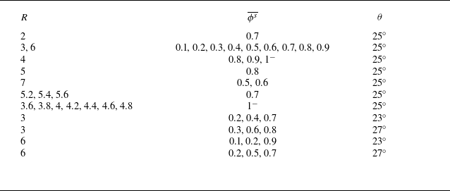


 Open access