

1. Introduction
1.1. Unsteady turbulent flow
Unsteady turbulent flow remains a topic of great interest in fluid mechanics due to its many intriguing characteristics that remain not fully understood as well as its broad practical applications in many engineering systems and natural environments, including, for example, the transient startup and shutdown of a power station, the closure or opening of a valve of a large water pipeline, sea waves over beaches, the blood flow in a vascular system and the unsteady flow in a turbo machine. Unsteady flows can be usefully classified into periodic and non-periodic flows, albeit similar underlying physics is often present in both cases. The present paper is concerned with the latter.
Maruyama, Kuribayashi & Mizushina (Reference Maruyama, Kuribayashi and Mizushina1976) carried out one of the earliest comprehensive experimental studies on turbulence responses following a step increase of flow rate from an initially turbulent flow. The experiments were conducted in a pipe of 51 mm diameter in a relatively low Reynolds number range of 5000–10 000. The axial velocity profiles were obtained using an electrochemical method, and through ensemble averaging based on repeated runs, both mean and turbulent fluctuating velocities were obtained. The authors identified that the generation and propagation of new turbulence are the dominant processes in a step-increase flow case, while the decay of the old turbulence is the dominant process in the step-decrease case. However, both cases are governed by the stepwise change of generation of turbulence corresponding to the final Reynolds number. Many years later, He & Jackson (Reference He and Jackson2000) performed an experimental study on linearly accelerating and decelerating flows, again from an initially turbulent flow. Differently from Maruyama et al.’s step-change case, the acceleration was maintained constant during the period of the experiments and the flow was varied in a much wider Reynolds number range of 7000–42 000. The measurements were conducted using a two-component laser Doppler anemometry (LDA), with which the three components of the velocity and turbulence were obtained by rotating the probe. The study confirmed the findings of Maruyama et al. that turbulence responds first in the wall region and propagates into the core. It further showed that the axial velocity responds earlier than that of the other components in the buffer region, but they all respond at approximately the same time in the core region. At any location, turbulence shows a two-stage response, namely an initial slow response followed by a rapid one. The overall transient turbulence behaviour was explained by associating it with turbulence production, energy redistribution between its components and propagation processes.
Greenblatt & Moss (Reference Greenblatt and Moss2004) conducted an experiment on an accelerating flow with much higher initial and final Reynolds numbers (31 000–82 000) and a much faster acceleration rate. Their results were generally supportive of the conclusions of the first two studies but, in addition, they observed a second peak turbulence response in a region further away from the wall at approximately
 $y^{+}=300$
. More recently, He, Ariyaratne & Vardy (Reference He, Ariyaratne and Vardy2011) conducted an experimental investigation on wall shear stress in an accelerating flow of water in a large-diameter pipe (100 mm) using flush-mount hot-film sensors. The response of the wall shear stress was found to undergo three-stage development which could be associated with the response of turbulence established in earlier studies. The first stage was related to a period where the turbulence response was minimum. The period of this stage was found to reduce with increase of the initial Reynolds number or increase of the acceleration. Chung (Reference Chung2005) conducted a direct numerical simulation (DNS) of transient channel flow following a sudden decrease in pressure gradient. The characteristics of the flow were found to be similar to those of a quasi-steady flow because the change of the pressure gradient was small. Seddighi et al. (Reference Seddighi, He, Orlandi and Vardy2011) carried out a similar DNS study but imposed a much stronger change in pressure gradient and also included a pressure step-up case. Turbulence becomes more anisotropic in both flows; there is more energy in the streamwise component than in the other two components in the step-up case, whereas the trend is reversed in the step-down case.
$y^{+}=300$
. More recently, He, Ariyaratne & Vardy (Reference He, Ariyaratne and Vardy2011) conducted an experimental investigation on wall shear stress in an accelerating flow of water in a large-diameter pipe (100 mm) using flush-mount hot-film sensors. The response of the wall shear stress was found to undergo three-stage development which could be associated with the response of turbulence established in earlier studies. The first stage was related to a period where the turbulence response was minimum. The period of this stage was found to reduce with increase of the initial Reynolds number or increase of the acceleration. Chung (Reference Chung2005) conducted a direct numerical simulation (DNS) of transient channel flow following a sudden decrease in pressure gradient. The characteristics of the flow were found to be similar to those of a quasi-steady flow because the change of the pressure gradient was small. Seddighi et al. (Reference Seddighi, He, Orlandi and Vardy2011) carried out a similar DNS study but imposed a much stronger change in pressure gradient and also included a pressure step-up case. Turbulence becomes more anisotropic in both flows; there is more energy in the streamwise component than in the other two components in the step-up case, whereas the trend is reversed in the step-down case.
In parallel, much research has also been carried out on accelerating flow from rest to study the effect of acceleration on laminar–turbulent transition. Kataoka, Kawabata & Miki (Reference Kataoka, Kawabata and Miki1975) studied the startup response to a step input of flow rate in a pipe using an electrochemical technique. They observed a systematic reduction of time before the occurrence of the laminar to turbulent transition with increase of the Reynolds number of the imposed flow. Kurokawa & Morikawa (Reference Kurokawa and Morikawa1986) conducted experiments on both accelerating and decelerating flows using hot-film probes and observed that even with a small acceleration, transition can be significantly delayed. They have noted two rather distinct transition patterns. The first is encountered when the acceleration is high, and at transition the mean velocity appears to decelerate near the wall but accelerate in the core. In contrast, when the acceleration is low, the trends in the core and wall are reversed. Moss (Reference Moss1989) also conducted experiments on accelerating flows from rest and found that the transitions they observed could be best associated with instabilities due to local flow conditions or those that originated from the turbulent structures carried downstream from the inlet of the pipe. Based on a series of experiments on constant acceleration from rest using water, Lefebvre & White (Reference Lefebvre and White1989) and Lefebvre & White (Reference Lefebvre and White1991) derived a simple relationship between the transitional Reynolds number and acceleration, which was further improved by Knisely, Nishihara & Iguchi (Reference Knisely, Nishihara and Iguchi2010) based on additional experiments with air. In addition, they have found that the transitional Reynolds number for flows starting from a laminar flow follows the same trend as those from rest and can also be well represented by the same expression. Annus & Koppel (Reference Annus and Koppel2011) studied transition from rest using a large-diameter pipe (
 $D=100~\text{mm}$
) with flush-mount hot-film sensors. Their results are consistent with transition observations in earlier studies based on smaller diameters. Following the approach of Koppel & Ainola (Reference Koppel and Ainola2006), they chose to correlate the dimensionless transitional (critical) time, rather than the Reynolds number, with the acceleration.
$D=100~\text{mm}$
) with flush-mount hot-film sensors. Their results are consistent with transition observations in earlier studies based on smaller diameters. Following the approach of Koppel & Ainola (Reference Koppel and Ainola2006), they chose to correlate the dimensionless transitional (critical) time, rather than the Reynolds number, with the acceleration.
Recently, based on DNS of a channel flow following a step increase of flow rate from an initially turbulent flow, the present authors proposed a new interpretation of the behaviours of the transient flow (He & Seddighi (Reference He and Seddighi2013); hereafter referred to as HS2013). Even though it started from a turbulent flow, the transient process was found to be effectively a laminar–turbulent transition. The transient process involves distinct phases of pre-transition, transition and full turbulence that are equivalent to the three regions of the boundary layer bypass transition, namely the buffeted laminar flow, the intermittent flow and the fully turbulent flow regions. In contrast to the spatial development, the initial response of the transient flow to the step increase of the flow rate is the formation of a thin layer of high strain rates on the wall, which grows into the core of the flow with time. The pre-existing turbulent structures act as perturbations to this boundary layer, much like the role that the free-stream turbulence plays in a bypass transition. These turbulent structures are modulated by the time-developing boundary layer and stretched to produce elongated streaks of high and low streamwise velocities, which remain stable in the pre-transitional period. However, later, in the transitional phase, they become unstable and localized turbulent spots are generated randomly in space. Such turbulent spots grow longitudinally as well as in the spanwise direction, merging with each other and eventually occupying the entire wall surface when the transition completes and the flow becomes fully turbulent. This transition concept is radically different from the theories that prevail in the unsteady flow literature. In essence, the traditional unsteady flow theories look at the evolution of turbulence following the perturbation of the mean flow, whereas the transition theory sees the new flow perturbation as the ‘base’ flow, studying its laminar-flow-natured development and then its transition to turbulence, while treating the pre-existing turbulent flow as disturbances. Nevertheless, as discussed in HS2013, the new theory explains well the observations of previous studies including, for example, Maruyama et al. (Reference Maruyama, Kuribayashi and Mizushina1976), He & Jackson (Reference He and Jackson2000), Greenblatt & Moss (Reference Greenblatt and Moss2004) and He et al. (Reference He, Ariyaratne and Vardy2011). In a follow-up study, Seddighi et al. (Reference Seddighi, He, Vardy and Orlandi2014) demonstrated that the transient response of a slowly accelerating flow shows a similar transitional behaviour.
In the study reported in HS2013, only one case was considered, where the initial and final Reynolds numbers (
 $\mathit{Re}=U_{b}{\it\delta}/{\it\nu}$
, where
$\mathit{Re}=U_{b}{\it\delta}/{\it\nu}$
, where
 $U_{b}$
is the bulk velocity of the flow
$U_{b}$
is the bulk velocity of the flow
 ${\it\delta}$
is the channel half-height and
${\it\delta}$
is the channel half-height and
 ${\it\nu}$
is the kinematic viscosity) were 2800 and 7400 respectively. An interesting question is how will the behaviour of the transient flow change when the initial and final Reynolds numbers are increased or decreased? In particular, what happens when the Reynolds number ratio is very small? Assuming that the flow rate is increased by only 20 %, for example, is the response of the flow still a distinct transition process? The purpose of this paper is to provide some answers to these questions by analysing results of DNS of a series of transient flows with systematically varied initial and final Reynolds numbers.
${\it\nu}$
is the kinematic viscosity) were 2800 and 7400 respectively. An interesting question is how will the behaviour of the transient flow change when the initial and final Reynolds numbers are increased or decreased? In particular, what happens when the Reynolds number ratio is very small? Assuming that the flow rate is increased by only 20 %, for example, is the response of the flow still a distinct transition process? The purpose of this paper is to provide some answers to these questions by analysing results of DNS of a series of transient flows with systematically varied initial and final Reynolds numbers.
Before proceeding to review the literature on bypass transition, it is useful to note that the above review is focused on non-periodic flows only. There are extensive studies of periodic flows around a non-zero mean, and oscillatory flows around zero mean flows. Readers interested in those topics are referred to recent studies of Scotti & Piomelli (Reference Scotti and Piomelli2001), Tardu & Da Costa (Reference Tardu and Da Costa2005), He & Jackson (Reference He and Jackson2009) and Manna, Vacca & Verzicco (Reference Manna, Vacca and Verzicco2012) for pulsating flows and Fornarelli & Vittori (Reference Fornarelli and Vittori2009) and Van der A et al. (Reference Van der A, O’Donoghue, Davies and Ribberink2011) for oscillatory flows.
1.2. Bypass transition
The theory of transition to turbulence is traditionally concerned with the natural transition where the two-dimensional Tollmien–Schlichting (TS) waves are amplified, leading to a three-dimensional secondary instability, which subsequently results in a breakdown of the flow to turbulence (referring to the review article Kachanov Reference Kachanov1994). The development of the TS waves is governed by the slow viscous process, and the transitional Reynolds number (
 $\mathit{Re}_{x,cr}$
) based on the free-stream velocity and the distance from the leading edge for a zero-pressure-gradient boundary is of the order of
$\mathit{Re}_{x,cr}$
) based on the free-stream velocity and the distance from the leading edge for a zero-pressure-gradient boundary is of the order of
 $10^{6}$
. However, this process can only be observed in boundary layers with small free-stream turbulence (FST). When the level of FST is
$10^{6}$
. However, this process can only be observed in boundary layers with small free-stream turbulence (FST). When the level of FST is
 ${>}1\,\%$
, the disturbances in the boundary layer develop rapidly and the breakdown occurs much earlier than that predicted by the traditional transition theory based on the TS instability. This scenario of transition is referred to as bypass transition, which typically occurs at a Reynolds number of the order of
${>}1\,\%$
, the disturbances in the boundary layer develop rapidly and the breakdown occurs much earlier than that predicted by the traditional transition theory based on the TS instability. This scenario of transition is referred to as bypass transition, which typically occurs at a Reynolds number of the order of
 $10^{5}$
or lower (see, for example, Klebanoff Reference Klebanoff1971; Boiko et al.
Reference Boiko, Westin, Klingmann, Kozlov and Alfredsson1994).
$10^{5}$
or lower (see, for example, Klebanoff Reference Klebanoff1971; Boiko et al.
Reference Boiko, Westin, Klingmann, Kozlov and Alfredsson1994).
Extensive studies have recently been carried out on the canonical bypass transition of a boundary layer over a flat plate subjected to FST. The free-stream turbulence enters the boundary layer either at the leading edge or through interactions with the boundary layer from above. The latter more readily allows disturbances of low frequencies to enter, whereas those of higher frequencies are filtered out; this is referred to as the sheltering effect (Hunt & Durbin Reference Hunt and Durbin1999; Hernon, Walsh & Mceligot Reference Hernon, Walsh and Mceligot2007; Zaki & Saha Reference Zaki and Saha2009). Often, unsteady streaky structures with high and low streamwise velocities develop and are enhanced downstream of the boundary layer, which is explained using the transient growth theory. Eventually, secondary instability develops and the boundary layer breaks down into turbulence. Much of this bypass transition process was demonstrated experimentally by Matsubara & Alfredsson (Reference Matsubara and Alfredsson2001) with detailed flow visualization as well as extensive hot-wire measurements in wind tunnels, and computationally by Jacobs & Durbin (Reference Jacobs and Durbin2001) using DNS. Matsubara & Alfredsson’s data demonstrated that the spanwise scale of the disturbances approaches the boundary layer thickness downstream after an initial adjustment, and that the energy of the streamwise velocity fluctuation grows linearly with downstream distance, which is consistent with observations in previous studies, e.g. Westin et al. (Reference Westin, Boiko, Klingmann, Kozlov and Alfredsson1994). The proportionality constants, however, vary from one experiment to another. Based on an extensive set of measurements of turbulence levels (
 $\mathit{Tu}$
) ranging from 1.4 to 6.7 %, Fransson, Matsubara & Alfredsson (Reference Fransson, Matsubara and Alfredsson2005) attempted to establish semi-empirical correlations for modelling the transition zone. They have shown that the initial disturbance energy in the boundary layer is proportional to
$\mathit{Tu}$
) ranging from 1.4 to 6.7 %, Fransson, Matsubara & Alfredsson (Reference Fransson, Matsubara and Alfredsson2005) attempted to establish semi-empirical correlations for modelling the transition zone. They have shown that the initial disturbance energy in the boundary layer is proportional to
 $\mathit{Tu}^{2}$
and that the transitional Reynolds number (
$\mathit{Tu}^{2}$
and that the transitional Reynolds number (
 $\mathit{Re}_{x,cr}$
) is proportional to
$\mathit{Re}_{x,cr}$
) is proportional to
 $\mathit{Tu}^{-2}$
. The authors also quantified the length of the transitional zone and found that it increases linearly with
$\mathit{Tu}^{-2}$
. The authors also quantified the length of the transitional zone and found that it increases linearly with
 $\mathit{Re}_{x,cr}$
.
$\mathit{Re}_{x,cr}$
.
The pre-transition energy growth was theoretically studied by Andersson, Berggren & Henningson (Reference Andersson, Berggren and Henningson1999) using optimal disturbance theory. The optimal disturbances consist of streamwise vortices developing into streamwise streaks, and the maximum energy growth was shown to be linearly proportional to the distance from the leading edge, hence reproducing experimental observations. This was also achieved independently by Luchini (Reference Luchini2000). Leib, Wundrow & Goldstein (Reference Leib, Wundrow and Goldstein1999)’s theoretical study was based on the solution of the boundary-region equation, which allowed them to more closely consider the interactions between the boundary layer and the free-stream disturbances. Their results showed that continuous free-stream forcing could play an important role in producing the large Klebanoff-mode growth rates observed in experiments, and that this growth exhibited a strong sensitivity to low-frequency anisotropy of the FST. Ricco (Reference Ricco2009) extended Leib et al.’s method to study the effects of convective-gust-type free-stream vortical disturbances on the Blasius boundary layer, which produced velocity profiles that compared well with experiments. Wundrow & Goldstein (Reference Wundrow and Goldstein2001) carried out an analysis based on the full nonlinear boundary-region equations. They demonstrated how an initially linear perturbation develops into nonlinear cross-flows. Such a flow could lead to a shear flow being locally highly inflectional, supporting the rapidly growing inviscid instabilities. They noted that the averaged streak amplitudes reported in experiments are likely to mask such strong localized distortions which can induce streak breakdown, causing discrepancies between theoretical predictions and experiments. This was verified recently by Nolan & Zaki (Reference Nolan and Zaki2013) using a DNS database.
Streak instability has been studied in searching for the mechanisms of breakdown to turbulence based on observations of flow structures (e.g. Brandt & Henningson Reference Brandt and Henningson2002; Zaki & Durbin Reference Zaki and Durbin2005; Schlatter et al. Reference Schlatter, Brandt, De Lange and Henningson2008; Mandal, Venkatakrishnan & Dey Reference Mandal, Venkatakrishnan and Dey2010; Nolan, Walsh & Mceligot Reference Nolan, Walsh and Mceligot2010; Nolan & Walsh Reference Nolan and Walsh2012). Additionally, Andersson et al. (Reference Andersson, Brandt, Bottaro and Henningson2001), Vaughan & Zaki (Reference Vaughan and Zaki2011) and Hack & Zaki (Reference Hack and Zaki2014) have performed secondary instability analysis of streaks. It is apparent that both the level and the scales of the FST can have a significant influence on when and how transition occurs. In their DNS study, Brandt, Schlatter & Henningson (Reference Brandt, Schlatter and Henningson2004) observed both sinuous and varicose breakdowns, although the former tends to occur more often and FST with larger length scales causes an earlier transition. Using a mixture of DNS and large-eddy simulation (LES), Nagarajan, Lele & Ferziger (Reference Nagarajan, Lele and Ferziger2007) found that both the bluntness of the leading edge and the FST level have an effect on the mechanisms of transition. For sharp edges with relatively low FST, transition usually occurs through instabilities on low-speed streaks, as observed by Jacobs & Durbin (Reference Jacobs and Durbin2001) and Brandt et al. (Reference Brandt, Schlatter and Henningson2004). For high FST or flow over a blunt leading edge, the transition was found to result from the amplification of the free-stream vortices at the leading edge due to stretching; these vortices grow as they convect downstream and eventually break down resulting in turbulent spots. These disturbances are wavepacket-like and occur in the lower part of the boundary layer. Ovchinnikov, Choudhari & Piomelli (Reference Ovchinnikov, Choudhari and Piomelli2008) observed that streamwise streaks have a clear dynamical significance only for a flow with small-length-scale FST. For a large-scale FST flow scenario, turbulent spots were formed upstream of the regions where streaks were detected. The spots’ precursors were short wavepackets in the wall-normal velocity components inside the boundary layer. Such wavepackets were noted to bear many differences from those observed by Nagarajan et al. (Reference Nagarajan, Lele and Ferziger2007), in which the wavepackets are in the spanwise velocity components and mostly stay in the lower part of the boundary layer. Based on the secondary instability analyses of a boundary layer distorted by both steady and unsteady Klebanoff streaks, Vaughan & Zaki (Reference Vaughan and Zaki2011) and Zaki (Reference Zaki2013) identified two most unstable modes, referred to as the inner and outer modes, which are apparently associated with the wavepacket- and streak-related transition mechanisms, respectively. Residing close to the wall, the inner mode is shielded from the high-frequency noise in the free stream and is believed to originate from the receptivity at the leading edge, consistent with the observations of Nagarajan et al. (Reference Nagarajan, Lele and Ferziger2007) and Ovchinnikov et al. (Reference Ovchinnikov, Choudhari and Piomelli2008). In the outer mode, the turbulence in the free stream provides an effective high-frequency forcing, causing an outer instability of the lifted streaks. This transition scenario was dominant, for example, in the DNS performed by Jacobs & Durbin (Reference Jacobs and Durbin2001).
The present study is concerned with the transition of a transient channel flow following a step increase of flow rate from an initially statistically steady turbulent flow. The initial and final Reynolds numbers of the transient flow are varied systematically, which results in scenarios with various FST structures and intensities (the latter is defined as the ratio of the root mean square (r.m.s.) of the turbulent fluctuating velocity of the initial flow to the final bulk velocity herein, which is discussed in § 3.2). This allows investigations into the effect of FST on the behaviours of transient flow transition and comparisons with results for the boundary layer transition discussed above.
The rest of the paper is structured as follows. After a description of the DNS numerical methods used in the present study in § 2, the results are presented and discussed in detail in § 3. The general picture of the transient flow is outlined in § 3.1 with the aid of flow visualizations, which is followed by an investigation into the effect of the initial and final Reynolds numbers on the timing of transition in § 3.2. Section 3.3 investigates the behaviour of the time-developing boundary layer, § 3.4 studies the energy growth during the pre-transition period and finally § 3.5 provides some quantifications of the flow structures. The paper is concluded with a summary of the key findings in § 4.
2. Numerical methods
DNS of transient turbulent channel flow is performed using an ‘in-house’ code solving the incompressible momentum and continuity equations:
 $$\begin{eqnarray}\displaystyle & \displaystyle \frac{\partial u_{i}^{\ast }}{\partial t^{\ast }}+u_{j}^{\ast }\frac{\partial u_{i}^{\ast }}{\partial x_{j}^{\ast }}=-\frac{\partial p^{\ast }}{\partial x_{i}^{\ast }}+\frac{1}{\mathit{Re}_{c}}{\rm\nabla}^{2}u_{i}^{\ast }, & \displaystyle\end{eqnarray}$$
 $$\begin{eqnarray}\displaystyle & \displaystyle \frac{\partial u_{i}^{\ast }}{\partial x_{i}^{\ast }}=0, & \displaystyle\end{eqnarray}$$
 $x_{1},x_{2},x_{3}$
and
$x_{1},x_{2},x_{3}$
and
 $u_{1},u_{2},u_{3}$
are the streamwise, wall-normal and spanwise coordinates and velocities respectively. The variables with an asterisk are non-dimensionalized using the density of the fluid (
$u_{1},u_{2},u_{3}$
are the streamwise, wall-normal and spanwise coordinates and velocities respectively. The variables with an asterisk are non-dimensionalized using the density of the fluid (
 ${\it\rho}$
), the channel half-height (
${\it\rho}$
), the channel half-height (
 ${\it\delta}$
) and the centreline velocity of the laminar Poiseuille flow at the initial flow rate (
${\it\delta}$
) and the centreline velocity of the laminar Poiseuille flow at the initial flow rate (
 $U_{c}$
). The Reynolds number is defined as
$U_{c}$
). The Reynolds number is defined as
 $\mathit{Re}_{c}=U_{c}{\it\delta}/{\it\nu}$
. However, unless otherwise stated, the time is rescaled using the bulk velocity of the final flow (
$\mathit{Re}_{c}=U_{c}{\it\delta}/{\it\nu}$
. However, unless otherwise stated, the time is rescaled using the bulk velocity of the final flow (
 $U_{b1}$
) as the characteristic velocity to facilitate direct comparison with data from literature, that is,
$U_{b1}$
) as the characteristic velocity to facilitate direct comparison with data from literature, that is,
 $t^{\ast }=tU_{b1}/{\it\delta}$
. The spatial derivatives of the governing equations are discretized using a second-order central finite difference method. For the temporal discretization, an explicit low-storage third-order Runge–Kutta scheme and a second-order implicit Crank–Nicholson scheme are used for the nonlinear and the viscous terms respectively. These are combined with the fractional-step method to enforce the continuity constraint (Kim & Moin Reference Kim and Moin1985; Orlandi Reference Orlandi2001). The Poisson equation is solved using fast Fourier transform (FFT). The code is parallelized using the message-passing interface (MPI) for use on a distributed-memory computer cluster. More details on the numerical methods used in the DNS code can be found in Seddighi (Reference Seddighi2011) or HS2013.
$t^{\ast }=tU_{b1}/{\it\delta}$
. The spatial derivatives of the governing equations are discretized using a second-order central finite difference method. For the temporal discretization, an explicit low-storage third-order Runge–Kutta scheme and a second-order implicit Crank–Nicholson scheme are used for the nonlinear and the viscous terms respectively. These are combined with the fractional-step method to enforce the continuity constraint (Kim & Moin Reference Kim and Moin1985; Orlandi Reference Orlandi2001). The Poisson equation is solved using fast Fourier transform (FFT). The code is parallelized using the message-passing interface (MPI) for use on a distributed-memory computer cluster. More details on the numerical methods used in the DNS code can be found in Seddighi (Reference Seddighi2011) or HS2013.
The channel flow is simulated using a computational domain with dimensions of
 $18({\it\delta}),2({\it\delta})$
and
$18({\it\delta}),2({\it\delta})$
and
 $5({\it\delta})$
for the streamwise, wall-normal and spanwise directions respectively. Periodic boundary conditions are used in the streamwise and spanwise directions, and no-slip boundary conditions are used for the top and bottom walls. The domain is meshed with a grid of
$5({\it\delta})$
for the streamwise, wall-normal and spanwise directions respectively. Periodic boundary conditions are used in the streamwise and spanwise directions, and no-slip boundary conditions are used for the top and bottom walls. The domain is meshed with a grid of
 $1024\times 240\times 480$
using a non-uniform distribution in the wall-normal direction and a uniform distribution along the other two directions. These can be compared with the domain
$1024\times 240\times 480$
using a non-uniform distribution in the wall-normal direction and a uniform distribution along the other two directions. These can be compared with the domain
 $12.8({\it\delta}),2({\it\delta})$
and
$12.8({\it\delta}),2({\it\delta})$
and
 $3.5({\it\delta})$
and mesh
$3.5({\it\delta})$
and mesh
 $512\times 190\times 200$
used in HS2013, which were carefully validated against previous benchmark data and checked for adequacy of the domain size using streamwise velocity correlations. A larger domain and mesh size are used in the present study to ensure that they are suitable for the whole range of Reynolds numbers used. The streamwise correlation of the streamwise velocity for each transient case was ensured to decay to approximately zero before the domain half-length. A summary of the non-dimensional grid sizes for the initial and final Reynolds numbers is shown in table 1 together with those used in HS2013 for direct comparison.
$512\times 190\times 200$
used in HS2013, which were carefully validated against previous benchmark data and checked for adequacy of the domain size using streamwise velocity correlations. A larger domain and mesh size are used in the present study to ensure that they are suitable for the whole range of Reynolds numbers used. The streamwise correlation of the streamwise velocity for each transient case was ensured to decay to approximately zero before the domain half-length. A summary of the non-dimensional grid sizes for the initial and final Reynolds numbers is shown in table 1 together with those used in HS2013 for direct comparison.
Mesh resolution in wall units at some typical Reynolds numbers.

A total of ten cases have been conducted, which are grouped into two series (table 2). In the first series (
 $\text{S}0X$
), the final Reynolds number (
$\text{S}0X$
), the final Reynolds number (
 $\mathit{Re}_{1}=U_{b1}{\it\delta}/{\it\nu}$
) is fixed at 7400, but the initial Reynolds number (
$\mathit{Re}_{1}=U_{b1}{\it\delta}/{\it\nu}$
) is fixed at 7400, but the initial Reynolds number (
 $\mathit{Re}_{0}=U_{b0}{\it\delta}/{\it\nu}$
) is varied from 2800 to 5300, where
$\mathit{Re}_{0}=U_{b0}{\it\delta}/{\it\nu}$
) is varied from 2800 to 5300, where
 $U_{b0}$
and
$U_{b0}$
and
 $U_{b1}$
are the bulk velocities of the initial and final flows respectively. In the second series (
$U_{b1}$
are the bulk velocities of the initial and final flows respectively. In the second series (
 $\text{S}1X$
),
$\text{S}1X$
),
 $\mathit{Re}_{0}$
is fixed at 2800 but
$\mathit{Re}_{0}$
is fixed at 2800 but
 $\mathit{Re}_{1}$
is varied from 3100 to 12 600. Case S01 is the same as that of HS2013. For the smallest increase of flow rate, the Reynolds number is increased by only
$\mathit{Re}_{1}$
is varied from 3100 to 12 600. Case S01 is the same as that of HS2013. For the smallest increase of flow rate, the Reynolds number is increased by only
 ${\sim}10\,\%$
(S16), whereas the increase is 450 % in S11. For each case, at least five runs were carried out to facilitate the calculations of flow statistics using ensemble averaging. To generate independent initial flow fields, simulation at a constant mass flow corresponding to the initial Reynolds number of any case in table 2 is carried out until it has reached a stationary state, after which it is run for a further period of time, so independent flow fields with long time intervals between them are saved. Each transient flow is started from one such flow field, being accelerated rapidly and linearly to the final Reynolds number, after which it is run at a constant mass flow for a sufficiently long time for the flow to become fully developed (statistically steady) again. The acceleration is so rapid that the flow can be seen as undergoing a step increase. The non-dimensional ramp period (
${\sim}10\,\%$
(S16), whereas the increase is 450 % in S11. For each case, at least five runs were carried out to facilitate the calculations of flow statistics using ensemble averaging. To generate independent initial flow fields, simulation at a constant mass flow corresponding to the initial Reynolds number of any case in table 2 is carried out until it has reached a stationary state, after which it is run for a further period of time, so independent flow fields with long time intervals between them are saved. Each transient flow is started from one such flow field, being accelerated rapidly and linearly to the final Reynolds number, after which it is run at a constant mass flow for a sufficiently long time for the flow to become fully developed (statistically steady) again. The acceleration is so rapid that the flow can be seen as undergoing a step increase. The non-dimensional ramp period (
 ${\rm\Delta}t^{\ast }$
) is between 0.006 and 0.36, but the period during which the flow exhibits transient behaviour is approximately
${\rm\Delta}t^{\ast }$
) is between 0.006 and 0.36, but the period during which the flow exhibits transient behaviour is approximately
 $t^{\ast }=50{-}80$
, where
$t^{\ast }=50{-}80$
, where
 $t^{\ast }=tU_{b1}/{\it\delta}$
. We have adopted a constant mass flow approach (as opposed to a constant pressure gradient approach) in the simulations presented herein. To initiate the acceleration, an additional source term is added to the streamwise ‘mean’ pressure gradient at
$t^{\ast }=tU_{b1}/{\it\delta}$
. We have adopted a constant mass flow approach (as opposed to a constant pressure gradient approach) in the simulations presented herein. To initiate the acceleration, an additional source term is added to the streamwise ‘mean’ pressure gradient at
 $t^{\ast }=0$
, the detail of which can be found in Seddighi (Reference Seddighi2011) or HS2013.
$t^{\ast }=0$
, the detail of which can be found in Seddighi (Reference Seddighi2011) or HS2013.
The unsteady flow cases studied.

The ensemble averaged statistical quantities for any location at a distance of
 $y_{1}$
from the wall are obtained through averaging over the plane of
$y_{1}$
from the wall are obtained through averaging over the plane of
 $y=y_{1}$
as well as using the repeated runs. Thus, the local mean velocity is
$y=y_{1}$
as well as using the repeated runs. Thus, the local mean velocity is
 $$\begin{eqnarray}\overline{u}_{s}=\frac{1}{MNL}\left(\mathop{\sum }_{k=1}^{L}\mathop{\sum }_{j=1}^{N}\mathop{\sum }_{i=1}^{M}u_{s}\right),\end{eqnarray}$$
and the r.m.s. of the turbulent fluctuating velocity is
 $$\begin{eqnarray}u_{s,rms}^{\prime }=\sqrt{\frac{1}{MNL}\left(\mathop{\sum }_{k=1}^{L}\mathop{\sum }_{j=1}^{N}\mathop{\sum }_{i=1}^{M}(u_{s}-\overline{u}_{s})^{2}\right)},\end{eqnarray}$$
where
 $M$
and
$M$
and
 $N$
are the numbers of data points in the streamwise and spanwise directions respectively,
$N$
are the numbers of data points in the streamwise and spanwise directions respectively,
 $L$
is the number of repeated runs and
$L$
is the number of repeated runs and
 $s=1,2,3$
for the streamwise, wall-normal and spanwise velocities, which are also denoted as
$s=1,2,3$
for the streamwise, wall-normal and spanwise velocities, which are also denoted as
 $u$
,
$u$
,
 $v$
and
$v$
and
 $w$
. The results for the top and bottom half-channels are found to be practically identical, which serves as an indication of the convergence of the statistical calculations. The results presented in this paper are averaged over the top and bottom half-channels where appropriate.
$w$
. The results for the top and bottom half-channels are found to be practically identical, which serves as an indication of the convergence of the statistical calculations. The results presented in this paper are averaged over the top and bottom half-channels where appropriate.
3. Results and discussion
3.1. The general picture
The flow structures at several instants during the transient period in selected cases are shown in figure 1 using three-dimensional isosurface plots of
 $u^{\prime }/U_{b0}$
and
$u^{\prime }/U_{b0}$
and
 ${\it\lambda}_{2}/(U_{b0}/{\it\delta})^{2}$
. Here,
${\it\lambda}_{2}/(U_{b0}/{\it\delta})^{2}$
. Here,
 $u^{\prime }(=u-\bar{u})$
is the instantaneous streamwise fluctuating velocity and
$u^{\prime }(=u-\bar{u})$
is the instantaneous streamwise fluctuating velocity and
 ${\it\lambda}_{2}$
is the second largest eigenvalue of the symmetric tensor
${\it\lambda}_{2}$
is the second largest eigenvalue of the symmetric tensor
 $\unicode[STIX]{x1D64E}^{2}+{\it\bf\Omega}^{2}$
, where
$\unicode[STIX]{x1D64E}^{2}+{\it\bf\Omega}^{2}$
, where
 $\unicode[STIX]{x1D64E}$
and
$\unicode[STIX]{x1D64E}$
and
 ${\it\bf\Omega}$
are the symmetric and antisymmetric parts of the velocity gradient tensor
${\it\bf\Omega}$
are the symmetric and antisymmetric parts of the velocity gradient tensor
 $\boldsymbol{{\rm\nabla}}\boldsymbol{u}$
. This was initially proposed by Jeong & Hussain (Reference Jeong and Hussain1995) as an effective indicator for vortical structures and has since been used in the study of turbulence and transition. All the cases shown in the figure have the same initial Reynolds number (
$\boldsymbol{{\rm\nabla}}\boldsymbol{u}$
. This was initially proposed by Jeong & Hussain (Reference Jeong and Hussain1995) as an effective indicator for vortical structures and has since been used in the study of turbulence and transition. All the cases shown in the figure have the same initial Reynolds number (
 $\mathit{Re}_{0}=2800$
) but very different final Reynolds numbers, namely 12 600, 5000 and 3100 for S11, S13 and S16 respectively. These can be compared with the flow studied in HS2013 in which
$\mathit{Re}_{0}=2800$
) but very different final Reynolds numbers, namely 12 600, 5000 and 3100 for S11, S13 and S16 respectively. These can be compared with the flow studied in HS2013 in which
 $\mathit{Re}$
was varied between 2800 and 7400.
$\mathit{Re}$
was varied between 2800 and 7400.
Streaks and vortex structures in three-dimensional plots of isosurfaces in (a) S11, (b) S13 and (c) S16. Streaks are shown in green/blue with
 $u^{\prime }/U_{b0}=\pm 0.35$
and vortical structures are shown in red with
$u^{\prime }/U_{b0}=\pm 0.35$
and vortical structures are shown in red with
 ${\it\lambda}_{2}/(U_{bo}/{\it\delta})^{2}=-5$
.
${\it\lambda}_{2}/(U_{bo}/{\it\delta})^{2}=-5$
.

We first consider the flow with the highest change of flow rate, i.e. case S11. In the initial flow (
 $t^{\ast }=0$
), patches of fluids with high or low fluctuating velocities are clearly in existence and some hairpin structures are also identifiable through the isosurfaces of
$t^{\ast }=0$
), patches of fluids with high or low fluctuating velocities are clearly in existence and some hairpin structures are also identifiable through the isosurfaces of
 ${\it\lambda}_{2}$
. These are rather uniformly distributed in the flow field, showing the picture of a typical turbulent shear flow. During the early period (appropriately,
${\it\lambda}_{2}$
. These are rather uniformly distributed in the flow field, showing the picture of a typical turbulent shear flow. During the early period (appropriately,
 $t^{\ast }<29$
), elongated streaks are formed, as evident by the long tubes of isosurfaces of positive and negative
$t^{\ast }<29$
), elongated streaks are formed, as evident by the long tubes of isosurfaces of positive and negative
 $u^{\prime }/U_{b0}$
which appear alternately to each other. Such flow structures are common and representative in the pre-transition and transition regions of boundary layers (e.g. Jacobs & Durbin Reference Jacobs and Durbin2001; Matsubara & Alfredsson Reference Matsubara and Alfredsson2001). The number of hairpins appears to reduce during the early stage of this period, but new vortical structures start to appear in clusters at approximately
$u^{\prime }/U_{b0}$
which appear alternately to each other. Such flow structures are common and representative in the pre-transition and transition regions of boundary layers (e.g. Jacobs & Durbin Reference Jacobs and Durbin2001; Matsubara & Alfredsson Reference Matsubara and Alfredsson2001). The number of hairpins appears to reduce during the early stage of this period, but new vortical structures start to appear in clusters at approximately
 $t^{\ast }=29$
, which indicates the generation of turbulent spots, signifying the onset of transition. During the period to follow (approximately,
$t^{\ast }=29$
, which indicates the generation of turbulent spots, signifying the onset of transition. During the period to follow (approximately,
 $29<t^{\ast }<55$
), such turbulent spots grow to occupy more spaces, joining with each other, and eventually at approximately
$29<t^{\ast }<55$
), such turbulent spots grow to occupy more spaces, joining with each other, and eventually at approximately
 $t^{\ast }\sim 55$
, the entire surface is covered with newly generated turbulence. The isosurface tubes (streaks) break up along with the generation of turbulent spots as the transition progresses. The vortices often occur around the low-speed streaks accompanying their breakup in this case, which is again similar to those shown in boundary layer bypass transition (e.g. Jacobs & Durbin Reference Jacobs and Durbin2001; Schlatter et al.
Reference Schlatter, Brandt, De Lange and Henningson2008). The basic features of the flow described above are similar to those found in HS2013, although the streaks during the pre-transition and transition periods are stronger and more striking in S11.
$t^{\ast }\sim 55$
, the entire surface is covered with newly generated turbulence. The isosurface tubes (streaks) break up along with the generation of turbulent spots as the transition progresses. The vortices often occur around the low-speed streaks accompanying their breakup in this case, which is again similar to those shown in boundary layer bypass transition (e.g. Jacobs & Durbin Reference Jacobs and Durbin2001; Schlatter et al.
Reference Schlatter, Brandt, De Lange and Henningson2008). The basic features of the flow described above are similar to those found in HS2013, although the streaks during the pre-transition and transition periods are stronger and more striking in S11.
Development of the friction coefficient with equivalent Reynolds number (
 $\mathit{Re}_{t}=tU_{b1}^{2}/{\it\nu}$
): (a) effect of varying
$\mathit{Re}_{t}=tU_{b1}^{2}/{\it\nu}$
): (a) effect of varying
 $\mathit{Re}_{0}$
(same
$\mathit{Re}_{0}$
(same
 $\mathit{Re}_{1}$
); (b) effect of varying
$\mathit{Re}_{1}$
); (b) effect of varying
 $\mathit{Re}_{1}$
(same
$\mathit{Re}_{1}$
(same
 $\mathit{Re}_{0}$
).
$\mathit{Re}_{0}$
).

Overall, case S13 (which has a ‘medium’ Reynolds number ratio) follows a similar trend (figure 1 b), but the strength of the streaks is much weaker and the generation of turbulent spots seems to occur at a lower rate and the changes are less striking. This trend is similar to the transition of a boundary layer subject to a higher level of FST. For example, in a boundary layer subject to a 7 % FST, Jacobs & Durbin (Reference Jacobs and Durbin2001) found that although streaks and jets are present in such flows, they are surrounded by elevated turbulence and distinct turbulent spots are much more difficult to discern. In the case of S16 where the Reynolds number was only increased by 10 %, the flow structures appear to be characteristically different (figure 1 c). It is clear that the turbulent activities at the end of the transient are stronger than those at the beginning, but the distinct transition is not seen. There are no clear signs of generation of elongated streaks at the pre-transition stage nor obvious enhancement of the generation of turbulent spots during the transition period.
The above results show that the phenomenological features of transition of the transient flow identified in HS2013 are strong and well pronounced when the difference between the final and initial Reynolds numbers is high, but less pronounced, though still clearly in existence, when it is reduced. When the Reynolds number difference is very low, however, the transitional process is difficult to identify from the visualization presented above.
In the rest of the paper, various statistics of the mean flow and turbulence are analysed to quantify the flow structures observed above to establish the effect of varying the initial and final Reynolds numbers. It will become clear that although the visualization of the flow structures shows that the transient process of lower-Reynolds-number-ratio cases appears to be qualitatively different, they in fact show as much a transition characteristic as the higher-Reynolds-number-ratio cases in the parameters used to identify such processes, and the critical equivalent Reynolds number (defined later) in all the flows studied can be correlated using a simple expression.
3.2. Effect of initial and final Reynolds numbers
The variations of the friction coefficient (
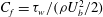 $C_{f}={\it\tau}_{w}/({\it\rho}U_{b}^{2}/2)$
, where
$C_{f}={\it\tau}_{w}/({\it\rho}U_{b}^{2}/2)$
, where
 ${\it\tau}_{w}$
is the wall shear stress) in the various cases investigated in this study are inspected to establish the overall behaviour of the flow response (figure 2). Here, we use an alternative non-dimensional time to
${\it\tau}_{w}$
is the wall shear stress) in the various cases investigated in this study are inspected to establish the overall behaviour of the flow response (figure 2). Here, we use an alternative non-dimensional time to
 $t^{\ast }$
, namely
$t^{\ast }$
, namely
 $$\begin{eqnarray}\mathit{Re}_{t}=\frac{tU_{b1}^{2}}{{\it\nu}},\end{eqnarray}$$
which is referred to as the equivalent Reynolds number herein. Considering the bulk velocity
 $U_{b1}$
as a characteristic convective velocity, together with the time
$U_{b1}$
as a characteristic convective velocity, together with the time
 $t$
, it defines a length
$t$
, it defines a length
 $x=U_{b1}t$
, representing the distance that a fluid particle has travelled after the commencement of the transient. As a result, the equivalent Reynolds number can be written as
$x=U_{b1}t$
, representing the distance that a fluid particle has travelled after the commencement of the transient. As a result, the equivalent Reynolds number can be written as
 $\mathit{Re}_{t}=(xU_{b1})/{\it\nu}$
, mirroring the Reynolds number
$\mathit{Re}_{t}=(xU_{b1})/{\it\nu}$
, mirroring the Reynolds number
 $\mathit{Re}_{x}$
used in the boundary layer based on the free-stream velocity and the distance from the leading edge. It will be demonstrated later that
$\mathit{Re}_{x}$
used in the boundary layer based on the free-stream velocity and the distance from the leading edge. It will be demonstrated later that
 $\mathit{Re}_{t}$
indeed has the same significance in a transient flow transition as
$\mathit{Re}_{t}$
indeed has the same significance in a transient flow transition as
 $\mathit{Re}_{x}$
in the boundary layer transition, although direct quantitative comparison between the two quantities is not appropriate. It is useful to note that
$\mathit{Re}_{x}$
in the boundary layer transition, although direct quantitative comparison between the two quantities is not appropriate. It is useful to note that
 $\mathit{Re}_{t}=t^{\ast }\mathit{Re}_{1}$
, where
$\mathit{Re}_{t}=t^{\ast }\mathit{Re}_{1}$
, where
 $t^{\ast }=tU_{b1}/{\it\delta}$
and
$t^{\ast }=tU_{b1}/{\it\delta}$
and
 $\mathit{Re}_{1}=U_{b1}{\it\delta}/{\it\nu}$
.
$\mathit{Re}_{1}=U_{b1}{\it\delta}/{\it\nu}$
.
Focusing on case S11 first, it can be seen that the
 $C_{f}$
reaches a very high value (off scale) immediately after the commencement of the excursion due to the inertia resulting from the rapid flow acceleration in a very short period of time. From there, it decreases monotonically until approximately
$C_{f}$
reaches a very high value (off scale) immediately after the commencement of the excursion due to the inertia resulting from the rapid flow acceleration in a very short period of time. From there, it decreases monotonically until approximately
 $\mathit{Re}_{t}=3.6\times 10^{5}$
(or,
$\mathit{Re}_{t}=3.6\times 10^{5}$
(or,
 $t^{\ast }=29$
) where it reaches a minimum, after which it increases again to approximately the final steady value at
$t^{\ast }=29$
) where it reaches a minimum, after which it increases again to approximately the final steady value at
 $\mathit{Re}_{t}=7.0\times 10^{5}$
, or
$\mathit{Re}_{t}=7.0\times 10^{5}$
, or
 $t^{\ast }=55$
. Comparing with the flow visualization of the corresponding case (figure 1
a), it is clear that the timing of the minimum
$t^{\ast }=55$
. Comparing with the flow visualization of the corresponding case (figure 1
a), it is clear that the timing of the minimum
 $C_{f}$
roughly coincides with the initial stage of the generation of turbulence spots. Following HS2013, we refer to the time when
$C_{f}$
roughly coincides with the initial stage of the generation of turbulence spots. Following HS2013, we refer to the time when
 $C_{f}$
reaches the minimum as the point of the ‘onset of transition’ and the corresponding non-dimensional time as the critical equivalent Reynolds number
$C_{f}$
reaches the minimum as the point of the ‘onset of transition’ and the corresponding non-dimensional time as the critical equivalent Reynolds number
 $\mathit{Re}_{t,cr}$
or, equivalently, the critical time
$\mathit{Re}_{t,cr}$
or, equivalently, the critical time
 $t_{cr}^{\ast }$
.
$t_{cr}^{\ast }$
.
The effect of varying the initial and final Reynolds numbers (
 $\mathit{Re}_{0}$
and
$\mathit{Re}_{0}$
and
 $\mathit{Re}_{1}$
) on the overall flow behaviour is now studied by comparing the responses of
$\mathit{Re}_{1}$
) on the overall flow behaviour is now studied by comparing the responses of
 $C_{f}$
in the various cases. Figure 2(a) shows that
$C_{f}$
in the various cases. Figure 2(a) shows that
 $\mathit{Re}_{t,cr}$
reduces monotonically with increase of
$\mathit{Re}_{t,cr}$
reduces monotonically with increase of
 $\mathit{Re}_{0}$
. For a fixed
$\mathit{Re}_{0}$
. For a fixed
 $\mathit{Re}_{1}$
of 7400,
$\mathit{Re}_{1}$
of 7400,
 $\mathit{Re}_{t,cr}$
reduces from
$\mathit{Re}_{t,cr}$
reduces from
 $1.47\times 10^{5}$
to
$1.47\times 10^{5}$
to
 $5.50\times 10^{4}$
when
$5.50\times 10^{4}$
when
 $\mathit{Re}_{0}$
is increased from 2800 to 5300. In addition, alongside the reduction of
$\mathit{Re}_{0}$
is increased from 2800 to 5300. In addition, alongside the reduction of
 $\mathit{Re}_{t,cr}$
, the minimum friction coefficient increases significantly, showing a progressively smaller ‘undershooting’ of the final
$\mathit{Re}_{t,cr}$
, the minimum friction coefficient increases significantly, showing a progressively smaller ‘undershooting’ of the final
 $C_{f}$
. Figure 2(b) shows that increasing
$C_{f}$
. Figure 2(b) shows that increasing
 $\mathit{Re}_{1}$
results in an increase in
$\mathit{Re}_{1}$
results in an increase in
 $\mathit{Re}_{t,cr}$
. For a fixed
$\mathit{Re}_{t,cr}$
. For a fixed
 $\mathit{Re}_{0}$
of 2800, as
$\mathit{Re}_{0}$
of 2800, as
 $\mathit{Re}_{1}$
is increased from 3100 to 12 600,
$\mathit{Re}_{1}$
is increased from 3100 to 12 600,
 $\mathit{Re}_{t,cr}$
increases from
$\mathit{Re}_{t,cr}$
increases from
 $3.30\times 10^{4}$
to
$3.30\times 10^{4}$
to
 $3.65\times 10^{5}$
. In addition, the minimum
$3.65\times 10^{5}$
. In addition, the minimum
 $C_{f}$
varies from a very small ‘undershooting’ at
$C_{f}$
varies from a very small ‘undershooting’ at
 $\mathit{Re}_{1}=3100$
to a strong one at
$\mathit{Re}_{1}=3100$
to a strong one at
 $\mathit{Re}_{1}=12\,600$
. The final
$\mathit{Re}_{1}=12\,600$
. The final
 $C_{f}$
reduces with increase of
$C_{f}$
reduces with increase of
 $\mathit{Re}_{1}$
. It is of most interest that the friction factor in all cases, including those with a very small
$\mathit{Re}_{1}$
. It is of most interest that the friction factor in all cases, including those with a very small
 $\mathit{Re}$
ratio, shows the same characteristic behaviour even though
$\mathit{Re}$
ratio, shows the same characteristic behaviour even though
 $\mathit{Re}_{t,cr}$
and the level of undershooting of
$\mathit{Re}_{t,cr}$
and the level of undershooting of
 $C_{f}$
can be very different in the different cases. It will be shown later that the flow before the critical point always behaves like a laminar flow despite the significant differences in the initial Reynolds number and the level of flow perturbation. Overall, the critical time
$C_{f}$
can be very different in the different cases. It will be shown later that the flow before the critical point always behaves like a laminar flow despite the significant differences in the initial Reynolds number and the level of flow perturbation. Overall, the critical time
 $t_{cr}^{\ast }$
shows a similar trend to that of the equivalent Reynolds number
$t_{cr}^{\ast }$
shows a similar trend to that of the equivalent Reynolds number
 $\mathit{Re}_{t,cr}$
described above, reducing with increase of the initial Reynolds number or decrease of the final Reynolds number.
$\mathit{Re}_{t,cr}$
described above, reducing with increase of the initial Reynolds number or decrease of the final Reynolds number.
The mechanisms by which the initial and final Reynolds numbers affect the transition process and the critical equivalent Reynolds number are no doubt very complex. It has been well established in boundary layer research that the transition is strongly influenced by the level of FST, referring to Andersson et al. (Reference Andersson, Berggren and Henningson1999), Luchini (Reference Luchini2000), Brandt et al. (Reference Brandt, Schlatter and Henningson2004), Fransson et al. (Reference Fransson, Matsubara and Alfredsson2005), Nagarajan et al. (Reference Nagarajan, Lele and Ferziger2007) and Ovchinnikov et al. (Reference Ovchinnikov, Choudhari and Piomelli2008). Moreover, Brandt et al. (Reference Brandt, Schlatter and Henningson2004) and Ovchinnikov et al. (Reference Ovchinnikov, Choudhari and Piomelli2008) also showed that both the critical Reynolds number and also possibly the mechanisms of transition are affected by the length scales of the FST. In light of such understanding, the following factors are candidates for consideration, which can potentially influence the behaviours of the transient process when the Reynolds numbers are varied.
-
(i)
 $\mathit{Re}_{0}$
(
$=U_{b0}{\it\delta}/{\it\nu}$
), which defines the initial turbulence in terms of the amplitude and time/length scales. The higher
$\mathit{Re}_{0}$
is, the lower the initial turbulence intensity is but also the smaller the time/length scales are. It also defines the initial mean velocity profile.
$\mathit{Re}_{0}$
(
$=U_{b0}{\it\delta}/{\it\nu}$
), which defines the initial turbulence in terms of the amplitude and time/length scales. The higher
$\mathit{Re}_{0}$
is, the lower the initial turbulence intensity is but also the smaller the time/length scales are. It also defines the initial mean velocity profile. -
(ii)
$\mathit{Re}_{1}$
, which defines the ‘free-stream’ velocity. Arguably this is the most important velocity of the transient flow. -
(iii)
$(\mathit{Re}_{1}-\mathit{Re}_{0})$
, which defines
$(U_{b1}-U_{b0})$
, is the cause of the change. Indeed, the time-developing boundary layer is characterized by this velocity (see § 3.3). -
(iv) The acceleration rate,
$(U_{b1}-U_{b0})/{\rm\Delta}t$
. This could potentially be a factor. However, in all cases considered herein, the acceleration is very rapid and the flow increase can be viewed as a step change. Tests with the acceleration rate increased by an order of magnitude show no effect on the transition behaviour. For a transient with a much slower rate, the acceleration rates does affect the
$\mathit{Re}_{t,cr}$
but the general transition process remains similar (Seddighi et al.
Reference Seddighi, He, Vardy and Orlandi2014). -
(v) The initial FST intensity (
$\mathit{Tu}_{0}$
). This is dependent on both
$\mathit{Re}_{0}$
and
$\mathit{Re}_{1}$
, which can be represented by
$(u_{rms,0}^{\prime })_{max}/U_{b1}$
, as explained later, where
$(u_{rms,0}^{\prime })_{max}$
is the peak value of the wall-normal profile of the r.m.s. of the streamwise turbulent fluctuating velocity at
$t=0$
.


We have investigated the various mechanisms discussed above and correlated the data against alternative parameters. It has become evident that, as far as the critical Reynolds number is concerned, the dominant effect of varying
 $\mathit{Re}_{0}$
and
$\mathit{Re}_{0}$
and
 $\mathit{Re}_{1}$
is through changing the initial FST intensity, as demonstrated below.
$\mathit{Re}_{1}$
is through changing the initial FST intensity, as demonstrated below.
First, let us derive a way of describing the initial turbulent intensity, that is, the equivalent FST. We consider a very early instant of the transient flow following the step increase of the flow rate. At this stage, the turbulence remains unchanged from that of the initial flow and the mean velocity is that of the final flow. The turbulence in a fully developed channel is very different from the FST of the boundary layer, being highly anisotropic and non-uniform normal to the wall. For simplicity and unambiguity, we choose the peak value of the wall-normal profile to represent the turbulence level. Consequently the initial free-stream turbulence intensity can be written as
 $$\begin{eqnarray}\mathit{Tu}_{0}=\frac{\left(u_{rms,0}^{\prime }\right)_{\!max}}{U_{b1}}=\left(\frac{U_{b0}}{U_{b1}}\right)\frac{\left(u_{rms,0}^{\prime }\right)_{max}}{U_{b0}}.\end{eqnarray}$$
The ratio
 $(u_{rms,0}^{\prime })_{max}/U_{b0}$
is the peak turbulence intensity of the initial flow before the commencement of the transient. Recently, there has been considerable interest in the effect of the Reynolds number on the peak turbulence intensity in wall units, i.e.
$(u_{rms,0}^{\prime })_{max}/U_{b0}$
is the peak turbulence intensity of the initial flow before the commencement of the transient. Recently, there has been considerable interest in the effect of the Reynolds number on the peak turbulence intensity in wall units, i.e.
 $(u_{rms}^{\prime +})_{max}=(u_{rms}^{\prime })_{max}/u_{{\it\tau}}$
(Hultmark, Bailey & Smits Reference Hultmark, Bailey and Smits2010; Ng et al.
Reference Ng, Monty, Hutchins, Chong and Marusic2011; Hultmark et al.
Reference Hultmark, Vallikivi, Bailey and Smits2013). It has been established that
$(u_{rms}^{\prime +})_{max}=(u_{rms}^{\prime })_{max}/u_{{\it\tau}}$
(Hultmark, Bailey & Smits Reference Hultmark, Bailey and Smits2010; Ng et al.
Reference Ng, Monty, Hutchins, Chong and Marusic2011; Hultmark et al.
Reference Hultmark, Vallikivi, Bailey and Smits2013). It has been established that
 $(u_{rms}^{\prime +})_{max}$
varies with the Reynolds number in a boundary layer and a channel flow, whereas there are still some dispute on whether
$(u_{rms}^{\prime +})_{max}$
varies with the Reynolds number in a boundary layer and a channel flow, whereas there are still some dispute on whether
 $(u_{rms}^{\prime +})_{max}$
is also dependent on the Reynolds number for pipe flows. In any case, it is well established that the turbulence intensity expressed in the outer scaling,
$(u_{rms}^{\prime +})_{max}$
is also dependent on the Reynolds number for pipe flows. In any case, it is well established that the turbulence intensity expressed in the outer scaling,
 $(u_{rms}^{\prime })_{max}/U_{b}$
, is a function of the Reynolds number. The present DNS data for
$(u_{rms}^{\prime })_{max}/U_{b}$
, is a function of the Reynolds number. The present DNS data for
 $2800<\mathit{Re}<12\,600$
show that
$2800<\mathit{Re}<12\,600$
show that
 $(u_{rms}^{\prime })_{max}/U_{b}\sim \mathit{Re}^{-0.1}$
, and hence the free-stream turbulence (
$(u_{rms}^{\prime })_{max}/U_{b}\sim \mathit{Re}^{-0.1}$
, and hence the free-stream turbulence (
 $\mathit{Tu}_{0}$
) defined in (3.2) is proportional to
$\mathit{Tu}_{0}$
) defined in (3.2) is proportional to
 $(U_{b0}/U_{b1})\mathit{Re}_{0}^{-0.1}$
. In fact, the following expression represents the DNS
$(U_{b0}/U_{b1})\mathit{Re}_{0}^{-0.1}$
. In fact, the following expression represents the DNS
 $\mathit{Tu}_{0}$
extremely closely:
$\mathit{Tu}_{0}$
extremely closely:
 $$\begin{eqnarray}\mathit{Tu}_{0}=0.375\left(\frac{U_{b0}}{U_{b1}}\right)\left(\mathit{Re}_{0}\right)^{-0.1}.\end{eqnarray}$$
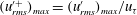
Dependence of the critical equivalent Reynolds number on the velocity ratio.

Dependence of the critical equivalent Reynolds number on the initial FST intensity.

Figure 3 shows the critical equivalent Reynolds number (
 $\mathit{Re}_{t,cr}$
) plotted against the velocity ratio (equivalent to the Reynolds number ratio) in double logarithmic scale. The data correlate reasonably well, which suggests a strong dependence of
$\mathit{Re}_{t,cr}$
) plotted against the velocity ratio (equivalent to the Reynolds number ratio) in double logarithmic scale. The data correlate reasonably well, which suggests a strong dependence of
 $\mathit{Re}_{t,cr}$
on the velocity ratio. In fact, all the data of the
$\mathit{Re}_{t,cr}$
on the velocity ratio. In fact, all the data of the
 $\text{S}1X$
series (with the same
$\text{S}1X$
series (with the same
 $\mathit{Re}_{0}$
but different
$\mathit{Re}_{0}$
but different
 $\mathit{Re}_{1}$
) lie nearly perfectly on a straight line, implying that
$\mathit{Re}_{1}$
) lie nearly perfectly on a straight line, implying that
 $\mathit{Re}_{t,cr}$
and
$\mathit{Re}_{t,cr}$
and
 $U_{b0}/U_{b1}$
are related in a power-law form. On the other hand, all of the data of series
$U_{b0}/U_{b1}$
are related in a power-law form. On the other hand, all of the data of series
 $\text{S}0X$
(with fixed
$\text{S}0X$
(with fixed
 $\mathit{Re}_{1}$
but varying
$\mathit{Re}_{1}$
but varying
 $\mathit{Re}_{0}$
) appear also to lie on a straight line, which suggests a systematic
$\mathit{Re}_{0}$
) appear also to lie on a straight line, which suggests a systematic
 $\mathit{Re}_{0}$
effect. By trial and error, it has been established that the effect of varying the initial Reynolds number is closely represented by
$\mathit{Re}_{0}$
effect. By trial and error, it has been established that the effect of varying the initial Reynolds number is closely represented by
 $\mathit{Re}_{0}^{-0.1}$
, and the two series of data are brought closely together when
$\mathit{Re}_{0}^{-0.1}$
, and the two series of data are brought closely together when
 $\mathit{Re}_{t,cr}$
is shown as a function of
$\mathit{Re}_{t,cr}$
is shown as a function of
 $(U_{b0}/U_{b1})(1/\mathit{Re}_{0}^{0.1})$
. Now, comparing this knowledge with (3.3), it is clear that the critical equivalent Reynolds number is likely to be a function of the free-stream turbulence. It can indeed be seen from figure 4, where
$(U_{b0}/U_{b1})(1/\mathit{Re}_{0}^{0.1})$
. Now, comparing this knowledge with (3.3), it is clear that the critical equivalent Reynolds number is likely to be a function of the free-stream turbulence. It can indeed be seen from figure 4, where
 $\mathit{Re}_{t,cr}$
is shown with respect to
$\mathit{Re}_{t,cr}$
is shown with respect to
 $\mathit{Tu}_{0}$
, that the data from both series now lie strikingly closely along a straight line, which can be well represented by
$\mathit{Tu}_{0}$
, that the data from both series now lie strikingly closely along a straight line, which can be well represented by
 $$\begin{eqnarray}\mathit{Re}_{t,cr}=1.34\times 10^{3}\mathit{Tu}_{0}^{-1.71},\end{eqnarray}$$
where
 $\mathit{Re}_{t,cr}=t_{cr}U_{b1}^{2}/{\it\nu}$
and
$\mathit{Re}_{t,cr}=t_{cr}U_{b1}^{2}/{\it\nu}$
and
 $\mathit{Tu}_{0}$
is defined by (3.2), which can be estimated using (3.3).
$\mathit{Tu}_{0}$
is defined by (3.2), which can be estimated using (3.3).
This result shows that the effect of varying
 $\mathit{Re}_{0}$
or
$\mathit{Re}_{0}$
or
 $\mathit{Re}_{1}$
on
$\mathit{Re}_{1}$
on
 $\mathit{Re}_{t,cr}$
simply comes down to the variation of the initial turbulence intensity. All other factors discussed above in the list are insignificant as far as the critical Reynolds number is concerned. For example, the change of the Reynolds number of the initial flow leads to some change in the length scale of the initial FST, comparing for example cases S01 and S04, but this has no direct effect on the critical Reynolds number except for that through changing
$\mathit{Re}_{t,cr}$
simply comes down to the variation of the initial turbulence intensity. All other factors discussed above in the list are insignificant as far as the critical Reynolds number is concerned. For example, the change of the Reynolds number of the initial flow leads to some change in the length scale of the initial FST, comparing for example cases S01 and S04, but this has no direct effect on the critical Reynolds number except for that through changing
 $\mathit{Tu}_{0}$
. This result is in contrast to the conclusions reached by Brandt et al. (Reference Brandt, Schlatter and Henningson2004) and Ovchinnikov et al. (Reference Ovchinnikov, Choudhari and Piomelli2008), who showed that the length scales of the FST have a major effect on
$\mathit{Tu}_{0}$
. This result is in contrast to the conclusions reached by Brandt et al. (Reference Brandt, Schlatter and Henningson2004) and Ovchinnikov et al. (Reference Ovchinnikov, Choudhari and Piomelli2008), who showed that the length scales of the FST have a major effect on
 $\mathit{Re}_{cr}$
. It should be pointed out, however, that the insensitivity of the results to the length scale observed in the present study should be treated carefully since the change of
$\mathit{Re}_{cr}$
. It should be pointed out, however, that the insensitivity of the results to the length scale observed in the present study should be treated carefully since the change of
 $\mathit{Re}_{0}$
is limited.
$\mathit{Re}_{0}$
is limited.
It has been well established through both theoretical and experimental investigations that
 $\mathit{Re}_{cr}\sim \mathit{Tu}_{0}^{-2}$
for a spatially developing boundary layer (Andersson et al.
Reference Andersson, Berggren and Henningson1999; Brandt et al.
Reference Brandt, Schlatter and Henningson2004; Fransson et al.
Reference Fransson, Matsubara and Alfredsson2005; Ovchinnikov et al.
Reference Ovchinnikov, Choudhari and Piomelli2008). In particular, Andersson et al. (Reference Andersson, Berggren and Henningson1999) proposed
$\mathit{Re}_{cr}\sim \mathit{Tu}_{0}^{-2}$
for a spatially developing boundary layer (Andersson et al.
Reference Andersson, Berggren and Henningson1999; Brandt et al.
Reference Brandt, Schlatter and Henningson2004; Fransson et al.
Reference Fransson, Matsubara and Alfredsson2005; Ovchinnikov et al.
Reference Ovchinnikov, Choudhari and Piomelli2008). In particular, Andersson et al. (Reference Andersson, Berggren and Henningson1999) proposed
 $$\begin{eqnarray}\mathit{Re}_{x,cr}=144\,\mathit{Tu}_{0}^{-2}.\end{eqnarray}$$
It is interesting to see that (3.4) and (3.5) are similar in form, even though both the multiplier and the exponent are different. As mentioned before, the value of
 $\mathit{Re}_{t,cr}$
in the transient channel flow and that of
$\mathit{Re}_{t,cr}$
in the transient channel flow and that of
 $\mathit{Re}_{x,cr}$
of the boundary layer are not directly comparable; indeed, the two flows are not equivalent and hence the differences in the multipliers are trivial. On the other hand, the fact that the exponent of (3.4) for the transient flow is different from the theoretical value of ‘
$\mathit{Re}_{x,cr}$
of the boundary layer are not directly comparable; indeed, the two flows are not equivalent and hence the differences in the multipliers are trivial. On the other hand, the fact that the exponent of (3.4) for the transient flow is different from the theoretical value of ‘
 $-2$
’ for the boundary layer may be of interest, but the implications of this observation are not explored here. It is noted that, previously, Blumer & Van Driest (Reference Blumer and Van Driest1963) established an empirical correlation for boundary layer transition based on experimental data as
$-2$
’ for the boundary layer may be of interest, but the implications of this observation are not explored here. It is noted that, previously, Blumer & Van Driest (Reference Blumer and Van Driest1963) established an empirical correlation for boundary layer transition based on experimental data as
 $$\begin{eqnarray}\frac{1}{\sqrt{\mathit{Re }_{x,cr}}}=a+b\sqrt{\mathit{Re }_{x,cr}}\mathit{Tu}_{0}^{2},\end{eqnarray}$$
where
 $a=10^{-4}$
and
$a=10^{-4}$
and
 $b=62.5\times 10^{-8}$
. The value of
$b=62.5\times 10^{-8}$
. The value of
 $\mathit{Re}_{x,cr}$
calculated from this expression is quite similar to that of (3.5), but
$\mathit{Re}_{x,cr}$
calculated from this expression is quite similar to that of (3.5), but
 $\mathit{Re}_{x,cr}$
is not strictly related to
$\mathit{Re}_{x,cr}$
is not strictly related to
 $\mathit{Tu}_{0}$
through a
$\mathit{Tu}_{0}$
through a
 $-2$
power law.
$-2$
power law.
Another interesting feature of the transition is the period of the transition phase, that is, the time between the onset of the transition and the completion of it. As for the onset of transition (
 $t_{cr}$
), we again use
$t_{cr}$
), we again use
 $C_{f}$
to define the completion of transition, and assume that the transition is completed (
$C_{f}$
to define the completion of transition, and assume that the transition is completed (
 $t_{turb}$
) when
$t_{turb}$
) when
 $C_{f}$
reaches its first peak. The period of the transition phase is the difference between these two times. We can again express it in terms of the equivalent Reynolds number as
$C_{f}$
reaches its first peak. The period of the transition phase is the difference between these two times. We can again express it in terms of the equivalent Reynolds number as
 $$\begin{eqnarray}{\rm\Delta}\mathit{Re}_{t,cr}=\mathit{Re}_{t,turb}-\mathit{Re}_{t,cr}=\frac{U_{b1}^{2}t_{turb}}{{\it\nu}}-\frac{U_{b1}^{2}t_{cr}}{{\it\nu}}.\end{eqnarray}$$
Figure 5 shows
 ${\rm\Delta}\mathit{Re}_{t,cr}$
versus
${\rm\Delta}\mathit{Re}_{t,cr}$
versus
 $\mathit{Re}_{t,cr}$
. The trend of the data can be reasonably well represented by the straight line shown in the figure, but there are some scattered points. Whether such scattered points may be related to potentially different transition mechanisms needs further investigation. Various researchers have previously investigated the transitional length for boundary layers. Dhawan & Narasimha (Reference Dhawan and Narasimha1958) and Narasimha, Narayanan & Subramanian (Reference Narasimha, Narayanan and Subramanian1984) suggested a power-law relation between
$\mathit{Re}_{t,cr}$
. The trend of the data can be reasonably well represented by the straight line shown in the figure, but there are some scattered points. Whether such scattered points may be related to potentially different transition mechanisms needs further investigation. Various researchers have previously investigated the transitional length for boundary layers. Dhawan & Narasimha (Reference Dhawan and Narasimha1958) and Narasimha, Narayanan & Subramanian (Reference Narasimha, Narayanan and Subramanian1984) suggested a power-law relation between
 ${\rm\Delta}\mathit{Re}_{x,cr}$
and
${\rm\Delta}\mathit{Re}_{x,cr}$
and
 $\mathit{Re}_{x,cr}$
, and the latter proposed
$\mathit{Re}_{x,cr}$
, and the latter proposed
 $$\begin{eqnarray}{\rm\Delta}\mathit{Re}_{x,cr}=9{\mathit{Re}_{x,cr}^{\prime }}^{0.75}.\end{eqnarray}$$
Relationship between the period of the transition phase and the critical Reynolds number. Here,
 $\mathit{Re}_{cr}$
refers to
$\mathit{Re}_{cr}$
refers to
 $\mathit{Re}_{x,cr}$
and
$\mathit{Re}_{x,cr}$
and
 $\mathit{Re}_{t,cr}$
respectively for boundary layer and transient channel flow.
$\mathit{Re}_{t,cr}$
respectively for boundary layer and transient channel flow.

The onset and the completion of transition are defined based on the level of intermittency at 0.25 and 0.75 respectively. In addition, in contrast to the
 $\mathit{Re}_{t,cr}$
used herein, which is based on the onset of the transition,
$\mathit{Re}_{t,cr}$
used herein, which is based on the onset of the transition,
 $\mathit{Re}_{x,cr}^{\prime }$
in the above equation is defined as the location at an intermittency level of 0.5, that is, halfway between the onset and the completion of the transition. More recently, Fransson et al. (Reference Fransson, Matsubara and Alfredsson2005) proposed an alternative formulation based on a large number of experimental data:
$\mathit{Re}_{x,cr}^{\prime }$
in the above equation is defined as the location at an intermittency level of 0.5, that is, halfway between the onset and the completion of the transition. More recently, Fransson et al. (Reference Fransson, Matsubara and Alfredsson2005) proposed an alternative formulation based on a large number of experimental data:
 $$\begin{eqnarray}{\rm\Delta}\mathit{Re}_{x,cr}=3.9\times 10^{4}+0.33\mathit{Re}_{x,cr}^{\prime }.\end{eqnarray}$$
The onset and completion of transition are defined based on intermittency levels of
 ${\it\gamma}=0.1$
and 0.9 respectively and
${\it\gamma}=0.1$
and 0.9 respectively and
 ${\mathit{Re}^{\prime }}_{x,cr}$
is again for
${\mathit{Re}^{\prime }}_{x,cr}$
is again for
 ${\it\gamma}=0.5$
. Equations (3.8) and (3.9) are shown in figure 5 so that the general trends can be compared with the data from the present transient channel flow. In order for such a comparison to be made,
${\it\gamma}=0.5$
. Equations (3.8) and (3.9) are shown in figure 5 so that the general trends can be compared with the data from the present transient channel flow. In order for such a comparison to be made,
 ${\mathit{Re}^{\prime }}_{x,cr}$
in (3.8) and (3.9) is replaced by
${\mathit{Re}^{\prime }}_{x,cr}$
in (3.8) and (3.9) is replaced by
 $\mathit{Re}_{x,cr}+0.5{\rm\Delta}\mathit{Re}_{x,cr}$
, to ensure that the definition of the critical Reynolds number is consistent. It is noted that, incidentally, the present data can be reasonably well represented by the correlations of Narasimha et al. (Reference Narasimha, Narayanan and Subramanian1984) and Fransson et al. (Reference Fransson, Matsubara and Alfredsson2005) if a factor of 0.5 is applied to the
$\mathit{Re}_{x,cr}+0.5{\rm\Delta}\mathit{Re}_{x,cr}$
, to ensure that the definition of the critical Reynolds number is consistent. It is noted that, incidentally, the present data can be reasonably well represented by the correlations of Narasimha et al. (Reference Narasimha, Narayanan and Subramanian1984) and Fransson et al. (Reference Fransson, Matsubara and Alfredsson2005) if a factor of 0.5 is applied to the
 ${\rm\Delta}\mathit{Re}_{cr}$
of the present data. In particular, the present data appear to support Fransson et al.’s idea that
${\rm\Delta}\mathit{Re}_{cr}$
of the present data. In particular, the present data appear to support Fransson et al.’s idea that
 ${\rm\Delta}\mathit{Re}_{t,cr}$
and
${\rm\Delta}\mathit{Re}_{t,cr}$
and
 $\mathit{Re}_{t,cr}$
are linearly related, and that there is a minimum
$\mathit{Re}_{t,cr}$
are linearly related, and that there is a minimum
 ${\rm\Delta}\mathit{Re}_{t,cr}$
for small values of
${\rm\Delta}\mathit{Re}_{t,cr}$
for small values of
 $\mathit{Re}_{t,cr}$
.
$\mathit{Re}_{t,cr}$
.
3.3. The time-developing boundary layer
The flow response in the initial (pre-transition) stage of the transient channel flow was described as a time-developing boundary layer in HS2013. Following the rapid increase in the flow rate, a very thin boundary layer of high strain rate is formed adjacent to the wall, but the bulk of the flow increases as a ‘solid body’ with no change in its velocity profile. This boundary layer, which progressively develops into the flow with time, exhibits a character that is similar to the laminar boundary layer before the onset of transition. Here, we study the behaviour of the time-developing boundary layer in the various cases by examining the perturbing velocity:
 $$\begin{eqnarray}\bar{u}^{\wedge }(y^{+0},t^{+0})=[\bar{u}(y^{+0},t^{+0})-\bar{u}(y^{+0},0)]/[\bar{u}_{c}(t^{+0})-\bar{u}_{c}(0)],\end{eqnarray}$$
where
 $\bar{u}_{c}$
is the centreline velocity,
$\bar{u}_{c}$
is the centreline velocity,
 $y^{+0}=yu_{{\it\tau}0}/{\it\nu}$
and
$y^{+0}=yu_{{\it\tau}0}/{\it\nu}$
and
 $t^{+0}=tu_{{\it\tau}0}^{2}/{\it\nu}$
, where
$t^{+0}=tu_{{\it\tau}0}^{2}/{\it\nu}$
, where
 $y$
is the wall-normal distance from the wall,
$y$
is the wall-normal distance from the wall,
 $t$
is the time that has elapsed after the commencement of the transient flow and
$t$
is the time that has elapsed after the commencement of the transient flow and
 $u_{{\it\tau}0}$
is the friction velocity at
$u_{{\it\tau}0}$
is the friction velocity at
 $t=0$
. The benefit of using the wall units based on the initial flow is that the onset of transition occurs at roughly the same time (
$t=0$
. The benefit of using the wall units based on the initial flow is that the onset of transition occurs at roughly the same time (
 $t^{+0}=80{-}110$
, see below), and hence the flow at the same
$t^{+0}=80{-}110$
, see below), and hence the flow at the same
 $t^{+0}$
is roughly at the same stage of the pre-transition development.
$t^{+0}$
is roughly at the same stage of the pre-transition development.
Development of the perturbation velocity profiles (
 $\bar{u}^{\wedge }$
) in the pre-transition period in all cases studied and comparison with the Stokes solution. Solid lines: present data; dash-dotted: Stokes solution. (a) Perturbation velocity
$\bar{u}^{\wedge }$
) in the pre-transition period in all cases studied and comparison with the Stokes solution. Solid lines: present data; dash-dotted: Stokes solution. (a) Perturbation velocity
 $\bar{u}^{\wedge }$
versus
$\bar{u}^{\wedge }$
versus
 $y^{+0}$
at various non-dimensional times (
$y^{+0}$
at various non-dimensional times (
 $t^{+0}$
); the profiles are shifted by an amount proportional to the time. Lines (1)–(3) show the thickness of the boundary layer of
$t^{+0}$
); the profiles are shifted by an amount proportional to the time. Lines (1)–(3) show the thickness of the boundary layer of
 $\bar{u}^{\wedge }$
,
$\bar{u}^{\wedge }$
,
 ${\it\delta}_{99}$
; the displacement boundary layer of
${\it\delta}_{99}$
; the displacement boundary layer of
 $\bar{u}$
,
$\bar{u}$
,
 ${\it\delta}_{u}^{\ast }$
; and that of
${\it\delta}_{u}^{\ast }$
; and that of
 $\bar{u}^{\wedge }$
,
$\bar{u}^{\wedge }$
,
 ${\it\delta}^{\ast }$
. (b) Perturbation velocity
${\it\delta}^{\ast }$
. (b) Perturbation velocity
 $\bar{u}^{\wedge }$
versus
$\bar{u}^{\wedge }$
versus
 $y/2\sqrt{{\it\nu}t}$
for all cases at various instants during the pre-transition phase (
$y/2\sqrt{{\it\nu}t}$
for all cases at various instants during the pre-transition phase (
 $t^{+0}\leqslant 80$
).
$t^{+0}\leqslant 80$
).

The profiles of
 $\bar{u}^{\wedge }$
at various
$\bar{u}^{\wedge }$
at various
 $t^{+0}$
of all the cases are plotted in figure 6(a) against
$t^{+0}$
of all the cases are plotted in figure 6(a) against
 $y^{+0}$
. The profiles at any time
$y^{+0}$
. The profiles at any time
 $t^{+0}$
are shifted by a distance proportional to
$t^{+0}$
are shifted by a distance proportional to
 $t^{+0}$
. Also shown in the figure for comparison is the solution of Stokes’ first problem (Schlichting & Gersten Reference Schlichting and Gersten2000):
$t^{+0}$
. Also shown in the figure for comparison is the solution of Stokes’ first problem (Schlichting & Gersten Reference Schlichting and Gersten2000):
 $$\begin{eqnarray}u({\it\eta})=1-\text{erf}({\it\eta}),\end{eqnarray}$$
where
 ${\it\eta}=y/2\sqrt{t{\it\nu}}$
and
${\it\eta}=y/2\sqrt{t{\it\nu}}$
and
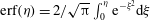 $\text{erf}({\it\eta})=2/\sqrt{{\rm\pi}}\int _{0}^{{\it\eta}}\text{e}^{-{\it\xi}^{2}}\text{d}{\it\xi}$
. The equation is recast in terms of
$\text{erf}({\it\eta})=2/\sqrt{{\rm\pi}}\int _{0}^{{\it\eta}}\text{e}^{-{\it\xi}^{2}}\text{d}{\it\xi}$
. The equation is recast in terms of
 $\bar{u}^{\wedge }$
,
$\bar{u}^{\wedge }$
,
 $y^{+0}$
and
$y^{+0}$
and
 $t^{+0}$
for plotting. It is clear that, visually, the time-developing boundary layer shows strong similarities to the spatially developing boundary layer. Most interestingly, the profiles in different cases collapse closely on top of each other for
$t^{+0}$
for plotting. It is clear that, visually, the time-developing boundary layer shows strong similarities to the spatially developing boundary layer. Most interestingly, the profiles in different cases collapse closely on top of each other for
 $t^{+0}<100$
(that is, in the pre-transition stage). At earlier stages (say,
$t^{+0}<100$
(that is, in the pre-transition stage). At earlier stages (say,
 $t^{+0}<50$
), these velocity profiles are closely represented by the Stokes solution. Later,
$t^{+0}<50$
), these velocity profiles are closely represented by the Stokes solution. Later,
 $50<t^{+0}<100$
, the profiles of the various cases are still in close agreement with each other, but they deviate from the Stokes solution. Further proceeding with time (say
$50<t^{+0}<100$
, the profiles of the various cases are still in close agreement with each other, but they deviate from the Stokes solution. Further proceeding with time (say
 $t^{+0}>110$
), the profiles of the various cases start diverge from each other. The close accordance between the velocity developments of the various flow cases during the pre-transition phase is extraordinary, noting the wide range of Reynolds number ratios examined. The response of the mean velocity in the transient flow is the same in a 10 % increase flow as in a 400 % increase one, irrespective of their very different flow patterns shown in figure 1, for example. Further, the profiles of the velocity
$t^{+0}>110$
), the profiles of the various cases start diverge from each other. The close accordance between the velocity developments of the various flow cases during the pre-transition phase is extraordinary, noting the wide range of Reynolds number ratios examined. The response of the mean velocity in the transient flow is the same in a 10 % increase flow as in a 400 % increase one, irrespective of their very different flow patterns shown in figure 1, for example. Further, the profiles of the velocity
 $\bar{u}^{\wedge }$
with respect to the non-dimensional parameter
$\bar{u}^{\wedge }$
with respect to the non-dimensional parameter
 ${\it\eta}$
at various times of the pre-transitional phase (
${\it\eta}$
at various times of the pre-transitional phase (
 $t^{+0}<80$
) in all the cases are shown in figure 6(b) together with the Stokes solution. It can be seen that the profiles collapse very well onto a single curve, close to the Stokes solution, with only small spreads, hence showing the similarity of the velocity profiles at different times. Figure 7 shows that the values of the displacement thickness
$t^{+0}<80$
) in all the cases are shown in figure 6(b) together with the Stokes solution. It can be seen that the profiles collapse very well onto a single curve, close to the Stokes solution, with only small spreads, hence showing the similarity of the velocity profiles at different times. Figure 7 shows that the values of the displacement thickness
 $({\it\delta}^{\ast })$
of the perturbation velocity in the various cases correlates reasonably well when they are normalized by the initial flow wall units, that is,
$({\it\delta}^{\ast })$
of the perturbation velocity in the various cases correlates reasonably well when they are normalized by the initial flow wall units, that is,
 ${\it\delta}^{\ast +0}={\it\delta}^{\ast }u_{{\it\tau}0}/{\it\nu}$
.
${\it\delta}^{\ast +0}={\it\delta}^{\ast }u_{{\it\tau}0}/{\it\nu}$
.
Displacement thickness of the perturbation velocity (
 $\bar{u}^{\wedge }$
).
$\bar{u}^{\wedge }$
).

Development of the modified friction coefficient
 $C_{f,du}^{\prime }$
defined by (3.14) with non-dimensional time
$C_{f,du}^{\prime }$
defined by (3.14) with non-dimensional time
 $t^{+0}$
in all cases.
$t^{+0}$
in all cases.

A friction coefficient for the perturbation flow can be defined as
 $$\begin{eqnarray}C_{f,du}=\frac{{\it\tau}_{w,du}}{\displaystyle {\textstyle \frac{1}{2}}{\it\rho}\left(U_{b1}-U_{b0}\right)^{2}},\end{eqnarray}$$
where
 ${\it\tau}_{w,du}=\{{\it\mu}\partial [\bar{u}(y,t^{\ast })-\bar{u}(y,0)]/\partial y\}|_{y=0}={\it\tau}_{w}-{\it\tau}_{w,0}$
is the wall shear stress of the perturbation flow, and
${\it\tau}_{w,du}=\{{\it\mu}\partial [\bar{u}(y,t^{\ast })-\bar{u}(y,0)]/\partial y\}|_{y=0}={\it\tau}_{w}-{\it\tau}_{w,0}$
is the wall shear stress of the perturbation flow, and
 ${\it\tau}_{w}$
and
${\it\tau}_{w}$
and
 ${\it\tau}_{w,0}$
are the values of the wall shear stress of the full flow at times
${\it\tau}_{w,0}$
are the values of the wall shear stress of the full flow at times
 $t$
and 0 respectively. Noting that the wall shear stress of the theoretical solution of Stokes’ first problem is
$t$
and 0 respectively. Noting that the wall shear stress of the theoretical solution of Stokes’ first problem is
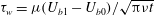 ${\it\tau}_{w}={\it\mu}(U_{b1}-U_{b0})/\sqrt{{\rm\pi}{\it\nu}t}$
(Schlichting & Gersten Reference Schlichting and Gersten2000), the friction coefficient for a transient laminar flow is given by
${\it\tau}_{w}={\it\mu}(U_{b1}-U_{b0})/\sqrt{{\rm\pi}{\it\nu}t}$
(Schlichting & Gersten Reference Schlichting and Gersten2000), the friction coefficient for a transient laminar flow is given by
 $$\begin{eqnarray}C_{f,Stokes}=\frac{2}{\sqrt{{\rm\pi}}}\frac{1}{\displaystyle \sqrt{\frac{\left(U_{b1}-U_{b0}\right)^{2}t}{{\it\nu}}}}.\end{eqnarray}$$
Now, returning to the data shown in figure 6(a), the fact that the velocity profiles of the various cases overlap each other at any
 $t^{+0}$
implies that the values of the wall shear stress of
$t^{+0}$
implies that the values of the wall shear stress of
 $\bar{u}^{\wedge }$
normalized in the manner defined below should collapse on top of each other when expressed in terms of
$\bar{u}^{\wedge }$
normalized in the manner defined below should collapse on top of each other when expressed in terms of
 $t^{+0}$
:
$t^{+0}$
:
 $$\begin{eqnarray}C_{f,du}^{\prime }=\frac{{\it\tau}_{w,du}}{\displaystyle {\textstyle \frac{1}{2}}{\it\rho}\left(U_{b1}-U_{b0}\right)u_{{\it\tau}0}},\end{eqnarray}$$
which can be reorganized as
 $$\begin{eqnarray}C_{f,du}^{\prime }=C_{f,du}\frac{\left(U_{b1}-U_{b0}\right)}{u_{{\it\tau}0}}.\end{eqnarray}$$
The present data in the form of the modified friction coefficient
 $C_{f,du}^{\prime }$
defined above plotted against
$C_{f,du}^{\prime }$
defined above plotted against
 $t^{+0}$
are shown in figure 8, together with the Stokes solution for comparison. It can be seen that all the data indeed collapse well onto a single curve during the pre-transitional stage. This curve is elevated from the Stokes solution, but can be well represented by the following expression:
$t^{+0}$
are shown in figure 8, together with the Stokes solution for comparison. It can be seen that all the data indeed collapse well onto a single curve during the pre-transitional stage. This curve is elevated from the Stokes solution, but can be well represented by the following expression:
 $$\begin{eqnarray}C_{f,du}^{\prime }=\frac{2}{\sqrt{{\rm\pi}}}\frac{1}{\left(t^{+0}\right)^{0.47}},\end{eqnarray}$$
which is shown in the figure. The expression can be recast in terms of
 $C_{f,du}$
as
$C_{f,du}$
as
 $$\begin{eqnarray}C_{f,du}=\frac{2}{\sqrt{{\rm\pi}}}\frac{(t^{+0})^{0.03}}{\displaystyle \sqrt{\frac{\left(U_{b1}-U_{b0}\right)^{2}t}{{\it\nu}}}}=C_{f,Stokes}(t^{+0})^{0.03}.\end{eqnarray}$$
Equation (3.16) together with figure 8 demonstrates that the detailed variation of the wall shear stress in the pre-transient phase of all the transient flow cases can be closely correlated in terms of the modified friction coefficient (
 $C_{f,du}^{\prime }$
) against the wall-unit time of the initial flow (
$C_{f,du}^{\prime }$
) against the wall-unit time of the initial flow (
 $t^{+0}$
). This correlation deviates somewhat from the solution of Stokes’ first problem for laminar flow, but only needs a relatively small correction based on
$t^{+0}$
). This correlation deviates somewhat from the solution of Stokes’ first problem for laminar flow, but only needs a relatively small correction based on
 $t^{+0}$
. In practice, either (3.16) or (3.17) can be used to predict the wall shear stress in a transient turbulent flow. Another useful piece of information that can be derived from figure 8 is that the timing of the onset of transition in terms of
$t^{+0}$
. In practice, either (3.16) or (3.17) can be used to predict the wall shear stress in a transient turbulent flow. Another useful piece of information that can be derived from figure 8 is that the timing of the onset of transition in terms of
 $t^{+0}$
does not change significantly as the flow conditions are varied, being in the range of
$t^{+0}$
does not change significantly as the flow conditions are varied, being in the range of
 $t^{+0}=80{-}110$
for the conditions examined in this study. As a result,
$t^{+0}=80{-}110$
for the conditions examined in this study. As a result,
 $t^{+0}$
provides a good measure of the stage of the flow development, and hence the reason for using it for comparison for the flow developments under the various conditions.
$t^{+0}$
provides a good measure of the stage of the flow development, and hence the reason for using it for comparison for the flow developments under the various conditions.
Development of the profiles of
 $u_{rms}^{\prime }$
,
$u_{rms}^{\prime }$
,
 $v_{rms}^{\prime }$
,
$v_{rms}^{\prime }$
,
 $w_{rms}^{\prime }$
at various times. The profiles are shifted to the right by a distance proportional to the time. (a) S11; (b) S15. Thin lines: initial profiles; thick lines: profiles at time
$w_{rms}^{\prime }$
at various times. The profiles are shifted to the right by a distance proportional to the time. (a) S11; (b) S15. Thin lines: initial profiles; thick lines: profiles at time
 $t^{+0}$
; lower horizontal lines: displacement boundary layer (
$t^{+0}$
; lower horizontal lines: displacement boundary layer (
 ${\it\delta}^{\ast }$
); higher horizontal lines: velocity boundary layer (
${\it\delta}^{\ast }$
); higher horizontal lines: velocity boundary layer (
 ${\it\delta}_{99}$
).
${\it\delta}_{99}$
).

3.4. Energy growth
Figure 9 shows the development of the profiles of
 $u_{rms}^{\prime }$
,
$u_{rms}^{\prime }$
,
 $v_{rms}^{\prime }$
and
$v_{rms}^{\prime }$
and
 $w_{rms}^{\prime }$
in S11 and S15 for Reynolds number ratios of 4.5 and 1.25 respectively, to represent a low- and a high-FST case. The profiles at any time
$w_{rms}^{\prime }$
in S11 and S15 for Reynolds number ratios of 4.5 and 1.25 respectively, to represent a low- and a high-FST case. The profiles at any time
 $t^{+0}$
are shifted by a distance proportional to
$t^{+0}$
are shifted by a distance proportional to
 $t^{+0}$
. Despite the large differences in the level of the changes in the two cases, some features of the response of turbulence can be identified in both scenarios, which are also common in all other cases. (i) The value of
$t^{+0}$
. Despite the large differences in the level of the changes in the two cases, some features of the response of turbulence can be identified in both scenarios, which are also common in all other cases. (i) The value of
 $u_{rms}^{\prime }$
starts to increase from the start of the transient, reaching a level that is close to the maximum value at the time of the onset of transition, only making slow adjustments afterwards. The pre-transition rapid increase is an important feature of transition, which reflects the formation and enhancement of the streaky structures, and is comparable to the pre-transitional energy growth in a boundary layer. (ii) By contrast,
$u_{rms}^{\prime }$
starts to increase from the start of the transient, reaching a level that is close to the maximum value at the time of the onset of transition, only making slow adjustments afterwards. The pre-transition rapid increase is an important feature of transition, which reflects the formation and enhancement of the streaky structures, and is comparable to the pre-transitional energy growth in a boundary layer. (ii) By contrast,
 $v_{rms}^{\prime }$
and
$v_{rms}^{\prime }$
and
 $w_{rms}^{\prime }$
remain largely unchanged (in fact reduce very slightly, as shown below) during the pre-transition period. They only start to increase when transition occurs.
$w_{rms}^{\prime }$
remain largely unchanged (in fact reduce very slightly, as shown below) during the pre-transition period. They only start to increase when transition occurs.
To facilitate a direct comparison between the energy growths in the various cases, the development of the profile of
 $(u_{rms}^{\prime }-u_{rms,0}^{\prime })$
normalized by the increase of the bulk velocity (
$(u_{rms}^{\prime }-u_{rms,0}^{\prime })$
normalized by the increase of the bulk velocity (
 $U_{b1}{-}U_{b0}$
) for all cases is shown in figure 10(a). It is clear that the profiles for all cases at any
$U_{b1}{-}U_{b0}$
) for all cases is shown in figure 10(a). It is clear that the profiles for all cases at any
 $t^{+0}$
agree very well with each other. In fact, the cases with the same final Reynolds number (series
$t^{+0}$
agree very well with each other. In fact, the cases with the same final Reynolds number (series
 $\text{S}0X$
) fall rather closely on top of each other, whereas the scattered points shown in the figure have largely originated from series
$\text{S}0X$
) fall rather closely on top of each other, whereas the scattered points shown in the figure have largely originated from series
 $\text{S}1X$
with a variation in the final Reynolds number, reflecting some albeit small unaccounted effect of
$\text{S}1X$
with a variation in the final Reynolds number, reflecting some albeit small unaccounted effect of
 $\mathit{Re}_{1}$
. Nevertheless, the close correlation is remarkable considering the fact that in some cases the flow is increased by only a very small amount, and that the flow structures appear to be so different between the cases, as shown in figure 1. Whether the flow shows strong or weak streaks, or even no streaks, the energy growth is apparently described by the same non-dimensional parameter. Also remarkable are the responses of
$\mathit{Re}_{1}$
. Nevertheless, the close correlation is remarkable considering the fact that in some cases the flow is increased by only a very small amount, and that the flow structures appear to be so different between the cases, as shown in figure 1. Whether the flow shows strong or weak streaks, or even no streaks, the energy growth is apparently described by the same non-dimensional parameter. Also remarkable are the responses of
 $v_{rms}^{\prime }$
shown in figure 10(b). During the most part of the pre-transition stage,
$v_{rms}^{\prime }$
shown in figure 10(b). During the most part of the pre-transition stage,
 $v_{rms}^{\prime }$
decreases slightly in all cases although only slightly, and then increases rapidly after approximately
$v_{rms}^{\prime }$
decreases slightly in all cases although only slightly, and then increases rapidly after approximately
 $t^{+0}=80$
. The
$t^{+0}=80$
. The
 $w_{rms}^{\prime }$
component shows a similar trend to
$w_{rms}^{\prime }$
component shows a similar trend to
 $v_{rms}^{\prime }$
(not shown). These results demonstrate that, even though the transition is very difficult to observe through visualizations in cases such as S16 due to the very small increase in flow rate, the process of a distinct quiescent pre-transition period followed by a ‘sudden’ and rapid generation of turbulence exhibits itself unambiguously in all cases in the turbulence statistics as well as in the velocity profiles discussed earlier.
$v_{rms}^{\prime }$
(not shown). These results demonstrate that, even though the transition is very difficult to observe through visualizations in cases such as S16 due to the very small increase in flow rate, the process of a distinct quiescent pre-transition period followed by a ‘sudden’ and rapid generation of turbulence exhibits itself unambiguously in all cases in the turbulence statistics as well as in the velocity profiles discussed earlier.
Development of the profiles of (a)
 $u_{rms}^{\prime \wedge }\,[=(u_{rms}^{\prime }-u_{rms,0}^{\prime })/(U_{b1}-U_{b0})]$
and (b)
$u_{rms}^{\prime \wedge }\,[=(u_{rms}^{\prime }-u_{rms,0}^{\prime })/(U_{b1}-U_{b0})]$
and (b)
 $v_{rms}^{\prime \wedge }\,[=(v_{rms}^{\prime }-v_{rms,0}^{\prime })/(U_{b1}-U_{b0})]$
at various times in the pre-transition period for all cases.
$v_{rms}^{\prime \wedge }\,[=(v_{rms}^{\prime }-v_{rms,0}^{\prime })/(U_{b1}-U_{b0})]$
at various times in the pre-transition period for all cases.

The maximum streamwise energy growth,
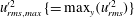 $u_{rms,max}^{\prime 2}\,\{=\max _{y}(u_{rms}^{\prime 2})\}$
, with respect to
$u_{rms,max}^{\prime 2}\,\{=\max _{y}(u_{rms}^{\prime 2})\}$
, with respect to
 $\mathit{Re}_{t}$
, is shown in figure 11(a). It is clear that the growth rate increases with increase of
$\mathit{Re}_{t}$
, is shown in figure 11(a). It is clear that the growth rate increases with increase of
 $\mathit{Tu}$
, which is consistent with the trend exhibited in the experiments by Fransson et al. (Reference Fransson, Matsubara and Alfredsson2005). Inspired by figure 10(a), the energy growth in terms of
$\mathit{Tu}$
, which is consistent with the trend exhibited in the experiments by Fransson et al. (Reference Fransson, Matsubara and Alfredsson2005). Inspired by figure 10(a), the energy growth in terms of
 ${\rm\Delta}E=\max _{y}\{(u_{rms}^{\prime }-u_{rms,0}^{\prime })^{2}/(U_{b1}-U_{b0})^{2}\}$
is plotted against
${\rm\Delta}E=\max _{y}\{(u_{rms}^{\prime }-u_{rms,0}^{\prime })^{2}/(U_{b1}-U_{b0})^{2}\}$
is plotted against
 $t^{+0}$
(figure 11
b). Again, the data from the series
$t^{+0}$
(figure 11
b). Again, the data from the series
 $\text{S}0X$
practically collapse on top of each other whereas the data from
$\text{S}0X$
practically collapse on top of each other whereas the data from
 $\text{S}1X$
have some deviations from the overall trend but still follow it rather closely. At the very early stage, there is a ‘delay’ in the increase of the energy, which was also noted by Fransson et al. (Reference Fransson, Matsubara and Alfredsson2005), who attributed it to an early receptivity stage when the flow adjusts itself to the boundary layer. Following this stage, the energy growth is linear, which in many cases extends much beyond the point of the onset of transition. Noting that
$\text{S}1X$
have some deviations from the overall trend but still follow it rather closely. At the very early stage, there is a ‘delay’ in the increase of the energy, which was also noted by Fransson et al. (Reference Fransson, Matsubara and Alfredsson2005), who attributed it to an early receptivity stage when the flow adjusts itself to the boundary layer. Following this stage, the energy growth is linear, which in many cases extends much beyond the point of the onset of transition. Noting that
 $u_{{\it\tau}0}/U_{b1}=((u_{rms,0}^{\prime })_{max}/U_{b1})(u_{{\it\tau}0}/(u_{rms,0}^{\prime })_{max})=\mathit{Tu}_{0}/(u_{rms,0}^{\prime +})_{max}$
and that
$u_{{\it\tau}0}/U_{b1}=((u_{rms,0}^{\prime })_{max}/U_{b1})(u_{{\it\tau}0}/(u_{rms,0}^{\prime })_{max})=\mathit{Tu}_{0}/(u_{rms,0}^{\prime +})_{max}$
and that
 $(u_{rms,0}^{\prime +})_{max}$
is only a very weak function of the Reynolds number,
$(u_{rms,0}^{\prime +})_{max}$
is only a very weak function of the Reynolds number,
 $t^{+0}=(tu_{{\it\tau}0}^{2}/{\it\nu})=(tU_{b1}^{2}/{\it\nu})(u_{{\it\tau}0}^{2}/U_{b1}^{2})\propto \mathit{Re}_{t}\mathit{Tu}_{0}^{2}$
. Consequently, figure 11(b) implies that
$t^{+0}=(tu_{{\it\tau}0}^{2}/{\it\nu})=(tU_{b1}^{2}/{\it\nu})(u_{{\it\tau}0}^{2}/U_{b1}^{2})\propto \mathit{Re}_{t}\mathit{Tu}_{0}^{2}$
. Consequently, figure 11(b) implies that
 $$\begin{eqnarray}{\rm\Delta}E\propto \mathit{Re}_{t}\mathit{Tu}_{0}^{2}.\end{eqnarray}$$
That is, the energy growth is linearly proportional to the initial FST intensity squared when
 $\mathit{Re}_{t}$
is fixed, or vice versa. The same expression has been reached by Fransson et al. (Reference Fransson, Matsubara and Alfredsson2005) based on their boundary layer experimental data. It should be noted that, strictly speaking,
$\mathit{Re}_{t}$
is fixed, or vice versa. The same expression has been reached by Fransson et al. (Reference Fransson, Matsubara and Alfredsson2005) based on their boundary layer experimental data. It should be noted that, strictly speaking,
 ${\rm\Delta}E$
is not the energy growth. Either
${\rm\Delta}E$
is not the energy growth. Either
 $u_{rms}^{\prime 2}$
or
$u_{rms}^{\prime 2}$
or
 $u_{rms}^{\prime 2}-u_{rms,0}^{\prime 2}$
instead of
$u_{rms}^{\prime 2}-u_{rms,0}^{\prime 2}$
instead of
 $(u_{rms}^{\prime }-u_{rms,0}^{\prime })^{2}$
would be a better representation of the energy in defining
$(u_{rms}^{\prime }-u_{rms,0}^{\prime })^{2}$
would be a better representation of the energy in defining
 ${\rm\Delta}E$
, but no correlation can be found in these forms. This suggests that there may exist some nonlinear interactions between the existing flow structure and the growth of the ‘disturbances’.
${\rm\Delta}E$
, but no correlation can be found in these forms. This suggests that there may exist some nonlinear interactions between the existing flow structure and the growth of the ‘disturbances’.
Energy growth: (a)
 $u_{rms,max}^{\prime 2}/U_{b1}^{2}$
versus
$u_{rms,max}^{\prime 2}/U_{b1}^{2}$
versus
 $\mathit{Re}_{t}$
, (b)
$\mathit{Re}_{t}$
, (b)
 ${\rm\Delta}E=\max _{y}\{(u_{rms}^{\prime }-u_{rms,0}^{\prime })^{2}/(U_{b1}-U_{b0})^{2}\}$
versus
${\rm\Delta}E=\max _{y}\{(u_{rms}^{\prime }-u_{rms,0}^{\prime })^{2}/(U_{b1}-U_{b0})^{2}\}$
versus
 $t^{+0}$
.
$t^{+0}$
.

Figure 12 shows the profiles of
 $u_{rms}^{\prime }$
normalized by its maximum value plotted against
$u_{rms}^{\prime }$
normalized by its maximum value plotted against
 $y/{\it\delta}_{u}^{\ast }$
for a number of cases, where
$y/{\it\delta}_{u}^{\ast }$
for a number of cases, where
 ${\it\delta}_{u}^{\ast }$
is the displacement thickness of the full velocity profile (i.e.
${\it\delta}_{u}^{\ast }$
is the displacement thickness of the full velocity profile (i.e.
 $\bar{u}$
not
$\bar{u}$
not
 $\bar{u}^{\wedge }$
). For the cases shown in figure 12(a), it is clear that the peak location remains fixed during the pre-transition period, where the profiles show close similarity. During the transition period, the peak location moves towards the wall. For the cases with a small Reynolds number ratio (figure 12
b), the change of the peak location is small throughout the transient period. Although the peak location remains fixed during the pre-transition for each flow, it is different for different flows, varying from 0.85 for S11 to 0.57 for S16 as the final Reynolds number reduces. This is in contrast to the boundary layer transition, in which the peak location is always at
$\bar{u}^{\wedge }$
). For the cases shown in figure 12(a), it is clear that the peak location remains fixed during the pre-transition period, where the profiles show close similarity. During the transition period, the peak location moves towards the wall. For the cases with a small Reynolds number ratio (figure 12
b), the change of the peak location is small throughout the transient period. Although the peak location remains fixed during the pre-transition for each flow, it is different for different flows, varying from 0.85 for S11 to 0.57 for S16 as the final Reynolds number reduces. This is in contrast to the boundary layer transition, in which the peak location is always at
 $y/{\it\delta}^{\ast }=1.3$
, which has been derived from optimal growth theory (Andersson et al.
Reference Andersson, Berggren and Henningson1999) and demonstrated by DNS and experiments (e.g. Matsubara & Alfredsson Reference Matsubara and Alfredsson2001; Brandt et al.
Reference Brandt, Schlatter and Henningson2004). A major reason for the transient channel to be different is likely to be associated with the fact that the free-stream velocity is not a flat profile but varies with the distance from the wall.
$y/{\it\delta}^{\ast }=1.3$
, which has been derived from optimal growth theory (Andersson et al.
Reference Andersson, Berggren and Henningson1999) and demonstrated by DNS and experiments (e.g. Matsubara & Alfredsson Reference Matsubara and Alfredsson2001; Brandt et al.
Reference Brandt, Schlatter and Henningson2004). A major reason for the transient channel to be different is likely to be associated with the fact that the free-stream velocity is not a flat profile but varies with the distance from the wall.
Profiles of streamwise r.m.s. velocity normalized by its peak value at several instants. Solid lines with markers: initial profile; solid lines: pre-transitional period (
 $t^{+0}<100$
); dashed lines: transitional and turbulent periods (
$t^{+0}<100$
); dashed lines: transitional and turbulent periods (
 $t^{+0}>100$
).
$t^{+0}>100$
).

Time variation of the spanwise correlation of the streamwise velocity at a plane
 $y^{+0}=0.5$
(the magnitude of negative correlations is shown; positive correlations are set to zero).
$y^{+0}=0.5$
(the magnitude of negative correlations is shown; positive correlations are set to zero).

3.5. Flow structures
Due to the presence of high- and low-speed streaks in turbulent and transitional flows, the spanwise correlation of the streamwise velocity (
 $R_{11}$
) shows a negative peak, a phenomenon that is commonly used to illustrate the behaviour of the streaks. A higher value of the negative peak of the correlation,
$R_{11}$
) shows a negative peak, a phenomenon that is commonly used to illustrate the behaviour of the streaks. A higher value of the negative peak of the correlation,
 $|R_{11,min}|$
, can be associated with the existence of stronger and/or more regularly spaced streaks relative to the background disturbances. Furthermore, the ‘
$|R_{11,min}|$
, can be associated with the existence of stronger and/or more regularly spaced streaks relative to the background disturbances. Furthermore, the ‘
 $y$
’ location of the peak negative correlation (
$y$
’ location of the peak negative correlation (
 $y_{min}$
) indicates the averaged central location of the streaks above the wall. Twice the
$y_{min}$
) indicates the averaged central location of the streaks above the wall. Twice the
 $z$
value at which this occurs (
$z$
value at which this occurs (
 $z_{min}$
) can be seen as a measure of the averaged streak spacing. Figure 13 shows the time variation of the spanwise correlation on a horizontal plane near the wall (
$z_{min}$
) can be seen as a measure of the averaged streak spacing. Figure 13 shows the time variation of the spanwise correlation on a horizontal plane near the wall (
 $y^{+0}=0.5$
) for various cases with the steady flow values shown in
$y^{+0}=0.5$
) for various cases with the steady flow values shown in
 $t^{+0}<0$
. The absolute values of the negative correlations are shown while the positive correlations are set to zero for clarity. The overall behaviour of the streaks during the transient flows is well displayed. The streaks are enhanced relative to the background turbulence (that is,
$t^{+0}<0$
. The absolute values of the negative correlations are shown while the positive correlations are set to zero for clarity. The overall behaviour of the streaks during the transient flows is well displayed. The streaks are enhanced relative to the background turbulence (that is,
 $|R_{11,min}|$
is greater) during the pre-transition period in all cases, but much more strongly in some than in others. The streak spacing appears to reduce initially but then mostly stay unchanged during the pre-transition period. The ‘strength’ and location/spacing of the streaks are quantified next: the variations of the minimum value (
$|R_{11,min}|$
is greater) during the pre-transition period in all cases, but much more strongly in some than in others. The streak spacing appears to reduce initially but then mostly stay unchanged during the pre-transition period. The ‘strength’ and location/spacing of the streaks are quantified next: the variations of the minimum value (
 $|R_{11,min}|$
) with time for all cases are shown in figure 14, and the time variations of the wall-normal distance (
$|R_{11,min}|$
) with time for all cases are shown in figure 14, and the time variations of the wall-normal distance (
 $y_{min}$
) as well as the spanwise location (
$y_{min}$
) as well as the spanwise location (
 $z_{min}$
) are shown in figure 15.
$z_{min}$
) are shown in figure 15.
Development of the minimum spanwise correlation of the streamwise velocity for streaks close to the wall (
 $y<0.2$
). Lines only:
$y<0.2$
). Lines only:
 $\text{S}1X$
series; lines and markers:
$\text{S}1X$
series; lines and markers:
 $\text{S}0X$
series.
$\text{S}0X$
series.

Development of the wall-normal distance (
 $y_{min}$
) and spanwise location (
$y_{min}$
) and spanwise location (
 $z_{min}$
) of the strongest near-wall streaks (
$z_{min}$
) of the strongest near-wall streaks (
 $y<0.2$
) normalized with inner and outer length scales. Lines only:
$y<0.2$
) normalized with inner and outer length scales. Lines only:
 $\text{S}1X$
series; lines and markers:
$\text{S}1X$
series; lines and markers:
 $\text{S}0X$
series.
$\text{S}0X$
series.

The general trend of the variation of
 $|R_{11,min}|$
is similar in the various cases. It first increases, reaching a peak at approximately
$|R_{11,min}|$
is similar in the various cases. It first increases, reaching a peak at approximately
 $t^{+0}=50{-}70$
, and reduces thereafter. The increase of
$t^{+0}=50{-}70$
, and reduces thereafter. The increase of
 $|R_{11,min}|$
is greater with increasing
$|R_{11,min}|$
is greater with increasing
 $\mathit{Tu}_{0}$
in both series, but the final value in most cases in
$\mathit{Tu}_{0}$
in both series, but the final value in most cases in
 $\text{S}0X$
is much lower due to their starting point (i.e. the streaks are weaker and/or fewer at higher Reynolds numbers). On the other hand, there appears to be an absolute maximum in
$\text{S}0X$
is much lower due to their starting point (i.e. the streaks are weaker and/or fewer at higher Reynolds numbers). On the other hand, there appears to be an absolute maximum in
 $|R_{11,min}|$
, just below 0.3, which has been reached in S01, S11 and S12. For these three cases, the streak strength reduces sharply at the time of the onset of transition, reaching a minimum value towards the end of the transition. This is consistent with the visualization of the flow field in figure 1(a), namely strong streaks are formed during the pre-transition phase, but destroyed during transition as turbulence spots are generated and spread. By contrast, in the cases of a low Reynolds number ratio, such as in S15 and S16, the strengthening of the streaks is minor, and, probably more significantly, the streaks are only slightly weakened during the period of transition. It is hence likely that streak formation and instability are not the dominant mechanisms under such flow conditions. The change from streak-dominated to streak-‘inactive’ cases appears to be progressive as the Reynolds number ratio is decreased and hence no sudden transition from one mode to the other is displayed.
$|R_{11,min}|$
, just below 0.3, which has been reached in S01, S11 and S12. For these three cases, the streak strength reduces sharply at the time of the onset of transition, reaching a minimum value towards the end of the transition. This is consistent with the visualization of the flow field in figure 1(a), namely strong streaks are formed during the pre-transition phase, but destroyed during transition as turbulence spots are generated and spread. By contrast, in the cases of a low Reynolds number ratio, such as in S15 and S16, the strengthening of the streaks is minor, and, probably more significantly, the streaks are only slightly weakened during the period of transition. It is hence likely that streak formation and instability are not the dominant mechanisms under such flow conditions. The change from streak-dominated to streak-‘inactive’ cases appears to be progressive as the Reynolds number ratio is decreased and hence no sudden transition from one mode to the other is displayed.
It can be seen from figure 15(a) that the
 $z$
-location of the minimum correlation, or the half-streak spacing, normalized with the initial-flow wall units (
$z$
-location of the minimum correlation, or the half-streak spacing, normalized with the initial-flow wall units (
 $z_{min}^{+0}$
), initially reduces rapidly after the commencement of the transient flow, by an amount that is roughly proportional to the Reynolds number ratio of the flow. It then remains as a constant until the onset of transition, implying that the streak spacing in absolute terms remains unchanged during the most part of the pre-transitional phase, noting that the normalization is based on the initial flow and remains unchanged during the transition. The initial and final streak spacings (
$z_{min}^{+0}$
), initially reduces rapidly after the commencement of the transient flow, by an amount that is roughly proportional to the Reynolds number ratio of the flow. It then remains as a constant until the onset of transition, implying that the streak spacing in absolute terms remains unchanged during the most part of the pre-transitional phase, noting that the normalization is based on the initial flow and remains unchanged during the transition. The initial and final streak spacings (
 $2z_{min}^{+}$
) based on their respective wall units of the flow are both approximately 100, as expected for an equilibrium turbulent flow (the latter is not shown). When expressed with respect to the displacement thickness of the full flow field,
$2z_{min}^{+}$
) based on their respective wall units of the flow are both approximately 100, as expected for an equilibrium turbulent flow (the latter is not shown). When expressed with respect to the displacement thickness of the full flow field,
 $z_{min}/{\it\delta}_{u}^{\ast }$
(figure 15
b), the distance of the minimum location in different cases reduces from various initial values during the pre-transition period, converging to approximately 2.5 at the point of onset of transition for the
$z_{min}/{\it\delta}_{u}^{\ast }$
(figure 15
b), the distance of the minimum location in different cases reduces from various initial values during the pre-transition period, converging to approximately 2.5 at the point of onset of transition for the
 $\text{S}1X$
series where
$\text{S}1X$
series where
 $\mathit{Re}_{0}$
is maintained the same, but to different values for
$\mathit{Re}_{0}$
is maintained the same, but to different values for
 $\text{S}0X$
where
$\text{S}0X$
where
 $\mathit{Re}_{1}$
is the same. These results compare favourably with those of Ovchinnikov et al. (Reference Ovchinnikov, Choudhari and Piomelli2008) for bypass transition; they have shown that the absolute streak spacing remains unchanged for a period during the pre-transition stage, but the value is different for FSTs with different amplitudes or length scales. They showed that
$\mathit{Re}_{1}$
is the same. These results compare favourably with those of Ovchinnikov et al. (Reference Ovchinnikov, Choudhari and Piomelli2008) for bypass transition; they have shown that the absolute streak spacing remains unchanged for a period during the pre-transition stage, but the value is different for FSTs with different amplitudes or length scales. They showed that
 $z_{min}/{\it\delta}_{u}^{\ast }$
in their cases reduces to converge to approximately 2 in most cases, whereas the experimental data of Matsubara & Alfredsson (Reference Matsubara and Alfredsson2001) found that it tends to 3.
$z_{min}/{\it\delta}_{u}^{\ast }$
in their cases reduces to converge to approximately 2 in most cases, whereas the experimental data of Matsubara & Alfredsson (Reference Matsubara and Alfredsson2001) found that it tends to 3.
The wall-normal distance of the location of the minimum correlation coefficient normalized using the initial-flow wall units (
 $y_{min}^{+0}$
) behaves in a very similar way in all the cases (figure 15
c). Following a brief reduction from its initial value of approximately 10, it increases roughly linearly throughout the pre-transition phase and approaches a value between 12 and 14 just before the onset of transition. The location in relation to the momentum displacement thickness (
$y_{min}^{+0}$
) behaves in a very similar way in all the cases (figure 15
c). Following a brief reduction from its initial value of approximately 10, it increases roughly linearly throughout the pre-transition phase and approaches a value between 12 and 14 just before the onset of transition. The location in relation to the momentum displacement thickness (
 ${\it\delta}_{u}^{\ast }$
) in each case also increases, but only slightly (figure 15
d), and more significantly it assumes very different values for different cases, spreading from approximately 0.3 to nearly 1. The implication is that the streaks lift up in both absolute terms and relative to the boundary layer, but the former is more significant.
${\it\delta}_{u}^{\ast }$
) in each case also increases, but only slightly (figure 15
d), and more significantly it assumes very different values for different cases, spreading from approximately 0.3 to nearly 1. The implication is that the streaks lift up in both absolute terms and relative to the boundary layer, but the former is more significant.
The peak values of the streaks are naturally much greater than the r.m.s. values of the corresponding fluctuating velocities and Wundrow & Goldstein (Reference Wundrow and Goldstein2001) suggested that it is likely that the strong events that are associated with these peaks are relevant to the onset of instability rather than the mean values. Hence the fact that experiments often report that r.m.s. values may be a major contributing factor to the differences often observed between the theory and measurements in levels of disturbance energy at the onset of transition. Brandt et al. (Reference Brandt, Schlatter and Henningson2004) and more recently Nolan & Zaki (Reference Nolan and Zaki2013) have further evaluated the idea and provided additional explanation and evidence. We represent the peak amplitudes of the streaks with the maximum and minimum fluctuating velocities defined as follows:
 $$\begin{eqnarray}\displaystyle & u_{max}^{\prime }(t)=\mathop{\max }_{y}\Big\{\!\mathop{\max }_{x,z}[u(x,y,z,t)-\langle u(y,t)\rangle ]\Big\}\Big/U_{b1}, & \displaystyle\end{eqnarray}$$
 $$\begin{eqnarray}\displaystyle & u_{min}^{\prime }(t)=\mathop{\min }_{y}\Big\{\!\mathop{\min }_{x,z}[u(x,y,z,t)-\langle u(y,t)\rangle ]\Big\}\Big/U_{b1}, & \displaystyle\end{eqnarray}$$
 $\langle u(y,t)\rangle$
denotes the span and streamwise average over a
$\langle u(y,t)\rangle$
denotes the span and streamwise average over a
 $y$
-plane. The
$y$
-plane. The
 $u_{max}^{\prime }$
and
$u_{max}^{\prime }$
and
 $u_{min}^{\prime }$
for the
$u_{min}^{\prime }$
for the
 $\text{S}0X$
and
$\text{S}0X$
and
 $\text{S}1X$
series are shown in figure 16. The initial value of
$\text{S}1X$
series are shown in figure 16. The initial value of
 $u_{max}^{\prime }$
varies in a wide range, from 0.1 to 0.5, among the various cases with a higher-Reynolds-number-ratio flow resulting in a lower
$u_{max}^{\prime }$
varies in a wide range, from 0.1 to 0.5, among the various cases with a higher-Reynolds-number-ratio flow resulting in a lower
 $u_{max}^{\prime }$
as expected. After the commencement of the transient, the cases with a lower initial value, however, increase faster than those with a higher initial value and, by the time of the onset of transition, all cases converge to a value of approximately 0.55. The
$u_{max}^{\prime }$
as expected. After the commencement of the transient, the cases with a lower initial value, however, increase faster than those with a higher initial value and, by the time of the onset of transition, all cases converge to a value of approximately 0.55. The
 $u_{min}^{\prime }$
tends to follow a similar trend but converges to a slightly smaller value of approximately
$u_{min}^{\prime }$
tends to follow a similar trend but converges to a slightly smaller value of approximately
 $-0.5$
. Incidentally, these values are comparable to the values 0.5 and
$-0.5$
. Incidentally, these values are comparable to the values 0.5 and
 $-0.45$
of Brandt et al. (Reference Brandt, Schlatter and Henningson2004) for boundary layers, which are taken from figure 7 of that paper. It is interesting to note that the
$-0.45$
of Brandt et al. (Reference Brandt, Schlatter and Henningson2004) for boundary layers, which are taken from figure 7 of that paper. It is interesting to note that the
 $u_{max}^{\prime }$
increases sharply at the time of the onset of transition in S11 and S12, and to a smaller extent in S01, but not in the remaining cases. This observation seems again to suggest that these three cases show different characteristics from the other cases. In fact, it is rather surprising that the streak peaks appear to reach approximately the same values in all flow cases around the time of the onset of transition, considering that streaks are probably not the dominant transition mechanism in some low-Reynolds-number-ratio cases. Figure 17 shows that, in the pre-transition stage, the wall-normal location at which the
$u_{max}^{\prime }$
increases sharply at the time of the onset of transition in S11 and S12, and to a smaller extent in S01, but not in the remaining cases. This observation seems again to suggest that these three cases show different characteristics from the other cases. In fact, it is rather surprising that the streak peaks appear to reach approximately the same values in all flow cases around the time of the onset of transition, considering that streaks are probably not the dominant transition mechanism in some low-Reynolds-number-ratio cases. Figure 17 shows that, in the pre-transition stage, the wall-normal location at which the
 $u_{min}^{\prime }$
occurs is approximately 3 times higher than that of
$u_{min}^{\prime }$
occurs is approximately 3 times higher than that of
 $u_{max}^{\prime }$
, indicating that high-speed streaks are located closer to the wall whereas low-speed streaks are pushed away from the wall, which is consistent with the results of Brandt et al. (Reference Brandt, Schlatter and Henningson2004).
$u_{max}^{\prime }$
, indicating that high-speed streaks are located closer to the wall whereas low-speed streaks are pushed away from the wall, which is consistent with the results of Brandt et al. (Reference Brandt, Schlatter and Henningson2004).
Development of the peak positive and negative streak amplitudes
 $u_{max}^{\prime }$
and
$u_{max}^{\prime }$
and
 $u_{min}^{\prime }$
: (a) and (c)
$u_{min}^{\prime }$
: (a) and (c)
 $\text{S}0X$
series; (b) and (d)
$\text{S}0X$
series; (b) and (d)
 $\text{S}1X$
series.
$\text{S}1X$
series.

Evolution of the locations of the peak positive and negative streaks,
 $(y/{\it\delta})_{+peaks}$
and
$(y/{\it\delta})_{+peaks}$
and
 $(y/{\it\delta})_{-peaks}$
: (a) and (c)
$(y/{\it\delta})_{-peaks}$
: (a) and (c)
 $\text{S}0X$
series; (b) and (d)
$\text{S}0X$
series; (b) and (d)
 $\text{S}1X$
series.
$\text{S}1X$
series.

Finally, it is of interest to inspect the flatness of
 $v^{\prime }$
, which responds strongly to the intermittence and hence provides a good measure of the strength of turbulent spots in comparison with the background turbulence. A large value of the flatness occurs when there is a small number of burst events, but each one, when it happens, has a high amplitude. Consequently, the peak of the flatness of
$v^{\prime }$
, which responds strongly to the intermittence and hence provides a good measure of the strength of turbulent spots in comparison with the background turbulence. A large value of the flatness occurs when there is a small number of burst events, but each one, when it happens, has a high amplitude. Consequently, the peak of the flatness of
 $v^{\prime }$
can be associated with the onset of transition. Figure 18 shows the flatness of
$v^{\prime }$
can be associated with the onset of transition. Figure 18 shows the flatness of
 $v^{\prime }$
at
$v^{\prime }$
at
 $y^{+0}=5$
in the various cases studied herein. In both the
$y^{+0}=5$
in the various cases studied herein. In both the
 $\text{S}0X$
and
$\text{S}0X$
and
 $\text{S}1X$
series, the peak value is the highest when the Reynolds number ratio is maximum, and reduces with decrease of the ratio. In consistency with the observations in figure 16, the peak values of S11 and S12 are much greater than those of the rest, being 1800 and 600 respectively, followed by 200 for S01. In addition, the period during which an increased value is observed is narrower, that is, the process is more abrupt, when the Reynolds number ratio is higher.
$\text{S}1X$
series, the peak value is the highest when the Reynolds number ratio is maximum, and reduces with decrease of the ratio. In consistency with the observations in figure 16, the peak values of S11 and S12 are much greater than those of the rest, being 1800 and 600 respectively, followed by 200 for S01. In addition, the period during which an increased value is observed is narrower, that is, the process is more abrupt, when the Reynolds number ratio is higher.
Development of flatness of the wall-normal velocity with non-dimensional time at
 $y^{+0}=5$
.
$y^{+0}=5$
.

4. Summary
Direct numerical simulations were performed of a transient flow in a channel following a step increase of flow rate from an initially turbulent flow. The aim was to study the transient behaviours under a range of initial (
 $\mathit{Re}_{0}$
) and final (
$\mathit{Re}_{0}$
) and final (
 $\mathit{Re}_{1}$
) Reynolds numbers. Two series of simulations were performed. In the first,
$\mathit{Re}_{1}$
) Reynolds numbers. Two series of simulations were performed. In the first,
 $\mathit{Re}_{1}$
was fixed at 7400 and
$\mathit{Re}_{1}$
was fixed at 7400 and
 $\mathit{Re}_{0}$
was varied between 2800 and 5300. In the second,
$\mathit{Re}_{0}$
was varied between 2800 and 5300. In the second,
 $\mathit{Re}_{0}$
was fixed at 2800 and
$\mathit{Re}_{0}$
was fixed at 2800 and
 $\mathit{Re}_{1}$
was varied between 3100 and 12 600. As a result, the final to initial Reynolds number ratio ranged from 1.1 to 4.5.
$\mathit{Re}_{1}$
was varied between 3100 and 12 600. As a result, the final to initial Reynolds number ratio ranged from 1.1 to 4.5.
Flow visualization showed that the transient flow exhibits strikingly different patterns in the high- and low-Reynolds-number-ratio cases. For the cases with a high Reynolds number ratio, the typical bypass transition processes prevail in the flow development, with the presence of strong streaks during pre-transition and the generation and spreading of isolated turbulent spots following the onset of transition. With reduction in the Reynolds number ratio, the above picture becomes less clear. Streaks are weaker and turbulence spots stand out much less in contrast to the initial background turbulence. When the Reynolds number ratio is very low, streaks and turbulent spots are hardly identifiable.
Despite the contrasting flow patterns observed in the various cases, the mean flow and turbulence statistics show unambiguously that the transient flow response in all cases is characterized by the laminar–turbulent transition first described in He & Seddighi (Reference He and Seddighi2013). Following the step increase of the flow rate, the flow does not progressively evolve to the final turbulent flow. Instead, it shows a distinct three-stage development that can be referred to as pre-transition, transition and turbulence. In the pre-transition stage, the response is characterized by a boundary layer initially formed on the wall, which develops into the core of the flow with time. The development of the boundary layer at this stage in all cases shows a strong similarity based on
 ${\it\eta}\;(=y/2\sqrt{{\it\nu}t})$
, that is, the velocity profiles at various instants and in all test cases collapse onto a single curve, which is well represented by the solution of Stokes’ first problem, with only small deviations. This is irrespective of the fact that the initial turbulence is very different in some cases and that the increase of the flow rate ranges from 450 % to as low as 10 % in one case. The displacement thickness and the friction factor in the various cases can both be correlated using a non-dimensional time. In addition, the wall-normal profile of the streamwise fluctuating velocity in the various cases shows good similarity and the maximum energy exhibits a linear growth rate that is proportional to the FST, similar to that in a spatially developing boundary layer. In contrast to the strong streamwise energy growth, the wall-normal and spanwise fluctuating velocities reduce, albeit only very slightly, during the same period of time.
${\it\eta}\;(=y/2\sqrt{{\it\nu}t})$
, that is, the velocity profiles at various instants and in all test cases collapse onto a single curve, which is well represented by the solution of Stokes’ first problem, with only small deviations. This is irrespective of the fact that the initial turbulence is very different in some cases and that the increase of the flow rate ranges from 450 % to as low as 10 % in one case. The displacement thickness and the friction factor in the various cases can both be correlated using a non-dimensional time. In addition, the wall-normal profile of the streamwise fluctuating velocity in the various cases shows good similarity and the maximum energy exhibits a linear growth rate that is proportional to the FST, similar to that in a spatially developing boundary layer. In contrast to the strong streamwise energy growth, the wall-normal and spanwise fluctuating velocities reduce, albeit only very slightly, during the same period of time.
The critical time (
 $t_{cr}$
) identified based on the minimum friction factor reduces with increase of the initial Reynolds number or reduction of the final Reynolds number. A critical equivalent Reynolds number can be defined based on the bulk velocity of the final flow (
$t_{cr}$
) identified based on the minimum friction factor reduces with increase of the initial Reynolds number or reduction of the final Reynolds number. A critical equivalent Reynolds number can be defined based on the bulk velocity of the final flow (
 $U_{b1}$
) and the critical time, namely
$U_{b1}$
) and the critical time, namely
 $\mathit{Re}_{t,cr}=t_{cr}U_{b1}^{2}/{\it\nu}$
. The critical Reynolds number thus defined correlates extremely well with the FST (
$\mathit{Re}_{t,cr}=t_{cr}U_{b1}^{2}/{\it\nu}$
. The critical Reynolds number thus defined correlates extremely well with the FST (
 $\mathit{Tu}_{0}$
) as
$\mathit{Tu}_{0}$
) as
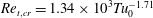 $\mathit{Re}_{t,cr}=1.34\times 10^{3}\mathit{Tu}_{0}^{-1.71}$
, where
$\mathit{Re}_{t,cr}=1.34\times 10^{3}\mathit{Tu}_{0}^{-1.71}$
, where
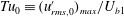 $\mathit{Tu}_{0}\equiv (u_{rms,0}^{\prime })_{max}/U_{b1}$
and can be evaluated using
$\mathit{Tu}_{0}\equiv (u_{rms,0}^{\prime })_{max}/U_{b1}$
and can be evaluated using
 $\mathit{Tu}_{0}=0.375(U_{b0}/U_{b1})(\mathit{Re}_{0})^{-0.1}$
. This can be compared with the expression for boundary layer transition,
$\mathit{Tu}_{0}=0.375(U_{b0}/U_{b1})(\mathit{Re}_{0})^{-0.1}$
. This can be compared with the expression for boundary layer transition,
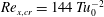 $\mathit{Re}_{x,cr}=144\,\mathit{Tu}_{0}^{-2}$
(Andersson et al.
Reference Andersson, Berggren and Henningson1999), which has been obtained from optimal growth theory and describes well experimental and DNS data of boundary layer transition. In addition, the period of the transition phase (the time between the onset of transition and the completion of it) correlates well with the critical Reynolds number. The direct correlation between
$\mathit{Re}_{x,cr}=144\,\mathit{Tu}_{0}^{-2}$
(Andersson et al.
Reference Andersson, Berggren and Henningson1999), which has been obtained from optimal growth theory and describes well experimental and DNS data of boundary layer transition. In addition, the period of the transition phase (the time between the onset of transition and the completion of it) correlates well with the critical Reynolds number. The direct correlation between
 $\mathit{Re}_{t,cr}$
and
$\mathit{Re}_{t,cr}$
and
 $\mathit{Tu}_{0}$
implies that the dominant effect of varying the initial and final Reynolds numbers is to vary the level of the FST. The initial flow, which defines the characteristics of the initial turbulence including its length scales, does not seem to have a significant effect on transition for the flow conditions examined in this study.
$\mathit{Tu}_{0}$
implies that the dominant effect of varying the initial and final Reynolds numbers is to vary the level of the FST. The initial flow, which defines the characteristics of the initial turbulence including its length scales, does not seem to have a significant effect on transition for the flow conditions examined in this study.
The high- and low-speed velocity streaks seem to play an important role in the cases where the Reynolds number ratio is relatively high, including S11, S12 and S01, but not under other flow conditions, which is suggestive that potentially different transition mechanisms are dominant in different flow transients examined herein. The minimum spanwise correlation of the streamwise velocity (
 $R_{11,min}$
) reaches a similar high peak value in the pre-transition phase in each case of the former group, and rapidly reduces during the transition. By contrast, for the cases in the latter group, the streaks remain relatively weak, albeit strengthened somewhat during the pre-transition phase, and more interestingly are only slightly weakened during the transition phase. In all the cases, the absolute value of the spacing of the streaks reduces rapidly at the beginning of the transient, but then remains largely unchanged during the most part of the pre-transition phase. This constant spacing varies from case to case, being lower with a higher initial, or a lower final, Reynolds number. The transition in terms of the generation of turbulent spots exhibits itself as intermittency in the wall-normal fluctuating velocity shown with flatness. The intermittence peaks at the time of onset of transition, and is stronger when the Reynolds number ratio is higher. For the lowest Reynolds-number-ratio case, any changes of the flatness of
$R_{11,min}$
) reaches a similar high peak value in the pre-transition phase in each case of the former group, and rapidly reduces during the transition. By contrast, for the cases in the latter group, the streaks remain relatively weak, albeit strengthened somewhat during the pre-transition phase, and more interestingly are only slightly weakened during the transition phase. In all the cases, the absolute value of the spacing of the streaks reduces rapidly at the beginning of the transient, but then remains largely unchanged during the most part of the pre-transition phase. This constant spacing varies from case to case, being lower with a higher initial, or a lower final, Reynolds number. The transition in terms of the generation of turbulent spots exhibits itself as intermittency in the wall-normal fluctuating velocity shown with flatness. The intermittence peaks at the time of onset of transition, and is stronger when the Reynolds number ratio is higher. For the lowest Reynolds-number-ratio case, any changes of the flatness of
 $v^{\prime }$
are very small and can hardly be associated with the transition.
$v^{\prime }$
are very small and can hardly be associated with the transition.
Acknowledgements
The authors gratefully acknowledge the funding from UK Engineering and Physical Science Research Council (Grant No. EP/G068925/1). This work made use of the facilities of N8 HPC provided and funded by the N8 consortium and EPSRC (Grant No. EP/K000225/1). The Centre is co-ordinated by the Universities of Leeds and Manchester.


 Open access