


Electoral platforms should reflect what voters want. Yet predicting the precise ideological preferences of the decisive voter proves challenging, even for the candidates themselves. A candidate’s ability to predict whether their decisive voter prefers left or right policies often depends on the electoral district. Candidates gain a sense of which policies their voters prefer, based on how their district leans (centrist or extreme). For example, in the United States, there is little (to no) uncertainty in any election cycle regarding whether the median voter in San Francisco, California, prefers leftist policies. But in Bury North, Greater Manchester, which is the most marginal constituency in the United Kingdom, the decisive voter’s preferred policies are harder to identify. These examples suggest that a district’s leaning reflects more than the decisive voter’s preferred policy. In particular, there is little risk in adopting extreme platforms in extreme-leaning places, whereas there is more uncertainty in centrist-leaning districts regarding whether the decisive voter’s preferred policy is to the left or right.
In this article, we show that uncertainty about the ideological position of the decisive voter, and the kind of information a district’s leaning provides, are important for understanding electoral competition. We develop a novel theory of electoral competition between two policy-motivated candidates, one whose preferred policy is on the left while the other’s is on the right. The representative voter in our model cares both about ideological policy as well as the competence of office holders, a quality independent of ideological concerns. We call the weight the voter places on competence (relative to ideology) the salience of competence. In our model, candidates choose their policy platforms while uncertain of two things. First, voters learn about the competence gap between candidates over the course of the campaign.Footnote 1 Because of this, candidates are unsure who will enjoy a nonideological advantage at the moment of choosing their campaign platforms. Second, candidates do not know their voters’ exact ideological preferences. Instead, and novel to our model, candidates only know their district’s partisan leaning, which serves as a signal of the voter’s most preferred ideological position and extreme leanings provide a more precise signal than centrist leanings.
We present three theoretical results about electoral competition and partisan leaning. Our first result shows that districts are divided endogenously into two categories which differ in what motivates campaign competition. First, electoral competition in relatively “extreme” districts is primarily driven by how much voters will learn about the competence gap between candidates. In particular, because the voter’s ideal point is relatively well known in ideologically extreme districts, candidates’ policy positions depend on potential competence differences. Second, by contrast, in relatively centrist districts, electoral competition is primarily driven by uncertainty about the location of the representative voter’s ideal point.
Our main contribution is to show that partisan leaning and the salience of competence are important drivers of platform polarization, that is, the distance between candidate platforms.Footnote 2 Our first main result shows that in centrist districts platform polarization strictly increases as the partisan leaning becomes more centrist, whereas in extreme districts polarization is driven by the competence gap and is therefore constant in leaning. Our second result shows that increasing the salience of competence increases polarization through two channels. First, increased salience of competence reduces the benefits of moderating toward the district’s partisan leaning in extreme districts, thus increasing polarization. Second, the salience of competence also influences the categorization of districts, and an increase in the salience of competence drives up the share of districts that are extreme.Footnote 3 Taken together, these two effects reinforce each other and lead to higher polarization on average.
We take our theoretical results to data from the mayoral elections of 2012, 2016, and 2020 in the 95 largest Brazilian cities—an ideal setting to evaluate our theory for three reasons. First, the timing of the COVID-19 pandemic in relation to Brazil’s electoral calendar created an exogenous shock to the salience of competence in these cities: the pre-scheduled mayoral elections of 2020 happened precisely between the first and second waves of infection. We use a combination of qualitative and quantitative evidence to first show that the competence of local candidates indeed became more salient to voters in that cycle.
Second, the ideological leaning of these large cities, measured by the national vote for the presidential candidate of the PT, is a reliable proxy for partisan leaning. The measure is historically polarized on the Left–Right dimension, stable across elections, and highly heterogeneous. Furthermore, when looking at voting data at the polling booth level, the variance of the vote distribution is higher in centrist cities than in extreme ones, as suggested by our theory.
Third, because all mayoral candidates in Brazil are required to disclose a document detailing their campaign platforms before the election, we can develop a measure of their policy positions. These campaign platforms are fairly heterogeneous, given that policy implementation in Brazil is highly decentralized, and mayors—particularly in large cities—are in charge of services such as health care, education, transportation, infrastructure, and even public security. We use several text-analysis techniques to transparently estimate platform polarization in these cities, combined with the Finanças do Brasil’s (FINBRA) dataset of local finances, which allows us to observe which policy areas concentrate most of the actual spending. In that, our polarization measure contributes to an empirical literature that has already used polarization measures based on a variety of other sources such as court decisions (Clark Reference Clark2009), roll-call voting (Poole and Rosenthal Reference Poole and Rosenthal2000), campaign contributions (Bonica Reference Bonica2013), candidate manifestos (Catalinac Reference Catalinac2018), and legislator speeches (Motolinia Reference Motolinia2021).
Our empirical findings are consistent with the theoretical results. We first present a robust empirical pattern: in elections with lower salience of competence (2012/2016), polarization is increasing in the city’s centrism, and stable across elections. We then use the exogenous timing of COVID-19 and a differences-in-differences (DiD) design to estimate the shift in polarization in 2020. We show that a shock to the salience of competence leads to an increase in polarization that is concentrated in cities with more extreme partisan leanings. These effects are not restricted to one end of the spectrum, as they apply to both Left- and Right-leaning cities.
We conclude by showing that our empirical estimates are robust to alternative specifications, highly correlated with the actual COVID-19 incidence across cities, not exclusively driven by shifts in health-related proposals, and not driven by the contemporary Rightward shift in the Brazilian electorate who elected Jair Bolsonaro president in 2018. We also consider two alternative models. In the first alternative model, partisan leaning has no influence on the variance of the signal it provides about the representative voter’s ideal point and each district receives valence shocks from a common distribution. In the second alternative model, the informativeness of partisan leaning is reversed, that is, it becomes more informative as it becomes more centrist, which is consistent with accounts where politicians learn about their decisive voter from previous election wins/losses. We show that in each of these alternative models the empirical implications about polarization do not match our empirical results. Our main model, where the precision of the signal partisan leaning provides becomes more precise as it becomes more extreme, is a better fit to the data.
RELATED LITERATURE
Our article builds on the Empirical Implications of Theoretical Models tradition in political science. We explore both comparative static implications that follow from our model, which is fairly standard in applications, as well as what our model implies about the potential sample of cases—that is, electoral districts. This allows us to consider more seriously the commensurability of our theoretical results with the empirical estimand from our design (Bueno de Mesquita and Tyson Reference Bueno de Mesquita and Tyson2020), and look for heterogeneity within the sample we study.
We build on models with policy-motivated candidates with aggregate uncertainty (Calvert Reference Calvert1985; Roemer Reference Roemer1997; Wittman Reference Wittman1983), a setting where one expects platform polarization.Footnote 4 Contrary to spatial models of electoral competition with probabilistic voting that exclusively incorporate electoral uncertainty as either purely about the location of the decisive voter (Buisseret and Van Weelden Reference Buisseret and Van Weelden2022; Sasso, Judd, and Steel Reference Sasso, Judd and Steel2024) or as a valence shock (Desai Reference DesaiForthcoming; Invernizzi Reference Invernizzi2023), our model includes both. The substantive importance of modeling uncertainty about voters in these two different ways has been highlighted by (Ashworth and Bueno de Mesquita Reference Ashworth and Bueno de Mesquita2009), who show how results can change markedly depending on the modeling choice.
The theoretical literature on polarization in political platforms has established that while beneficial in moderation, extreme polarization drives voter welfare down (Bernhardt, Duggan, and Squintani Reference Bernhardt, Duggan and Squintani2009). Others have identified mechanisms influencing platform polarization, such as economic development (Desai Reference DesaiForthcoming), electoral rule disproportionality (Matakos, Troumpounis, and Xefteris Reference Matakos, Troumpounis and Xefteris2016), foreign manipulation (Antràs and Padró i Miquel Reference Antràs and Padró i Miquel2011), and motivated reasoning in a dynamic setting (Callander and Carbajal Reference Callander and Carbajal2022). Focusing on valence, in a multidimensional setting with office-motivated candidates, a large enough valence advantage is sufficient for the existence of an equilibrium (Ansolabehere and Snyder Reference Ansolabehere and Snyder2000), and in a setting with policy-motivated candidates and electoral uncertainty, a small valence advantage leads the advantaged candidate to moderate and the disadvantaged candidate to polarize (Groseclose Reference Groseclose2001). Disentangling valence considerations from ideological considerations, however, remains a relatively understudied topic. Exceptions are Bernhardt, Câmara, and Squintani (Reference Bernhardt, Câmara and Squintani2011), who show that dynamic considerations are key to understanding the tradeoff high-valence incumbents face between using their advantage to become more extreme and compromise to hold onto office for longer, and Tolvanen, Tremewan, and Wagner (Reference Tolvanen, Tremewan and Wagner2022), who show that candidates may run on ambiguous platforms to capture extremists on both sides of the ideological spectrum. Closer to our model, Desai and Tyson (Reference Desai and TysonForthcoming) study how perceived competence advantages can drive polarization directly and indirectly. Our contribution is the introduction of the concept of partisan leaning, which provides a signal of voters’ ideological preferences to candidates and is more precise as it becomes more extreme.
Finally, our findings also contribute to an empirical literature on the relationship between polarization and the COVID-19 pandemic. This work primarily focuses on the impact of pre-existing levels of polarization, or electoral incentives, on pandemic-related policies, both in Brazil (Ajzenman, Cavalcanti, and Da Mata Reference Ajzenman, Cavalcanti and Da Mata2023; Bruce et al. Reference Bruce, Cavgias, Meloni and Remígio2022; Chauvin and Tricaud Reference Chauvin and Tricaud2024) and abroad (Milosh et al. Reference Milosh, Painter, Sonin, Van Dijcke and Wright2021; Pulejo and Querubín Reference Pulejo and Querubín2021). Our analysis departs from this literature in two significant ways. We are interested in polarization as an outcome of the COVID-19 crisis, and not as the moderator of government responses. Also, both our empirical and theoretical results apply to polarization that affects policy dimensions other than COVID-19 responses, such as spending in education or public security.
THE MODEL
We develop a model where electoral competition within a district (municipality, etc.) depends on the skill or competence of candidates as well as their ideological positions. In each district, j, there is an election between two candidates, indexed by $ i\in \{L,R\} $
, whose ideological policy preferences are represented by party ideal points,
$ i\in \{L,R\} $
, whose ideological policy preferences are represented by party ideal points, $ {y}_i $
.Footnote 5 In the first stage of the game, each candidate chooses an ideological platform, denoted by
$ {y}_i $
.Footnote 5 In the first stage of the game, each candidate chooses an ideological platform, denoted by $ {\pi}_i^{\;j} $
. Candidate i’s payoff from policy
$ {\pi}_i^{\;j} $
. Candidate i’s payoff from policy $ \pi $
is given by
$ \pi $
is given by $ -|{y}_i-\pi | $
, and we can write i’s expected payoff as
$ -|{y}_i-\pi | $
, and we can write i’s expected payoff as
 $$ \begin{array}{r}-P({L}^j\mathrm{wins}\mid {\pi}_L^{\;j},{\pi}_R^{\;j})\cdot |{y}_i-{\pi}_L^{\;j}|\\ {}\hskip0.35em -(1-P({L}^j\mathrm{wins}\mid {\pi}_L^{\;j},{\pi}_R^{\;j}))\cdot |{y}_i-{\pi}_R^{\;j}|.& \end{array} $$
Candidates are also evaluated by their performance on nonideological issues, which is captured by political competence, and denoted by $ {c}_i^{\;j} $
. Denote the competence gap in district j by
$ {c}_i^{\;j} $
. Denote the competence gap in district j by $ {\gamma}^{\;j}\equiv {c}_L^{\;j}-{c}_R^{\;j} $
, which is drawn from
$ {\gamma}^{\;j}\equiv {c}_L^{\;j}-{c}_R^{\;j} $
, which is drawn from
 $$ \begin{array}{rll}{\gamma}^{\;j}\sim U[-\psi, \psi ],& & \end{array} $$
where $ \psi $
determines the variance of the competence gap.
$ \psi $
determines the variance of the competence gap.
The electorate of district j is represented by a single representative voter (e.g., the district median voter) whose ideological preferences are characterized by an ideal point $ {z}^j $
. In the second stage of our game, the district’s representative voter sees both candidates’ platforms,
$ {z}^j $
. In the second stage of our game, the district’s representative voter sees both candidates’ platforms, $ ({\pi}_L^{\;j},{\pi}_R^{\;j}) $
, her ideal point,
$ ({\pi}_L^{\;j},{\pi}_R^{\;j}) $
, her ideal point, $ {z}^{\;j} $
, and the competence gap,
$ {z}^{\;j} $
, and the competence gap, $ {\gamma}^{\;j} $
, and chooses between candidates. The importance of competence (relative to ideology) is captured by the salience of competence,
$ {\gamma}^{\;j} $
, and chooses between candidates. The importance of competence (relative to ideology) is captured by the salience of competence, $ \alpha \in [0,1] $
. The voter’s payoff in district j, when candidate i is elected, is
$ \alpha \in [0,1] $
. The voter’s payoff in district j, when candidate i is elected, is
 $$ \begin{array}{rl}{u}_{z^{\;j}}({\pi}_i^{\;j})=-(1-\alpha )|{z}^{\;j}-{\pi}_i^{\;j}|+\alpha \hskip0.3em {c}_i^{\;j}.& \end{array} $$
The first term represents the voter’s ideological payoff, which is the distance between her ideal point, $ {z}^{\;j} $
, and the policy platform of candidate i in district j,
$ {z}^{\;j} $
, and the policy platform of candidate i in district j, $ {\pi}_i^{\;j} $
. The second term represents the competence of candidate i in district j,
$ {\pi}_i^{\;j} $
. The second term represents the competence of candidate i in district j, $ {c}_i^{\;j} $
, weighed by the salience of competence,
$ {c}_i^{\;j} $
, weighed by the salience of competence, $ \alpha $
.
$ \alpha $
.
What matters for candidates’ platform choice is what they know about their districts decisive voter at the time they must choose their platform. Novel to our model, uncertainty about the voter’s ideal point is not the same across districts. Each district is characterized by its partisan leaning, $ {\lambda}^{\;j}\in [-1,1] $
, which can be thought of as where candidates “expect” the voter to be ideologically. There is a unit mass of districts, with leanings distributed uniformly on the
$ {\lambda}^{\;j}\in [-1,1] $
, which can be thought of as where candidates “expect” the voter to be ideologically. There is a unit mass of districts, with leanings distributed uniformly on the $ [-1,1] $
interval. Within each district, there is uncertainty about the ideal point of the district’s representative voter, and district leaning acts as a signal of the voter’s true position. Specifically, for
$ [-1,1] $
interval. Within each district, there is uncertainty about the ideal point of the district’s representative voter, and district leaning acts as a signal of the voter’s true position. Specifically, for $ \delta >0 $
, when the district’s leaning is
$ \delta >0 $
, when the district’s leaning is $ {\lambda}^j $
, its representative voter’s ideal point,
$ {\lambda}^j $
, its representative voter’s ideal point, $ {z}^{\;j} $
, is drawn from a uniform distribution
$ {z}^{\;j} $
, is drawn from a uniform distribution
 $$ \begin{array}{rll}{z}^{\;j}\sim U[{\lambda}^{\;j}-(1-|{\lambda}^{\;j}|)\delta, {\lambda}^{\;j}+(1-|{\lambda}^{\;j}|)\delta ].& & \end{array} $$
Partisan leaning provides a (nonstrategic) signal of the ideological position of the decisive voter, and the parameter $ \delta $
indexes the baseline variance of that signal. Several factors could influence this variance including differences between the policy and the leaning dimensions, differential turnout rates between L and R supporters, and changes in voter preferences over time.
$ \delta $
indexes the baseline variance of that signal. Several factors could influence this variance including differences between the policy and the leaning dimensions, differential turnout rates between L and R supporters, and changes in voter preferences over time.
Partisan leaning also determines the precision of the signal it provides about ideology. In centrist districts, that is, those where $ {\lambda}^{\;j}\approx 0 $
, candidates face the most uncertainty about the ideological preferences of their district, and in extreme partisan districts, that is, those with
$ {\lambda}^{\;j}\approx 0 $
, candidates face the most uncertainty about the ideological preferences of their district, and in extreme partisan districts, that is, those with $ {\lambda}^{\;j}\approx -1 $
or
$ {\lambda}^{\;j}\approx -1 $
or $ 1 $
, candidates face the least uncertainty about the ideological preferences of their district.
$ 1 $
, candidates face the least uncertainty about the ideological preferences of their district.
To summarize, the timing is as follows: (i) candidates in district j select their policy proposals $ {\pi}_L^{\;j} $
and
$ {\pi}_L^{\;j} $
and $ {\pi}_R^{\;j} $
; (ii) the location of the decisive voter,
$ {\pi}_R^{\;j} $
; (ii) the location of the decisive voter, $ {z}^{\;j} $
, and the competence gap,
$ {z}^{\;j} $
, and the competence gap, $ {\gamma}^{\;j} $
, are realized; and (iii) the voter votes and the winning candidate’s platform is implemented.Footnote 6 We restrict attention to party ideological preferences that are more extreme than those of representative voters, that is, where
$ {\gamma}^{\;j} $
, are realized; and (iii) the voter votes and the winning candidate’s platform is implemented.Footnote 6 We restrict attention to party ideological preferences that are more extreme than those of representative voters, that is, where $ {y}_L<-1-\delta $
and
$ {y}_L<-1-\delta $
and $ {y}_R>1+\delta $
, which precludes corner solutions and simplifies the analysis.
$ {y}_R>1+\delta $
, which precludes corner solutions and simplifies the analysis.
Comments on the Model
Partisan leanings are a (nonstrategic) signal of the ideological preferences of voters, where the leaning of an electoral district, $ {\lambda}^{\;j} $
, determines both the decisive voter’s ideological preferences and the precision of the signal leaning provides about the median voter’s ideal point,
$ {\lambda}^{\;j} $
, determines both the decisive voter’s ideological preferences and the precision of the signal leaning provides about the median voter’s ideal point, $ {z}^{\;j} $
. The signal that leaning provides of the voter’s ideal point in district j has variance
$ {z}^{\;j} $
. The signal that leaning provides of the voter’s ideal point in district j has variance
 $$ \begin{array}{rl}Var({z}^{\;j})={(1-|{\lambda}^{\;j}|)}^2\cdot \frac{\delta^2}{3}.& \end{array} $$
The role of partisan leanings is illustrated in Figure 1 for $ {\lambda}^{\;j}=-1,-\frac{1}{2}, $
and
$ {\lambda}^{\;j}=-1,-\frac{1}{2}, $
and $ 0 $
, respectively, showing how there is relatively less uncertainty in a district where the voter is expected to be extreme, compared to a centrist district where the voter could be moderate or extreme.
$ 0 $
, respectively, showing how there is relatively less uncertainty in a district where the voter is expected to be extreme, compared to a centrist district where the voter could be moderate or extreme.

Figure 1. Support of $ {z}^j $
for Different Leanings
$ {z}^j $
for Different Leanings
Our model makes a specific assumption about the within-district variance of median voter’s preferences in order to capture the motivating intuition that, in centrist districts, it is harder to predict whether the decisive voter prefers leftist or rightist policies. That being said, we acknowledge that other assumptions about this variance might also be consistent with this initial intuition. For example, the uncertainty about the decisive voter’s idelogical preference between the Left and Right could be constant across districts, or even decreasing in centrism. We examine different versions of our model below where we alter the relationship between partisan leaning and the precision of the signal it provides about the decisive voter’s ideal point. We show that the role of leaning in our model is exclusively consistent with the data patterns displayed in the mayoral elections in Brazilian cities (see Figure 8) and that it better captures campaign platform polarization in the data when compared to alternative modeling choices (see section “Alternative Measures and Explanations” below).
In our model, the competence gap is not perfectly known by candidates when they choose their platforms, which in Brazil is about a month before the election. Our formulation of competence uncertainty reflects the idea that a voter’s perception of the competence gap between two candidates is not known precisely at the moment candidates choose electoral platforms, and it can fluctuate over the course of the campaign. There are at least two reasons why the competence gap is learned over the course of an electoral campaign, rather than being known ex ante and fixed throughout the campaign. First, events such as gaffes or scandals often influence voters’ perceptions of candidates (Di Lonardo Reference Di Lonardo2017). Second, aspects of candidates, especially challengers, are revealed through the course of a campaign, and thus influence what aspects of competence are relevant to voters on election day. Take, for example, João Dória, who was elected mayor of São Paulo in 2016. Early on in the campaign period in late August, only 7% of the electorate declared their intentions to vote for him. But during the campaign period, his career as a businessman earned him a reputation for being a competent manager, with him eventually winning the race in early October.
We assume that neither L nor R enjoys a competence advantage on average to ensure that our theoretical results come from the interaction of uncertainty about competence advantages, which resemble valence, and uncertainty about local ideological preferences that vary across districts, which is novel to our setup. Large competence advantages, relative to the general pool of challengers, tend to create a scare-off effect among potential challengers (e.g., Cox and Katz Reference Cox and Katz1996), implying that in contested elections there may be reason to believe that challengers are not systematically disadvantaged at the entry stage (Alexander Reference Alexander2021). Our assumption would be a problem in our empirical specification if partisan leaning were correlated with factors that might indicate an early insurmountable competence advantage.Footnote 7
Finally, our model presents a stylized election where candidates are evaluated along two dimensions, ideology and competence, by a single representative voter. Our model isolates the role of the district’s leaning as a signal of the voter’s ideological preferences. We intentionally omit a number of other features of elections that, although important, are not critical to the mechanism here. We focus our theory on the role of district leaning in isolation, as though we are holding such factors fixed, as in an experiment (Paine and Tyson Reference Paine, Tyson, Berg-Schlosser, Badie and Morlino2020).
PLATFORMS AND POLARIZATION
We suppress district index, j, whenever possible to simplify exposition.Footnote 8 We start with the representative voter (in the second stage) who knows her ideal point, z, the competence gap, $ \gamma $
, and candidates’ platforms,
$ \gamma $
, and candidates’ platforms, $ ({\pi}_L,{\pi}_R) $
. From Equation 2, the voter chooses L if and only if
$ ({\pi}_L,{\pi}_R) $
. From Equation 2, the voter chooses L if and only if
 $$ \begin{array}{rll}-(1-\alpha )|z-{\pi}_L|+\alpha \hskip0.3em {c}_L\ge -(1-\alpha )|z-{\pi}_R|+\alpha \hskip0.3em {c}_R,& & \end{array} $$
and chooses R otherwise. Rearranging, the voter’s decision rule is a cutoff,
 $$ \begin{array}{rll}{\gamma}^{*}({\pi}_L,{\pi}_R;z)=\frac{1-\alpha }{\alpha }(|z-{\pi}_L|-|z-{\pi}_R|),& & \end{array} $$
where the representative voter votes for L if and only if $ \gamma \ge {\gamma}^{*}({\pi}_L,{\pi}_R;z) $
and votes for R otherwise. The cutoff rule,
$ \gamma \ge {\gamma}^{*}({\pi}_L,{\pi}_R;z) $
and votes for R otherwise. The cutoff rule, $ {\gamma}^{*}({\pi}_L,{\pi}_R;z) $
, determines the level of the competence gap,
$ {\gamma}^{*}({\pi}_L,{\pi}_R;z) $
, determines the level of the competence gap, $ \gamma $
, for which the voter prefers L to R, and its value depends on candidates’ platform choices,
$ \gamma $
, for which the voter prefers L to R, and its value depends on candidates’ platform choices, $ {\pi}_L $
and
$ {\pi}_L $
and $ {\pi}_R $
, as well as the voter’s true ideal point, z.
$ {\pi}_R $
, as well as the voter’s true ideal point, z.
Moving backward to the candidates, when they choose their ideological platforms, they do not know the voter’s ideal point, z, nor the competence gap, $ \gamma $
. Consequently, candidates do not know the voter’s decision rule,
$ \gamma $
. Consequently, candidates do not know the voter’s decision rule, $ {\gamma}^{*}({\pi}_L,{\pi}_R;z) $
. Thus, the probability that L wins the election is
$ {\gamma}^{*}({\pi}_L,{\pi}_R;z) $
. Thus, the probability that L wins the election is $ P(\gamma \ge {\gamma}^{*}({\pi}_L,{\pi}_R;z)) $
, and the probability R wins is
$ P(\gamma \ge {\gamma}^{*}({\pi}_L,{\pi}_R;z)) $
, and the probability R wins is $ P(\gamma <{\gamma}^{*}({\pi}_L,{\pi}_R;z)) $
, and the problem for candidate
$ P(\gamma <{\gamma}^{*}({\pi}_L,{\pi}_R;z)) $
, and the problem for candidate $ i\in \{L,R\} $
is
$ i\in \{L,R\} $
is
 $$ \begin{array}{r}\underset{\pi_i}{\max }-P(\gamma \ge {\gamma}^{*}({\pi}_L,{\pi}_R;z)\mid \lambda )|{y}_i-{\pi}_L|\\ {}-(1-P(\gamma \ge {\gamma}^{*}({\pi}_L,{\pi}_R;z)\mid \lambda ))|{y}_i-{\pi}_R|.& \end{array} $$
A pair of ideological platforms $ ({\pi}_L,{\pi}_R) $
that simultaneously solve Equation 4 for L and R, along with
$ ({\pi}_L,{\pi}_R) $
that simultaneously solve Equation 4 for L and R, along with $ {\gamma}^{*}({\pi}_L,{\pi}_R;z) $
from above, together constitute a subgame perfect Nash equilibrium to our game. We characterize symmetric equilibrium platforms, meaning platforms that are equidistant from the district’s partisan leaning,
$ {\gamma}^{*}({\pi}_L,{\pi}_R;z) $
from above, together constitute a subgame perfect Nash equilibrium to our game. We characterize symmetric equilibrium platforms, meaning platforms that are equidistant from the district’s partisan leaning, $ \lambda $
.
$ \lambda $
.
Proposition 1. There exists a unique symmetric subgame perfect Nash equilibrium where for an extreme-left (extreme-right) district, that is, for all $ \lambda <{\overline{\lambda}}_L $
(
$ \lambda <{\overline{\lambda}}_L $
( $ \lambda >{\overline{\lambda}}_R $
),
$ \lambda >{\overline{\lambda}}_R $
),
 $$ \begin{array}{rl}\begin{array}{rll}{\pi}_L^{*}=& \hskip-0.6em \lambda -\frac{\alpha \psi }{2(1-\alpha )}\ \mathrm{and}\ {\pi}_R^{*}=& \hskip-0.6em \lambda +\frac{\alpha \psi }{2(1-\alpha )};\end{array}& \end{array} $$
for all centrist districts, that is, $ {\overline{\lambda}}_L\le \lambda \le {\overline{\lambda}}_R $
,
$ {\overline{\lambda}}_L\le \lambda \le {\overline{\lambda}}_R $
,
 $$ \begin{array}{rl}\begin{array}{rll}{\pi}_L^{\dagger }=& \hskip-0.6em \lambda -(1-|\lambda |)\delta\ \mathrm{and}\ {\pi}_R^{\dagger }=& \hskip-0.6em \lambda +(1-|\lambda |)\delta; \end{array}& \end{array} $$
and where
 $$ {\displaystyle \begin{array}{l}{\overline{\lambda}}_L=\min \left\{\frac{\alpha \hskip0.3em \psi }{2\left(1-\alpha \right)\delta }-1,0\right\}\hskip1em \mathrm{and}\\ {}{\overline{\lambda}}_R=\max \left\{1-\frac{\alpha \hskip0.3em \psi }{2\left(1-\alpha \right)\delta },0\right\}.\end{array}} $$
Proposition 1 shows that there are two qualitatively different kinds of equilibria, depending on a district’s leaning. At the time candidates choose platforms, their choices are motivated by uncertainty about the ideal point of the representative voter, z, the magnitude of which depends on the district’s leaning, $ |\lambda | $
, and uncertainty about the competence gap,
$ |\lambda | $
, and uncertainty about the competence gap, $ \gamma $
, which is substantively more important in districts that have more extreme leanings because the voter’s ideal point is relatively certain. Whichever kind of uncertainty is most salient determines the platform choices of candidates, and consequently the equilibrium level of polarization.
$ \gamma $
, which is substantively more important in districts that have more extreme leanings because the voter’s ideal point is relatively certain. Whichever kind of uncertainty is most salient determines the platform choices of candidates, and consequently the equilibrium level of polarization.
Both candidates chase the expected decisive voter, $ \lambda $
, and polarize away from
$ \lambda $
, and polarize away from $ \lambda $
based on the competence gap in extreme districts, and the leaning signal in centrist districts. From Equation 5, the equilibrium platforms in extreme districts are equidistant from the leaning
$ \lambda $
based on the competence gap in extreme districts, and the leaning signal in centrist districts. From Equation 5, the equilibrium platforms in extreme districts are equidistant from the leaning $ \lambda $
, and what drives differences in platforms between L and R is uncertainty about the competence gap.Footnote 9 Figure 2 illustrates the relationship between partisan leaning and platform choices.
$ \lambda $
, and what drives differences in platforms between L and R is uncertainty about the competence gap.Footnote 9 Figure 2 illustrates the relationship between partisan leaning and platform choices.

Figure 2. Equilibrium Platforms and Leaning
Note: This figure illustrates the equilibrium platforms for leftist leanings, i.e., for $ \lambda <0 $
. Both platforms
$ \lambda <0 $
. Both platforms $ {\pi}_L $
and
$ {\pi}_L $
and $ {\pi}_R $
follow the expected decisive voter,
$ {\pi}_R $
follow the expected decisive voter, $ \lambda $
. In extreme districts, i.e., where
$ \lambda $
. In extreme districts, i.e., where $ \lambda <{\overline{\lambda}}_L $
, platforms are expressed as in Equation 5, and in centrist districts, i.e., where
$ \lambda \ge {\overline{\lambda}}_L $
, platforms are expressed as in Equation 6. Equilibrium platforms for
$ \lambda <{\overline{\lambda}}_L $
, platforms are expressed as in Equation 5, and in centrist districts, i.e., where
$ \lambda \ge {\overline{\lambda}}_L $
, platforms are expressed as in Equation 6. Equilibrium platforms for $ \lambda >0 $
are essentially a reflection across the y-axis.
$ \lambda >0 $
are essentially a reflection across the y-axis.
Polarization—the distance between platforms—in extreme districts is
 $$ \begin{array}{rll}{\pi}_R^{*}-{\pi}_L^{*}=\frac{\alpha \psi }{1-\alpha },& & \end{array} $$
which is strictly increasing in the salience of competence, $ \alpha $
. As a district becomes more centrist-leaning, that is, as
$ \alpha $
. As a district becomes more centrist-leaning, that is, as $ -|\lambda | $
increases, then uncertainty about the voter’s ideal point becomes more important, and eventually drives candidate platform choices. In centrist districts, from Equation 6, polarization is
$ -|\lambda | $
increases, then uncertainty about the voter’s ideal point becomes more important, and eventually drives candidate platform choices. In centrist districts, from Equation 6, polarization is
 $$ \begin{array}{rll}{\pi}_R^{\dagger }-{\pi}_L^{\dagger }=2(1-|\lambda |)\delta, & & \end{array} $$
which is independent of the salience of competence, $ \alpha $
.
$ \alpha $
.
We now consider the relationship between polarization and leaning followed by the relationship between the salience of competence and polarization.
Proposition 2. Platform polarization in centrist districts is strictly increasing in the ideological centrism of the leaning, measured by $ -|\lambda | $
, whereas there is no relationship between platform polarization and district leaning in extreme districts.
$ -|\lambda | $
, whereas there is no relationship between platform polarization and district leaning in extreme districts.
Platforms move parallel to each other in $ \lambda $
as long as the district is extreme enough, and move further away from each other in
$ \lambda $
as long as the district is extreme enough, and move further away from each other in $ \lambda $
as the district leans more to the center. Proposition 2 shows that there is a positive relationship between ideological centrism (measured by district leaning) and platform polarization—but only in centrist districts. In extreme districts, where information regarding the ideological preferences of the voter is more precise, there is no relationship between polarization and leaning, because electoral competition is driven by voters’ perceptions of competence, rather than the location of the decisive voter.
$ \lambda $
as the district leans more to the center. Proposition 2 shows that there is a positive relationship between ideological centrism (measured by district leaning) and platform polarization—but only in centrist districts. In extreme districts, where information regarding the ideological preferences of the voter is more precise, there is no relationship between polarization and leaning, because electoral competition is driven by voters’ perceptions of competence, rather than the location of the decisive voter.
Proposition 2 contrasts platform polarization in a single district, as a function of that district’s leaning (all-else-equal). While we would like to directly assess Proposition 2, which is at the district level, to achieve the counterfactual comparison it outlines, we would need to observe (or identify separately) different leanings for that district. To assess how our model speaks to the data, it is important that we understand how changes in the salience of competence, $ \alpha $
, influence polarization,
$ \alpha $
, influence polarization, $ {\pi}_R-{\pi}_L $
, when averaged across all districts. We focus on the average level of polarization across districts,Footnote 10
$ {\pi}_R-{\pi}_L $
, when averaged across all districts. We focus on the average level of polarization across districts,Footnote 10
 $$ \begin{array}{l}P({\lambda}^j<{\overline{\lambda}}_L\hskip2.77695pt \mathrm{or}\hskip2.77695pt {\lambda}^j>{\overline{\lambda}}_R)({\pi}_R^{*}-{\pi}_L^{*})\\ {}+P({\overline{\lambda}}_L\le {\lambda}^j\le {\overline{\lambda}}_R)\unicode{x1D53C}[{\pi}_R^{\dagger }-{\pi}_L^{\dagger }|{\overline{\lambda}}_L\le {\lambda}^{\;j}\le {\overline{\lambda}}_R],& \end{array} $$
because any empirical estimand will measure this quantity. The first term is the level of polarization in extreme districts, and the second term is the level of polarization in centrist districts, both weighted by the prevalence of the type of district in the population.
Proposition 3. The average level of polarization across districts is strictly increasing in the salience of competence, $ \alpha $
. In particular, the level of polarization in extreme districts,
$ \alpha $
. In particular, the level of polarization in extreme districts, $ {\pi}_R^{*}-{\pi}_L^{*} $
, is strictly increasing in
$ {\pi}_R^{*}-{\pi}_L^{*} $
, is strictly increasing in $ \alpha $
, whereas the level of polarization in centrist districts,
$ \alpha $
, whereas the level of polarization in centrist districts, $ {\pi}_R^{\dagger }-{\pi}_L^{\dagger } $
, is constant in
$ {\pi}_R^{\dagger }-{\pi}_L^{\dagger } $
, is constant in $ \alpha $
. Moreover, the share of centrist districts decreases in
$ \alpha $
. Moreover, the share of centrist districts decreases in $ \alpha $
.
$ \alpha $
.
This result is about how the salience of competence influences polarization. In centrist districts, an increase in $ \alpha $
has no effect on candidate platforms, and hence no direct effect on polarization. In extreme districts, uncertainty about the competence gap influences the level of polarization, which is strictly increasing in the salience of competence,
$ \alpha $
has no effect on candidate platforms, and hence no direct effect on polarization. In extreme districts, uncertainty about the competence gap influences the level of polarization, which is strictly increasing in the salience of competence, $ \alpha $
. These two effects, which differ depending on a district’s leaning, capture the intensive margin by which the salience of competence influences the average level of polarization. The magnitude of this intensive margin is
$ \alpha $
. These two effects, which differ depending on a district’s leaning, capture the intensive margin by which the salience of competence influences the average level of polarization. The magnitude of this intensive margin is
 $$ \begin{array}{rl}\left|\right.\frac{d{\pi}_R^{*}-{\pi}_L^{*}}{d\alpha}\left|\right.=\frac{\psi }{{(1-\alpha )}^2}>0,& \end{array} $$
in extreme districts and
 $$ \begin{array}{rl}\left|\right.\frac{d{\pi}_R^{\dagger }-{\pi}_L^{\dagger }}{d\alpha}\left|\right.=0,& \end{array} $$
in centrist districts. Combining Equation 9 with Equation 10 shows that changes in polarization due to changes in the salience of competence are driven by extreme districts.
Since a shock to the salience of competence influences polarization only in extreme districts, and because whether a district is extreme is endogenous, we must also consider what determines whether a district is centrist. This amounts to analyzing, from Proposition 1, the cutoffs $ {\overline{\lambda}}_L $
and
$ {\overline{\lambda}}_L $
and $ {\overline{\lambda}}_R $
which determine the share of extreme districts, and are themselves dependent on the salience of competence,
$ {\overline{\lambda}}_R $
which determine the share of extreme districts, and are themselves dependent on the salience of competence, $ \alpha $
. In particular, using that district leanings are uniformly distributed, and that
$ \alpha $
. In particular, using that district leanings are uniformly distributed, and that $ {\overline{\lambda}}_L=-{\overline{\lambda}}_R $
, we can rewrite Equation 8 as
$ {\overline{\lambda}}_L=-{\overline{\lambda}}_R $
, we can rewrite Equation 8 as
 $$ \begin{array}{rll}\left(\right.1+{\overline{\lambda}}_L\left)\right.\left(\right.\frac{\alpha \psi }{1-\alpha}\left)\right.+2\delta {\int}_{{\overline{\lambda}}_L}^0\left(\right.1+{\lambda}^j\left)\right.\hskip0.2em d{\lambda}^j.& & \end{array} $$
This expression highlights that the salience of competence, $ \alpha $
, also influences the share of districts where polarization depends on the salience of competence, identifying the extensive margin by which the salience of competence influences polarization. In particular,
$ \alpha $
, also influences the share of districts where polarization depends on the salience of competence, identifying the extensive margin by which the salience of competence influences polarization. In particular, $ {\overline{\lambda}}_L $
is strictly increasing in
$ {\overline{\lambda}}_L $
is strictly increasing in $ \alpha $
, while
$ \alpha $
, while $ {\overline{\lambda}}_R $
is strictly decreasing in
$ {\overline{\lambda}}_R $
is strictly decreasing in $ \alpha $
, establishing that an increase in the salience of competence reduces the number of centrist districts, by a magnitude of
$ \alpha $
, establishing that an increase in the salience of competence reduces the number of centrist districts, by a magnitude of
 $$ \begin{array}{rll}\left|\right.\frac{d{\overline{\lambda}}_i}{d\alpha}\left|\right.=\frac{\psi }{2{(1-\alpha )}^2\delta }.& & \end{array} $$
This latter effect further increases the observed level of polarization when averaging over districts because an increase in $ \alpha $
implies that more districts are extreme.
$ \alpha $
implies that more districts are extreme.
In sum, the overall effect of the salience of competence, $ \alpha $
, on the average level of polarization can be decomposed into two reinforcing channels: an intensive and extensive margin. When taken together, these show that polarization increases as the salience of competence increases.
$ \alpha $
, on the average level of polarization can be decomposed into two reinforcing channels: an intensive and extensive margin. When taken together, these show that polarization increases as the salience of competence increases.
Finally, while partisan leaning and its heterogeneous informativeness are our primary contributions, partisan leaning interacts with uncertainty regarding the competence gap, especially for the result in Proposition 3. To see this more clearly, consider taking $ \psi \to 0 $
. In extreme districts, both candidates’ platforms converge to the district leaning, eliminating platform polarization—a “median voter theorem”-style logic. Additionally, the cutoffs
$ \psi \to 0 $
. In extreme districts, both candidates’ platforms converge to the district leaning, eliminating platform polarization—a “median voter theorem”-style logic. Additionally, the cutoffs $ {\overline{\lambda}}_L $
and
$ {\overline{\lambda}}_L $
and $ {\overline{\lambda}}_R $
approach the endpoints of the space of partisan leanings,
$ {\overline{\lambda}}_R $
approach the endpoints of the space of partisan leanings, $ -1 $
and
$ -1 $
and $ 1 $
, respectively, and as a consequence, removing uncertainty about the competence gap makes all districts “centrist” districts where polarization does not depend on the salience of competence. More precisely, if there is no uncertainty regarding the competence gap, then
$ 1 $
, respectively, and as a consequence, removing uncertainty about the competence gap makes all districts “centrist” districts where polarization does not depend on the salience of competence. More precisely, if there is no uncertainty regarding the competence gap, then $ \alpha $
has no effect on platforms.
$ \alpha $
has no effect on platforms.
Before proceeding to the empirical application, we briefly summarize the two main theoretical results from Propositions 2 and 3 that we take to the data, which are also illustrated in Figure 3. First, Proposition 2 shows that if the salience of competence ( $ \alpha $
) is low enough, polarization is always increasing in centrism
across districts (municipalities). When
$ \alpha $
) is low enough, polarization is always increasing in centrism
across districts (municipalities). When $ \alpha $
is low enough, there is a strong positive relationship between polarization and centrism, measured by
$ \alpha $
is low enough, there is a strong positive relationship between polarization and centrism, measured by $ -|\lambda | $
. Second, Proposition 3 establishes that an increase in the salience of competence attenuates the leaning–polarization relationship across municipalities. The increase in average polarization, therefore, stems from districts that are extreme.
$ -|\lambda | $
. Second, Proposition 3 establishes that an increase in the salience of competence attenuates the leaning–polarization relationship across municipalities. The increase in average polarization, therefore, stems from districts that are extreme.

Figure 3. District Centrism and Equilibrium Polarization
Note: This figure illustrates the two theoretical implications we take to the data. $ {\overline{\lambda}}_{low} $
and
$ {\overline{\lambda}}_{low} $
and $ {\overline{\lambda}}_{high} $
denote the cutoffs that determine whether a district is extreme or centrist when
$ {\overline{\lambda}}_{high} $
denote the cutoffs that determine whether a district is extreme or centrist when $ \alpha $
is low or high, respectively. When
$ \alpha $
is low or high, respectively. When $ \alpha $
is low, there is a strong positive relationship between the centrism of the district,
$ \alpha $
is low, there is a strong positive relationship between the centrism of the district, $ -|\lambda | $
, and polarization. As
$ -|\lambda | $
, and polarization. As $ \alpha $
becomes high, the share of extreme districts increases, the positive relationship between polarization and
$ \alpha $
becomes high, the share of extreme districts increases, the positive relationship between polarization and $ -|\lambda | $
attenuates, and average polarization increases, with the increase concentrated in extreme districts.
$ -|\lambda | $
attenuates, and average polarization increases, with the increase concentrated in extreme districts.
A CASE STUDY IN BRAZILIAN MUNICIPALITIES
We first provide a brief background on features of Brazilian politics that are relevant to our empirical application. We then provide details on how we measure—in Brazilian cities—the following empirical quantities that are pertinent to our theory: local partisan leaning, platform polarization, and the shock to the salience of competence in mayoral elections. We then proceed to the empirical estimation and discussion of the results.
Two main features of the Brazilian party system make it a suitable empirical application for our theory. Our model is set in a political environment where leaning in the Left–Right dimension is relevant for electoral competition, widely recognized by voters and politicians, stable over time, and interpretable on similar scale across districts. While Brazil has a fragmented party system, with 30+ active parties, the coarse Left–Right party divide is highly salient (Power and Zucco Reference Power and Zucco2009; Reference Power and Zucco2012). Party positioning on this divide is consistent across surveys with legislators, experts, and voters (Desai and Frey Reference Desai and Frey2023), and even with roll-call votes in Congress.Footnote 11 At least for the period of our empirical analysis, Left–Right positioning is also aligned with preferences for redistribution for both politicians (Power and Zucco Reference Power and Zucco2012) and voters (Hunter and Power Reference Hunter and Power2007; Lupu Reference Lupu, Levitsky, Loxton, Dyck and Dominguez2016). More importantly, the divide has defined the presidential vote since the democratization with PT (Worker’s Party) on the Left, and on the right, PSDB in 1994–2014 and Jair Bolsonaro (PSL) in 2018 and 2022. This is partly due to PT’s institutional stability, which anchors both the ideological space from the Left and the competition with the more decentralized Right (Samuels and Zucco Reference Samuels and Zucco2018).
Our model also assumes that candidates adapt policies to the preferences of the decisive voter in each city. In other words, we need Right-wing parties to be able to credibly move local policies Left, and vice versa. Here, both the ideological flexibility and regional fragmentation of Brazilian parties help bridge the theory to the data. Despite the well-established Left–Right cleavage described above, it is much harder to ideologically differentiate parties within the same broad group. Particularly for some large center-Right parties, they are often better described by their modus operandi (e.g., clientelism) or rent-seeking behavior (e.g., some consistently engage in alliances with Leftist incumbents) rather than ideological coherence (Power and Rodrigues-Silveira Reference Power and Rodrigues-Silveira2019). Also, parties struggle to control individual politicians (Desposato Reference Desposato2006; Klašnja and Titiunik Reference Klašnja and Titiunik2017), and local candidates have ample flexibility to tailor their platforms to local electorates. For example, Rightist mayors often prioritize redistribution in poor areas (Desai and Frey Reference Desai and Frey2023), and even PT’s governor of Bahia recently became tough on crime.Footnote 12 Altogether, the solidity of the nationally recognized Left–Right cleavage anchored around PT, combined with the flexibility for local candidates coming from the party fragmentation, makes Brazil a suitable environment to study our theory.
Our application focuses on mayoral elections in the 95 largest Brazilian cities—those that have a runoff system—in 2012, 2016, and 2020.Footnote 13 These races constitute the ideal group for our analysis, for two reasons. First, voters are more exposed to the campaign platforms of the top candidates in large Brazilian municipalities, both in time and intensity. Not only does the potential runoff often extend campaign times for the top candidates, but they also have subsidized, mandatory, prime-time TV campaigns on all the over-the-air channels.Footnote 14 Second, given the highly decentralized structure of public spending, mayors of large cities spend the budget on a broad portfolio of policy areas such as health care, education, social assistance, transportation, and even public security.
A Proxy for Ideological Leaning at the Municipal Level
Our empirical proxy for partisan leaning is based (without loss of generality) on the share of the municipal vote for the Left (e.g., Workers Party, PT) in the final round of the last pre-treatment presidential election in Brazil (2010), which we denote by $ Lef{t}_{\;j} $
in municipality j. Specifically, in municipality j, leaning is given by
$ Lef{t}_{\;j} $
in municipality j. Specifically, in municipality j, leaning is given by
 $$ \begin{array}{rll}ln{g}_{\;j}=1/2-|Lef{t}_{\;j}-1/2|.& & \end{array} $$
Leaning is defined in the interval $ [0,1/2] $
, and that more extreme cities—either to the Left or Right—have lower values.
$ [0,1/2] $
, and that more extreme cities—either to the Left or Right—have lower values.
The rationale behind our choice is threefold. First, Brazilian presidential races are historically highly polarized in the Left–Right dimension: all elections since democratization were dominated by one Left- and one Right-wing party.Footnote 15 Second, the share of Left-wing presidential votes in each municipality is persistent across elections, and highly heterogeneous across municipalities. The average PT vote share in 2010 was 53%, with values ranging from 24% to 84%. Supplementary Figure D.1 also shows that the 2010 vote shares are highly correlated—across municipalities—with the shares in the subsequent presidential races of 2014 and 2018.
Third, at the core of our theory is the idea that the uncertainty about the ideological preference of the decisive voter is positively correlated with district centrality. Figure 4 shows that this relationship holds for our leaning measure. For each city in the sample, we calculate the variance of PT’s vote share in 2010, based on voting data at the ballot box level (e.g., São Paulo has 90,446 ballot boxes, with slightly more than 300 votes each, on average). We then compare these municipality-level variances to the leaning measure. The plot shows that the variance is lower in extreme cities, and higher in more centrist locations.

Figure 4. Variance of PT’s Vote Share in 2010 at the Ballot Box Level
Note: The 95 cities in the sample are aggregated in 20 bins along the x-axis. The values in the y-axis have the average variance for each bin. Variances are calculated for each city with PT’s vote share in 2010 at the ballot box level. The line shows a quadratic fit.
Measuring Platform Polarization
We measure platform polarization using data about the policy proposals of mayoral candidates in the 95 largest Brazilian cities. Since 2009, all candidates for executive offices are required by the federal electoral court (TSE) to disclose a document with their campaign platforms and priorities. These documents typically have extended discussions on the candidates’ proposals for different areas of the local administration, and are published in the TSE’s website around a month before the election (TSE 2012–2020). They are also extensively scrutinized by the local press.Footnote 16
We use the TSE documents to identify and measure the policy priorities, in six different areas, of the two top contenders in each election. The relevance of policy areas is based on the classification of the actual budget expenses of Brazilian cities, obtained from the FINBRA database maintained by the National Treasury (STN 2013–2020; 2009–2012). Figure 5 shows the main spending categories in these 95 cities, according to this classification. Note that, although these 10 categories account for 99% of all policy-related expenditures,Footnote 17 only six of them—health care, education, transportation/urbanization, sanitation/the environment, social assistance, and public security—individually account for more than 1% of local budgets. We show in Supplementary Table C.4 that our results are robust to the inclusion of the other four minor categories.

Figure 5. Spending Categories in Large Brazilian Cities
Note: Spending is from 2017 to 2020. For correspondence, the word frequency shown here only includes the proposals in the same electoral cycle (2016). The light gray columns show the average share of each category (99% of total expenses). The dark gray columns show the share of policy-related words in candidates’ platforms that belong to each of the six main categories—using the first two words shown in Table 1, for each category. HEAL = Health care; EDUC = Education; TRAN = Transportation and Urbanization; SANI = Sanitation and the Environment; SOCI = Social Assistance; PSEC = Public Security; CULT = Culture; SPOR = Sports and Leisure; HOUS = Housing; and BUSI = Businesses and Tourism.
Our primary measure of polarization is built using the frequency of words that are uniquely and directly related to each policy area. More precisely, we first find the two most frequent policy words for each category in all documents. We then calculate the score of each policy category as the count of its policy words as a share of the total frequency of all policy words in the document. We use these scores to calculate the polarization level in each city-year, which is the six-dimensional Euclidean distance between the proposals of the top two candidates.
The most common policy-related terms in each category are shown in Table 1, and the full list of the 200 most frequent words in the sample is shown in Supplementary Table B.2. Figure 5 has the relative frequencies of these categories in the candidates’ platforms (dark gray columns), and how they are largely consistent with the actual budget implementation. In the Supplementary Material, we show that the results are robust to several different choices in the number of words used to define the categories. Supplementary Table C.6 shows the estimates for measures built with the three and four most frequent words for each category, respectively. Supplementary Table C.7 has estimates for measures that use all policy words in each category that are among the 200 or 300 most frequent words in the sample, respectively. Supplementary Table B.3 details which words are used in each specification.
Table 1. Main Words in Each Budget Category

Note: Supplementary Table B.2 has the list of the 200 most frequent words in the sample. The only exception here is the word sanitation, which is the 244th more frequent in the sample, and 5th in the category (see Supplementary Table B.3). It is included here because it is the category title.
As an illustration, consider the city of Cariacica (ES), where the 2020 race was a runoff between candidates from DEM (Right-wing) and PT (Left-wing). DEM’s candidate emphasized his proposals for public security, highlighting that the area would be “one of the priorities of this administration.”Footnote 18 The document explains in detail the several action points for this area such as arming the municipal guard, hiring officers, and increasing neighborhood patrols. Overall, the share of policy terms in the document that were dedicated to security measures was 29%. The same share for the proposal of PT’s candidate was only 9%. Not only did the Left-wing’s document fail to single out security as a priority, but it also had a shorter discussion on the topic that was primarily focused on investing in education and leisure for youth populations.Footnote 19
Our primary metric has a number of advantages for our empirical exercise. First, simple metrics are highly intuitive (Eggers and Spirling Reference Eggers and Spirling2018), easy to interpret, and also have the virtue of ensuring “transparency and replicability” (Wilkerson and Casas Reference Wilkerson and Casas2017). Another important advantage is that simple metrics can be explicitly linked to theoretical objects or out-of-sample topic categorizations such as the structure of local budgets that we use here.
Our simple metric, however, raises two main concerns. The first is that, by relying on the frequency of a few selected terms, it might fail to capture polarization that comes from the remaining words in the document. Second, a metric that is free from assumptions about the ideology of parties and/or policies might not be substantively related to our empirical proxy for partisan leaning described above. To address such concerns, we first show that cities with similar leaning have, on average, candidates that propose similar policies (Supplementary Figure D.3). This suggests that leaning is highly correlated with the content of the average campaign platforms across cities and that it does so without additional assumptions about the ideological content of specific policy categories.
We also replicate our analysis using the well-known scaling approach based on Wordscores (Laver, Benoit, and Garry Reference Laver, Benoit and Garry2003), which has been previously used to study the Brazilian proposals data (Pereira Reference Pereira2021). Here, we follow Desai and Frey (Reference Desai and Frey2023) and categorize the largest parties in 2012 as either Left- or Right-wing. We then use the proposals of their 2012 mayoral candidates to train the algorithm that classifies the whole set of documents on a Left–Right scale,Footnote 20 and use the absolute distance between the scores of the top two candidates as a measure of polarization.
Including the results based on the Wordscores metric side-by-side with our main specification provides a few advantages. First, this alternative metric uses assumptions on the ideological leaning of parties, but it does not rely on assumptions about the relevance of policy categories in local budgets. In doing so, it provides evidence that our main findings are not an artifact of our polarization metric. They are also more naturally interpretable in the same dimension as our leaning variable. The striking similarity between leaning and polarization across these two metrics (as later shown in Table 2) provides additional evidence that our primary policy-based metric has substantive meaning in the Left–Right dimension of leaning.
Table 2. Polarization of Mayoral Campaigns during the Pandemic

Note: A total of 256 observations in all regressions. The coefficients come from Equation 11. The outcomes were normalized to values between zero and one for better comparison between metrics. All covariates are described in Footnote footnote 25. City covariates are measured pretreatment and become redundant with Municipality fixed effects. The same happens to $ {\beta}_2 $
and
$ {\beta}_2 $
and $ {\beta}_1 $
(with year FEs). The full regression coefficients are shown in Supplementary Tables C.1 (policy words) and Table C.2 (wordscores).
$ {\beta}_1 $
(with year FEs). The full regression coefficients are shown in Supplementary Tables C.1 (policy words) and Table C.2 (wordscores). $ {}^{+}p<0.1 $
,
$ {}^{+}p<0.1 $
, $ {}^{*}p<0.05 $
.
$ {}^{*}p<0.05 $
.
Finally, the party-based metric produces scores for each proposal that are based on the frequency of all words in the documents, rather than policy words only, which addresses the concerns with the simplicity of our measure.
In the Supplementary Material, we show results estimated with an additional alternative measure of polarization that is built using the seeded sequential topic model by Watanabe and Baturo (Reference Watanabe and Baturo2024). This is a semi-supervised approach that has the computational advantages of traditional topic models, with the use of seed words as a weak form of supervision on the definition of topics. In a nutshell, regular LDA-based topic models split documents in a prespecified number of topics based on the relative clustering of words in the documents. This approach reweights the clusters of words based on their relationship with seed words provided by the researcher, and by doing so creates topics that are more likely to be substantively related to the (seed) themes defined by the researcher. We fit six topics on the data using the words in Table 1 as seed. In Supplementary Appendix B, we provide additional details on the construction of these databases, which also include details on the standard preprocessing steps.
COVID-19: A Shock to the Salience of Competence
In a context where voters value both ideology and competence, we are interested in the impact of the “shock” introduced by the unprecedented and quick spread of COVID-19 in 2020. We argue that one of the most prominent impacts of the pandemic is that it altered the importance voters place on nonideological aspects of politicians, especially competence. In our model, the parameter $ \alpha $
captures the salience to voters of such a shock. In the data, the (prescheduled) timing of the 2020 local elections in Brazil, combined with the country’s decentralized system of public health spending, creates an ideal context that helps us study the relationship between the salience of competence and platform polarization.
$ \alpha $
captures the salience to voters of such a shock. In the data, the (prescheduled) timing of the 2020 local elections in Brazil, combined with the country’s decentralized system of public health spending, creates an ideal context that helps us study the relationship between the salience of competence and platform polarization.
The country-wide mayoral elections happened nearly 8 months into the pandemic, between the first and second waves of infection. This event increased the salience of the mayor’s managerial ability not only due to its timing, but also because municipal administrations in Brazil bear the bulk of the responsibility of delivering health care services through the universal system (SUS). Health care services are the largest budget category in municipalities, and also the highest priority for voters: in a 2020 survey, 87% of the 2,002 respondents considered health care as a top priority for the elected mayor in 2020, the highest among all choices (CNT 2020).
In 2020, mayors were also granted autonomy by the Supreme Court to decide whether or not to implement measures to contain the spread of the virus, even at odds with federal or state governments (Bruce et al. Reference Bruce, Cavgias, Meloni and Remígio2022; Chauvin and Tricaud Reference Chauvin and Tricaud2024). Not surprisingly, a survey with 3,235 municipal administrations showed that 97% of mayors implemented stay-at-home measures, 52% created blockades to limit intermunicipality movements, and 73% formally approved state of emergency in the municipality (Albert et al. Reference Albert, Liberato, Mangrich and Stranz2020). Accordingly, both the press as well as local experts anticipated that the pandemic would play a significant role in the 2020 election by increasing the salience of the mayor’s managerial ability.Footnote 21
We also rely on Boas (Reference Boas2014) to provide suggestive evidence of a COVID-19-related increase in the salience of competence for local candidates. Brazilian candidates are allowed to use “electoral” names on the ballot, instead of their birth names. As a consequence, they often use their ballot names to convey positive signals to voters. Common choices are names that refer to their occupation, such as “Dr. Maria,” or religious affiliation, such as “Pastor Pedro.” Boas (Reference Boas2014) uses an original survey to examine the effect of religious and occupational heuristics conveyed via such titles—specifically the commonly used “pastor” and “doctor.” Boas (Reference Boas2014, 39) finds that title of doctor has “a positive effect on vote intention that appears to be mediated by the positive stereotypes, such as intelligence and competence,” which is not observed for the religious title.
In this context, we examine the use of these occupational heuristics by candidates in 2012, 2016, and 2020 in the 95 cities we consider in our empirical analysis. In the previous three mayoral elections, 1,633 doctors and 565 religious leaders ran for either mayor or local councilor (most of them for council). Figure 6 shows how their use of a title in the ballot name changes over time. For both groups, there are no changes in this heuristic between 2012 and 2016. However, during the 2020 COVID-19 crisis, doctor candidates became significantly more likely to use the title, particularly in the cities that were more severely affected by the first wave. These effects are not observed for religious leaders.Footnote 22

Figure 6. The Salience of COVID-19 in 2020 Local Campaigns
Note: 95% confidence intervals for errors clustered by municipality. The x-axis has the normalized effects in units of standard deviation. The dependent variable is a dummy that indicates whether or not the candidate used a ballot name with the occupational heuristic. Baseline: in 2012, 76% of doctor candidates and 64% of religious leaders used the ballot box name heuristic. Coefficients are the effect in relation to the 2012 baseline, and come from the following regressions: (1) $ {H}_{cjt}=YEA{R}_t+{\eta}_j+{\epsilon}_{cjt} $
, used for all municipalities; and (2)
$ {H}_{cjt}=YEA{R}_t+{\eta}_j+{\epsilon}_{cjt} $
, used for all municipalities; and (2) $ {H}_{cjt}=YEA{R}_t*Covi{d}_j+{\eta}_j+{\epsilon}_{cjt} $
, used for the separate effects by COVID-19 incidence. For candidate c, in municipality j, and election t,
$ {H}_{cjt}=YEA{R}_t*Covi{d}_j+{\eta}_j+{\epsilon}_{cjt} $
, used for the separate effects by COVID-19 incidence. For candidate c, in municipality j, and election t, $ {H}_{cjt} $
is the dependent variable.
$ {H}_{cjt} $
is the dependent variable. $ YEA{R}_t $
are year fixed effects,
$ YEA{R}_t $
are year fixed effects, $ {\eta}_j $
are municipality fixed effects, and
$ {\eta}_j $
are municipality fixed effects, and $ Covi{d}_j $
is a dummy that indicates whether municipality j was more affected than the median by the first wave of COVID-19 in 2020 (pre-election). See Supplementary Table C.14 for the full results.
$ Covi{d}_j $
is a dummy that indicates whether municipality j was more affected than the median by the first wave of COVID-19 in 2020 (pre-election). See Supplementary Table C.14 for the full results.
Finally, we emphasize that this exercise is only illustrative of one dimension that reflects the increase in the salience of competence in the 2020 campaign. In fact, being a doctor is not the only possible signal of competence in this context, and not necessarily the most effective one. Mayoral candidates have used their past as political incumbents, law enforcement officials, CEOs, and entrepreneurs as a signal of managerial competence. We also do not use the presence of doctors in mayoral races to measure the competence gap. Besides being inconsistent with our theory, competence is not a quality that an outside analyst can systematically observe, even if they had more details on the preexisting characteristics of candidates.
Empirical Strategy and Results
We use the data above to illustrate two key implications of the model. For this, we take advantage of the pandemic’s timing, which makes it an unexpected and highly salient shock for mayoral races. We start by showing the relationship between platform polarization and leaning for each election in Figure 7. The first plot shows how polarization changes with the local values of leaning on our scale that moves from more extreme $ (0) $
, either very Left or very Right, to more centrist
$ (0) $
, either very Left or very Right, to more centrist $ (0.5) $
. The second plot shows how polarization changes along the district leaning on a Right
$ (0.5) $
. The second plot shows how polarization changes along the district leaning on a Right $ (0) $
to Left
$ (0) $
to Left $ (1) $
scale. Here we fit a quadratic function on polarization to more explicitly show the symmetry in polarization across the center.
$ (1) $
scale. Here we fit a quadratic function on polarization to more explicitly show the symmetry in polarization across the center.

Figure 7. Platform Polarization and Leaning in Brazil
Note: All variables are described in the text. The columns represent the sample distribution along the x-axis. The outcome is (Platform Polarization), and the slopes show the specification from column 6 of Table 2. The lines represent the linear (first plot) or quadratic (second plot) fits of the outcome for each year.
Our theory suggests that, in the absence of a competence shock, polarization should be positively correlated with centrism (Proposition 2), which is evident in both plots of Figure 7 for both pre-pandemic elections (2012 and 2016), and for both sides of the ideological scale. The most important implication of our model is that a shock to the salience of competence—such as the one generated by COVID-19—increases campaign polarization in areas with more extreme partisan leanings (Proposition 3). Consequently, a shock to the salience of competence should dampen the relationship between polarization and centrism. Although this pattern is already visible in Figure 7,Footnote 23 we further examine it using a DiD design with continuous treatment. Accordingly, for municipality j in period t, we estimate the following equation:
 $$ \begin{array}{rl}\hskip-0.5em po{l}_{\;jt}={\beta}_0+{\beta}_1tr{e}_t+{\beta}_2ln{g}_{\;j}+{\beta}_3tr{e}_t\cdot ln{g}_{\;j}+{\epsilon}_{\;jt},& \end{array} $$
where $ po{l}_{\;jt} $
is polarization. The cross-sectional variation in leaning (
$ po{l}_{\;jt} $
is polarization. The cross-sectional variation in leaning ( $ ln{g}_{\;j} $
), on a scale of extreme to centrist, is measured in 2010 (pretreatment) according to the methodology described below, and it is fixed in time.Footnote 24 Finally,
$ ln{g}_{\;j} $
), on a scale of extreme to centrist, is measured in 2010 (pretreatment) according to the methodology described below, and it is fixed in time.Footnote 24 Finally, $ tr{e}_t $
is the treatment dummy that assumes value one when the election happens during the pandemic (i.e., 2020), and zero otherwise, for all cities.
$ tr{e}_t $
is the treatment dummy that assumes value one when the election happens during the pandemic (i.e., 2020), and zero otherwise, for all cities.
The coefficient $ {\beta}_3 $
identifies how the COVID-19 pandemic changes the slope of the polarization–leaning relationship. Following Proposition 3, we expect
$ {\beta}_3 $
identifies how the COVID-19 pandemic changes the slope of the polarization–leaning relationship. Following Proposition 3, we expect $ {\beta}_3<0 $
. Table 2 shows the estimates of
$ {\beta}_3<0 $
. Table 2 shows the estimates of $ {\beta}_3 $
for several different specifications that include covariates and various fixed effects.Footnote 25
$ {\beta}_3 $
for several different specifications that include covariates and various fixed effects.Footnote 25
The estimate of $ {\beta}_3 $
is negative, statistically significant, and stable across specifications and metrics.Footnote 26 The Supplementary Material shows that
$ {\beta}_3 $
is negative, statistically significant, and stable across specifications and metrics.Footnote 26 The Supplementary Material shows that $ {\beta}_3 $
remains robust (and even higher in magnitude) after changes in the number of policy words used in the analysis (Supplementary Tables C.6 and C.7); the use of 10 policy categories (Supplementary Table C.4); a change in the parties used to train the Wordscores model (Supplementary Table C.8); or with the use of a seeded topic model to measure polarization (Supplementary Table C.9).Footnote 27
$ {\beta}_3 $
remains robust (and even higher in magnitude) after changes in the number of policy words used in the analysis (Supplementary Tables C.6 and C.7); the use of 10 policy categories (Supplementary Table C.4); a change in the parties used to train the Wordscores model (Supplementary Table C.8); or with the use of a seeded topic model to measure polarization (Supplementary Table C.9).Footnote 27
We also highlight that the intercept $ {\beta}_1 $
measures the increase in polarization in 2020 for the most extreme case possible. Even though this coefficient is not as well identified as the DiD coefficient
$ {\beta}_1 $
measures the increase in polarization in 2020 for the most extreme case possible. Even though this coefficient is not as well identified as the DiD coefficient $ {\beta}_3 $
, the positive estimate is also consistent with Proposition 3—that polarization increases, but only in extreme districts. Nevertheless, the average increase in polarization for the entire sample in 2020 is relatively modest (7.4%), given that polarization did not change significantly in centrist districts.
$ {\beta}_3 $
, the positive estimate is also consistent with Proposition 3—that polarization increases, but only in extreme districts. Nevertheless, the average increase in polarization for the entire sample in 2020 is relatively modest (7.4%), given that polarization did not change significantly in centrist districts.
Identification Assumptions
The identification of effects in this empirical design relies on a few assumptions. First, that the timing of the pandemic was exogenous. In practice, this means that COVID-19 was not itself caused by other idiosyncratic factors that could have had an impact on the Brazilian electoral cycle—a very benign assumption in our context.
Second, we assume that the relationship between polarization and leaning would have remained positive and unaltered in 2020, in the absence of COVID-19 (parallel trends assumption). Given that our data have only two pretreatment periods, we are limited in our ability to conduct a more extensive pre-trends test to support this assumption. Nevertheless, Supplementary Table C.11 shows that our estimates of $ {\beta}_3 $
are statistically insignificant for placebo regressions with data from 2012 and 2016 only, and
$ {\beta}_3 $
are statistically insignificant for placebo regressions with data from 2012 and 2016 only, and $ tr{e}_t=1 $
in 2016, which is consistent with the lines already shown in Figure 7.Footnote 28 We further illustrate this in Figure 8, which shows the average polarization in 2012–20 for two groups of cities, with centrist leaning above or below the median. The ratio of the polarization between the groups shifts only in 2020.
$ tr{e}_t=1 $
in 2016, which is consistent with the lines already shown in Figure 7.Footnote 28 We further illustrate this in Figure 8, which shows the average polarization in 2012–20 for two groups of cities, with centrist leaning above or below the median. The ratio of the polarization between the groups shifts only in 2020.

Figure 8. Polarization Trends for Different Levels of Leaning
Note: All variables are described in the text. The outcome (Platform Polarization) was normalized to values between zero and one for better visualization. The dots represent the average normalized outcome for both groups.
Third, the standard DiD compares two groups—treatment and control—in periods before and after treatment, and the binary treatment variable only assumes a value of one for the treatment group in the “second” period. While our design also compares units before and after treatment, the exposure is based on a continuous variable (leaning). In this case, $ {\beta}_3 $
only has a causal interpretation under a stronger form of the parallel trends assumption, namely, that “the path of outcomes for lower-dose units must reflect how higher-dose units’ outcomes would have changed had they instead experienced the lower dose.” (Callaway, Goodman-Bacon, and SantAnna Reference Callaway, Goodman-Bacon and SantAnna2024, 13). In other words, the low-leaning cities would have experienced the same polarization change as high-leaning ones, if they were high-leaning in the first place. While this assumption is untestable in the context of our data, we try to do a second best. Specifically, the stronger parallel trends assumption might be violated if there are city-level unobservables that affect both treatment intensity and treatment effects (D’Haultfœuille, Hoderlein, and Sasaki Reference D’Haultfœuille, Hoderlein and Sasaki2023, 665). While we cannot measure unobservables, in Supplementary Figure D.4, we show that the strong magnitude of our
$ {\beta}_3 $
only has a causal interpretation under a stronger form of the parallel trends assumption, namely, that “the path of outcomes for lower-dose units must reflect how higher-dose units’ outcomes would have changed had they instead experienced the lower dose.” (Callaway, Goodman-Bacon, and SantAnna Reference Callaway, Goodman-Bacon and SantAnna2024, 13). In other words, the low-leaning cities would have experienced the same polarization change as high-leaning ones, if they were high-leaning in the first place. While this assumption is untestable in the context of our data, we try to do a second best. Specifically, the stronger parallel trends assumption might be violated if there are city-level unobservables that affect both treatment intensity and treatment effects (D’Haultfœuille, Hoderlein, and Sasaki Reference D’Haultfœuille, Hoderlein and Sasaki2023, 665). While we cannot measure unobservables, in Supplementary Figure D.4, we show that the strong magnitude of our $ {\beta}_3 $
estimate is not driven by heterogeneity generated by several city-level observable characteristics. We do so by including an interaction term between
$ {\beta}_3 $
estimate is not driven by heterogeneity generated by several city-level observable characteristics. We do so by including an interaction term between $ tr{e}_t $
and the election and city covariates used in Table 2, and region fixed effects, which adjusts
$ tr{e}_t $
and the election and city covariates used in Table 2, and region fixed effects, which adjusts $ {\beta}_3 $
for any effect heterogeneity by leaning that would have been generated by these variables. The adjusted
$ {\beta}_3 $
for any effect heterogeneity by leaning that would have been generated by these variables. The adjusted $ {\beta}_3 $
estimates remain significant and are slightly stronger in magnitude than our main specification, which suggests that potential violations of the stronger parallel trends assumption might not be a major concern in our context.
$ {\beta}_3 $
estimates remain significant and are slightly stronger in magnitude than our main specification, which suggests that potential violations of the stronger parallel trends assumption might not be a major concern in our context.
Finally, while such specifications are usually estimated with two-way fixed effects (TWFEs), city and year in column 8 of Table 2, this model aggregates unit-level effects using weights that might hinder the causal interpretation of $ {\beta}_3 $
. We address this concern following Callaway, Goodman-Bacon, and SantAnna (Reference Callaway, Goodman-Bacon and SantAnna2024), and estimate a
$ {\beta}_3 $
. We address this concern following Callaway, Goodman-Bacon, and SantAnna (Reference Callaway, Goodman-Bacon and SantAnna2024), and estimate a $ {\beta}_3 $
equivalent that is free from these weighting issues. The alternative estimate is shown in Supplementary Figure D.5. The estimate is very similar to the ones obtained with our main specifications, being slightly stronger in magnitude.
$ {\beta}_3 $
equivalent that is free from these weighting issues. The alternative estimate is shown in Supplementary Figure D.5. The estimate is very similar to the ones obtained with our main specifications, being slightly stronger in magnitude.
Is All Polarization Health Care-Related?
Our model suggests that the shifts in the platform contents should not be confined to the proposals that are directly and uniquely related to the administration’s response to COVID-19. On the contrary, it predicts that candidates would also polarize in areas that are seemingly unrelated to the pandemic. We take a closer look at this issue in Supplementary Table C.5. The top panel shows that the results remain robust to the inclusion of pandemic-related words in the construction of our measure.Footnote 29 In the second panel, the measure excludes all mentions of health care from the proposals. Overall, both have statistically significant estimates of $ {\beta}_3 $
. The fact that the coefficient is stronger in the top panel suggests that at least part of the 2020 polarization shift in extreme districts came from health care-related issues. However, this result also stresses that the increased polarization in 2020 was also a more general political phenomenon that affected other policy areas.
$ {\beta}_3 $
. The fact that the coefficient is stronger in the top panel suggests that at least part of the 2020 polarization shift in extreme districts came from health care-related issues. However, this result also stresses that the increased polarization in 2020 was also a more general political phenomenon that affected other policy areas.
ALTERNATIVE MEASURES AND EXPLANATIONS
The key feature of our model is that district leaning provides a signal of the decisive voter’s ideal point which becomes more precise as leaning becomes more extreme. We now consider two alternative modeling choices for the relationship between district leaning and the precision of the signal provided by leaning. First, we consider the case where there is no relationship between district leaning and how much candidates know about their voter. Second, we reverse (relative to the main model) how district leaning influences what candidates know about their district’s representative voter. In each case, we show that the formulation of district leaning in our main model is necessary for congruence with the empirical findings. We then consider whether our main effect is concentrated in districts most affected by COVID-19 incidence, and whether the rise of the far right in Brazil could account for our results.
Alternative Models of Leaning
Alternative Model 1
We consider the case where the ideological location of a district’s representative voter is drawn from a uniform distribution centered at the district’s leaning, but where leaning does not otherwise influence the voter’s ideal point. While all other aspects of our theoretical model remain the same, we suppose that
 $$ \begin{array}{rll}{z}^{\;j}\sim U[{\lambda}^{\;j}-\delta, {\lambda}^{\;j}+\delta ].& & \end{array} $$
That is, the variance of the signal the leaning provides is $ \frac{\delta^2}{3} $
for all
$ \frac{\delta^2}{3} $
for all $ {\lambda}^{\;j}\in [-1,1] $
, as compared to Equation 3, where extreme leanings provided more precise information to candidates relative to centrist leanings.
$ {\lambda}^{\;j}\in [-1,1] $
, as compared to Equation 3, where extreme leanings provided more precise information to candidates relative to centrist leanings.
Proposition A.1 in the Supplementary Material characterizes the unique symmetric equilibrium which we summarize with:
Remark 1. When variance is independent of leaning, then average polarization is increasing in the salience of competence only if $ \alpha $
is high enough and there are no heterogeneous effects in leaning.
$ \alpha $
is high enough and there are no heterogeneous effects in leaning.
We illustrate the results in Figure 9, which should be contrasted with Figure 3 reflecting our main model. If the variance of the leaning signal is constant across different leanings, then there is no discernible relationship between leaning and polarization. Furthermore, increasing the salience of competence increases polarization only if $ \alpha $
is high enough to begin with, and if
$ \alpha $
is high enough to begin with, and if $ \alpha $
increases polarization it does so homogeneously for all districts. In terms of our main specification in Equation 11, if variance was constant in centrism, we would expect
$ \alpha $
increases polarization it does so homogeneously for all districts. In terms of our main specification in Equation 11, if variance was constant in centrism, we would expect $ {\beta}_1\ge 0 $
and
$ {\beta}_1\ge 0 $
and $ {\beta}_2={\beta}_3=0 $
.
$ {\beta}_2={\beta}_3=0 $
.

Figure 9. Polarization, Centrism, and the Salience of Competence in Alternative Models
Note: Panel (a) illustrates the results of Alternative Model 1, where the variance of the leaning signal is constant. As $ \alpha $
increases, polarization weakly increases uniformly for all leanings only if
$ \alpha $
increases, polarization weakly increases uniformly for all leanings only if $ \alpha $
is high enough. Panel (b) illustrates the results of Alternative Model 2.
$ \alpha $
is high enough. Panel (b) illustrates the results of Alternative Model 2. $ {\overline{\lambda}}_{low} $
and
$ {\overline{\lambda}}_{low} $
and $ {\overline{\lambda}}_{high} $
denote the cutoffs that determine whether a district is extreme or centrist when
$ {\overline{\lambda}}_{high} $
denote the cutoffs that determine whether a district is extreme or centrist when $ \alpha $
is low or high, respectively. When
$ \alpha $
is low or high, respectively. When $ \alpha $
is low, there is a strong negative relationship between the centrism of the district,
$ \alpha $
is low, there is a strong negative relationship between the centrism of the district, $ -|\lambda | $
, and polarization. As
$ -|\lambda | $
, and polarization. As $ \alpha $
becomes high, the share of centrists districts increases, the negative relationship between polarization and
$ \alpha $
becomes high, the share of centrists districts increases, the negative relationship between polarization and $ -|\lambda | $
attenuates, and average polarization increases, with the increase concentrated in centrist districts.
$ -|\lambda | $
attenuates, and average polarization increases, with the increase concentrated in centrist districts.
Alternative Model 2
We now reverse the relationship between leaning and the precision of its signal so that leaning provides a less precise signal of the decisive voter’s ideal point as leaning becomes more extreme. Specifically, while all other aspects of our theoretical model remain the same, we suppose that
 $$ \begin{array}{rll}{z}^{\;j}\sim U[{\lambda}^{\;j}-(1+|{\lambda}^{\;j}|)\delta, {\lambda}^{\;j}+(1+|{\lambda}^{\;j}|)\delta .& & \end{array} $$
Proposition A.2 in the Supplementary Material characterizes the unique symmetric equilibrium which we summarize below:
Remark 2. When variance decreases in centrism, polarization is weakly decreasing in centrism and average polarization across districts strictly increases in the salience of competence, $ \alpha $
, concentrated in centrist districts.
$ \alpha $
, concentrated in centrist districts.
The empirical implications of the model where centrist leanings are more informative than extreme leanings are illustrated in Figure 9. In contrast to Figure 3, Figure 9 indicates that if the variance of the signal provided by leaning decreased in centrism, then we would expect there to be a weakly negative relationship between leaning and polarization. An increase in the salience of competence would lead to an increase in average polarization, concentrated in centrist districts. In terms of our main empirical specification in Equation 11, if variance decreased in centrism, we would expect $ {\beta}_1>0 $
,
$ {\beta}_1>0 $
, $ {\beta}_2<0 $
, and
$ {\beta}_2<0 $
, and $ {\beta}_3>0 $
.
$ {\beta}_3>0 $
.
We summarize the results in Table 3 and compare them to those of our main model. The first row indicates the implications for the coefficients in Equation 11 stemming from our main model, and the other rows indicate those from the two alternative conceptualizations considered here. As is evident, only the implications of the model where extreme leanings are more informative than centrist leanings are consistent with our empirical findings in Table 2, and we can in fact reject the other two at conventional levels of statistical significance.
Table 3. Empirical Implications of Alternative Models

Note: The first row corresponds to the empirical implications of our main model in the context of Equation 11, and the second and third rows correspond to those of the alternative models considered in this section.
Local Incidence of COVID-19 and the Polarization Shift
As further evidence of our argument, we show that the change in the relationship between leaning and polarization is correlated with the incidence of COVID-19 cases across Brazilian cities in 2020, that is, our effects are concentrated in places that were more affected by the pandemic in the period preceding the electoral campaigns. For this, we now reestimate equation Equation 11 using a continuous variable $ tr{e}_{\;jt} $
instead of the binary
$ tr{e}_{\;jt} $
instead of the binary $ tr{e}_t $
. As before,
$ tr{e}_t $
. As before, $ tr{e}_{\;jt} $
is zero for all municipalities in both 2012 and 2016. However, in 2020, it takes the value of the per capita COVID-19 cases in each municipality before the campaign platforms were released (MS 2020). This means that
$ tr{e}_{\;jt} $
is zero for all municipalities in both 2012 and 2016. However, in 2020, it takes the value of the per capita COVID-19 cases in each municipality before the campaign platforms were released (MS 2020). This means that $ {\beta}_3<0 $
only if the municipalities more affected by the pandemic were also the ones driving the change in the slope of the polarization–leaning relationship.Footnote 30 The left-side plot of Figure 10 shows that the estimates of
$ {\beta}_3<0 $
only if the municipalities more affected by the pandemic were also the ones driving the change in the slope of the polarization–leaning relationship.Footnote 30 The left-side plot of Figure 10 shows that the estimates of $ {\beta}_3 $
are negative, and robust to different specifications.
$ {\beta}_3 $
are negative, and robust to different specifications.

Figure 10. COVID-19 Drives the Change in the Polarization–Leaning Relationship
Note: For both plots: 95% confidence intervals clustered at the city level. Both are based on regressions with 256 observations where the dependent variable is Polarization. All coefficients are normalized by the standard deviation. The left-side plot shows the estimates of $ {\beta}_3 $
from Equation 11. It uses the COVID-19 measure described in the text (
$ {\beta}_3 $
from Equation 11. It uses the COVID-19 measure described in the text ( $ tr{e}_{jt} $
), which is also normalized to be between zero and one. Fully interacted means that the covariates shown in the right-side plot are interacted with both leaning and the 2020 election dummy. It also includes all other covariates and TWFE (Supplementary Table C.3 shows the full regression results). The right-side plot focuses on the fully interacted specification. The dots show the coefficient for the triple interaction between each control variable, the leaning variable, and the 2020 election dummy.
$ tr{e}_{jt} $
), which is also normalized to be between zero and one. Fully interacted means that the covariates shown in the right-side plot are interacted with both leaning and the 2020 election dummy. It also includes all other covariates and TWFE (Supplementary Table C.3 shows the full regression results). The right-side plot focuses on the fully interacted specification. The dots show the coefficient for the triple interaction between each control variable, the leaning variable, and the 2020 election dummy.
We are aware that, although the timing of COVID-19 was exogenous, its spatial incidence was not. The number of cases in each city is likely correlated with other preexisting characteristics, which could ultimately be the factors responsible for this heterogeneity. To alleviate this concern, we also reestimate $ {\beta}_3 $
using only the residual variation in COVID-19 cases as our
$ {\beta}_3 $
using only the residual variation in COVID-19 cases as our $ tr{e}_{jt} $
variable. In practice, we control by a series of (pre-2020) observed traits of the municipalities that were likely correlated with the incidence of COVID-19, and their interaction with both the leaning variable and an indicator for the 2020 election.Footnote 31 The right-side plot of Figure 10 shows that the estimate of
$ tr{e}_{jt} $
variable. In practice, we control by a series of (pre-2020) observed traits of the municipalities that were likely correlated with the incidence of COVID-19, and their interaction with both the leaning variable and an indicator for the 2020 election.Footnote 31 The right-side plot of Figure 10 shows that the estimate of $ {\beta}_3 $
remains significant and negative after this adjustment (label COVID-19 in the last row). In addition, we show that the interaction of leaning with these individual covariates is not statistically significant for any of them, which suggests that the heterogeneity in the results is not driven by one of these factors.
$ {\beta}_3 $
remains significant and negative after this adjustment (label COVID-19 in the last row). In addition, we show that the interaction of leaning with these individual covariates is not statistically significant for any of them, which suggests that the heterogeneity in the results is not driven by one of these factors.
Alternative Explanation: The Rise of the Extreme Right?
One potential explanation for the patterns in the results is that the level of polarization in Brazil might have increased after (and with) the victory of extreme-right presidential candidate Jair Bolsonaro in 2018, which marked the end of the longstanding polarization between PT and PSDB in national politics. Fortunately, our data allow us to rule out the impact of this narrative on our findings. We create a variable that measures the change in the presidential Right-wing vote between 2014 and 2018 for each city, and use it as a city-level proxy for this Right-shift in Brazilian politics. Accordingly, we first show in Supplementary Figure D.2 that this variable is uncorrelated with the changes in polarization between 2020 and 2016 across our cities. Second, we estimate Equation 11 including this variable as a control,Footnote 32 and show that $ {\beta}_3 $
remains negative and statistically significant (Supplementary Table C.10).
$ {\beta}_3 $
remains negative and statistically significant (Supplementary Table C.10).
CONCLUSION
We develop a model of electoral competition where candidates choose their ideological platforms while uncertain about voters’ preferences. Candidates are distinguished both in terms of their ideological platforms and their nonideological competence. We introduce the partisan leaning of an electoral district, which provides a signal of its voters’ ideological preferences, and moreover the precision of that signal increases as the leaning becomes more extreme. We focus our theoretical and empirical analysis on understanding how partisan leaning, and the salience of competence, act as drivers of platform polarization. Specifically, we show that partisan leaning leads to an endogenous sorting between “centrist” and “extreme” districts. We further show that increasing the salience of competence leads to increased polarization through two different, but reinforcing, channels. First, we show that increasing the salience of competence leads to greater polarization, but only in extreme districts. Second, we show that increasing the salience of competence also increases the share of electoral districts that are extreme where competence, and not district leaning, drives polarization.
We take these theoretical results to the data in the context of the mayoral elections of 2012, 2016, and 2020 in the 95 largest Brazilian cities. We first present a robust empirical regularity: in elections with lower salience of competence (e.g., 2012 and 2016), platform polarization is increasing in the municipality’s centrism, and stable across elections. We then take advantage of the exogenous timing of COVID-19 to estimate the shift in polarization between 2020 and the previous races to show that a shock to the salience of competence leads to increased polarization, but mostly in cities with more extreme electorates.
Although our empirical application is focused on elections in Brazil, we expect that similar findings would arise in other countries where ideological polarization is an important aspect of democratic competition. Put differently, we expect our mechanism has external validity and would produce similar results (Slough and Tyson Reference Slough and Tyson2023; Reference Slough and Tyson2024), provided one looks at similar comparisons across the salience of competence and measured polarization similarly, that is, using the text of campaign platforms. In particular, we expect our theory to apply to contexts such as the United States, where the L–R competition in national politics comes very naturally and because U.S. mayors in large cities have a lot of flexibility to offer platforms that might be less consistent with the national party line (a good example is NYC, where Democrat mayor Eric Adams has a tough on crime platform). Finally, we have demonstrated that extreme partisan leanings are more informative about what policies the decisive voter prefers than centrist partisan leanings. While there are a number of reasons this might be the case, our paper is ultimately concerned with the downstream consequences for polarization when this is the case. Understanding why partisan leaning would be more informative as it becomes more extreme would be an interesting topic for future work.
SUPPLEMENTARY MATERIAL
To view supplementary material for this article, please visit https://doi.org/10.1017/S0003055424001175.
DATA AVAILABILITY STATEMENT
Research documentation and data that support the findings of this study are openly available at the American Political Science Review Dataverse: https://doi.org/10.7910/DVN/1JMXYN.
ACKNOWLEDGEMENTS
We thank Barry Ames, Michael Becher, Jonathan Chapman, Gretchen Helmke, Gleason Judd, Daniel Kselman, Bonnie Meguid, Guillermo Toral, and participants at IE University, Princeton University, The Ohio State University, the University of Rochester, the 2022 European Political Science Association Meeting, and the 2022 American Political Science Association Meeting for invaluable comments and conversations.
CONFLICT OF INTEREST
The authors declare no ethical issues or conflicts of interest in this research.
ETHICAL STANDARDS
The authors affirm this research did not involve human participants.


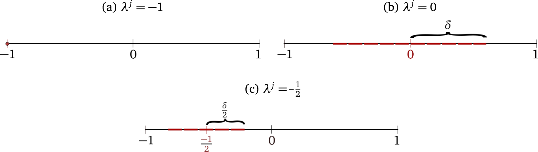

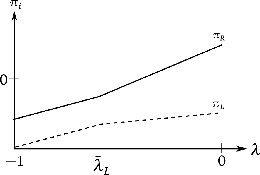


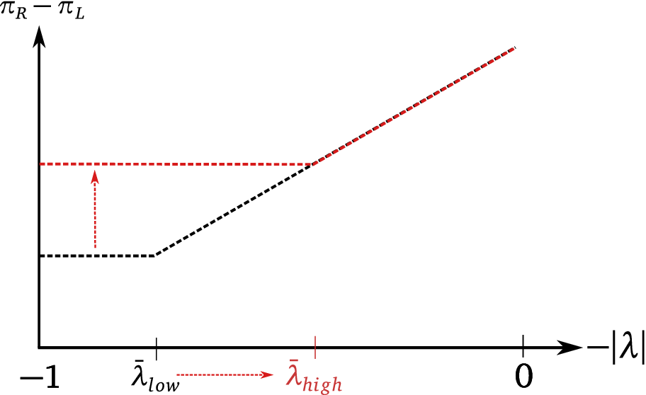


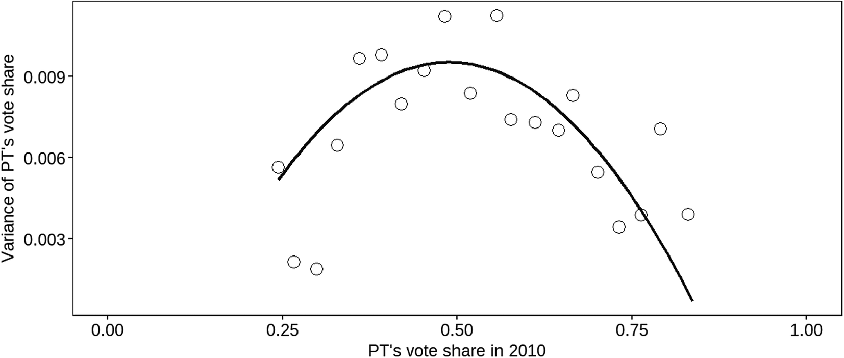
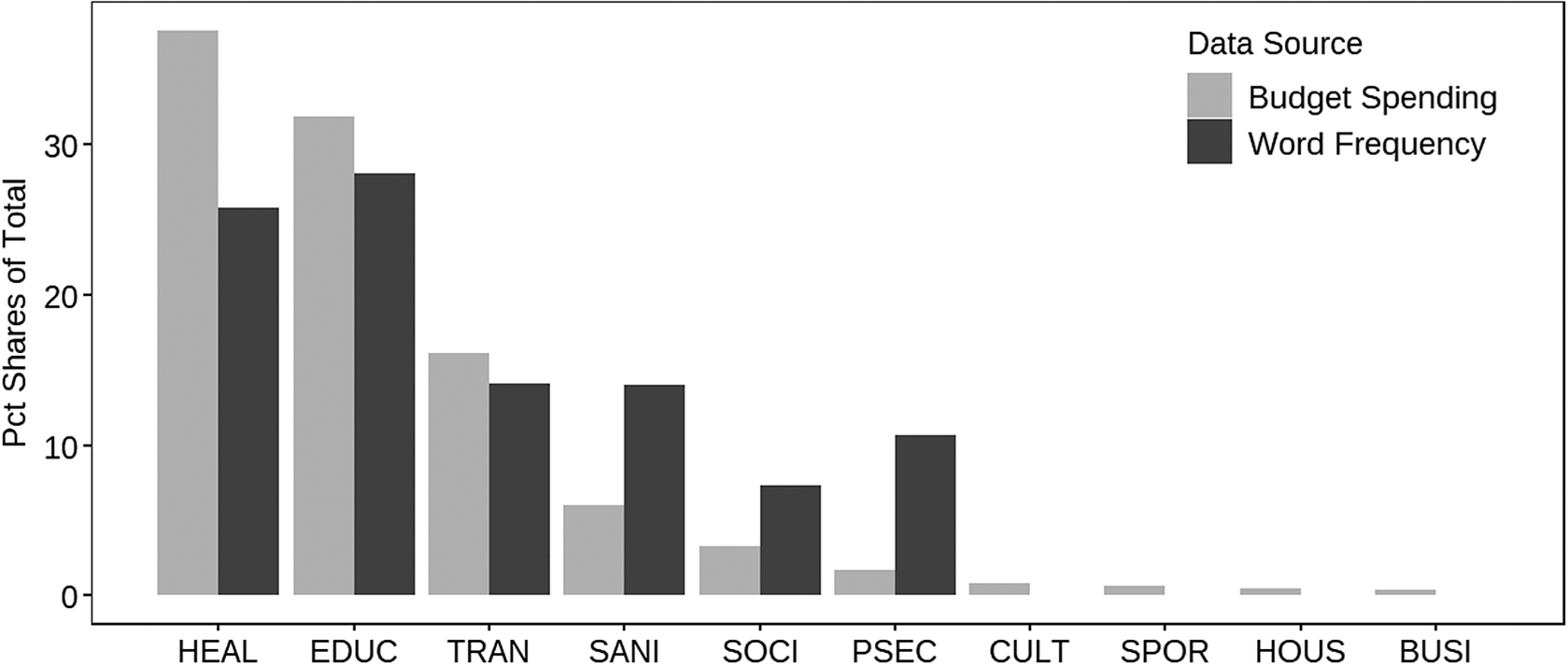
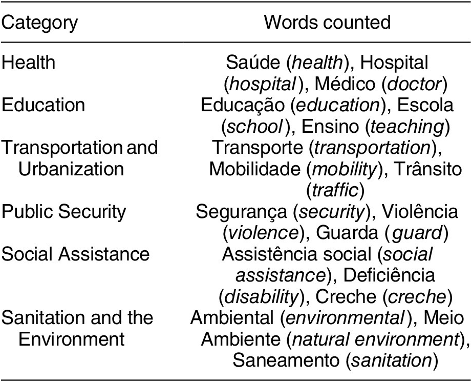

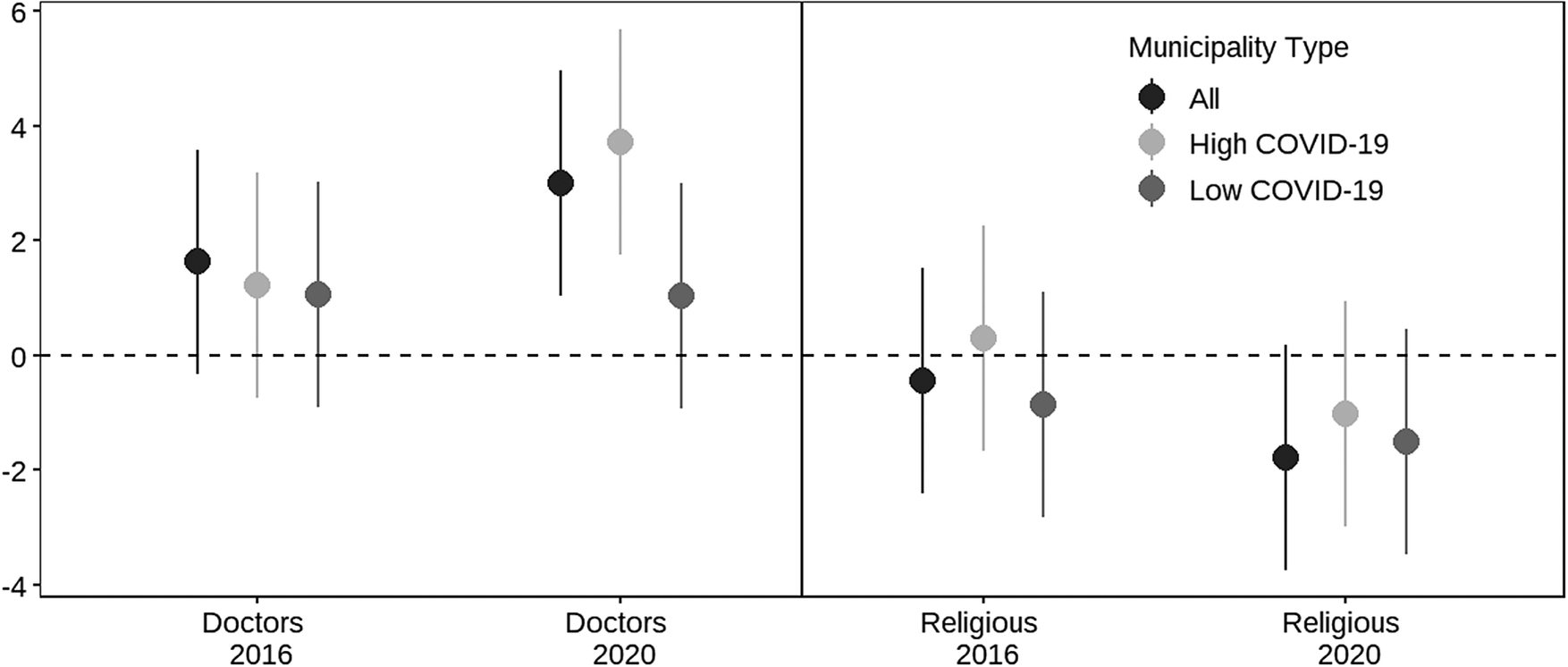


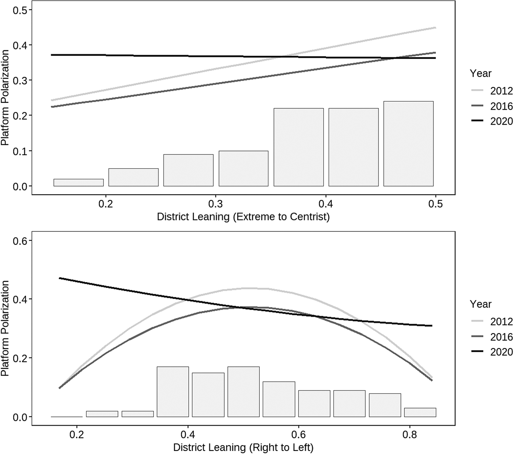
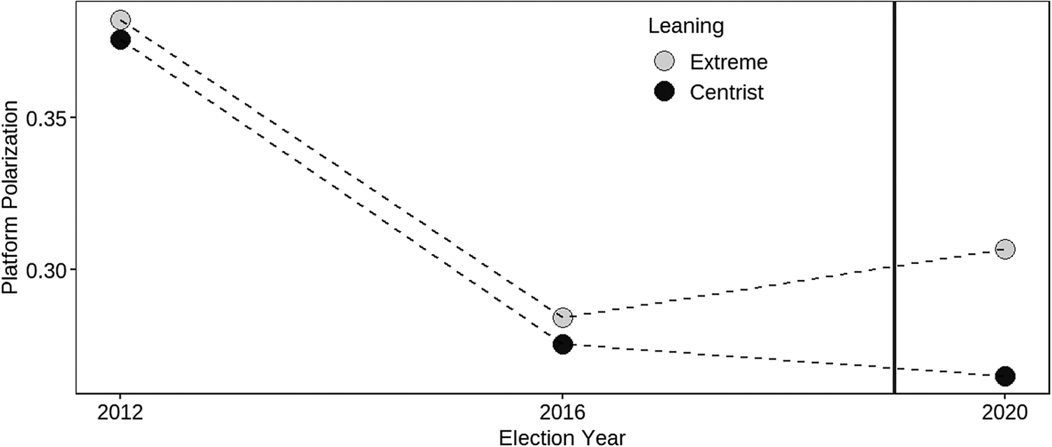
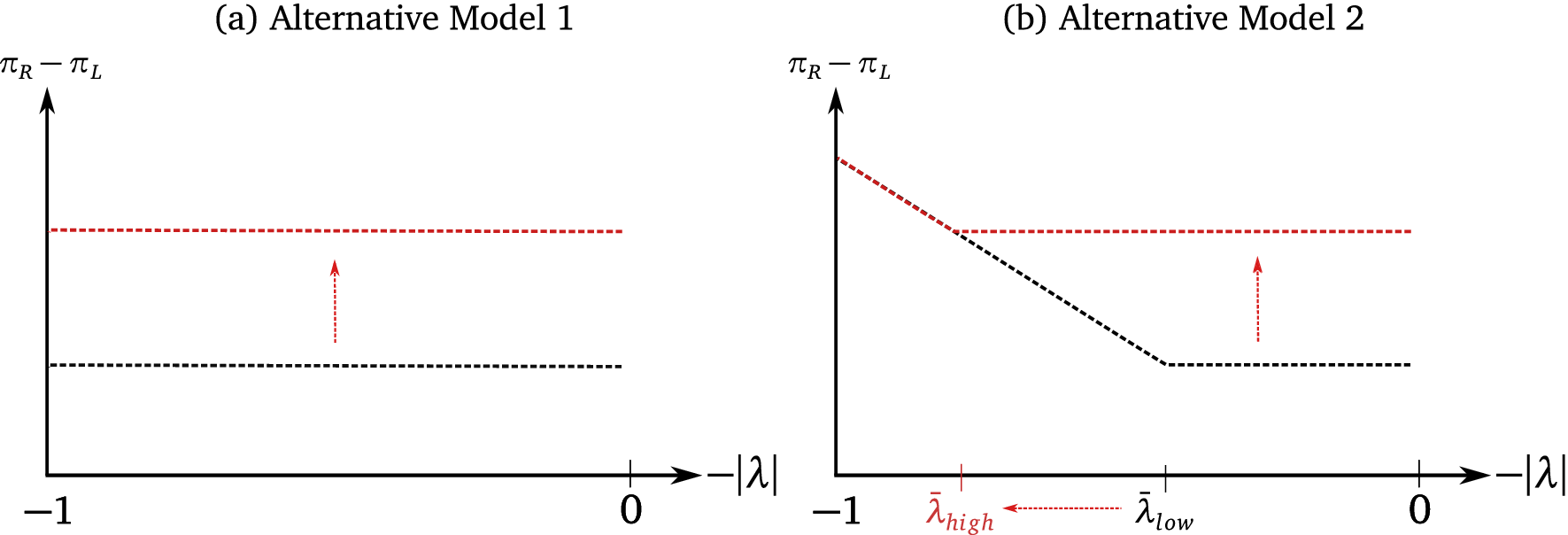


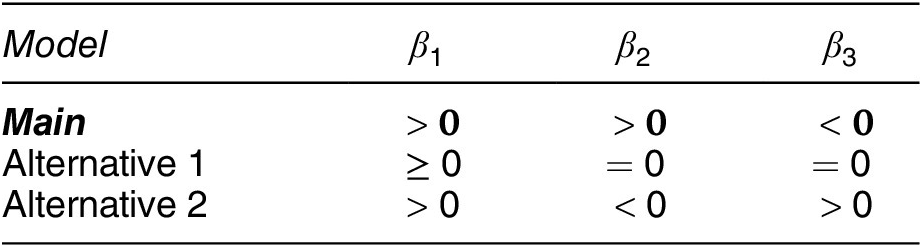
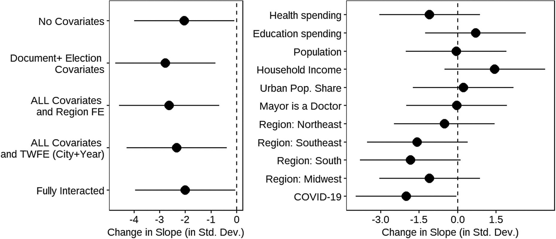


Comments
No Comments have been published for this article.