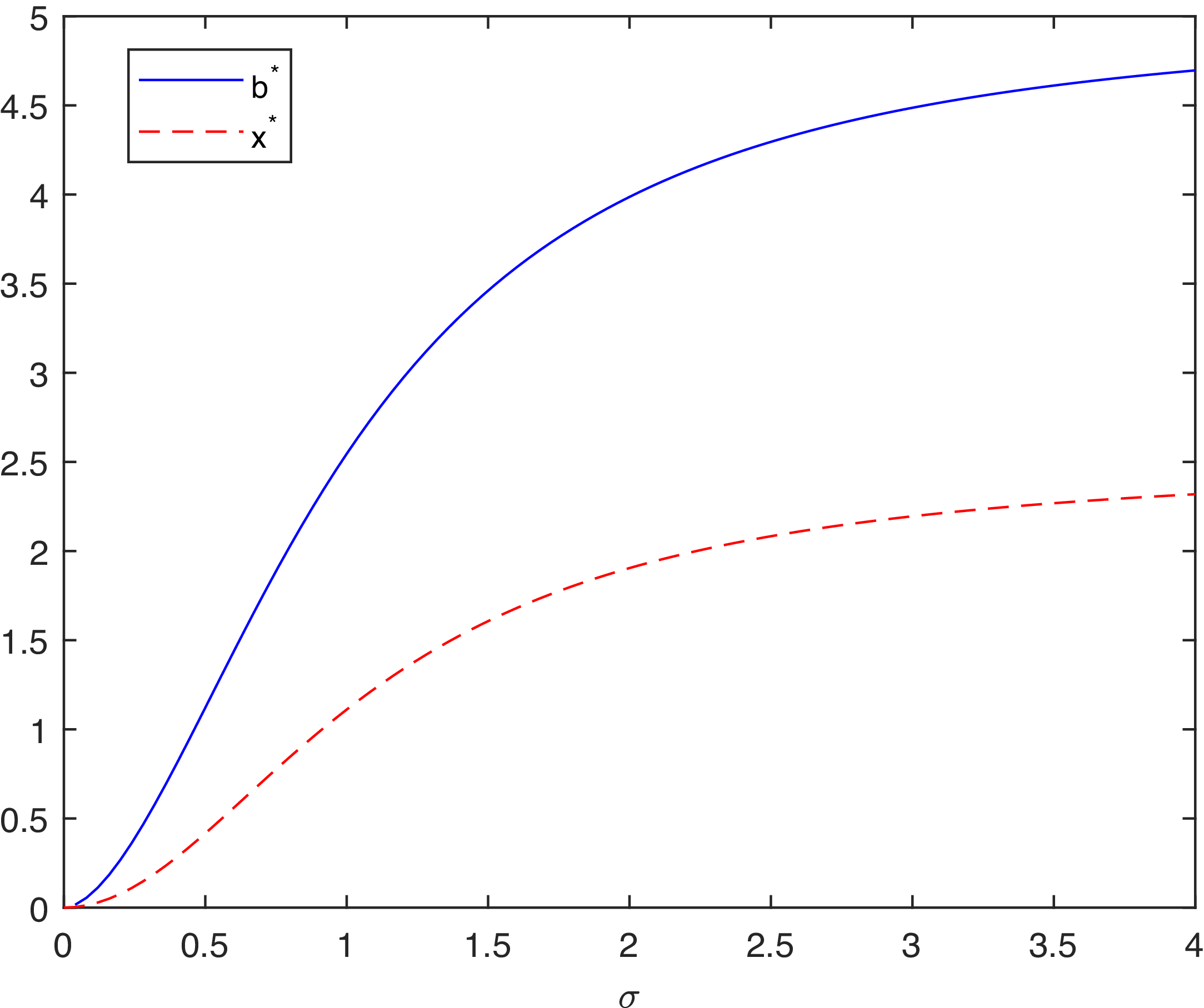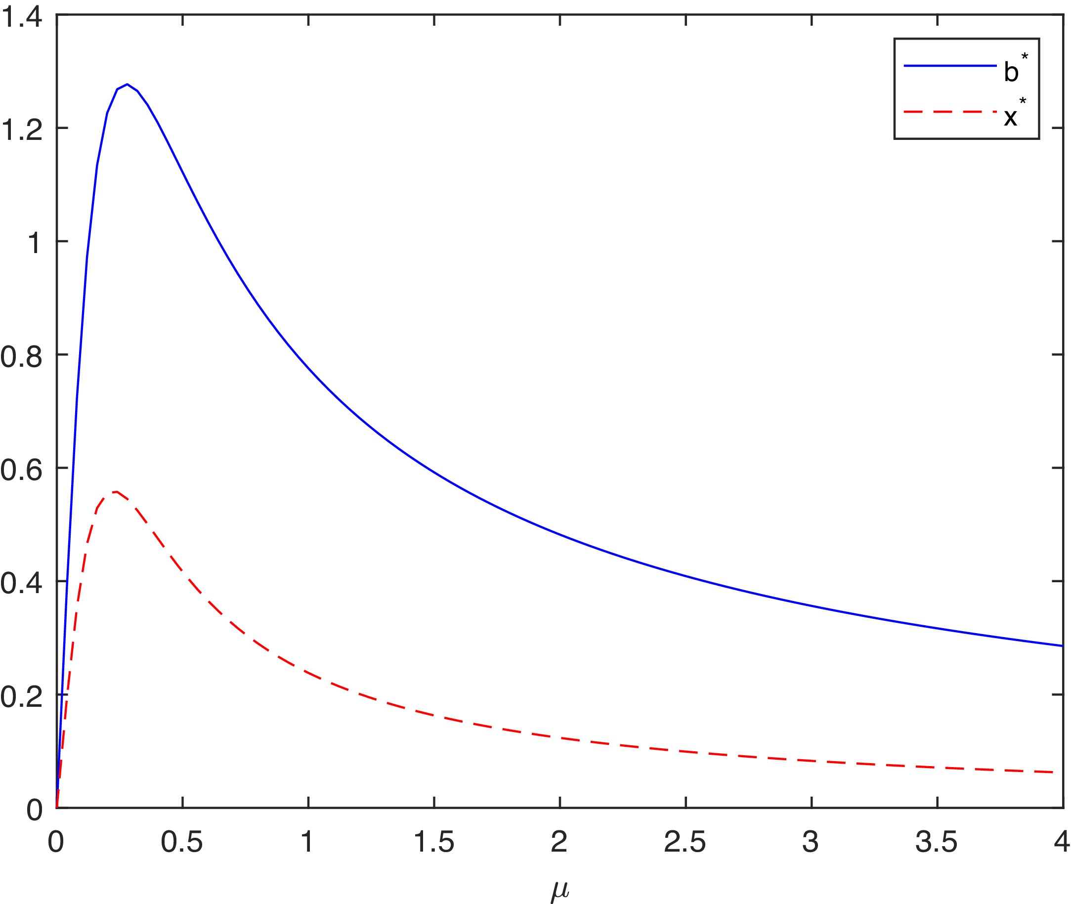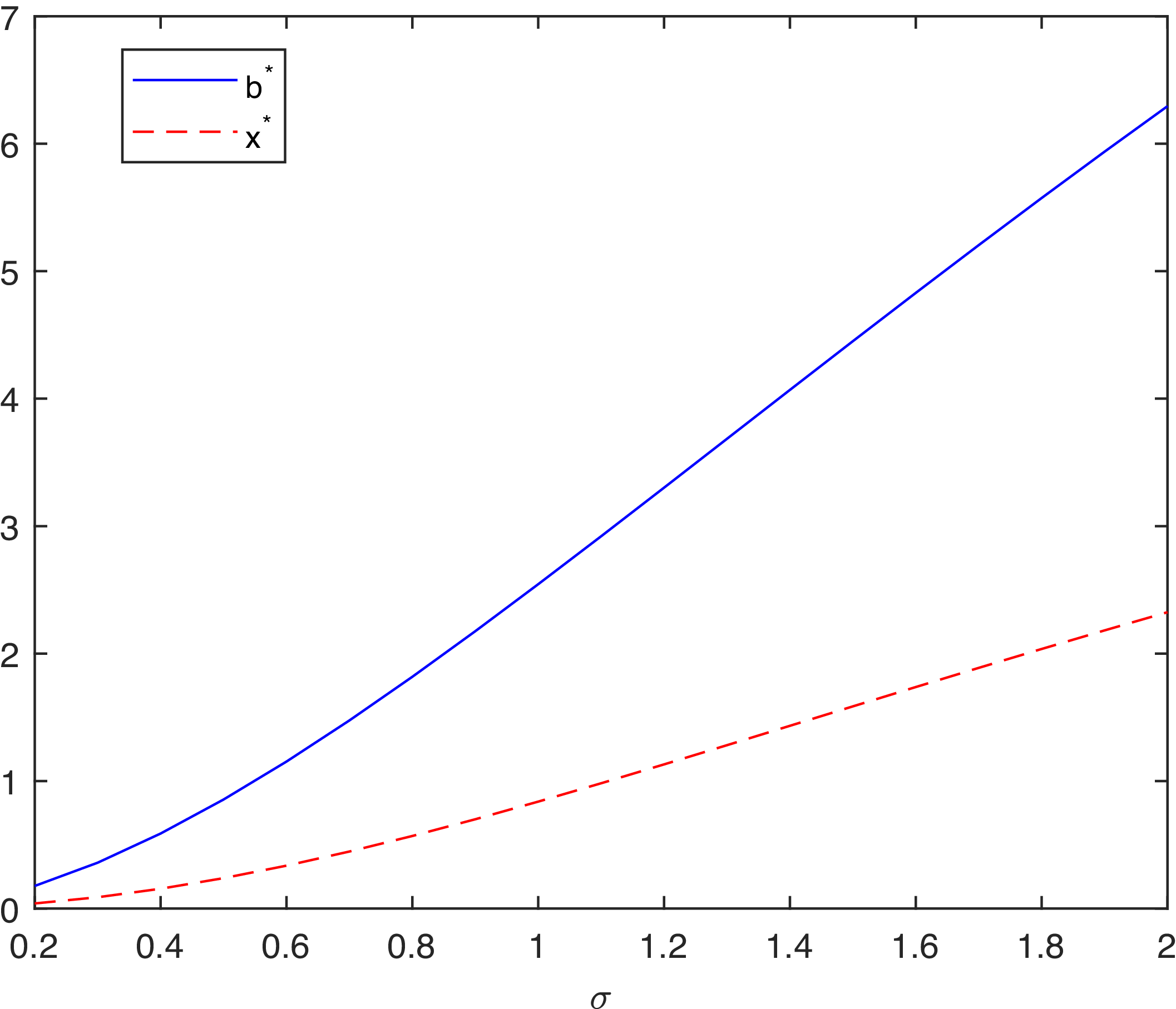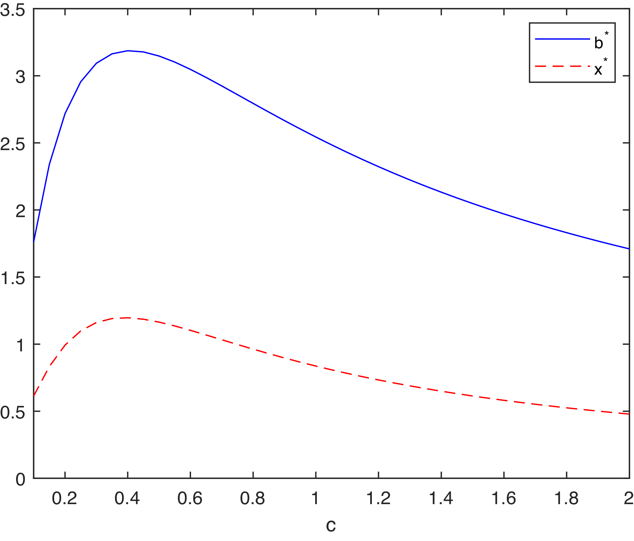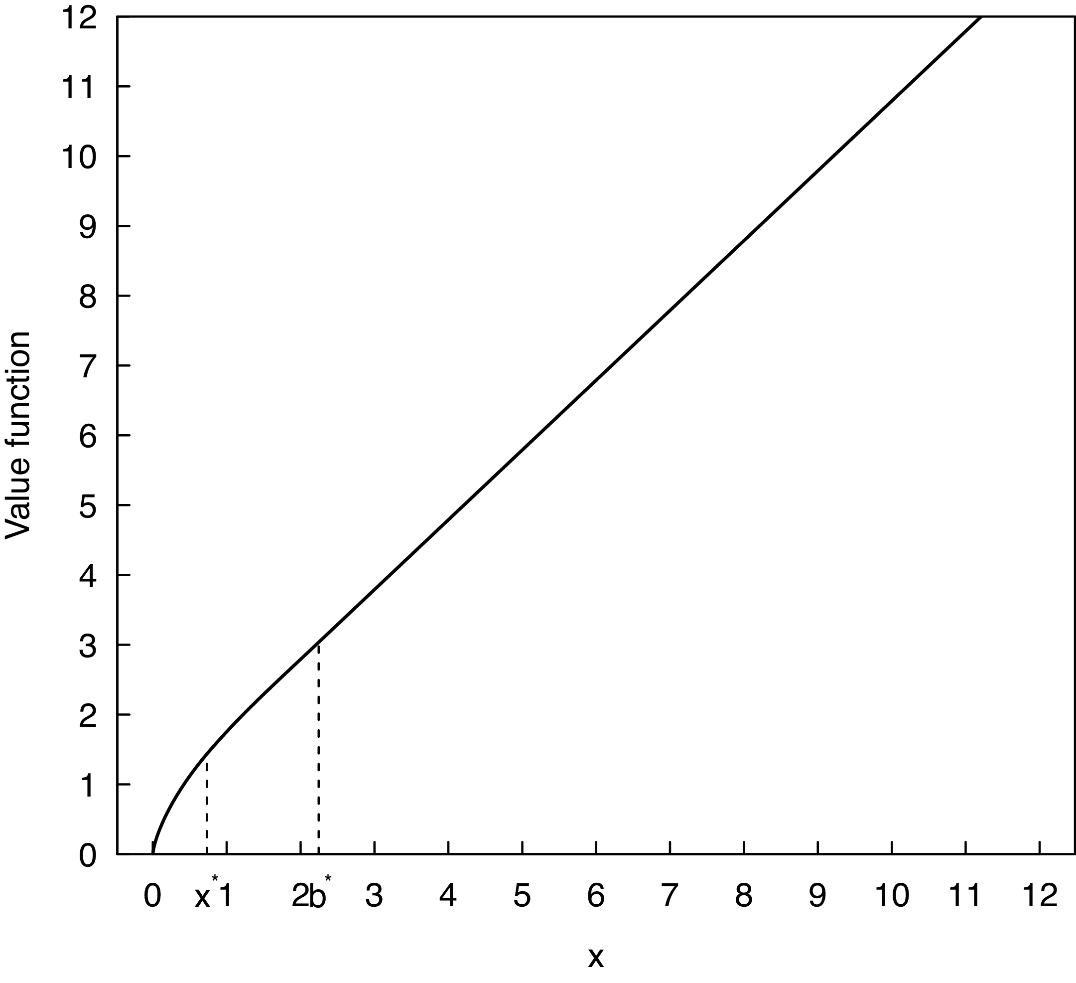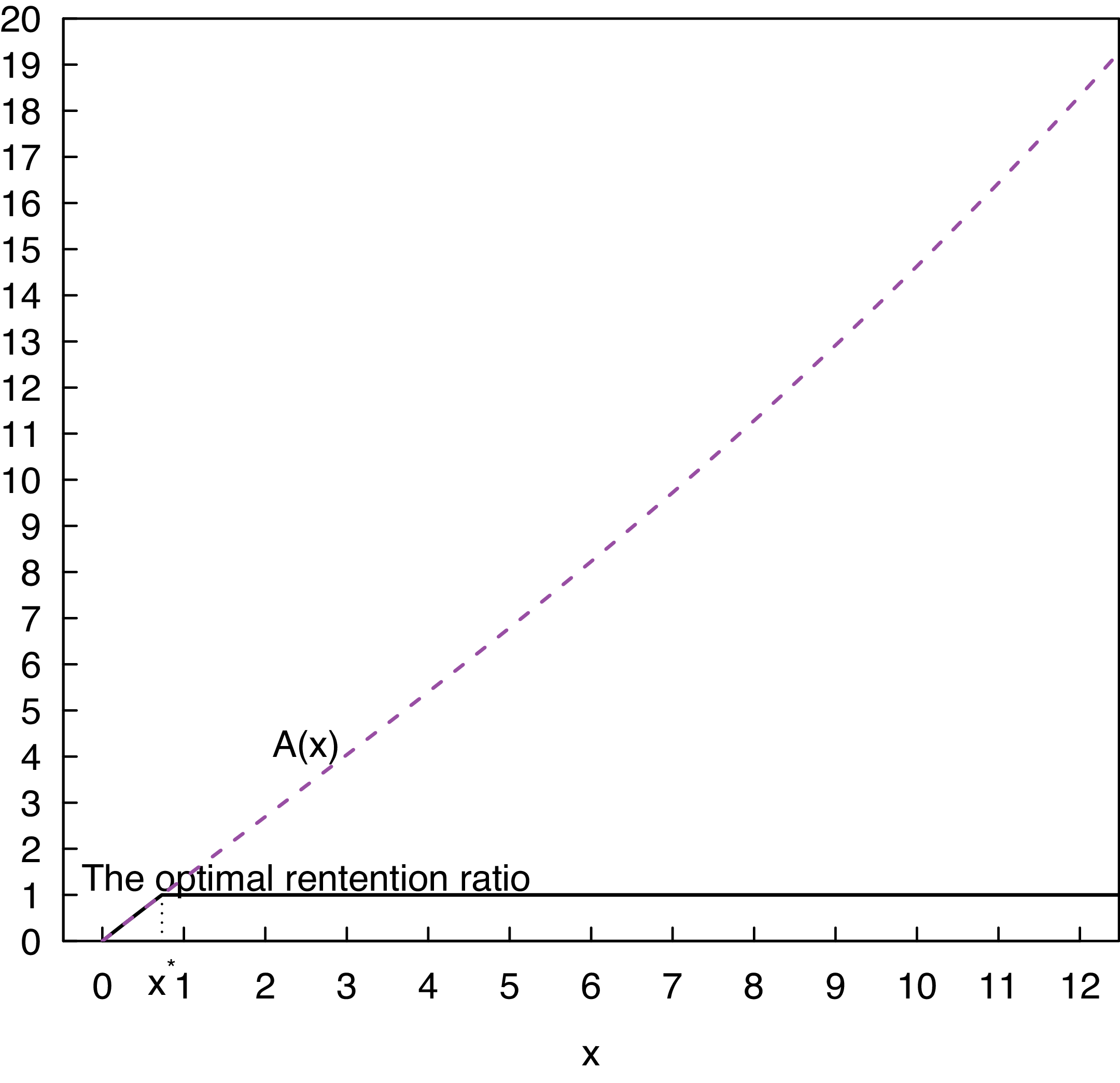



1. Introduction
We study a class of storage-type stochastic control problems with absorption risk, focusing on value maximization. The underlying state process follows a general diffusion, which is controlled in two ways: (i) by adjusting its operational scale through a scaling process that takes values in [0, 1]; and (ii) by subtracting a non-decreasing withdrawal process. The controlled process is absorbed once it reaches zero (or below). The objective is to maximize the discounted value of all withdrawals until the absorption time, or indefinitely if absorption never occurs.
This type of stochastic control problem has numerous applications across various fields, including optimal cash flow management in finance (cf. [Reference Asmussen, Højgaard and Taksar3, Reference Bai, Guo and Zhang4, Reference Cadenillas, Choulli, Taksar and Zhang6, Reference Chen, Yuen and Wang7, Reference Choulli, Taksar and Zhou10, Reference Liang and Young17, Reference Radner and Shepp22, Reference Taksar and Zhou26]), harvesting planning (cf. [Reference Alvarez2]), and reservoir management, with the latter two generally involving only the control in (ii). In these contexts, the underlying process typically represents capital or reserves in a company, fluctuating populations in harvesting problems or water levels in a reservoir. In particular, these problems are closely related to the study of optimal dynamic risk exposure control and cash flow management, where the objective is to maximize the expected firm value. Firms strategically manage their risk exposure through business activities and/or risk-sharing mechanisms to optimize various objective functions (see, for example, [Reference Choulli, Taksar and Zhou10, Reference Radner and Shepp22, Reference Wang, Chen, Chiu and Wong27, Reference Bai, Zhou, Xiao, Gao and Zhong28]). This application has attracted significant attention over the past few decades, with some of the earliest contributions dating back to [Reference Radner and Shepp22, Reference Taksar and Zhou26]. In the standard setting, a firm’s liquid reserves are modeled as a diffusion process, where the drift term represents expected profit and the diffusion coefficient reflects risk exposure. The firm controls its risk exposure by adjusting the diffusion coefficient, which simultaneously affects expected profit in the same direction. Extensive literature exists on risk exposure control, including the use of reinsurance as a risk management tool to maximize firm value (see, for example, [Reference Asmussen, Højgaard and Taksar3, Reference Bai, Guo and Zhang4, Reference Cadenillas, Choulli, Taksar and Zhang6, Reference Chen, Yuen and Wang7, Reference Choulli, Taksar and Zhou9, Reference Choulli, Taksar and Zhou10, Reference Feng, Zhu and Siu12, Reference Guo13, Reference Liang and Young17, Reference Radner and Shepp22, Reference Taksar and Zhou26, Reference Yao, Yang and Wang29, Reference Zhou and Yuen31]).
Despite the extensive attention devoted to this type of optimal control problem in the literature, much of the research concerning the controls in both (i) and (ii) above has concentrated on models driven by Brownian motion. Surprisingly, there is still a lack of theoretical studies that address the value-maximization storage-type optimal control of risk exposure/operational scale, and withdrawals in more general and realistic diffusion models that extend beyond the Brownian framework. This paper aims to fill this gap by investigating this class of optimal control problem under a general linear diffusion model, with the goal of deriving explicit theoretical optimality results within this broader setting.
While Brownian motion plays a foundational role in stochastic modeling due to its analytical tractability, it is often too restrictive to accurately capture many real-world phenomena. For example, Brownian motion-based surplus models typically neglect investment or interest income on cash reserves and fail to capture the dependence of returns and volatility on the level of available capital. Although some progress has been made, relatively few studies have explored optimal operational scale and withdrawal strategies within models that move beyond the Brownian motion assumption.
In this paper, we take a step toward addressing this gap by studying a class of optimal operational scale and withdrawal control problems within a general diffusion framework. This class of models includes the classical Brownian motion model as a special case while allowing for more general dynamics, such as state-dependent drift and volatility. We show that these problems can be solved theoretically within this more flexible framework, thereby extending the scope of optimal control results to a wider array of diffusion-based models commonly used in finance and insurance. Our analysis is built upon a general diffusion framework, where both the drift and volatility coefficients are allowed to vary as general functions of the state (or storage) process. This level of generality accommodates a variety of models and enables a unified treatment of optimal control problems across different settings. We demonstrate that, even in this broader context, the optimal control problem is solvable and that the optimal solution to the optimization problem can be obtained through a theoretical approach.
We begin by conjecturing that the positive real line can be divided into three regions: the partial-scale region, the full-scale region, and the withdrawal region. We then theoretically establish the existence of, or implicitly construct, candidate solutions to the Hamilton–Jacobi–Bellman (HJB) equation in each region for any given thresholds. Without requiring explicit closed-form solutions, we derive key theoretical properties of these solutions. A global candidate solution is constructed by smoothly pasting the local solutions across the three regions. By appropriately setting the thresholds, we prove that this global solution satisfies the necessary conditions to be the optimal solution. Our theoretical results hold in a general setting and apply to a broad class of problems. To illustrate the applicability of our approach, we provide examples where explicit solutions can be derived, as well as cases where explicit forms are unavailable within our proposed framework.
This work makes several contributions. We solve a class of value-maximizing optimal control problems involving operational scale/risk exposure, and withdrawals under a generalized diffusion framework. This framework accommodates a broad range of scenarios, including traditional Brownian motion as well as more general diffusion processes. Our approach yields either explicit or semi-explicit solutions. We develop a comprehensive and unified mathematical methodology for addressing these optimization problems. A rigorous and implementable procedure is provided for identifying solutions, whether in cases where closed-form solutions exist or where fully explicit expressions are not obtainable. In addition, we derive necessary and sufficient conditions for the existence of explicit solutions. Finally, to demonstrate the applicability of our results, we present a variety of examples, some rooted in classical settings, and others representing novel scenarios that reflect diverse business contexts for which, to the best of our knowledge, no prior solutions exist.
The remainder of the paper is organized as follows. In Section 2, we introduce the dynamic model and formulate the storage-type value-maximizing operational scale and withdrawals control problem. We divide the analysis into three scenarios based on the behavior of the drift rate: (i) when the drift rate is strictly positive for all levels of storage, (ii) when the drift rate is non-positive at zero storage, and (iii) when the drift becomes negative at some point despite being positive at the origin (zero storage level). These cases are examined in detail in Sections 3–5, where we present the mathematical derivations, optimality results, and semi-explicit forms of the solutions in the general setting. In Section 6, we identify the necessary and sufficient conditions for the availability of fully explicit solutions. Section 7 summarizes the general procedure for solving the optimal control problem. In Section 8, we illustrate the results through several examples, including cases where explicit solutions are available. We also apply the general framework and solution procedure to well-known models of practical interest, such as the Brownian motion model and the Ornstein–Uhlenbeck process. For models where explicit solutions are not tractable, we demonstrate how the same methodology can be used to derive numerical approximations, supported by examples across various scenarios. Section 10 concludes the paper. All technical proofs are provided in the Appendix.
2. Problem formulation
Let $(\Omega, \mathcal{F}, {\mathrm{P}})$
denote a probability space, where all the random variables involved are defined. Let
$(\Omega, \mathcal{F}, {\mathrm{P}})$
denote a probability space, where all the random variables involved are defined. Let ${\mathrm{E}}$
represent the expectation associated with
${\mathrm{E}}$
represent the expectation associated with ${\mathrm{P}}$
. Define
${\mathrm{P}}$
. Define $W=\{W_t\}_{t\ge 0}$
to be a standard Brownian motion and let
$W=\{W_t\}_{t\ge 0}$
to be a standard Brownian motion and let $\mathcal{F}^W$
denote the augmented complete filtration generated by W. Consider the controlled stochastic process
$\mathcal{F}^W$
denote the augmented complete filtration generated by W. Consider the controlled stochastic process $ X_t^{\pi,L}$
governed by the stochastic differential equation (SDE):
$ X_t^{\pi,L}$
governed by the stochastic differential equation (SDE):
 \begin{eqnarray} {\mathrm{d}} X_t^{\pi,L}=\pi_{t} \big(\mu\big(X_{t-}^{\pi,L}\big){\mathrm{d}} t+ \sigma\big(X_{t-}^{\pi,L}\big){\mathrm{d}} W_t\big)- {\mathrm{d}} L_t,\quad t\ge 0,\end{eqnarray}
where $\pi_t$
is
$\pi_t$
is $\mathcal{F}^W_t$
-predictable with
$\mathcal{F}^W_t$
-predictable with $\pi_t\in[0,1]$
,
$\pi_t\in[0,1]$
, $L_t$
is an
$L_t$
is an $\mathcal{F}^W$
-predictable, non-decreasing, and cádlág (right-continuous with left limits) stochastic process with
$\mathcal{F}^W$
-predictable, non-decreasing, and cádlág (right-continuous with left limits) stochastic process with $L_{0-}=0$
.
$L_{0-}=0$
.
We define the hitting time:
 \begin{align}\tau^{\pi,L}=\inf \big\{t\ge 0\,:\, X^{\pi,L}_t<0 \big\}.\end{align}
This hitting time has a natural interpretation in both harvesting planning and reservoir management problems, as it represents the time of extinction and exhaustion, respectively, naturally marking the end of the process. In financial applications, when $ X_t $
represents cash reserves, this is the time when reserves hit zero. At this point, we assume the business ceases operations, due to forced liquidation resulting from reserve constraints, as assumed in [Reference Pierre, Villeneuve and Warin20].
$ X_t $
represents cash reserves, this is the time when reserves hit zero. At this point, we assume the business ceases operations, due to forced liquidation resulting from reserve constraints, as assumed in [Reference Pierre, Villeneuve and Warin20].
We assume the following standard conditions on $\mu(\!\cdot\!)$
and
$\mu(\!\cdot\!)$
and $\sigma(\!\cdot\!)$
: both
$\sigma(\!\cdot\!)$
: both $\mu(x)$
and
$\mu(x)$
and $\sigma(x)$
are Lipschitz continuous on
$\sigma(x)$
are Lipschitz continuous on $[0,\infty)$
and grow no faster than linearly in x, and
$[0,\infty)$
and grow no faster than linearly in x, and $\sigma(\!\cdot\!)$
is positive and non-vanishing on
$\sigma(\!\cdot\!)$
is positive and non-vanishing on $[0,\infty)$
. These conditions guarantee that, for an initial state
$[0,\infty)$
. These conditions guarantee that, for an initial state $X_{0-}=x$
, and a pair
$X_{0-}=x$
, and a pair $(\pi,L)$
(with
$(\pi,L)$
(with $\pi_t$
being
$\pi_t$
being $\mathcal{F}^W$
-predictable and
$\mathcal{F}^W$
-predictable and $L_t$
being
$L_t$
being $\mathcal{F}^W$
-predictable, non-decreasing, and cádlág) there exists a unique strong solution to the SDE (1) on
$\mathcal{F}^W$
-predictable, non-decreasing, and cádlág) there exists a unique strong solution to the SDE (1) on $0\le t\le \tau^{\pi,L}$
(see pp. 37–39 of [Reference Pham21]).
$0\le t\le \tau^{\pi,L}$
(see pp. 37–39 of [Reference Pham21]).
In the above setup, the pair $(\pi,L)\,:\!=\,(\{\pi_t\}_{t\ge 0},\{L_t\}_{t\ge 0})$
is referred to as the control law, and
$(\pi,L)\,:\!=\,(\{\pi_t\}_{t\ge 0},\{L_t\}_{t\ge 0})$
is referred to as the control law, and $X^{\pi,L}\,:\!=\,\{X_t^{\pi,L}\}_{t\ge 0}$
is called the controlled state process.
$X^{\pi,L}\,:\!=\,\{X_t^{\pi,L}\}_{t\ge 0}$
is called the controlled state process.
The formulation above describes a controlled stochastic process commonly used in financial modeling, inventory control, and reservoir management. The state variable $X^{\pi,L}_t$
can represent the capital or reserves in a company, inventory levels, or water in a reservoir. The control variable
$X^{\pi,L}_t$
can represent the capital or reserves in a company, inventory levels, or water in a reservoir. The control variable $\pi_t$
might represent risk exposure or business scale in problems such as consumption, cash withdrawal, or dividends distribution; the proportion of resources allocated to inventory replenishment; or the proportion of inflow directed to storage, among other interpretations. The variable
$\pi_t$
might represent risk exposure or business scale in problems such as consumption, cash withdrawal, or dividends distribution; the proportion of resources allocated to inventory replenishment; or the proportion of inflow directed to storage, among other interpretations. The variable $L_t$
represents the cumulative amount of consumption, cash withdrawal, or dividend payments; non-decreasing adjustments due to external supply, corrections to maintain nonnegativity, or a release process.
$L_t$
represents the cumulative amount of consumption, cash withdrawal, or dividend payments; non-decreasing adjustments due to external supply, corrections to maintain nonnegativity, or a release process.
We formally define admissible control laws as follows.
Definition 1. (Admissible strategies.) Define $\mathcal{A}$
to be the set of all admissible strategies,
$\mathcal{A}$
to be the set of all admissible strategies, $(\pi,L)$
, that satisfy the following conditions: (a)
$(\pi,L)$
, that satisfy the following conditions: (a) $(\pi,L)$
is
$(\pi,L)$
is $\mathcal{F}^W$
-predictable; (b)
$\mathcal{F}^W$
-predictable; (b) $\pi_t\in[0,1]$
; (c) L is everywhere right-continuous and has left limits everywhere (cádlág); and (d)
$\pi_t\in[0,1]$
; (c) L is everywhere right-continuous and has left limits everywhere (cádlág); and (d) $L_{0-}=0$
, L is non-decreasing and
$L_{0-}=0$
, L is non-decreasing and $L_t-L_{t-}\le X^{\pi,L}_{t-}$
.
$L_t-L_{t-}\le X^{\pi,L}_{t-}$
.
Item (a) indicates that decisions at any time t depend solely on historical information before time t and item (b) states that the decision-maker can adjust the business scale or exposure ratio anywhere between 0% and 100%. Item (c) implies that if there is a lump sum withdrawal at time t, this amount is treated as a deduction at time $t-$
, which reduces the state level immediately before time t. Finally, item (d) specifies that all withdrawals must be non-negative, and the amount of each withdrawal cannot exceed the available quantity at the time of withdrawal. In other words, withdrawals cannot directly result in a deficit.
$t-$
, which reduces the state level immediately before time t. Finally, item (d) specifies that all withdrawals must be non-negative, and the amount of each withdrawal cannot exceed the available quantity at the time of withdrawal. In other words, withdrawals cannot directly result in a deficit.
We quantify the performance of the control law, $(\pi,L)$
, by the expected total discounted value
$(\pi,L)$
, by the expected total discounted value
 \begin{align}\mathcal{P}(\pi,L)(x)={\mathrm{E}}_x\bigg[\int_0^{\tau^{\pi,L}}\mathrm{e}^{-\delta t}\,{\mathrm{d}} L_t\bigg],\end{align}
where ${\mathrm{E}}_x$
represents the conditional expectation given
${\mathrm{E}}_x$
represents the conditional expectation given $X_{0-}=x$
:
$X_{0-}=x$
:
 \begin{align}{\mathrm{E}}_x[\!\cdot\!]={\mathrm{E}}[\!\cdot\!|X_{0-}=x],\end{align}
and $\delta>0$
is the discount rate used by the decision maker, reflecting their intertemporal preferences.
$\delta>0$
is the discount rate used by the decision maker, reflecting their intertemporal preferences.
The optimal control problem. The objective of the control problem is to maximize the performance functional
 \begin{align}\mathcal{P}(\pi,L)(x) ={\mathrm{E}}_x\bigg[\int_0^{\tau^{\pi,L}}\mathrm{e}^{-\delta t}\,{\mathrm{d}} L_t\bigg],\end{align}
over all admissible strategies $(\pi,L)\in\mathcal{A}$
, that is,
$(\pi,L)\in\mathcal{A}$
, that is,
 \begin{align}V(x)\,:\!=\,\sup\nolimits_{(\pi,L)\in\mathcal{A}}{\mathrm{E}}_x\bigg[\int_0^{\tau^{\pi,L}}\mathrm{e}^{-\delta t}\,{\mathrm{d}} L_t\bigg],\end{align}
subject to the system dynamics in (1) and the constraints imposed on admissible strategies as outlined in Definition 1. We refer to V as the value function. The value function, depending on the application context, can represent the maximum discounted profit, the maximum benefit, or the maximum utility of water release (e.g. for electricity generation or irrigation).
If there exists a control law, say $(\pi^*, L^*)$
, from the set of admissible strategies that attains the maximal performance, i.e.
$(\pi^*, L^*)$
, from the set of admissible strategies that attains the maximal performance, i.e.
 \begin{align}\mathcal{P}(\pi^*,L^*)(x)=\sup\nolimits_{(\pi,L)\in\mathcal{A}}{\mathrm{E}}_x\bigg[\int_0^{\tau^{\pi,L}}\mathrm{e}^{-\delta t} \, {\mathrm{d}} L_t\bigg],\end{align}
then $(\pi^*, L^*)$
is the optimal control law.
$(\pi^*, L^*)$
is the optimal control law.
The model underlying the control problem discussed above is quite general. It includes the widely studied Brownian motion model, where $\mu(\!\cdot\!)=\mathrm{constant}$
and
$\mu(\!\cdot\!)=\mathrm{constant}$
and $\sigma(\!\cdot\!)=\mathrm{ constant}$
, as well as the less commonly explored extension, the Ornstein–Uhlenbeck process. The latter corresponds to
$\sigma(\!\cdot\!)=\mathrm{ constant}$
, as well as the less commonly explored extension, the Ornstein–Uhlenbeck process. The latter corresponds to $\mu(x)=c_1 x+c_2$
for two constants
$\mu(x)=c_1 x+c_2$
for two constants $c_1$
and
$c_1$
and $c_2$
, which can represent more realistic dynamics in certain areas, e.g. finance and insurance, where cash reserves generate interest.
$c_2$
, which can represent more realistic dynamics in certain areas, e.g. finance and insurance, where cash reserves generate interest.
Following standard arguments in optimal control (see, for instance, [Reference Yong and Zhou30]), we derive the following HJB equation:
 \begin{align}\max\left\{ \max_{a\in[0,1]}\left(\frac{1}{2}\sigma^{2}(x) a^{2}\,f^{\prime\prime}(x)+\mu(x) a\,f^\prime(x)-\delta\,f(x)\right)\!, 1-f^\prime(x)\right\}\le 0.\end{align}
Intuitively, if the value function is sufficiently smooth, it should satisfy the above HJB equation with a corresponding to the risk exposure control $\pi$
. Note that given
$\pi$
. Note that given $X_{0-}=0$
, ruin occurs immediately, i.e.
$X_{0-}=0$
, ruin occurs immediately, i.e. $ \tau^{\pi,L}=0$
conditional on
$ \tau^{\pi,L}=0$
conditional on $X_{0-}=0$
. As a result, we have
$X_{0-}=0$
. As a result, we have
 \begin{align}V(0)=\sup\nolimits_{(\pi,L)\in\mathcal{A}}{\mathrm{E}}_0\bigg[\int_0^{\tau^{\pi,L}}\mathrm{e}^{-\delta t}\,{\mathrm{d}} L_t\bigg]=0.\end{align}
We conjecture that if V is sufficiently smooth, a heuristic conclusion would be that it solves the HJB equation. This motivates us to study the solution (if any) to the following initial value problem first. Applying a standard method in optimal control by using Itô lemma we can obtain the following verification theorem.
Theorem 1. (Verification theorem.) If f is a twice continuously differentiable function that satisfies:

then $f(x)\ge V(x)$
for
$f(x)\ge V(x)$
for $x\ge 0$
.
$x\ge 0$
.
In light of the above verification theorem, it is natural to first inquire whether such a function as described in the theorem exists. We attempt to answer this by searching for candidate solutions to the initial value HJB equation:
 \begin{align} &\max\left\{ \max_{a\in[0,1]}\left(\frac{1}{2}\sigma^{2}(x) a^{2}\,f^{\prime\prime}(x)+\mu(x) a\,f^\prime(x)-\delta\,f(x)\right)\!, 1-f^\prime(x)\right\}=0, \quad& x> 0, \end{align}
 \begin{align} &f(0)=0.\end{align}
A special case where both $\mu(x)$
and
$\mu(x)$
and $\sigma(x)$
are constants has been solved in [Reference Højgaard and Taksar14], who studied an optimal reinsurance and dividend problem for a Brownian motion with a constant positive drift and a constant diffusion coefficient. This leads to the same mathematical problem as the special case discussed here. Further variations of the problem under the Brownian motion framework (with constant drifts and volatilities, in absence of control) have been considered in [Reference Asmussen, Højgaard and Taksar3, Reference Bai, Guo and Zhang4, Reference Cadenillas, Choulli, Taksar and Zhang6, Reference Choulli, Taksar and Zhou9–Reference Choulli, Taksar and Zhou11, Reference Højgaard and Taksar15, Reference Liang and Young17, Reference Meng and Siu18, Reference Taksar25, Reference Taksar and Zhou26], among others.
$\sigma(x)$
are constants has been solved in [Reference Højgaard and Taksar14], who studied an optimal reinsurance and dividend problem for a Brownian motion with a constant positive drift and a constant diffusion coefficient. This leads to the same mathematical problem as the special case discussed here. Further variations of the problem under the Brownian motion framework (with constant drifts and volatilities, in absence of control) have been considered in [Reference Asmussen, Højgaard and Taksar3, Reference Bai, Guo and Zhang4, Reference Cadenillas, Choulli, Taksar and Zhang6, Reference Choulli, Taksar and Zhou9–Reference Choulli, Taksar and Zhou11, Reference Højgaard and Taksar15, Reference Liang and Young17, Reference Meng and Siu18, Reference Taksar25, Reference Taksar and Zhou26], among others.
We distinguish among three cases, (a) $\mu(x)>0$
for all
$\mu(x)>0$
for all $x\ge 0$
, (b)
$x\ge 0$
, (b) $\mu(0)\le 0$
, and (c)
$\mu(0)\le 0$
, and (c) $\mu(0)>0$
and
$\mu(0)>0$
and $\mu(x) \le 0$
for some
$\mu(x) \le 0$
for some $x>0$
, and analyze them separately. In our analysis, we also impose the following condition on the drift coefficient function.
$x>0$
, and analyze them separately. In our analysis, we also impose the following condition on the drift coefficient function.
Assumption 1. We assume $\mu^\prime(x) < \delta$
.
$\mu^\prime(x) < \delta$
.
This assumption is introduced for mathematical tractability and is also considered natural in financial modeling, as discussed in [Reference Paulsen19] and also due to the fact that in the context of profit testing, the subjective discount rate $\delta$
used to value future cash flows by the shareholders typically exceeds the growth rate (the force of growth) of a risk business,
$\delta$
used to value future cash flows by the shareholders typically exceeds the growth rate (the force of growth) of a risk business, $\mu'$
, by a risk margin.
$\mu'$
, by a risk margin.
3. Optimality results when $\boldsymbol\mu(\boldsymbol{x}) > 0$
for all
$\boldsymbol{x} \ge 0$
$\boldsymbol\mu(\boldsymbol{x}) > 0$
for all
$\boldsymbol{x} \ge 0$


We consider the case $\mu(x)>0$
for all
$\mu(x)>0$
for all $x\ge 0$
throughout the whole section. We start with constructing a strictly increasing and strictly concave solution to
$x\ge 0$
throughout the whole section. We start with constructing a strictly increasing and strictly concave solution to
 \begin{align}&\max_{a\in[0,1]}\left(\frac{1}{2}a^2\sigma^2(x)\,f^{\prime\prime}(x)+\mu(x) a\,f^\prime(x)-\delta\,f(x)\right)=0,\quad\mbox{for $x\in (0,x_{1}]$},\quad f(0)=0, \end{align}
where $x_1$
is a positive constant that is determined later. Suppose the desired solution exists, denoted by f(x) here. Noting that this function, f, is strictly concave, we have
$x_1$
is a positive constant that is determined later. Suppose the desired solution exists, denoted by f(x) here. Noting that this function, f, is strictly concave, we have $f^{\prime\prime}(x)<0$
for
$f^{\prime\prime}(x)<0$
for $x\in (0,x_1]$
and thus we can see
$x\in (0,x_1]$
and thus we can see
 \begin{align*}\arg\max_a\left(\frac{1}{2}a^{2}\sigma^{2}(x)\,f^{\prime\prime}(x)+\mu(x) a\,f^\prime(x)-\delta\,f(x))\right)=-\frac{\mu(x)}{\sigma^{2}(x)} \frac{ f^\prime(x)}{f^{\prime\prime}(x)},\quad x\in(0,x_1].\end{align*}
Define
 \begin{align}a_{f}(x)=-\frac{\mu(x)}{\sigma^{2}(x)} \frac{ f^\prime(x)}{f^{\prime\prime}(x)}.\end{align}
Suppose there exists an $x_{1}>0$
such that
$x_{1}>0$
such that $a_f(x)\in[0,1]$
for
$a_f(x)\in[0,1]$
for $x\in[0,x_1]$
(the existence of such
$x\in[0,x_1]$
(the existence of such $x_1$
will be verified later after we obtain a candidate expression for the desired f(x)). Then,
$x_1$
will be verified later after we obtain a candidate expression for the desired f(x)). Then,
 \begin{align}\arg\max_{a\in[0,1]}\left(\frac{1}{2}a^{2}\sigma^{2}(x)\,f^{\prime\prime}(x)+\mu(x) a\,f^\prime(x)-\delta\,f(x)\right)=a_{f}(x), \quad x\in (0,x_{1}].\end{align}
Thus, by combining (15) with the assumption that f is a solution to (13) we obtain
 \begin{align}\frac{1}{2}a_{f}^{2}(x)\sigma^{2}(x)\,f^{\prime\prime}(x)+\mu(x) a_{f}(x)\,f^\prime(x)-\delta\,f(x)=0,\quad x\in (0,x_{1}].\end{align}
From (14), we have
 \begin{align}\sigma^{2}(x)\,f^{\prime\prime}(x)=-\frac{\mu(x)\,f^\prime(x)}{a_{f}(x)}.\end{align}
Substituting (17) into (16) yields
 \begin{align}\frac{1}{2}a_{f}(x)\mu(x)\,f^\prime(x)-\delta\,f(x)=0, \quad x\in (0,x_{1}].\end{align}
Differentiating (18) with respect to x gives
 \begin{align}\frac{1}{2}a_{f}(x)\mu(x)\,f^{\prime\prime}(x)+\left(\frac{1}{2}\mu^\prime(x)a_{f}(x)+\frac12\mu(x)a_{f}^\prime(x)-\delta\right)\!f^\prime(x)=0, \quad x\in (0,x_{1}].\end{align}
From (17) we get
 $$a_{f}(x)\,f^{\prime\prime}(x)=-\frac{\mu(x)\,f^\prime(x)}{\sigma^{2}(x)}.$$
By substituting this into (19) we get
 \begin{align}\left(-\frac{1}{2}\frac{\mu^{2}(x)}{\sigma^{2}(x)}+\frac{1}{2}\mu^\prime(x)a_{f}(x)+\frac{1}{2}\mu(x)a_{f}^\prime(x)-\delta\right)\!f^\prime(x)=0, \quad x\in (0,x_{1}].\end{align}
Recall that f is strictly increasing on $[0,x_1]$
and so we know
$[0,x_1]$
and so we know $f^\prime(x)>0 $
for
$f^\prime(x)>0 $
for $x\in (0,x_1]$
. Thus, it follows from (20) that
$x\in (0,x_1]$
. Thus, it follows from (20) that
 $$-\frac{1}{2}\frac{\mu^{2}(x)}{\sigma^{2}(x)}+\frac{1}{2}\mu^\prime(x)a_{f}(x)+\frac{1}{2}\mu(x)a_{f}^\prime(x)-\delta=0, \quad x\in (0,x_{1}],$$
which implies
 $$\mu^\prime(x)a_{f}(x)+\mu(x)a_{f}^\prime(x)=2\delta+\frac{\mu^{2}(x)}{\sigma^{2}(x)},\quad \mbox{for $0< x\leq x_{1}$.}$$
That is,
 $$\frac{\mathrm{d}(\mu(x)a_f(x))}{\mathrm{d} x}=2\delta+\frac{\mu^{2}(x)}{\sigma^{2}(x)}\quad \mbox{for $0< x\le x_1$.}$$
Solving this differential equation gives
 \begin{align}a_{f}(x)=\frac{1}{\mu(x)}\bigg[\int_{0}^{x}\bigg(2\delta+\frac{\mu^{2}(y)}{\sigma^{2}(y)}\bigg)\mathrm{d} y+\mu(0)a_f(0)\bigg], \quad x\in[0, x_{1}].\end{align}
From (17) we know
 $$\frac{f^{\prime\prime}(x)}{f^\prime(x)}=-\frac{\mu(x)}{\sigma^{2}(x)a_{f}(x)}.$$
By solving this equation we have
 \begin{align}f(x)=C_{1}-C_{2}\int_{x}^{x_1}\exp\!\bigg({\int_{z}^{x_1}\frac{\mu(y)}{\sigma^{2}(y)a_{f}(y)}\,\mathrm{d} y}\bigg)\mathrm{d} z, \quad x\in(0, x_{1}].\end{align}
Since we want $f(0)=0$
and so
$f(0)=0$
and so
 $$C_{1}=C_{2}\int_{0}^{x_1}\exp\!\bigg({\int_{z}^{x_1}\frac{\mu(y)}{\sigma^{2}(y)a_{f}(y)}\,\mathrm{d} y}\bigg)\mathrm{d} z$$
and thus
 \begin{align}f(x)=C_{2}\int_{0}^{x}\exp\!\bigg({\int_{z}^{x_1}\frac{\mu(y)}{\sigma^{2}(y)a_{f}(y)}\,\mathrm{d} y}\bigg)\mathrm{d} z,\quad x\in(0, x_{1}].\end{align}
It follows from (18) that $\frac{1}{2}\mu(0)a_{f}(0)\,f^\prime(0+)-\delta\,f(0)=0$
. Note that
$\frac{1}{2}\mu(0)a_{f}(0)\,f^\prime(0+)-\delta\,f(0)=0$
. Note that $f(0)=0$
,
$f(0)=0$
, $\mu(0)>0$
, and
$\mu(0)>0$
, and $f^\prime(0+)>0$
(as f is strictly increasing on
$f^\prime(0+)>0$
(as f is strictly increasing on $[0,x_1]$
). Therefore, we have
$[0,x_1]$
). Therefore, we have $\frac{1}{2}\mu(0)a_{f}(0)\,f^\prime(0+)=0$
, and thus
$\frac{1}{2}\mu(0)a_{f}(0)\,f^\prime(0+)=0$
, and thus
 \begin{align}a_{f}(0)=0,\end{align}
which along with (21) implies
 \begin{align}a_{f}(x)=\frac{\int_{0}^{x}\left(2\delta+\frac{\mu^{2}(y)}{\sigma^{2}(y)}\right)\!\mathrm{d} y}{\mu(x)}, \quad x\in[0, x_{1}].\end{align}
Before we proceed with further derivation, let us define two quantities.
Notation 2. Define the following function and quantity:

Those quantities possess the following properties.
Lemma 1. Let A(x) and $x^*$
be defined in (26), respectively. The function A(x) is increasing on
$x^*$
be defined in (26), respectively. The function A(x) is increasing on $[0,x^*]$
and the following hold:
$[0,x^*]$
and the following hold:
 \begin{align}&0 < x^{*}< \frac{\mu(0)}{\delta}, \end{align}
 \begin{align}&0\leq A(x)\leq 1,\quad x\in[0,x^{*}],\end{align}
 \begin{align}&A(0)=0,\quad A(x^*)=1.\end{align}
Now let us resume our analysis on the desired solution to (11) and (12) for $x\in [0, x^*]$
. From the above analysis we can see that for the candidate solution f given in (23),
$x\in [0, x^*]$
. From the above analysis we can see that for the candidate solution f given in (23), $a_f(x)=A(x)\in[0, 1]$
for
$a_f(x)=A(x)\in[0, 1]$
for $0\le x\le x^*$
. Thus, we have
$0\le x\le x^*$
. Thus, we have $x_1=x^*$
. Thus, by (23), (25), and (26) it follows that
$x_1=x^*$
. Thus, by (23), (25), and (26) it follows that
 \begin{align}f(x)=C_{2}\int_{0}^{x}\exp\!\bigg({\int_{z}^{x^*}\frac{\mu(y)}{\sigma^{2}(y)A(y)}\,\mathrm{d} y}\bigg)\mathrm{d} z, \quad x\in[0, x^*].\end{align}
Note that A(x) is increasing and $A(0)=0$
. Thus,
$A(0)=0$
. Thus, $ \int_{z}^{x^*}({\mu(y)}/{\sigma^{2}(y)A(y)})\mathrm{d} y$
is finite for any fixed
$ \int_{z}^{x^*}({\mu(y)}/{\sigma^{2}(y)A(y)})\mathrm{d} y$
is finite for any fixed $z>0$
. However, as z approaches zero, this integral may diverge to infinity. Therefore, ensuring the well-definedness of f in (30), which is equivalent to the well-definedness of the integral
$z>0$
. However, as z approaches zero, this integral may diverge to infinity. Therefore, ensuring the well-definedness of f in (30), which is equivalent to the well-definedness of the integral
 $$ \int_{0}^{x}\exp\!\bigg({\int_{z}^{x^*}\frac{\mu(y)}{\sigma^{2}(y)A(y)}\,\mathrm{d} y}\bigg)\mathrm{d} z, $$
becomes crucial. This important aspect has been established in Lemma 9 in the Appendix.
From the previous derivation we know that f defined in (30) satisfies the following equation:
 \begin{align}\frac{1}{2}\sigma^{2}(x)A^2(x)\,f^{\prime\prime}(x)+\mu(x) A(x)\,f^\prime(x)-\delta\,f(x)=0,\quad x\in (0,x^*].\end{align}
Furthermore, it follows directly from (22) that for any strictly negative $C_2$
,
$C_2$
,
 \begin{align}f^{\prime\prime}(x)< 0, \quad x\in[0, x^*]. \end{align}
We show later that f(x) defined in (30) with $C_2$
being a positive constant is indeed the strictly increasing and strictly concave solution to (13) on
$C_2$
being a positive constant is indeed the strictly increasing and strictly concave solution to (13) on $[0,x^{*}]$
.
$[0,x^{*}]$
.
We now proceed to construct an increasing and concave solution to (13) for $x\in (x^*,b]$
, where b (
$x\in (x^*,b]$
, where b ( $b>x^*$
) is a constant to be specified later. We conjecture that if f is such solution then
$b>x^*$
) is a constant to be specified later. We conjecture that if f is such solution then $a_f(x)\ge 1$
for
$a_f(x)\ge 1$
for $x\in [x^*,b)$
. Based on this conjecture we can show that
$x\in [x^*,b)$
. Based on this conjecture we can show that
 $${\max_{a\in[0,1]}}\left(\frac{1}{2}\sigma^{2}(x) a^{2}\,f^{\prime\prime}(x)+\mu(x) a\,f^\prime(x)-\delta\,f(x)\right)=\frac{1}{2}\sigma^{2}(x)\,f^{\prime\prime}(x)+\mu(x)\,f^\prime(x)-\delta\,f(x)$$
for $x\in [x^*,b)$
. We start by defining two functions.
$x\in [x^*,b)$
. We start by defining two functions.
Notation 3. Let $g_{1}$
and
$g_{1}$
and $g_{2}$
denote the unique solutions to the equation
$g_{2}$
denote the unique solutions to the equation
 \begin{align}\frac{1}{2}\sigma^{2}(x)g^{\prime\prime}(x)+\mu(x)g^\prime(x)-\delta g(x)=0, \quad x > x^*, \end{align}
respectively, with the following two sets of initial values:
 \begin{align}g_{1}(x^{*})&=0, \quad g_{1}^\prime (x^{*})=1,\end{align}
 \begin{align}g_{2}(x^{*})&=1, \quad g_{2}^\prime (x^{*})=0.\end{align}
The existence and uniqueness of $g_1$
and
$g_1$
and $g_2$
to the initial value problems are proven in Theorem 5.4.2 of [Reference Krylov16]. Due to the continuity of
$g_2$
to the initial value problems are proven in Theorem 5.4.2 of [Reference Krylov16]. Due to the continuity of $\mu(\!\cdot\!)$
and
$\mu(\!\cdot\!)$
and $\sigma(\!\cdot\!)$
, it is not hard to see that
$\sigma(\!\cdot\!)$
, it is not hard to see that $g_1^{\prime\prime}$
and
$g_1^{\prime\prime}$
and $g_2^{\prime\prime}$
are continuous.
$g_2^{\prime\prime}$
are continuous.
We can see that $g_{1}$
and
$g_{1}$
and $g_{2}$
form a set of fundamental solutions to (33) and therefore, the function defined below is a general solution to (33),
$g_{2}$
form a set of fundamental solutions to (33) and therefore, the function defined below is a general solution to (33),
 \begin{align}g(x)=C_{4}g_{1}(x)+C_{5}g_{2}(x), \quad x\geq x^{*},\end{align}
where $C_{4}$
and
$C_{4}$
and $C_{5}$
are constants. Let f be the function specified in (30). We now determine
$C_{5}$
are constants. Let f be the function specified in (30). We now determine $C_{2}$
,
$C_{2}$
, $C_{4}$
, and
$C_{4}$
, and $C_{5}$
by letting
$C_{5}$
by letting $f(x^{*})=g(x^{*})$
,
$f(x^{*})=g(x^{*})$
, $f^\prime(x^{*})=g^\prime(x^{*})$
, and
$f^\prime(x^{*})=g^\prime(x^{*})$
, and $g^\prime(b)=1$
, where b (
$g^\prime(b)=1$
, where b ( $b\ge x^{*})$
is a constant to be specified later. These equations amount to
$b\ge x^{*})$
is a constant to be specified later. These equations amount to
 \begin{align*}&C_{2}\int_{0}^{x^{*}}\exp\!\bigg({\int_{z}^{x^{*}}\frac{\mu(y)}{\sigma^{2}(y)A(y)}\,\mathrm{d} y}\bigg)\mathrm{d} z=C_{4}g_{1}(x^{*})+C_{5}g_{2}(x^{*})=C_{5},\\&C_{2}=C_{4}g^\prime_{1}(x^{*})+C_{5}g^\prime_{2}(x^{*}) =C_{4}, \quad C_{4}g^\prime_{1}(b)+C_{5}g^\prime_{2}(b)=1.\end{align*}
We can see that for any $b>x^{*}$
,
$b>x^{*}$
, $C_{2}$
,
$C_{2}$
, $C_{4}$
, and
$C_{4}$
, and $C_{5}$
fulfilling the above equations, denoted by
$C_{5}$
fulfilling the above equations, denoted by $C_{2}(b)$
,
$C_{2}(b)$
, $C_{4}(b)$
, and
$C_{4}(b)$
, and $C_{5}(b)$
here, have the following representations:
$C_{5}(b)$
here, have the following representations:
 \begin{align}&C_5(b)=\frac{\int_{0}^{x^{*}}\exp\!\bigg({\int_{z}^{x^{*}}\frac{\mu(y)}{\sigma^{2}(y)A(y)}\,\mathrm{d} y}\bigg)\mathrm{d} z}{g_1^\prime(b)+g_2^\prime(b)\int_{0}^{x^{*}}\exp\!\bigg({\int_{z}^{x^{*}}\frac{\mu(y)}{\sigma^{2}(y)A(y)}\,\mathrm{d} y}\bigg)\mathrm{d} z},\end{align}
 \begin{align}&C_2(b)=C_4(b)=\frac{1}{g_1^\prime(b)+g_2^\prime(b)\int_{0}^{x^{*}}\exp\!\bigg({\int_{z}^{x^{*}}\frac{\mu(y)}{\sigma^{2}(y)A(y)}\,\mathrm{d} y}\bigg)\mathrm{d} z}.\end{align}
As discussed earlier,
 $$\int_{0}^{x^{*}}\exp\!\bigg({\int_{z}^{x^{*}}\frac{\mu(y)}{\sigma^{2}(y)A(y)}\,\mathrm{d} y}\bigg)\mathrm{d} z$$
is well defined and finite and so are $C_2(b)$
,
$C_2(b)$
, $C_4(b)$
, and
$C_4(b)$
, and $C_5(b)$
.
$C_5(b)$
.
We extend the definitions of $C_2(b)$
,
$C_2(b)$
, $C_4(b)$
, and
$C_4(b)$
, and $C_5(b)$
to
$C_5(b)$
to $b=x^*$
by using the same expressions above. Then,
$b=x^*$
by using the same expressions above. Then,
 \begin{align}C_2(x^*)=\lim_{b\downarrow x^*} C_2(b),\quad C_4(x^*)=\lim_{b\downarrow x^*}C_4(b), \quad C_5(x^*)=\lim_{b\downarrow x^*}C_5(b).\end{align}
The following properties for $g_1$
,
$g_1$
, $g_2$
, and
$g_2$
, and $C_2(\!\cdot\!)$
,
$C_2(\!\cdot\!)$
, $C_4(\!\cdot\!)$
, and
$C_4(\!\cdot\!)$
, and $C_5(\!\cdot\!)$
can be derived (and are proved in the Appendix), and they prove useful in the subsequent analysis.
$C_5(\!\cdot\!)$
can be derived (and are proved in the Appendix), and they prove useful in the subsequent analysis.
Lemma 2. (i) We have $g_1^\prime(x)>0$
and
$g_1^\prime(x)>0$
and $g_2^\prime(x)\ge 0$
for
$g_2^\prime(x)\ge 0$
for $x\ge x^*$
.
$x\ge x^*$
.
(ii) Let $C_2(b)$
,
$C_2(b)$
, $C_4(b)$
and
$C_4(b)$
and $C_5(b)$
be specified in (37)–(39), respectively, for
$C_5(b)$
be specified in (37)–(39), respectively, for $b\ge x^*$
, and A(x) and
$b\ge x^*$
, and A(x) and $x^*$
be defined in (26), respectively. For any
$x^*$
be defined in (26), respectively. For any $b\ge x^*$
, all
$b\ge x^*$
, all $C_2(b)$
,
$C_2(b)$
, $C_4(b)$
, and
$C_4(b)$
, and $C_5(b)$
are strictly positive.
$C_5(b)$
are strictly positive.
For any $b\ge x^*$
, now write
$b\ge x^*$
, now write
 \begin{align}f_{b}(x)&=C_{2}(b)\int_{0}^{x}\exp\!\bigg({\int_{z}^{x^*}\frac{\mu^{2}(y)}{\sigma^{2}(y)A(y)}\,\mathrm{d} y}\bigg)\mathrm{d} z,\quad {x}\in[0, x^*],\end{align}
 \begin{align}g_{b}(x)&=C_{4}(b)g_{1}(x)+C_{5}(b)g_{2}(x), \quad {x}\in[x^*,\infty).\end{align}
From the above derivation we know that $g_{b}$
is a solution to (33) on
$g_{b}$
is a solution to (33) on $[ x^{*},+\infty)$
and satisfies
$[ x^{*},+\infty)$
and satisfies
 \begin{eqnarray} g_{b}^\prime(b)=1, \quad f_{b}(x^*)=g_{b}(x^*), \quad \mbox{and} \quad f_{b}^\prime(x^*-\!)=g_{b}^\prime(x^*+).\end{eqnarray}
Thus,
 \begin{align}g_{ b}^{\prime\prime}(x^{*}+)= \frac{2 (\delta g_{b}(x^{*})-\mu(x^{*})g_{b}^\prime(x^{*}+))}{\sigma^{2}(x^{*})}= \frac{2 (\delta g_{b}(x^{*})-\mu(x^{*})A(x^{*})g_{b}^\prime(x^{*}+))}{A^{2}(x^{*})\sigma^{2}(x^{*})},\end{align}
where the last equality follows from noting $A(x^*)=1$
(by Lemma 1). From previous derivations we know that
$A(x^*)=1$
(by Lemma 1). From previous derivations we know that $f_b(x)$
is a solution to (31) and, thus,
$f_b(x)$
is a solution to (31) and, thus,
 \begin{align}f_{b}^{\prime\prime}(x^{*}-\!)= \frac{2 (\delta\,f_{b}(x^{*})-\mu(x^{*})A(x^{*})\,f_{b}^\prime(x^{*}-\!))}{A^{2}(x^{*})\sigma^{2}(x^{*})}=g_{b}^{\prime\prime}(x^{*}+),\end{align}
where the last equality follows from (43).
For any $b>x^*$
, define
$b>x^*$
, define
 \begin{align}v_{ b}(x)\,:\!=\,\begin{cases}f_{ b}(x)\,:\!=\,C_{2}( b)\int_{0}^{x}\exp\!\bigg({\int_{z}^{x^*}\frac{\mu(y)}{\sigma^{2}(y)A(y)}\,\mathrm{d} y}\bigg)\mathrm{d} z \quad& x\in[0, x^{*}),\\g_{ b}(x)\,:\!=\,C_{4}( b)g_{1}(x)+C_{5}( b)g_{2}(x)&x\in[x^{*},b],\\v_{ b}(b)+x-b& x\in(b,\infty).\end{cases}\end{align}
Define
 \begin{align}{\mathcal L}_{g}(a,x)=\frac{1}{2}\sigma^{2}(x) a^{2}g^{\prime\prime}(x)+\mu(x) a g^\prime(x)-\delta g(x). \end{align}
The following properties for $v_b$
will prove useful.
$v_b$
will prove useful.
Theorem 2. Let A(x) and $x^{*}$
be defined in (26), respectively. Let
$x^{*}$
be defined in (26), respectively. Let $v_{ b}(x)$
be defined in (45). For any
$v_{ b}(x)$
be defined in (45). For any $b>x^*$
:
$b>x^*$
:
-
(i) the function
$v_{ b}(x)$
is continuously differentiable on
$[0,+\infty)$
and twice continuously differentiable except at the point,
$x=b$
,
$v_{ b}^\prime(x)>0$
for
$x\ge 0$
and
$v_{ b}^\prime(b)=1$
; -
(ii)
$v_{ b}^{\prime\prime}(x)<0$
and
$\max_{a\in[0,1]}{\mathcal L}_{v_{ b}}(a,x)={\mathcal L}_{v_{ b}}(A(x),x)=0$
for
$x\in[0,x^{*}]$
; -
(iii)
${\mathcal L}_{v_{ b}}(1,x)=0$
for
$x\in( x^*, b)$
; -
(iv) if
$v_{ b}^{\prime\prime}(b-\!)\le 0$
then
$v_{ b}^{\prime\prime}(x)\le 0$
and
$\max_{a\in[0,1]}{\mathcal L}_{v_{ b}}(a,x)={\mathcal L}_{v_{ b}}(1,x)=0$
for
$x\in( x^*, b)$
.







Theorem 3. Let $A(\!\cdot\!)$
and
$A(\!\cdot\!)$
and $x^*$
be defined as in Notation 2. For
$x^*$
be defined as in Notation 2. For $b>x^*$
, define the pair:
$b>x^*$
, define the pair: $(\pi^*,L^b) =\{(\pi^*_t,L^b_t);\;t\ge 0\}$
where
$(\pi^*,L^b) =\{(\pi^*_t,L^b_t);\;t\ge 0\}$
where
 $$\pi^*_t=\begin{cases}A(X^{\pi^*,L^b}_{t-}),&0\le X^{\pi^*,L^b}_{t-}\le x^*,\\1, & X^{\pi^*,L^b}_{t-}>x^*,\end{cases}$$
and $L^b_t$
is the function which causes the controlled process to be reflected downward at the boundary b (that is,
$L^b_t$
is the function which causes the controlled process to be reflected downward at the boundary b (that is, $L^b$
is the policy that withdraws all storage in excess of b as and keeps the controlled process reflected at b). Let
$L^b$
is the policy that withdraws all storage in excess of b as and keeps the controlled process reflected at b). Let $v_b(x)$
be defined in (45). For any
$v_b(x)$
be defined in (45). For any $b>x^*$
,
$b>x^*$
, $v_b(x)=\mathcal{P}(\pi^*,L^b)(x)$
for
$v_b(x)=\mathcal{P}(\pi^*,L^b)(x)$
for $x\ge 0$
.
$x\ge 0$
.
The proof is omitted here, a similar proof procedure can be found in [Reference Yao, Yang and Wang29]. Here, $X^{\pi^*,L^b}$
is a stochastic process reflected at the upper boundary, b, and
$X^{\pi^*,L^b}$
is a stochastic process reflected at the upper boundary, b, and $L^b$
is a non-decreasing process, subtracting which from
$L^b$
is a non-decreasing process, subtracting which from $X^{\pi^*,L^b}$
results in the reflection of
$X^{\pi^*,L^b}$
results in the reflection of $X^{\pi^*,L^b}$
from b. The existence of the classes of strategy
$X^{\pi^*,L^b}$
from b. The existence of the classes of strategy $L^b$
has been confirmed in [Reference Shreve, Lehoczky and Gaver24, Section 2] and [Reference Choulli, Taksar and Zhou10, Section 5].
$L^b$
has been confirmed in [Reference Shreve, Lehoczky and Gaver24, Section 2] and [Reference Choulli, Taksar and Zhou10, Section 5].
Notation 4. Let $g_1$
and
$g_1$
and $g_2$
be the fundamental solutions defined in Notation 3. Define
$g_2$
be the fundamental solutions defined in Notation 3. Define
 \begin{align}\xi(b)&={g^{\prime\prime}_{1}(b)+g^{\prime\prime}_{2}(b)\int_{0}^{x^{*}}\exp\!\bigg({\int_{z}^{x^*}\frac{\mu(y)}{\sigma^{2}(y)A(y)}\,\mathrm{d} y}\bigg)\mathrm{d} z},\quad b\in[x^*,\infty),\end{align}
 \begin{align}b^{*}&=\inf \{b> x^{*}: \xi(b)\geq0\},\quad \mbox{and}\quad b^{*}= +\infty\ \mbox{if } \xi(b)< 0\ \mbox{for all $b\in[x^{*},\infty)$}.\end{align}
If we differentiate the expression for $v_b(x)$
(see (45)) twice we can see that the function
$v_b(x)$
(see (45)) twice we can see that the function $\xi(b)$
basically is
$\xi(b)$
basically is
 $$v_b^{\prime\prime}(b-\!)\bigg({g^\prime_{1}(b)+g^\prime_{2}(b)\int_{0}^{x^{*}}\exp\!\bigg({\int_{z}^{x^{*}}\frac{\mu(y)}{\sigma^{2}(y)A(y)}\,\mathrm{d} y}\bigg)\mathrm{d} z}\bigg).$$
As has already been shown in Lemma 2 that $g_1^\prime>0$
and
$g_1^\prime>0$
and $g_2^\prime\ge 0$
, then
$g_2^\prime\ge 0$
, then $\xi(b)\ge 0$
is equivalent to
$\xi(b)\ge 0$
is equivalent to $ v_b^{\prime\prime}(b-\!)\ge 0$
. Thus,
$ v_b^{\prime\prime}(b-\!)\ge 0$
. Thus,
 \begin{align}b^*=\inf \{b> x^{*}\,:\, v_b^{\prime\prime}(b-\!)\geq0 \}.\end{align}
Due to the continuity of $\mu(\!\cdot\!)$
and
$\mu(\!\cdot\!)$
and $\sigma(\!\cdot\!)$
, we know
$\sigma(\!\cdot\!)$
, we know $g_1^{\prime\prime}$
and
$g_1^{\prime\prime}$
and $g_2^{\prime\prime}$
are also continuous and thus
$g_2^{\prime\prime}$
are also continuous and thus $\xi(b)$
is continuous. Obviously,
$\xi(b)$
is continuous. Obviously, $b^*$
is greater than or equal to
$b^*$
is greater than or equal to $x^*$
. We first show in the following that
$x^*$
. We first show in the following that $b^*$
is strictly greater than
$b^*$
is strictly greater than $x^*$
.
$x^*$
.
Lemma 3. The following holds: $b^*>x^*$
.
$b^*>x^*$
.
There is a chance that $b^*$
is infinitely large. To explore when
$b^*$
is infinitely large. To explore when $b^*$
is not finite, we first examine the monotonicity and concavity of the two fundamental functions,
$b^*$
is not finite, we first examine the monotonicity and concavity of the two fundamental functions, $g_1$
and
$g_1$
and $g_2$
. We can show that for any solution, g, to
$g_2$
. We can show that for any solution, g, to $({\sigma^2(x)}/{2})g^{\prime\prime}(x)+\mu(x) g^{\prime}(x) -\delta g(x)=0$
, if for some point
$({\sigma^2(x)}/{2})g^{\prime\prime}(x)+\mu(x) g^{\prime}(x) -\delta g(x)=0$
, if for some point $x_0$
such that
$x_0$
such that $g^{\prime\prime}(x_0)>0$
and
$g^{\prime\prime}(x_0)>0$
and $g^\prime (x_0)\ge 0$
, then
$g^\prime (x_0)\ge 0$
, then
 \begin{align}g^{\prime\prime}(x)>0,\quad x\in(x_0,\infty).\end{align}
This can be proven by a proof by contradiction. Suppose the above claim (50) is not true. Considering the continuity of $g^{\prime\prime}$
, the quantity,
$g^{\prime\prime}$
, the quantity, $x_1$
, defined by
$x_1$
, defined by $x_1\;=\!:\;\inf\{x>x_0:g^{\prime\prime}(x)=0\}$
, will be finite with
$x_1\;=\!:\;\inf\{x>x_0:g^{\prime\prime}(x)=0\}$
, will be finite with
 \begin{align}g^{\prime\prime}(x_1)=0.\end{align}
We can further see
 \begin{align}g^{\prime\prime}(x)>0,\quad x\in (x_0,x_1),\end{align}
and, as a result,
 \begin{align}g^{\prime}(x_1)>g^{\prime}(x_0)\ge 0.\end{align}
Note $g^{\prime\prime}(x)= (2/{\sigma^{2}(x)}) (\!-\mu(x) g^\prime(x)+\delta g(x)).$
Hence,
$g^{\prime\prime}(x)= (2/{\sigma^{2}(x)}) (\!-\mu(x) g^\prime(x)+\delta g(x)).$
Hence, $-\mu(x) g^\prime(x)+\delta g(x)>0$
for
$-\mu(x) g^\prime(x)+\delta g(x)>0$
for $x\in(x_0,x_1)$
, and
$x\in(x_0,x_1)$
, and $-\mu(x_1) g^\prime(x_1)+\delta g(x_1)=0.$
As a result,
$-\mu(x_1) g^\prime(x_1)+\delta g(x_1)=0.$
As a result, $(\!-\mu(x) g^\prime(x)+\delta g(x))-(\!-\mu(x_1) g^\prime(x_1)+\delta g(x_1))>0,\ x\in(x_0,x_1).$
Dividing both sides of the above equation by
$(\!-\mu(x) g^\prime(x)+\delta g(x))-(\!-\mu(x_1) g^\prime(x_1)+\delta g(x_1))>0,\ x\in(x_0,x_1).$
Dividing both sides of the above equation by $x-x_1$
and then letting
$x-x_1$
and then letting $x\uparrow x_1$
lead to
$x\uparrow x_1$
lead to $(\delta-\mu^\prime(x_1) ) g^\prime(x_1)-\mu(x_1)g^{\prime\prime}(x_1)\le 0.$
Noting
$(\delta-\mu^\prime(x_1) ) g^\prime(x_1)-\mu(x_1)g^{\prime\prime}(x_1)\le 0.$
Noting $g^{\prime\prime}(x_1)=0$
(see (51)), we have
$g^{\prime\prime}(x_1)=0$
(see (51)), we have $(\delta-\mu^\prime(x_1) ) g^\prime(x_1)\le 0.$
By noting
$(\delta-\mu^\prime(x_1) ) g^\prime(x_1)\le 0.$
By noting $g^\prime(x_1)>0$
(see (53)), we conclude
$g^\prime(x_1)>0$
(see (53)), we conclude $\mu^\prime(x_1)\ge \delta$
, which contradicts the condition that
$\mu^\prime(x_1)\ge \delta$
, which contradicts the condition that $\mu^\prime(x)<\delta$
for
$\mu^\prime(x)<\delta$
for $x>0$
. This implies that (50) is indeed true.
$x>0$
. This implies that (50) is indeed true.
Note
 $$g_2^{\prime\prime}(x^*)=\frac{2(\delta g_2(x^*)-\mu(x^*)g_2^\prime(x^*))}{\sigma^2(x^*)}=\frac{2\delta}{\sigma^2(x^*)}> 0$$
and $g_2^{\prime}(x^*)=0$
, it follows from (50) that
$g_2^{\prime}(x^*)=0$
, it follows from (50) that
 \begin{align}g_2^{\prime\prime}(b) > 0,\quad \mbox{for all $b > x^*$}.\end{align}
It follows from (49) that
 \begin{align}b^*=+\infty\quad \mbox{if and only if } g^{\prime\prime}_{1}(b)<-g^{\prime\prime}_{2}(b)\int_{0}^{x^{*}}\exp\!\bigg({\int_{z}^{x^*}\frac{\mu(y)}{\sigma^{2}(y)A(y)}\,\mathrm{d} y}\bigg)\mathrm{d} z,\quad \mbox{for all $b > x^*$.}\end{align}
We now consider the following partition and distinguish two cases:
 $$\textrm{(I)}\quad g^{\prime\prime}_{1}(b) +g^{\prime\prime}_{2}(b)\int_{0}^{x^{*}}\exp\!\bigg({\int_{z}^{x^*}\frac{\mu(y)}{\sigma^{2}(y)A(y)}\,\mathrm{d} y}\bigg)\mathrm{d} z\ge 0\quad \mbox{for some $b > x^*$;}$$
and
 $$\textrm{(II)}\quad g^{\prime\prime}_{1}(b)+g^{\prime\prime}_{2}(b)\int_{0}^{x^{*}}\exp\!\bigg({\int_{z}^{x^*}\frac{\mu(y)}{\sigma^{2}(y)A(y)}\,\mathrm{d} y}\bigg)\mathrm{d} z<0\quad \mbox{for all $b > x^*$.}$$
3.1. Case (I)
We investigate the case where the following condition holds:
 $$g^{\prime\prime}_{1}(b) +g^{\prime\prime}_{2}(b)\int_{0}^{x^{*}}\exp\!\bigg({\int_{z}^{x^*}\frac{\mu(y)}{\sigma^{2}(y)A(y)}\,\mathrm{d} y}\bigg)\mathrm{d} z\ge 0\quad \mbox{for some $b > x^*$;}$$
From the previous discussion we know that in this case, $x^* < b^* < +\infty$
. We show that in this case the function
$x^* < b^* < +\infty$
. We show that in this case the function $v_{b^*}$
is a solution to the initial value HJB equation and therefore equals the value function. By using Theorem 2 and the definition of
$v_{b^*}$
is a solution to the initial value HJB equation and therefore equals the value function. By using Theorem 2 and the definition of $b^*$
, we can obtain the following results for
$b^*$
, we can obtain the following results for $v_{b^*}(x)$
, which are crucial for deriving the optimality results.
$v_{b^*}(x)$
, which are crucial for deriving the optimality results.
Lemma 4. Assume

Let A(x), $x^{*}$
, and
$x^{*}$
, and ${b^*}$
be defined in (26) and (48), respectively. Let
${b^*}$
be defined in (26) and (48), respectively. Let $v_{b^*}(x)$
be defined in (45). Then:
$v_{b^*}(x)$
be defined in (45). Then:
-
(i)
$v_{b^*}(x)$
is twice continuously differentiable,
$v^\prime_{b^*}(x)>0$
for
$x\ge 0$
, and
$v_{b^*}^{\prime\prime}(x)\le 0$
for
$x\ge 0$
; -
(ii)
$\max_{a\in[0,1]}{\mathcal L}_{v_{b^*}}(a,x)={\mathcal L}_{v_{b^*}}(A(x),x)=0$
for
$x\in[0,x^{*}]$
; -
(iii)
$\max_{a\in[0,1]}{\mathcal L}_{v_{b^*}}(a,x)={\mathcal L}_{v_{b^*}}(1,x)=0$
for
$x\in(x^{*},b^*]$
; and -
(iv)
$\max_{a\in[0,1]}{\mathcal L}_{v_{b^*}}(a,x)={\mathcal L}_{v_{b^*}}(1,x)\le 0$
for
$x\in(b^*,\infty)$
.






Consequently, we can derive the following optimality results.
Theorem 4. Let A(x), $x^{*}$
,
$x^{*}$
, ${b^*}$
, and
${b^*}$
, and $C_2(\!\cdot\!)-C_5(\!\cdot\!)$
be defined in (26), (48), and (37)–(38), respectively. Suppose
$C_2(\!\cdot\!)-C_5(\!\cdot\!)$
be defined in (26), (48), and (37)–(38), respectively. Suppose ${b^*}<+\infty$
and let
${b^*}<+\infty$
and let $v_{b^*}(x)$
be defined in (45). Then,
$v_{b^*}(x)$
be defined in (45). Then,
 \begin{align}V(x)=v_{b^*}(x)=\begin{cases}\displaystyle C_2(b^*)\int_{0}^{x}\exp\!\bigg({\int_{z}^{x^*}\frac{\mu(y)}{\sigma^{2}(y)A(y)}\,\mathrm{d} y}\bigg)\mathrm{d} z,\quad &{x\in[0,x^{*})},\\C_4(b^*)g_{1}(x)+C_5(b^*)g_2(x),\quad & x\in[x^{*},b^*],\\v_{b^*}(b^*)+x-b^*,\quad & x\in(b^*,\infty) {,}\end{cases}\end{align}
and the optimal strategy is $(\pi^*,L^{b^*})=\{(\pi^*_t,L^{b^*}_t);\;t\ge 0\}$
, where
$(\pi^*,L^{b^*})=\{(\pi^*_t,L^{b^*}_t);\;t\ge 0\}$
, where
 $$\pi^*_t=\begin{cases}A(X^{\pi^*,L^{b^*}}_{t-}) & 0\le X^{\pi^*,L^{b^*}}_{t-}\le x^*,\\1 & X^{\pi^*,L^{b^*}}_{t-}>x^*,\end{cases}$$
and $L^{b^*}_t$
is the functional which causes the controlled process to be reflected downward at the boundary
$L^{b^*}_t$
is the functional which causes the controlled process to be reflected downward at the boundary $b^*$
.
$b^*$
.
The above theorem proves the existence of an optimal solution and provides a semi-explicit method for finding the optimal solutions. Explicit solutions are available if we can find explicit expressions for $g_1$
and
$g_1$
and $g_2$
, which is feasible if and only if we can find explicit expressions for the solutions to the following second-order ordinary differential equation (ODE):
$g_2$
, which is feasible if and only if we can find explicit expressions for the solutions to the following second-order ordinary differential equation (ODE): $\frac{1}{2}\sigma^{2}(x)g^{\prime\prime}(x)+\mu(x)g^\prime(x)-\delta g(x)=0$
.
$\frac{1}{2}\sigma^{2}(x)g^{\prime\prime}(x)+\mu(x)g^\prime(x)-\delta g(x)=0$
.
If the underlying diffusion models are such that it is not possible to solve $\frac{1}{2}\sigma^{2}(x)g^{\prime\prime}(x)+\mu(x)g^\prime(x)-\delta g(x)=0$
explicitly. Then we can use numerical methods to find
$\frac{1}{2}\sigma^{2}(x)g^{\prime\prime}(x)+\mu(x)g^\prime(x)-\delta g(x)=0$
explicitly. Then we can use numerical methods to find $g_1$
and
$g_1$
and $g_2$
and then apply the results in Theorem 4 to compute the optimal solutions and find the optimal strategies.
$g_2$
and then apply the results in Theorem 4 to compute the optimal solutions and find the optimal strategies.
3.2. Case (II)
We now consider case (II) where the following condition holds:
 $$g^{\prime\prime}_{1}(b)+g^{\prime\prime}_{2}(b)\int_{0}^{x^{*}}\exp\!\bigg({\int_{z}^{x^*}\frac{\mu(y)}{\sigma^{2}(y)A(y)}\,\mathrm{d} y}\bigg)\mathrm{d} z<0\quad \mbox{for all $b>x^*$.}$$
From the early discussions before Section 3.1 we know that in this case $b^*=+\infty$
. We first derive some analytical properties that
$b^*=+\infty$
. We first derive some analytical properties that $v_b(x)$
and some associated quantities possess, which play an important role in solving the optimization problem in such case.
$v_b(x)$
and some associated quantities possess, which play an important role in solving the optimization problem in such case.
Lemma 5. Consider case (II). Let A(x), $x^{*}$
, and
$x^{*}$
, and $v_b(x)$
be defined in (26) and (45), respectively. Then, for any
$v_b(x)$
be defined in (26) and (45), respectively. Then, for any $b>x^*$
, the function
$b>x^*$
, the function $v_b(x)$
is continuously differentiable on
$v_b(x)$
is continuously differentiable on $[0,+\infty)$
and twice continuously differentiable except at
$[0,+\infty)$
and twice continuously differentiable except at $x=b$
,
$x=b$
, $ v_b^\prime(x)\ge 1$
for
$ v_b^\prime(x)\ge 1$
for $x\ge 0$
,
$x\ge 0$
, $v_b^{\prime\prime}(b-\!)<0$
, and
$v_b^{\prime\prime}(b-\!)<0$
, and $\max_{a\in[0,1]}{\mathcal L}_{v_b}(a,x)={\mathcal L}_{v_b}(A(x),x)=0$
for
$\max_{a\in[0,1]}{\mathcal L}_{v_b}(a,x)={\mathcal L}_{v_b}(A(x),x)=0$
for $x\in[0, x^{*}]$
and
$x\in[0, x^{*}]$
and $\max_{a\in[0,1]}{\mathcal L}_{v_b}(a,x)={\mathcal L}_{v_b}(1,x)=0$
for
$\max_{a\in[0,1]}{\mathcal L}_{v_b}(a,x)={\mathcal L}_{v_b}(1,x)=0$
for $x\in(x^{*},b)$
.
$x\in(x^{*},b)$
.
We show that the quantities $C_2(b)$
,
$C_2(b)$
, $C_4(b)$
, and
$C_4(b)$
, and $C_5(b)$
are still finite when b converges to
$C_5(b)$
are still finite when b converges to $+\infty$
, which then guarantees the existence of the limit of
$+\infty$
, which then guarantees the existence of the limit of $v_b(x)$
when b converges to
$v_b(x)$
when b converges to $+\infty$
.
$+\infty$
.
Lemma 6. If $b^*=+\infty$
, then
$b^*=+\infty$
, then $C_2(b)$
,
$C_2(b)$
, $C_4(b)$
, and
$C_4(b)$
, and $C_5(b)$
converge to finite quantities as b goes toward
$C_5(b)$
converge to finite quantities as b goes toward $+\infty$
.
$+\infty$
.
As a result, the following optimality results can be derived.
Theorem 5. Consider case (II). Let A(x), $x^{*}$
,
$x^{*}$
, ${b^*}$
,
${b^*}$
, $C_2(\!\cdot\!)$
,
$C_2(\!\cdot\!)$
, $C_2(\!\cdot\!)$
, and
$C_2(\!\cdot\!)$
, and $C_5(\!\cdot\!)$
be defined in (26), (48), and (37)–(38), respectively. Let
$C_5(\!\cdot\!)$
be defined in (26), (48), and (37)–(38), respectively. Let $v_b(x)$
be defined same as in (45) for
$v_b(x)$
be defined same as in (45) for $b>x^*$
:
$b>x^*$
:
 \begin{align*}v_b(x)=\begin{cases}\displaystyle C_{2}(b)\int_{0}^{x}\exp\!\bigg({\int_{z}^{x^*}\frac{\mu(y)}{\sigma^{2}(y)A(y)}\,\mathrm{d} y}\bigg)\mathrm{d} z,\quad & x\in[0, x^{*}),\\C_{4}(b)g_{1}(x)+C_{5}(b)g_{2}(x),\quad& x\in[x^{*}, b],\\v_b(b)+x-b,\quad & x\in(b,\infty).\end{cases}\end{align*}
Then: (i) $V(x)=\lim_{b\uparrow +\infty}v_b(x)$
for
$V(x)=\lim_{b\uparrow +\infty}v_b(x)$
for $x\ge 0$
; and (ii) no optimal strategy exists.
$x\ge 0$
; and (ii) no optimal strategy exists.
4. Optimality results when
$\mu(0) \le 0$

We show in the following that if $\mu(0) \le 0$
, it is optimal to withdraw the full storage, which leads to immediate absorption.
$\mu(0) \le 0$
, it is optimal to withdraw the full storage, which leads to immediate absorption.
Theorem 6. Assume $\mu(0)\le 0$
. It holds that
$\mu(0)\le 0$
. It holds that $V(x)=x$
for
$V(x)=x$
for $x\ge 0$
, and that the optimal strategy is given by
$x\ge 0$
, and that the optimal strategy is given by $(\pi^0,L^0)$
, where
$(\pi^0,L^0)$
, where $\pi^0(t)\equiv 0$
and
$\pi^0(t)\equiv 0$
and $L^0$
represents the strategy that entails withdrawing all available reserves immediately at time 0.
$L^0$
represents the strategy that entails withdrawing all available reserves immediately at time 0.
If this is viewed as a control problem in finance, the above optimality results suggest the following intuition. Recall that $\sigma(\!\cdot\!)$
is non-vanishing. If
$\sigma(\!\cdot\!)$
is non-vanishing. If $\mu(0)\le 0$
, then when the state is at 0, the instantaneous return rate is zero or negative, while there remains a non-zero risk. This calls for an immediate withdrawal from the risky business.
$\mu(0)\le 0$
, then when the state is at 0, the instantaneous return rate is zero or negative, while there remains a non-zero risk. This calls for an immediate withdrawal from the risky business.
5. Optimality results when
$\mu(0) > 0$
and
$\boldsymbol\mu(\boldsymbol{x}) \le 0$
for some
$\boldsymbol{x} > 0$


We now consider the case where $\mu(0)> 0$
and
$\mu(0)> 0$
and $\mu(x)\le 0$
for some
$\mu(x)\le 0$
for some $x>0$
. Define
$x>0$
. Define
 \begin{align}x_0=\inf\{x>0\,:\, \mu(x)\le 0\}.\end{align}
Then $0 < x_0 < \infty$
and
$0 < x_0 < \infty$
and $\mu(x)>0$
for
$\mu(x)>0$
for $0\le x < x_0$
. Define A(x) and
$0\le x < x_0$
. Define A(x) and $x^*$
as in (26):
$x^*$
as in (26):
 \begin{align}A(x)=\frac{\int_{0}^{x}(2\delta+\frac{\mu^{2}(y)}{\sigma^{2}(y)})\mathrm{d} y}{\mu(x)} \quad \mbox{for $x\geq0$}\quad \mbox{and} \quad x^{*}=\inf\{x\geq0\,:\, A(x)>1\}. \end{align}
We can obtain the following properties in this case.
Lemma 7. The function A(x) is increasing on $[0,x^*]$
and the following hold:
$[0,x^*]$
and the following hold:
 \begin{align}&0 < x^{*}< \min\left(\frac{\mu(0)}{\delta},x_0\right)\!, \end{align}
 \begin{align}&0\leq A(x)\leq 1,\quad x\in[0,x^{*}],\end{align}
 \begin{align}&A(0)=0,\quad A(x^*)=1.\end{align}
Define $\xi(b)$
and
$\xi(b)$
and $b^*$
as previously (in (48)):
$b^*$
as previously (in (48)):
 \begin{align}\xi(b)&\,:\!=\,{g^{\prime\prime}_{1}(b)+g^{\prime\prime}_{2}(b)\int_{0}^{x^{*}}\exp\!\bigg({\int_{z}^{x^*}\frac{\mu(y)}{\sigma^{2}(y)A(y)}\,\mathrm{d} y}\bigg)\mathrm{d} z},\quad b\in[x^*,\infty),\end{align}
 \begin{align}b^{*}&=\inf\{b> x^{*}\;:\; \xi(b)\geq0\}\quad\mbox{and}\quad b^{*}= +\infty\ \mbox{if } \xi(b)< 0\ \mbox{for all $b\in[x^{*},\infty)$},\end{align}
where $g_1$
and
$g_1$
and $g_2$
are the fundamental solutions defined in Notation 3. Then, in this case, we have the following result.
$g_2$
are the fundamental solutions defined in Notation 3. Then, in this case, we have the following result.
Lemma 8. The following holds: $x^* < b^*\le x_0$
.
$x^* < b^*\le x_0$
.
Let $C_2(\!\cdot\!)$
,
$C_2(\!\cdot\!)$
, $C_4(\!\cdot\!)$
, and
$C_4(\!\cdot\!)$
, and $C_5(\!\cdot\!)$
be defined in the same way as in (37) and (38). Define
$C_5(\!\cdot\!)$
be defined in the same way as in (37) and (38). Define $v_{b^*}(x)$
as in (45):
$v_{b^*}(x)$
as in (45):
 \begin{align*}v_{b^*}(x)=\begin{cases}\displaystyle C_2(b^*)\int_{0}^{x}\exp\!\bigg({\int_{z}^{x^*}\frac{\mu(y)}{\sigma^{2}(y)A(y)}\,\mathrm{d} y}\bigg)\mathrm{d} z,\quad &{x\in[0,x^{*})},\\C_4(b^*)g_{1}(x)+C_5(b^*)g_2(x),\quad & x\in[x^{*},b^*],\\v_{b^*}(b^*)+x-b^*,\quad & x\in(b^*,\infty).\end{cases}\end{align*}
Then, we can prove the following optimality results.
Theorem 7. The value function $V(x)=v_{b^*}(x)$
and the optimal strategy is
$V(x)=v_{b^*}(x)$
and the optimal strategy is $(\pi^*,L^{b^*})=\{(\pi^*_t,L^{b^*}_t);\,t\ge 0\}$
, where
$(\pi^*,L^{b^*})=\{(\pi^*_t,L^{b^*}_t);\,t\ge 0\}$
, where
 $$\pi^*_t=\begin{cases}A(X^{\pi^*,L^{b^*}}_{t-}) & 0\le X^{\pi^*,L^{b^*}}_{t-}\le x^*,\\1 & X^{\pi^*,L^{b^*}}_{t-}>x^*,\end{cases}$$
and $L^{b^*}_t$
is the functional which causes the controlled state process to be reflected downward at the boundary
$L^{b^*}_t$
is the functional which causes the controlled state process to be reflected downward at the boundary $b^*$
.
$b^*$
.
We observe that the optimality results remain the same as in the case where $\mu(x) > 0$
for all
$\mu(x) > 0$
for all $x > 0$
, provided that
$x > 0$
, provided that $b^*$
is finite (see Theorem 4). In this setting,
$b^*$
is finite (see Theorem 4). In this setting, $b^*$
is indeed always finite and is bounded above by
$b^*$
is indeed always finite and is bounded above by $x_0$
.
$x_0$
.
6. Conditions for the availability of explicit solutions
Previously, we established the solvability of the optimal control problem. As shown in Theorem 6, when $\mu(0) \le 0$
, the optimal solution is straightforward: the value function is
$\mu(0) \le 0$
, the optimal solution is straightforward: the value function is $V(x) = x$
, and the optimal strategy is the full withdrawal of the storage, resulting in immediate absorption.
$V(x) = x$
, and the optimal strategy is the full withdrawal of the storage, resulting in immediate absorption.
When $\mu(0) > 0$
, the optimality results are divided into two cases:
$\mu(0) > 0$
, the optimality results are divided into two cases:
-
• Theorems 5 and 4 cover the case where
$\mu(x) > 0$
for all
$x \ge 0$
; -
• Theorem 7 addresses the case where
$\mu(x) \le 0$
for some
$x > 0$
.


From the main theoretical results mentioned previously, we can observe that when $\mu(0)>0$
, explicit expressions for the optimal solutions are available if and only if the function
$\mu(0)>0$
, explicit expressions for the optimal solutions are available if and only if the function
 \begin{align}v_{b}(x) =\begin{cases}C_2(b) \displaystyle\int_{0}^{x} \exp\!\bigg( \int_{z}^{x^*} \frac{\mu(y)}{\sigma^{2}(y)A(y)} \,\mathrm{d} y \bigg) \,\mathrm{d} z, \quad & x \in [0, x^*), \\[8pt]C_4(b) g_1(x) + C_5(b) g_2(x), & x \in [x^*, b], \\[4pt]v_{b}(b) + x - b, & x \in (b, \infty),\end{cases}\end{align}
has explicit expressions. This is equivalent to requiring that the functions $g_1$
and
$g_1$
and $g_2$
admit explicit expressions, which in turn depends on the availability of explicit solutions of the following second-order ODE,
$g_2$
admit explicit expressions, which in turn depends on the availability of explicit solutions of the following second-order ODE, $\frac{1}{2}\sigma^{2}(x)g^{\prime\prime}(x)+\mu(x)g^\prime(x)-\delta g(x)=0$
.
$\frac{1}{2}\sigma^{2}(x)g^{\prime\prime}(x)+\mu(x)g^\prime(x)-\delta g(x)=0$
.
Theorem 8. The conditions for the optimal problem to be solvable explicitly are either:
-
(i)
$\mu(0) \leq 0$
; or -
(ii)
$\mu(0) > 0$
and the ODE
$ \frac{1}{2}\sigma^{2}(x)g^{\prime\prime}(x) + \mu(x)g^{\prime}(x) - \delta g(x) = 0$
has explicit non-trivial solutions.


7. Procedure for solving the optimal control problem
We now summarize the procedure for solving the optimal control problem based on the theoretical results obtained in the previous sections. Regardless of the availability of an explicit expression for the optimal value function, we can always solve the optimization problem by applying the following procedure.
Procedure for finding the optimal solution
Step 1: Calculate A(x) by
 \begin{align}A(x)=\frac{\int_{0}^{x}(2\delta+\frac{\mu^{2}(y)}{\sigma^{2}(y)})\mathrm{d} y}{\mu(x)}\quad \mbox{for $x\geq0$}. \end{align}
Step 2: Calculate $x^*$
by searching the first positive root to
$x^*$
by searching the first positive root to $A(x)-1$
(the existence of such is proven in Lemma 1).
$A(x)-1$
(the existence of such is proven in Lemma 1).
Step 3: Find the explicit expressions (or numerical solutions if explicit expressions are not available; see Theorem 8) of $g_1$
and
$g_1$
and $g_2$
, as the unique solutions to the following second-order ODE,
$g_2$
, as the unique solutions to the following second-order ODE,
 \begin{align}\frac{1}{2}\sigma^{2}(x)g^{\prime\prime}(x)+\mu(x)g^\prime(x)-\delta g(x)=0, \quad x>x^*, \end{align}
respectively, with the following two sets of initial values:
 \begin{align}g_{1}(x^{*})&=0, \quad g_{1}^\prime (x^{*})=1,\end{align}
 \begin{align}g_{2}(x^{*})&=1, \quad g_{2}^\prime (x^{*})=0.\end{align}
Step 4: Check whether
 $$\xi(b)=g^{\prime\prime}_{1}(b)+g^{\prime\prime}_{2}(b)\int_{0}^{x^{*}}\exp\!\bigg({\int_{z}^{x^*}\frac{\mu(y)}{\sigma^{2}(y)A(y)}\,\mathrm{d} y}\bigg)\mathrm{d} z$$
has a finite root on $(x^*,\infty)$
. If yes, go to step 5(a). Otherwise, proceed to step 5(b).
$(x^*,\infty)$
. If yes, go to step 5(a). Otherwise, proceed to step 5(b).
Step 5(a): Calculate $b^*$
as the smallest positive root of
$b^*$
as the smallest positive root of $\xi(b)$
and then calculate the value function by
$\xi(b)$
and then calculate the value function by
 \begin{align}V(x)=\begin{cases}\displaystyle C_2(b^*)\int_{0}^{x}\exp\!\bigg({\int_{z}^{x^*}\frac{\mu(y)}{\sigma^{2}(y)A(y)}\,\mathrm{d} y}\bigg)\mathrm{d} z,\quad & {x\in[0,x^{*})},\\C_4(b^*)g_{1}(x)+C_5(b^*)g_2(x),\quad & x\in[x^{*},b^*],\\v_{b^*}(b^*)+x-b^*,\quad & x\in(b^*,\infty),\end{cases}\end{align}
where
 \begin{align}C_5(b^*)&=\frac{\int_{0}^{x^{*}}\exp\!\bigg({\int_{z}^{x^{*}}\frac{\mu(y)}{\sigma^{2}(y)A(y)}\,\mathrm{d} y}\bigg)\mathrm{d} z}{g_1^\prime(b^*)+g_2^\prime(b^*)\int_{0}^{x^{*}}\exp\!\bigg({\int_{z}^{x^{*}}\frac{\mu(y)}{\sigma^{2}(y)A(y)}\,\mathrm{d} y}\bigg)\mathrm{d} z},\end{align}
 \begin{align}C_2(b^*)&=C_4(b^*)=\frac{1}{g_1^\prime(b^*)+g_2^\prime(b^*)\int_{0}^{x^{*}}\exp\!\bigg({\int_{z}^{x^{*}}\frac{\mu(y)}{\sigma^{2}(y)A(y)}\,\mathrm{d} y}\bigg)\mathrm{d} z}.\end{align}
The optimal strategy is $(\pi^*,L^{b^*})=\{(\pi^*_t,L^{b^*}_t);\;t\ge 0\}$
, where
$(\pi^*,L^{b^*})=\{(\pi^*_t,L^{b^*}_t);\;t\ge 0\}$
, where
 $$\pi^*_t=\begin{cases}A(X^{\pi^*,L^{b^*}}_{t}) & 0\le X^{\pi^*,L^{b^*}}_t\le x^*,\\1 & X^{\pi^*,L^{b^*}}_t>x^*,\end{cases}$$
and $L^{b^*}_t$
is the functional which causes the controlled state process to be reflected downward at the boundary
$L^{b^*}_t$
is the functional which causes the controlled state process to be reflected downward at the boundary $b^*$
.
$b^*$
.
Step 5(b): If $b^*$
is infinitely large, no optimal strategy exists and the supremum value can never be attained. However, the value function is given by the limit
$b^*$
is infinitely large, no optimal strategy exists and the supremum value can never be attained. However, the value function is given by the limit $V(x)=\lim_{b\uparrow \infty}V_b(x)$
, where
$V(x)=\lim_{b\uparrow \infty}V_b(x)$
, where $V_b(x)$
, defined below, is increasing in b and converges as
$V_b(x)$
, defined below, is increasing in b and converges as $b\uparrow \infty$
:
$b\uparrow \infty$
:
 \begin{align}V_b(x)=\begin{cases}\displaystyle C_2(b)\int_{0}^{x}\exp\!\bigg({\int_{z}^{x^*}\frac{\mu(y)}{\sigma^{2}(y)A(y)}\,\mathrm{d} y}\bigg)\mathrm{d} z,\quad & {x\in[0,x^{*})},\\C_4(b)g_{1}(x)+C_5(b)g_2(x),\quad & x\in[x^{*},b],\\v_{b}(b)+x-b,\quad & x\in(b^*,\infty),\end{cases}\end{align}
with the coefficients given by
 \begin{align*}C_2(b)&=C_4(b)=\frac{1}{g_1^\prime(b)+g_2^\prime(b)\int_{0}^{x^{*}}\exp\!\bigg({\int_{z}^{x^{*}}\frac{\mu(y)}{\sigma^{2}(y)A(y)}\,\mathrm{d} y}\bigg)\mathrm{d} z},\\C_5(b)&=\frac{\int_{0}^{x^{*}}\exp\!\bigg({\int_{z}^{x^{*}}\frac{\mu(y)}{\sigma^{2}(y)A(y)}\,\mathrm{d} y}\bigg)\mathrm{d} z}{g_1^\prime(b)+g_2^\prime(b)\int_{0}^{x^{*}}\exp\!\bigg({\int_{z}^{x^{*}}\frac{\mu(y)}{\sigma^{2}(y)A(y)}\,\mathrm{d} y}\bigg)\mathrm{d} z}.\end{align*}
8. When explicit expressions are available
In this section, we illustrate how to find explicit solutions for models with explicit solutions using specific examples. Specifically, we consider cases where $\mu(\!\cdot\!)$
and
$\mu(\!\cdot\!)$
and $\sigma(\!\cdot\!)$
assume particular forms, allowing explicit solutions for the second-order ODE in Theorem 8.
$\sigma(\!\cdot\!)$
assume particular forms, allowing explicit solutions for the second-order ODE in Theorem 8.
8.1. Example 1: the Brownian motion
In this section, we consider a special case where the state process follows a drifted Brownian motion, one of the most widely used models in the area. Assume $\mu( {y})\equiv\mu$
with
$\mu( {y})\equiv\mu$
with $\mu\geq 0$
and
$\mu\geq 0$
and $\sigma( {y})\equiv \sigma$
with
$\sigma( {y})\equiv \sigma$
with $\sigma>0$
. In this case, the controlled process has the following dynamics:
$\sigma>0$
. In this case, the controlled process has the following dynamics: ${\mathrm{d}} X_t^{\pi,L}= \mu\pi_t {\mathrm{d}} t+\sigma \pi_t \,\mathrm{d} W_t-{\mathrm{d}} L_t$
. We distinguish two cases: (a)
${\mathrm{d}} X_t^{\pi,L}= \mu\pi_t {\mathrm{d}} t+\sigma \pi_t \,\mathrm{d} W_t-{\mathrm{d}} L_t$
. We distinguish two cases: (a) $\mu=0$
; and (b)
$\mu=0$
; and (b) $\mu>0$
.
$\mu>0$
.
Case (a) $\mu=0$
. When
$\mu=0$
. When $\mu=0$
, the case is trivial by Theorem 6: the optimal strategy is to distribute all storage, resulting in absorption immediately (in the context of capital structure models, this corresponds to shareholders optimally extracting all remaining assets and declaring bankruptcy). In this case, no risk exposure/business scale adjustment is required at all. That is,
$\mu=0$
, the case is trivial by Theorem 6: the optimal strategy is to distribute all storage, resulting in absorption immediately (in the context of capital structure models, this corresponds to shareholders optimally extracting all remaining assets and declaring bankruptcy). In this case, no risk exposure/business scale adjustment is required at all. That is, $\mathrm{d} L^*_t=x$
for
$\mathrm{d} L^*_t=x$
for $t=0$
and
$t=0$
and $\mathrm{d} L^*_t\equiv 0$
for
$\mathrm{d} L^*_t\equiv 0$
for $t>0$
,
$t>0$
, $\tau^{\pi^*,L^*}=0$
, and
$\tau^{\pi^*,L^*}=0$
, and $V(x)=x$
.
$V(x)=x$
.
Case (b) $\mu>0$
. It follows from (26) that
$\mu>0$
. It follows from (26) that
 $$A(x)=\frac{\int_{0}^{x}(2\delta+\frac{\mu^{2}}{\sigma^{2}})dy}{\mu}=\left(\frac{2\delta}{\mu}+\frac{\mu}{\sigma^{2}}\right)x\quad \mbox{for $x\geq0$,}$$
and thus we can solve $x^*$
from (26):
$x^*$
from (26):
 \begin{align}x^*=\frac{1}{\frac{2\delta}{\mu}+\frac{\mu}{\sigma^{2}}}=\frac{\mu\sigma^{2}}{2\delta\sigma^{2}+\mu^2}.\end{align}
Therefore,
 \begin{align}\int_{0}^{x}\exp\!\bigg({\int_{z}^{x^*}\frac{\mu}{\sigma^{2}A(y)}\,\mathrm{d} y}\bigg)\mathrm{d} z&=\int_{0}^{x}\exp\!\bigg({\int_{z}^{x^*}\frac{\mu^2}{(2\delta\sigma^{2}+\mu^2)y}\,\mathrm{d} y}\bigg)\mathrm{d} z=\frac{\mu}{2\delta}\left(\frac{x}{x^*}\right)^\frac{2\delta\sigma^2}{\mu^2+2\delta\sigma^2},\end{align}
 \begin{align}\int_{0}^{x^{*}}\exp\!\bigg({\int_{z}^{x^*}\frac{\mu}{\sigma^{2}A(y)}\,\mathrm{d} y}\bigg)\mathrm{d} z&=\frac{\mu^2+2\delta\sigma^2}{2\delta\sigma^2}x^*=\frac{\mu}{2\delta},\end{align}
where the last equalities in (74) and (75) follow from using (73). Let $g_{1}$
and
$g_{1}$
and $g_{2}$
be solutions to the equation,
$g_{2}$
be solutions to the equation, $\frac{1}{2}\sigma^{2}g^{\prime\prime}(x)+\mu g^\prime(x)-\delta g(x)=0$
, respectively, with the following two set of initial values:
$\frac{1}{2}\sigma^{2}g^{\prime\prime}(x)+\mu g^\prime(x)-\delta g(x)=0$
, respectively, with the following two set of initial values:
 \begin{align*}g_{1}(x^{*})&=0, \quad g_{1}^\prime (x^{*})=1,\\g_{2}(x^{*})&=1, \quad g_{2}^\prime (x^{*})=0.\end{align*}
The two functions $g_1$
and
$g_1$
and $g_2$
can be solved directly from the above equations, and we obtain
$g_2$
can be solved directly from the above equations, and we obtain
 \begin{align*}&g_{1}(x)=\frac{\mathrm{e}^{\theta_1(x- x^{*})}- \mathrm{e}^{\theta_2 (x- x^{*})}}{\theta_1-\theta_2}, \quad g_{2}(x)=\frac{\theta_1 \mathrm{e}^{\theta_2 (x- x^{*})}-\theta_2 \mathrm{e}^{\theta_1(x- x^{*})}}{\theta_1-\theta_2},\end{align*}
where $\theta_1$
and
$\theta_1$
and $\theta_2$
are the positive and negative solutions to
$\theta_2$
are the positive and negative solutions to $\frac12 \sigma^2 x^2+\mu x-\delta=0$
:
$\frac12 \sigma^2 x^2+\mu x-\delta=0$
:
 \begin{align}\theta_1=\frac{-\mu+\sqrt{\mu^2+2\sigma^2\delta}}{\sigma^2},\quad\theta_2=\frac{-\mu-\sqrt{\mu^2+2\sigma^2\delta}}{\sigma^2}.\end{align}
Then $\xi(b)$
defined in Notation 4 has the following expression:
$\xi(b)$
defined in Notation 4 has the following expression:
 \begin{align}\xi(b)&=g^{\prime\prime}_{1}(b)+g^{\prime\prime}_{2}(b)\int_{0}^{x^{*}}\exp\!\bigg({\int_{z}^{x^*}\frac{\mu}{\sigma^{2}A(y)}\,\mathrm{d} y}\bigg)\mathrm{d} z\nonumber\\&= \frac{ \theta_1^2\mathrm{e}^{\theta_1(b- x^{*})}- \theta_2^2\mathrm{e}^{\theta_2 (b- x^{*})}}{\theta_1-\theta_2}+\frac{\theta_1 \theta_2^2e^{\theta_2 (b- x^{*})}-\theta_2 \theta_1^2e^{\theta_1(b- x^{*})}}{\theta_1-\theta_2}\frac{\mu^2+2\delta\sigma^2}{2\delta\sigma^2}x^*,\end{align}
and $b^*$
defined in the same definition is the smallest root on
$b^*$
defined in the same definition is the smallest root on $(x^*,+\infty)$
to
$(x^*,+\infty)$
to
 \begin{align}\frac{ \theta_1^2\mathrm{e}^{\theta_1(b- x^{*})}- \theta_2^2\mathrm{e}^{\theta_2 (b- x^{*})}}{\theta_1-\theta_2}+\frac{\theta_1 \theta_2^2\mathrm{e}^{\theta_2 (b- x^{*})}-\theta_2 \theta_1^2e^{\theta_1(b- x^{*})}}{\theta_1-\theta_2}\frac{\mu}{2\delta}=0.\end{align}
Solving the above equation we get
 \begin{equation} b^* =\frac{\ln\frac{\theta_2^2(1-\theta_1\frac{\mu}{2\delta})}{\theta_1^2(1-\theta_2 \frac{\mu}{2\delta})}}{\theta_1-\theta_2}+x^*,\end{equation}
where the last equality follows from using (73). It follows from (37)–(38) that
 \begin{align}C_5(b^{*})&=\frac{\int_{0}^{x^{*}}\exp\!\bigg({\int_{z}^{x^{*}}\frac{\mu(y)}{\sigma^{2}(y)A(y)}\,\mathrm{d} y}\bigg)\mathrm{d} z}{g_1^\prime(b^{*})+g_2^\prime(b^{*})\int_{0}^{x^{*}}\exp\!\bigg({\int_{z}^{x^{*}}\frac{\mu(y)}{\sigma^{2}(y)A(y)}\,\mathrm{d} y}\bigg)\mathrm{d} z}\nonumber\\&=\frac{\frac{\mu}{2\delta}(\theta_1-\theta_2)}{\theta_1\mathrm{e}^{\theta_1(b^*- x^{*})}-\theta_2 \mathrm{e}^{\theta_2 (b^*- x^{*})}+\theta_1\theta_2(\mathrm{e}^{\theta_2(b^*- x^{*})}- \mathrm{e}^{\theta_1 (b^*- x^{*})})\frac{\mu}{2\delta}},\end{align}
 \begin{align}C_2(b^*)&=C_4(b^{*})=\frac{1}{g_1^\prime(b^{*})+g_2^\prime(b^{*})\int_{0}^{x^{*}}\mathrm{e}^{\int_{z}^{x^{*}}\frac{\mu(y)}{\sigma^{2}(y)A(y)}\,\mathrm{d} y}\,\mathrm{d} z}\nonumber\\&=\frac{1}{\theta_1\mathrm{e}^{\theta_1(b^*- x^{*})}-\theta_2 \mathrm{e}^{\theta_2 (b^*- x^{*})}+\theta_1\theta_2(\mathrm{e}^{\theta_2(b^*- x^{*})}- \mathrm{e}^{\theta_1 (b^*- x^{*})})\frac{\mu}{2\delta}}.\end{align}
By Theorem 5 and (74), we know that the value function is
 \begin{align}&V(x)=v_{b^*}(x)\nonumber\\&=\begin{cases}\displaystyle C_{2}(b^*)\frac{\mu}{2\delta}\left(\frac{x}{x^*}\right)^{{2\delta\sigma^2}/({\mu^2+2\delta\sigma^2})}, &\! x\in[0, x^{*}),\\\displaystyle C_{4}(b^*)g_{1}(x)+C_{5}(b^*)g_{2}(x)=-\frac{\theta_2}{\theta_1(\theta_1-\theta_2)}\mathrm{e}^{\theta_1(x-b^*)}+\frac{\theta_1}{\theta_2(\theta_1-\theta_2)}e^{\theta_2(x-b^*)}, &\!\! x\in[x^{*},b^*],\\v(b^*)+x-b^*, &\!\! x\in(b^*,\infty),\end{cases}\end{align}
and the optimal strategy is $(\pi^*,L^{b^*})=\{(\pi^*_t,L^{b^*}_t);\;t\ge 0\}$
where
$(\pi^*,L^{b^*})=\{(\pi^*_t,L^{b^*}_t);\;t\ge 0\}$
where
 $$\pi^*_t=\begin{cases}\displaystyle A(X^{\pi^*}_{t-})=\left(\frac{2\delta}{\mu}+\frac{\mu}{\sigma^{2}}\right) X^{\pi^*}_{t-} \quad& 0\le X^{\pi^*,L^{b^*}}_{t-}\le x^*,\\1 & X^{\pi^*,L^{b^*}}_{t-}>x^*,\end{cases}$$
and $L^{b^*}_t$
is the functional which causes the controlled process to be reflected downward at the boundary
$L^{b^*}_t$
is the functional which causes the controlled process to be reflected downward at the boundary $b^*$
, which can be determined by solving the smallest solution on
$b^*$
, which can be determined by solving the smallest solution on $(x^*, +\infty)$
to (78).
$(x^*, +\infty)$
to (78).
The mathematical model in this case is the same as the zero-liability case in [Reference Choulli, Taksar and Zhou10], which considers a company whose business activities are modeled by a control process $a_t \in [\alpha, \beta], \ t \geq 0$
. In that context, the controlled state process represents the surplus of the company. The control component
$a_t \in [\alpha, \beta], \ t \geq 0$
. In that context, the controlled state process represents the surplus of the company. The control component $a_t$
represents the risk that the company takes at time t, and the component
$a_t$
represents the risk that the company takes at time t, and the component $L_t$
corresponds to the cumulative dividends paid out by the company up to time t. This example is the same as the case with
$L_t$
corresponds to the cumulative dividends paid out by the company up to time t. This example is the same as the case with $\alpha=0$
and
$\alpha=0$
and $\beta=1$
. Let
$\beta=1$
. Let $V^{\alpha,\beta}$
represent the value function in the above-mentioned reference. When
$V^{\alpha,\beta}$
represent the value function in the above-mentioned reference. When $\alpha=0,\beta=1$
, we can show that
$\alpha=0,\beta=1$
, we can show that
 \begin{equation}V^{\alpha=0,\beta=1}(x)=\begin{cases}\displaystyle \left(\frac{-\theta_2}{\left(\theta_1-\theta_2\right)} \mathrm{e}^{\theta_1 \Delta}+\frac{\theta_1}{(\theta_1-\theta_2)}\mathrm{e}^{\theta_2 \Delta}\right)\frac{\mu}{2\delta}\left(\frac{x}{x^*}\right)^{1-\Gamma}, \quad & x\in[0,x^*),\\[10pt]k_{1}(1) \mathrm{e}^{\theta_1(x-x^*)}+k_2(1) \mathrm{e}^{\theta_2 (x-x^*)}, \quad & x\in[x^*,b^*],\\[3pt]k_{1}(1)+k_{2}(1)+x-b^*, \quad & x\in(b^*,\infty),\end{cases}\end{equation}
where $\gamma=\delta$
(because
$\gamma=\delta$
(because $\gamma$
and
$\gamma$
and $\delta$
represent the same thing, the discount rate, in [Reference Choulli, Taksar and Zhou10] and this paper, respectively),
$\delta$
represent the same thing, the discount rate, in [Reference Choulli, Taksar and Zhou10] and this paper, respectively), $\Gamma = {\mu^2}/({\mu^2+2 \sigma^2 \gamma})$
,
$\Gamma = {\mu^2}/({\mu^2+2 \sigma^2 \gamma})$
, $ k_1(1)={-\theta_2}/{\theta_1(\theta_1-\theta_2)}$
,
$ k_1(1)={-\theta_2}/{\theta_1(\theta_1-\theta_2)}$
, $k_2(1)={\theta_1}/{\theta_2(\theta_1-\theta_2)}$
, and
$k_2(1)={\theta_1}/{\theta_2(\theta_1-\theta_2)}$
, and
 $$\Delta=\frac{\ln\left(-\frac{\theta_2}{\theta_1}\right)}{\theta_1-\theta_2}.$$
The detailed calculations that lead to (83) are provided in the Appendix.
By using (82) we can obtain
 \begin{align}\frac{-\theta_2}{(\theta_1-\theta_2)} \mathrm{e}^{\theta_1 \Delta}+\frac{\theta_1}{(\theta_1-\theta_2)}\mathrm{e}^{\theta_2 \Delta}=C_2(b^*).\end{align}
By noting (84) and then comparing (83) and (82) shows $ V^{\alpha=0,\beta=1}(x)=V(x)$
. Thus, the value function in the zero liability case with
$ V^{\alpha=0,\beta=1}(x)=V(x)$
. Thus, the value function in the zero liability case with $\alpha=0$
and
$\alpha=0$
and $\beta=1$
in the reference is the same as the value function in this example.
$\beta=1$
in the reference is the same as the value function in this example.
Moreover, the optimal risk policy in the zero-liability case in [Reference Choulli, Taksar and Zhou10] is
 $$ a^{\alpha=0, \beta=1}(x)=\frac{\mu^2+2 \sigma^2 \gamma}{\mu \sigma^2}x=A(x) $$
and the optimal dividend strategy in that reference is a barrier strategy with the barrier $x_1$
, which is exactly the same as the optimal barrier dividend strategy in this example in our paper by noting
$x_1$
, which is exactly the same as the optimal barrier dividend strategy in this example in our paper by noting $x_1=b^*$
(see (A67) in the Appendix). We can thus conclude that the result in our example is consistent with the result in [Reference Choulli, Taksar and Zhou10].
$x_1=b^*$
(see (A67) in the Appendix). We can thus conclude that the result in our example is consistent with the result in [Reference Choulli, Taksar and Zhou10].
Let us now look at some numerical illustrations. Figure 1 plots the optimal full risk retention threshold, $x^*$
, and the optimal dividend barrier,
$x^*$
, and the optimal dividend barrier, $b^*$
, for various
$b^*$
, for various $\sigma$
, by setting
$\sigma$
, by setting $\mu=0.5$
and
$\mu=0.5$
and $\delta=0.1$
. Figure 1 illustrates that as the volatility coefficient in the basic process (the process in the absence of control) increases, the threshold for retaining full risk and the dividend barrier also rises. This indicates that the management tends to transfer a higher percentage of risk and retain more surplus when the business becomes riskier. Figure 2 is plotted for various
$\delta=0.1$
. Figure 1 illustrates that as the volatility coefficient in the basic process (the process in the absence of control) increases, the threshold for retaining full risk and the dividend barrier also rises. This indicates that the management tends to transfer a higher percentage of risk and retain more surplus when the business becomes riskier. Figure 2 is plotted for various $\mu$
by setting
$\mu$
by setting $\sigma=0.5$
, and
$\sigma=0.5$
, and $\delta=0.1$
. In Figure 2, it is evident that when the return rate of the original business (without control),
$\delta=0.1$
. In Figure 2, it is evident that when the return rate of the original business (without control), $\mu$
, is small, both the risk full retention threshold and the dividend barrier increase as
$\mu$
, is small, both the risk full retention threshold and the dividend barrier increase as $\mu$
increases. Consequently, the management should retain less risk and delay dividend payments until the return rate reaches a certain level. Furthermore, as the return rate continues to rise, the risk full retention threshold and dividend barrier decrease. As a result, the company will retain a higher percentage of risk and pay dividends earlier.
$\mu$
increases. Consequently, the management should retain less risk and delay dividend payments until the return rate reaches a certain level. Furthermore, as the return rate continues to rise, the risk full retention threshold and dividend barrier decrease. As a result, the company will retain a higher percentage of risk and pay dividends earlier.
The optimal full risk retention threshold, $x^*$
, and the optimal dividend barrier,
$x^*$
, and the optimal dividend barrier, $b^*$
, as
$b^*$
, as $\sigma$
varies.
$\sigma$
varies.

The optimal full risk retention threshold, $x^*$
, and the optimal dividend barrier,
$x^*$
, and the optimal dividend barrier, $b^*$
, as
$b^*$
, as $\mu$
varies.
$\mu$
varies.

8.2. Example 2: the Ornstein–Uhlenbeck process
We consider an extension to case (I) by including the interest earned by the reserve, which reflects the real situation more closely. We define the drift function as $\mu(x) = c + rx$
and the volatility as
$\mu(x) = c + rx$
and the volatility as $\sigma( {y}) \equiv \sigma$
, where
$\sigma( {y}) \equiv \sigma$
, where $c, r \geq 0$
and
$c, r \geq 0$
and $\sigma > 0$
. In this case, the controlled process has the following dynamics:
$\sigma > 0$
. In this case, the controlled process has the following dynamics:
 $$ {\mathrm{d}} X_t^{\pi,L}= \big(c+rX_{t-}^{\pi,L}\big)\pi_t \,{\mathrm{d}} t+\sigma \pi_t \,\mathrm{d} W_t-{\mathrm{d}} L_t. $$
Such a model is suitable in the context of insurance companies and capital structure modeling. In such context, $X_t^{\pi,L}$
represents the cash reserve/surplus, r represents the constant force of interest earned on the reserve,
$X_t^{\pi,L}$
represents the cash reserve/surplus, r represents the constant force of interest earned on the reserve, $\pi_t$
represents the risk retention ratio, and
$\pi_t$
represents the risk retention ratio, and $L_t$
denotes the cumulative dividend payments. This extension is more realistic compared with the standard Brownian motion, as it acknowledges that reserves or surplus can generate returns and interest over time, and or the drift increases with the scale of business.
$L_t$
denotes the cumulative dividend payments. This extension is more realistic compared with the standard Brownian motion, as it acknowledges that reserves or surplus can generate returns and interest over time, and or the drift increases with the scale of business.
We distinguish among three cases: (a) $c=0$
; (b)
$c=0$
; (b) $c > 0$
and
$c > 0$
and $r=0$
; and (c)
$r=0$
; and (c) $c>0$
and
$c>0$
and $r>0$
.
$r>0$
.
Case (a) $c=0$
. This case reduces to a trivial case with the take-the-money-and-run strategy to be an optimal strategy. By Theorem 6, the optimal strategy is to distribute all the surplus as dividends and declare bankruptcy immediately. That is,
$c=0$
. This case reduces to a trivial case with the take-the-money-and-run strategy to be an optimal strategy. By Theorem 6, the optimal strategy is to distribute all the surplus as dividends and declare bankruptcy immediately. That is, $\mathrm{d} L^*_t=x$
for
$\mathrm{d} L^*_t=x$
for $t=0$
and
$t=0$
and $\mathrm{d} L^*_t\equiv 0$
for
$\mathrm{d} L^*_t\equiv 0$
for $t>0$
,
$t>0$
, $\tau^{\pi^*,L^*}=0$
, and
$\tau^{\pi^*,L^*}=0$
, and $V(x)=x$
.
$V(x)=x$
.
Case (b) $c>0$
and
$c>0$
and $r=0$
. This case basically is the Brownian model with a constant drift and it coincides with case (b) in the Brownian case discussed in the previous section.
$r=0$
. This case basically is the Brownian model with a constant drift and it coincides with case (b) in the Brownian case discussed in the previous section.
Case (c) $c>0$
and
$c>0$
and $r > 0$
. It follows from (26) that
$r > 0$
. It follows from (26) that
 \begin{align}A(x)=\frac{\int_{0}^{x}\left(2\delta+\frac{(c+ry)^{2}}{\sigma^{2}}\right)\!\mathrm{d} y}{c+rx}=\frac{2\delta x+\frac{1}{\sigma^2}\left(c^2x+crx^2+\frac{r^2}{3}x^3\right)}{c+rx}, \quad x\geq0,\end{align}
and thus we can obtain $x^*$
by finding the smallest positive solution to
$x^*$
by finding the smallest positive solution to $A(x)=1$
(see (26)), which is equivalent to
$A(x)=1$
(see (26)), which is equivalent to
 \begin{align}2\delta x+\frac{1}{\sigma^2}\left(c^2x+crx^2+\frac{r^2}{3}x^3\right)-(c+rx)=0.\end{align}
Write
 $$h(x)\,:\!=\,2\delta x+\frac{1}{\sigma^2}\left(c^2x+crx^2+\frac{r^2}{3}x^3\right)-(c+rx).$$
Thus, it amounts to seeking the smallest positive solution to $h(x)=0$
. Note
$h(x)=0$
. Note $h(0)=-c<0$
and
$h(0)=-c<0$
and $\lim_{x\rightarrow +\infty} h(x)=+\infty$
. Thus, there exists as least one positive solution to
$\lim_{x\rightarrow +\infty} h(x)=+\infty$
. Thus, there exists as least one positive solution to $h(x)=0$
. Further note that
$h(x)=0$
. Further note that $h^{\prime\prime}(x)=({1}/{\sigma^2})(2crx+2r^2x)>0$
for
$h^{\prime\prime}(x)=({1}/{\sigma^2})(2crx+2r^2x)>0$
for $x>0$
. Thus,
$x>0$
. Thus, $h^\prime(x)$
is strictly increasing on
$h^\prime(x)$
is strictly increasing on $(0,+\infty)$
. Hence, if
$(0,+\infty)$
. Hence, if $h^\prime(0)<0$
, h(x) starts with a negative value at
$h^\prime(0)<0$
, h(x) starts with a negative value at $x=0$
, is decreasing until
$x=0$
, is decreasing until $h^\prime(x)$
increases to 0, and then is increasing. In such case,
$h^\prime(x)$
increases to 0, and then is increasing. In such case, $x^*$
is the point when h(x) increases to 0, which is unique. Another possibility is that
$x^*$
is the point when h(x) increases to 0, which is unique. Another possibility is that $h^\prime(0)\ge 0$
. In this case,
$h^\prime(0)\ge 0$
. In this case, $h^\prime(x)$
is strictly positive for all
$h^\prime(x)$
is strictly positive for all $x>0$
. Thus, h(x) starts with a negative value at
$x>0$
. Thus, h(x) starts with a negative value at $x=0$
and is always increasing,
$x=0$
and is always increasing, $x^*$
is the point when h(x) increases to 0, which again is unique. Thus,
$x^*$
is the point when h(x) increases to 0, which again is unique. Thus, $x^*$
is the unique positive solution to
$x^*$
is the unique positive solution to $h(x)=0$
.
$h(x)=0$
.
It follows from (85) that
 \begin{align*}\exp\!\bigg({-\int_{z}^{x^*}\frac{(c+ry)}{\sigma^{2}A(y)}\,\mathrm{d} y}\bigg)&= \exp\!\Bigg({-\int_{z}^{x^*}\frac{(c+ry)^2}{\sigma^{2}\bigg(2\delta y+\frac{1}{\sigma^2}\bigg(c^2y+cry^2+\frac{r^2}{3}y^3\bigg)\bigg)}\,\mathrm{d} y}\Bigg) \\&= \exp\!\left({-\frac{3}{r^2} \int_{z}^{x^*}\frac{(c+ry)^2}{(y^2+a_1y+a_2)y}\,\mathrm{d} y}\right)\!,\end{align*}
where $a_1={3c}/{r}$
,
$a_1={3c}/{r}$
, $a_2={3(2\delta\sigma^2+c^2)}/{r^2}$
. Note
$a_2={3(2\delta\sigma^2+c^2)}/{r^2}$
. Note
 \begin{align*}\int_{z}^{x^*}\frac{(c+ry)^2}{(y^2+a_1y+a_2)y}\,\mathrm{d} y&=\int_{z}^{x^*}\left(\frac{(r^2-c^2/a_2)y+2cr-\frac{c^2 a_1}{a_2}}{y^2+a_1y+a_2}+\frac{c^2/a_2}{y}\right)\!\mathrm{d} y \\&=\int_{z}^{x^*}\left(\frac{(r^2-c^2/a_2)(y+\frac{a_1}{2})+2cr{-\frac{c^2 a_1}{2 a_2}}-\frac{r^2 a_1}{2}}{(y+\frac{a_1}{2})^2+a_2-a_1^2/4}+\frac{c^2/a_2}{y}\right)\!\mathrm{d} y \\&= (r^2-c^2/a_2) \int_{z+a_1/2}^{x^*+a_1/2}\frac{u}{u^2+a_2-a_1^2/4}\,\mathrm{d} u+\frac{c^2}{a_2} \ln{\frac{x^*}{z}}\\&\quad +\left( 2cr{-\frac{c^2 a_1}{2 a_2}}-\frac{r^2 a_1}{2} \right) \int_{z+a_1/2}^{x^*+a_1/2}\frac{1}{u^2+a_2-a_1^2/4}\,\mathrm{d} u\\&= \left(\frac{r^2}{2}-\frac{c^2}{2 a_2}\right)\ln{\frac{(x^*)^2+a_1 x^*+a_2}{z^2+a_1 z+a_2}}+\frac{c^2}{a_2} \ln{\frac{x^*}{z}}\\&\quad +\left( 2cr{-\frac{c^2 a_1}{2 a_2}}-\frac{r^2 a_1}{2} \right) \frac{\arctan\left(\frac{x^*+a_1/2}{\sqrt{a_2-a_1^2/4}}\right)-\arctan\left(\frac{z+a_1/2}{\sqrt{a_2-a_1^2/4}}\right)}{\sqrt{a_2-a_1^2/4}}.\end{align*}
Thus,
 \begin{align}\exp\!\bigg({\int_{z}^{x^*}\frac{(c+ry)}{\sigma^{2}A(y)}\,\mathrm{d} y}\bigg)&= {\left(\frac{{x^*}^2+a_1 x^*+a_2}{z^2+a_1 z+a_2}\right)}^{{3}/{2}-{3c^2}/{2a_2 r^2}}\times {\left(\frac{x^*}{z}\right)}^{{3c^2}/{a_2 r^2}} \nonumber\\&\quad \times \exp\!\left({d_1\left(\arctan\left(\frac{x^*+a_1/2}{\sqrt{a_2-a_1^2/4}}\right)-\arctan\left(\frac{z+a_1/2}{\sqrt{a_2-a_1^2/4}}\right)\right)}\right)\!, \end{align}
where
 $$d_1=\frac{6c/r-3c^2a_1/(2r^2a_2)-3a_1/2}{\sqrt{a_2-a_1^2/4}}.$$
Then we can get
 \begin{align}\int_{0}^{x^{*}}&\exp\!\bigg({\int_{z}^{x^*}\frac{c+ry}{\sigma^{2}A(y)}\,\mathrm{d} y}\bigg)\mathrm{d} z\nonumber\\ &\quad=\int_{0}^{x^{*}}{\left(\frac{{x^*}^2+a_1 x^*+a_2}{z^2+a_1 z+a_2}\right)}^{{3}/{2}-{3c^2}/{2a_2 r^2}}\times {\left(\frac{x^*}{z}\right)}^{{3c^2}/{a_2 r^2}} \nonumber\\&\qquad \times \exp\!\left({d_1\left(\arctan\left(\frac{x^*+a_1/2}{\sqrt{a_2-a_1^2/4}}\right)-\arctan\left(\frac{z+a_1/2}{\sqrt{a_2-a_1^2/4}}\right)\right)\!\mathrm{d} z}\right) \nonumber\\&\quad<\int_{0}^{x^{*}}{\left(\frac{{x^*}^2+a_1 x^*+a_2}{a_2}\right)}^{{3}/{2}-{3c^2}/{2a_2 r^2}}\times {\left(\frac{x^*}{z}\right)}^{{3c^2}/{a_2 r^2}} \nonumber\\&\qquad \times \exp\!\left({d_1\left(\arctan\left(\frac{x^*+a_1/2}{\sqrt{a_2-a_1^2/4}}\right)-\arctan\left(\frac{z+a_1/2}{\sqrt{a_2-a_1^2/4}}\right)\right)\!\mathrm{d} z}\right)\!.\end{align}
Note
 $$\frac{3c^2}{a_2 r^2}=\frac{3c^2}{\frac{3(2\delta\sigma^2+c^2)}{r^2} r^2}=\frac{3c^2}{3(2\delta\sigma^2+c^2)}<1$$
and so the integral term in (88) is finite.
Let $g_{1}$
and
$g_{1}$
and $g_{2}$
be solutions to the equation,
$g_{2}$
be solutions to the equation, $\frac{1}{2}\sigma^{2}g^{\prime\prime}(x)+(c+rx)g^\prime(x)-\delta g(x)=0$
, respectively, with the following two set of initial values:
$\frac{1}{2}\sigma^{2}g^{\prime\prime}(x)+(c+rx)g^\prime(x)-\delta g(x)=0$
, respectively, with the following two set of initial values:
 \begin{align*}g_{1}(x^{*})&=0, \quad g_{1}^\prime (x^{*})=1;\\g_{2}(x^{*})&=1, \quad g_{2}^\prime (x^{*})=0.\end{align*}
The two functions $g_1$
and
$g_1$
and $g_2$
can be solved directly from the above equations and we obtain
$g_2$
can be solved directly from the above equations and we obtain
 \begin{align*}g_{1}(x)&=\frac{-h_2(x^*)}{h_1(x^*)h_2^{\prime}(x^*)-h_1^{\prime}(x^*)h_2(x^*)}h_1(x)+\frac{h_1(x^*)}{h_1(x^*)h_2^{\prime}(x^*)-h_1^{\prime}(x^*)h_2(x^*)}h_2(x), \\g_{2}(x)&=\frac{-h_2^{\prime}(x^*)}{h_1^{\prime}(x^*)h_2(x^*)-h_1(x^*)h_2^{\prime}(x^*)}h_1(x)+\frac{h_1^{\prime}(x^*)}{h_1^{\prime}(x^*)h_2(x^*)-h_1(x^*)h_2^{\prime}(x^*)}h_2(x),\end{align*}
with
 \begin{align}h_1(x)&=U\left(-\frac{\delta}{2r},\frac{1}{2},-\frac{(c+rx)^2}{r\sigma^2}\right)\!,\quad h_2(x)=\mathrm{e}^{-\frac{(c+rx)^2}{r\sigma^2}}U\left(\frac{1}{2}+\frac{\delta}{2r},\frac{1}{2},\frac{(c+rx)^2}{r\sigma^2}\right)\!,\end{align}
 \begin{align}h_1^\prime(x)&={-\frac{\delta(c+rx)}{r\sigma^2}U\left(1-\frac{\delta}{2r},\frac{3}{2},-\frac{(c+rx)^2}{r\sigma^2}\right)} ,\end{align}
 \begin{align}h_2^\prime(x)&={-\frac{c+rx}{\sigma^2}\mathrm{e}^{-\frac{(c+rx)^2}{r\sigma^2}}\!\left(2U\!\left(\frac{1}{2}+\frac{\delta}{2r},\frac{1}{2},\frac{(c+rx)^2}{r\sigma^2}\!\right)+\left(\!1+\frac{\delta}{r}\!\right)U\!\left(\frac{3}{2}+\frac{\delta}{2r},\frac{3}{2},\frac{(c+rx)^2}{r\sigma^2}\!\right)\!\right)}, \end{align}
where U represents the confluent hypergeometric function of the first type, and the equalities in (90) and (91) are obtained by using the formulae (13.4.21) in [Reference Abramowitz and Stegun1]. Hence,
 \begin{align}g_{1}^\prime(x)&=\frac{-h_2(x^*)}{h_1(x^*)h_2^{\prime}(x^*)-h_1^{\prime}(x^*)h_2(x^*)}h_1^\prime(x)+\frac{h_1(x^*)}{h_1(x^*)h_2^{\prime}(x^*)-h_1^{\prime}(x^*)h_2(x^*)}h_2^\prime(x), \nonumber\\g_{2}^\prime(x)&=\frac{-h_2^{\prime}(x^*)}{h_1^{\prime}(x^*)h_2(x^*)-h_1(x^*)h_2^{\prime}(x^*)}h_1^\prime(x)+\frac{h_1^{\prime}(x^*)}{h_1^{\prime}(x^*)h_2(x^*)-h_1(x^*)h_2^{\prime}(x^*)}h_2^\prime(x),\nonumber\\g_{1}^{\prime\prime}(x)&=\frac{-h_2(x^*)}{h_1(x^*)h_2^{\prime}(x^*)-h_1^{\prime}(x^*)h_2(x^*)}h_1^{\prime\prime}(x)+\frac{h_1(x^*)}{h_1(x^*)h_2^{\prime}(x^*)-h_1^{\prime}(x^*)h_2(x^*)}h_2^{\prime\prime}(x),\end{align}
 \begin{align}g_{2}^{\prime\prime}(x)&=\frac{-h_2^{\prime}(x^*)}{h_1^{\prime}(x^*)h_2(x^*)-h_1(x^*)h_2^{\prime}(x^*)}h_1^{\prime\prime}(x)+\frac{h_1^{\prime}(x^*)}{h_1^{\prime}(x^*)h_2(x^*)-h_1(x^*)h_2^{\prime}(x^*)}h_2^{\prime\prime}(x).\end{align}
Then $\xi(b)$
defined in Notation 4 has the following expression
$\xi(b)$
defined in Notation 4 has the following expression
 \begin{align}\xi(b)&=g^{\prime\prime}_{1}(b)+g^{\prime\prime}_{2}(b)\int_{0}^{x^{*}}\exp\!\bigg({\int_{z}^{x^*}\frac{c+ry}{\sigma^{2}A(y)}\,\mathrm{d} y}\bigg)\mathrm{d} z \nonumber\\&=\frac{-h_2(x^*)}{h_1(x^*)h_2^{\prime}(x^*)-h_1^{\prime}(x^*)h_2(x^*)}h_1^{\prime\prime}(b)+\frac{h_1(x^*)}{h_1(x^*)h_2^{\prime}(x^*)-h_1^{\prime}(x^*)h_2(x^*)}h_2^{\prime\prime}(b)\nonumber\\&\quad +\frac{-h_2^{\prime}(x^*)\int_{0}^{x^{*}}\exp\!\bigg({\int_{z}^{x^*}\frac{c+ry}{\sigma^{2}A(y)}\,\mathrm{d} y}\bigg)\mathrm{d} z}{h_1^{\prime}(x^*)h_2(x^*)-h_1(x^*)h_2^{\prime}(x^*)}h_1^{\prime\prime}(b)+\frac{h_1^{\prime}(x^*)\int_{0}^{x^{*}}\exp\!\bigg({\int_{z}^{x^*}\frac{c+ry}{\sigma^{2}A(y)}\,\mathrm{d} y}\bigg)\mathrm{d} z}{h_1^{\prime}(x^*)h_2(x^*)-h_1(x^*)h_2^{\prime}(x^*)}h_2^{\prime\prime}(b),\end{align}
and $b^*$
defined in the same definition is the smallest solution of
$b^*$
defined in the same definition is the smallest solution of $\xi(b)=0$
on
$\xi(b)=0$
on $(x^*,+\infty)$
. We can show that the above
$(x^*,+\infty)$
. We can show that the above $b^*$
is finite. Note
$b^*$
is finite. Note
 \begin{equation} \xi(x^*)=-\frac{2(c+rx^*)}{\sigma^{2}}+\frac{2\delta}{\sigma^{2}}\int_{0}^{x^{*}}\exp\!\bigg({\int_{z}^{x^*}\frac{c+ry}{\sigma^{2}A(y)}\,\mathrm{d} y}\bigg)\mathrm{d} z=-\frac{c+rx^*}{\sigma^{2}}<0.\end{equation}
Thus, it is sufficient to prove $\lim_{b\rightarrow +\infty} \xi(b)>0$
. Before we present the proof, we first define the asymptotic equivalence: any two functions, f and g, are said to be asymptotically equivalent if the limit
$\lim_{b\rightarrow +\infty} \xi(b)>0$
. Before we present the proof, we first define the asymptotic equivalence: any two functions, f and g, are said to be asymptotically equivalent if the limit $\lim_{x\to \infty} ({f(x)}/{g(x)})$
exists and is equal to 1. We denote this as
$\lim_{x\to \infty} ({f(x)}/{g(x)})$
exists and is equal to 1. We denote this as $f(x) \sim g(x)$
as
$f(x) \sim g(x)$
as $x\rightarrow \infty$
. By using the formulas (13.4.21) and (13.5.2) in [Reference Abramowitz and Stegun1], we get
$x\rightarrow \infty$
. By using the formulas (13.4.21) and (13.5.2) in [Reference Abramowitz and Stegun1], we get
 \begin{align}h_1^{\prime\prime}(b)\sim&\left(-\frac{\delta}{\sigma^{2}}\left(-\frac{1}{r \sigma^{2}}\right)^{{\delta}/{2r}-1}\!\!-\left(\frac{2}{\sigma^{2}}\right)^{2} \frac{\delta}{2r}\left(1-\frac{\delta}{2r}\right)\left(-\frac{1}{r \sigma^{2}}\right)^{{\delta}/{2r}-2}\right)(c+r b)^{{\delta}/{r}-2}\nonumber\\ &\mbox{as $b\rightarrow\infty$}\nonumber\\&=\frac{1}{\sigma^4}\left(-\frac{1}{r\sigma^2}\right)^{{\delta}/{2r}-2}\left(\left(\frac{\delta}{r}\right)^2-\frac{\delta}{r}\right)(c+r b)^{{\delta}/{r}-2},\end{align}
 \begin{align}h_2^{\prime\prime}(b)\sim & \left(1.5+\frac{\delta}{2r}\right)\left(\frac{2}{\sigma^{2}}\right)^{2} \left(\frac{1}{r \sigma^{2}}\right)^{-{\delta}/{2r}-{1}/{2}}(c+r b)^{-{\delta}/{r}+1}\mathrm{e}^{-{(c+r b)^{2}}/{r \sigma^{2}}}\quad \mbox{as $b\rightarrow\infty$}.\end{align}
Thus, it follows from (93) and (94) that
 \begin{align}g_2^{\prime\prime}(b)&\sim \frac{-h_2^{\prime}(x^*)}{h_1^{\prime}(x^*)h_2(x^*)-h_1(x^*)h_2^{\prime}(x^*)}h_1^{\prime\prime}(b) \quad \mbox{as $b\rightarrow\infty$},\end{align}
 \begin{align}\xi(b)&\sim\bigg(h_2(x^*)-h_2^{\prime}(x^*)\int_{0}^{x^{*}}\exp\!\bigg({\int_{z}^{x^*}\frac{c+ry}{\sigma^{2}A(y)}\,\mathrm{d} y}\bigg)\mathrm{d} z\bigg)\nonumber \\ &\quad \times \frac{h_1^{\prime\prime}(b)}{h_1^{\prime}(x^*)h_2(x^*)-h_1(x^*)h_2^{\prime}(x^*)} \quad \mbox{as $b\rightarrow\infty$}.\end{align}
Consequently,
 \begin{align} \xi(b)\sim \frac{\bigg(h_2(x^*)-h_2^{\prime}(x^*)\int_{0}^{x^{*}}\exp\!\bigg({\int_{z}^{x^*}\frac{c+ry}{\sigma^{2}A(y)}\,\mathrm{d} y}\bigg)\mathrm{d} z\bigg)}{-h_2^{\prime}(x^*)} g_2^{\prime\prime}(b)\quad \mbox{as $b\rightarrow\infty$}.\end{align}
From (54) we know
 \begin{align}g_2^{\prime\prime}(b)>0,\quad \mbox{$b>x^*$.} \end{align}
Note the following expression for U (see (13.2.5) in [Reference Abramowitz and Stegun1]):
 $$U(a, b, x)=\frac{1}{\Gamma(a)} \int_0^{\infty} \mathrm{e}^{-x t} t^{a-1}(1+t)^{b-a-1} \,\mathrm{d} t,$$
which implies that for any positive a, $U(a, b, x)>0$
. Hence, from (89) and (91) we obtain
$U(a, b, x)>0$
. Hence, from (89) and (91) we obtain $-h_2^{\prime}(x)>0$
and
$-h_2^{\prime}(x)>0$
and $h_2(x)>0$
, which combined with (100) and (100) implies
$h_2(x)>0$
, which combined with (100) and (100) implies $\xi(b)>0$
for large b. By noting this, the continuity of
$\xi(b)>0$
for large b. By noting this, the continuity of $\xi(b)$
, and
$\xi(b)$
, and $\xi(x^*)<0$
(see (95)), we conclude that
$\xi(x^*)<0$
(see (95)), we conclude that $b^*$
, the smallest zero of
$b^*$
, the smallest zero of $\xi$
on
$\xi$
on $(x^*,\infty)$
, exists, that is,
$(x^*,\infty)$
, exists, that is, $x^* < b^* < +\infty$
.
$x^* < b^* < +\infty$
.
It follows from (37) to (38) that
 \begin{align*}C_{2}( b^*)&=C_{4}( b^*)=\frac{1}{g_1^\prime(b^{*})+g_2^\prime(b^{*})\int_{0}^{x^{*}}\exp\!\bigg({\int_{z}^{x^{*}}\frac{c+ry}{\sigma^{2}A(y)}\,\mathrm{d} y}\bigg)\mathrm{d} z},\\C_{5}( b^*)&=\frac{\int_{0}^{x^{*}}\exp\!\bigg({\int_{z}^{x^{*}}\frac{c+ry}{\sigma^{2}A(y)}\,\mathrm{d} y}\bigg)\mathrm{d} z}{g_1^\prime(b^{*})+g_2^\prime(b^{*})\int_{0}^{x^{*}}\exp\!\bigg({\int_{z}^{x^{*}}\frac{c+ry}{\sigma^{2}A(y)}\,\mathrm{d} y}\bigg)\mathrm{d} z}.\end{align*}
By Theorem 5, we know that the value function is
 \begin{align}V(x)&=\begin{cases}\displaystyle C_1(b)+C_{2}(b)\int_{x}^{x^*}\exp\!\bigg({\int_{z}^{x^*}\frac{c+ry}{\sigma^{2}A(y)}\,\mathrm{d} y}\bigg)\mathrm{d} z \quad & x\in[0,x^{*}),\\C_{4}(b)g_{1}(x)+C_{5}(b)g_{2}(x)& x\in[x^{*},b],\\v(b)+x-b& x\in(b,\infty),\end{cases}\end{align}
where $x^*$
is the unique positive solution to (86),
$x^*$
is the unique positive solution to (86), $b^*$
is the smallest solution on
$b^*$
is the smallest solution on $(x^*,+\infty)$
to (94), and the optimal strategy is
$(x^*,+\infty)$
to (94), and the optimal strategy is $(\pi^*,L^{b^*})=\{(\pi^*_t,L^{b^*}_t);\;t\ge 0\}$
where
$(\pi^*,L^{b^*})=\{(\pi^*_t,L^{b^*}_t);\;t\ge 0\}$
where
 $$\pi^*_t=\begin{cases}\displaystyle A(X^{\pi^*}_{t})=\frac{2\delta X^{\pi^*}_{t}+\frac{1}{\sigma^2}\left(c^2X^{\pi^*}_{t}+cr({X^{\pi^*}_{t}})^2+\frac{r^2}{3}({X^{\pi^*}_{t}})^3\right)}{c+rX^{\pi^*}_{t}}, \quad & 0\le X^{\pi^*,L^{b^*}}_{t}\le x^*,\\1, & X^{\pi^*,L^{b^*}}_{t}>x^*,\end{cases}$$
and $L^{b^*}_t$
is the functional which causes the surplus process to be reflected down at the boundary
$L^{b^*}_t$
is the functional which causes the surplus process to be reflected down at the boundary $b^*$
.
$b^*$
.
Again, let us look at some numerical illustrations. We calculate the optimal threshold for retaining full risk $x^*$
and the optimal dividend barrier
$x^*$
and the optimal dividend barrier $b^*$
by setting
$b^*$
by setting $c=1$
,
$c=1$
, $r=0.05$
, and
$r=0.05$
, and $\delta=0.1$
for various
$\delta=0.1$
for various $\sigma$
in Figure 3. In Figure 3, it is evident that with an increase in the volatility coefficient of the uncontrolled process, both the threshold for retaining full risk and the dividend barrier exhibit an upward trend. This observation suggests that as the business becomes riskier, management tends to transfer a higher percentage of risk and retain more surplus. Furthermore, in contrast to the Brownian motion example where the rate of increase in the full risk retention threshold and dividend barrier slows down as
$\sigma$
in Figure 3. In Figure 3, it is evident that with an increase in the volatility coefficient of the uncontrolled process, both the threshold for retaining full risk and the dividend barrier exhibit an upward trend. This observation suggests that as the business becomes riskier, management tends to transfer a higher percentage of risk and retain more surplus. Furthermore, in contrast to the Brownian motion example where the rate of increase in the full risk retention threshold and dividend barrier slows down as $\sigma$
increases, in this scenario, these thresholds demonstrate a faster rate of increase with larger values of
$\sigma$
increases, in this scenario, these thresholds demonstrate a faster rate of increase with larger values of $\sigma$
. Figure 4 is plotted for various c by setting
$\sigma$
. Figure 4 is plotted for various c by setting $r=0.05$
,
$r=0.05$
, $\sigma=1$
, and
$\sigma=1$
, and $\delta=0.1$
. We observe a similar pattern for
$\delta=0.1$
. We observe a similar pattern for $x^*$
and
$x^*$
and $b^*$
as c varies to the Brownian motion case. From Figure 4, it is apparent that when the return (drift) rate of the uncontrolled process is small, both the thresholds for retaining full risk and the dividend barrier increase as c rises. This implies that management should assume a lesser degree of risk and postpone dividend payments until the return rate reaches a specific level. Moreover, as the return rate continues to increase, the thresholds for retaining full risk and the dividend barrier decrease, and, consequently, the company will retain a higher proportion of risk and distribute dividends at an earlier stage.
$b^*$
as c varies to the Brownian motion case. From Figure 4, it is apparent that when the return (drift) rate of the uncontrolled process is small, both the thresholds for retaining full risk and the dividend barrier increase as c rises. This implies that management should assume a lesser degree of risk and postpone dividend payments until the return rate reaches a specific level. Moreover, as the return rate continues to increase, the thresholds for retaining full risk and the dividend barrier decrease, and, consequently, the company will retain a higher proportion of risk and distribute dividends at an earlier stage.
The optimal full risk retention threshold, $x^*$
, and the optimal dividend barrier,
$x^*$
, and the optimal dividend barrier, $b^*$
, as
$b^*$
, as $\sigma$
varies.
$\sigma$
varies.

The optimal full risk retention threshold, $x^*$
, and the optimal dividend barrier,
$x^*$
, and the optimal dividend barrier, $b^*$
, as c varies.
$b^*$
, as c varies.

8.3. Example 3
Suppose the drift and volatility coefficients are represented by:
 $$\mu(x)= c_1 (x+1),\quad \sigma^2(x)=c_2^2(x+1)^2$$
with $0 < c_1 < \delta$
and
$0 < c_1 < \delta$
and $c_2>0$
. In this case, the controlled process has the following dynamics:
$c_2>0$
. In this case, the controlled process has the following dynamics: ${\mathrm{d}} X_t^{\pi,L}= c_1(rX_{t-}^{\pi,L}+1)\pi_t \,{\mathrm{d}} t+c_2(rX_{t-}^{\pi,L}+1) \pi_t \,\mathrm{d} W_t-{\mathrm{d}} L_t.$
Following the procedure presented previously. We first derive
 \begin{align}A(x)&=\frac{\int_{0}^{x}\left(2\delta+\frac{\mu^{2}(y)}{\sigma^{2}(y)}\right)\!\mathrm{d} y}{\mu(x)}=\frac{(2\delta c_2^2 +c_1^2)x}{c_2^2c_1(x+1)},\end{align}
and thus we can obtain $x^*$
, the smallest positive solution to
$x^*$
, the smallest positive solution to $A(x)=1$
, which is
$A(x)=1$
, which is
 \begin{align} x^*=\frac{c_2^2c_1}{2\delta c_2^2 +c_1^2-c_2^2c_1}. \end{align}
Note that we can verify $ x^* > 0 $
because
$ x^* > 0 $
because
 \begin{align} 2\delta c_2^2 + c_1^2 - c_2^2 c_1 > 0, \end{align}
which is due to $ \delta > c_1 $
.
$ \delta > c_1 $
.
For $ x \geq x^* $
, whether an explicit solution exists is determined by the ODE derived from the HJB equation:
$ x \geq x^* $
, whether an explicit solution exists is determined by the ODE derived from the HJB equation:
 \[\frac{1}{2} c_2^2 (x + 1)^2 g^{\prime\prime}(x) + c_1 (x + 1) g^{\prime}(x) - \delta g(x) = 0.\]
The general solution to this equation is given by
 \[g(x) = K_1 (x + 1)^{r_1} + K_2 (x + 1)^{r_2},\]
where $ K_1 $
and
$ K_1 $
and $ K_2 $
are arbitrary constants, and
$ K_2 $
are arbitrary constants, and $r_1$
and
$r_1$
and $ r_2 $
are the positive and negative roots, respectively, of the characteristic equation:
$ r_2 $
are the positive and negative roots, respectively, of the characteristic equation:
 \[\frac{1}{2} c_2^2 r(r - 1) + c_1 r - \delta = 0.\]
The roots are expressed as:
 \[r_1 = \frac{-(c_1 - \frac{1}{2} c_2^2) + \sqrt{(c_1 - \frac{1}{2} c_2^2)^2 + 2 c_2^2 \delta}}{c_2^2}, \quad r_2 = \frac{-(c_1 - \frac{1}{2} c_2^2) - \sqrt{(c_1 - \frac{1}{2} c_2^2)^2 + 2 c_2^2 \delta}}{c_2^2}.\]
Let $ g_1 $
and
$ g_1 $
and $ g_2 $
be solutions to the equation
$ g_2 $
be solutions to the equation
 \[\frac{1}{2}\sigma^{2}(x)g^{\prime\prime}(x) + \mu(x)g^{\prime}(x) - \delta g(x) = 0,\]
corresponding to the following two sets of initial conditions:
 \[g_{1}(x^{*}) = 0, \quad g_{1}^\prime(x^{*}) = 1; \quad g_{2}(x^{*}) = 1, \quad g_{2}^\prime(x^{*}) = 0.\]
The functions $ g_1 $
and
$ g_1 $
and $ g_2 $
can be explicitly solved from the above equation, yielding the following expressions:
$ g_2 $
can be explicitly solved from the above equation, yielding the following expressions:
 \begin{align}g_1(x) &= \frac{x^* + 1}{r_1 - r_2} \left(\frac{x + 1}{x^* + 1}\right)^{r_1} + \frac{x^* + 1}{r_2 - r_1} \left(\frac{x + 1}{x^* + 1}\right)^{r_2},\end{align}
 \begin{align}g_2(x) &= \frac{r_2}{r_2 - r_1} \left(\frac{x + 1}{x^* + 1}\right)^{r_1} + \frac{r_1}{r_1 - r_2} \left(\frac{x + 1}{x^* + 1}\right)^{r_2}.\end{align}
Then $\xi(b)$
defined in Notation 4 has the following expression
$\xi(b)$
defined in Notation 4 has the following expression
 \begin{align*}\xi(b)&=g^{\prime\prime}_{1}(b)+g^{\prime\prime}_{2}(b)\int_{0}^{x^{*}}\exp\!\bigg({\int_{z}^{x^*}\frac{\mu(y)}{\sigma^{2}(y)A(y)}\,\mathrm{d} y}\bigg)\mathrm{d} z\nonumber\\&=g^{\prime\prime}_{1}(b)+g^{\prime\prime}_{2}(b)\int_{0}^{x^{*}}\left(\frac{x^*}{z}\right)^{{c_1^2}/({2\delta c_2^2+c_1^2})}\,\mathrm{d} z\nonumber\\&= \frac{x^*+1}{r_1-r_2}\frac{r_1(r_1-1)}{({x^*+1})^{r_1}}({b+1})^{r_1-2}+\frac{x^*+1}{r_2-r_1}\frac{r_2(r_2-1)}{({x^*+1})^{r_2}}({b+1})^{r_2-2}\\ &\quad +\left(\frac{r_2}{r_2-r_1}\frac{r_1(r_1-1)}{({x^*+1})^{r_1}} ({b+1})^{r_1-2} +\frac{r_1}{r_1-r_2}\frac{r_2(r_2-1)}{({x^*+1})^{r_2}} ({b+1})^{r_2-2}\right)\left(1+\frac{c_1^2}{2\delta c_2^2} \right)x^* \\ &=\frac{r_1(r_1-1)}{r_1-r_2}\left(x^*+1-r_2\left(1+\frac{c_1^2}{2\delta c_2^2}\right)x^*\right) \frac{({b+1})^{r_1-2}}{(x^*+1)^{r_1}}\nonumber\\ &\quad -\frac{r_2(r_2-1)}{r_1-r_2}\left(x^*+1-r_1\left(1+\frac{c_1^2}{2\delta c_2^2}\right)x^*\right)\frac{({b+1})^{r_2-2}}{(x^*+1)^{r_2}}. \end{align*}
Recall that $ b^* $
is the smallest root of
$ b^* $
is the smallest root of $ \xi(b) $
on the interval
$ \xi(b) $
on the interval $ (x^*, +\infty) $
and, thus, we can solve
$ (x^*, +\infty) $
and, thus, we can solve
 \begin{align}b^* = (x^* + 1) \cdot \varpi^{{1}/({r_1 - r_2})} - 1,\end{align}
where
 \begin{align}\varpi = \frac{r_2(r_2 - 1) \left( x^* + 1 - r_1 \left( 1 + \frac{c_1^2}{2 \delta c_2^2} \right) x^* \right)}{r_1(r_1 - 1) \left( x^* + 1 - r_2 \left( 1 + \frac{c_1^2}{2 \delta c_2^2} \right) x^* \right)}.\end{align}
We can indeed easily verify that $ b^* > x^* $
.
$ b^* > x^* $
.
We can calculate
 \begin{align*}g_1^\prime(b^{*})+g_2^\prime(b^{*})\int_{0}^{x^{*}}\mathrm{e}^{\int_{z}^{x^{*}}\frac{\mu(y)}{\sigma^{2}(y)A(y)}\,\mathrm{d} y}\,\mathrm{d} z&=\frac{r_1}{r_1-r_2}\left(1-\frac{r_2}{x^*+1} \left(1+\frac{c_1^2}{2\delta c_2^2} \right)x^*\right) \varpi^{({r_1-1})/({r_1-r_2})}\\&\quad +\frac{r_2}{r_1-r_2}\left(\frac{r_1}{x^*+1}\left(1+\frac{c_1^2}{2\delta c_2^2} \right)x^*-1\right)\varpi^{({r_2-1})/({r_1-r_2})}\\&=\frac{r_1}{r_1-r_2}\left(1-\frac{r_2c_1}{2\delta}\right) \varpi^{({r_1-1})/({r_1-r_2})}\\&\quad +\frac{r_2}{r_1-r_2}\left(\frac{r_1c_1}{2\delta}-1\right)\varpi^{({r_2-1})/({r_1-r_2})}\\&=\frac{r_1}{1-r_2}\left(1-\frac{r_2c_1}{2\delta}\right)\varpi^{({r_1-1})/({r_1-r_2})}.\end{align*}
Using (37) and (38) we can obtain
 \begin{align}C_5(b^{*})&=\frac{\int_{0}^{x^{*}}\exp\!\bigg({\int_{z}^{x^{*}}\frac{\mu(y)}{\sigma^{2}(y)A(y)}\,\mathrm{d} y}\bigg)\mathrm{d} z}{g_1^\prime(b^{*})+g_2^\prime(b^{*})\int_{0}^{x^{*}}\exp\!\bigg({\int_{z}^{x^{*}}\frac{\mu(y)}{\sigma^{2}(y)A(y)}\,\mathrm{d} y}\bigg)\mathrm{d} z}=\frac{\left(1+\frac{c_1^2}{2\delta c_2^2} \right)x^*}{\frac{r_1}{1-r_2}\left(1-\frac{r_2c_1}{2\delta}\right)\varpi^{({r_1-1})/({r_1-r_2})}},\nonumber\\C_2(b^*)&=C_4(b^{*})=\frac{1}{g_1^\prime(b^{*})+g_2^\prime(b^{*})\int_{0}^{x^{*}}e^{\int_{z}^{x^{*}}\frac{\mu(y)}{\sigma^{2}(y)A(y)}dy}dz}=\frac{1}{\frac{r_1}{1-r_2}\left(1-\frac{r_2c_1}{2\delta}\right)\varpi^{\frac{r_1-1}{r_1-r_2}}}.\end{align}
Then, the value function (by Theorem 5) is
 \begin{align*}V(x)&=\begin{cases}\displaystyle C_{2}(b^*)\left(1+\frac{c_1^2}{2\delta c_2^2}\right){x^*}^{{c_1^2}/({2\delta c_2^2+c_1^2})}x^{{2\delta c_2^2}/({2\delta c_2^2+c_1^2})}, \quad & x\in[0, x^{*}),\\[4pt]C_{4}(b^*)g_{1}(x)+C_{5}(b^*)g_{2}(x),& x\in[x^{*},b^*],\\[4pt]V(b^*)+x-b^*, & x\in(b^*,\infty),\end{cases}\\&=\begin{cases}\displaystyle \frac{{x^*}^{{c_1^2}/({2\delta c_2^2+c_1^2})}}{\frac{r_1}{1-r_2}\left(1-\frac{r_2c_1}{2\delta}\right)\varpi^{({r_1-1})/({r_1-r_2})}}\left(1+\frac{c_1^2}{2\delta c_2^2}\right)x^{{2\delta c_2^2}/({2\delta c_2^2+c_1^2})}, \quad & x\in[0, x^{*}),\\\displaystyle \frac{1}{\frac{r_1}{1-r_2}\left(1-\frac{r_2c_1}{2\delta}\right)\varpi^{({r_1-1})/({r_1-r_2})}}g_{1}(x)+\frac{\left(1+\frac{c_1^2}{2\delta c_2^2} \right)x^*}{\frac{r_1}{1-r_2}\left(1-\frac{r_2c_1}{2\delta}\right)\varpi^{({r_1-1})/({r_1-r_2})}}g_{2}(x),\quad& x\in[x^{*},b^*],\\[4pt]V(b^*)+x-b^*, & x\in(b^*,\infty),\end{cases}\end{align*}
where $\varpi$
,
$\varpi$
, $x^*$
, and
$x^*$
, and $b^*$
are provided in (109), (104), and (48), and the expressions for the functions,
$b^*$
are provided in (109), (104), and (48), and the expressions for the functions, $g_1(x)$
and
$g_1(x)$
and $g_2(x)$
, are given in (106) and (107).
$g_2(x)$
, are given in (106) and (107).
The optimal strategy is $(\pi^*,L^{b^*})=\{(\pi^*_t,L^{b^*}_t);\;t\ge 0\}$
where
$(\pi^*,L^{b^*})=\{(\pi^*_t,L^{b^*}_t);\;t\ge 0\}$
where
 $$\pi^*_t=\begin{cases}\displaystyle A(X^{\pi^*}_{t-})=\frac{(2\delta c_2^2 +c_1^2)X^{\pi^*}_{t-}}{c_2^2c_1(X^{\pi^*}_{t-}+1)} \quad & 0\le X^{\pi^*,L^{b^*}}_{t-}\le x^*,\\1 & X^{\pi^*,L^{b^*}}_{t-}>x^*,\end{cases}$$
and $L^{b^*}_t$
is the functional which causes the surplus process to be reflected down at the boundary
$L^{b^*}_t$
is the functional which causes the surplus process to be reflected down at the boundary $b^*$
.
$b^*$
.
Let us now examine some numerical illustrations (see Figures 5 and 6). Let us place this again in the context of insurance risk exposure and capital structure modeling. Figure 5 plots the optimal risk retention threshold, $ x^* $
, and the optimal dividend barrier,
$ x^* $
, and the optimal dividend barrier, $ b^* $
, for various values of
$ b^* $
, for various values of $ c_2 $
, with
$ c_2 $
, with $ c_1 = 0.05 $
and
$ c_1 = 0.05 $
and $ \delta = 0.1 $
. The figure shows that as the volatility coefficient in the uncontrolled process increases, both the full risk retention threshold and the dividend barrier rise, similar to previous cases. Figure 6 illustrates results for various values of
$ \delta = 0.1 $
. The figure shows that as the volatility coefficient in the uncontrolled process increases, both the full risk retention threshold and the dividend barrier rise, similar to previous cases. Figure 6 illustrates results for various values of $ c_1 $
, representing the return/interest rate on the surplus, with
$ c_1 $
, representing the return/interest rate on the surplus, with $ c_2 = 1 $
and
$ c_2 = 1 $
and $ \delta = 0.1 $
. As
$ \delta = 0.1 $
. As $ c_1 $
increases, both
$ c_1 $
increases, both $ x^* $
and
$ x^* $
and $ b^* $
rise, with
$ b^* $
rise, with $ b^* $
growing faster than
$ b^* $
growing faster than $ x^* $
, indicating a stronger preference for retaining surplus as the return rate on surplus improves.
$ x^* $
, indicating a stronger preference for retaining surplus as the return rate on surplus improves.
The optimal full risk retention threshold, $x^*$
, and the optimal dividend barrier,
$x^*$
, and the optimal dividend barrier, $b^*$
, as
$b^*$
, as $c_2$
varies.
$c_2$
varies.

The optimal full risk retention threshold, $x^*$
, and the optimal dividend barrier,
$x^*$
, and the optimal dividend barrier, $b^*$
, as
$b^*$
, as $c_1$
varies.
$c_1$
varies.

9. When explicit expressions are not available
We have demonstrated how the optimization problem can be solved using the theoretical results obtained previously when explicit solutions are available. While it is beneficial to have explicit results, in most situations, explicit solutions are not available, though solutions do exist. Actually, explicit expressions are not available if the ODE,
 \[\frac{1}{2}\sigma^{2}(x)g^{\prime\prime}(x)+\mu(x)g^\prime(x)-\delta g(x)=0,\]
does not have non-trivial explicit expressions. Now, we provide a few examples to illustrate how our results under the general framework can be used to solve problems when explicit expressions are not available.
The general procedure for finding optimal solutions when explicit expressions are not available is similar to the procedure when explicit solutions exist. We still follow steps 1–4 from Section 8, except that in step 4, we seek numerical solutions for $g_1$
and
$g_1$
and $g_2$
instead of explicit expressions. As illustration, we consider several models that capture different business scenarios, focusing on the drift and volatility functions under various assumptions.
$g_2$
instead of explicit expressions. As illustration, we consider several models that capture different business scenarios, focusing on the drift and volatility functions under various assumptions.
9.1. Model 1: Linear volatility
Suppose that the drift and volatility functions are given by
 \[\mu(x) = \mu_0 + c_1 x, \quad \sigma(x) = \sigma_0 + c_2 {x}\]
where $ \mu_0 $
,
$ \mu_0 $
, $ \sigma_0 $
,
$ \sigma_0 $
, $ c_1 $
, and
$ c_1 $
, and $ c_2 $
are positive constants. The controlled process then has the following dynamics:
$ c_2 $
are positive constants. The controlled process then has the following dynamics: ${\mathrm{d}} X_t^{\pi,L}= (\mu_0+c_1 X_{t-}^{\pi,L})\pi_t \,{\mathrm{d}} t+(\sigma_0+c_2X_{t-}^{\pi,L}) \pi_t \,\mathrm{d} W_t-{\mathrm{d}} L_t$
. Consider the setting of insurance and capital structure modeling. The expected return rate increases with the surplus process
${\mathrm{d}} X_t^{\pi,L}= (\mu_0+c_1 X_{t-}^{\pi,L})\pi_t \,{\mathrm{d}} t+(\sigma_0+c_2X_{t-}^{\pi,L}) \pi_t \,\mathrm{d} W_t-{\mathrm{d}} L_t$
. Consider the setting of insurance and capital structure modeling. The expected return rate increases with the surplus process $ X_t^{\pi,L} $
, which is more realistic compared with a constant drift. The parameter
$ X_t^{\pi,L} $
, which is more realistic compared with a constant drift. The parameter $ c_1 $
can also be interpreted as the interest rate. In this case, the absolute volatility increases with the scale of the business, while the relative volatility decreases and stabilizes for sufficiently large scales. Such a model suits businesses that experience economies of scale, where the absolute risk (volatility) grows with the size of the business, but the relative risk decreases as the company becomes larger. This is often applicable to large corporations or industries such as manufacturing and retail, where the operational efficiency improves as the company grows, leading to a more stable relative risk profile despite an increase in the overall scale of operations.
$ c_1 $
can also be interpreted as the interest rate. In this case, the absolute volatility increases with the scale of the business, while the relative volatility decreases and stabilizes for sufficiently large scales. Such a model suits businesses that experience economies of scale, where the absolute risk (volatility) grows with the size of the business, but the relative risk decreases as the company becomes larger. This is often applicable to large corporations or industries such as manufacturing and retail, where the operational efficiency improves as the company grows, leading to a more stable relative risk profile despite an increase in the overall scale of operations.
We set $\mu_0 =- 0.2$
,
$\mu_0 =- 0.2$
, $c_1= 0.04$
,
$c_1= 0.04$
, $\delta= 0.1$
,
$\delta= 0.1$
, $\sigma_0=0.5$
, and
$\sigma_0=0.5$
, and $c_2=0.1$
. We can obtain
$c_2=0.1$
. We can obtain
 \begin{align}A(x)=\frac{\int_{0}^{x}\left(2\delta+\frac{(\mu_0+c_1 y)^{2}}{(\sigma_0+c_2y)^{2}}\right)\!\mathrm{d} y}{\mu_0+c_1 y}=\frac{c_1^2}{c_2^2}\left( x+M_1 \ln \left(\frac{x+N_1}{N_1}\right)-2M_1^2\left(\frac1{(x+N_1)^3}-\frac1{N_1^3}\right)\right)\!,\end{align}
where $M_1={\mu_0}/{c_1}-{\sigma_0}/{c_2}$
and
$M_1={\mu_0}/{c_1}-{\sigma_0}/{c_2}$
and $N_1={\sigma_0}/{c_2}$
. Furthermore, we can calculate
$N_1={\sigma_0}/{c_2}$
. Furthermore, we can calculate $x^*=0.62497$
, and
$x^*=0.62497$
, and $b^*=2.29351$
.
$b^*=2.29351$
.
Let us place this again in the context of insurance risk exposure and capital structure modeling. Let $X_t^*$
represents controlled process under the optimal strategy. The optimal risk strategy is to retain
$X_t^*$
represents controlled process under the optimal strategy. The optimal risk strategy is to retain $100A(X_{t}^*)\%$
of the risk at time t if
$100A(X_{t}^*)\%$
of the risk at time t if $X_{t}^*<0.62497$
and and to retain the entire risk, 100%, when the reserve is at or exceeds
$X_{t}^*<0.62497$
and and to retain the entire risk, 100%, when the reserve is at or exceeds $0.62497$
, and the optimal cash withdrawal strategy is to distribute minimal dividends so that the surplus is maintained at the level
$0.62497$
, and the optimal cash withdrawal strategy is to distribute minimal dividends so that the surplus is maintained at the level $2.29351$
. Specifically, no withdrawals are made when the surplus is below
$2.29351$
. Specifically, no withdrawals are made when the surplus is below $b^*$
, and cash is withdrawn continuously to maintain the controlled process at
$b^*$
, and cash is withdrawn continuously to maintain the controlled process at $b^*$
until it drops below
$b^*$
until it drops below $b^*$
. If the initial reserve exceeds
$b^*$
. If the initial reserve exceeds $b^*$
, an amount should be withdrawn immediately to bring the surplus to level
$b^*$
, an amount should be withdrawn immediately to bring the surplus to level $b^*$
. See Figures 7 and 8.
$b^*$
. See Figures 7 and 8.
The value function under Model 1. Here, the optimal full risk retention threshold is $x^*$
and the optimal dividend barrier is
$x^*$
and the optimal dividend barrier is $b^*$
.
$b^*$
.

The optimal full risk retention ratio under Model 1 with $x^*$
being the full optimal risk retention threshold.
$x^*$
being the full optimal risk retention threshold.

9.2. Model 2: The bounded sigmoid-type volatility function
Assume that the drift is linear and the volatility is a bounded sigmoid-type function represented by
 \[\mu(x) = \mu_0 + c_1 x,\quad \sigma( {x}) = \sigma_0 + \frac{c_2}{1 + \mathrm{e}^{- {x}}}, \quad \sigma_0 > 0, c_2>0.\]
The controlled process then has the following dynamics:
 $${\mathrm{d}} X_t^{\pi,L}= (\mu_0+c_1X_{t-}^{\pi,L})\pi_t {\mathrm{d}} t+\left(\sigma_0+\frac{c_2}{1+\exp\!(\!-X_{t-}^{\pi,L})}\right) \pi_t \,\mathrm{d} W_t-{\mathrm{d}} L_t.$$
Here, the absolute volatility $ \sigma( {x}) $
is increasing, while the relative volatility
$ \sigma( {x}) $
is increasing, while the relative volatility
 \[\frac{\sigma( {x})}{ {x}} =\frac{\sigma_0 + \frac{c_2}{1 + \mathrm{e}^{- {x}}}}{ {x}}\]
is decreasing for large x. As $x\rightarrow \infty$
, the relative volatility tends toward zero, reflecting diminishing volatility as the business grows.
$x\rightarrow \infty$
, the relative volatility tends toward zero, reflecting diminishing volatility as the business grows.
We set $\delta= 0.1$
,
$\delta= 0.1$
, $\mu_0= 0.2$
,
$\mu_0= 0.2$
, $c_1= 0.04$
,
$c_1= 0.04$
, $\sigma_0 = 0.5$
, and
$\sigma_0 = 0.5$
, and $c_2= 0.2$
. Let us frame this within the context of insurance risk exposure and capital structure modeling again. By following the procedure presented in Section 8, we can compute
$c_2= 0.2$
. Let us frame this within the context of insurance risk exposure and capital structure modeling again. By following the procedure presented in Section 8, we can compute $x^*=0.7132967$
,
$x^*=0.7132967$
, $b^*= 2.332054$
, the risk retention ratio function A(x), and the value function V(x) (which are depicted as in Figures 9 and 10).
$b^*= 2.332054$
, the risk retention ratio function A(x), and the value function V(x) (which are depicted as in Figures 9 and 10).
The value function under Model 2. Here, the optimal full risk retention threshold is $x^*$
and the optimal dividend barrier is
$x^*$
and the optimal dividend barrier is $b^*$
.
$b^*$
.

The optimal full risk retention ratio under Model 2 with $x^*$
being the optimal full risk retention threshold.
$x^*$
being the optimal full risk retention threshold.

9.3. Model 3: The square root with positive shift volatility function
Now we consider a model where the volatility function is a square root one:
 \[\sigma( {x}) = \sigma_0 + \sqrt{ {x}}, \quad \sigma_0 > 0.\]
In this model, the absolute volatility $ \sigma( {x}) $
is increasing for
$ \sigma( {x}) $
is increasing for $ {x} > 0 $
, while the relative volatility
$ {x} > 0 $
, while the relative volatility
 \[\frac{\sigma( {x})}{ {x}} = \frac{\sigma_0 + \sqrt{ {x}}}{ {x}}\]
decreases for large x, as $ {\sqrt{ {x}}}/{ {x}} = {1}/{\sqrt{ {x}}} $
diminishes. Again we consider the linear drift function:
$ {\sqrt{ {x}}}/{ {x}} = {1}/{\sqrt{ {x}}} $
diminishes. Again we consider the linear drift function: $\mu(x) = \mu_0 + c_1 x$
. The controlled process now is
$\mu(x) = \mu_0 + c_1 x$
. The controlled process now is
 $$ {\mathrm{d}} X_t^{\pi,L}= \big(\mu_0+c_1X_{t-}^{\pi,L}\big)\pi_t {\mathrm{d}}\, t+ \Big(\sigma_0+\sqrt{X_{t-}^{\pi,L}}\Big) \pi_t \,\mathrm{d} W_t-{\mathrm{d}} L_t. $$
We set $\delta= 0.1$
,
$\delta= 0.1$
, $\mu_0= 0.2$
,
$\mu_0= 0.2$
, $c_1= 0.04$
,
$c_1= 0.04$
, $\sigma_0 = 0.5$
, and
$\sigma_0 = 0.5$
, and $c_2= 0.2$
. Again, let us situate this within the context of insurance companies and capital structure modeling. By following the procedure presented in Section 8 we can compute
$c_2= 0.2$
. Again, let us situate this within the context of insurance companies and capital structure modeling. By following the procedure presented in Section 8 we can compute $x^*=0.7068009$
and
$x^*=0.7068009$
and $b^*= 2.386248$
, and further find A(x) and V(x) as in Figures 11 and 12.
$b^*= 2.386248$
, and further find A(x) and V(x) as in Figures 11 and 12.
The value function under Model 3. Here, the optimal full risk retention threshold is $x^*$
and the optimal dividend barrier is
$x^*$
and the optimal dividend barrier is $b^*$
.
$b^*$
.

The optimal full risk retention ratio under Model 3 with $x^*$
being the full optimal risk retention threshold.
$x^*$
being the full optimal risk retention threshold.

9.4. Model 4: The exponential volatility function
Suppose the volatility function is of exponential form:
 \[\sigma( {x}) = \sigma_0 + e^{-\alpha {x}}, \quad \sigma_0 > 0,\ \alpha > 0.\]
In this case, the absolute volatility $ \sigma( {x}) $
is decreasing, and the relative volatility
$ \sigma( {x}) $
is decreasing, and the relative volatility
 \[\frac{\sigma( {x})}{ {x}} = \frac{\sigma_0 + \mathrm{e}^{-\alpha {x}}}{ {x}}\]
is also decreasing for $ {x} > 0 $
, since
$ {x} > 0 $
, since $ {\mathrm{e}^{-\alpha {x}}}/{ {x}} $
decreases as well. Again we consider the linear drift function:
$ {\mathrm{e}^{-\alpha {x}}}/{ {x}} $
decreases as well. Again we consider the linear drift function: $\mu(x) = \mu_0 + c_1 x$
. The controlled process becomes
$\mu(x) = \mu_0 + c_1 x$
. The controlled process becomes
 $$ {\mathrm{d}} X_t^{\pi,L}= \big(\mu_0+c_1X_{t-}^{\pi,L}\big)\pi_t \,{\mathrm{d}} t+\frac{\sigma_0+\exp\!\big(\!-\alpha X_{t-}^{\pi,L}\big)}{X_{t-}^{\pi,L}} \pi_t \,\mathrm{d} W_t-{\mathrm{d}} L_t. $$
Again, let us place this within the context of insurance companies and capital structure modeling. We set $\delta= 0.1$
,
$\delta= 0.1$
, $\mu_0= 0.2$
,
$\mu_0= 0.2$
, $c_1= 0.04$
,
$c_1= 0.04$
, $\sigma_0 = 0.5$
,
$\sigma_0 = 0.5$
, $c_2= 0.2$
, and
$c_2= 0.2$
, and $\alpha=1$
. By following the procedure presented in Section 8 we can compute
$\alpha=1$
. By following the procedure presented in Section 8 we can compute $x^*=0.7312364$
and
$x^*=0.7312364$
and $b^*= 2.245842$
. The optimal risk retention ratio and the value function are computed and illustrated in Figures 13 and 14.
$b^*= 2.245842$
. The optimal risk retention ratio and the value function are computed and illustrated in Figures 13 and 14.
The value function under Model 4. Here, the optimal full risk retention threshold is $x^*$
and the optimal dividend barrier is
$x^*$
and the optimal dividend barrier is $b^*$
.
$b^*$
.

The optimal full risk retention ratio under Model 4 with $x^*$
being the optimal risk retention threshold.
$x^*$
being the optimal risk retention threshold.

10. Conclusion
This paper broadens the study of storage-type value maximization optimal control problems by moving beyond the classical Brownian motion framework to a more general class of linear diffusion processes with state-dependent drift and volatility. This generalization enables a more realistic modeling of the complex dynamics underlying operational scale and withdrawal decisions in finance, insurance, and related fields.
We have developed a unified and rigorous mathematical methodology for determining the value function and optimal strategies that jointly optimize operational scale (or risk exposure) and withdrawals. The optimization problem is solved within a general linear diffusion framework, and we provide a complete theoretical solution in semi-explicit form. In addition, we identify clear conditions under which fully explicit closed-form solutions are achievable. We present a range of examples involving more realistic models tailored to diverse business scenarios and solve these models explicitly where possible. In cases where closed-form solutions are not available, our semi-explicit approach remains effective, and solutions can be obtained by numerically solving the associated differential equations: demonstrated through a variety of examples and settings.
Our framework is also sufficiently flexible to incorporate additional practical features into the optimization problem, such as bankruptcy penalties, solvency constraints, and additional control variables, which are common in financial applications. Furthermore, the methodology can be extended to address problems involving regular or impulse withdrawal strategies by modifying the candidate solutions accordingly and applying a similar analytical procedure.
Appendix A. Proofs
A.1. Proof of Theorem 1
Let f be the stated solution to (10). Clearly, $f(0)=0$
and
$f(0)=0$
and $f^\prime(x)\ge 1$
for
$f^\prime(x)\ge 1$
for $x\ge 0$
and, hence,
$x\ge 0$
and, hence, $f(x)\ge 0$
for
$f(x)\ge 0$
for $x\ge 0$
. Let
$x\ge 0$
. Let $(\pi,L)$
be any admissible strategies pair:
$(\pi,L)$
be any admissible strategies pair: $(\pi,L)\in\mathcal{A}$
. Note
$(\pi,L)\in\mathcal{A}$
. Note $X^{\pi,L}_{0-}=X_{0-}$
. It follows from applying the Itô’s formula to
$X^{\pi,L}_{0-}=X_{0-}$
. It follows from applying the Itô’s formula to $\mathrm{e}^{-\delta ( {\tau^{\pi,L}\wedge t})}f(X^{\pi,L}_{\tau^{\pi,L} \wedge t})$
that
$\mathrm{e}^{-\delta ( {\tau^{\pi,L}\wedge t})}f(X^{\pi,L}_{\tau^{\pi,L} \wedge t})$
that
 \begin{align}E_{x}\big[\mathrm{e}^{-\delta ({\tau^{\pi,L}\wedge t})}f\big(X^{\pi,L}_{\tau^{\pi,L} \wedge t}\big) -f(X_{0-})\big] &=E_{x}\bigg[\int^{\tau^{\pi,L} \wedge t}_0\mathrm{e}^{-\delta s}\left( \frac{1}{2}\sigma^{2}\big(X^{\pi,L}_{s-}\big) \pi_{s-}^{2}f^{\prime\prime}\big(X^{\pi,L}_{s-}\big)\big)\right.\nonumber\\&\quad \left.+\mu\big(X^{\pi,L}_{s-}\big) \pi_{s-} f^\prime\big(X^{\pi,L}_{s-}\big)\big)-\delta\,f\big(X^{\pi,L}_{s-}\big)\right)\!{\mathrm{d}} s\nonumber\\&\quad +\int^{\tau^{\pi,L} \wedge t}_0 \mathrm{e}^{-\delta s}\sigma\big(X^{\pi,L}_{s-}\big) \pi_{s-}f\big(X^{\pi,L}_{s-}\big){\mathrm{d}} W_s \nonumber\\ &\quad {-\int^{\tau^{\pi,L} \wedge t}_0 \mathrm{e}^{-\delta s}f^\prime\big(X^{\pi,L}_{s-}\big)\,{\mathrm{d}} \tilde{L}_s}\nonumber\\ &\quad +\sum_{0\le s \le \tau^{\pi,L} \wedge t} \mathrm{e}^{-\delta s} \big(f(X^{\pi,L}_{s})-f\big(X^{\pi,L}_{s-}\big) \big)\bigg] \nonumber\\ &\le E_{x}\bigg[\int^{\tau^{\pi,L} \wedge t}_0\mathrm{e}^{-\delta s}\max_{a\in[0,1]} \bigg\{ \frac{1}{2}\sigma^{2}\big(X^{\pi,L}_{s-}\big) a^{2}\,f^{\prime\prime}\big(X^{\pi,L}_{s-}\big)\big)\bigg.\nonumber\\ &\quad \bigg.+\mu\big(X^{\pi,L}_{s-}\big) a\,f^\prime\big(X^{\pi,L}_{s-}\big)\big)-\delta\,f\big(X^{\pi,L}_{s-}\big)\big)\bigg\}{\mathrm{d}} s\nonumber\\ &\quad +\int^{\tau^{\pi,L} \wedge t}_0 \mathrm{e}^{-\delta s}\sigma\big(X^{\pi,L}_{s-}\big) \pi_{s-}f\big(X^{\pi,L}_{s-}\big)\,{\mathrm{d}} W_s\nonumber\\ &\quad -\int^{\tau^{\pi,L} \wedge t}_0 \mathrm{e}^{-\delta s}f^\prime\big(X^{\pi,L}_{s-}\big)\,{\mathrm{d}} \tilde{L}_s\nonumber\\ &\quad +\sum_{0\le s \le \tau^{\pi,L} \wedge t} \mathrm{e}^{-\delta s} \big(f\big(X^{\pi,L}_{s}\big)-f\big(X^{\pi,L}_{s-}\big)\big)\bigg],\end{align}
where $\tilde{L}$
represents the continuous part of L (that is,
$\tilde{L}$
represents the continuous part of L (that is, $L_s=\tilde{L}_s+L_s-L_{s-}$
).
$L_s=\tilde{L}_s+L_s-L_{s-}$
).
Note that $\int^{ t}_0 \mathrm{e}^{-\delta s}\sigma\big(X^{\pi,L}_{s-}\big) \pi_{s-}f\big(X^{\pi,L}_{s-}\big)\,{\mathrm{d}} W_s$
is a
$\int^{ t}_0 \mathrm{e}^{-\delta s}\sigma\big(X^{\pi,L}_{s-}\big) \pi_{s-}f\big(X^{\pi,L}_{s-}\big)\,{\mathrm{d}} W_s$
is a ${\mathrm{P}}_{x}$
-local martingale (where
${\mathrm{P}}_{x}$
-local martingale (where ${\mathrm{P}}_x$
represents the conditional probability given
${\mathrm{P}}_x$
represents the conditional probability given $X_{0-}=x$
), and, thus, there exists a positive sequence
$X_{0-}=x$
), and, thus, there exists a positive sequence $t_n$
with
$t_n$
with $\lim\limits_{n\rightarrow+\infty} t_n=+\infty$
such that for each n,
$\lim\limits_{n\rightarrow+\infty} t_n=+\infty$
such that for each n,
 \begin{align}&{\mathrm{E}}_{x}\bigg[\int^{\tau^{\pi,L} \wedge t_n }_0 \mathrm{e}^{-\delta s}\sigma\big(X^{\pi,L}_{s-}\big) \pi_{s-}f\big(X^{\pi,L}_{s-}\big)\,{\mathrm{d}} W_s\bigg]=0,\quad x\ge 0.\end{align}
Note $X^{\pi,L}_{s}\le X^{\pi,L}_{s-}$
and
$X^{\pi,L}_{s}\le X^{\pi,L}_{s-}$
and $L_{s}-L_{s-}=X^{\pi,L}_{s-}-X^{\pi,L}_{s}$
. Since
$L_{s}-L_{s-}=X^{\pi,L}_{s-}-X^{\pi,L}_{s}$
. Since $f^{\prime}\ge 1$
(see (10)), we have
$f^{\prime}\ge 1$
(see (10)), we have
 \begin{align}-\int^{\tau^{\pi,L} \wedge t_n}_0 \mathrm{e}^{-\delta s}f^\prime\big(X^{\pi,L}_{s-}\big)\,{\mathrm{d}} \tilde{L}_s&\le -\int^{\tau^{\pi,L}\wedge t_n}_0 \mathrm{e}^{-\delta s}\,{\mathrm{d}} \tilde{L}_s, \end{align}
 \begin{align}f(X^{\pi,L}_{s})-f\big(X^{\pi,L}_{s-}\big)&\le X^{\pi,L}_{s}-X^{\pi,L}_{s-}=L_{s-}-L_s.\end{align}
By plugging (A2)–(A4) into (A1) and using (10) we arrive at
 \begin{align}E_{x}\Big[\mathrm{e}^{-\delta ({\tau^{\pi,L}\wedge t_n})}f\big(X^{\pi,L}_{\tau^{\pi,L} \wedge t_n}\big)\Big] -f(x)&\le E_{x}\bigg[-\int^{\tau^{\pi,L} \wedge t_n}_0 \mathrm{e}^{-\delta s}\,{\mathrm{d}} \tilde{L}_s+\sum_{0\le s \le \tau^{\pi,L}\wedge t_n} \mathrm{e}^{-\delta s}(L_{s-}-L_s)\bigg]\nonumber\\ &=-E_{x}\bigg[\int^{\tau^{\pi,L} \wedge t_n}_0 \mathrm{e}^{-\delta s} \, {\mathrm{d}} {L}_s\bigg]. \end{align}
Taking limits $\liminf_{n \uparrow +\infty}$
on both sides leads to
$\liminf_{n \uparrow +\infty}$
on both sides leads to
 \begin{align*}f(x)&\ge \liminf_{n \uparrow +\infty}E_{x}\Big[\mathrm{e}^{-\delta ({\tau^{\pi,L}\wedge t_n})}f\big(X^{\pi,L}_{\tau^{\pi,L} \wedge t_n}\big)\Big]+\liminf_{n\uparrow +\infty} E_{x}\bigg[\int^{\tau^{\pi,L} \wedge t_n}_0 \mathrm{e}^{-\delta s} \, {\mathrm{d}} {L}_s\bigg]\\&\ge E_{x}\Big[\mathrm{e}^{-\delta ({\tau^{\pi,L}})}f \big(X^{\pi,L}_{\tau^{\pi,L}}\big)\Big] + E_{x}\bigg[\int^{\tau^{\pi,L} }_0 \mathrm{e}^{-\delta s} \, {\mathrm{d}} {L}_s\bigg], \end{align*}
where the last equality follows from using the Fatou’s lemma (noting $f\ge 0$
) and the monotone convergence (noting
$f\ge 0$
) and the monotone convergence (noting $L_{s}-L_{s-}\ge 0$
). Since
$L_{s}-L_{s-}\ge 0$
). Since $X_{\tau^{\pi,L}}^{\pi,L}=0$
, so
$X_{\tau^{\pi,L}}^{\pi,L}=0$
, so $f(X^{\pi,L}_{\tau^{\pi,L} })=f(0)=0$
(see (10)). As a result,
$f(X^{\pi,L}_{\tau^{\pi,L} })=f(0)=0$
(see (10)). As a result,
 $$f(x)\ge E_{x}\bigg[\int^{\tau^{\pi,L} }_0 \mathrm{e}^{-\delta s}\,{\mathrm{d}} {L}_s\bigg]= \mathcal{P}(\pi,L)(x)\quad \mbox{for $x\ge 0.$}$$
As the above inequality holds for any admissible pair, $(\pi,L)$
, we conclude
$(\pi,L)$
, we conclude $f(x)\ge \sup_{(\pi,L)\in\mathcal{A}}\mathcal{P}(\pi,L)(x)=V(x)$
.
$f(x)\ge \sup_{(\pi,L)\in\mathcal{A}}\mathcal{P}(\pi,L)(x)=V(x)$
.
A.2. Proof of Lemma 1
Note $A(0)=a_{f}(0)=0$
(by (26) and (24)). Therefore, using the definition of
$A(0)=a_{f}(0)=0$
(by (26) and (24)). Therefore, using the definition of $x^*$
in (26), we can conclude
$x^*$
in (26), we can conclude $x^{*}>0$
. Recall that we are considering the case
$x^{*}>0$
. Recall that we are considering the case $\mu(x)> 0$
for
$\mu(x)> 0$
for $x\ge 0$
. From (26) it follows that
$x\ge 0$
. From (26) it follows that
 $$A(x)\geq \frac{\int_{0}^{x}2\delta \,\mathrm{d} y}{\mu(x)}=\frac{2\delta x}{\mu(x)}\geq \frac{2\delta x}{\mu(0)+\delta x},$$
where the last inequality is due to $\mu^\prime (x)\leq\delta$
. Thus,
$\mu^\prime (x)\leq\delta$
. Thus, $A(x)\ge 1$
for
$A(x)\ge 1$
for $x\ge {\mu(0)}/{\delta}$
. As a result, in view of the definitions of
$x\ge {\mu(0)}/{\delta}$
. As a result, in view of the definitions of $x^*$
and A(x) in (26), we have
$x^*$
and A(x) in (26), we have $0 < x^{*} < {\mu(0)}/{\delta}$
,
$0 < x^{*} < {\mu(0)}/{\delta}$
, $0\leq A(x)\leq 1$
for
$0\leq A(x)\leq 1$
for $0\leq x\leq x^{*}$
, and
$0\leq x\leq x^{*}$
, and $A(x^*)=1$
.
$A(x^*)=1$
.
Now we proceed to show that A(x) is increasing. It follows from (26) that
 $$A(x)\mu(x)=\int_{0}^{x}\left(2\delta+\frac{\mu^{2}(y)}{\sigma^{2}(y)}\right)\!\mathrm{d} y\quad \mbox{for $x\geq0$,}$$
and, hence,
 $$A^\prime(x)\mu(x)+A(x)\mu^\prime(x)=\left(2\delta+\frac{\mu^{2}(x)}{\sigma^{2}(x)}\right)>2\delta\quad\mbox{for $x>0$.}$$
Further note $0\le A(x)\le 1$
for
$0\le A(x)\le 1$
for $x\in[0,x^*]$
and
$x\in[0,x^*]$
and $\mu^\prime(x)<\delta$
. Hence, we can obtain
$\mu^\prime(x)<\delta$
. Hence, we can obtain $A^\prime(x)\mu(x)+\delta \ge 2\delta$
, which leads to
$A^\prime(x)\mu(x)+\delta \ge 2\delta$
, which leads to $A^\prime(x)\mu(x)\ge \delta$
. Recall we are considering the case
$A^\prime(x)\mu(x)\ge \delta$
. Recall we are considering the case $\mu(x)>0$
for
$\mu(x)>0$
for $x\in[0,x^*]$
. Thus,
$x\in[0,x^*]$
. Thus, $A^\prime(x)\ge {\delta}/{\mu(x)}>0$
for
$A^\prime(x)\ge {\delta}/{\mu(x)}>0$
for $x\in[0,x^*]$
and we conclude that A(x) is increasing on
$x\in[0,x^*]$
and we conclude that A(x) is increasing on $[0,x^*].$
Lemma 9. For any $x\ge 0$
,
$x\ge 0$
,
 $$\int_{0}^{x}\exp\!\bigg({\int_{z}^{x^*}\frac{\mu(y)}{\sigma^{2}(y)A(y)}\,\mathrm{d} y}\bigg)\mathrm{d} z$$
is well defined and finite.
Proof. To ensure the well-definedness of function f, it is sufficient to show that
 $$\int_{0}^{x}\exp\!\bigg({\int_{z}^{x^*}\frac{\mu(y)}{\sigma^{2}(y)A(y)}\,\mathrm{d} y}\bigg)\mathrm{d} z$$
is well defined. After applying (26), we have
 \begin{align}\int_{0}^{x}\exp\!\bigg({\int_{z}^{x^*}\frac{\mu(y)}{\sigma^{2}(y)A(y)}\,\mathrm{d} y}\bigg)\mathrm{d} z=\int_{0}^{x}\exp\!\bigg({\int_{z}^{x^*}\frac{\mu^2(u)/\sigma^{2}(u)}{\int_{0}^{u}(2\delta+\mu^{2}(y)/\sigma^{2}(y))\mathrm{d} y}\,\mathrm{d} u}\bigg)\mathrm{d} z, \,\, x\in[0, x^*].\end{align}
We show that in the current setup,
 $$\int_{0}^{x}\exp\!\bigg({\int_{z}^{x^*}\frac{\mu(y)}{\sigma^{2}(y)A(y)}\,\mathrm{d} y}\bigg)\mathrm{d} z$$
is finite for any $x\in [0,x^*]$
. Note that
$x\in [0,x^*]$
. Note that $\sigma(\!\cdot\!)$
is non-vanishing and that
$\sigma(\!\cdot\!)$
is non-vanishing and that $\mu(\!\cdot\!)$
and
$\mu(\!\cdot\!)$
and $\sigma(\!\cdot\!)$
are Lipschitz continuous, and so there exists an
$\sigma(\!\cdot\!)$
are Lipschitz continuous, and so there exists an $\epsilon_0>0$
such that
$\epsilon_0>0$
such that
 $$\frac{\mu^2(y)}{\sigma^{2}(y)}\in \left(\frac{\mu^2(0)}{\sigma^{2}(0)}-\frac{\delta}2,\frac{\mu^2(0)}{\sigma^{2}(0)}+\frac{\delta}2\right)\quad \mbox{for all $y\in[0,\epsilon_0]$.}$$
As a result,
 $$0\le\max_{y\in[0,\epsilon_0]}\frac{\mu^2(y)}{\sigma^{2}(y)}\le \frac{\mu^2(0)}{\sigma^{2}(0)}+\frac{\delta}2$$
and
 $$\min_{y\in[0,\epsilon_0]}\frac{\mu^2(y)}{\sigma^{2}(y)}\ge \max\left( \frac{\mu^2(0)}{\sigma^{2}(0)}-\frac{\delta}2,0\right)\!.$$
Therefore,
 \begin{align}1-\frac{\max_{y\in[0,\epsilon_0]}\frac{\mu^2(y)}{\sigma^{2}(y)}}{2\delta+\min_{y\in[0,\epsilon_0]}\frac{\mu^2(y)}{\sigma^{2}(y)}}&>1-\frac{ \frac{\mu^2(0)}{\sigma^{2}(0)}+\frac{\delta}2}{2\delta+\max\left( \frac{\mu^2(0)}{\sigma^{2}(0)}-\frac{\delta}2,0\right)}\nonumber\\&=\frac{2\delta+\max\left( \frac{\mu^2(0)}{\sigma^{2}(0)}-\frac{\delta}2,0\right)- \left(\frac{\mu^2(0)}{\sigma^{2}(0)}+\frac{\delta}2\right)}{2\delta+ \max\left( \frac{\mu^2(0)}{\sigma^{2}(0)}-\frac{\delta}2,0\right)}\nonumber\\&\ge\frac{2\delta+ \frac{\mu^2(0)}{\sigma^{2}(0)}-\frac{\delta}2- \left( \frac{\mu^2(0)}{\sigma^{2}(0)}+\frac{\delta}2\right)}{2\delta+\max\left( \frac{\mu^2(0)}{\sigma^{2}(0)}-\frac{\delta}2,0\right)}\nonumber\\&=\frac{\delta}{2\delta+\max\left( \frac{\mu^2(0)}{\sigma^{2}(0)}-\frac{\delta}2,0\right)}>0.\end{align}
Note we can rewrite
 \begin{align}&\int_{0}^{x}\mathrm{e}^{\int_{z}^{x^*}\frac{\mu^2(u)/\sigma^{2}(u)}{\int_{0}^{u}(2\delta+\mu^{2}(y)/\sigma^{2}(y))\mathrm{d} y}\,\mathrm{d} u}\,\mathrm{d} z\nonumber \\&=\bigg(\int_{0}^{\epsilon_0\wedge x}+\int_{\epsilon_0\wedge x}^x \bigg)\mathrm{e}^{\int_{z}^{x^*}\frac{\mu^2(u)/\sigma^{2}(u)}{\int_{0}^{u}(2\delta+\mu^{2}(y)/\sigma^{2}(y))\mathrm{d} y}\,\mathrm{d} u}\,\mathrm{d} z\nonumber\\&\le\int_{0}^{ \epsilon_0} \mathrm{e}^{\int_{z}^{x^*}\frac{\mu^2(u)/\sigma^{2}(u)}{\int_{0}^{u}(2\delta+\mu^{2}(y)/\sigma^{2}(y))\mathrm{d} y}\,\mathrm{d} u}\,\mathrm{d} z + \int_{\epsilon_0\wedge x}^x \mathrm{e}^{\int_{z}^{x^*}\frac{\mu^2(u)/\sigma^{2}(u)}{\int_{0}^{u}(2\delta+\mu^{2}(y)/\sigma^{2}(y))\mathrm{d} y}\,\mathrm{d} u}\,\mathrm{d} z\nonumber\\&=\int_{0}^{\epsilon_0}\mathrm{e}^{\big(\int_{z}^{\epsilon_0\wedge x^*}+\int_{\epsilon_0\wedge x^*}^{ x^*}\big)\frac{\mu^2(u)/\sigma^{2}(u)}{\int_{0}^{u}(2\delta+\mu^{2}(y)/\sigma^{2}(y))\mathrm{d} y}\,\mathrm{d} u}\,\mathrm{d} z\nonumber\\&\quad + \int_{\epsilon_0\wedge x}^x \mathrm{e}^{\int_{z}^{x^*}\frac{\mu^2(u)/\sigma^{2}(u)}{\int_{0}^{u}(2\delta+\mu^{2}(y)/\sigma^{2}(y))\mathrm{d} y}\,\mathrm{d} u}\,\mathrm{d} z\nonumber\\&=\bigg(\int_{0}^{\epsilon_0}\mathrm{e}^{\int_{z}^{\epsilon_0\wedge x^*}\frac{\mu^2(u)/\sigma^{2}(u)}{\int_{0}^{u}(2\delta+\mu^{2}(y)/\sigma^{2}(y))\mathrm{d} y}\,\mathrm{d} u}\,\mathrm{d} z\bigg) \bigg(\mathrm{e}^{\int_{\epsilon_0\wedge x^*}^{x^*}\frac{\mu^2(u)/\sigma^{2}(u)}{\int_{0}^{u}(2\delta+\mu^{2}(y)/\sigma^{2}(y))\mathrm{d} y}\,\mathrm{d} u}\bigg)\nonumber\\&\quad + \int_{\epsilon_0\wedge x}^x \mathrm{e}^{\int_{z}^{x^*}\frac{\mu^2(u)/\sigma^{2}(u)}{\int_{0}^{u}(2\delta+\mu^{2}(y)/\sigma^{2}(y))\mathrm{d} y}\,\mathrm{d} u}\,\mathrm{d} z.\end{align}
The first term,
 $$\int_{0}^{\epsilon_0}\exp\!\bigg({\int_{z}^{\epsilon_0\wedge x^*}\frac{\mu^2(u)/\sigma^{2}(u)}{\int_{0}^{u}(2\delta+\mu^{2}(y)/\sigma^{2}(y))\mathrm{d} y}\,\mathrm{d} u}\bigg)\mathrm{d} z,$$
is smaller than
 $$\int_{0}^{\epsilon_0} \mathrm{e}^{\int_{z}^{\epsilon_0\wedge x^*}\frac{\max_{y\in[0,\epsilon_0]}\frac{\mu^2(y)}{\sigma^{2}(y)}}{\left(2\delta+\min_{y\in[0,\epsilon_0]}\frac{\mu^2(y)}{\sigma^{2}(y)}\right)u}\,\mathrm{d} u}\,\mathrm{d} z=\int_{0}^{\epsilon_0} \left(\frac{ \epsilon_0\wedge x^*}{z}\right)^{\frac{\max_{y\in[0,\epsilon_0]}\frac{\mu^2(y)}{\sigma^{2}(y)}}{2\delta+\min\limits_{y\in[0,\epsilon_0]}\frac{\mu^2(y)}{\sigma^{2}(y)}}}\,\mathrm{d} z.$$
The latter term is finite by noting
 $$\frac{\max_{y\in[0,\epsilon_0]}\frac{\mu^2(y)}{\sigma^{2}(y)}}{2\delta+\min_{y\in[0,\epsilon_0]}\frac{\mu^2(y)}{\sigma^{2}(y)}}<1$$
(see (A7)), which implies that the first term of (A8) is finite. The middle term in (A8) is a finite positive constant by noticing
 $$\exp\!\bigg({\int_{\epsilon_0\wedge x^*}^{x^*}\frac{\mu^2(u)/\sigma^{2}(u)}{\int_{0}^{u}(2\delta+\mu^{2}(y)/\sigma^{2}(y))\mathrm{d} y}\,\mathrm{d} u}\bigg)\le \exp\!\bigg({\int_{\epsilon_0\wedge x^*}^{x^*}\frac{\mu^2(u)/\sigma^{2}(u)}{\int_{0}^{\epsilon_0\wedge x^*}(2\delta+\mu^{2}(y)/\sigma^{2}(y))\mathrm{d} y}\,\mathrm{d} u}\bigg),$$
the positivity of all the terms involved and the smoothness of $\mu(\!\cdot\!)$
and
$\mu(\!\cdot\!)$
and $\sigma(\!\cdot\!)$
. For the same reason, the last term
$\sigma(\!\cdot\!)$
. For the same reason, the last term
 \begin{align*}&\int_{\epsilon_0\wedge x}^x \exp\!\bigg({\int_{z}^{x^*}\frac{\mu^2(u)/\sigma^{2}(u)}{\int_{0}^{u}(2\delta+\mu^{2}(y)/\sigma^{2}(y))\mathrm{d} y}\,\mathrm{d} u}\bigg)\mathrm{d} z\\ &\quad \le \int_{\epsilon_0\wedge x}^x \exp\!\bigg({\int_{z}^{x^*}\frac{\mu^2(u)/\sigma^{2}(u)}{\int_{0}^{\epsilon_0\wedge x}(2\delta+\mu^{2}(y)/\sigma^{2}(y))\mathrm{d} y}\,\mathrm{d} u}\bigg)\mathrm{d} z\end{align*}
is finite for $x\in[0,x^*]$
. This completes the proof.
$x\in[0,x^*]$
. This completes the proof.
A.3. Proof of Lemma 2
(i) Similar to [Reference Shreve, Lehoczky and Gaver24], we prove these inequalities by using proof by contradiction. Suppose there exists some $x\ge x^*$
such that
$x\ge x^*$
such that $g_1^\prime(x)\le 0$
(
$g_1^\prime(x)\le 0$
( $g_2^\prime(x)< 0$
). Note
$g_2^\prime(x)< 0$
). Note $g_1^\prime(x^*)=1$
(
$g_1^\prime(x^*)=1$
( $g_2^\prime(x^*)=0$
). Then if we define
$g_2^\prime(x^*)=0$
). Then if we define $x_0=\inf\{x\ge x^*: g_1^\prime(x)\le 0\}$
(
$x_0=\inf\{x\ge x^*: g_1^\prime(x)\le 0\}$
( $x_0=\inf\{x\ge x^*: g_2^\prime(x)<0\}$
) then
$x_0=\inf\{x\ge x^*: g_2^\prime(x)<0\}$
) then $x_0$
is finite and greater than
$x_0$
is finite and greater than $x^*$
, and furthermore,
$x^*$
, and furthermore,
 \begin{align}&g_1^\prime(x)> 0\quad (g_2^\prime(x)\ge 0), \quad x\in[x^*,x_0),\end{align}
 \begin{align}&g_1^\prime(x_0)=0\quad (g_2^\prime(x_0)= 0),\end{align}
 \begin{align}&g_1^\prime(x) < 0\quad (g_2^\prime(x) < 0), \quad \mbox{for } x_0 < x < x_0+\delta \mbox{ and some } \delta > 0.\end{align}
Equation (A9) along with $g_1(x^*)=0$
(
$g_1(x^*)=0$
( $g_2(x^*)=1$
) implies that
$g_2(x^*)=1$
) implies that
 \begin{align}g_1(x_0)>0\quad (g_2(x_0)>0).\end{align}
Equations (A9)–(A11) together imply $ g_1^{\prime\prime}(x_0)<0\ (g_2^{\prime\prime}(x_0)<0).$
However, from Notation 3 we know, for
$ g_1^{\prime\prime}(x_0)<0\ (g_2^{\prime\prime}(x_0)<0).$
However, from Notation 3 we know, for $i=1,2$
,
$i=1,2$
, $\frac{1}{2}\sigma^{2}(x_0)g_i^{\prime\prime}(x_0)+\mu(x_0)g_i^\prime(x_0)-\delta g_i(x_0)=0$
and, thus,
$\frac{1}{2}\sigma^{2}(x_0)g_i^{\prime\prime}(x_0)+\mu(x_0)g_i^\prime(x_0)-\delta g_i(x_0)=0$
and, thus,
 $$g_i^{\prime\prime}(x_0)=\frac2{\sigma^{2}(x_0)}(\!-\mu(x_0)g_i^\prime(x_0)+\delta g_i(x_0))=\frac2{\sigma^{2}(x_0)}\delta g_i(x_0)>0, \quad i=1,2,$$
where the last equality follows from $g_i^\prime(x_0)=0$
(see (A10)) and the last inequality follows from noting
$g_i^\prime(x_0)=0$
(see (A10)) and the last inequality follows from noting $g_i(x_0)>0$
(see (A12)). Thus we have arrived at a contradiction.
$g_i(x_0)>0$
(see (A12)). Thus we have arrived at a contradiction.
(ii) From the expressions for $C_2(b)$
,
$C_2(b)$
, $C_4(b)$
, and
$C_4(b)$
, and $C_5(b)$
in (37)–(39) we can see that all three quantities are strictly positive since
$C_5(b)$
in (37)–(39) we can see that all three quantities are strictly positive since $g_1^\prime(x)>0$
and
$g_1^\prime(x)>0$
and $g_2^\prime(x)\ge 0$
for
$g_2^\prime(x)\ge 0$
for $x\ge x^*$
.
$x\ge x^*$
.
A.4. Proof of Theorem 2
(i)–(iii) From the definitions $C_2(\!\cdot\!)$
,
$C_2(\!\cdot\!)$
, $C_4(\!\cdot\!)$
, and
$C_4(\!\cdot\!)$
, and $C_5(\!\cdot\!)$
in (37)–(38) we observe that the following hold
$C_5(\!\cdot\!)$
in (37)–(38) we observe that the following hold
 \begin{align}v_{ b}(x^*-\!)&=C_{2}( b)\int_{0}^{x^{*}}\mathrm{e}^{\int_{z}^{x^*}\frac{\mu(y)}{\sigma^{2}(y)A(y)}\,\mathrm{d} y}\,\mathrm{d} z=C_{4}( b)g_{1}(x^{*})+C_{5}( b)g_{2}(x^{*})=v_{ b}(x^*+\!)\nonumber,\\v_{ b}^\prime(x^*-\!)&=C_{2}( b)=C_{4}( b)g^\prime_{1}(x^{*})+C_{5}( b)g^\prime_{2}(x^{*})=v_{ b}^\prime(x^*+\!) \nonumber,\\v_{ b}^\prime(b-\!)&=v_{ b}^\prime(b+\!)=1. \end{align}
By using the above equations and the expression of $v_{ b}$
in (45) we can verify that
$v_{ b}$
in (45) we can verify that $v_{ b}$
is continuously differentiable on
$v_{ b}$
is continuously differentiable on $(0,+\infty)$
, and twice continuously differentiable on each of the intervals,
$(0,+\infty)$
, and twice continuously differentiable on each of the intervals, $(0,x^*)$
,
$(0,x^*)$
, $(x^*,b^*)$
, and
$(x^*,b^*)$
, and $(b^*, +\infty)$
.
$(b^*, +\infty)$
.
It has been shown in Lemma 2 that $ C_2(b)$
,
$ C_2(b)$
, $C_4(\!\cdot\!)$
, and
$C_4(\!\cdot\!)$
, and $C_5(\!\cdot\!)$
are all strictly positive, and
$C_5(\!\cdot\!)$
are all strictly positive, and $g_1^\prime(x)>0$
and
$g_1^\prime(x)>0$
and $g_2^\prime(x)\ge 0$
for
$g_2^\prime(x)\ge 0$
for $x\ge x^*$
. We can directly verify from (45) that
$x\ge x^*$
. We can directly verify from (45) that
 \begin{align}v_{ b}^\prime(x)&=\begin{cases}\displaystyle C_{2}( b)\mathrm{e}^{\int_{x}^{x^*}\frac{\mu(y)}{\sigma^{2}(y)A(y)}\,\mathrm{d} y}>0, \quad & x\in(0, x^*],\\C_4( b)g_1^\prime(x)+C_5( b) g_2^\prime(x) >0, & x\in(x^*, b],\end{cases}\end{align}
 \begin{align}v_{ b}^{\prime\prime}(x)&=-C_{2}( b)\frac{\mu(x)}{\sigma^{2}(x)A(x)}\mathrm{e}^{\int_{x}^{x^*}\frac{\mu(y)}{\sigma^{2}(y)A(y)}\,\mathrm{d} y}<0,\quad x\in(0, x^*],\end{align}
where the last inequality follows from noting $A(x)>0$
for
$A(x)>0$
for $0< x< x^*$
(see Lemma 1),
$0< x< x^*$
(see Lemma 1), $\mu(x)>0$
, and
$\mu(x)>0$
, and $C_2(b)>0$
(2). It follows from (46) that for
$C_2(b)>0$
(2). It follows from (46) that for $0 < x < x^*$
,
$0 < x < x^*$
,
 \begin{align}\arg\max_a {\mathcal L}_{v_b}(a,x)&=\arg\max_a \left(\frac{1}{2}\sigma^{2}(x) a^{2}v_b^{\prime\prime}(x)+\mu(x) a v_b^\prime(x)-\delta v_b(x)\right)=-\frac{\mu(x)}{\sigma^{2}(x)} \frac{ v_b^\prime(x)}{v_b^{\prime\prime}(x)}=A(x),\end{align}
where the second to the last equality follows from noting $v_b^{\prime\prime}(x)<0$
(see (A15)) and the last equality follows from using the expression for
$v_b^{\prime\prime}(x)<0$
(see (A15)) and the last equality follows from using the expression for $v_b$
in (45). Since it has been shown in Lemma 1 that
$v_b$
in (45). Since it has been shown in Lemma 1 that $0\le A(x)\le 1$
for
$0\le A(x)\le 1$
for $0\le x\le x^*$
, we can conclude from (A16) that
$0\le x\le x^*$
, we can conclude from (A16) that $\arg\max_{a\in[0,1]} {\mathcal L}_{v_b}(a,x)=A(x)$
for
$\arg\max_{a\in[0,1]} {\mathcal L}_{v_b}(a,x)=A(x)$
for $x\in(0, x^*)$
and, hence,
$x\in(0, x^*)$
and, hence,
 \begin{align}\max_a {\mathcal L}_{v_b}(a,x)&= {\mathcal L}_{v_b}(A(x),x)=\frac{1}{2}\sigma^{2}(x) {A^2(x)}v_b^{\prime\prime}(x)+\mu(x) A(x) v_b^\prime(x)-\delta v_b(x),\quad x\in(0, x^*).\end{align}
By plugging (45), (A14), and (A15) into the expressions for ${\mathcal L}_{v_b}(A(x),x)$
, we get
${\mathcal L}_{v_b}(A(x),x)$
, we get
 \begin{align}{\mathcal L}_{v_b}(A(x),x)=\frac{1}{2}\sigma^{2}(x) {A^2(x)}v_b^{\prime\prime}(x)+\mu(x) A(x) v_b^\prime(x)-\delta v_b(x)=0, \quad x\in(0, x^*),\end{align}
and, thus,
 \begin{align}\max_a {\mathcal L}_{v_b}(a,x)&= {\mathcal L}_{v_b}(A(x),x)=0,\quad x\in(0, x^*).\end{align}
By noting that $g_1$
and
$g_1$
and $g_2$
is a set of fundamental solution to
$g_2$
is a set of fundamental solution to $\frac{1}{2}\sigma^{2}(x) g^{\prime\prime}(x)+\mu(x) g^\prime(x)-\delta g(x)=0$
, we know
$\frac{1}{2}\sigma^{2}(x) g^{\prime\prime}(x)+\mu(x) g^\prime(x)-\delta g(x)=0$
, we know $v_b$
is a solution to the same equation. That is,
$v_b$
is a solution to the same equation. That is,
 \begin{align}&{\mathcal L}_{v_b}(1,x)=\frac{1}{2}\sigma^{2}(x) v_b^{\prime\prime}(x)+\mu(x) v_b^\prime(x)-\delta v_b(x)=0,\quad x\in(x^*,b).\end{align}
Thus,
 \begin{align}&v_b^{\prime\prime}(x^*+)=\lim_{x\downarrow x^*} v_b^{\prime\prime}(x)=\frac2{\sigma^{2}(x^*)} (\!-\mu(x^*) v_b^\prime(x^*)+\delta v_b(x^*)).\end{align}
By noting $A(x^*)=1$
(see Lemma 1) and (A18) we have
$A(x^*)=1$
(see Lemma 1) and (A18) we have
 \begin{align}v_b^{\prime\prime}(x^*-\!)&=\lim_{x\uparrow x^*} v_b^{\prime\prime}=\lim_{x\uparrow x^*} \left(\frac2{\sigma^{2}(x)}(\!-\mu(x) v_b^\prime(x)+\delta v_b(x))\right)=\frac2{\sigma^{2}(x^*)} (\!-\mu(x^*) v_b^\prime(x^*)+\delta v_b(x^*))\nonumber\\&=v_b^{\prime\prime}(x^*+\!),\end{align}
where the last equality follows from (A21). Thus, $v_b$
is twice differentiable at
$v_b$
is twice differentiable at $x=x^*$
, and
$x=x^*$
, and $v_b^{\prime\prime}(x^*)=v_b^{\prime\prime}(x^*-\!)<0$
, where the last inequality is due to (A15). As a result, (A18) holds for
$v_b^{\prime\prime}(x^*)=v_b^{\prime\prime}(x^*-\!)<0$
, where the last inequality is due to (A15). As a result, (A18) holds for $x=x^*$
.
$x=x^*$
.
(iv) We now proceed to show that $v^{\prime\prime}(x)\le 0$
for
$v^{\prime\prime}(x)\le 0$
for $x\in(x^*,b)$
. We use proof by contradiction. Suppose there exists some
$x\in(x^*,b)$
. We use proof by contradiction. Suppose there exists some $x\in(x^*,b)$
such that
$x\in(x^*,b)$
such that $v^{\prime\prime}(x)>0$
. Note
$v^{\prime\prime}(x)>0$
. Note $v_b^{\prime\prime}(b-\!)\le 0$
and
$v_b^{\prime\prime}(b-\!)\le 0$
and $v_b^{\prime\prime}(x^*)< 0$
(see (ii)). Thus, by the continuity of
$v_b^{\prime\prime}(x^*)< 0$
(see (ii)). Thus, by the continuity of $v_b $
we know there exist two points
$v_b $
we know there exist two points $x_1$
and
$x_1$
and $x_2$
with
$x_2$
with $x^* < x_1 < x_2 \le b$
such that
$x^* < x_1 < x_2 \le b$
such that
 \begin{align}v_b^{\prime\prime}(x_1)=0,\quad v_b^{\prime\prime}(x_2)=0, \quad \mbox{and}\quad v_b^{\prime\prime}(x)> 0\quad \mbox{for }x\in(x_1,x_2).\end{align}
Starting from the above equation we use $v_b^{\prime\prime}(x_2)$
represents
$v_b^{\prime\prime}(x_2)$
represents $v_b^{\prime\prime}(x_2-\!)$
if
$v_b^{\prime\prime}(x_2-\!)$
if $x_2=b$
. As a result,
$x_2=b$
. As a result,
 \begin{align}v_b^{\prime\prime}(x)-v_b^{\prime\prime}(x_i)>0,\quad x\in(x_1,x_2),\ i=1,2,\end{align}
and, hence,
 \begin{align}v_b^\prime(x_2)>v_b^\prime(x_1)>0,\end{align}
where the last inequality was shown in (i). It follows from (A20) that
 \begin{align}v_b^{\prime\prime}(x)&= \frac2{\sigma^{2}(x)} (\!-\mu(x) v_b^\prime(x)+\delta v_b(x)),\quad x\in[x_1,x_2].\end{align}
Hence,
 \begin{align}-\mu(x) v_b^\prime(x)+\delta v_b(x)>0,\quad x\in(x_1,x_2)\quad\mbox{and}\quad-\mu(x_i) v_b^\prime(x_i)+\delta v_b(x_i)=0,\quad i=1,2.\end{align}
As a result,
 \begin{align}(\!-\mu(x) v_b^\prime(x)+\delta v_b(x))-(\!-\mu(x_i) v_b^\prime(x_i)+\delta v_b(x_i))>0,\quad x\in(x_1,x_2), \ i=1,2.\end{align}
Dividing both sides of the above equation by $x-x_i$
and then letting
$x-x_i$
and then letting $x\downarrow x_1$
and
$x\downarrow x_1$
and $x\uparrow x_2$
yield
$x\uparrow x_2$
yield
 \begin{align}(\delta-\mu^\prime(x_1) ) v_b^\prime(x_1)-\mu(x_1)v_b^{\prime\prime}(x_1)\ge 0\quad \mbox{and} \quad(\delta-\mu^\prime(x_2) ) v_b^\prime(x_2)-\mu(x_2)v_b^{\prime\prime}(x_2)\le 0,\end{align}
which combined with (A23) implies $(\delta-\mu^\prime(x_1) ) v_b^\prime(x_1)\ge 0\ge(\delta-\mu^\prime(x_2) ) v_b^\prime(x_2).$
By noting
$(\delta-\mu^\prime(x_1) ) v_b^\prime(x_1)\ge 0\ge(\delta-\mu^\prime(x_2) ) v_b^\prime(x_2).$
By noting $v_b^\prime(x_i)>0$
for
$v_b^\prime(x_i)>0$
for $i=1,2$
(see (A25)), we can see that the above equation is impossible because
$i=1,2$
(see (A25)), we can see that the above equation is impossible because $\mu^\prime(x)<\delta $
for all
$\mu^\prime(x)<\delta $
for all $x>0$
. Thus, we have now shown the concavity of
$x>0$
. Thus, we have now shown the concavity of $v_b$
on
$v_b$
on $[x^*,b]$
.
$[x^*,b]$
.
For any real number a, define
 \begin{align}h_{a}(x)=\frac{\partial{\mathcal L}_{v_b}(a,x)}{\partial a}, \quad x\in[x^{*},b). \end{align}
Then, for $ x\in[x^{*},b)$
and
$ x\in[x^{*},b)$
and $a\ge 0$
,
$a\ge 0$
,
 \begin{align}h_{a}(x)&=a\sigma^{2}(x)v_b^{\prime\prime}(x)+\mu(x) v_b^\prime(x) \geq \sigma^{2}(x)v_b^{\prime\prime}(x)+\mu(x) v_b^\prime(x)=h_{a=1}(x), \end{align}
where the last inequality follows from noting $v_b^{\prime\prime}(x)\leq 0$
for
$v_b^{\prime\prime}(x)\leq 0$
for $ x\in[x^{*},b)$
. From (A20) it follows that
$ x\in[x^{*},b)$
. From (A20) it follows that
 \begin{align}\sigma^{2}(x)v_b^{\prime\prime}(x)=2(\delta v_b(x)-\mu(x) v_b^\prime(x)),\quad x\in[x^{*},b).\end{align}
Hence, $h_{a=1}(x)=\sigma^{2}(x)v_b^{\prime\prime}(x)+\mu(x)v_b^\prime(x)=2(\delta v_b(x)-\mu(x) v_b^\prime(x))+\mu(x) v_b^\prime(x)=2\delta v_b(x)-\mu(x) v_b^\prime(x)$
for
$h_{a=1}(x)=\sigma^{2}(x)v_b^{\prime\prime}(x)+\mu(x)v_b^\prime(x)=2(\delta v_b(x)-\mu(x) v_b^\prime(x))+\mu(x) v_b^\prime(x)=2\delta v_b(x)-\mu(x) v_b^\prime(x)$
for $x\in[x^{*},b)$
. Therefore,
$x\in[x^{*},b)$
. Therefore, $h_{a=1}^\prime(x)=(2\delta -\mu^\prime(x)) v_b^{\prime}(x)-\mu(x)v_b^{\prime\prime}(x)$
for
$h_{a=1}^\prime(x)=(2\delta -\mu^\prime(x)) v_b^{\prime}(x)-\mu(x)v_b^{\prime\prime}(x)$
for $x\in[x^{*},b)$
.
$x\in[x^{*},b)$
.
By noting $\mu(x)\ge 0$
,
$\mu(x)\ge 0$
, $\mu^\prime(x)\leq 2\delta$
, and
$\mu^\prime(x)\leq 2\delta$
, and $v_b^\prime(x) >0$
for
$v_b^\prime(x) >0$
for $x\ge 0$
, and
$x\ge 0$
, and $v_b^{\prime\prime}(x)\leq 0$
for
$v_b^{\prime\prime}(x)\leq 0$
for $x\in[x^{*},b)$
(as has been proven in the first half of the proof of (ii)), it follows that
$x\in[x^{*},b)$
(as has been proven in the first half of the proof of (ii)), it follows that $h_{a=1}^\prime(x)\ge 0,\ x\in[x^{*},b).$
As a result,
$h_{a=1}^\prime(x)\ge 0,\ x\in[x^{*},b).$
As a result,
 \begin{align}h_{a=1}(x)&\geq h_{1}(x^{*})=\left.\frac{\partial{\mathcal L}_{v_b}(a,x^*)}{\partial a}\right|_{a=1}, \quad x\in[x^{*},b),\end{align}
where the last equality follows from (A30). Direct calculation based on (46) and (45) shows
 $$\left.\frac{\partial{\mathcal L}_{v_b}(a,x^*)}{\partial a}\right|_{a=A(x^*)}=0.$$
Since $A(x^*)=1$
(see (29)), we have
$A(x^*)=1$
(see (29)), we have
 \begin{align} \left.\frac{\partial{\mathcal L}_{v_b}(a,x^*)}{\partial a}\right|_{a=1} = \left.\frac{\partial{\mathcal L}_{v_b}(a,x^*)}{\partial a}\right|_{a=A(x^*)} = 0. \end{align}
By combining (A30), (A31), and (A34) we conclude
 $$\frac{\partial{\mathcal L}_{v_b}(a,x)}{\partial a}=h_{a}(x)\ge h_{a=1}(x)= 0,\quad x\in[x^{*},b)$$
for $a\ge 0$
. This implies
$a\ge 0$
. This implies $\max_{a\in[0,1]}{\mathcal L}_{v_b}(a,x)={\mathcal L}_{v_b}(1,x)$
for
$\max_{a\in[0,1]}{\mathcal L}_{v_b}(a,x)={\mathcal L}_{v_b}(1,x)$
for $x\in[x^{*},b)$
, which along with (A20) implies
$x\in[x^{*},b)$
, which along with (A20) implies $\max_{a\in[0,1]}{\mathcal L}_{v_b}(a,x)={\mathcal L}_{v_b}(1,x)=0$
for
$\max_{a\in[0,1]}{\mathcal L}_{v_b}(a,x)={\mathcal L}_{v_b}(1,x)=0$
for $x\in(x^{*},b)$
.
$x\in(x^{*},b)$
.
A.5. Proof of Lemma 3
Recall that $v_b$
defined in (45) is twice continuously differentiable (Theorem 2(i)). Thus,
$v_b$
defined in (45) is twice continuously differentiable (Theorem 2(i)). Thus, $v_{ b}^{\prime\prime}(x^*+)=v_{ b}^{\prime\prime}(x^*-\!)$
, which by direct calculation using (45) leads to
$v_{ b}^{\prime\prime}(x^*+)=v_{ b}^{\prime\prime}(x^*-\!)$
, which by direct calculation using (45) leads to
 \begin{align}C_{4}( b)g_{1}^{\prime\prime}(x^*)+C_{5}( b)g_{2}^{\prime\prime}(x^*)=-C_{2}( b)\frac{\mu(x^*)}{\sigma^{2}(x^*)A(x^*)}.\end{align}
Now plugging in (37) and (38) and then getting rid of the common denominator on both sides of the newly obtained equation, we obtain
 \begin{align}g_{1}^{\prime\prime}(x^*)+g_{2}^{\prime\prime}(x^*)\int_{0}^{x^{*}}\mathrm{e}^{\int_{z}^{x^{*}}\frac{\mu(y)}{\sigma^{2}(y)A(y)}\,\mathrm{d} y}\,\mathrm{d} z =-\frac{\mu(x^*)}{\sigma^{2}(x^*)A(x^*)}.\end{align}
It follows from (47), (38), to (37) that
 \begin{align}\xi(x^*)&=g^{\prime\prime}_{1}(x^*)+g^{\prime\prime}_{2}(x^*)\int_{0}^{x^{*}}\mathrm{e}^{\int_{z}^{x^*}\frac{\mu(y)}{\sigma^{2}(y)A(y)}\,\mathrm{d} y}\,\mathrm{d} z=-\frac{\mu(x^*)}{\sigma^{2}(x^*)A(x^*)}<0,\end{align}
where the last inequality follows from noting $\mu(x^*)>\mu(0)>0$
and
$\mu(x^*)>\mu(0)>0$
and $A(x^*)=1$
. The inequality (A37) along with the definition for
$A(x^*)=1$
. The inequality (A37) along with the definition for $b^*$
in (48) implies that
$b^*$
in (48) implies that $b^*>x^*$
.
$b^*>x^*$
.
A.6. Proof of Lemma 4
All the results in (i)–(iii) directly follow from Theorem 2 except for the second-order differentiability of $v_{b^*}(x)$
at
$v_{b^*}(x)$
at $x=b^*$
. Note
$x=b^*$
. Note $b^*>x^*$
(see Lemma 3) and
$b^*>x^*$
(see Lemma 3) and $b^*<+\infty$
. Then by noting
$b^*<+\infty$
. Then by noting $v_{b}^{\prime\prime}(b-\!)=\xi(b)$
, Notation 4, and the continuity of
$v_{b}^{\prime\prime}(b-\!)=\xi(b)$
, Notation 4, and the continuity of $\xi(b)$
with respect to b, we have
$\xi(b)$
with respect to b, we have $v_{b^*}^{\prime\prime}(b^*-\!)=0$
. Since from (45) we know
$v_{b^*}^{\prime\prime}(b^*-\!)=0$
. Since from (45) we know $v_{b^*}^{\prime\prime}(b^*+)=0$
, we conclude
$v_{b^*}^{\prime\prime}(b^*+)=0$
, we conclude $v_{b^*}^{\prime\prime}(b^*)$
exists and
$v_{b^*}^{\prime\prime}(b^*)$
exists and $v_{b^*}^{\prime\prime}(b^*)=0$
.
$v_{b^*}^{\prime\prime}(b^*)=0$
.
(iv) It follows from Theorem 2(iv) that $\sup_{a\in[0,1]}{\mathcal L}_{v_{b^*}}(a,x)={\mathcal L}_{v_{b^*}}(1,x)$
for
$\sup_{a\in[0,1]}{\mathcal L}_{v_{b^*}}(a,x)={\mathcal L}_{v_{b^*}}(1,x)$
for $x>b^*$
. Note from (45) and (46) we can obtain
$x>b^*$
. Note from (45) and (46) we can obtain ${\mathcal L}_{v_{b^*}}(1,x)=\mu(x)-\delta (v_{b^*}(b^*)+x-b^*)$
for
${\mathcal L}_{v_{b^*}}(1,x)=\mu(x)-\delta (v_{b^*}(b^*)+x-b^*)$
for $x>b^*$
and, thus,
$x>b^*$
and, thus,
 $$\frac{\partial }{\partial x}{\mathcal L}_{v_{b^*}}(1,x)=\mu^\prime(x)-\delta\le 0\quad \mbox{for $x>b^*$.}$$
Consequently, ${\mathcal L}_{v_{b^*}}(1,x)\le {\mathcal L}_{v_{b^*}}(1,b^*)= 0$
for
${\mathcal L}_{v_{b^*}}(1,x)\le {\mathcal L}_{v_{b^*}}(1,b^*)= 0$
for $x> b^*$
, where the last equality follows from Theorem 2(iii).
$x> b^*$
, where the last equality follows from Theorem 2(iii).
A.7. Proof of Theorem 4
From Theorem 4 we know that $\max_{a\in[0,1]}{\mathcal L}_{v}(a,x)={\mathcal L}_{v}(A(x),x)=0$
for
$\max_{a\in[0,1]}{\mathcal L}_{v}(a,x)={\mathcal L}_{v}(A(x),x)=0$
for $0\leq x\leq x^{*}$
and
$0\leq x\leq x^{*}$
and $\sup_{a\in[0,1]}{\mathcal L}_{v}(a,x)={\mathcal L}_{v}(1,x)\le 0$
for
$\sup_{a\in[0,1]}{\mathcal L}_{v}(a,x)={\mathcal L}_{v}(1,x)\le 0$
for $x\geq x^{*}$
. Moreover, it follows from Theorem 4(i) that
$x\geq x^{*}$
. Moreover, it follows from Theorem 4(i) that $v_{b^*}^{\prime\prime}(b^*)=0$
. Therefore, it follows from Theorem 2(ii) and (iii) that
$v_{b^*}^{\prime\prime}(b^*)=0$
. Therefore, it follows from Theorem 2(ii) and (iii) that $v_{b^*}^{\prime\prime}(x)\le 0$
for
$v_{b^*}^{\prime\prime}(x)\le 0$
for $0\le x\le b^*$
. Note that from Theorem 2(i) we know
$0\le x\le b^*$
. Note that from Theorem 2(i) we know $v_{b^*}^{\prime}(b^*)=1$
. Consequently,
$v_{b^*}^{\prime}(b^*)=1$
. Consequently, $v_{b^*}^{\prime}(x)\ge v_{b^*}^{\prime}(b^*)=1$
for
$v_{b^*}^{\prime}(x)\ge v_{b^*}^{\prime}(b^*)=1$
for $0\le x\le b^*$
. Further note from (45) that
$0\le x\le b^*$
. Further note from (45) that $v_{b^*}(0)=0$
and from Theorem 4 that
$v_{b^*}(0)=0$
and from Theorem 4 that $v_{b^*}$
is twice continuously differentiable. Thus,
$v_{b^*}$
is twice continuously differentiable. Thus, $v_{b^*}$
is a function that fulfills all the conditions in Theorem 1 and, as a result,
$v_{b^*}$
is a function that fulfills all the conditions in Theorem 1 and, as a result,
 \begin{align} v_{b^*}(x)\ge V(x),\quad x\ge 0. \end{align}
It follows from Theorem 3 that $v_{b^*}(x)=\mathcal{P}(\pi^{*},L^{b^*})(x)$
for
$v_{b^*}(x)=\mathcal{P}(\pi^{*},L^{b^*})(x)$
for $x\ge 0$
. Thus,
$x\ge 0$
. Thus, $v_{b^*}(x)\le \sup_{(\pi,L)\in \mathcal{A}}\mathcal{P}(\pi,L)(x)=V(x)$
for
$v_{b^*}(x)\le \sup_{(\pi,L)\in \mathcal{A}}\mathcal{P}(\pi,L)(x)=V(x)$
for $x\ge 0,$
which along with (A38) implies
$x\ge 0,$
which along with (A38) implies $v_{b^*}(x)=V(x)$
. As a result,
$v_{b^*}(x)=V(x)$
. As a result, $V(x)=\mathcal{P}(\pi^*,L^{b^*})(x)$
for
$V(x)=\mathcal{P}(\pi^*,L^{b^*})(x)$
for $x\ge 0$
. This completes the proof.
$x\ge 0$
. This completes the proof.
A.8. Proof of Lemma 5
Since $b^*=+\infty$
, according to Notation 4 we have
$b^*=+\infty$
, according to Notation 4 we have $v_b^{\prime\prime}(b-\!)=C_{4}(b)g_{1}^{\prime\prime}(b)+C_{5}(b)g_{2}^{\prime\prime}(b)<0$
for all
$v_b^{\prime\prime}(b-\!)=C_{4}(b)g_{1}^{\prime\prime}(b)+C_{5}(b)g_{2}^{\prime\prime}(b)<0$
for all $b>x^*$
. Therefore, for any
$b>x^*$
. Therefore, for any $b>x^*$
, all the desired results follow immediately by Theorem 2.
$b>x^*$
, all the desired results follow immediately by Theorem 2.
A.9. Proof of Lemma 6
Since $b^*=+\infty$
, as explained in the discussion surrounding (55), we have
$b^*=+\infty$
, as explained in the discussion surrounding (55), we have
 $$g^{\prime\prime}_{1}(b)<-g^{\prime\prime}_{2}(b)\int_{0}^{x^*}\mathrm{e}^{\int_{z}^{x^*}\frac{\mu(y)}{\sigma^{2}(y)A(y)}\,\mathrm{d} y}\,\mathrm{d} z\quad \mbox{for all $b>x^*$,}$$
where the last inequality follows from noting $g^{\prime\prime}_{2}(b)>0$
for all
$g^{\prime\prime}_{2}(b)>0$
for all $b>x^*$
(54). Hence,
$b>x^*$
(54). Hence, $g_1^\prime(b)$
is decreasing on
$g_1^\prime(b)$
is decreasing on $[x^*,+\infty)$
. Recall that
$[x^*,+\infty)$
. Recall that $g_1^\prime(b)>0$
on
$g_1^\prime(b)>0$
on $[x^*,+\infty)$
(Lemma 2). Therefore,
$[x^*,+\infty)$
(Lemma 2). Therefore, $g_1^\prime(b)$
converges to a non-negative constant as
$g_1^\prime(b)$
converges to a non-negative constant as $b\rightarrow +\infty$
. From (54) and Lemma 2 we can obtain that
$b\rightarrow +\infty$
. From (54) and Lemma 2 we can obtain that $g_2^\prime(b)$
is non-negative and increasing on
$g_2^\prime(b)$
is non-negative and increasing on $[x^*,+\infty)$
. Hence,
$[x^*,+\infty)$
. Hence, $g_2^\prime(b)$
converges to a non-negative constant or
$g_2^\prime(b)$
converges to a non-negative constant or $+\infty$
. As a result,
$+\infty$
. As a result,
 $$g_1^\prime(b)+g_2^\prime(b)\int_{0}^{x^{*}}e^{\int_{z}^{x^{*}}\frac{\mu(y)}{\sigma^{2}(y)A(y)}\,\mathrm{d} y}\,\mathrm{d} z$$
converges to a non-negative constant or $+\infty$
. Consequently, by noticing the expressions for
$+\infty$
. Consequently, by noticing the expressions for $C_i(b)$
for
$C_i(b)$
for $i=2,4,5$
in (37) and (38), we can obtain
$i=2,4,5$
in (37) and (38), we can obtain $\lim_{b\uparrow +\infty}C_2(b)$
,
$\lim_{b\uparrow +\infty}C_2(b)$
, $\lim_{b\uparrow +\infty}C_4(b)$
, and
$\lim_{b\uparrow +\infty}C_4(b)$
, and $\lim_{b\uparrow +\infty}C_5(b)$
all exist and are non-negative finite constants, and
$\lim_{b\uparrow +\infty}C_5(b)$
all exist and are non-negative finite constants, and $\lim_{b\uparrow +\infty}C_2(b)$
exists and is a non-positive constant.
$\lim_{b\uparrow +\infty}C_2(b)$
exists and is a non-positive constant.
A.10. Proof of Theorem 5
(i) Recall from Lemma 6 that in the case $b^*=+\infty$
,
$b^*=+\infty$
, $C_2(b)$
,
$C_2(b)$
, $C_4(b)$
, and
$C_4(b)$
, and $C_5(b)$
all converge to finite constants as b converges to
$C_5(b)$
all converge to finite constants as b converges to $+\infty$
. Consequently, we can directly observe from (45) that for any
$+\infty$
. Consequently, we can directly observe from (45) that for any $x>0$
, as b increases,
$x>0$
, as b increases, $v_b(x)$
converges to
$v_b(x)$
converges to
 \begin{align}\lim_{b\rightarrow +\infty}v_b(x)=\begin{cases}\displaystyle\Big(\lim_{b\rightarrow +\infty}C_{2}(b)\Big)\int_{0}^{x}\mathrm{e}^{\int_{z}^{x^*}\frac{\mu(y)}{\sigma^{2}(y)A(y)}\,\mathrm{d} y}\,\mathrm{d} z,\quad& x\in[0, x^{*}),\\\displaystyle\Big(\lim_{b\rightarrow +\infty}C_{4}(b)\Big)g_{1}(x)+\Big(\lim_{b\rightarrow +\infty}C_{5}(b)\Big)g_{2}(x),\quad & x\in[x^{*},\infty). \end{cases}\end{align}
Define
 \begin{align}\bar{v}(x)=\lim_{b\rightarrow +\infty}v_b(x), \quad x\ge 0.\end{align}
Since $v_b(x)=\mathcal{P}(\pi^*,L_b)(x)\le \sup_{(\pi,L)\in\mathcal{A}}\mathcal{P}(\pi,L)(x)=V(x)$
, it is sufficient to prove that
$v_b(x)=\mathcal{P}(\pi^*,L_b)(x)\le \sup_{(\pi,L)\in\mathcal{A}}\mathcal{P}(\pi,L)(x)=V(x)$
, it is sufficient to prove that $\bar{v}(x)\ge V(x)$
for
$\bar{v}(x)\ge V(x)$
for $x\ge 0$
. From (A39)–(A40) we can observe that
$x\ge 0$
. From (A39)–(A40) we can observe that $\bar{v}$
is twice continuously differentiable,
$\bar{v}$
is twice continuously differentiable, $\bar{v}^\prime(x)=\lim_{b\rightarrow +\infty}v_b^\prime(x)$
and
$\bar{v}^\prime(x)=\lim_{b\rightarrow +\infty}v_b^\prime(x)$
and $\bar{v}^{\prime\prime}(x)=\lim_{b\rightarrow +\infty}v_b^{\prime\prime}(x)$
for
$\bar{v}^{\prime\prime}(x)=\lim_{b\rightarrow +\infty}v_b^{\prime\prime}(x)$
for $x\ge 0$
. Therefore, from the definition of
$x\ge 0$
. Therefore, from the definition of ${\mathcal L}_g$
, we can obtain
${\mathcal L}_g$
, we can obtain
 \begin{align}{\mathcal L}_{\bar{v}}(a,x)=\lim_{b\rightarrow +\infty}{\mathcal L}_{v_b}(a,x)\quad \mbox{for any real}\, a\, \mbox{and} \,x\ge 0.\end{align}
Recall from Lemma 5 that for any $b>x^*$
the following hold:
$b>x^*$
the following hold:
 \begin{align}&\max_{a\in[0,1]}{\mathcal L}_{v_b}(a,x)={\mathcal L}_{v_b}(A(x),x)=0,\quad x\in[0, x^{*}),\end{align}
 \begin{align}&\max_{a\in[0,1]}{\mathcal L}_{v_b}(a,x)={\mathcal L}_{v_b}(1,x)=0, \quad x\in(x^{*},b). \end{align}
By combining (A41)–(A43) we arrive at
 \begin{align}&\max_{a\in[0,1]}{\mathcal L}_{\bar{v}}(a,x)={\mathcal L}_{\bar{v}}(A(x),x)=0,\quad x\in[0,x^{*}],\end{align}
 \begin{align}&\max_{a\in[0,1]}{\mathcal L}_{\bar{v}}(a,x)={\mathcal L}_{\bar{v}}(1,x)=0, \quad x\in(x^{*},\infty). \end{align}
Since from Lemma 5 it follows that for $b>x^*$
,
$b>x^*$
, $v_b^\prime(x)\ge 1$
for
$v_b^\prime(x)\ge 1$
for $x\ge 0$
. Thus,
$x\ge 0$
. Thus,
 \begin{align} \bar{v}^\prime(x)=\lim_{b\rightarrow +\infty}v_b^\prime(x)\ge 1, \quad x\ge 0.\end{align}
Note that obviously $\bar{v}(0)= \lim_{b\rightarrow +\infty}v_b(0)=0$
. We have thus shown that all the conditions in Theorem 1 are satisfied by the function
$\bar{v}(0)= \lim_{b\rightarrow +\infty}v_b(0)=0$
. We have thus shown that all the conditions in Theorem 1 are satisfied by the function $\bar{v}(x)$
and as a result,
$\bar{v}(x)$
and as a result, $\bar{v}(x)\ge V(x)$
for
$\bar{v}(x)\ge V(x)$
for $x\ge 0$
. On the other hand,
$x\ge 0$
. On the other hand, $\bar{v}(x)=\lim_{b\rightarrow +\infty}v_b(x)=\lim_{b\rightarrow +\infty}\mathcal{P}(\pi^*,L^b)(x)\le V(x)$
where the last equality follows from Theorem 3. Thus, we can conclude
$\bar{v}(x)=\lim_{b\rightarrow +\infty}v_b(x)=\lim_{b\rightarrow +\infty}\mathcal{P}(\pi^*,L^b)(x)\le V(x)$
where the last equality follows from Theorem 3. Thus, we can conclude $\bar{v}(x)=\lim_{b\rightarrow +\infty}v_b(x)$
for
$\bar{v}(x)=\lim_{b\rightarrow +\infty}v_b(x)$
for $x\ge 0$
.
$x\ge 0$
.
Since we have shown that $\bar{v}$
is the value function and that
$\bar{v}$
is the value function and that ${\mathcal L}_{\bar{v}}(A(x),x)= \max_{a\in[0,1]}{\mathcal L}_{\bar{v}}(a,x)$
for
${\mathcal L}_{\bar{v}}(A(x),x)= \max_{a\in[0,1]}{\mathcal L}_{\bar{v}}(a,x)$
for $0\leq x\leq x^{*}$
and
$0\leq x\leq x^{*}$
and ${\mathcal L}_{\bar{v}}(1,x)=\max_{a\in[0,1]}{\mathcal L}_{\bar{v}}(a,x)$
for
${\mathcal L}_{\bar{v}}(1,x)=\max_{a\in[0,1]}{\mathcal L}_{\bar{v}}(a,x)$
for $x> x^{*}$
, the strategy stated in (ii) is optimal.
$x> x^{*}$
, the strategy stated in (ii) is optimal.
(ii) We first show that $\bar{v}^\prime(x)>1$
for all
$\bar{v}^\prime(x)>1$
for all $x>0$
using proof of contradiction. Suppose this is not true. Then by noting
$x>0$
using proof of contradiction. Suppose this is not true. Then by noting $\bar{v}^\prime(x)\ge 1$
(A46), we know there exists a finite
$\bar{v}^\prime(x)\ge 1$
(A46), we know there exists a finite $\bar{x}>0$
such that
$\bar{x}>0$
such that $\bar{v}^\prime(\bar{x})=1$
. Since
$\bar{v}^\prime(\bar{x})=1$
. Since $v_b$
is concave and so as its limit
$v_b$
is concave and so as its limit $\bar{v}^{\prime\prime}(\bar{x})\le 0$
. Therefore,
$\bar{v}^{\prime\prime}(\bar{x})\le 0$
. Therefore,
 \begin{align}\bar{v}^\prime(x)=1, \quad x\ge \bar{x},\end{align}
and, hence,
 \begin{align}\bar{v}^{\prime\prime}(\bar{x})=0.\end{align}
From the construction of $v_b$
we can easily verify that
$v_b$
we can easily verify that $v_{b}$
is a twice continuously differentiable solution on (0,b) to the following boundary value equations:
$v_{b}$
is a twice continuously differentiable solution on (0,b) to the following boundary value equations:
 \begin{align}&\frac{1}{2}\sigma^{2}(x)A(x)g^{\prime\prime}(x)+\mu(x) A(x) g^\prime(x)-\delta g(x)=0,\quad x\in (0,x^*],\end{align}
 \begin{align}&\frac{1}{2}\sigma^{2}(x)g^{\prime\prime}(x)+\mu(x) g^\prime(x)-\delta g(x)=0,\quad x\in (x^*,b),\end{align}
 \begin{align}&g(0)=0, \quad g^\prime(b)=1.\end{align}
Since we have already shown in (i) that $\bar{v}(x)=\lim_{b\rightarrow +\infty}v_b(x)$
,
$\bar{v}(x)=\lim_{b\rightarrow +\infty}v_b(x)$
, $\bar{v}^\prime(x)=\lim_{b\rightarrow +\infty}v_b^\prime(x)$
, and
$\bar{v}^\prime(x)=\lim_{b\rightarrow +\infty}v_b^\prime(x)$
, and $\bar{v}^{\prime\prime}(x)=\lim_{b\rightarrow +\infty}v_b^{\prime\prime}(x)$
, and thus we can verify that
$\bar{v}^{\prime\prime}(x)=\lim_{b\rightarrow +\infty}v_b^{\prime\prime}(x)$
, and thus we can verify that $\bar{v}(x)$
satisfies (A49) and (A50). Note
$\bar{v}(x)$
satisfies (A49) and (A50). Note $\bar{v}(0)=\lim_{b\rightarrow +\infty}v_b(0)=0$
and that we have shown
$\bar{v}(0)=\lim_{b\rightarrow +\infty}v_b(0)=0$
and that we have shown $\bar{v}^\prime(\bar{x})=1$
. Thus, we can conclude
$\bar{v}^\prime(\bar{x})=1$
. Thus, we can conclude $\bar{v}$
is a solution to the above boundary value equations when b is set to be
$\bar{v}$
is a solution to the above boundary value equations when b is set to be $\bar{x}$
. Using the standard theory in second-order ODEs we know that for any fixed b, the above boundary value equations admit a unique twice differentiable solution on [0,b]. Hence, the two solutions to the above boundary value equations,
$\bar{x}$
. Using the standard theory in second-order ODEs we know that for any fixed b, the above boundary value equations admit a unique twice differentiable solution on [0,b]. Hence, the two solutions to the above boundary value equations, $\bar{v}(x)$
and
$\bar{v}(x)$
and $v_{\bar{x}}(x)$
, are identical on
$v_{\bar{x}}(x)$
, are identical on $[0,\bar{x}]$
, that is,
$[0,\bar{x}]$
, that is, $\bar{v}(x)=v_{\bar{x}}(x)$
for
$\bar{v}(x)=v_{\bar{x}}(x)$
for $x\in[0,\bar{x}]$
. Since
$x\in[0,\bar{x}]$
. Since $\bar{v}^\prime(x)\equiv 1$
and
$\bar{v}^\prime(x)\equiv 1$
and $\bar{v}^\prime(x)\equiv 1$
for
$\bar{v}^\prime(x)\equiv 1$
for $x\ge \bar{x}$
, we can obtain that for
$x\ge \bar{x}$
, we can obtain that for $x>\bar{x}$
,
$x>\bar{x}$
, $\bar{v}(x)=\bar{v}(\bar{x})+(x-\bar{x})=v_{\bar{x}}(\bar{x})+(x-\bar{x})=v_{\bar{x}}(x)$
for
$\bar{v}(x)=\bar{v}(\bar{x})+(x-\bar{x})=v_{\bar{x}}(\bar{x})+(x-\bar{x})=v_{\bar{x}}(x)$
for $x\ge 0$
. Hence,
$x\ge 0$
. Hence, $v_{\bar{x}}^{\prime\prime}(\bar{x}-\!)=\bar{v}^{\prime\prime}(\bar{x}-\!)=0$
, where the last equality follows from (A48). Then from the comment right below Notation 4, we can obtain
$v_{\bar{x}}^{\prime\prime}(\bar{x}-\!)=\bar{v}^{\prime\prime}(\bar{x}-\!)=0$
, where the last equality follows from (A48). Then from the comment right below Notation 4, we can obtain $b^*=\bar{x}$
, which violates the underlying assumption that we are considering the case
$b^*=\bar{x}$
, which violates the underlying assumption that we are considering the case $b^*=+\infty$
.
$b^*=+\infty$
.
Now we have shown that ${\bar{v}}^\prime(x)>1$
for all
${\bar{v}}^\prime(x)>1$
for all $x>0$
. We use proof by contradiction again to show that no optimal dividend strategy exists. Suppose this is not true, that is, there exists an admissible strategy
$x>0$
. We use proof by contradiction again to show that no optimal dividend strategy exists. Suppose this is not true, that is, there exists an admissible strategy $(\bar{\pi},\bar{L})$
such that
$(\bar{\pi},\bar{L})$
such that $V(\bar{\pi}, \bar{L})(x)=V(x)$
for
$V(\bar{\pi}, \bar{L})(x)=V(x)$
for $x\ge 0$
. For any
$x\ge 0$
. For any $t>0$
, by applying the Itô’s formula to
$t>0$
, by applying the Itô’s formula to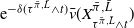 $\mathrm{e}^{-\delta ( {\tau^{\bar{\pi},\bar{L}}\wedge t})}\bar{v}(X^{\bar{\pi},\bar{L}}_{\tau^{\bar{\pi},\bar{L}} \wedge t})$
we can obtain
$\mathrm{e}^{-\delta ( {\tau^{\bar{\pi},\bar{L}}\wedge t})}\bar{v}(X^{\bar{\pi},\bar{L}}_{\tau^{\bar{\pi},\bar{L}} \wedge t})$
we can obtain
 \begin{align}&E_{x}\Big[\mathrm{e}^{-\delta ({\tau^{\bar{\pi},\bar{L}}\wedge t})}\bar{v}\Big(X^{\bar{\pi},\bar{L}}_{\tau^{\bar{\pi},\bar{L}} \wedge t}\Big) -\bar{v}(X_{0-})\Big]\nonumber\\&\quad=E_{x}\bigg[\int^{\tau^{\bar{\pi},\bar{L}} \wedge t}_0\mathrm{e}^{-\delta s}\bigg( \frac{1}{2}\sigma^{2}\big(X^{\bar{\pi},\bar{L}}_{s-}\big) (\bar{\pi}_{s-})^{2}\bar{v}^{\prime\prime}\big(X^{\pi,\bar{L}}_{s-}\big)+\mu\big(X^{\bar{\pi},\bar{L}}_{s-}\big) \bar{\pi}_{s-} \bar{v}^\prime\big(X^{\bar{\pi},\bar{L}}_{s-}\big)-\delta \bar{v}\big(X^{\bar{\pi},\bar{L}}_{s-}\big)\bigg)\,{\mathrm{d}} s\nonumber\\&\quad\quad+\int^{\tau^{\bar{\pi},\bar{L}} \wedge t}_0 \mathrm{e}^{-\delta s}\sigma\big(X^{\bar{\pi},\bar{L}}_{s-}\big) \pi_{s-}\bar{v}\big(X^{\pi,\bar{L}}_{s-}\big) \, {\mathrm{d}} W_s-\int^{\tau^{\bar{\pi},\bar{L}} \wedge t}_0 \mathrm{e}^{-\delta s}\bar{v}^\prime\big(X^{\bar{\pi},\bar{L}}_{s-}\big) \, {\mathrm{d}} \tilde{\bar{L}}_t\nonumber\\ &+\sum_{0\le s \le \tau^{\bar{\pi},\bar{L}} \wedge t} \mathrm{e}^{-\delta s}\big(\bar{v}\big(X^{\bar{\pi},\bar{L}}_{s}\big)- \bar{v}\big(X^{\bar{\pi},\bar{L}}_{s-}\big)\big)\bigg] \nonumber\\ &\quad= E_{x}\bigg[\int^{\tau^{\bar{\pi},\bar{L}} \wedge t}_0\mathrm{e}^{-\delta s}\mathcal{L}_{\bar{v}}(\bar{\pi}_{s-},X^{\bar{\pi},\bar{L}}_{s-}) \, {\mathrm{d}} s\nonumber\\ &\quad\quad+\int^{\tau^{\bar{\pi},\bar{L}} \wedge t}_0 \mathrm{e}^{-\delta s}\sigma\big(X^{\bar{\pi},\bar{L}}_{s-}\big) {\bar{\pi}_{s-}}\bar{v}^\prime\big(X^{,\bar{L}}_{s-}\big) \, {\mathrm{d}} W_s-\int^{\tau^{\bar{\pi},} \wedge t}_0 \mathrm{e}^{-\delta s}\bar{v}^\prime\big(X^{\bar{\pi},\bar{L}}_{s-}\big) \, {\mathrm{d}} \tilde{\bar{L}}_s\nonumber \\ &\quad\quad+\sum_{0\le s \le \tau^{\bar{\pi},\bar{L}} \wedge t} \mathrm{e}^{-\delta s}\big(\bar{v}\big(X^{\bar{\pi},\bar{L}}_{s}\big)-\bar{v}\big(X^{\bar{\pi},\bar{L}}_{s-}\big)\big)\bigg],\end{align}
where $\tilde{\bar{L}}$
represents the continuous part of
$\tilde{\bar{L}}$
represents the continuous part of $\bar{L}$
. Note by (A44) and (A45) we have
$\bar{L}$
. Note by (A44) and (A45) we have $\mathcal{L}_{\bar{v}}(\bar{\pi}_{s-},X^{\bar{\pi},\bar{L}}_{s-})\le 0$
. Note that
$\mathcal{L}_{\bar{v}}(\bar{\pi}_{s-},X^{\bar{\pi},\bar{L}}_{s-})\le 0$
. Note that
 $$\int^{\tau^{\bar{\pi},\bar{L}} \wedge t}_0 \mathrm{e}^{-\delta s}\sigma \big(X^{\bar{\pi},\bar{L}}_{s-}\big) \bar{\pi}_{s-}f\big(X^{\bar{\pi},\bar{L}}_{s-}\big) \, {\mathrm{d}} W_s$$
is a local martingale and so there exists a sequence of stopping times, $\tau_n$
, such that
$\tau_n$
, such that
 $$\int^{\tau^{\bar{\pi},\bar{L}} \wedge t\wedge \tau_n}_0 \mathrm{e}^{-\delta s}\sigma \big(X^{\bar{\pi},\bar{L}}_{s-}\big) \bar{\pi}_{s-}f \big(X^{\bar{\pi},\bar{L}}_{s-}\big)\,{\mathrm{d}} W_s$$
is a martingale. Thus,
 \begin{align}&{\mathrm{E}}_{x}\bigg[\int^{\tau^{\bar{\pi},\bar{L}} \wedge t\wedge \tau_n}_0 \mathrm{e}^{-\delta s}\sigma (X^{\bar{\pi},\bar{L}}_{s-}) \bar{\pi}_{s-}f (X^{\bar{\pi},\bar{L}}_{s-}) \, {\mathrm{d}} W_s\bigg]=0,\quad x\ge 0.\end{align}
As a result, we arrive at
 \begin{align}&E_{x}[\mathrm{e}^{-\delta ({\tau^{\bar{\pi},\bar{L}}\wedge t\wedge \tau_n})}\bar{v}(X^{\bar{\pi},\bar{L}}_{\tau^{\bar{\pi},\bar{L}} \wedge t})] -\bar{v}(x)\nonumber\\&\quad \le -E_{x}\bigg[\int_0^{\tau^{\bar{\pi},\bar{L}}\wedge t\wedge \tau_n} \mathrm{e}^{-\delta s}\bar{v}^\prime(X^{\bar{\pi},\bar{L}}_{s-}){\mathrm{d}} \tilde{\bar{L}}_s\bigg]+ E_{x}\bigg[ \sum_{0\le s \le \tau^{\bar{\pi},\bar{L}}\wedge t\wedge \tau_n} \mathrm{e}^{-\delta s}(\bar{v}(X^{\bar{\pi},\bar{L}}_{s})-\bar{v}(X^{\bar{\pi},\bar{L}}_{s-}))\bigg].\end{align}
Note $E_{x}[\mathrm{e}^{-\delta ({\tau^{\pi,\bar{L}}\wedge t\wedge \tau_n})}\bar{v}(X^{\bar{\pi},\bar{L}}_{\tau^{\bar{\pi},\bar{L}} \wedge t})]\ge0$
. Hence,
$E_{x}[\mathrm{e}^{-\delta ({\tau^{\pi,\bar{L}}\wedge t\wedge \tau_n})}\bar{v}(X^{\bar{\pi},\bar{L}}_{\tau^{\bar{\pi},\bar{L}} \wedge t})]\ge0$
. Hence,
 \begin{align}\bar{v}(x)\ge & E_{x}\bigg[\int_0^{\tau^{\bar{\pi},\bar{L}}\wedge t\wedge \tau_n}\mathrm{e}^{-\delta s}\bar{v}^\prime(X^{\bar{\pi},\bar{L}}_{s-}){\mathrm{d}} \tilde{\bar{L}}_s+ \sum_{0\le s \le \tau^{\bar{\pi},\bar{L}}\wedge t\wedge \tau_n} \mathrm{e}^{-\delta s} (\bar{v}(X^{\bar{\pi},\bar{L}}_{s-})-\bar{v}(X^{\bar{\pi},\bar{L}}_{s}) )\bigg].\end{align}
By letting t and n converge $+\infty$
on both sides and using the monotone convergence we obtain
$+\infty$
on both sides and using the monotone convergence we obtain
 \begin{align}\bar{v}(x)&\ge E_{x}\bigg[\int_0^{\tau^{\bar{\pi},\bar{L}}}\mathrm{e}^{-\delta s}\bar{v}^\prime(X^{\bar{\pi},\bar{L}}_{s-}) \, {\mathrm{d}} \tilde{\bar{L}}_s+ \sum_{0\le s \le \tau^{\bar{\pi},\bar{L}}} \mathrm{e}^{-\delta s} (\bar{v}(X^{\bar{\pi},\bar{L}}_{s-})-\bar{v}(X^{\bar{\pi},\bar{L}}_{s}))\bigg].\end{align}
By letting t and n converge $+\infty$
on both sides and using the monotone convergence we obtain
$+\infty$
on both sides and using the monotone convergence we obtain
 \begin{align}\bar{v}(x)&\ge E_{x}\bigg[\int_0^{\tau^{\bar{\pi},\bar{L}}}\mathrm{e}^{-\delta s}\bar{v}^\prime\big(X^{\bar{\pi},\bar{L}}_{s-}\big) \, {\mathrm{d}} \tilde{\bar{L}}_s+ \sum_{0\le s \le \tau^{\bar{\pi},\bar{L}}} \mathrm{e}^{-\delta s} \big(\bar{v}\big(X^{\bar{\pi},\bar{L}}_{s-}\big)-\bar{v}\big(X^{\bar{\pi},\bar{L}}_{s}\big)\big)\bigg]\end{align}
 \begin{align}& >E_{x}\bigg[\int_0^{\tau^{\bar{\pi},\bar{L}}}\mathrm{e}^{-\delta s} \, {\mathrm{d}} \tilde{\bar{L}}_s+ \sum_{0\le s \le \tau^{\bar{\pi},\bar{L}}\bar{\pi}} \mathrm{e}^{-\delta s}(\bar{L}_{s}-\bar{L}_{s-})\bigg]\end{align}
 \begin{align}&=E_{x}\bigg[\int_0^{\tau^{\bar{\pi},\bar{L}}}\mathrm{e}^{-\delta s}{\mathrm{d}} \bar{L}_s\bigg]=\mathcal{P}(\bar{\pi},\bar{L})(x)>0,\ \ x> 0,\end{align}
where the last inequality holds strictly because $\bar{v}^\prime(x)>1 $
for all
$\bar{v}^\prime(x)>1 $
for all $x>0$
(as has been shown at the beginning of the proof to (iii)) and
$x>0$
(as has been shown at the beginning of the proof to (iii)) and
 \begin{align*}&E_{x}\bigg[\int_0^{\tau^{\bar{\pi},\bar{L}}}\mathrm{e}^{-\delta s}\,{\mathrm{d}} \tilde{\bar{L}}_s+ \sum_{0\le s \le \tau^{\bar{\pi},\bar{L}}} \mathrm{e}^{-\delta s}(X_{s-}^{\bar{\pi},\bar{L}}-X_{s}^{\bar{\pi},\bar{L}})\bigg]\nonumber\\&\quad =E_{x}\bigg[\int_0^{\tau^{\bar{\pi},\bar{L}}}\mathrm{e}^{-\delta s}\,{\mathrm{d}} \tilde{\bar{L}}_s+ \sum_{0\le s \le \tau^{\bar{\pi},\bar{L}}} \mathrm{e}^{-\delta s}(\bar{L}_{s}-\bar{L}_{s-})\bigg]>0\end{align*}
(as can be seen from (A58) and (A59)). Note that $\bar{v}(x)=\lim_{b\rightarrow +\infty} v_b(x)\le V(x)$
, which combined with (A59) implies
$\bar{v}(x)=\lim_{b\rightarrow +\infty} v_b(x)\le V(x)$
, which combined with (A59) implies $V(x)\ge \bar{v}(x)>\mathcal{P}(\bar{\pi},\bar{L})(x)$
for
$V(x)\ge \bar{v}(x)>\mathcal{P}(\bar{\pi},\bar{L})(x)$
for $x>0$
. This contradicts the defining property of
$x>0$
. This contradicts the defining property of $(\bar{\pi},\bar{L})$
:
$(\bar{\pi},\bar{L})$
: $V(\bar{\pi}, \bar{L})(x)=V(x)$
.
$V(\bar{\pi}, \bar{L})(x)=V(x)$
.
A.11. Proof of Theorem 6
Define $f(x)=x$
. We can observe that under
$f(x)=x$
. We can observe that under $L^0$
, the company pays out all the initial wealth at time 0 and claims bankruptcy. Thus,
$L^0$
, the company pays out all the initial wealth at time 0 and claims bankruptcy. Thus, $\mathcal{P}(\pi^0, L^0)(x)=x=f(x)$
for
$\mathcal{P}(\pi^0, L^0)(x)=x=f(x)$
for $x\ge 0$
. Therefore,
$x\ge 0$
. Therefore, $f(x)=x\le \sup_{(\pi,L)\in\mathcal{A}}\mathcal{P}(\pi, L)(x)=V(x)$
for
$f(x)=x\le \sup_{(\pi,L)\in\mathcal{A}}\mathcal{P}(\pi, L)(x)=V(x)$
for $x\ge 0$
. Thus, it is sufficient to show
$x\ge 0$
. Thus, it is sufficient to show $f(x)\ge V(x)$
. Note
$f(x)\ge V(x)$
. Note $\mu(0)\le 0$
,
$\mu(0)\le 0$
, $f(x)=x$
,
$f(x)=x$
, $f^\prime(x)=1$
,
$f^\prime(x)=1$
, $f^{\prime\prime}(x)=0$
, and
$f^{\prime\prime}(x)=0$
, and $\mu^\prime(x)\le \delta$
, we can easily obtain
$\mu^\prime(x)\le \delta$
, we can easily obtain
 \begin{align*} &\max_{a\in[0,1]}\left(\frac{1}{2}\sigma^{2}(x) a^{2}\,f^{\prime\prime}(x)+\mu(x) a\,f^\prime(x)-\delta\,f(x)\right)=\mu(x)-\delta x\le \mu(0)+\delta x -\delta x \le 0,\quad x\ge 0,\\ &f^\prime(x)=1,\quad x\ge 0.\end{align*}
Further note $f(0)=0$
and f(x) is sufficiently smooth. Thus, all the conditions in Theorem 1 are fulfilled and, thus, by Theorem 1 we can conclude
$f(0)=0$
and f(x) is sufficiently smooth. Thus, all the conditions in Theorem 1 are fulfilled and, thus, by Theorem 1 we can conclude $f(x)\ge V(x)$
. Consequently,
$f(x)\ge V(x)$
. Consequently, $f(x)=V(x)$
and
$f(x)=V(x)$
and $\mathcal{P}(\pi^0,L^0)=f(x)=V(x)$
for
$\mathcal{P}(\pi^0,L^0)=f(x)=V(x)$
for $x\ge 0$
.
$x\ge 0$
.
A.12. Proof of Lemma 7
Recall that we are considering the case $\mu(0)> 0$
and in this case
$\mu(0)> 0$
and in this case $\mu(x)>0$
for
$\mu(x)>0$
for $0\le x < x_0$
and
$0\le x < x_0$
and $\mu(x_0)=0$
. Note from (26)
$\mu(x_0)=0$
. Note from (26) $A(0)=0$
and
$A(0)=0$
and
 $$\lim_{x\rightarrow x_0}A(x)=\lim_{x\rightarrow x_0}\frac{\int_{0}^{x}(2\delta+\frac{\mu^{2}(y)}{\sigma^{2}(y)})\mathrm{d} y}{\mu(x)}=\infty.$$
Hence, by its continuity we know that A(x) attains 1 for some $x\in(0,x_0))$
, which implies that
$x\in(0,x_0))$
, which implies that $x^*$
, which is the smallest positive point at which A(x) attains 1, is between 0 and
$x^*$
, which is the smallest positive point at which A(x) attains 1, is between 0 and $x_0$
. From (26) it follows that
$x_0$
. From (26) it follows that
 $$A(x)\geq \frac{\int_{0}^{x}2\delta dy}{\mu(x)}=\frac{2\delta x}{\mu(x)}\geq \frac{2\delta x}{\mu(0)+\delta x}>1 \quad \mbox{for } x>\frac{\mu(0)}{\delta},$$
where the second to the last inequality is due to $\mu^\prime (x)\leq\delta$
. Thus, A(x) attains 1 at or before
$\mu^\prime (x)\leq\delta$
. Thus, A(x) attains 1 at or before ${\mu(0)}/{\delta}$
, that is,
${\mu(0)}/{\delta}$
, that is, $x\le {\mu(0)}/{\delta}$
.
$x\le {\mu(0)}/{\delta}$
.
We can follow the same steps as in the proof of Lemma 1 to show that A(x) is increasing on $[0,x^*]$
.
$[0,x^*]$
.
A.13. Proof of Lemma 8
All the steps in the proof of Lemma 3 leading to (A37) remain valid for any x, yielding
 \begin{align} g^{\prime\prime}_{1}(x)+g^{\prime\prime}_{2}(x)\int_{0}^{x}\mathrm{e}^{\int_{z}^{x}\frac{\mu(y)}{\sigma^{2}(y)A(y)}\,\mathrm{d} y}\,\mathrm{d} z=-\frac{\mu(x)}{\sigma^{2}(x)A(x)}.\end{align}
Now, note that $x^* < x_0$
(by Lemma 7) and, hence, it follows from (57) that
$x^* < x_0$
(by Lemma 7) and, hence, it follows from (57) that $\mu(x^*)>0$
. Further note that
$\mu(x^*)>0$
. Further note that $ A(x^*)=1$
(by Lemma 7). Therefore,
$ A(x^*)=1$
(by Lemma 7). Therefore,
 $$g^{\prime\prime}_{1}(x^*)+g^{\prime\prime}_{2}(x^*)\int_{0}^{x^{*}}\mathrm{e}^{\int_{z}^{x^*}\frac{\mu(y)}{\sigma^{2}(y)A(y)}\,\mathrm{d} y}\,\mathrm{d} z<0,$$
which, along with the definition for $b^*$
in (48), implies that
$b^*$
in (48), implies that $b^*>x^*$
.
$b^*>x^*$
.
As $\mu(x_0)=0$
, it follows from (A60) that
$\mu(x_0)=0$
, it follows from (A60) that
 $$g^{\prime\prime}_{1}(x_0)+g^{\prime\prime}_{2}(x_0)\int_{0}^{x_0}\mathrm{e}^{\int_{z}^{x_0}\frac{\mu(y)}{\sigma^{2}(y)A(y)}\,\mathrm{d} y}\,\mathrm{d} z=-\frac{\mu(x_0)}{\sigma^{2}(x_0)A(x_0)}=0,$$
which, along with the definition for $b^*$
in (48), implies that
$b^*$
in (48), implies that $b^*\le x_0$
.
$b^*\le x_0$
.
A.14. Proof of Theorem 7
It follows from Lemma 8 that $\mu(x) > 0$
for
$\mu(x) > 0$
for $0 \le x < b^*$
. In light of the results in Lemma 7, we observe that the proofs of Theorems 2–4 remain valid and, therefore, these theorems still hold in this case. As a result, all the steps in the proof of Theorem 4 continue to apply. This completes the proof.
$0 \le x < b^*$
. In light of the results in Lemma 7, we observe that the proofs of Theorems 2–4 remain valid and, therefore, these theorems still hold in this case. As a result, all the steps in the proof of Theorem 4 continue to apply. This completes the proof.
A.15. Proof of Equation (83)
Recall that $V^{\alpha,\beta}$
represents the value function in [Reference Choulli, Taksar and Zhou10] and it has the following representation:
$V^{\alpha,\beta}$
represents the value function in [Reference Choulli, Taksar and Zhou10] and it has the following representation:
 \begin{equation}V^{\alpha,\beta}(x)=\begin{cases}k_{1}(\alpha, \beta)(\mathrm{e}^{r_{+}(\alpha) x}-\mathrm{e}^{r_{-}(\alpha) x}), \quad & x\in[0,x_{\alpha}], \\[4pt] \displaystyle \frac{\mu \alpha}{2 \gamma} (V^{\alpha,\beta})^{\prime}(x_{\alpha}-)\left(\frac{x-x_{\alpha}+y_{\alpha}}{y_{\alpha}}\right)^{1-\Gamma},\quad & x\in(x_{\alpha},x_{\beta}), \\[4pt] k_{1}(\beta) \mathrm{e}^{r_{+}(\beta)(x-x_{1})}+k_{2}(\beta) \mathrm{e}^{r_{-}(\beta)(x-x_{1})},\quad & x\in[x_{\beta},x_{1}), \\[4pt] k_{1}(\beta)+k_{2}(\beta)+x-x_{1}, & x\in[x_{1},\infty), \end{cases}\end{equation}
where $\gamma>0$
is the discount rate,
$\gamma>0$
is the discount rate,
 \begin{align}r_{+}(\alpha)&=\frac{-\mu+[\mu^2+2 \sigma^2 \gamma]^{1 / 2}}{\alpha \sigma^2},\quad r_{-}(\alpha)=\frac{-\mu-[\mu^2+2 \sigma^2 \gamma]^{1 / 2}}{\alpha \sigma^2},\nonumber\\r_{+}(\beta)&=\frac{-\mu+[\mu^2+2 \sigma^2 \gamma]^{1 / 2}}{\beta \sigma^2},\quad r_{-}(\beta)=\frac{-\mu-[\mu^2+2 \sigma^2 \gamma]^{1 / 2}}{\beta \sigma^2},\nonumber\\x_\alpha &=\frac{1}{r_{+}(\alpha)-r_{-}(\alpha)} \ln \left(-\frac{r_{-}(\alpha)}{r_{+}(\alpha)}\right)>0,\quad x_\beta=\frac{\mu \sigma^2}{\mu^2+2 \sigma^2 \gamma}(\beta-\alpha)+x_\alpha,\nonumber\\y_\alpha &= \frac{\mu \sigma^2 \alpha}{\mu^2+2 \sigma^2 \gamma},\quad\Gamma = \frac{\mu^2}{\mu^2+2 \sigma^2 \gamma},\nonumber\\x_1&=x_\beta-\Delta,\quad \Delta=\frac{\beta \sigma^2}{2[\mu^2+2 \sigma^2 \gamma]^{1 / 2}} \log \left(\frac{-\mu+[\mu^2+2 \sigma^2 \gamma]^{1 / 2}}{\mu+[\mu^2+2 \sigma^2 \gamma]^{1 / 2}}\right)<0,\nonumber\\k_1(\beta)&=\frac{-r_{-}(\beta)}{r_{+}(\beta)(r_{+}(\beta)-r_{-}(\beta))},\quad k_2(\beta)=\frac{r_{+}(\beta)}{r_{-}(\beta)(r_{+}(\beta)-r_{-}(\beta))},\end{align}
and
 \begin{equation}k_1(\alpha, \beta)=\frac{k_1(\beta) r_{+}(\beta) \mathrm{e}^{r_{+}(\beta) \Delta}+k_2(\beta) r_{-}(\beta) \mathrm{e}^{r_{-}(\beta) \Delta}}{\frac{\alpha \mu}{2 \gamma y_\alpha} (r_{+}(\alpha) \mathrm{e}^{r_{+}(\alpha) x_\alpha}-r_{-}(\alpha) \mathrm{e}^{r_{-}(\alpha) x_\alpha})\left(\frac{\beta}{\alpha}\right)^{-\Gamma}(1-\Gamma)}.\end{equation}
In the original form of the formulas for $V^{\alpha,\beta}$
, the formulas for the second piece use
$V^{\alpha,\beta}$
, the formulas for the second piece use $(V^{\alpha,\beta})^{\prime}(x_{\alpha})$
, which we think should be
$(V^{\alpha,\beta})^{\prime}(x_{\alpha})$
, which we think should be $(V^{\alpha,\beta})^{\prime}(x_{\alpha}-)$
. The two quantities are eventually same as
$(V^{\alpha,\beta})^{\prime}(x_{\alpha}-)$
. The two quantities are eventually same as $V^{\alpha,\beta}$
is continuously differentiable at
$V^{\alpha,\beta}$
is continuously differentiable at $x_{\alpha}$
. By direct calculation using the first piece of the formulas for
$x_{\alpha}$
. By direct calculation using the first piece of the formulas for $(V^{\alpha,\beta})^{\prime}$
we obtain
$(V^{\alpha,\beta})^{\prime}$
we obtain
 \begin{align}\frac{\mu\alpha}{2\gamma} (V^{\alpha, \beta})^{\prime}(x_\alpha-)&=\frac{\mu\alpha}{2\gamma} k_1(\alpha, \beta)(r_{+}(\alpha) \mathrm{e}^{r_{+}(\alpha) x_\alpha}-r_{-}(\alpha) \mathrm{e}^{r_{-}(\alpha) x_\alpha})\nonumber\\&={y_\alpha}\left(\frac{ \beta}{\alpha}\right)^{\Gamma}\frac{k_1(\beta) r_{+}(\beta) \mathrm{e}^{r_{+}(\beta) \Delta}+k_2(\beta) r_{-}(\beta) \mathrm{e}^{r_{-}(\beta) \Delta}}{(1-\Gamma)},\end{align}
where the last equality follows immediately by plugging in (A63). Therefore, the second piece of formulas in (A61), which is the formula of $V^{\alpha, \beta}(x)$
for
$V^{\alpha, \beta}(x)$
for $x_{\alpha} \leq x < x_{\beta}$
, becomes
$x_{\alpha} \leq x < x_{\beta}$
, becomes
 \begin{align} &V^{\alpha,\beta}(x)\nonumber \\&={y_\alpha}\left(\frac{ \beta}{\alpha}\right)^{\Gamma}\frac{k_1(\beta) r_{+}(\beta) e^{r_{+}(\beta) \Delta}+k_2(\beta) r_{-}(\beta) \mathrm{e}^{r_{-}(\beta) \Delta}}{(1-\Gamma)}\left(\frac{x-x_{\alpha}+y_{\alpha}}{y_{\alpha}}\right)^{1-\Gamma}\nonumber\\ &=\frac{\mu \sigma^2 \alpha}{\mu^2+2 \sigma^2 \gamma}\left(\frac{ \beta}{\alpha}\right)^{\Gamma}\frac{k_1(\beta) r_{+}(\beta) \mathrm{e}^{r_{+}(\beta) \Delta}+k_2(\beta) r_{-}(\beta) \mathrm{e}^{r_{-}(\beta) \Delta}}{(1-\Gamma)}\left(\frac{x-x_{\alpha}+\frac{\mu \sigma^2 \alpha}{\mu^2+2 \sigma^2 \gamma}}{\frac{\mu \sigma^2 \alpha}{\mu^2+2 \sigma^2 \gamma}}\right)^{1-\Gamma}\nonumber\\ &=\left(k_1(\beta) r_{+}(\beta) \mathrm{e}^{r_{+}(\beta) \Delta}+k_2(\beta) r_{-}(\beta) \mathrm{e}^{r_{-}(\beta) \Delta}\right)\frac{\mu {\beta}^{\Gamma}}{2\gamma}\left(\frac{x-x_{\alpha}+\frac{\mu \sigma^2 \alpha}{\mu^2+2 \sigma^2 \gamma}}{\frac{\mu \sigma^2}{\mu^2+2 \sigma^2 \gamma}}\right)^{1-\Gamma}.\end{align}
When $\alpha=0,\beta=1$
, by noting
$\alpha=0,\beta=1$
, by noting $\gamma=\delta$
(because
$\gamma=\delta$
(because $\gamma$
and
$\gamma$
and $\delta$
represent the same thing, the discount rate, in the reference [Reference Choulli, Taksar and Zhou10] and this paper, respectively), from the above equations we can conclude
$\delta$
represent the same thing, the discount rate, in the reference [Reference Choulli, Taksar and Zhou10] and this paper, respectively), from the above equations we can conclude $x_\alpha=0$
,
$x_\alpha=0$
, $ x_\beta= {\mu \sigma^2}/({\mu^2+2 \sigma^2 \delta})=x^*,$ $y_\alpha=0$
,
$y_\alpha=0$
, $r_{+}(1)=\theta_1$
, and
$r_{+}(1)=\theta_1$
, and $r_{-}(1)=\theta_2$
. Using these and noting
$r_{-}(1)=\theta_2$
. Using these and noting $\gamma=\delta$
again, we can obtain that when
$\gamma=\delta$
again, we can obtain that when $\alpha=0$
and
$\alpha=0$
and $\beta=1$
,
$\beta=1$
,
 \begin{align} k_1(1)&=\frac{-\theta_2}{\theta_1 (\theta_1-\theta_2)}, \quad k_2(1)=\frac{\theta_1}{\theta_2 (\theta_1-\theta_2)}, \end{align}
 \begin{align} x_1&=x_\beta-\Delta=x_\beta-\frac{ \sigma^2}{2 [\mu^2+2 \sigma^2 \delta ]^{1 / 2}} \ln \left(\frac{-\mu+[\mu^2+2 \sigma^2 \delta]^{1 / 2}}{\mu+[\mu^2+2 \sigma^2 \delta]^{1 / 2}}\right)\nonumber\\ &=x^*+\frac{\ln\left(-\frac{\theta_2}{\theta_1}\right)}{\theta_1-\theta_2}=x^*+ \frac{\ln\frac{\theta_2^2(1-\theta_1\frac{\mu}{2\delta})}{\theta_1^2(1-\theta_2 \frac{\mu}{2\delta})}}{\theta_1-\theta_2}=b^*,\end{align}
where the last equality follows from (79). Recall $\Gamma = {\mu^2}/({\mu^2+2 \sigma^2 \gamma})$
and
$\Gamma = {\mu^2}/({\mu^2+2 \sigma^2 \gamma})$
and $\gamma=\delta$
. Substituting these, (A65), (A66),
$\gamma=\delta$
. Substituting these, (A65), (A66), $x_{\beta=1}=x^*$
, and
$x_{\beta=1}=x^*$
, and $x_1=b^*$
into (A61) we have
$x_1=b^*$
into (A61) we have
 \begin{equation*}V^{\alpha=0,\beta=1}(x)=\begin{cases} \left(\frac{-\theta_2}{(\theta_1-\theta_2)} \mathrm{e}^{\theta_1 \Delta}+\frac{\theta_1}{(\theta_1-\theta_2)} \mathrm{e}^{\theta_2 \Delta}\right)\frac{\mu}{2\delta}\left(\frac{x}{x^*}\right)^{1-\Gamma},\quad & x\in[0,x^*),\\k_{1}(1) \mathrm{e}^{\theta_1 (x-x^* )}+k_2(1) \mathrm{e}^{\theta_2(x-x^*)},\quad & x\in[x^*,b^*),\\k_{1}(1)+k_{2}(1)+x-b^*, & x\in[b^*,\infty).\end{cases}\end{equation*}
Funding information
This work was supported by General Project of Humanities and Social Sciences Research of Ministry of Education (grant number 24YJAZH197) and National Natural Science Foundation of China (grant number 11801265).
Competing interests
There were no competing interests to declare which arose during the preparation or publication process of this article.