





1. Introduction
Impacts between droplets and solid surfaces can commonly cause erosion problems in engineering applications, including aircraft surface erosion (Gohardani Reference Gohardani2011), wind turbine blade leading-edge erosion (LEE, Herring et al. Reference Herring, Dyer, Martin and Ward2019) and steam turbine blade erosion (Preece & Brunton Reference Preece and Brunton1980). Especially at high-speed impacts, cavitation could happen simultaneously inside the droplet and the collapse of cavitation bubbles induces further shock waves that may damage the surface material (Field, Dear & Ogren Reference Field, Dear and Ogren1989; Gonzalez-Avila, Zeng & Ohl Reference Gonzalez-Avila, Zeng and Ohl2024).
The extreme compressible flows generated during the impact of high-speed droplets have been widely studied and discussed. Upon impact, an intense water-hammer (WH) shock wave forms and begins to propagate almost instantaneously. The resulting high post-shock pressure – commonly referred to as the WH pressure – is recognised as a primary damage mechanism to the solid wall (Cook Reference Cook1928; Bowden & Field Reference Bowden and Field1964; Heymann Reference Heymann1969; Lesser & Field Reference Lesser and Field1983; Haller et al. Reference Haller, Ventikos, Poulikakos and Monkewitz2002). This initial transient WH pressure is estimated ( $p_{\textit{WH}}=\rho _lU_0(c_l+\chi U_0)$
, where
$p_{\textit{WH}}=\rho _lU_0(c_l+\chi U_0)$
, where $\rho _l$
and
$\rho _l$
and $c_l$
are the density and sound speed of the undisturbed liquid, respectively, and
$c_l$
are the density and sound speed of the undisturbed liquid, respectively, and $\chi$
is a constant) to be proportional to the droplet’s impact velocity,
$\chi$
is a constant) to be proportional to the droplet’s impact velocity, $U_0$
, and the acoustic impedance of the liquid (Heymann Reference Heymann1969). For example, when a water droplet impacts a rigid wall at a velocity of
$U_0$
, and the acoustic impedance of the liquid (Heymann Reference Heymann1969). For example, when a water droplet impacts a rigid wall at a velocity of $U_0\sim 50$ $\mathrm{m\,s^{-1}}$
, the resulting WH pressure can reach approximately
$\mathrm{m\,s^{-1}}$
, the resulting WH pressure can reach approximately $75$
$75$ $\mathrm{MPa}$
. In addition to the pressure spike, the impact generates high-speed lateral liquid jets (Lesser & Field Reference Lesser and Field1983; Field et al. Reference Field, Dear and Ogren1989; Haller et al. Reference Haller, Ventikos, Poulikakos and Monkewitz2002), believed to form when the WH shock wave detaches from the wall. These jets can attain velocities significantly greater than the initial impact velocity. According to experimental data from Field et al. (Reference Field, Dear and Ogren1989), a droplet impact at
$\mathrm{MPa}$
. In addition to the pressure spike, the impact generates high-speed lateral liquid jets (Lesser & Field Reference Lesser and Field1983; Field et al. Reference Field, Dear and Ogren1989; Haller et al. Reference Haller, Ventikos, Poulikakos and Monkewitz2002), believed to form when the WH shock wave detaches from the wall. These jets can attain velocities significantly greater than the initial impact velocity. According to experimental data from Field et al. (Reference Field, Dear and Ogren1989), a droplet impact at $U_0=110$ $\mathrm{m\,s^{-1}}$
produces lateral jets with velocities of the order of
$\mathrm{m\,s^{-1}}$
produces lateral jets with velocities of the order of ${O}(10^3 \mathrm{m\,s^{-1}})$
. The presence of such high pressure and high liquid velocities within the droplet far exceed those predicted by Bernoulli fields, as described in our previous work on inviscid potential-flow solutions for droplet impact (Hao et al. Reference Hao, Charalambides, Hardalupas, Sergis and Taylor2026b
). At such extreme speeds, these jets exert intense shear forces on the wall, contributing to additional material damage (Kondo & Ando Reference Kondo and Ando2019). Furthermore, liquid cavitation inside the droplet and the subsequent collapse of vapour bubbles are also considered key erosion mechanisms. Cavitation within the droplet is triggered by large pressure fluctuations resulting from the propagation and multiple reflections of the WH shock wave. This phenomenon has been observed in experiments (Lesser & Field Reference Lesser and Field1983; Field et al. Reference Field, Dear and Ogren1989, Reference Field, Camus, Tinguely and Obreschkow2012; Gonzalez-Avila et al. Reference Gonzalez-Avila, Zeng and Ohl2024) and analysed through numerical simulations (Sanada, Ando & Colonius Reference Sanada, Ando and Colonius2011; Kondo & Ando Reference Kondo and Ando2016; Wu et al. Reference Wu, Xiang and Wang2018, Reference Wu, Liu and Wang2021). The experiments by Field et al. (Reference Field, Dear and Ogren1989) clearly showed that reflections of the shock wave from the droplet’s internal surface generate rarefaction waves that focus within the two-dimensional droplet, leading to localised cavitation. Similar behaviour has also been observed in three-dimensional configurations (Gonzalez-Avila et al. Reference Gonzalez-Avila, Zeng and Ohl2024). Wu, Xiang & Wang (Reference Wu, Xiang and Wang2018) provided a detailed analysis of this cavitation mechanism using ray theory and simulations, identifying the theoretical location of the cavitation zone. Wu, Liu & Wang (Reference Wu, Liu and Wang2021) further highlighted the influence of the solid wall’s geometry on the cavitation dynamics. Once cavitation is initiated, the collapse of vapour bubbles – especially those near the solid wall – produces intense shock waves and secondary liquid jets (Field et al. Reference Field, Camus, Tinguely and Obreschkow2012; Zeng et al. Reference Zeng, Gonzalez-Avila, Voorde and Ohl2018; Wu et al. Reference Wu, Liu and Wang2021), which can impose significant stresses on the wall and result in material damage (Zeng, An & Ohl Reference Zeng, An and Ohl2022; Dular & Ohl Reference Dular and Ohl2023; Reese, Ohl & Ohl Reference Reese, Ohl and Ohl2023).
${O}(10^3 \mathrm{m\,s^{-1}})$
. The presence of such high pressure and high liquid velocities within the droplet far exceed those predicted by Bernoulli fields, as described in our previous work on inviscid potential-flow solutions for droplet impact (Hao et al. Reference Hao, Charalambides, Hardalupas, Sergis and Taylor2026b
). At such extreme speeds, these jets exert intense shear forces on the wall, contributing to additional material damage (Kondo & Ando Reference Kondo and Ando2019). Furthermore, liquid cavitation inside the droplet and the subsequent collapse of vapour bubbles are also considered key erosion mechanisms. Cavitation within the droplet is triggered by large pressure fluctuations resulting from the propagation and multiple reflections of the WH shock wave. This phenomenon has been observed in experiments (Lesser & Field Reference Lesser and Field1983; Field et al. Reference Field, Dear and Ogren1989, Reference Field, Camus, Tinguely and Obreschkow2012; Gonzalez-Avila et al. Reference Gonzalez-Avila, Zeng and Ohl2024) and analysed through numerical simulations (Sanada, Ando & Colonius Reference Sanada, Ando and Colonius2011; Kondo & Ando Reference Kondo and Ando2016; Wu et al. Reference Wu, Xiang and Wang2018, Reference Wu, Liu and Wang2021). The experiments by Field et al. (Reference Field, Dear and Ogren1989) clearly showed that reflections of the shock wave from the droplet’s internal surface generate rarefaction waves that focus within the two-dimensional droplet, leading to localised cavitation. Similar behaviour has also been observed in three-dimensional configurations (Gonzalez-Avila et al. Reference Gonzalez-Avila, Zeng and Ohl2024). Wu, Xiang & Wang (Reference Wu, Xiang and Wang2018) provided a detailed analysis of this cavitation mechanism using ray theory and simulations, identifying the theoretical location of the cavitation zone. Wu, Liu & Wang (Reference Wu, Liu and Wang2021) further highlighted the influence of the solid wall’s geometry on the cavitation dynamics. Once cavitation is initiated, the collapse of vapour bubbles – especially those near the solid wall – produces intense shock waves and secondary liquid jets (Field et al. Reference Field, Camus, Tinguely and Obreschkow2012; Zeng et al. Reference Zeng, Gonzalez-Avila, Voorde and Ohl2018; Wu et al. Reference Wu, Liu and Wang2021), which can impose significant stresses on the wall and result in material damage (Zeng, An & Ohl Reference Zeng, An and Ohl2022; Dular & Ohl Reference Dular and Ohl2023; Reese, Ohl & Ohl Reference Reese, Ohl and Ohl2023).
While the collapse of cavitation bubbles is recognised as a potential source of material damage, due to the rapid attenuation of the induced shock waves with distance, their effects are highly localised, and the damage is mainly caused by vapour bubbles close to the wall surface (Blake & Gibson Reference Blake and Gibson1987). As a result, most cavitation-induced erosion is driven by fatigue damage, with only a few cases of erosion caused by the collapse of a single vapour bubble (Brennen Reference Brennen2015). In many engineering applications, erosion due to droplet impact and cavitation is often considered and treated the same, as both mechanisms primarily involve shock waves and liquid jets (Cook Reference Cook1928), resulting in similar erosion appearance, such as pits and craters, on the material surface (Bowden & Field Reference Bowden and Field1964). Preece & Brunton (Reference Preece and Brunton1980) studied jet and cavitation erosion on metals and alloys, finding a strong correlation between the two failure modes, with the shear stress from jet impacts being more pronounced in the erosion of ductile materials. In terms of material properties, Mann & Arya (Reference Mann and Arya2002) highlighted the critical role of fatigue strength in cavitation resistance, given the high frequency of shock waves generated by cavity collapse (Chaplin Reference Chaplin2019). While much of the literature has focused on fatigue erosion, Xu et al. (Reference Xu, Wang, Qin, Chen and Chen2010) demonstrated that a single vapour bubble can cause material surface damage. In their experiments, droplets of distilled water (figure 1 a) and water infused with nano-particles as cavitation nuclei (figure 1 b) were used to bombard material surfaces. The latter produced round, overlapping craters in addition to scratches from the nano-particles, indicating that damage can indeed be caused by individual vapour collapses. Despite these findings, most studies on cavitation damage have concentrated on metals and alloys, particularly in aviation and steam turbine applications, with limited research on composite materials and the effects of cavitation on their erosion behaviour. These findings underscore the necessity for continued investigation into the erosive potential of cavitation, especially in the context of composite systems.
There are several mechanisms behind droplet impact and cavitation erosion, among which two distinct ‘ring patterns’ are most pronounced for different material types (Hancox & Brunton Reference Hancox and Brunton1966). For ductile materials with low compressive but high tensile strength, pits typically form due to plastic deformation caused by the penetrating jet (Bourne & Field Reference Bourne and Field1995). The shearing or tearing of the droplet’s outward flows may also generate craters (i.e. an inner ring) (Hancox & Brunton Reference Hancox and Brunton1966). In particular, surface damage is more easily initiated at local weak spots on the material surface (Thomas Reference Thomas1966). In contrast, for brittle materials with high compressive but low tensile strengths, ring-pattern cracks (i.e. outer ring) can form due to interactions of tensile waves, including the well-known Rayleigh surface wave (Miller & Pursey Reference Miller and Pursey1955; Blowers Reference Blowers1969). These waves are most intense at the periphery (Hancox & Brunton Reference Hancox and Brunton1966; Bourne & Field Reference Bourne and Field1995) of the loaded area. In the specific context of LEE induced by raindrop impacts on wind turbine blades (figure 1 c–e), fatigue has traditionally been considered the primary damage mechanism (Springer Reference Springer1976; Ibrahim & Medraj Reference Ibrahim and Medraj2020) due to the repeated nature of raindrop impacts. Micron-sized pits, similar in size to those induced by cavitation in similar engineering applications (Xu et al. Reference Xu, Wang, Qin, Chen and Chen2010; Azar, Yelkarasi & Ürgen Reference Azar, Yelkarasi and Ürgen2017; Ma et al. Reference Ma, Harvey, Wellman and Wood2018), have been observed on the surfaces of test samples (Tobin et al. Reference Tobin, Young, Raps and Rohr2011; O’carroll et al. Reference O’carroll, Hardiman, Tobin and Young2018; Sanchez et al. Reference Sanchez, Hao, Domenech, Hardalupas, Dyer, Garcia, Charalambides, Ibanez-Arnal, Sergis and Taylor2026), as well as in field conditions (Rasool, Middleton & Stack Reference Rasool, Middleton and Stack2020; Doagou-Rad & Mishnaevsky Reference Doagou-Rad and Mishnaevsky2020; Hoksbergen, Baran & Akkerman Reference Hoksbergen, Baran and Akkerman2020). Additionally, indirect erosion may occur due to delamination at the interfaces between material layers (Sánchez et al. Reference Sánchez, Olivares, Domenech and Cortés2020), caused by shearing motion of the impact (Ibrahim & Medraj Reference Ibrahim and Medraj2020). This could lead to non-structural matrix cracking, interface debonding and ultimately fibre failure in composite blade materials (Mishnaevsky Reference Mishnaevsky2019; Eder, Sarhadi & Chen Reference Eder, Sarhadi and Chen2021). Together, these findings highlight the complex, material-dependent nature of impact and cavitation erosion mechanisms.
Experimental results of the eroded surface after being impacted by the water steam at $60$
$60$ $\mathrm{m\,s^{-1}}$
(Xu et al. Reference Xu, Wang, Qin, Chen and Chen2010): (
$\mathrm{m\,s^{-1}}$
(Xu et al. Reference Xu, Wang, Qin, Chen and Chen2010): ( $a$
) no damage with distilled water, (
$a$
) no damage with distilled water, ( $b$
) cavitation erosion with nano-particle-infused water. Examples of LEE on wind blades across a range of years in service (Keegan, Nash & Stack Reference Keegan, Nash and Stack2013): (
$b$
) cavitation erosion with nano-particle-infused water. Examples of LEE on wind blades across a range of years in service (Keegan, Nash & Stack Reference Keegan, Nash and Stack2013): ( $c$
)
$c$
) $1$
year; (
$1$
year; ( $d$
)
$d$
) $2$
years, and (
$2$
years, and ( $e$
)
$e$
) $10+$
years.
$10+$
years.

While most of the literature addresses the fluid and material phases of erosion problems separately, several notable studies have investigated the complex problem of fluid–structure interaction (FSI). Experimentally, Sun et al. (Reference Sun, Alvarez-Novoa, Andrade, Gutierrez, Gordillo and Cheng2022) developed a high-speed stress microscopy technique by combining traction force microscopy, laser-sheet microscopy and high-speed photography. This approach enables the capture of rapid droplet impact dynamics and the simultaneous mapping of pressure and stress fields within the underlying material during impact events. Similarly, Yokoyama et al. (Reference Yokoyama, Mitchell, Nassiri, Kinsey, Korkolis and Tagawa2023) employed integrated photoelasticity to reconstruct three-dimensional stress fields in soft materials. However, both techniques are limited to optically transparent and soft materials (of stiffness of the order O( $\mathrm{kPa}$
)), and to low-speed impacts (of the order O(
$\mathrm{kPa}$
)), and to low-speed impacts (of the order O( $1$
$1$ $\mathrm{m\,s^{-1}}$
)) below the cavitation threshold. Reese et al. (Reference Reese, Ohl and Ohl2023) experimentally investigated tangential stresses on an elastic surface induced by cavitation bubble collapse by tracking the displacements of embedded particles on the surface. Yet, this method is restricted to surface measurements. Consequently, experimental techniques are generally unsuitable for studying droplet impact erosion in blade materials. Numerical FSI studies of erosion problems typically use finite-element (FE) methods (Keegan, Nash & Stack Reference Keegan, Nash and Stack2012), including smoothed particle hydrodynamics and coupled Eulerian–Lagrangian approaches. However, FE methods often suffer from limited resolution of the liquid phase, or require prohibitively high computational resources, due to the large deformations involved in the liquid phase (Zhou et al. Reference Zhou, Li, Chen, Xu, Hui and Zhang2009). An alternative approach, implemented by Amirzadeh et al. (Reference Amirzadeh, Louhghalam, Raessi and Tootkaboni2017), and more recently by Hoksbergen, Akkerman & Baran (Reference Hoksbergen, Akkerman and Baran2023), involves coupling an independent computational fluid dynamics simulation of the liquid phase with an FE analysis of the solid phase. Their studies achieved notable success in capturing both fluid dynamics and material response. In a previous series of studies, the present authors were able to couple an analytical solution for droplet impact (Hao et al. Reference Hao, Charalambides, Hardalupas, Sergis and Taylor2026b
) with an FE material analysis. This approach achieved improved accuracy while greatly reducing computational time by up to 97 % (Hao et al. Reference Hao, Charalambides, Hardalupas, Sergis and Taylor2026a
). Other advanced FSI simulations in related fields – though not specifically on droplet impact erosion – include multiphase bubble–liquid–solid models (Zeng et al. Reference Zeng, An and Ohl2022; Reese et al. Reference Reese, Ohl and Ohl2023; Heidary, Ohl & Mojra Reference Heidary, Ohl and Mojra2024). However, no existing numerical study has yet incorporated phase change and cavitation phenomena into FSI simulations, which generally require higher spatiotemporal resolution than those addressing impact events alone.
$\mathrm{m\,s^{-1}}$
)) below the cavitation threshold. Reese et al. (Reference Reese, Ohl and Ohl2023) experimentally investigated tangential stresses on an elastic surface induced by cavitation bubble collapse by tracking the displacements of embedded particles on the surface. Yet, this method is restricted to surface measurements. Consequently, experimental techniques are generally unsuitable for studying droplet impact erosion in blade materials. Numerical FSI studies of erosion problems typically use finite-element (FE) methods (Keegan, Nash & Stack Reference Keegan, Nash and Stack2012), including smoothed particle hydrodynamics and coupled Eulerian–Lagrangian approaches. However, FE methods often suffer from limited resolution of the liquid phase, or require prohibitively high computational resources, due to the large deformations involved in the liquid phase (Zhou et al. Reference Zhou, Li, Chen, Xu, Hui and Zhang2009). An alternative approach, implemented by Amirzadeh et al. (Reference Amirzadeh, Louhghalam, Raessi and Tootkaboni2017), and more recently by Hoksbergen, Akkerman & Baran (Reference Hoksbergen, Akkerman and Baran2023), involves coupling an independent computational fluid dynamics simulation of the liquid phase with an FE analysis of the solid phase. Their studies achieved notable success in capturing both fluid dynamics and material response. In a previous series of studies, the present authors were able to couple an analytical solution for droplet impact (Hao et al. Reference Hao, Charalambides, Hardalupas, Sergis and Taylor2026b
) with an FE material analysis. This approach achieved improved accuracy while greatly reducing computational time by up to 97 % (Hao et al. Reference Hao, Charalambides, Hardalupas, Sergis and Taylor2026a
). Other advanced FSI simulations in related fields – though not specifically on droplet impact erosion – include multiphase bubble–liquid–solid models (Zeng et al. Reference Zeng, An and Ohl2022; Reese et al. Reference Reese, Ohl and Ohl2023; Heidary, Ohl & Mojra Reference Heidary, Ohl and Mojra2024). However, no existing numerical study has yet incorporated phase change and cavitation phenomena into FSI simulations, which generally require higher spatiotemporal resolution than those addressing impact events alone.
The above review shows a clear gap in the literature regarding the potential for cavitation occurrence in real-world applications, particularly at the lower end of high-speed impact velocities around $50$
$50$ $\mathrm{m\,s^{-1}}$
. To the best of the authors’ knowledge, no current studies on LEE in coated wind turbine blades have considered the role of cavitation. Cavitation has been shown to accelerate fatigue damage and, in some cases, induce surface irregularities from single bubble collapse (Varavka & Kudryakov Reference Varavka and Kudryakov2015), which can serve as initiation sites for large-scale material failure. The existence of such an additional damage mechanism may explain the unexpectedly low material damage thresholds (Hancox & Brunton Reference Hancox and Brunton1966; Field et al. Reference Field, Camus, Tinguely and Obreschkow2012), the limited improvement after fatigue resistance enhancement (Adler Reference Adler1979) and the temperature sensitivity observed in impact erosion (Sanada et al. Reference Sanada, Watanabe, Shirota, Yamase and Saito2008). Therefore, it is the aim of the current study to develop a high-fidelity FSI model that simulates both the evolution of cavitation and the simultaneous material response within a coupled framework. The study will fill these existing gaps in the literature by providing a detailed material analysis that incorporates various failure mechanisms, specifically addressing the effects of cavitation in wind turbine applications.
$\mathrm{m\,s^{-1}}$
. To the best of the authors’ knowledge, no current studies on LEE in coated wind turbine blades have considered the role of cavitation. Cavitation has been shown to accelerate fatigue damage and, in some cases, induce surface irregularities from single bubble collapse (Varavka & Kudryakov Reference Varavka and Kudryakov2015), which can serve as initiation sites for large-scale material failure. The existence of such an additional damage mechanism may explain the unexpectedly low material damage thresholds (Hancox & Brunton Reference Hancox and Brunton1966; Field et al. Reference Field, Camus, Tinguely and Obreschkow2012), the limited improvement after fatigue resistance enhancement (Adler Reference Adler1979) and the temperature sensitivity observed in impact erosion (Sanada et al. Reference Sanada, Watanabe, Shirota, Yamase and Saito2008). Therefore, it is the aim of the current study to develop a high-fidelity FSI model that simulates both the evolution of cavitation and the simultaneous material response within a coupled framework. The study will fill these existing gaps in the literature by providing a detailed material analysis that incorporates various failure mechanisms, specifically addressing the effects of cavitation in wind turbine applications.
This paper is organised as follows. Section 2 presents the physical model of a raindrop impacting a coated wind turbine blade. Section 3 outlines the numerical methods used for compressible flow simulation and material analysis, along with the coupling algorithm. A detailed analysis of flow characteristics within the droplet, including wave evolution and cavitation patterns, is provided in § 4. The corresponding hydrodynamic loadings from both the WH impact and the collapse of cavitation bubbles are also discussed. Section 5 examines the material response to the droplet impact with cavitation, while § 6 presents detailed stress distributions and potential failure mechanisms. In § 7, an axisymmetric simulation is introduced to investigate the effect of axisymmetric configurations on wave propagation, cavitation patterns, material responses and damage. Finally, § 8 summarises the main findings of the present study and concludes with its perspectives.
2. Physical model
In the context of rain erosion damage on coated wind turbine blade surfaces, we investigate the dynamics of droplet impact, and the role of cavitation, in material erosion damage by numerically simulating a high-speed liquid droplet impinging on a flat solid blade coating, as shown in figure 2. We carry out simulations with both two-dimensional and axisymmetric models to examine differences in cavitation formation and their subsequent influence on material damage. The liquid droplet has an initial radius $R_0$
of
$R_0$
of $0.5$
mm, which is the size of typical raindrops (Hao et al. Reference Hao, Domenech and Sanchez2026c
), and an impingement velocity
$0.5$
mm, which is the size of typical raindrops (Hao et al. Reference Hao, Domenech and Sanchez2026c
), and an impingement velocity $U_0$
normal to the solid surface. The assumption of normal incidence is common practice in the field (DNVGL-RP-0573 2020), as the primary effect of oblique incidence in practice is to reduce the normal component of the impact velocity (Springer Reference Springer1976; Cimpeanu & Papageorgiou Reference Cimpeanu and Papageorgiou2018). Nevertheless, the influence of oblique incidence on cavitation dynamics within the droplet may be non-straightforward and remains an interesting topic for future investigation; this effect is beyond the scope of the present study.
$U_0$
normal to the solid surface. The assumption of normal incidence is common practice in the field (DNVGL-RP-0573 2020), as the primary effect of oblique incidence in practice is to reduce the normal component of the impact velocity (Springer Reference Springer1976; Cimpeanu & Papageorgiou Reference Cimpeanu and Papageorgiou2018). Nevertheless, the influence of oblique incidence on cavitation dynamics within the droplet may be non-straightforward and remains an interesting topic for future investigation; this effect is beyond the scope of the present study.
Illustration of the physical model in the present study: raindrop impact erosion on coated wind turbine blade surfaces. Due to the large-scale difference, the problem is defined in the magnified inset image as a spherical raindrop of radius $R_0$
impacting on a flat surface of wind turbine blades at velocity
$R_0$
impacting on a flat surface of wind turbine blades at velocity $U_0$
normal to the surface. Local coordinates are defined as the horizontal axis
$U_0$
normal to the surface. Local coordinates are defined as the horizontal axis $r$
in the axisymmetric simulation (or
$r$
in the axisymmetric simulation (or $x$
in the two-dimensional simulation) along the blade surface and vertical axis
$x$
in the two-dimensional simulation) along the blade surface and vertical axis $z$
normal to the surface.
$z$
normal to the surface.

At the initial thermodynamic state of room temperature $T_0=298$
K and atmospheric pressure
$T_0=298$
K and atmospheric pressure $P_0=101\,325$ $\mathrm{Pa}$
, the droplet density
$\mathrm{Pa}$
, the droplet density $\rho _l$
is
$\rho _l$
is $981.33$ $\mathrm{kgm^{-3}}$
and the speed of sound
$\mathrm{kgm^{-3}}$
and the speed of sound $c_l$
is
$c_l$
is $1494.89$ $\mathrm{m\,s^{-1}}$
, consistent with the equation of state below. For the impact speeds of interest to applications on wind turbine blades, the present study simulates
$\mathrm{m\,s^{-1}}$
, consistent with the equation of state below. For the impact speeds of interest to applications on wind turbine blades, the present study simulates $U_0$
in the range of
$U_0$
in the range of $50{-}100$ $\mathrm{m\,s^{-1}}$
(Barfknecht & von Terzi Reference Barfknecht and von Terzi2024). This range is consistent with practical impact velocities associated with two widely used reference turbine designs: the NREL
$\mathrm{m\,s^{-1}}$
(Barfknecht & von Terzi Reference Barfknecht and von Terzi2024). This range is consistent with practical impact velocities associated with two widely used reference turbine designs: the NREL $5$
MW wind turbine, with a rated tip speed of
$5$
MW wind turbine, with a rated tip speed of $80$
$80$ $\mathrm{m\,s^{-1}}$
(Jonkman et al. Reference Jonkman, Butterfield, Musial and Scott2009), and the International Energy Agency (IEA)
$\mathrm{m\,s^{-1}}$
(Jonkman et al. Reference Jonkman, Butterfield, Musial and Scott2009), and the International Energy Agency (IEA) $15$
MW wind turbine, with a rated tip speed of
$15$
MW wind turbine, with a rated tip speed of $95$
$95$ $\mathrm{m\,s^{-1}}$
(Gaertner et al. Reference Gaertner2020). These values can be taken as representative impact speeds, since the terminal falling velocity of raindrops (order O(1
$\mathrm{m\,s^{-1}}$
(Gaertner et al. Reference Gaertner2020). These values can be taken as representative impact speeds, since the terminal falling velocity of raindrops (order O(1 $\mathrm{m\,s^{-1}}$
)) is relatively small in comparison (DNVGL-RP-0573 2020; Hao et al. Reference Hao, Domenech and Sanchez2026c
). This provides the dimensionless parameters for the liquid flow of Reynolds number
$\mathrm{m\,s^{-1}}$
)) is relatively small in comparison (DNVGL-RP-0573 2020; Hao et al. Reference Hao, Domenech and Sanchez2026c
). This provides the dimensionless parameters for the liquid flow of Reynolds number $ \textit{Re}=\rho _l U_0 R_0/\mu _0$
of O(
$ \textit{Re}=\rho _l U_0 R_0/\mu _0$
of O( $10^3$
), at water viscosity
$10^3$
), at water viscosity $\mu _0$
of
$\mu _0$
of $0.0168$
Pas, Weber number
$0.0168$
Pas, Weber number $We=\rho _l U_0^2 R_0/\sigma _0$
of O(
$We=\rho _l U_0^2 R_0/\sigma _0$
of O( $10^4$
), at water surface tension
$10^4$
), at water surface tension $\sigma _0$
of
$\sigma _0$
of $0.073$ $\mathrm{Nm^{-1}}$
, and Froude number
$\mathrm{Nm^{-1}}$
, and Froude number $ \textit{Fr}=U_0/\sqrt {G_0R_0}$
of O(
$ \textit{Fr}=U_0/\sqrt {G_0R_0}$
of O( $10^3$
), at gravity acceleration
$10^3$
), at gravity acceleration $G_0$
of
$G_0$
of $9.81$ $\mathrm{ms^{-2}}$
. Thereby, the effects of viscosity, surface tension and gravity are negligible relative to the inertial effect of the high-speed impact problem, and hence, we note that the present problem can be regarded as size independent under the simulation conditions (Kondo & Ando Reference Kondo and Ando2016).
$\mathrm{ms^{-2}}$
. Thereby, the effects of viscosity, surface tension and gravity are negligible relative to the inertial effect of the high-speed impact problem, and hence, we note that the present problem can be regarded as size independent under the simulation conditions (Kondo & Ando Reference Kondo and Ando2016).
Upon droplet impact, we model the solid structure as a one-way infinite geometry of blade coating materials, due to the larger sizes of turbine blades relative to raindrops (Herring et al. Reference Herring, Dyer, Martin and Ward2019). Both two-dimensional and axisymmetric solid models are employed, consistent with the corresponding droplet impact simulations. Without loss of generality, we employ a typical coating material of polyurethane (PU) from the 3M W4600 series (3M 2008), which has been widely applied on turbine blades in the wind industry for the past two decades (Sanchez et al. Reference Sanchez, Hao, Domenech, Hardalupas, Dyer, Garcia, Charalambides, Ibanez-Arnal, Sergis and Taylor2026). Material properties of the W4600 coating are summarised in table 1, where subscript ‘s’ refers to the solid phase of the present FSI problem. Based on available properties in table 1, Young’s modulus $E_s$
of the PU coating is calculated as
$E_s$
of the PU coating is calculated as
 \begin{align} E_s=\frac {\rho _{\kern-1pt s}c_s^2\left (1+\nu _s\right )\left (1-2\nu _s\right )}{1-\nu _s}=2.95\,\text{GPa}, \end{align}
according to Timoshenko & Goodier (Reference Timoshenko and Goodier1951).
Material properties of 3M W4600 PU coating.

3. Numerical models
3.1. Governing equations
This study addresses the full FSI problem using a one-way coupling framework, which comprises the simulation of a droplet impacting a rigid wall and the resulting response of the solid material. The fluid impact is modelled as a compressible, multi-component, two-phase flow problem, involving complex physical phenomena such as phase transitions and strong shock waves. Here, the five-equation model (Allaire, Clerc & Kokh Reference Allaire, Clerc and Kokh2002; Saurel, Petitpas & Abgrall Reference Saurel, Petitpas and Abgrall2008; Wu et al. Reference Wu, Xiang and Wang2018) is employed to solve the fluid flow problem, and the governing equations are
 \begin{align} \frac {\partial \alpha _l\rho _l}{\partial t}+\boldsymbol{\nabla }\boldsymbol{\cdot }(\alpha _l\rho _l \boldsymbol{u})=\dot {S}_{\rho ,l}, \\[-28pt] \nonumber \end{align}
 \begin{align} \frac {\partial \alpha _v\rho _v}{\partial t}+\boldsymbol{\nabla }\boldsymbol{\cdot }(\alpha _v\rho _v \boldsymbol{u})=\dot {S}_{\rho ,v}, \\[-28pt] \nonumber \end{align}
 \begin{align} \frac {\partial \alpha _g\rho _g}{\partial t}+\boldsymbol{\nabla }\boldsymbol{\cdot }(\alpha _g\rho _g \boldsymbol{u})=0, \\[-28pt] \nonumber \end{align}
 \begin{align} \frac {\partial \rho \boldsymbol{u}}{\partial t}+\boldsymbol{\nabla }\boldsymbol{\cdot }(\rho \boldsymbol{uu}+p\boldsymbol{I})=0, \\[-28pt] \nonumber \end{align}
 \begin{align} \frac {\partial E}{\partial t}+\boldsymbol{\nabla }\boldsymbol{\cdot }[(E+p)\boldsymbol{u}]=0, \\[-28pt] \nonumber \end{align}
 \begin{align} \frac {\partial \alpha _l}{\partial t}+\boldsymbol{u}\boldsymbol{\cdot }\boldsymbol{\nabla }\alpha _l=\dot {S}_{\alpha ,l}, \\[-28pt] \nonumber \end{align}
 \begin{align} \frac {\partial \alpha _v}{\partial t}+\boldsymbol{u}\boldsymbol{\cdot }\boldsymbol{\nabla }\alpha _v=\dot {S}_{\alpha ,v}, \\[-28pt] \nonumber \end{align}
where $\alpha _k$
and
$\alpha _k$
and $\rho _k$
denote the volume fraction and the density of component
$\rho _k$
denote the volume fraction and the density of component $k$
, respectively. Three components, namely liquid water, water vapour and air, are considered and denoted by subscript
$k$
, respectively. Three components, namely liquid water, water vapour and air, are considered and denoted by subscript $l$
,
$l$
, $v$
and
$v$
and $g$
, respectively. The volume fractions satisfy the relation
$g$
, respectively. The volume fractions satisfy the relation $\alpha _g=1-\alpha _l-\alpha _v$
. The variables
$\alpha _g=1-\alpha _l-\alpha _v$
. The variables $\rho$
,
$\rho$
, $\boldsymbol{u}$
,
$\boldsymbol{u}$
, $p$
,
$p$
, $E=\rho e+\rho \boldsymbol{u}^2/2$
and
$E=\rho e+\rho \boldsymbol{u}^2/2$
and $e$
represent the density, velocity, pressure, total energy and specific internal energy of the mixture, respectively.
$e$
represent the density, velocity, pressure, total energy and specific internal energy of the mixture, respectively.
The thermodynamic state of the three components is described by the stiffened-gas equation of state (Saurel et al. Reference Saurel, Petitpas and Abgrall2008):
 \begin{align} e_k(p,\rho _k)=\frac {p+\gamma _k p_{\infty ,k}}{\rho _k(\gamma _k-1)}+q_k, \\[-28pt] \nonumber \end{align}
 \begin{align} \rho _k(p,T)=\frac {p+p_{\infty ,k}}{C_{v,k}T(\gamma _k-1)}, \\[-28pt] \nonumber \end{align}
 \begin{align} h_k(T)=\gamma _k C_{v,k} T+q_k, \\[-28pt] \nonumber \end{align}
 \begin{align} c_k(p,\rho _k)=\sqrt {\frac {\gamma _k(p+p_{\infty ,k})}{\rho _k}}, \\[-28pt] \nonumber \end{align}
 \begin{align} g_k(p,T)= \big(\gamma _k C_{v,k}-q'_k \big)T-C_{v,k}T {\rm {log}} \frac {T^{\gamma _k}}{(p+p_{\infty ,k})^{\gamma _k-1}} +q_k, \\[-28pt] \nonumber \end{align}
 \begin{align} \mu _v=g_v(p,T)+(\gamma _v-1)C_{v,v}T\mathrm{log} \frac {\alpha _v}{1-\alpha _l},\mu _l=g_l. \\[0pt] \nonumber \end{align}
Here $e_k$
,
$e_k$
, $h_k$
,
$h_k$
, $c_k$
,
$c_k$
, $g_k$
and
$g_k$
and $\mu _k$
denote the specific internal energy, the specific enthalpy, the speed of sound, the specific Gibbs free energy and the chemical potential of component
$\mu _k$
denote the specific internal energy, the specific enthalpy, the speed of sound, the specific Gibbs free energy and the chemical potential of component $k$
, respectively. The equation parameters, including
$k$
, respectively. The equation parameters, including $\gamma _k$
,
$\gamma _k$
, $p_{\infty ,k}$
,
$p_{\infty ,k}$
, $C_{v,k}$
,
$C_{v,k}$
, $q_k$
and
$q_k$
and $q'_k$
, can be determined referring to previous studies (Han, Hantke & Müller Reference Han, Hantke and Müller2017; Wu et al. Reference Wu, Xiang and Wang2018). Then, the mixture quantities can be calculated as follows (Saurel et al. Reference Saurel, Petitpas and Abgrall2008):
$q'_k$
, can be determined referring to previous studies (Han, Hantke & Müller Reference Han, Hantke and Müller2017; Wu et al. Reference Wu, Xiang and Wang2018). Then, the mixture quantities can be calculated as follows (Saurel et al. Reference Saurel, Petitpas and Abgrall2008):
 \begin{align} \rho =\alpha _l\rho _l+\alpha _v\rho _v+\alpha _g\rho _g, \\[-28pt] \nonumber \end{align}
 \begin{align} \rho e=\alpha _l \rho _l e_l+\alpha _v \rho _v e_v+\alpha _g \rho _g e_g, \\[-28pt] \nonumber \end{align}
 \begin{align} \rho c^2=\alpha _l\rho _lc_l^2+\alpha _v\rho _vc_v^2+\alpha _g\rho _gc_g^2. \\[-12pt] \nonumber \end{align}
The source term caused by the phase transition phenomenon in the governing equations can be calculated by
 \begin{align} \dot {S}_{\rho ,l}=-\dot {S}_{\rho ,v}=\nu (\mu _v-\mu _l), \\[-28pt] \nonumber \end{align}
 \begin{align} \dot {S}_{\alpha ,l}=\frac {\nu }{\varrho _l}(\mu _v-\mu _l),\dot {S}_{\alpha ,v}=\frac {\nu }{\varrho _v}(\mu _l-\mu _v). \\[0pt] \nonumber \end{align}
Here, the relaxation parameter $\nu$
can be taken as positive infinite once the phase transition is triggered and as zero otherwise. A detailed expression of the parameter
$\nu$
can be taken as positive infinite once the phase transition is triggered and as zero otherwise. A detailed expression of the parameter $\varrho$
is given in Zein, Hantke & Warnecke (Reference Zein, Hantke and Warnecke2010).
$\varrho$
is given in Zein, Hantke & Warnecke (Reference Zein, Hantke and Warnecke2010).
The response of the solid material is modelled using the classical elastic mechanics. Under this framework, the material is assumed as continuous, homogeneous and isotropic, with a small deformation during the entire simulation (Gould Reference Gould2013). These assumptions are well justified by the material properties of the W4600 coating in table 1 and the descriptions from the supplier (3M 2008). The governing equations for elastic mechanics consist of the kinematic equation for continuum (Slaughter Reference Slaughter2002),
 \begin{align} \frac {\partial \sigma _{\textit{ij}}}{\partial x_j} + f_i=\rho _{\kern-1pt s} \ddot {u}_i, \end{align}
where $\sigma _{\textit{ij}}$
,
$\sigma _{\textit{ij}}$
, $f_i$
and
$f_i$
and $u_i$
denote the stresses, body forces and displacements, respectively, of component
$u_i$
denote the stresses, body forces and displacements, respectively, of component $i$
in local coordinates (
$i$
in local coordinates ( $x_i$
,
$x_i$
, $x_j$
). Here
$x_j$
). Here $\ddot {u}_i$
denotes the second-order time derivative
$\ddot {u}_i$
denotes the second-order time derivative $\partial ^2 u_i/\partial t^2$
of the displacement variables. The stresses in (3.5) relate to the strain tensor,
$\partial ^2 u_i/\partial t^2$
of the displacement variables. The stresses in (3.5) relate to the strain tensor, $\epsilon _{\textit{ij}}$
, according to the physical (constitutive) equation
$\epsilon _{\textit{ij}}$
, according to the physical (constitutive) equation
 \begin{align} \sigma _{\textit{ij}}=C_{\textit{ijkl}}\epsilon _{kl}, \end{align}
where $C_{\textit{ijkl}}$
denotes the fourth-order stiffness tensor (Belen’kiĭ et al. Reference Belen’kiĭ, Salaev and Suleĭmanov1988). For isotropic solid materials, this simplifies to the Lamé constants of the volumetric deformation parameter
$C_{\textit{ijkl}}$
denotes the fourth-order stiffness tensor (Belen’kiĭ et al. Reference Belen’kiĭ, Salaev and Suleĭmanov1988). For isotropic solid materials, this simplifies to the Lamé constants of the volumetric deformation parameter $\lambda$
and the shear deformation parameter
$\lambda$
and the shear deformation parameter $\mu$
(Salencon Reference Salencon2001), i.e.
$\mu$
(Salencon Reference Salencon2001), i.e.
 \begin{align} C_{\textit{ijkl}}\epsilon _{kl}=\lambda \epsilon _{kk}\delta _{\textit{ij}} + 2\mu \epsilon _{\textit{ij}} \end{align}
for volumetric strain $\epsilon _{kk}$
and the Kronecker delta
$\epsilon _{kk}$
and the Kronecker delta $\delta _{\textit{ij}}$
. The parameters of
$\delta _{\textit{ij}}$
. The parameters of $\lambda$
and
$\lambda$
and $\mu$
are functions of the material’s Young’s modulus
$\mu$
are functions of the material’s Young’s modulus $E_s$
and Poisson’s ratio
$E_s$
and Poisson’s ratio $\nu _s$
, and can be calculated referring to the elastic theories (Timoshenko & Goodier Reference Timoshenko and Goodier1951):
$\nu _s$
, and can be calculated referring to the elastic theories (Timoshenko & Goodier Reference Timoshenko and Goodier1951):
 \begin{align} \lambda =\frac {2\mu \nu _s}{1-2\nu _s}, \\[-28pt] \nonumber \end{align}
 \begin{align} \mu =\frac {E_s}{2(1+\nu _s)}. \\[0pt] \nonumber \end{align}
The strain tensor in (3.7) relates to the displacements, $u_i$
, by the geometric equation
$u_i$
, by the geometric equation
 \begin{align} \epsilon _{\textit{ij}}=\frac {1}{2} \left ( \frac {\partial u_i}{\partial x_j} + \frac {\partial u_j}{\partial x_i} \right )\!. \end{align}
In this way, (3.5), (3.7) and (3.9) solve the displacements of material elements subject to the applied external forces and boundary conditions. The latter will be discussed in § 3.2 specifically for the simulated physical problem.
3.2. Numerical treatments
The numerical simulation of fluid flow is conducted by the in-house software SCP-tran©, which has been validated in detail and used to solve several problems of compressible two-phase flow (Xiang & Wang Reference Xiang and Wang2017; Wu et al. Reference Wu, Xiang and Wang2018; Xu et al. Reference Xu, Fan, Wu, Wen and Wang2023). The software employs a finite-volume method to discretise governing equations, which involves the fifth-order weighted essentially non-oscillatory scheme for spatial reconstruction (Titarev & Toro Reference Titarev and Toro2004; Coralic & Colonius Reference Coralic and Colonius2014). The Harten-Lax-van Leer contact approximate Riemann solver is employed to calculate the numerical fluxes on the cell edges (Toro Reference Toro2009). As for temporal discretisation, the software utilises the third-order total variation diminishing Runge–Kutta scheme to update the flow field over time (Gottlieb & Shu Reference Gottlieb and Shu1998). Here, uniform grids as well as a constant Courant–Friedrich–Lewis (CFL) number, 0.4, are used in all numerical cases. Considering the results of numerical grid independence tests provided in Appendix A.1, the grid resolution level of 2000 cells per droplet diameter is employed for the fluid simulation.
The calculation of the source terms associated with phase transition is treated as an equivalent relaxation process of chemical potential, which can be decoupled from the hyperbolic operator (Saurel et al. Reference Saurel, Petitpas and Abgrall2008). Here, two processes of phase transition, including the cavitation and condensation, are considered. The condensation process is triggered when the condition $\mu _v\gt \mu _l$
is satisfied, while cavitation is triggered when the condition
$\mu _v\gt \mu _l$
is satisfied, while cavitation is triggered when the condition $p\lt p_{\textit{threshold}}$
is satisfied. Once a phase transition is triggered, the subsequent relaxation calculation will be activated, and the local state variables, including
$p\lt p_{\textit{threshold}}$
is satisfied. Once a phase transition is triggered, the subsequent relaxation calculation will be activated, and the local state variables, including $\alpha _k$
,
$\alpha _k$
, $\alpha _k\rho _k$
,
$\alpha _k\rho _k$
, $p$
and
$p$
and $T$
, will be readjusted under the conservation of mass, momentum and energy, as well as thermal equilibrium in order to achieve
$T$
, will be readjusted under the conservation of mass, momentum and energy, as well as thermal equilibrium in order to achieve $\mu _l=\mu _v$
. For the details of relaxation calculation, please refer to Han et al. (Reference Han, Hantke and Müller2017) and Wu et al. (Reference Wu, Xiang and Wang2018). It should be noted that here we consider two types of cavitation nucleation, each with its own cavitation threshold
$\mu _l=\mu _v$
. For the details of relaxation calculation, please refer to Han et al. (Reference Han, Hantke and Müller2017) and Wu et al. (Reference Wu, Xiang and Wang2018). It should be noted that here we consider two types of cavitation nucleation, each with its own cavitation threshold $p_{\textit{threshold}}$
(Brennen Reference Brennen2013). For the regions away from the solid surface, the bulk homogeneous cavitation is under consideration, where
$p_{\textit{threshold}}$
(Brennen Reference Brennen2013). For the regions away from the solid surface, the bulk homogeneous cavitation is under consideration, where $p_{\textit{threshold}}=p_{\textit{hom}}$
, while for the regions around the solid surface, the near-wall heterogeneous cavitation occurs, corresponding to
$p_{\textit{threshold}}=p_{\textit{hom}}$
, while for the regions around the solid surface, the near-wall heterogeneous cavitation occurs, corresponding to $p_{\textit{threshold}}=p_{\textit{het}}$
that satisfies (Wu et al. Reference Wu, Liu and Wang2021)
$p_{\textit{threshold}}=p_{\textit{het}}$
that satisfies (Wu et al. Reference Wu, Liu and Wang2021)
 \begin{align} (p_s-p_{\textit{het}})^2=(p_s-p_{\textit{hom}})^2\frac {(2-\mathrm{cos}\xi )(1+\mathrm{cos}\xi )^2}{4}. \end{align}
Here $p_s$
denotes the saturated vapour pressure of water and
$p_s$
denotes the saturated vapour pressure of water and $\xi$
is the static contact angle between liquid water and the solid surface. In practice, the cavitation threshold is related to the impurity and the physical state of water and approximately ranges from
$\xi$
is the static contact angle between liquid water and the solid surface. In practice, the cavitation threshold is related to the impurity and the physical state of water and approximately ranges from $-30$
to
$-30$
to $-0.1$ $\mathrm{MPa}$
(Briggs Reference Briggs1950; Caupin & Herbert Reference Caupin and Herbert2006; Brennen Reference Brennen2013; Hong & Son Reference Hong and Son2022). Considering the properties of the rainwater (and seawater for offshore turbines) and the coating surface in the aforementioned physical model, we fix
$\mathrm{MPa}$
(Briggs Reference Briggs1950; Caupin & Herbert Reference Caupin and Herbert2006; Brennen Reference Brennen2013; Hong & Son Reference Hong and Son2022). Considering the properties of the rainwater (and seawater for offshore turbines) and the coating surface in the aforementioned physical model, we fix $p_{\textit{hom}}=-10$ $\mathrm{MPa}$
and
$\mathrm{MPa}$
and $\xi =150^\circ$
during the entire simulation. More discussion on the selection of these cavitation-related parameters is provided in Appendix B.
$\xi =150^\circ$
during the entire simulation. More discussion on the selection of these cavitation-related parameters is provided in Appendix B.
Upon droplet impact, the solid structure is modelled using FE analysis within the commercial ABAQUS FE environment. Both two-dimensional and axisymmetric analyses of the solid structure are performed consistently with the previously described droplet impact simulations. Figure 3 depicts the simulation domain for the FE analyses. In axisymmetric simulations, the blade coating material is modelled by four-node axisymmetric quadrilateral elements with reduced integration (CAX4R; element codes in ABAQUS). Additionally, a layer of one-way infinite elements (CINAX4) is placed at the side and bottom boundaries to prevent wave reflections within the solid structure due to the finite simulation domain (Doagou-Rad & Mishnaevsky Reference Doagou-Rad and Mishnaevsky2020). For the two-dimensional simulations, the aforementioned FE elements are substituted with corresponding plane stress elements (CPS4R and CINPS4, respectively), with the out-of-plane thickness assumed sufficiently small to ensure a two-dimensional representation.
Schematic illustration of the axisymmetric (or two-dimensional) simulation domain of the solid structure in the FE analysis. The image reflection illustrates the axisymmetric (or two-dimensional symmetric) boundary conditions along the $z$
axis of the simulation domain. The dimensions in the figure are not to scale.
$z$
axis of the simulation domain. The dimensions in the figure are not to scale.

The axisymmetric (or two-dimensional) FE model is used to simulate the behaviour of a W4600 coating with dimensions of length $L_s=10$
mm and height
$L_s=10$
mm and height $H_s=1$
mm, over a total simulation time of approximately
$H_s=1$
mm, over a total simulation time of approximately $5$
$5$ $\unicode{x03BC}\mathrm{s}$
. The numerical time step is adaptively determined by the ABAQUS explicit solver, based on local material properties, mesh geometry and ongoing deformations, thereby ensuring CFL stability of the FE analysis throughout the computation (Dassault Systémes Simulia Corporation 2023). The coating in the current FE analysis is uniformly discretised with an element size of
$\unicode{x03BC}\mathrm{s}$
. The numerical time step is adaptively determined by the ABAQUS explicit solver, based on local material properties, mesh geometry and ongoing deformations, thereby ensuring CFL stability of the FE analysis throughout the computation (Dassault Systémes Simulia Corporation 2023). The coating in the current FE analysis is uniformly discretised with an element size of $5$
$5$ $\unicode{x03BC}\mathrm{ m}$
in all computations, which adheres to the mesh size guidance of less than
$\unicode{x03BC}\mathrm{ m}$
in all computations, which adheres to the mesh size guidance of less than $2$
%
$2$
% $R_0$
for numerical impact erosion simulations (Zhang et al. Reference Zhang, Zhang, Lv, Li and Guo2019; Doagou-Rad & Mishnaevsky Reference Doagou-Rad and Mishnaevsky2020). Axisymmetric (or two-dimensional symmetric) boundary conditions are applied along the
$R_0$
for numerical impact erosion simulations (Zhang et al. Reference Zhang, Zhang, Lv, Li and Guo2019; Doagou-Rad & Mishnaevsky Reference Doagou-Rad and Mishnaevsky2020). Axisymmetric (or two-dimensional symmetric) boundary conditions are applied along the $z$
axis, as shown in figure 3. The material properties of the simulated W4600 coating are detailed in table 1, with the Young’s modulus calculated using (2.1). Given the high material strength and stiffness, we assume a linear elastic model for the coating material. This assumption is based on the fact that a single raindrop, impacting at a velocity of O(
$z$
axis, as shown in figure 3. The material properties of the simulated W4600 coating are detailed in table 1, with the Young’s modulus calculated using (2.1). Given the high material strength and stiffness, we assume a linear elastic model for the coating material. This assumption is based on the fact that a single raindrop, impacting at a velocity of O( $10$
)
$10$
) $\mathrm{m\,s^{-1}}$
, is unlikely to induce plastic deformation, and is expected to cause only elastic deformation in this high-stiffness material. The numerical grid independence and validation tests for the material part of the current FSI simulation are referred to in the treatments in Appendix A.2 and the authors’ previous work (Hao et al. Reference Hao, Charalambides, Hardalupas, Sergis and Taylor2026a
,
Reference Hao, Sergis, Taylor, Hardalupas and Charalambidesd
), respectively.
$\mathrm{m\,s^{-1}}$
, is unlikely to induce plastic deformation, and is expected to cause only elastic deformation in this high-stiffness material. The numerical grid independence and validation tests for the material part of the current FSI simulation are referred to in the treatments in Appendix A.2 and the authors’ previous work (Hao et al. Reference Hao, Charalambides, Hardalupas, Sergis and Taylor2026a
,
Reference Hao, Sergis, Taylor, Hardalupas and Charalambidesd
), respectively.
The one-way coupling framework is adaptively implemented with respect to mesh grids on the contact surface between the droplet impact simulation and FE material analysis, applying a time- and space-dependent loading condition to the top surface of the solid structure. This models the impact load of a liquid droplet and subsequent cavitation within the FE analysis. The user-defined loading condition is incorporated using the VDLOAD subroutine in ABAQUS for explicit dynamic analysis (Hao et al. Reference Hao, Charalambides, Hardalupas, Sergis and Taylor2026a
). In the one-way coupling framework, the bottom surface, i.e. solid surface, of the fluid flow simulation remains rigid, whereas the solid in the FE analysis deforms and recovers in response to the impact pressure. The contradiction is addressed by findings in Hao et al. (Reference Hao, Sergis, Taylor, Hardalupas and Charalambides2026d
), which demonstrates that surface motion has a negligible effect on fluid behaviour in one-way coupled FSI systems when the material stiffness exceeds approximately O( $10^{5}$
)
$10^{5}$
) $\mathrm{Pa}$
. Since typical protective coatings of wind turbine blades – including the W4600 coating material considered in this study – exhibit stiffness values in the range of O(
$\mathrm{Pa}$
. Since typical protective coatings of wind turbine blades – including the W4600 coating material considered in this study – exhibit stiffness values in the range of O( $10^9{-}10^{12}$
)
$10^9{-}10^{12}$
) $\mathrm{Pa}$
, the rigid-surface assumption in the fluid flow model is valid. Thus, the use of a one-way coupling approach is justified for the present impact simulations.
$\mathrm{Pa}$
, the rigid-surface assumption in the fluid flow model is valid. Thus, the use of a one-way coupling approach is justified for the present impact simulations.
4. Wave evolution and cavitation inside the droplet
4.1. General patterns
For details of the Bernoulli field evolutions during droplet impact, we refer the reader to our earlier studies (Hao et al. Reference Hao, Charalambides, Hardalupas, Sergis and Taylor2026a
,
Reference Hao, Charalambides, Hardalupas, Sergis and Taylorb
). Here, we move beyond that framework by analysing the complex wave dynamics within the droplet following impact, with a particular focus on the cavitation phenomenon arising from local pressure fluctuations. We aim to elucidate the potential mechanisms by which both bulk homogeneous cavitation and near-wall heterogeneous cavitation are initiated and contribute to surface damage. As a representative case, we consider a two-dimensional droplet with an impact velocity of $U_0=50$ $\mathrm{ms^{-1}}$
. Figure 4 presents the pressure contours at multiple time instants, illustrating the evolution process of internal wave structures and the mechanisms responsible for triggering cavitation.
$\mathrm{ms^{-1}}$
. Figure 4 presents the pressure contours at multiple time instants, illustrating the evolution process of internal wave structures and the mechanisms responsible for triggering cavitation.
Evolution of wave structures and the corresponding cavitation phenomenon inside the droplet ( $U_0=50$ $\mathrm{m\,s^{-1}}$
), shown by pressure contours. The cavitation zones are presented by the volume fraction isolines of water vapour. Results are shown for the following times: (
$\mathrm{m\,s^{-1}}$
), shown by pressure contours. The cavitation zones are presented by the volume fraction isolines of water vapour. Results are shown for the following times: ( $a$
) 0.450
$a$
) 0.450 $\unicode{x03BC}\mathrm{s}$
, (
$\unicode{x03BC}\mathrm{s}$
, ( $b$
) 0.710
$b$
) 0.710 $\unicode{x03BC}\mathrm{s}$
, (
$\unicode{x03BC}\mathrm{s}$
, ( $c$
) 0.874
$c$
) 0.874 $\unicode{x03BC}\mathrm{s}$
, (
$\unicode{x03BC}\mathrm{s}$
, ( $d$
) 1.038
$d$
) 1.038 $\unicode{x03BC}\mathrm{s}$
, (
$\unicode{x03BC}\mathrm{s}$
, ( $e$
) 1.337
$e$
) 1.337 $\unicode{x03BC}\mathrm{s}$
, (
$\unicode{x03BC}\mathrm{s}$
, ( $f$
) 1.504
$f$
) 1.504 $\unicode{x03BC}\mathrm{s}$
, (
$\unicode{x03BC}\mathrm{s}$
, ( $g$
) 2.283
$g$
) 2.283 $\unicode{x03BC}\mathrm{s}$
, (
$\unicode{x03BC}\mathrm{s}$
, ( $h$
) 2.729
$h$
) 2.729 $\unicode{x03BC}\mathrm{s}$
, (
$\unicode{x03BC}\mathrm{s}$
, ( $i$
) 3.520
$i$
) 3.520 $\unicode{x03BC}\mathrm{s}$
.
$\unicode{x03BC}\mathrm{s}$
.

Figure 4. Long description
Panel A: A heat map showing pressure contours with a water-hammer shock visible. The x-axis ranges from -1.4 to 1.4 and the z-axis ranges from 0 to 2. The color scale ranges from -20.0 to 40.0 MPa, with red indicating higher pressure. Panel B: A heat map showing pressure contours with re-reflected rarefaction waves visible. The x-axis ranges from -1.4 to 1.4 and the z-axis ranges from 0 to 2. The color scale ranges from -20.0 to 40.0 MPa, with red indicating higher pressure. Panel C: A heat map showing pressure contours with a cavitation zone visible. The x-axis ranges from -1.4 to 1.4 and the z-axis ranges from 0 to 2. The color scale ranges from -20.0 to 40.0 MPa, with red indicating higher pressure. Panel D: A heat map showing pressure contours with a collapsing shock and an edge-re-reflected rarefaction wave visible. The x-axis ranges from -1.4 to 1.4 and the z-axis ranges from 0 to 2. The color scale ranges from -6.0 to 12.0 MPa, with red indicating higher pressure. Panel E: A heat map showing pressure contours with near-wall cavitation and a re-edge-re-reflected rarefaction wave visible. The x-axis ranges from -1.4 to 1.4 and the z-axis ranges from 0 to 2. The color scale ranges from -6.0 to 12.0 MPa, with red indicating higher pressure. Panel F: A heat map showing pressure contours with a collapsing shock visible. The x-axis ranges from -1.4 to 1.4 and the z-axis ranges from 0 to 2. The color scale ranges from -6.0 to 12.0 MPa, with red indicating higher pressure. Panel G: A heat map showing pressure contours with near-wall cavitation visible. The x-axis ranges from -1.4 to 1.4 and the z-axis ranges from 0 to 2. The color scale ranges from -3.0 to 3.0 MPa, with red indicating higher pressure. Panel H: A heat map showing pressure contours with near-wall cavitation visible. The x-axis ranges from -1.4 to 1.4 and the z-axis ranges from 0 to 2. The color scale ranges from -3.0 to 3.0 MPa, with red indicating higher pressure. Panel I: A heat map showing pressure contours with a collapsing shock visible. The x-axis ranges from -1.4 to 1.4 and the z-axis ranges from 0 to 2. The color scale ranges from -3.0 to 3.0 MPa, with red indicating higher pressure.
The impingement on the solid wall generates a confined WH shock wave at the bottom of the droplet. As the WH shock propagates upward towards the droplet apex, it is continuously reflected from the internal free surface (figure 4
a). Due to the discrepancy in acoustic impedance between the liquid and air phases, each reflection produces a rarefaction wave. These reflected rarefaction waves primarily consist of two branches, denoted as $\mathrm{Re}\text{-}\mathrm{RW}_{I}$
and
$\mathrm{Re}\text{-}\mathrm{RW}_{I}$
and $\mathrm{Re}\text{-}\mathrm{RW}_{\textit{II}}$
, as shown in figure 4(b). The two symmetric waves of branch
$\mathrm{Re}\text{-}\mathrm{RW}_{\textit{II}}$
, as shown in figure 4(b). The two symmetric waves of branch $\mathrm{Re}\text{-}\mathrm{RW}_{\textit{II}}$
converge along the axis of symmetry at approximately
$\mathrm{Re}\text{-}\mathrm{RW}_{\textit{II}}$
converge along the axis of symmetry at approximately $t\sim 0.874$ $\unicode{x03BC}\mathrm{s}$
(figure 4
c), resulting in a substantial local pressure drop and the onset of homogeneous cavitation within the bulk liquid. This phenomenon has been investigated experimentally by Field et al. (Reference Field, Dear and Ogren1989) and analysed numerically by Wu et al. (Reference Wu, Xiang and Wang2018). The subsequent rapid collapse of the cavitation bubbles produces a strong elliptic collapsing shock wave, as noted in figure 4(d). Meanwhile, following their convergence on the central axis, the two symmetric
$\unicode{x03BC}\mathrm{s}$
(figure 4
c), resulting in a substantial local pressure drop and the onset of homogeneous cavitation within the bulk liquid. This phenomenon has been investigated experimentally by Field et al. (Reference Field, Dear and Ogren1989) and analysed numerically by Wu et al. (Reference Wu, Xiang and Wang2018). The subsequent rapid collapse of the cavitation bubbles produces a strong elliptic collapsing shock wave, as noted in figure 4(d). Meanwhile, following their convergence on the central axis, the two symmetric $\mathrm{Re}\text{-}\mathrm{RW}_{\textit{II}}$
waves begin to expand again. As a result, this expansion gives rise to an expanding reflected rarefaction wave (ERRW), which propagates towards the solid wall ahead of the collapsing shock wave – also visible in figure 4(d).
$\mathrm{Re}\text{-}\mathrm{RW}_{\textit{II}}$
waves begin to expand again. As a result, this expansion gives rise to an expanding reflected rarefaction wave (ERRW), which propagates towards the solid wall ahead of the collapsing shock wave – also visible in figure 4(d).
In the fluid simulation, the solid wall is modelled as perfectly rigid, possessing an effectively infinite acoustic impedance ( $Z = \rho c$
), which greatly exceeds that of liquid water. Therefore, the reflected wave of an ERRW from the solid wall is still a rarefaction wave, denoted as
$Z = \rho c$
), which greatly exceeds that of liquid water. Therefore, the reflected wave of an ERRW from the solid wall is still a rarefaction wave, denoted as $\mathrm{Re}\text{-}\mathrm{ERRW}$
in figure 4(e). This reflected wave
$\mathrm{Re}\text{-}\mathrm{ERRW}$
in figure 4(e). This reflected wave $\mathrm{Re}\text{-}\mathrm{ ERRW}$
creates a low-pressure region near the solid wall, reducing the local pressure below the heterogeneous cavitation threshold
$\mathrm{Re}\text{-}\mathrm{ ERRW}$
creates a low-pressure region near the solid wall, reducing the local pressure below the heterogeneous cavitation threshold $p_{\textit{het}}$
, thereby initiating near-wall heterogeneous cavitation at approximately
$p_{\textit{het}}$
, thereby initiating near-wall heterogeneous cavitation at approximately $t\sim 1.337$ $\unicode{x03BC}\mathrm{s}$
. Following its inception, the near-wall cavitation bubbles are subjected to a pressure recovery primarily driven by the collapsing shock wave emitted from the previously formed bulk cavitation zone. This pressure rise causes the cavitation bubbles to shrink and collapse, producing a series of secondary collapsing shock waves, as demonstrated in figure 4(f).
$\unicode{x03BC}\mathrm{s}$
. Following its inception, the near-wall cavitation bubbles are subjected to a pressure recovery primarily driven by the collapsing shock wave emitted from the previously formed bulk cavitation zone. This pressure rise causes the cavitation bubbles to shrink and collapse, producing a series of secondary collapsing shock waves, as demonstrated in figure 4(f).
As previously reported by Wu et al. (Reference Wu, Liu and Wang2021), repeated reflections of collapsing shock waves can lead to recurrent near-wall cavitation – a phenomenon also observed in the present numerical simulation. After approximately $t\sim 1.500$ $\unicode{x03BC}\mathrm{s}$
, the wave structures become increasingly complex, consisting of the
$\unicode{x03BC}\mathrm{s}$
, the wave structures become increasingly complex, consisting of the $\mathrm{Re}\text{-}\mathrm{ERRW}$
wave, the first and second collapsing waves, and their respective reflections (figure 4
g). Upon interacting with the droplet-surface interface, these shock waves continue to generate low-pressure rarefaction waves that propagate towards the solid wall, ultimately inducing a second near-wall cavitation event at
$\mathrm{Re}\text{-}\mathrm{ERRW}$
wave, the first and second collapsing waves, and their respective reflections (figure 4
g). Upon interacting with the droplet-surface interface, these shock waves continue to generate low-pressure rarefaction waves that propagate towards the solid wall, ultimately inducing a second near-wall cavitation event at $t\sim 2.729$ $\unicode{x03BC}\mathrm{s}$
(figure 4
h). The accumulated near-wall cavitation bubbles eventually undergo a sustained collapse process beginning around
$\unicode{x03BC}\mathrm{s}$
(figure 4
h). The accumulated near-wall cavitation bubbles eventually undergo a sustained collapse process beginning around $t\sim 3.200$ $\unicode{x03BC}\mathrm{s}$
, producing multiple collapsing shock waves (figure 4
i). Due to the propagation of these waves, the solid wall continues to be subjected to significant pressure fluctuations after
$\unicode{x03BC}\mathrm{s}$
, producing multiple collapsing shock waves (figure 4
i). Due to the propagation of these waves, the solid wall continues to be subjected to significant pressure fluctuations after $t\sim 3.200$ $\unicode{x03BC}\mathrm{s}$
, which may contribute to material damage through the mechanism of heterogeneous cavitation erosion.
$\unicode{x03BC}\mathrm{s}$
, which may contribute to material damage through the mechanism of heterogeneous cavitation erosion.
It is worth noting that, although a perfectly rigid wall is used in the fluid simulation, the relative acoustic impedance between the solid and the fluid is preserved even when the wall is replaced by the compliant coating material considered in the physical model (§ 2). This ensures the relevance and applicability of the simulation results above. Furthermore, as the theoretical analysis of the wave evolution has been thoroughly addressed in previous studies (Wu et al. Reference Wu, Xiang and Wang2018; Xu et al. Reference Xu, Fan, Wu, Wen and Wang2023), the present study will not discuss the details for brevity.
4.2. The effects of cavitation and the impact velocity on wall pressure
In this section we analyse the pressure distribution exerted on the solid wall throughout the droplet impacting and spreading processes. We aim to elucidate the additional erosion potential associated with cavitation phenomena, as well as the influence of impact velocity. To this end, three representative cases are considered: ( $a$
)
$a$
) $U_0=50$ $\mathrm{m\,s^{-1}}$
with cavitation, (
$\mathrm{m\,s^{-1}}$
with cavitation, ( $b$
)
$b$
) $U_0=90$ $\mathrm{m\,s^{-1}}$
with cavitation, and (
$\mathrm{m\,s^{-1}}$
with cavitation, and ( $c$
)
$c$
) $U_0=50$ $\mathrm{m\,s^{-1}}$
without cavitation. Figure 5 presents pressure contours and cavitation patterns at three selected time instants for each case. The first instant corresponds to the convergence of the reflected waves
$\mathrm{m\,s^{-1}}$
without cavitation. Figure 5 presents pressure contours and cavitation patterns at three selected time instants for each case. The first instant corresponds to the convergence of the reflected waves $\mathrm{Re}\text{-}\mathrm{RW}_{\textit{II}}$
and the onset of induced homogeneous cavitation. The second and third instants correspond to the first and second collapse events of near-wall cavitation bubbles, respectively. Figure 6 compares the space–time diagrams of the wall pressure distributions for all three cases.
$\mathrm{Re}\text{-}\mathrm{RW}_{\textit{II}}$
and the onset of induced homogeneous cavitation. The second and third instants correspond to the first and second collapse events of near-wall cavitation bubbles, respectively. Figure 6 compares the space–time diagrams of the wall pressure distributions for all three cases.
The effects of cavitation and the impact velocity on the wave evolution inside the droplet in two-dimensional simulations, presented by pressure contours at typical instants. Cavitation zones are denoted in the same way as figure 4. Conditions are ( $a$
)
$a$
) $U_0=50$ $\mathrm{m\,s^{-1}}$
with cavitation, (
$\mathrm{m\,s^{-1}}$
with cavitation, ( $b$
)
$b$
) $U_0=90$ $\mathrm{m\,s^{-1}}$
with cavitation, and (
$\mathrm{m\,s^{-1}}$
with cavitation, and ( $c$
)
$c$
) $U_0=50$ $\mathrm{m\,s^{-1}}$
without cavitation. Instants shown are (
$\mathrm{m\,s^{-1}}$
without cavitation. Instants shown are ( $a\,\textrm{i}$
) 0.874
$a\,\textrm{i}$
) 0.874 $\unicode{x03BC}\mathrm{s}$
, (
$\unicode{x03BC}\mathrm{s}$
, ( $b\,\textrm{i}$
) 0.871
$b\,\textrm{i}$
) 0.871 $\unicode{x03BC}\mathrm{s}$
, (
$\unicode{x03BC}\mathrm{s}$
, ( $c\,\textrm{i}$
) 0.874
$c\,\textrm{i}$
) 0.874 $\unicode{x03BC}\mathrm{s}$
, (
$\unicode{x03BC}\mathrm{s}$
, ( $a\,\textrm{ii}$
) 1.504
$a\,\textrm{ii}$
) 1.504 $\unicode{x03BC}\mathrm{s}$
, (
$\unicode{x03BC}\mathrm{s}$
, ( $b\,\textrm{ii}$
) 1.610
$b\,\textrm{ii}$
) 1.610 $\unicode{x03BC}\mathrm{s}$
, (
$\unicode{x03BC}\mathrm{s}$
, ( $c\,\textrm{ii}$
) 1.504
$c\,\textrm{ii}$
) 1.504 $\unicode{x03BC}\mathrm{s}$
, (
$\unicode{x03BC}\mathrm{s}$
, ( $a\,\textrm{iii}$
) 3.486
$a\,\textrm{iii}$
) 3.486 $\unicode{x03BC}\mathrm{s}$
, (
$\unicode{x03BC}\mathrm{s}$
, ( $b\,\textrm{iii}$
) 3.203
$b\,\textrm{iii}$
) 3.203 $\unicode{x03BC}\mathrm{s}$
and (
$\unicode{x03BC}\mathrm{s}$
and ( $c\,\textrm{iii}$
) 3.496
$c\,\textrm{iii}$
) 3.496 $\unicode{x03BC}\mathrm{s}$
.
$\unicode{x03BC}\mathrm{s}$
.

Comparison of the space–time diagrams of pressure distributions exerted on the solid wall under three conditions: ( $a$
)
$a$
) $U_0=50$ $\mathrm{m\,s^{-1}}$
with cavitation, (
$\mathrm{m\,s^{-1}}$
with cavitation, ( $b$
)
$b$
) $U_0=90$ $\mathrm{m\,s^{-1}}$
with cavitation, and (
$\mathrm{m\,s^{-1}}$
with cavitation, and ( $c$
)
$c$
) $U_0=50$ $\mathrm{m\,s^{-1}}$
without cavitation. The results are from two-dimensional simulations. Regions
$\mathrm{m\,s^{-1}}$
without cavitation. The results are from two-dimensional simulations. Regions $(A)$
and
$(A)$
and $(B)$
are enlarged zones noted by dashed lines in (
$(B)$
are enlarged zones noted by dashed lines in ( $a$
) and (
$a$
) and ( $b$
), respectively.
$b$
), respectively.

The comparison between the first two cases highlights the influence of impact velocity on wave evolution and cavitation processes within the droplet. An increase in impact velocity enhances both the strength of the WH shock wave and the velocity of lateral jetting (i.e. wider pressure distributions in $x$
), as illustrated in figure 6. The transient pressure generated by the WH impact is positively correlated with the impact velocity
$x$
), as illustrated in figure 6. The transient pressure generated by the WH impact is positively correlated with the impact velocity $U_0$
and can be approximated by the relation
$U_0$
and can be approximated by the relation $p_{\textit{WH}}=\rho _lU_0(c_l+\chi U_0)$
, following Heymann (Reference Heymann1969), where
$p_{\textit{WH}}=\rho _lU_0(c_l+\chi U_0)$
, following Heymann (Reference Heymann1969), where $\rho _l$
and
$\rho _l$
and $c_l$
are the density and sound speed of the undisturbed liquid, respectively, and
$c_l$
are the density and sound speed of the undisturbed liquid, respectively, and $\chi =2.0$
is usually taken for liquid water. Consequently, higher impact velocities lead to more pronounced pressure reductions caused by the reflected rarefaction waves (e.g.
$\chi =2.0$
is usually taken for liquid water. Consequently, higher impact velocities lead to more pronounced pressure reductions caused by the reflected rarefaction waves (e.g. $\mathrm{Re}\text{-}\mathrm{RW}_{\textit{II}}$
,
$\mathrm{Re}\text{-}\mathrm{RW}_{\textit{II}}$
, $\mathrm {Re}\text{-}\mathrm {ERRW}$
and reflected waves of collapsing shocks), thereby generating a greater total volume of both homogeneous and heterogeneous cavitation bubbles. This, in turn, results in more intense bubble collapse events and stronger secondary shock waves, as illustrated in figures 5(a ii,b ii) and 5(a iii,b iii). In the wall pressure distributions shown in figure 6, higher impact velocities not only lead to the more intense and sustained WH pressure before
$\mathrm {Re}\text{-}\mathrm {ERRW}$
and reflected waves of collapsing shocks), thereby generating a greater total volume of both homogeneous and heterogeneous cavitation bubbles. This, in turn, results in more intense bubble collapse events and stronger secondary shock waves, as illustrated in figures 5(a ii,b ii) and 5(a iii,b iii). In the wall pressure distributions shown in figure 6, higher impact velocities not only lead to the more intense and sustained WH pressure before $t\sim 1.250$ $\unicode{x03BC}\mathrm{s}$
, but also more pronounced pressure peaks associated with the first (
$\unicode{x03BC}\mathrm{s}$
, but also more pronounced pressure peaks associated with the first ( $t\sim 1.500$ $\unicode{x03BC}\mathrm{s}$
) and the second (
$\unicode{x03BC}\mathrm{s}$
) and the second ( $t \gt 3.000$ $\unicode{x03BC}\mathrm{s}$
) near-wall bubble collapse events. For instance, the maximum wall pressure resulting from the first collapse (near
$\unicode{x03BC}\mathrm{s}$
) near-wall bubble collapse events. For instance, the maximum wall pressure resulting from the first collapse (near $t\sim 1.500$ $\unicode{x03BC}\mathrm{s}$
) in case
$\unicode{x03BC}\mathrm{s}$
) in case $(b)$
(
$(b)$
( $U_0=90$ $\mathrm{m\,s^{-1}}$
) exceeds
$\mathrm{m\,s^{-1}}$
) exceeds $40$
$40$ $\mathrm{MPa}$
, whereas the corresponding value in case
$\mathrm{MPa}$
, whereas the corresponding value in case $(a)$
(
$(a)$
( $U_0=50$ $\mathrm{m\,s^{-1}}$
) is approximately
$\mathrm{m\,s^{-1}}$
) is approximately $10$
$10$ $\mathrm{MPa}$
. During the second collapse event, although both cases exhibit comparable peak pressures above
$\mathrm{MPa}$
. During the second collapse event, although both cases exhibit comparable peak pressures above $50$
$50$ $\mathrm{MPa}$
, the spatial pressure distribution differs significantly: in case
$\mathrm{MPa}$
, the spatial pressure distribution differs significantly: in case $(a)$
, the high-pressure regions are more localised and characterised by discrete maxima (figure 6
A), while in case
$(a)$
, the high-pressure regions are more localised and characterised by discrete maxima (figure 6
A), while in case $(b)$
, the pressure is distributed more uniformly across a broader region (figure 6
B). Nonetheless, increasing the impact velocity within the considered range does not alter the fundamental qualitative mechanisms of wave evolution and cavitation formation shown in figure 4.
$(b)$
, the pressure is distributed more uniformly across a broader region (figure 6
B). Nonetheless, increasing the impact velocity within the considered range does not alter the fundamental qualitative mechanisms of wave evolution and cavitation formation shown in figure 4.
The comparison between cases with and without cavitation reveals the additional effects of cavitation phenomena on wave propagation and wall pressure. To a certain extent, the collapse of cavitation bubbles modifies the pressure fluctuations that would otherwise result solely from the WH impact. For instance, figures 5(a ii) and 5(c ii) show that the low-pressure region trailing the upward-propagating $\mathrm{Re}\text{-}\mathrm{ERRW}$
wave is disrupted and partially suppressed by disturbances generated from bubble collapse. However, at the relatively low impact velocity of
$\mathrm{Re}\text{-}\mathrm{ERRW}$
wave is disrupted and partially suppressed by disturbances generated from bubble collapse. However, at the relatively low impact velocity of $U_0=50$ $\mathrm{m\,s^{-1}}$
, the first collapse of near-wall cavitation bubbles (around
$\mathrm{m\,s^{-1}}$
, the first collapse of near-wall cavitation bubbles (around $t\sim 1.500$ $\unicode{x03BC}\mathrm{s}$
) has a negligible influence on the wall pressure, as seen in figures 6(a) and 6(
$\unicode{x03BC}\mathrm{s}$
) has a negligible influence on the wall pressure, as seen in figures 6(a) and 6( $c$
). In contrast, the second collapse event is substantially more intense, producing multiple collapsing shock waves (figure 5
$c$
). In contrast, the second collapse event is substantially more intense, producing multiple collapsing shock waves (figure 5 $a\,\textrm{iii}$
) and resulting in significantly elevated wall pressures (figure 6
A). In this case, local wall pressures can exceed
$a\,\textrm{iii}$
) and resulting in significantly elevated wall pressures (figure 6
A). In this case, local wall pressures can exceed $50$
$50$ $\mathrm{MPa}$
at specific locations, whereas in the non-cavitating scenario (case c), the wall pressure remains below
$\mathrm{MPa}$
at specific locations, whereas in the non-cavitating scenario (case c), the wall pressure remains below $4$
$4$ $\mathrm{MPa}$
across the entire wall surface after
$\mathrm{MPa}$
across the entire wall surface after $t = 3.000$ $\unicode{x03BC}\mathrm{s}$
. These observations clearly demonstrate that cavitation plays a crucial role in amplifying pressure loads on the solid wall. Since a further increase in impact velocity does not fundamentally alter the qualitative cavitation mechanisms, the subsequent analysis of material response and potential erosion is conducted by comparing the cavitating and non-cavitating cases at a fixed impact velocity.
$\unicode{x03BC}\mathrm{s}$
. These observations clearly demonstrate that cavitation plays a crucial role in amplifying pressure loads on the solid wall. Since a further increase in impact velocity does not fundamentally alter the qualitative cavitation mechanisms, the subsequent analysis of material response and potential erosion is conducted by comparing the cavitating and non-cavitating cases at a fixed impact velocity.
5. Material response and wave propagation upon impact
Following the impact loadings from the high-speed water column impingement simulations, this section presents a detailed analysis of the two-dimensional material response, comparing the non-cavitation and cavitation cases.
Simulation results of a two-dimensional material surface (vertical) deformation (a) upon droplet impact at $U_0=50$ $\mathrm{m\,s^{-1}}$
without cavitation, from time
$\mathrm{m\,s^{-1}}$
without cavitation, from time $0$
to
$0$
to $5.2$
$5.2$ $\unicode{x03BC}\mathrm{s}$
, along with the corresponding spatiotemporal distributions (b) at uniform intervals of
$\unicode{x03BC}\mathrm{s}$
, along with the corresponding spatiotemporal distributions (b) at uniform intervals of $0.16$ $\unicode{x03BC}\mathrm{s}$
. Also shown are the spatiotemporal distributions (c) for the impact case with cavitation at corresponding, but not identical, time instants. At the time instant
$\unicode{x03BC}\mathrm{s}$
. Also shown are the spatiotemporal distributions (c) for the impact case with cavitation at corresponding, but not identical, time instants. At the time instant $t_{max}\approx 1.1$ $\unicode{x03BC}\mathrm{s}$
, denoted by the red lines in each subfigure, the maximum surface (vertical) depression at the centre are
$\unicode{x03BC}\mathrm{s}$
, denoted by the red lines in each subfigure, the maximum surface (vertical) depression at the centre are $10.8$ $\unicode{x03BC}\mathrm{ m}$
for the non-cavitation case (a,b) and
$\unicode{x03BC}\mathrm{ m}$
for the non-cavitation case (a,b) and $10.0$ $\unicode{x03BC}\mathrm{ m}$
for the cavitation case (c). Illustrated at
$\unicode{x03BC}\mathrm{ m}$
for the cavitation case (c). Illustrated at $t_{max}$
are the edge of the loaded area
$t_{max}$
are the edge of the loaded area $X_{\kern-0.5pt P}$
, the transverse wavefront
$X_{\kern-0.5pt P}$
, the transverse wavefront $X_T$
and the longitudinal wavefront
$X_T$
and the longitudinal wavefront $X_L$
that separate the surface into the inner (
$X_L$
that separate the surface into the inner ( $I$
), transition (
$I$
), transition ( $ \textit{II} $
) and outer (
$ \textit{II} $
) and outer ( $ \textit{III} $
) regions, respectively; while the position of the Rayleigh wave near the solid surface is labelled as
$ \textit{III} $
) regions, respectively; while the position of the Rayleigh wave near the solid surface is labelled as $X_{\kern-0.5pt R}$
.
$X_{\kern-0.5pt R}$
.

5.1. Rayleigh surface waves
As a liquid droplet impacts the elastic solid, the droplet’s kinetic energy is transferred to the solid, generating waves that propagate through the material from the contact surface. According to stress theory (Lamb Reference Lamb1904; Woods Reference Woods1968), the elastic waves, which consist of the two sources, i.e. longitudinal and transverse components, are initially confined to the loaded area, which is the contact area beneath the droplet, for a transient time $t^*$
, with the radius of disturbance matching the extent of the loaded area. As the growth in the loaded area slows below the sonic speed in the solid, elastic waves detach ahead of the loaded area and propagate at sonic speeds. Among these waves, the longitudinal wave is the first to break away as a head wave (Blowers Reference Blowers1969) (
$t^*$
, with the radius of disturbance matching the extent of the loaded area. As the growth in the loaded area slows below the sonic speed in the solid, elastic waves detach ahead of the loaded area and propagate at sonic speeds. Among these waves, the longitudinal wave is the first to break away as a head wave (Blowers Reference Blowers1969) ( $X_L$
), followed by the transverse wave. As the transverse wave detaches from the edge of the loaded area, a Rayleigh wave (
$X_L$
), followed by the transverse wave. As the transverse wave detaches from the edge of the loaded area, a Rayleigh wave ( $X_{\kern-0.5pt R}$
) forms in the transition region between the edge of the loaded area (
$X_{\kern-0.5pt R}$
) forms in the transition region between the edge of the loaded area ( $X_{\kern-0.5pt P}$
) and the transverse wavefront (
$X_{\kern-0.5pt P}$
) and the transverse wavefront ( $X_T$
), where surface particles undergo retrograde motion (figure 7
a). This retrograde motion arises from a mismatch in displacements between the inner (loaded) region (I), which remains compressed (Field et al. Reference Field, Dear and Ogren1989), and the transverse wave front. Upon formation, the normal surface displacements at the Rayleigh wave front rises steeply (Miller & Pursey Reference Miller and Pursey1955; Kim et al. Reference Kim, Kim, Kang and Kim2000), causing significant perturbations to the solid surface (Field Reference Field1966). Figure 7(a) illustrates the fully developed profile of the Rayleigh surface wave during liquid droplet impact at
$X_T$
), where surface particles undergo retrograde motion (figure 7
a). This retrograde motion arises from a mismatch in displacements between the inner (loaded) region (I), which remains compressed (Field et al. Reference Field, Dear and Ogren1989), and the transverse wave front. Upon formation, the normal surface displacements at the Rayleigh wave front rises steeply (Miller & Pursey Reference Miller and Pursey1955; Kim et al. Reference Kim, Kim, Kang and Kim2000), causing significant perturbations to the solid surface (Field Reference Field1966). Figure 7(a) illustrates the fully developed profile of the Rayleigh surface wave during liquid droplet impact at $U_0=50$ $\mathrm{m\,s^{-1}}$
, including its formation and propagation stages. While the inner region (
$\mathrm{m\,s^{-1}}$
, including its formation and propagation stages. While the inner region ( $I$
) remains compressed (Field et al. Reference Field, Dear and Ogren1989), transverse and longitudinal waves divide the solid surface into the transition region (
$I$
) remains compressed (Field et al. Reference Field, Dear and Ogren1989), transverse and longitudinal waves divide the solid surface into the transition region ( $ \textit{II} $
), where the Rayleigh wave is embedded, and the outer region (
$ \textit{II} $
), where the Rayleigh wave is embedded, and the outer region ( $ \textit{III} $
) characterised by surface displacements. A detailed (vertical) displacement distribution is shown in figure 7(b), with the maximum surface depression at the centre due to the droplet impact happening at
$ \textit{III} $
) characterised by surface displacements. A detailed (vertical) displacement distribution is shown in figure 7(b), with the maximum surface depression at the centre due to the droplet impact happening at $t_{max}\approx 1.1$ $\unicode{x03BC}\mathrm{s}$
, marked in red.
$\unicode{x03BC}\mathrm{s}$
, marked in red.
As shown in figure 7(b), the FE numerical simulation captures the position of the edge of the loaded area ( $X_{\kern-0.5pt P}$
), corresponding to a change in the surface displacement curvature, which marks the boundary between the inner and transition regions. The position of the Rayleigh wave (
$X_{\kern-0.5pt P}$
), corresponding to a change in the surface displacement curvature, which marks the boundary between the inner and transition regions. The position of the Rayleigh wave ( $X_{\kern-0.5pt R}$
) is also identified by the peak in (positive) surface displacement, labelled in green. Consistent with stress theory (Blowers Reference Blowers1969), the decay between
$X_{\kern-0.5pt R}$
) is also identified by the peak in (positive) surface displacement, labelled in green. Consistent with stress theory (Blowers Reference Blowers1969), the decay between $X_{\kern-0.5pt R}$
and
$X_{\kern-0.5pt R}$
and $X_T$
in the outbound of the transition region is steeper than that between
$X_T$
in the outbound of the transition region is steeper than that between $X_{\kern-0.5pt R}$
and
$X_{\kern-0.5pt R}$
and $X_{\kern-0.5pt P}$
in the inbound. Moreover, after the formation of the Rayleigh wave, the characteristic slow decay behaviour (O’Connell-Rodwell et al. Reference O’Connell-Rodwell, Arnason and Hart2000) of the wave magnitudes is clearly observed in both time and distance until the end of the simulation at
$X_{\kern-0.5pt P}$
in the inbound. Moreover, after the formation of the Rayleigh wave, the characteristic slow decay behaviour (O’Connell-Rodwell et al. Reference O’Connell-Rodwell, Arnason and Hart2000) of the wave magnitudes is clearly observed in both time and distance until the end of the simulation at $5.2$
$5.2$ $\unicode{x03BC}\mathrm{s}$
. Thus, the shape and (vertical) displacements of the solid surface (without cavitation) are well characterised both spatially and temporally in the current material analysis. However, we note that the stress theories in literature (Miller & Pursey Reference Miller and Pursey1955; Woods Reference Woods1968; Blowers Reference Blowers1969) typically assume a constant uniform pressure over the solid, whereas in response to a dynamic hydrodynamic loading on the surface, quantitative elastic wave characterisations are more complex.
$\unicode{x03BC}\mathrm{s}$
. Thus, the shape and (vertical) displacements of the solid surface (without cavitation) are well characterised both spatially and temporally in the current material analysis. However, we note that the stress theories in literature (Miller & Pursey Reference Miller and Pursey1955; Woods Reference Woods1968; Blowers Reference Blowers1969) typically assume a constant uniform pressure over the solid, whereas in response to a dynamic hydrodynamic loading on the surface, quantitative elastic wave characterisations are more complex.
In contrast, figure 7(c) shows the vertical surface displacements of the solid in response to the droplet impact at the same impact speed but with cavitation. Before cavitation occurs, the solid undergoes the same Rayleigh wave formation process as in the non-cavitation case, with the surface loading primarily characterised by the initiation of WH pressure (Cook Reference Cook1928; Lesser Reference Lesser1995) at the onset of droplet impact. Cavitation, however, occurs later, triggered when the confined WH shock waves propagate to, and are reflected at, the droplet’s free interface (Heymann Reference Heymann1969; Wu et al. Reference Wu, Xiang and Wang2018). During cavitation, we observe a distinct surface depression near the centre of the loaded region ( $I$
), which leads to a secondary surface depression (denoted by a blue arrow in figure 7
c) shortly after the surface partially recovers from the WH impact. Interestingly, the maximum deflection due to cavitation reaches
$I$
), which leads to a secondary surface depression (denoted by a blue arrow in figure 7
c) shortly after the surface partially recovers from the WH impact. Interestingly, the maximum deflection due to cavitation reaches $9.4$
$9.4$ $\unicode{x03BC}\mathrm{ m}$
, which is comparable to the WH compression of
$\unicode{x03BC}\mathrm{ m}$
, which is comparable to the WH compression of $10.0$ $\unicode{x03BC}\mathrm{ m}$
at the surface centre, but occurs off-centre at
$\unicode{x03BC}\mathrm{ m}$
at the surface centre, but occurs off-centre at $x\approx 0.8R_0$
. Although cavitation has negligible effect extended into the transition (
$x\approx 0.8R_0$
. Although cavitation has negligible effect extended into the transition ( $ \textit{II} $
), and hence, the Rayleigh wave, and the outer (
$ \textit{II} $
), and hence, the Rayleigh wave, and the outer ( $ \textit{III} $
) regions, it causes notable additional surface distortions in the loaded (inner) region (
$ \textit{III} $
) regions, it causes notable additional surface distortions in the loaded (inner) region ( $I$
). These distortions, particularly the wavy surface curvatures, are comparable to that of the Rayleigh waves on the surfaces and result in peak stresses (Verma et al. Reference Verma, Castro, Jiang and Teuwen2020) (as discussed in subsequent sections) in the solid. According to Bowden & Field (Reference Bowden and Field1964) and Blowers (Reference Blowers1969), such displacement waves could initiate surface pits and, through further interaction, generate ring-shaped surface cracks (Bourne, Obara & Field Reference Bourne, Obara and Field1997), which are a common type of damage in elastic materials.
$I$
). These distortions, particularly the wavy surface curvatures, are comparable to that of the Rayleigh waves on the surfaces and result in peak stresses (Verma et al. Reference Verma, Castro, Jiang and Teuwen2020) (as discussed in subsequent sections) in the solid. According to Bowden & Field (Reference Bowden and Field1964) and Blowers (Reference Blowers1969), such displacement waves could initiate surface pits and, through further interaction, generate ring-shaped surface cracks (Bourne, Obara & Field Reference Bourne, Obara and Field1997), which are a common type of damage in elastic materials.
5.2. Propagation of stress waves within the solid: fatigue insights
Following the propagation of displacement waves both on the surface and through the material, stresses are generated within the solid. Fatigue, driven by stress cycles, is widely recognised as the primary erosion mechanism for impact erosion at subsonic speeds (Ibrahim & Medraj Reference Ibrahim and Medraj2020; Springer Reference Springer1976; Doagou-Rad & Mishnaevsky Reference Doagou-Rad and Mishnaevsky2020), as well as for cavitation erosion (Hobbs Reference Hobbs1966; Preece & Brunton Reference Preece and Brunton1980; Varavka & Kudryakov Reference Varavka and Kudryakov2015), since the water jet induced by bubble collapse generates shock waves similar to those in droplet impacts (Blake & Gibson Reference Blake and Gibson1987; Speirs et al. Reference Speirs, Langley, Pan, Truscott and Thoroddsen2021). In this section we analyse the maximum principal stress in the material, which characterises the fatigue stress state – tensile stresses only – under complex loading conditions. Figure 8(left) illustrates the evolution of maximum principal stress during liquid droplet impact at $U_0=50$ $\mathrm{m\,s^{-1}}$
without cavitation. At the initial impact stage (figure 8
a), the maximum impact stress
$\mathrm{m\,s^{-1}}$
without cavitation. At the initial impact stage (figure 8
a), the maximum impact stress $S_{\textit{WH}}$
of approximately
$S_{\textit{WH}}$
of approximately $25$
$25$ $\mathrm{MPa}$
is concentrated at (or near) the surface centre due to the transient WH pressure peak (Hancox & Brunton Reference Hancox and Brunton1966; Field Reference Field1966). Following its generation, stress waves spread through the solid with decreasing magnitude. Similar to the displacement waves, the stress wavefront propagates faster than the growth in the loaded region (denoted by red arrows in figure 8), with its magnitude decaying most slowly near the surface. As a result, we observe a horizontally propagating stress wavefront, labelled
$\mathrm{MPa}$
is concentrated at (or near) the surface centre due to the transient WH pressure peak (Hancox & Brunton Reference Hancox and Brunton1966; Field Reference Field1966). Following its generation, stress waves spread through the solid with decreasing magnitude. Similar to the displacement waves, the stress wavefront propagates faster than the growth in the loaded region (denoted by red arrows in figure 8), with its magnitude decaying most slowly near the surface. As a result, we observe a horizontally propagating stress wavefront, labelled $\hat {S}_{\textit{WH}}$
, even after the primary stresses beneath the loaded region have mostly decayed at
$\hat {S}_{\textit{WH}}$
, even after the primary stresses beneath the loaded region have mostly decayed at $t\approx 2.78$ $\unicode{x03BC}\mathrm{s}$
(figure 8
k). In this paper we use the hat symbol to indicate the stress wavefronts. At
$\unicode{x03BC}\mathrm{s}$
(figure 8
k). In this paper we use the hat symbol to indicate the stress wavefronts. At $t\approx 5.00$ $\unicode{x03BC}\mathrm{s}$
(figure 8
s), the horizontally propagating stress wavefront
$\unicode{x03BC}\mathrm{s}$
(figure 8
s), the horizontally propagating stress wavefront $\hat {S}_{\textit{WH}}$
still exhibits a notable magnitude of approximately
$\hat {S}_{\textit{WH}}$
still exhibits a notable magnitude of approximately $15$
$15$ $\mathrm{MPa}$
. An interesting pattern of the maximum principal stress is that the tensile waves are outboard of the compressive waves. The latter is within the loaded region (
$\mathrm{MPa}$
. An interesting pattern of the maximum principal stress is that the tensile waves are outboard of the compressive waves. The latter is within the loaded region ( $I$
), as demonstrated in figure 8(c). This pattern corresponds to opposing motions on either side of the retrograde Rayleigh wave behaviour near the surface (see figure 7
a).
$I$
), as demonstrated in figure 8(c). This pattern corresponds to opposing motions on either side of the retrograde Rayleigh wave behaviour near the surface (see figure 7
a).
Comparison of the maximum principal stresses in the two-dimensional solid material between droplet impacts without (a,c,g,i,k,m,o,q,s) and with (b,d,f,h,j,l,n,p,r,t) cavitation at $U_0=50$ $\mathrm{m\,s^{-1}}$
. Each row corresponds to comparable but not identical time instants from the two cases, with approximate simulation times for each row as follows:
$\mathrm{m\,s^{-1}}$
. Each row corresponds to comparable but not identical time instants from the two cases, with approximate simulation times for each row as follows: $t\approx$ $0.59$ $\unicode{x03BC}\mathrm{s}$
(a,b),
$\unicode{x03BC}\mathrm{s}$
(a,b), $0.80$ $\unicode{x03BC}\mathrm{s}$
(c,d),
$\unicode{x03BC}\mathrm{s}$
(c,d), $1.28$ $\unicode{x03BC}\mathrm{s}$
(e,f),
$\unicode{x03BC}\mathrm{s}$
(e,f), $1.56$ $\unicode{x03BC}\mathrm{s}$
(g,h),
$\unicode{x03BC}\mathrm{s}$
(g,h), $1.94$ $\unicode{x03BC}\mathrm{s}$
(i,j),
$\unicode{x03BC}\mathrm{s}$
(i,j), $2.78$ $\unicode{x03BC}\mathrm{s}$
(k,l),
$\unicode{x03BC}\mathrm{s}$
(k,l), $3.78$ $\unicode{x03BC}\mathrm{s}$
(m,n),
$\unicode{x03BC}\mathrm{s}$
(m,n), $4.09$ $\unicode{x03BC}\mathrm{s}$
(o,p),
$\unicode{x03BC}\mathrm{s}$
(o,p), $4.40$ $\unicode{x03BC}\mathrm{s}$
(q,r) and
$\unicode{x03BC}\mathrm{s}$
(q,r) and $5.00$ $\unicode{x03BC}\mathrm{s}$
(s,t). The loaded region of each subfigure is denoted by a red line with the edge
$\unicode{x03BC}\mathrm{s}$
(s,t). The loaded region of each subfigure is denoted by a red line with the edge $X_{\kern-0.5pt P}$
labelled with an arrow.
$X_{\kern-0.5pt P}$
labelled with an arrow.

Figure 8(right) compares the evolution of the maximum principal stress during liquid droplet impact at the same speed but with cavitation. Similar to the non-cavitation case, the solid material experiences the same stress waves before cavitation occurs (figure 8
a–j). However, immediately after cavitation begins (figure 8
l), the material near the surface experiences additional pressure loading from the shock waves induced by the collapse of the cavitation bubbles (see § 4). Shortly thereafter, the cavitation cloud collapses at off-centre positions, creating a local stress concentration in the material as a secondary loading (figure 8
n). Notably, we observe a significant, though localised, stress peak $S_{\textit{ca}v}$
of approximately
$S_{\textit{ca}v}$
of approximately $25$
$25$ $\mathrm{MPa}$
, due to cavitation at
$\mathrm{MPa}$
, due to cavitation at $t\approx 4.09$ $\unicode{x03BC}\mathrm{s}$
(figure 8
p), which is nearly equivalent to the stress peak
$\unicode{x03BC}\mathrm{s}$
(figure 8
p), which is nearly equivalent to the stress peak $S_{\textit{WH}}$
caused by the WH pressure. After the generation of the cavitation-induced stresses
$S_{\textit{WH}}$
caused by the WH pressure. After the generation of the cavitation-induced stresses $S_{\textit{ca}v}$
, they propagate through the solid material and along its surface, labelled as the
$S_{\textit{ca}v}$
, they propagate through the solid material and along its surface, labelled as the $\hat {S}_{\textit{ca}v}$
wavefront. Additionally, because cavitation continues to generate bubbles that collapse within the droplet, the resulting stresses
$\hat {S}_{\textit{ca}v}$
wavefront. Additionally, because cavitation continues to generate bubbles that collapse within the droplet, the resulting stresses $S_{\textit{ca}v}$
persist from the contact surface, creating a large area of high stress in the material that lasts until the end of the simulation at
$S_{\textit{ca}v}$
persist from the contact surface, creating a large area of high stress in the material that lasts until the end of the simulation at $t\approx 5.00$ $\unicode{x03BC}\mathrm{s}$
(figure 8
t).
$\unicode{x03BC}\mathrm{s}$
(figure 8
t).
Existing computational frameworks for fatigue analysis of rain erosion on wind turbine blades typically adopt one of two approaches. The first approach is based on the material fatigue ( $S{-}N$
) curve, which characterises the material lifetime as a function of stress level, together with Miner’s rule (Miner Reference Miner1945) for cumulative damage at each stress level. This framework enables prediction of the total fatigue lifetime under realistic meteorological conditions (Springer Reference Springer1976; Slot et al. Reference Slot, Gelinck, Rentrop and van der heide2015). Among these models, the Springer model (Springer Reference Springer1976; DNVGL-RP-0573 2020; Hao et al. Reference Hao, Domenech and Sanchez2026c
) is the most widely adopted, using the peak impact pressure, namely the WH pressure, as the stress metric for fatigue damage accumulation. Within this framework, our results show that cavitation induces a secondary pressure peak comparable in magnitude to the primary WH pressure, highlighting the potentially significant role of cavitation: even a modest overload may accumulate through the log–log dependence of the material
$S{-}N$
) curve, which characterises the material lifetime as a function of stress level, together with Miner’s rule (Miner Reference Miner1945) for cumulative damage at each stress level. This framework enables prediction of the total fatigue lifetime under realistic meteorological conditions (Springer Reference Springer1976; Slot et al. Reference Slot, Gelinck, Rentrop and van der heide2015). Among these models, the Springer model (Springer Reference Springer1976; DNVGL-RP-0573 2020; Hao et al. Reference Hao, Domenech and Sanchez2026c
) is the most widely adopted, using the peak impact pressure, namely the WH pressure, as the stress metric for fatigue damage accumulation. Within this framework, our results show that cavitation induces a secondary pressure peak comparable in magnitude to the primary WH pressure, highlighting the potentially significant role of cavitation: even a modest overload may accumulate through the log–log dependence of the material $S{-}N$
curve in repeated impacts, leading to a substantially reduced fatigue lifetime. The second approach assumes identical impacts and uses stress or strain metrics within the solid, obtained from numerical simulations, as the basis for fatigue accumulation (Verma et al. Reference Verma, Castro, Jiang and Teuwen2020). This method allows the total fatigue life, expressed in cycles, to be estimated from the material
$S{-}N$
curve in repeated impacts, leading to a substantially reduced fatigue lifetime. The second approach assumes identical impacts and uses stress or strain metrics within the solid, obtained from numerical simulations, as the basis for fatigue accumulation (Verma et al. Reference Verma, Castro, Jiang and Teuwen2020). This method allows the total fatigue life, expressed in cycles, to be estimated from the material $S{-}N$
curve. From this perspective, the secondary loading induced by cavitation can subject the material to two separate stress events during a single droplet impact, potentially halving the material’s fatigue lifetime. Taken together, these results underscore the significant influence of cavitation on impact-induced fatigue erosion; however, a detailed quantitative assessment of this effect is beyond the scope of the present study.
$S{-}N$
curve. From this perspective, the secondary loading induced by cavitation can subject the material to two separate stress events during a single droplet impact, potentially halving the material’s fatigue lifetime. Taken together, these results underscore the significant influence of cavitation on impact-induced fatigue erosion; however, a detailed quantitative assessment of this effect is beyond the scope of the present study.
5.3. Shear erosion
As a liquid droplet impacts the elastic solid, another notable ring-shaped surface erosion pattern forms between the radius of the loaded area and the Rayleigh wave surface cracks due to shear erosion (Lesser & Field Reference Lesser and Field1983; Obreschkow et al. Reference Obreschkow, Dorsaz, Kobel, Bosset, Tinguely, Field and Farhat2011). This impact erosion mechanism is driven by the shearing motion of the solid as the shear wave propagates radially outwards (Brunton Reference Brunton1966), while the central loaded region undergoes elastic compression (Hancox & Brunton Reference Hancox and Brunton1966). As noted by Bourne et al. (Reference Bourne, Obara and Field1997), shear erosion is most intense at the jet root, where lateral sheet ejection occurs (Riboux & Gordillo Reference Riboux and Gordillo2014). It is also more pronounced in ductile materials (for example, PU coatings considered in this study) than in brittle ones (Brunton Reference Brunton1966; Preece & Brunton Reference Preece and Brunton1980). Furthermore, recent studies have highlighted that, for all types of materials, shearing motion can cause significant erosion, especially in multi-layered coating structures, where delamination at the interfaces between layers becomes a severe issue (Mishnaevsky Reference Mishnaevsky2019; Ibrahim & Medraj Reference Ibrahim and Medraj2020). To assess this, shear stress $\tau _{xz}$
is analysed in figure 9, where its evolution characterises the erosion potential of an impacting raindrop on coating materials used in wind turbine blades.
$\tau _{xz}$
is analysed in figure 9, where its evolution characterises the erosion potential of an impacting raindrop on coating materials used in wind turbine blades.
Comparison of shear stresses in the two-dimensional solid material between droplet impacts without (a,c,g,i,k,m,o,q,s) and with (b,d, f,h, j,l,n,p,r,t) cavitation at $U_0=50$ $\mathrm{m\,s^{-1}}$
. Each row corresponds to the same time instants as in figure 8. The loaded region of each subfigure is denoted by a red line with the edge
$\mathrm{m\,s^{-1}}$
. Each row corresponds to the same time instants as in figure 8. The loaded region of each subfigure is denoted by a red line with the edge $X_{\kern-0.5pt P}$
labelled with an arrow.
$X_{\kern-0.5pt P}$
labelled with an arrow.

Figure 9(a,c,e,g,i,k,m,o,q,s) shows the evolution of shear stress $\tau _{xz}$
during liquid droplet impact at
$\tau _{xz}$
during liquid droplet impact at $U_0=50$ $\mathrm{m\,s^{-1}}$
without cavitation. Immediately after impact (figure 9
a), positive shear stresses are generated within the loaded region due to the shearing effect from the liquid spreading on the surface (Bourne et al. Reference Bourne, Obara and Field1997). At the same time, negative shear stresses form outside the loaded region due to the mismatch in load distribution on either side of the boundary at
$\mathrm{m\,s^{-1}}$
without cavitation. Immediately after impact (figure 9
a), positive shear stresses are generated within the loaded region due to the shearing effect from the liquid spreading on the surface (Bourne et al. Reference Bourne, Obara and Field1997). At the same time, negative shear stresses form outside the loaded region due to the mismatch in load distribution on either side of the boundary at $X_{\kern-0.5pt P}$
. Similar to the propagation of principal stresses, the maximum shear stress
$X_{\kern-0.5pt P}$
. Similar to the propagation of principal stresses, the maximum shear stress $\tau _{\textit{WH}}$
is initially concentrated at (or near) the surface centre, driven by the transient WH pressure peak, and spreads horizontally outwards along the surface as the wavefront
$\tau _{\textit{WH}}$
is initially concentrated at (or near) the surface centre, driven by the transient WH pressure peak, and spreads horizontally outwards along the surface as the wavefront $\hat {\tau }_{\textit{WH}}$
over time (figure 9
s). Notably, the decay rates of positive and negative shear stresses differ, with negative stresses decaying more slowly.
$\hat {\tau }_{\textit{WH}}$
over time (figure 9
s). Notably, the decay rates of positive and negative shear stresses differ, with negative stresses decaying more slowly.
In comparison, figure 9(b,d,f,h,j,l,n,p,r,t) illustrates the shear stress evolution in response to cavitation-induced loadings. At $t\approx 2.78$ $\unicode{x03BC}\mathrm{s}$
(figure 9
l), shear stresses from cavitation bubble collapse begin to rise and shortly afterwards reach a significant, though localised, stress peak
$\unicode{x03BC}\mathrm{s}$
(figure 9
l), shear stresses from cavitation bubble collapse begin to rise and shortly afterwards reach a significant, though localised, stress peak $\tau _{\textit{ca}v}$
(figure 9
p), comparable in magnitudes to
$\tau _{\textit{ca}v}$
(figure 9
p), comparable in magnitudes to $\tau _{\textit{WH}}$
. However, we note a key and unique feature of cavitation loading in comparison to the droplet impact loading, that is the outward-expanding shear stress pattern: negative shear to the left and positive shear to the right, driven by the shock waves emanating from cavitation collapse at off-centre positions. This results in reverse shear patterns in the solid material, as seen in figure 9(n). Moreover, due to the opposite sign of shear stresses
$\tau _{\textit{WH}}$
. However, we note a key and unique feature of cavitation loading in comparison to the droplet impact loading, that is the outward-expanding shear stress pattern: negative shear to the left and positive shear to the right, driven by the shock waves emanating from cavitation collapse at off-centre positions. This results in reverse shear patterns in the solid material, as seen in figure 9(n). Moreover, due to the opposite sign of shear stresses $\tau _{\textit{ca}v}$
generated by the continuous collapse of cavitation near the contact surface, and their propagating wavefront
$\tau _{\textit{ca}v}$
generated by the continuous collapse of cavitation near the contact surface, and their propagating wavefront $\hat {\tau }_{\textit{ca}v}$
, adjacent shear stresses merge to form a large sheared area with reversed overall shear behaviour. This effect persists until the end of the simulation at
$\hat {\tau }_{\textit{ca}v}$
, adjacent shear stresses merge to form a large sheared area with reversed overall shear behaviour. This effect persists until the end of the simulation at $t\approx 5.00$ $\unicode{x03BC}\mathrm{s}$
(figure 9
t). Thus, cavitation introduces a secondary failure zone off-centre, where the material may experience complex shear erosion due to these reversed shearing patterns.
$\unicode{x03BC}\mathrm{s}$
(figure 9
t). Thus, cavitation introduces a secondary failure zone off-centre, where the material may experience complex shear erosion due to these reversed shearing patterns.
6. Localised material analysis
In this section we provide a detailed analysis of the temporal distributions of material stresses, displacements and impact forces, with a focus on the effects of cavitation. Since high stresses and deformations are critical for material erosion (Sun et al. Reference Sun, Alvarez-Novoa, Andrade, Gutierrez, Gordillo and Cheng2022), particularly at weak spots on or beneath the surface (Field Reference Field1966), we examine the damage effects of cavitation at localised positions: at the centre ( $r=0$
, point C shown in figure 3), off-centre (
$r=0$
, point C shown in figure 3), off-centre ( $r=0.5R_0$
, point X’) on the surface and at a subsurface location beneath the centre (
$r=0.5R_0$
, point X’) on the surface and at a subsurface location beneath the centre ( $z=-0.25R_0$
, point Z’) for representative insights.
$z=-0.25R_0$
, point Z’) for representative insights.
Hydrostatic stress distributions in the two-dimensional material analysis at specific monitoring points: (a) surface centre (point C in figure 3), (b) half-radius off-centre on the surface (point X’ in figure 3), and (c) subsurface location, a quarter-radius beneath the centre (point Z’ in figure 3). All subfigures have the same $y$
-axis range length.
$y$
-axis range length.

Figure 10 shows the temporal distributions of hydrostatic stress ( $P_s$
) at different locations within the solid material. Panel (a) compares the stress distributions at the surface centre during droplet impact, with and without cavitation. Upon initial impact,
$P_s$
) at different locations within the solid material. Panel (a) compares the stress distributions at the surface centre during droplet impact, with and without cavitation. Upon initial impact, $P_s$
rises sharply due to the high surface loading induced by the confined WH shock wave, reaching a primary peak of
$P_s$
rises sharply due to the high surface loading induced by the confined WH shock wave, reaching a primary peak of $P_{s,\textit{WH}}=36.5$ $\mathrm{MPa}$
at
$\mathrm{MPa}$
at $t\approx 0.2$ $\unicode{x03BC}\mathrm{s}$
. Following the WH peak, the stresses oscillate with time, and the overall time series reflects the pressure distribution at the centre of the droplet’s bottom surface (figure 6). It is important to note that the hydrostatic stresses within the material differ from the pressure loadings in the droplet, as the former represents the isotropic stress state of the material elements. In contrast, additional cavitation loadings introduce corresponding high-stress waves, starting around
$\unicode{x03BC}\mathrm{s}$
. Following the WH peak, the stresses oscillate with time, and the overall time series reflects the pressure distribution at the centre of the droplet’s bottom surface (figure 6). It is important to note that the hydrostatic stresses within the material differ from the pressure loadings in the droplet, as the former represents the isotropic stress state of the material elements. In contrast, additional cavitation loadings introduce corresponding high-stress waves, starting around $3.2$
$3.2$ $\unicode{x03BC}\mathrm{s}$
(figure 10
a) at the surface centre (point C). Due to the complex interactions of stress waves within the material (Bourne et al. Reference Bourne, Obara and Field1997), a burst of stresses generates a significant secondary peak of
$\unicode{x03BC}\mathrm{s}$
(figure 10
a) at the surface centre (point C). Due to the complex interactions of stress waves within the material (Bourne et al. Reference Bourne, Obara and Field1997), a burst of stresses generates a significant secondary peak of $P_{s,cav}=26.5$ $\mathrm{MPa}$
at
$\mathrm{MPa}$
at $t\approx 4.5$ $\unicode{x03BC}\mathrm{s}$
, driven by cavitation.
$\unicode{x03BC}\mathrm{s}$
, driven by cavitation.
A similar trend is observed at point X’ on the surface (figure 10
b), which roughly marks the edge of the surface cavity cloud in the liquid droplet. At X’, the primary hydrostatic stress peak is $\hat {P}_{s,\textit{WH}}=22.7$ $\mathrm{MPa}$
, resulting from the propagating wavefront of
$\mathrm{MPa}$
, resulting from the propagating wavefront of $P_{s,\textit{WH}}$
, which has reached its maximum magnitude at (or near) the centre of the surface (point C) and decreases horizontally outwards. In contrast, new hydrostatic stresses are continuously generated at X’ due to the successive collapses of the surface cavity cloud at off-centre positions, including X’. Consequently, we observe the secondary hydrostatics stress peak
$P_{s,\textit{WH}}$
, which has reached its maximum magnitude at (or near) the centre of the surface (point C) and decreases horizontally outwards. In contrast, new hydrostatic stresses are continuously generated at X’ due to the successive collapses of the surface cavity cloud at off-centre positions, including X’. Consequently, we observe the secondary hydrostatics stress peak $P_{s,cav}$
due to cavitation loading, with a magnitude of
$P_{s,cav}$
due to cavitation loading, with a magnitude of $24.8$ $\mathrm{MPa}$
, which is even higher than the primary peak caused by the propagating wavefront
$\mathrm{MPa}$
, which is even higher than the primary peak caused by the propagating wavefront $\hat {P}_{s,\textit{WH}}$
at off-centre locations. Notably, another distinct feature at off-centre positions is the appearance of negative hydrostatic stresses, observed before the primary wavefront
$\hat {P}_{s,\textit{WH}}$
at off-centre locations. Notably, another distinct feature at off-centre positions is the appearance of negative hydrostatic stresses, observed before the primary wavefront $\hat {P}_{s,\textit{WH}}$
and after the cavitation-induced stresses (figure 10
b). These negative stresses result from the opposite shear motions in the material, as evidenced by the shear stress distribution in figure 9(n).
$\hat {P}_{s,\textit{WH}}$
and after the cavitation-induced stresses (figure 10
b). These negative stresses result from the opposite shear motions in the material, as evidenced by the shear stress distribution in figure 9(n).
Nevertheless, the effect of cavitation on stress distributions at point Z’ beneath the surface (figure 10
c) is of a lower order of magnitude compared with the primary stress peak induced by the WH pressure at the same location. Another unique feature of the stress patterns at the subsurface is the slight delay in the initiation of stresses, which is due to the time required for wavefront propagation through the material. The stress onset at $t_{Z'}=68$
ns can be roughly estimated using the wave speed in the solid coating as follows:
$t_{Z'}=68$
ns can be roughly estimated using the wave speed in the solid coating as follows:
 \begin{align} t_{Z'}\approx \frac {0.25R_0}{c_s}. \end{align}
Figures 10(b) and 10(c) highlight the large influential area of cavitation beyond the impact centre, yet limited to (or near) the surface of the material due to the localised shock waves following surface cavity collapse (Benjamin & Ellis Reference Benjamin and Ellis1966; Wu et al. Reference Wu, Liu and Wang2021), and hence, the possible influence on surface damage during droplet impingement (Obreschkow et al. Reference Obreschkow, Dorsaz, Kobel, Bosset, Tinguely, Field and Farhat2011; Field et al. Reference Field, Camus, Tinguely and Obreschkow2012).
von Mises stress distributions in the two-dimensional material analysis at specific monitoring points: (a) surface centre (point C in figure 3), (b) half-radius off-centre on the surface (point X’ in figure 3), and (c) subsurface location, a quarter-radius beneath the centre (point Z’ in figure 3). All subfigures have the same $y$
-axis range.
$y$
-axis range.

The same conclusion is further supported by the temporal distributions of von Mises stress ( $M_s$
) at the three monitoring locations (figure 11). Considering von Mises stress as the plastic failure criterion for ductile materials (here as PU), we note that the maximum magnitudes of von Mises stresses at the surface centre (figure 11
a) in the two-dimensional simulations are
$M_s$
) at the three monitoring locations (figure 11). Considering von Mises stress as the plastic failure criterion for ductile materials (here as PU), we note that the maximum magnitudes of von Mises stresses at the surface centre (figure 11
a) in the two-dimensional simulations are $M_{s,\textit{WH}}=54.8$ $\mathrm{MPa}$
for the initial stress peak due to WH pressure and
$\mathrm{MPa}$
for the initial stress peak due to WH pressure and $M_{s,cav}=53.8$ $\mathrm{MPa}$
for the secondary stress peak caused by cavitation. Both values exceed the ultimate tensile strength (
$\mathrm{MPa}$
for the secondary stress peak caused by cavitation. Both values exceed the ultimate tensile strength ( $UTS_s$
) of
$UTS_s$
) of $37$
$37$ $\mathrm{MPa}$
for the W4600 PU coating (table 1). The area within the entire coating where von Mises stress exceeds 37
$\mathrm{MPa}$
for the W4600 PU coating (table 1). The area within the entire coating where von Mises stress exceeds 37 $\mathrm{MPa}$
has sizes of 0.26 and 0.06 mm, respectively. These sizes fall within the level 0 flaw size – defined as a defect of order O(0.1 mm) that could initiate higher-level damage – according to the erosion classification for wind turbine blades outlined by the IEA Wind TCP Task 46 (David et al. Reference David, Hamish, Joshua and Ryan2022). Hereby, considering the continuous and localised stress waves
$\mathrm{MPa}$
has sizes of 0.26 and 0.06 mm, respectively. These sizes fall within the level 0 flaw size – defined as a defect of order O(0.1 mm) that could initiate higher-level damage – according to the erosion classification for wind turbine blades outlined by the IEA Wind TCP Task 46 (David et al. Reference David, Hamish, Joshua and Ryan2022). Hereby, considering the continuous and localised stress waves $S_{\textit{ca}v}$
induced by cavitation, as seen in figure 8(t), we expect the coating to sustain damage from a single raindrop impact with a radius of
$S_{\textit{ca}v}$
induced by cavitation, as seen in figure 8(t), we expect the coating to sustain damage from a single raindrop impact with a radius of $R_0=0.5$
mm at
$R_0=0.5$
mm at $U_0=50$ $\mathrm{m\,s^{-1}}$
. However, as we shall see in § 7, the more accurate axisymmetric simulation yields a slightly different, and more realistic, prediction.
$\mathrm{m\,s^{-1}}$
. However, as we shall see in § 7, the more accurate axisymmetric simulation yields a slightly different, and more realistic, prediction.
In the previous section we analysed the overall spatiotemporal distribution of material displacement ( $D$
) on the solid surface (see figure 7). Here we shift our focus to specific locations. Figure 12(a) shows the temporal distributions of material displacement (
$D$
) on the solid surface (see figure 7). Here we shift our focus to specific locations. Figure 12(a) shows the temporal distributions of material displacement ( $D$
) at the surface centre during droplet impact at
$D$
) at the surface centre during droplet impact at $U_0=50$ $\mathrm{m\,s^{-1}}$
, with and without cavitation. Upon impact, the surface centre undergoes a cumulative depression, reaching the primary deformation maximum of
$\mathrm{m\,s^{-1}}$
, with and without cavitation. Upon impact, the surface centre undergoes a cumulative depression, reaching the primary deformation maximum of $D_{\textit{WH}}=10.8$ $\unicode{x03BC}\mathrm{ m}$
at
$\unicode{x03BC}\mathrm{ m}$
at $t=1.2$ $\unicode{x03BC}\mathrm{s}$
. We note the time delay in surface deformation reaching the peak value, while the localised stress maximum
$\unicode{x03BC}\mathrm{s}$
. We note the time delay in surface deformation reaching the peak value, while the localised stress maximum $M_{s,\textit{WH}}$
occurs within
$M_{s,\textit{WH}}$
occurs within $0.1$
$0.1$ $\unicode{x03BC}\mathrm{s}$
, as shown in figure 11(a). This delay can be attributed to the material’s compliance, as the surface deformation evolves as a balance between the ‘regional loadings’ (i.e. elastic constraints resulting from relative displacements between adjacent material elements) and the material’s resistance, governed by its elastic restoring force (Jones et al. Reference Jones, Rehfeld, Schreiner and Dyer2023). Hence, we can conclude the following corollary.
$\unicode{x03BC}\mathrm{s}$
, as shown in figure 11(a). This delay can be attributed to the material’s compliance, as the surface deformation evolves as a balance between the ‘regional loadings’ (i.e. elastic constraints resulting from relative displacements between adjacent material elements) and the material’s resistance, governed by its elastic restoring force (Jones et al. Reference Jones, Rehfeld, Schreiner and Dyer2023). Hence, we can conclude the following corollary.
Corollary 1. Transient loading has a limited effect on localised deformation magnitudes, which are instead dominated by continuous loading over a certain area.
This observation is further supported by the time series of the hydrostatic force on the solid surface, shown in figure 12(b), which is derived by integrating the hydrostatic stresses (figure 10) over the two-dimensional material surface:
 \begin{align} F_s(t)=\int _0^{L_s}P_s(x,t)\text{d}x. \end{align}
We also observe a similar, albeit not identical, delay in the peak hydrostatic force, occurring around $1$
$1$ $\unicode{x03BC}\mathrm{s}$
. Hereby, the (localised) surface deformation is a reflection of the integrated hydrostatic force across the entire solid surface. Returning to material displacements in figure 12(a), before the surface has fully recovered from the primary WH pressure loading, cavitation depresses the surface on a second displacement cycle, reaching a comparable maximum of
$\unicode{x03BC}\mathrm{s}$
. Hereby, the (localised) surface deformation is a reflection of the integrated hydrostatic force across the entire solid surface. Returning to material displacements in figure 12(a), before the surface has fully recovered from the primary WH pressure loading, cavitation depresses the surface on a second displacement cycle, reaching a comparable maximum of $D_{\textit{cav}}=8.6$ $\unicode{x03BC}\mathrm{ m}$
at
$\unicode{x03BC}\mathrm{ m}$
at $t=4.7$ $\unicode{x03BC}\mathrm{s}$
. The same has been observed in figure 7(c), and corresponds to the secondary hydrostatic force peak,
$\unicode{x03BC}\mathrm{s}$
. The same has been observed in figure 7(c), and corresponds to the secondary hydrostatic force peak, $F_{s,cav}$
, in figure 12(b). Following from the argument in Corollary1, the notable displacement and hydrostatic force peaks in figure 12 highlight not only the significant influence of cavitation but also, again, its extensive and widespread impact over a large area and significant period of time. However, the outcomes from the current two-dimensional cavitation and material analyses may differ from those in the axisymmetric analyses, as described in the next section.
$F_{s,cav}$
, in figure 12(b). Following from the argument in Corollary1, the notable displacement and hydrostatic force peaks in figure 12 highlight not only the significant influence of cavitation but also, again, its extensive and widespread impact over a large area and significant period of time. However, the outcomes from the current two-dimensional cavitation and material analyses may differ from those in the axisymmetric analyses, as described in the next section.
Distributions of (a) material displacement at the surface centre (point C in figure 3), and (b) hydrostatic force on the surface, in the two-dimensional material analysis.

7. Axisymmetric results
7.1. Cavitation patterns
Comparison of the cavitation mechanisms in two-dimensional and axisymmetric scenarios, presented by pressure contours at several typical instants. Condition set-up: ( $a$
)
$a$
) $U_0=50$ $\mathrm{m\,s^{-1}}$
, two-dimensional; (
$\mathrm{m\,s^{-1}}$
, two-dimensional; ( $b$
)
$b$
) $U_0=50$ $\mathrm{m\,s^{-1}}$
, axisymmetric; (
$\mathrm{m\,s^{-1}}$
, axisymmetric; ( $c$
)
$c$
) $U_0=70$ $\mathrm{m\,s^{-1}}$
, axisymmetric. Instants: (
$\mathrm{m\,s^{-1}}$
, axisymmetric. Instants: ( $a\,\textrm{i}$
) 0.874
$a\,\textrm{i}$
) 0.874 $\unicode{x03BC}\mathrm{s}$
, (
$\unicode{x03BC}\mathrm{s}$
, ( $b\,\textrm{i}$
) 0.868
$b\,\textrm{i}$
) 0.868 $\unicode{x03BC}\mathrm{s}$
, (
$\unicode{x03BC}\mathrm{s}$
, ( $c\,\textrm{i}$
) 0.880
$c\,\textrm{i}$
) 0.880 $\unicode{x03BC}\mathrm{s}$
, (
$\unicode{x03BC}\mathrm{s}$
, ( $a\,\textrm{ii}$
) 1.038
$a\,\textrm{ii}$
) 1.038 $\unicode{x03BC}\mathrm{s}$
, (
$\unicode{x03BC}\mathrm{s}$
, ( $b\,\textrm{ii}$
) 0.979
$b\,\textrm{ii}$
) 0.979 $\unicode{x03BC}\mathrm{s}$
, (
$\unicode{x03BC}\mathrm{s}$
, ( $c\,\textrm{ii}$
) 0.984
$c\,\textrm{ii}$
) 0.984 $\unicode{x03BC}\mathrm{s}$
, (
$\unicode{x03BC}\mathrm{s}$
, ( $a\,\textrm{iii}$
) 1.337
$a\,\textrm{iii}$
) 1.337 $\unicode{x03BC}\mathrm{s}$
, (
$\unicode{x03BC}\mathrm{s}$
, ( $b\,\textrm{iii}$
) 1.861
$b\,\textrm{iii}$
) 1.861 $\unicode{x03BC}\mathrm{s}$
, (
$\unicode{x03BC}\mathrm{s}$
, ( $c\,\textrm{iii}$
) 1.874
$c\,\textrm{iii}$
) 1.874 $\unicode{x03BC}\mathrm{s}$
. Panels (
$\unicode{x03BC}\mathrm{s}$
. Panels ( $a\,\textrm{iv}$
–
$a\,\textrm{iv}$
– $c\,\textrm{iv}$
) are enlarged images of the noted zones by the dashed lines in (
$c\,\textrm{iv}$
) are enlarged images of the noted zones by the dashed lines in ( $a\,\textrm{iii}$
–
$a\,\textrm{iii}$
– $c\,\textrm{iii}$
), respectively. The cavitation zones are noted by the volume fraction isolines of water vapour. The
$c\,\textrm{iii}$
), respectively. The cavitation zones are noted by the volume fraction isolines of water vapour. The $(r,z)$
coordinates are normalised by the droplet’s initial radius
$(r,z)$
coordinates are normalised by the droplet’s initial radius $R_0$
.
$R_0$
.

In this section we analyse the cavitation dynamics in the axisymmetric configuration and compare the results with two-dimensional simulations to elucidate three-dimensional effects. In this way, the potential to obtain physical insight from two-dimensional computations can be evaluated and the possible limitations in predicting the physics of the three-dimensional liquid flow and cavitation in a droplet can be identified. Figure 13 presents pressure contours overlaid with vapour isolines to visualise cavitation zones in three representative scenarios: ( $a$
)
$a$
) $U_0=50$ $\mathrm{m\,s^{-1}}$
, two-dimensional; (
$\mathrm{m\,s^{-1}}$
, two-dimensional; ( $b$
)
$b$
) $U_0=50$ $\mathrm{m\,s^{-1}}$
, axisymmetric; (
$\mathrm{m\,s^{-1}}$
, axisymmetric; ( $c$
)
$c$
) $U_0=70$ $\mathrm{m\,s^{-1}}$
, axisymmetric. The results show that the early stage propagation and reflection of the WH shock wave in axisymmetric cases are similar to observations in the two-dimensional configurations. As the WH shock propagates upwards, it is continuously reflected by the droplet surface, generating the reflected rarefaction waves. These rarefaction waves converge, leading to the onset of bulk homogeneous cavitation at approximately
$\mathrm{m\,s^{-1}}$
, axisymmetric. The results show that the early stage propagation and reflection of the WH shock wave in axisymmetric cases are similar to observations in the two-dimensional configurations. As the WH shock propagates upwards, it is continuously reflected by the droplet surface, generating the reflected rarefaction waves. These rarefaction waves converge, leading to the onset of bulk homogeneous cavitation at approximately $t\sim 0.870$ $\unicode{x03BC}\mathrm{s}$
. During this process, the wave morphology, properties of different wave branches and focal location remain consistent to those in the two-dimensional cases, as clearly demonstrated in figure 13(ai–ci).
$\unicode{x03BC}\mathrm{s}$
. During this process, the wave morphology, properties of different wave branches and focal location remain consistent to those in the two-dimensional cases, as clearly demonstrated in figure 13(ai–ci).
However, three-dimensional effects significantly modify the overall pressure distribution and, consequently, the cavitation patterns within the droplet. When a shock wave of given initial intensity propagates and expands in space, the associated high-pressure region behind it decays more rapidly in three-dimensional configurations than in two-dimensional ones. This is primarily due to the additional spatial degree of freedom in three dimensions, which allows the shock wave to spread more freely and reduces the degree of confinement. This phenomenon, commonly referred to as the three-dimensional relieving effect (Anderson Reference Anderson2010), accounts for the attenuated pressure variations observed in axisymmetric simulations. As a result, pressure changes induced by propagating waves – such as the initial WH shock, its reflected rarefaction waves and the subsequent collapsing shock waves – are less pronounced in axisymmetric cases. This mechanism also explains the absence of near-wall cavitation triggered by the reflected expanding rarefaction wave ( $\mathrm{Re}\text{-}\mathrm{ERRW}$
).
$\mathrm{Re}\text{-}\mathrm{ERRW}$
).
In contrast, an additional three-dimensional mechanism – the intensified convergence effect – can locally amplify pressure variations when shock or rarefaction waves converge along the axis of symmetry. This effect, also reported by Wu et al. (Reference Wu, Liu and Wang2021), arises from the presence of an extra convergence direction in axisymmetric configurations compared with two-dimensional cases. Attributed to this enhanced geometric focusing, the axisymmetric convergence of the rarefaction wave branch $\mathrm{Re}\text{-}\mathrm{RW}_{\textit{II}}$
induces cavitation near the top pole of the droplet (Wu et al. Reference Wu, Liu and Wang2021), as observed in figure 13(bii,c ii). Notably, the resulting top cavitation zone is attached along the axis of symmetry. Reese, Ohl & Rosselló (Reference Reese, Ohl and Rosselló2024) further suggested that such top cavitation may initiate a liquid micro-jet that penetrates or escapes through the droplet’s top surface.
$\mathrm{Re}\text{-}\mathrm{RW}_{\textit{II}}$
induces cavitation near the top pole of the droplet (Wu et al. Reference Wu, Liu and Wang2021), as observed in figure 13(bii,c ii). Notably, the resulting top cavitation zone is attached along the axis of symmetry. Reese, Ohl & Rosselló (Reference Reese, Ohl and Rosselló2024) further suggested that such top cavitation may initiate a liquid micro-jet that penetrates or escapes through the droplet’s top surface.
Under the combined influence of the three-dimensional relieving effect and the intensified convergence effect, the patterns of near-wall cavitation differ significantly between two-dimensional and axisymmetric cases. In two-dimensional scenarios, near-wall cavitation is primarily induced by the pronounced pressure drop behind the wave $\mathrm{Re}\text{-}\mathrm{ERRW}$
, as discussed in § 4. The corresponding cavitation zone exhibits a wall-adherent characteristic as shown in figure 13(a iv). However, this mechanism is absent in axisymmetric cases due to the insufficient intensity of the
$\mathrm{Re}\text{-}\mathrm{ERRW}$
, as discussed in § 4. The corresponding cavitation zone exhibits a wall-adherent characteristic as shown in figure 13(a iv). However, this mechanism is absent in axisymmetric cases due to the insufficient intensity of the $\mathrm{Re}\text{-}\mathrm{ERRW}$
wave. Instead, in axisymmetric scenarios, near-wall cavitation arises from a different mechanism facilitated by the intensified convergence effect. The expanding shock wave (figures 13
b ii,c ii) undergoes continuous reflection by the curved droplet surface, producing a series of reflected compression and rarefaction waves. Among these, one branch of the reflected rarefaction waves converges near the wall centre, reducing the local pressure below the heterogeneous cavitation threshold and thereby triggering near-wall cavitation, as demonstrated in figure 13(b iii,c iii). As a result, the induced cavitation zone concentrates along the axis of symmetry instead of spreading along the wall. This distinction implies that the intense wall pressure induced by collapsing near-wall bubbles spans a broader area in two-dimensional cases, whereas it is more concentrated at the centre in axisymmetric (three-dimensional) ones. It is also noted that although the axisymmetric cases with
$\mathrm{Re}\text{-}\mathrm{ERRW}$
wave. Instead, in axisymmetric scenarios, near-wall cavitation arises from a different mechanism facilitated by the intensified convergence effect. The expanding shock wave (figures 13
b ii,c ii) undergoes continuous reflection by the curved droplet surface, producing a series of reflected compression and rarefaction waves. Among these, one branch of the reflected rarefaction waves converges near the wall centre, reducing the local pressure below the heterogeneous cavitation threshold and thereby triggering near-wall cavitation, as demonstrated in figure 13(b iii,c iii). As a result, the induced cavitation zone concentrates along the axis of symmetry instead of spreading along the wall. This distinction implies that the intense wall pressure induced by collapsing near-wall bubbles spans a broader area in two-dimensional cases, whereas it is more concentrated at the centre in axisymmetric (three-dimensional) ones. It is also noted that although the axisymmetric cases with $U_0=50$ $\mathrm{m\,s^{-1}}$
and
$\mathrm{m\,s^{-1}}$
and $U_0=70$ $\mathrm{m\,s^{-1}}$
share the same near-wall cavitation mechanism, the wave propagation and reflection processes are still quantitatively affected by the impact velocity. Therefore, the shapes of cavitation zones and the collapse behaviour of the bubbles in the two cases are not identical.
$\mathrm{m\,s^{-1}}$
share the same near-wall cavitation mechanism, the wave propagation and reflection processes are still quantitatively affected by the impact velocity. Therefore, the shapes of cavitation zones and the collapse behaviour of the bubbles in the two cases are not identical.
7.2. Material analysis
Before proceeding to the material analyses, we validate the numerical simulation of the axisymmetric solid. Recently, Sun et al. (Reference Sun, Alvarez-Novoa, Andrade, Gutierrez, Gordillo and Cheng2022) measured the temporal evolution of hydrostatic stress distributions within a cross-linked polydimethylsiloxane (PDMS) gel using high-speed stress microscopy with embedded fluorescent polystyrene particle tracers. These tracers enabled visualisation of the deformation of the elastic gel beneath low-speed impacting droplets. The droplets consisted of a 60 wt % aqueous sodium iodide solution, with a fixed diameter of $3.5$
mm and an impact speed of
$3.5$
mm and an impact speed of $2.97$ $\mathrm{m\,s^{-1}}$
. Figure 14 compares the hydrostatic stresses in the axisymmetric solid obtained experimentally by Sun et al. (Reference Sun, Alvarez-Novoa, Andrade, Gutierrez, Gordillo and Cheng2022) with those from the present numerical simulations performed at
$\mathrm{m\,s^{-1}}$
. Figure 14 compares the hydrostatic stresses in the axisymmetric solid obtained experimentally by Sun et al. (Reference Sun, Alvarez-Novoa, Andrade, Gutierrez, Gordillo and Cheng2022) with those from the present numerical simulations performed at $U_0=50$ $\mathrm{m\,s^{-1}}$
. Cavitation has not yet initiated over the time interval considered and, therefore, does not influence the comparison. Owing to differences in droplet impact conditions and material properties, the hydrostatic stress is normalised by
$\mathrm{m\,s^{-1}}$
. Cavitation has not yet initiated over the time interval considered and, therefore, does not influence the comparison. Owing to differences in droplet impact conditions and material properties, the hydrostatic stress is normalised by $\rho _lU_0c_s$
to reflect the hydrodynamic loading scale, and time is normalised by
$\rho _lU_0c_s$
to reflect the hydrodynamic loading scale, and time is normalised by $R_0/c_s$
to represent shock-wave propagation within the solid. The numerical results show good qualitative and quantitative agreement with the experiments. In particular, the simulations capture the region of negative hydrostatic stress in front of the spreading contact line, indicating the formation of a Rayleigh wave, as noted by Sun et al. (Reference Sun, Alvarez-Novoa, Andrade, Gutierrez, Gordillo and Cheng2022).
$R_0/c_s$
to represent shock-wave propagation within the solid. The numerical results show good qualitative and quantitative agreement with the experiments. In particular, the simulations capture the region of negative hydrostatic stress in front of the spreading contact line, indicating the formation of a Rayleigh wave, as noted by Sun et al. (Reference Sun, Alvarez-Novoa, Andrade, Gutierrez, Gordillo and Cheng2022).
We note that the PDMS gel used by Sun et al. (Reference Sun, Alvarez-Novoa, Andrade, Gutierrez, Gordillo and Cheng2022) is substantially softer (with stiffness of order ${O}(10^5 \mathrm{Pa})$
) than the 3M PU coating considered in the present study (table 1) (3M 2008). However, experimental visualisation of internal stress fields requires optically transparent materials, which are typically soft. Another example is provided by Yokoyama et al. (Reference Yokoyama, Mitchell, Nassiri, Kinsey, Korkolis and Tagawa2023), who employed integrated photoelasticity to reconstruct three-dimensional stress fields in soft solids with stiffness of order
${O}(10^5 \mathrm{Pa})$
) than the 3M PU coating considered in the present study (table 1) (3M 2008). However, experimental visualisation of internal stress fields requires optically transparent materials, which are typically soft. Another example is provided by Yokoyama et al. (Reference Yokoyama, Mitchell, Nassiri, Kinsey, Korkolis and Tagawa2023), who employed integrated photoelasticity to reconstruct three-dimensional stress fields in soft solids with stiffness of order ${O}(10^4 \mathrm{Pa})$
. Furthermore, both techniques (Sun et al. Reference Sun, Alvarez-Novoa, Andrade, Gutierrez, Gordillo and Cheng2022; Yokoyama et al. Reference Yokoyama, Mitchell, Nassiri, Kinsey, Korkolis and Tagawa2023) are restricted to low-speed impacts (order O(
${O}(10^4 \mathrm{Pa})$
. Furthermore, both techniques (Sun et al. Reference Sun, Alvarez-Novoa, Andrade, Gutierrez, Gordillo and Cheng2022; Yokoyama et al. Reference Yokoyama, Mitchell, Nassiri, Kinsey, Korkolis and Tagawa2023) are restricted to low-speed impacts (order O( $1$
$1$ $\mathrm{m\,s^{-1}}$
)), well below the cavitation threshold. To the best of the authors’ knowledge, no experimental study has yet resolved the evolution of internal stress distributions in solids subject to cavitation-induced surface loading. Such measurements are particularly challenging for millimetre-sized droplets, as they require micron spatial resolutions and submillisecond (or even microsecond, when cavitation is involved) temporal resolution (Cheng, Sun & Gordillo Reference Cheng, Sun and Gordillo2022).
$\mathrm{m\,s^{-1}}$
)), well below the cavitation threshold. To the best of the authors’ knowledge, no experimental study has yet resolved the evolution of internal stress distributions in solids subject to cavitation-induced surface loading. Such measurements are particularly challenging for millimetre-sized droplets, as they require micron spatial resolutions and submillisecond (or even microsecond, when cavitation is involved) temporal resolution (Cheng, Sun & Gordillo Reference Cheng, Sun and Gordillo2022).
Comparison of hydrostatic stresses in the axisymmetric solid between the experimental measurements of Sun et al. (Reference Sun, Alvarez-Novoa, Andrade, Gutierrez, Gordillo and Cheng2022) (a–e) and the numerical simulations of the present study at $U_0=50$ $\mathrm{m\,s^{-1}}$
(f–j). The impact times shown in each column correspond to the dimensionless times:
$\mathrm{m\,s^{-1}}$
(f–j). The impact times shown in each column correspond to the dimensionless times: $tc_s/R_0=0.0$
(a,f),
$tc_s/R_0=0.0$
(a,f), $1.2$
(b,g),
$1.2$
(b,g), $2.4$
(c,h),
$2.4$
(c,h), $3.6$
(d,i) and
$3.6$
(d,i) and $4.8$
(e,j). The solid within each panel has dimensionless length
$4.8$
(e,j). The solid within each panel has dimensionless length $L_0/R_0=1.06$
and height
$L_0/R_0=1.06$
and height $H_0/R_0=0.29$
; the hydrostatic stress is normalised by
$H_0/R_0=0.29$
; the hydrostatic stress is normalised by $\rho _lU_0c_s$
.
$\rho _lU_0c_s$
.

Following validation, we analyse the coating’s response to impacts with and without cavitation. Figure 15(left) shows the evolution of shear stress $\tau _{rz}$
in the axisymmetric coating material during liquid droplet impact at
$\tau _{rz}$
in the axisymmetric coating material during liquid droplet impact at $U_0=50$ $\mathrm{m\,s^{-1}}$
without cavitation. Similar to the two-dimensional analysis (§ 5.3), positive shear stress
$\mathrm{m\,s^{-1}}$
without cavitation. Similar to the two-dimensional analysis (§ 5.3), positive shear stress $\tau _{\textit{WH}}$
is generated within the loaded region (
$\tau _{\textit{WH}}$
is generated within the loaded region ( $I$
), with negative shear stress forming outside the loading boundary
$I$
), with negative shear stress forming outside the loading boundary $X_{\kern-0.5pt P}$
(figure 15
a). The wavefront
$X_{\kern-0.5pt P}$
(figure 15
a). The wavefront $\hat {\tau }_{\textit{WH}}$
propagates faster in time than
$\hat {\tau }_{\textit{WH}}$
propagates faster in time than $X_{\kern-0.5pt P}$
(figure 15
v) and evolves into a positive–negative shear pattern (figure 15
s) near the surface, extending beyond the loaded region (
$X_{\kern-0.5pt P}$
(figure 15
v) and evolves into a positive–negative shear pattern (figure 15
s) near the surface, extending beyond the loaded region ( $I$
). However, the stress magnitudes in the axisymmetric case are generally an order of magnitude smaller than those observed in the two-dimensional simulations (§ 5), primarily due to the diversified shock waves in axisymmetric droplet impact (Wu et al. Reference Wu, Liu and Wang2021). As a result, the impact loadings from reflected shock waves at the droplet’s bottom surface become more pronounced. We observe stresses
$I$
). However, the stress magnitudes in the axisymmetric case are generally an order of magnitude smaller than those observed in the two-dimensional simulations (§ 5), primarily due to the diversified shock waves in axisymmetric droplet impact (Wu et al. Reference Wu, Liu and Wang2021). As a result, the impact loadings from reflected shock waves at the droplet’s bottom surface become more pronounced. We observe stresses $\tau _{\textit{ref}}$
induced by these reflection waves, which are depicted in figures 15(g), 15(m) and 15(p) for three distinct reflection waves (both compressive and tensile). These stresses shows notably high magnitudes at the surface centre, with limited radial extension along the surface or in depth. Nevertheless, due to the alternative signs of the reflection waves (Wu et al. Reference Wu, Xiang and Wang2018), they also influence the dominant (for the displayed time duration of figure 15) shear stress around the loading boundary
$\tau _{\textit{ref}}$
induced by these reflection waves, which are depicted in figures 15(g), 15(m) and 15(p) for three distinct reflection waves (both compressive and tensile). These stresses shows notably high magnitudes at the surface centre, with limited radial extension along the surface or in depth. Nevertheless, due to the alternative signs of the reflection waves (Wu et al. Reference Wu, Xiang and Wang2018), they also influence the dominant (for the displayed time duration of figure 15) shear stress around the loading boundary $X_{\kern-0.5pt P}$
, resulting in an intermittent pattern (figures 15
g and 15
j) with an overall reduced magnitude.
$X_{\kern-0.5pt P}$
, resulting in an intermittent pattern (figures 15
g and 15
j) with an overall reduced magnitude.
Comparison of shear stresses in the axisymmetric solid material between droplet impacts without cavitation at $U_0=50$ $\mathrm{m\,s^{-1}}$
(a,e,g, f,m,p,s,v), with cavitation at
$\mathrm{m\,s^{-1}}$
(a,e,g, f,m,p,s,v), with cavitation at $U_0=50$ $\mathrm{m\,s^{-1}}$
(b,e,h,k,n,q,t,w) and
$\mathrm{m\,s^{-1}}$
(b,e,h,k,n,q,t,w) and $U_0=70$ $\mathrm{m\,s^{-1}}$
(c, f,i,l,o,r,u,x). Each row corresponds to comparable but not identical time instants from the two cases, with approximate simulation times for each row as follows:
$\mathrm{m\,s^{-1}}$
(c, f,i,l,o,r,u,x). Each row corresponds to comparable but not identical time instants from the two cases, with approximate simulation times for each row as follows: $t\approx$ $0.79$ $\unicode{x03BC}\mathrm{s}$
(a,b,c),
$\unicode{x03BC}\mathrm{s}$
(a,b,c), $1.31$ $\unicode{x03BC}\mathrm{s}$
(d,e,f),
$\unicode{x03BC}\mathrm{s}$
(d,e,f), $2.02$ $\unicode{x03BC}\mathrm{s}$
(g,h,i),
$\unicode{x03BC}\mathrm{s}$
(g,h,i), $2.44$ $\unicode{x03BC}\mathrm{s}$
(j,k,l),
$\unicode{x03BC}\mathrm{s}$
(j,k,l), $2.86$ $\unicode{x03BC}\mathrm{s}$
(m,n,o),
$\unicode{x03BC}\mathrm{s}$
(m,n,o), $3.09$ $\unicode{x03BC}\mathrm{s}$
(p,q,r),
$\unicode{x03BC}\mathrm{s}$
(p,q,r), $3.47$ $\unicode{x03BC}\mathrm{s}$
(s,t,u) and
$\unicode{x03BC}\mathrm{s}$
(s,t,u) and $3.93$ $\unicode{x03BC}\mathrm{s}$
(v,w,x). The loaded region of each subfigure is denoted by a red line with the edge
$\unicode{x03BC}\mathrm{s}$
(v,w,x). The loaded region of each subfigure is denoted by a red line with the edge $X_{\kern-0.5pt P}$
labelled by an arrow. The contour limits correspond to the same dimensionless stresses
$X_{\kern-0.5pt P}$
labelled by an arrow. The contour limits correspond to the same dimensionless stresses $\tau /(\rho _lU_0^2)=-0.6$
(blue) and
$\tau /(\rho _lU_0^2)=-0.6$
(blue) and $0.6$
(red) in each case.
$0.6$
(red) in each case.

In contrast, at the same impact speed of $U_0=50$ $\mathrm{m\,s^{-1}}$
, with cavitation, the homogeneous cavitation located far from the surface dissipates the shock-wave energy. As a result, the amount and intensity of the shock waves reflected to the droplet’s bottom surface are reduced. The evolution of shear stress
$\mathrm{m\,s^{-1}}$
, with cavitation, the homogeneous cavitation located far from the surface dissipates the shock-wave energy. As a result, the amount and intensity of the shock waves reflected to the droplet’s bottom surface are reduced. The evolution of shear stress $\tau _{rz}$
in the axisymmetric coating material thus forms a complete shear-stressed zone around the loading boundary
$\tau _{rz}$
in the axisymmetric coating material thus forms a complete shear-stressed zone around the loading boundary $X_{\kern-0.5pt P}$
, without the interference from reflected waves (figure 15
w). Instead, upon the arrival of an isolated, strong reflected tensile wave (
$X_{\kern-0.5pt P}$
, without the interference from reflected waves (figure 15
w). Instead, upon the arrival of an isolated, strong reflected tensile wave ( $\tau _{\textit{ref}}$
in figure 15
k) at the surface, heterogeneous cavitation occurs immediately afterwards. This leads to an additional localised (positive) shear stress
$\tau _{\textit{ref}}$
in figure 15
k) at the surface, heterogeneous cavitation occurs immediately afterwards. This leads to an additional localised (positive) shear stress $\tau _{\textit{ca}v}$
induced by the loadings from surface cavity collapses (figures 15
n and 15
q). This positive shear stress follows the negative shear
$\tau _{\textit{ca}v}$
induced by the loadings from surface cavity collapses (figures 15
n and 15
q). This positive shear stress follows the negative shear $\tau _{\textit{ref}}$
in propagation, resulting in a negative–positive shear pattern, as shown in figure 15(t). However, we note that, compared with the pattern in figure 9(n), the negative–positive shear pattern in the axisymmetric case is of much smaller magnitudes, with more limited spreading in space, especially in the radial direction. For a higher impact speed (
$\tau _{\textit{ref}}$
in propagation, resulting in a negative–positive shear pattern, as shown in figure 15(t). However, we note that, compared with the pattern in figure 9(n), the negative–positive shear pattern in the axisymmetric case is of much smaller magnitudes, with more limited spreading in space, especially in the radial direction. For a higher impact speed ( $U_0=70$ $\mathrm{m\,s^{-1}}$
, figure 15, right-hand side plots), a smoother and more complete shear pattern is observed around the edge
$\mathrm{m\,s^{-1}}$
, figure 15, right-hand side plots), a smoother and more complete shear pattern is observed around the edge $X_{\kern-0.5pt P}$
of the loaded area. This is due to the stronger homogeneous cavitation, which absorbs more shock-wave energy at the focal point of the droplet (Wu et al. Reference Wu, Xiang and Wang2018). Since the heterogeneous cavitation mechanisms remain qualitatively the same at lower and higher impact speeds (see § 7.1), the same negative–positive shear pattern, as seen at
$X_{\kern-0.5pt P}$
of the loaded area. This is due to the stronger homogeneous cavitation, which absorbs more shock-wave energy at the focal point of the droplet (Wu et al. Reference Wu, Xiang and Wang2018). Since the heterogeneous cavitation mechanisms remain qualitatively the same at lower and higher impact speeds (see § 7.1), the same negative–positive shear pattern, as seen at $U_0=50$ $\mathrm{m\,s^{-1}}$
, is observed in figure 15(u) and corresponds to surface cavity collapses. In general, the shear motion – and thus the shear erosion potential – in axisymmetric material analysis is still greater in cavitation cases than in non-cavitation cases due to the homogeneous cavities absorbing the energies of reflected shock waves within the droplet; while the effect of heterogeneous cavities is focused at the surface centre due to the geometric converging effect in axisymmetric droplets (Wu et al. Reference Wu, Liu and Wang2021).
$\mathrm{m\,s^{-1}}$
, is observed in figure 15(u) and corresponds to surface cavity collapses. In general, the shear motion – and thus the shear erosion potential – in axisymmetric material analysis is still greater in cavitation cases than in non-cavitation cases due to the homogeneous cavities absorbing the energies of reflected shock waves within the droplet; while the effect of heterogeneous cavities is focused at the surface centre due to the geometric converging effect in axisymmetric droplets (Wu et al. Reference Wu, Liu and Wang2021).
von Mises stress distributions in the axisymmetric material analysis at specific monitoring points: (a) surface centre (point C in figure 3), (b) half-radius off-centre on the surface (point R’ in figure 3), and (c) subsurface location, a quarter-radius beneath the centre (point Z’ in figure 3). The time and stress values are in the dimensionless forms (except time in panel a).

To characterise the influential area of the focused surface cavities at the surface centre, we carry out a detailed analysis of the axisymmetric material response at three monitoring positions, as in § 6. Figure 16(a) shows the temporal distributions of von Mises stress ( $M_s$
) at the surface centre (point C) of the axisymmetric solid during droplet impact at
$M_s$
) at the surface centre (point C) of the axisymmetric solid during droplet impact at $U_0=50$ $\mathrm{m\,s^{-1}}$
and
$\mathrm{m\,s^{-1}}$
and $U_0=70$ $\mathrm{m\,s^{-1}}$
, with and without cavitation. Due to the different impact speeds, physical quantities, namely stress magnitudes and wave propagation times (except figure 16(a) at surface centre), are compared in the dimensionless forms in figure 16. Upon impact, von Mises stresses
$\mathrm{m\,s^{-1}}$
, with and without cavitation. Due to the different impact speeds, physical quantities, namely stress magnitudes and wave propagation times (except figure 16(a) at surface centre), are compared in the dimensionless forms in figure 16. Upon impact, von Mises stresses $M_{s,\textit{WH},U_0}$
induced by the confined WH shock wave reach values of
$M_{s,\textit{WH},U_0}$
induced by the confined WH shock wave reach values of $19.5$ $\mathrm{MPa}$
at
$\mathrm{MPa}$
at $U_0=50$ $\mathrm{m\,s^{-1}}$
and
$\mathrm{m\,s^{-1}}$
and $40.6$ $\mathrm{MPa}$
at
$\mathrm{MPa}$
at $U_0=70$ $\mathrm{m\,s^{-1}}$
. After the primary stress peak, wave reflections arriving at the bottom surface of the droplet induces a local stress peak,
$\mathrm{m\,s^{-1}}$
. After the primary stress peak, wave reflections arriving at the bottom surface of the droplet induces a local stress peak, $M_{s,\textit{ref},50}$
, with a moderate intensity of
$M_{s,\textit{ref},50}$
, with a moderate intensity of $14.0$ $\mathrm{MPa}$
. In contrast, when cavitation is considered, the von Mises stresses generated by surface cavity collapses following the reflected waves (see § 7.1) reach secondary peak values of
$\mathrm{MPa}$
. In contrast, when cavitation is considered, the von Mises stresses generated by surface cavity collapses following the reflected waves (see § 7.1) reach secondary peak values of $M_{s,cav,50}=19.7$ $\mathrm{MPa}$
and
$\mathrm{MPa}$
and $M_{s,cav,70}=35.0$ $\mathrm{MPa}$
at the surface centre. These values are comparable to their corresponding primary stress peaks,
$\mathrm{MPa}$
at the surface centre. These values are comparable to their corresponding primary stress peaks, $M_{s,\textit{WH},U_0}$
, induced by the WH shock wave. We note, in the axisymmetric material analysis, the von Mises stress induced by surface cavity collapse at
$M_{s,\textit{WH},U_0}$
, induced by the WH shock wave. We note, in the axisymmetric material analysis, the von Mises stress induced by surface cavity collapse at $U_0=70$ $\mathrm{m\,s^{-1}}$
is near the ultimate tensile strength (
$\mathrm{m\,s^{-1}}$
is near the ultimate tensile strength ( $\textit{UTS}_s$
) of
$\textit{UTS}_s$
) of $37$
$37$ $\mathrm{MPa}$
for the W4600 PU coating (table 1). Although impact loadings in practice are likely to be mitigated by several factors – including droplet shape (Zhang et al. Reference Zhang, Zhang, Lv, Li and Guo2019), impact angle (Cimpeanu & Papageorgiou Reference Cimpeanu and Papageorgiou2018), bubble entrapment (Thoroddsen et al. Reference Thoroddsen, Etoh, Takehara, Ootsuka and Hatsuki2005) and the existence of a liquid film on the coating surface (Tropea & Marengo Reference Tropea and Marengo1999) – and these factors influence cavitation dynamics (Xu et al. Reference Xu, Fan, Wu, Wen and Wang2023; Mur et al. Reference Mur, Bußmann, Paula, Adami, Adams, Petkovsek and Ohl2025), we see the potential of cavitation to cause material surface damage upon a single raindrop impact at speeds less than
$\mathrm{MPa}$
for the W4600 PU coating (table 1). Although impact loadings in practice are likely to be mitigated by several factors – including droplet shape (Zhang et al. Reference Zhang, Zhang, Lv, Li and Guo2019), impact angle (Cimpeanu & Papageorgiou Reference Cimpeanu and Papageorgiou2018), bubble entrapment (Thoroddsen et al. Reference Thoroddsen, Etoh, Takehara, Ootsuka and Hatsuki2005) and the existence of a liquid film on the coating surface (Tropea & Marengo Reference Tropea and Marengo1999) – and these factors influence cavitation dynamics (Xu et al. Reference Xu, Fan, Wu, Wen and Wang2023; Mur et al. Reference Mur, Bußmann, Paula, Adami, Adams, Petkovsek and Ohl2025), we see the potential of cavitation to cause material surface damage upon a single raindrop impact at speeds less than $100$
$100$ $\mathrm{m\,s^{-1}}$
.
$\mathrm{m\,s^{-1}}$
.
Figure 16(b) shows the corresponding temporal distributions of von Mises stress ( $M_s$
) at half-radius off-centre (point R’) on the axisymmetric solid surface for the three cases. At the onset of the impact event, there is a brief delay in stress initiation, with a time duration of
$M_s$
) at half-radius off-centre (point R’) on the axisymmetric solid surface for the three cases. At the onset of the impact event, there is a brief delay in stress initiation, with a time duration of $t_{R'}=2t_{Z'}\approx 0.5R_0/c_s$
, calculated based on the wave speed of the propagating wavefront in the solid (6.1). Also, we observe that the stress peak
$t_{R'}=2t_{Z'}\approx 0.5R_0/c_s$
, calculated based on the wave speed of the propagating wavefront in the solid (6.1). Also, we observe that the stress peak $\hat {M}_{s,\textit{WH},U_0}$
induced by the WH wave occurs at approximately
$\hat {M}_{s,\textit{WH},U_0}$
induced by the WH wave occurs at approximately $0.5R_0/U_0$
, which relates to the spreading morphology (Riboux & Gordillo Reference Riboux and Gordillo2016), and hence the speed, of the impacting droplet. In this way, by combining both the impact speed
$0.5R_0/U_0$
, which relates to the spreading morphology (Riboux & Gordillo Reference Riboux and Gordillo2016), and hence the speed, of the impacting droplet. In this way, by combining both the impact speed $U_0$
and the sonic speed
$U_0$
and the sonic speed $c_s$
in the solid, we select the dimensionless time scale
$c_s$
in the solid, we select the dimensionless time scale $t/(R_0/\sqrt {U_oc_s})$
, which collapses all time series from different impact speeds onto a single master curve, as shown in figure 16(b,c). The important observation, however, is the negligible contribution of cavitation to local stresses at off-centre positions on the surface (figure 16
b). Similarly, at the subsurface (figure 16
c), the cavitation-induced stresses are attenuated to moderate magnitudes, of the same order as
$t/(R_0/\sqrt {U_oc_s})$
, which collapses all time series from different impact speeds onto a single master curve, as shown in figure 16(b,c). The important observation, however, is the negligible contribution of cavitation to local stresses at off-centre positions on the surface (figure 16
b). Similarly, at the subsurface (figure 16
c), the cavitation-induced stresses are attenuated to moderate magnitudes, of the same order as $\hat {M}_{s,\textit{ref},U_0}$
induced by the reflected waves in the droplet. This finding is consistent with the observations in figure 15, where surface-cavity-induced stresses have minimal propagation into the solid. In contrast to the results obtained from the two-dimensional analyses in § 6, the diverging effect of impact waves in the axisymmetric droplet is more pronounced (Wu et al. Reference Wu, Liu and Wang2021), leading to cavitation being primarily focused at the surface centre, with limited radial or depth effects along the surface.
$\hat {M}_{s,\textit{ref},U_0}$
induced by the reflected waves in the droplet. This finding is consistent with the observations in figure 15, where surface-cavity-induced stresses have minimal propagation into the solid. In contrast to the results obtained from the two-dimensional analyses in § 6, the diverging effect of impact waves in the axisymmetric droplet is more pronounced (Wu et al. Reference Wu, Liu and Wang2021), leading to cavitation being primarily focused at the surface centre, with limited radial or depth effects along the surface.
The limited influential zone of surface cavities in axisymmetric simulations is further evidenced by the temporal distributions of material displacement at the surface centre (figure 17
a) and the hydrostatic force across the entire surface (figure 17
b). In figure 17(a) we normalise the surface displacements $D$
using the corresponding Bernoulli impact force ratio (i.e.
$D$
using the corresponding Bernoulli impact force ratio (i.e. $\rho _lU_0^2/\rho _lU_{\textit{ref}}^2$
) with a reference speed,
$\rho _lU_0^2/\rho _lU_{\textit{ref}}^2$
) with a reference speed, $U_{\textit{ref}}$
, of
$U_{\textit{ref}}$
, of $50$
$50$ $\mathrm{m\,s^{-1}}$
, so that the displacement distributions at different impact speeds collapse onto a single master curve, with values comparable to those in figure 12(a). Additionally, we note the identical time scales in figure 17 in contrast to the previous figure 16, as the current macroscopic behaviours are primarily governed by wave propagation in the solid. For figure 17(b), we derive the hydrostatic force by integrating the hydrostatic stresses (
$\mathrm{m\,s^{-1}}$
, so that the displacement distributions at different impact speeds collapse onto a single master curve, with values comparable to those in figure 12(a). Additionally, we note the identical time scales in figure 17 in contrast to the previous figure 16, as the current macroscopic behaviours are primarily governed by wave propagation in the solid. For figure 17(b), we derive the hydrostatic force by integrating the hydrostatic stresses ( $P_s$
) over the axisymmetric material surface (see (6.2) for difference), i.e.
$P_s$
) over the axisymmetric material surface (see (6.2) for difference), i.e.
 \begin{align} F_s(t)=\int _0^{2\pi }\int _0^{L_s}P_s(r,t)r\text{d}R\,\text{d}\theta , \end{align}
where $\theta$
is the azimuthal angle in axisymmetric coordinates. Consistent with the trend observed in figures 15 and 16, the magnitudes in the axisymmetric simulations are generally one order of magnitude smaller than those in the two-dimensional simulations. Comparisons of both material displacement and force in figure 17 – between cavitation (under both low- and high-speed cavitation mechanisms) and non-cavitation cases – show indistinguishable contributions from the additional cavitation-induced loadings at the solid surface. Following from the argument in Corollary 1, the negligible effects of cavitation on material displacement and force in figure 17 indicate that the influential zone of surface cavities in the axisymmetric case remains largely confined to the surface centre, with little impact spreading along the surface.
$\theta$
is the azimuthal angle in axisymmetric coordinates. Consistent with the trend observed in figures 15 and 16, the magnitudes in the axisymmetric simulations are generally one order of magnitude smaller than those in the two-dimensional simulations. Comparisons of both material displacement and force in figure 17 – between cavitation (under both low- and high-speed cavitation mechanisms) and non-cavitation cases – show indistinguishable contributions from the additional cavitation-induced loadings at the solid surface. Following from the argument in Corollary 1, the negligible effects of cavitation on material displacement and force in figure 17 indicate that the influential zone of surface cavities in the axisymmetric case remains largely confined to the surface centre, with little impact spreading along the surface.
Distributions of (a) material displacement at the surface centre (point C in figure 3), and (b) hydrostatic force on the surface, in the axisymmetric material analysis. Note the secondary vertical (right) axes, labelled in green, for the case $U_0=70$ $\mathrm{m\,s^{-1}}$
. The displacement (a) and force (b) limits correspond to dimensionless values
$\mathrm{m\,s^{-1}}$
. The displacement (a) and force (b) limits correspond to dimensionless values $D/(U_0^2/U_{\textit{ref}}^2)=-1.2$
to
$D/(U_0^2/U_{\textit{ref}}^2)=-1.2$
to $0.2$
, and
$0.2$
, and $F_s/(\rho _lU_0^2R_0^2)=3.0$
, respectively, in each case.
$F_s/(\rho _lU_0^2R_0^2)=3.0$
, respectively, in each case.

Overall, compared with the results from the two-dimensional analysis (§§ 5 and 6), the high-fidelity axisymmetric simulations reveal substantially lower magnitudes and more realistic loading conditions during droplet impact (§ 7.1), due to the intensified converging and diverging wave motions in axisymmetric configurations. As a result, the formation of heterogeneous cavitation and subsequent cavitation dynamics, including collapse events, are strongly localised at the surface centre, where the converging waves focus. At this location, we see significant material stresses, as shown in figure 16(a), arising from the localised pressure fields (figure 13 $b\,\textrm{iii}$
,
$b\,\textrm{iii}$
, $c\,\textrm{iii}$
) generated by surface cavity collapses. This localised stress could accelerate fatigue failure in the material subject to duplex stress events in repeated raindrop impacts, or even cause damage on material surfaces from a single raindrop impact. Furthermore, homogeneous cavitation absorbs shock-wave energy in the droplet away from the surface, resulting in a continuous, highly sheared, region in the material (figure 15). This shear may contribute to material failure through shear erosion in ductile materials (Brunton Reference Brunton1966; Preece & Brunton Reference Preece and Brunton1980) or delamination in multi-layered structures (Ibrahim & Medraj Reference Ibrahim and Medraj2020). Fortunately, due to the intensified diverging wave motions in axisymmetric configurations, heterogeneous cavitation remains localised at the surface centre, with rapid decay and minimal influence radially along the surface or at deeper layers (figures 16 and 17). At a quarter-radius beneath the surface centre (point Z’), the intensities of cavitation-induced stresses are of the same order of magnitudes produced by the reflected wavefronts within the droplet (figure 16
c), which have moderate magnitudes in comparison to the primary stress peaks induced by the WH loading.
$c\,\textrm{iii}$
) generated by surface cavity collapses. This localised stress could accelerate fatigue failure in the material subject to duplex stress events in repeated raindrop impacts, or even cause damage on material surfaces from a single raindrop impact. Furthermore, homogeneous cavitation absorbs shock-wave energy in the droplet away from the surface, resulting in a continuous, highly sheared, region in the material (figure 15). This shear may contribute to material failure through shear erosion in ductile materials (Brunton Reference Brunton1966; Preece & Brunton Reference Preece and Brunton1980) or delamination in multi-layered structures (Ibrahim & Medraj Reference Ibrahim and Medraj2020). Fortunately, due to the intensified diverging wave motions in axisymmetric configurations, heterogeneous cavitation remains localised at the surface centre, with rapid decay and minimal influence radially along the surface or at deeper layers (figures 16 and 17). At a quarter-radius beneath the surface centre (point Z’), the intensities of cavitation-induced stresses are of the same order of magnitudes produced by the reflected wavefronts within the droplet (figure 16
c), which have moderate magnitudes in comparison to the primary stress peaks induced by the WH loading.
8. Conclusion
This study investigated raindrop impact damage on coated wind turbine blades, focusing on a one-way FSI framework for liquid droplets impacting a solid ductile material at speeds of $50{-}100$ $\mathrm{m\,s^{-1}}$
. The impact event, including embedded cavitation effects, was analysed using a compressible multiphase flow simulation that revealed the evolution of shock waves within the droplet. The cavitation mechanisms were examined through the temporal evolution of pressure fluctuations within the droplet. The pressure loadings, induced by WH impact, various reflected waves and bubble-collapsing waves, was incorporated as a subroutine in time-dependent material analysis of the solid to assess the consequent material damage. Key findings are summarised as follows.
$\mathrm{m\,s^{-1}}$
. The impact event, including embedded cavitation effects, was analysed using a compressible multiphase flow simulation that revealed the evolution of shock waves within the droplet. The cavitation mechanisms were examined through the temporal evolution of pressure fluctuations within the droplet. The pressure loadings, induced by WH impact, various reflected waves and bubble-collapsing waves, was incorporated as a subroutine in time-dependent material analysis of the solid to assess the consequent material damage. Key findings are summarised as follows.
-
(i) Wave evolution and cavitation: a WH shock wave initiates at the bottom surface of the impacted droplet, and it is continuously reflected by the internal surface, resulting in the formation of reflected rarefaction waves. The convergence of the rarefaction waves generates a homogeneous cavitation zone at the focus point due to the sufficiently low pressure, at impact speeds as low as $50$
$\mathrm{m\,s^{-1}}$
. The subsequent propagation and reflections of various waves also lead to the occurrence of near-wall heterogeneous cavitation. The collapse of the accumulated near-wall bubbles results in intense collapsing shock waves and, thus, large pressure fluctuations on the solid material. Furthermore, the increase in impact velocity provides a more intensive WH shock wave, leading to larger cavitation zones and more significant collapses of bubbles. However, the qualitative cavitation mechanism is not altered.
$50$
$\mathrm{m\,s^{-1}}$
. The subsequent propagation and reflections of various waves also lead to the occurrence of near-wall heterogeneous cavitation. The collapse of the accumulated near-wall bubbles results in intense collapsing shock waves and, thus, large pressure fluctuations on the solid material. Furthermore, the increase in impact velocity provides a more intensive WH shock wave, leading to larger cavitation zones and more significant collapses of bubbles. However, the qualitative cavitation mechanism is not altered. -
(ii) Solid material response: the impact loadings generate Rayleigh waves on the surface of the solid, dividing the affected material volume into three regions: the loaded region (
$I$
), the transition region (
$ \textrm{ii} $
) containing the Rayleigh wave and the outer region (
$ \textrm{iii} $
). Material elements near the solid surface exhibit retrograde motion, consistent with elastic theory. Notably, the additional loadings induced by cavitation affect only the loaded region, with negligible influence on the Rayleigh wave development and propagation in the peripheral regions. -
(iii) Stress induced by cavitation: at the surface centre of the solid, significant maximum principal stresses and von Mises stresses are induced by the additional loadings from surface cavity collapses. These stresses are comparable to the primary peaks induced by the WH shock wave and approach the ultimate tensile strength of the coating material. These findings underscore the critical impact of cavitation, which can potentially reduce the material’s fatigue lifetime by half or cause surface damage from a single raindrop impact.
-
(iv) Shear induced by cavitation: in both two-dimensional and axisymmetric analyses, though under different mechanisms, the cavitation cases lead to extensive shear areas in the loaded (
$I$
) and transition (
$ \textrm{ii} $
) regions. This suggests the potential for cavitation to cause shear erosion and delamination, particularly in multilayered coating systems used in wind turbine blades. -
(v) Comparison of two-dimensional and axisymmetric analyses: the three-dimensional relieving effect and the intensified convergence effect induce notable differences in cavitation patterns between two-dimensional and axisymmetric simulations. In two-dimensional cases, near-wall cavitation zones are generated over a larger area, inducing the most significant cavitation loading at off-centre positions. In contrast, in axisymmetric configurations, near-wall cavitation zones are more spatially confined, producing highly localised and concentrated cavitation loadings on the wall surface. This comparison highlights both the usefulness of two-dimensional simplifications in capturing essential physical mechanisms and their inherent limitations, which must be carefully considered in future two-dimensional test-bed studies. Besides, two-dimensional results remain relevant for specific laboratory set-ups – where cylindrical (quasi-two-dimensional) droplets can be engineered (Field et al. Reference Field, Camus, Tinguely and Obreschkow2012) – and for interpreting certain three-dimensional phenomena, such as liquid sheet collisions (Néel et al. Reference Néel, Lhuissier and Villermaux2020).


The developed FSI model and its predictions can be helpful to understand material damage caused by high-speed droplet impacts, which are relevant to various engineering applications. Specifically, in the context of raindrop-induced erosion on coated wind turbine blade surfaces, the results suggest that, particularly as turbine blade size and, hence, impact velocities increase, future work should take into account the effects of heterogeneous cavitation, in particular, on the damage and erosion on blades.
Acknowledgements
H. Hao acknowledges the Mechanical Engineering PhD Scholarship from the Department of Mechanical Engineering of Imperial College London.
Declaration of interests
The authors report no conflict of interest.
Author contributions
Hao Hao and Haotian Chen contributed equally to this work and share first authorship.
Appendix A.
This appendix reports the grid-independence tests of the finite-volume simulation of fluid flows and the FE simulation of material responses.
A.1 The finite-volume simulation
For the finite-volume fluid simulation, three different grid resolutions, including 4.3 million cells (grid-level I), 7.7 million cells (grid-level II) and 12 million cells (grid-level III), are chosen for the sensitivity test, referring to previous studies (Wu et al. Reference Wu, Xiang and Wang2018; Xu et al. Reference Xu, Fan, Wu, Wen and Wang2023). The cells per droplet diameter correspond to 1500, 2000 and 2500, respectively. Here, the test is conducted for the two-dimensional case where the impact velocity $U_0=50$ $\mathrm{m\,s^{-1}}$
, but the conclusion is valid for all other two-dimensional and axisymmetric scenarios.
$\mathrm{m\,s^{-1}}$
, but the conclusion is valid for all other two-dimensional and axisymmetric scenarios.
The pressure contours and cavitation inside the droplet under the three different grid resolutions at (a i–c i) $t=0.8735$ $\unicode{x03BC}\mathrm{s}$
and (a ii–c ii)
$\unicode{x03BC}\mathrm{s}$
and (a ii–c ii) $t=2.7286$ $\unicode{x03BC}\mathrm{s}$
, in the two-dimensional case where the impact velocity
$\unicode{x03BC}\mathrm{s}$
, in the two-dimensional case where the impact velocity $U_0=50$ $\mathrm{m\,s^{-1}}$
.
$\mathrm{m\,s^{-1}}$
.

Figure 18 presents the pressure distribution and cavitation phenomenon inside the droplet under the three different grid resolutions at two typical time instants. It is observed that both the homogeneous cavitation region in the bulk liquid (figures 18 $a\,\textrm{i}$
,
$a\,\textrm{i}$
, $b\,\textrm{i}$
,
$b\,\textrm{i}$
, $c\,\textrm{i}$
) and the near-wall heterogeneous cavitation region (figures 18
$c\,\textrm{i}$
) and the near-wall heterogeneous cavitation region (figures 18 $a\,\textrm{ii}$
,
$a\,\textrm{ii}$
, $b\,\textrm{ii}$
,
$b\,\textrm{ii}$
, $c\,\textrm{ii}$
) are basically identical under the three grid resolutions. Also, the wave evolution processes, including the propagation of waves induced by the WH impact and the waves induced by cavitation bubble collapse, are also qualitatively the same. However, the capture of cavitation bubbles, particularly for those with relatively small scales, can be influenced by the grid resolution. Therefore, a slight difference among the three cases in terms of wave propagation and cavitation zones is inevitable. Generally, this difference can be considered insignificant, which is also supported by the following quantitative evidence. In figure 19 we demonstrate the temporal variations of the local pressure
$c\,\textrm{ii}$
) are basically identical under the three grid resolutions. Also, the wave evolution processes, including the propagation of waves induced by the WH impact and the waves induced by cavitation bubble collapse, are also qualitatively the same. However, the capture of cavitation bubbles, particularly for those with relatively small scales, can be influenced by the grid resolution. Therefore, a slight difference among the three cases in terms of wave propagation and cavitation zones is inevitable. Generally, this difference can be considered insignificant, which is also supported by the following quantitative evidence. In figure 19 we demonstrate the temporal variations of the local pressure $p_C$
at the centre point
$p_C$
at the centre point $C(0.0,0.0)$
and the average pressure
$C(0.0,0.0)$
and the average pressure $p_{ave}$
exerted on the solid wall under the three grid resolutions. The average pressure is calculated along the wall section with its length equal to
$p_{ave}$
exerted on the solid wall under the three grid resolutions. The average pressure is calculated along the wall section with its length equal to $6.4R_0$
, with point
$6.4R_0$
, with point $C$
as its centre. In terms of both the
$C$
as its centre. In terms of both the $p_C-t$
diagram and
$p_C-t$
diagram and $p_{ave}-t$
diagram, satisfactory consistency among the three curves can be observed in figure 19. Based on the comparisons above, it can be concluded that the finite-volume simulation results of compressible fluid flows are independent of the grid resolution when the cell number per diameter exceeds
$p_{ave}-t$
diagram, satisfactory consistency among the three curves can be observed in figure 19. Based on the comparisons above, it can be concluded that the finite-volume simulation results of compressible fluid flows are independent of the grid resolution when the cell number per diameter exceeds $1500$
. Grid-level II (
$1500$
. Grid-level II ( $2000$
cells per diameter) is finally chosen in the present fluid simulation.
$2000$
cells per diameter) is finally chosen in the present fluid simulation.
The temporal variations of ( $a$
) the pressure at the centre point
$a$
) the pressure at the centre point $C(0.0,0.0)$
and (
$C(0.0,0.0)$
and ( $b$
) the average pressure on the solid wall under the three different resolutions, in the two-dimensional case where the impact velocity
$b$
) the average pressure on the solid wall under the three different resolutions, in the two-dimensional case where the impact velocity $U_0=50$ $\mathrm{m\,s^{-1}}$
.
$\mathrm{m\,s^{-1}}$
.

A.2 The FE simulation
For the FE simulation, the grid independence is analysed by choosing three different grid resolutions: $100$
(grid-level I),
$100$
(grid-level I), $400$
(grid-level II) and
$400$
(grid-level II) and $700$
(grid-level III) thousand cells. These correspond to the mesh sizes of
$700$
(grid-level III) thousand cells. These correspond to the mesh sizes of $2$
%
$2$
% $R_0$
(grid-level I),
$R_0$
(grid-level I), $1$
%
$1$
% $R_0$
(grid-level II) and
$R_0$
(grid-level II) and $0.7$
%
$0.7$
% $R_0$
(grid-level III), respectively. All adhere to the mesh size guidance in the literature for numerical impact erosion simulations (Doagou-Rad & Mishnaevsky Reference Doagou-Rad and Mishnaevsky2020).
$R_0$
(grid-level III), respectively. All adhere to the mesh size guidance in the literature for numerical impact erosion simulations (Doagou-Rad & Mishnaevsky Reference Doagou-Rad and Mishnaevsky2020).
We take the axisymmetric model as an illustration, but the results of the test also hold for the two-dimensional model. The spatial velocity contours of the axisymmetric model at an impact speed of $50$
$50$ $\mathrm{m\,s^{-1}}$
without cavitation are plotted in figure 20, at the simulation time
$\mathrm{m\,s^{-1}}$
without cavitation are plotted in figure 20, at the simulation time $t=0.98$ $\unicode{x03BC}\mathrm{s}$
. At all three grid-levels, we observe, from outbound to inbound, a clear longitudinal wavefront
$\unicode{x03BC}\mathrm{s}$
. At all three grid-levels, we observe, from outbound to inbound, a clear longitudinal wavefront $X_L$
, transverse wavefront
$X_L$
, transverse wavefront $X_T$
and the edge of the loaded region
$X_T$
and the edge of the loaded region $X_{\kern-0.5pt P}$
. Particularly, we also observe the edge of the coupling region (denoted as dashed lines in figure 20(b,c)) at grid-levels II and III. The coupling region is the mutual influence region that connects the wavefront of a transverse wave in depth and the wavefront of a longitudinal wave on the surface (Smith & Fong Reference Smith and Fong1968). Readers are referred to Blowers (Reference Blowers1969) for the analytical depictions and more details. While at grid-level I (figure 20
a), the propagating waves are slightly glomerate due to the low mesh resolutions.
$X_{\kern-0.5pt P}$
. Particularly, we also observe the edge of the coupling region (denoted as dashed lines in figure 20(b,c)) at grid-levels II and III. The coupling region is the mutual influence region that connects the wavefront of a transverse wave in depth and the wavefront of a longitudinal wave on the surface (Smith & Fong Reference Smith and Fong1968). Readers are referred to Blowers (Reference Blowers1969) for the analytical depictions and more details. While at grid-level I (figure 20
a), the propagating waves are slightly glomerate due to the low mesh resolutions.
Figure 21 shows the distributions of the hydrostatic force, $F_s$
(7.1), on the axisymmetric solid surface under the same impact condition. Similar distributions are noticed for the three grid resolutions. At grid-level I, the curve slightly wiggles for the first impact micron-second, followed by larger extreme values during the force oscillations. However, the distribution converges to a nearly consistent curve at grid-levels II and III. Hereby, to balance the computational efficiency and the delicate accuracy of material elastic waves, grid-level II (of mesh size
$F_s$
(7.1), on the axisymmetric solid surface under the same impact condition. Similar distributions are noticed for the three grid resolutions. At grid-level I, the curve slightly wiggles for the first impact micron-second, followed by larger extreme values during the force oscillations. However, the distribution converges to a nearly consistent curve at grid-levels II and III. Hereby, to balance the computational efficiency and the delicate accuracy of material elastic waves, grid-level II (of mesh size $1$
%
$1$
% $R_0$
) is chosen in the present study.
$R_0$
) is chosen in the present study.
Velocity contours in the axisymmetric solid material under three different grid resolutions, at $t=0.98$ $\unicode{x03BC}\mathrm{s}$
. The simulations happen at droplet impacts of
$\unicode{x03BC}\mathrm{s}$
. The simulations happen at droplet impacts of $U_0=50$ $\mathrm{m\,s^{-1}}$
without cavitation. Coupling lines, denoting the edge of the mutual influence region between the transverse wave
$\mathrm{m\,s^{-1}}$
without cavitation. Coupling lines, denoting the edge of the mutual influence region between the transverse wave $X_T$
and the longitudinal wave
$X_T$
and the longitudinal wave $X_L$
, are observed at grid-levels II and III, labelled as dashed lines.
$X_L$
, are observed at grid-levels II and III, labelled as dashed lines.

Hydrostatic forces on the axisymmetric solid surface under three different grid resolutions, at droplet impacts of $U_0=50$ $\mathrm{m\,s^{-1}}$
without cavitation.
$\mathrm{m\,s^{-1}}$
without cavitation.

Appendix B.
This appendix will discuss the selection of the parameters related to phase transition calculation as an important supplementary part to support the validity of the present simulation work.
The selection of the homogeneous cavitation threshold $p_{\textit{hom}}=-10$ $\mathrm{MPa}$
lies within the reasonable range provided by previous experimental results. According to the tensile strength measurements of liquid water in previous works, the cavitation threshold ranges approximately from
$\mathrm{MPa}$
lies within the reasonable range provided by previous experimental results. According to the tensile strength measurements of liquid water in previous works, the cavitation threshold ranges approximately from $-30$
to
$-30$
to $-0.1$ $\mathrm{MPa}$
. For example, the experimental results of Briggs (Reference Briggs1950) showed that liquid water can sustain a negative pressure reaching
$\mathrm{MPa}$
. For example, the experimental results of Briggs (Reference Briggs1950) showed that liquid water can sustain a negative pressure reaching $-28$
$-28$ $\mathrm{MPa}$
at temperature
$\mathrm{MPa}$
at temperature $T_l \approx 10\,^\circ \rm C$
. Temperley (Reference Temperley1946) conducted a tensile strength measurement of liquid water using the Berthelot tube method and showed that the threshold value varies between
$T_l \approx 10\,^\circ \rm C$
. Temperley (Reference Temperley1946) conducted a tensile strength measurement of liquid water using the Berthelot tube method and showed that the threshold value varies between $-5$
and
$-5$
and $-1$
$-1$ $\mathrm{MPa}$
. Similar results were also obtained by Rees & Trevena (Reference Rees and Trevena1966): they found that the value lies within
$\mathrm{MPa}$
. Similar results were also obtained by Rees & Trevena (Reference Rees and Trevena1966): they found that the value lies within $-8$
to
$-8$
to $-0.9$ $\mathrm{MPa}$
. Additionally, Boteler & Sutherland (Reference Boteler and Sutherland2004) employed a special method involving the transient propagation and reflection of shock waves to measure the cavitation threshold value. Their experiment demonstrated that the average threshold is around
$\mathrm{MPa}$
. Additionally, Boteler & Sutherland (Reference Boteler and Sutherland2004) employed a special method involving the transient propagation and reflection of shock waves to measure the cavitation threshold value. Their experiment demonstrated that the average threshold is around $-8.7$ $\mathrm{MPa}$
, with the minimum value reaching
$\mathrm{MPa}$
, with the minimum value reaching $-10.2$ $\mathrm{MPa}$
. One can refer to the review of Caupin & Herbert (Reference Caupin and Herbert2006) for more information and discussion. Comprehensively considering the experiments above, we mainly refer to the results of Boteler & Sutherland (Reference Boteler and Sutherland2004) and select
$\mathrm{MPa}$
. One can refer to the review of Caupin & Herbert (Reference Caupin and Herbert2006) for more information and discussion. Comprehensively considering the experiments above, we mainly refer to the results of Boteler & Sutherland (Reference Boteler and Sutherland2004) and select $p_{\textit{hom}}=-10$ $\mathrm{MPa}$
for the present simulation, due to the similarity of the cavitation mechanisms in both works: both the experiment of Boteler & Sutherland (Reference Boteler and Sutherland2004) and the present simulation of high-speed droplet impingement involve the reflection of intense shock waves and the induced cavitation.
$\mathrm{MPa}$
for the present simulation, due to the similarity of the cavitation mechanisms in both works: both the experiment of Boteler & Sutherland (Reference Boteler and Sutherland2004) and the present simulation of high-speed droplet impingement involve the reflection of intense shock waves and the induced cavitation.
The pressure contours and cavitation phenomena inside the droplet at different cavitation thresholds: ( $a$
)
$a$
) $p_{\textit{hom}}=-10$ $\mathrm{MPa}$
, (
$\mathrm{MPa}$
, ( $b$
)
$b$
) $p_{\textit{hom}}=-5$ $\mathrm{MPa}$
and (
$\mathrm{MPa}$
and ( $c$
)
$c$
) $p_{\textit{hom}}=-1$ $\mathrm{MPa}$
. The cavitation zones are presented by the volume fraction isolines of water vapour. Time: (
$\mathrm{MPa}$
. The cavitation zones are presented by the volume fraction isolines of water vapour. Time: ( $a\,\textrm{i}$
) 0.874
$a\,\textrm{i}$
) 0.874 $\unicode{x03BC}\mathrm{s}$
, (
$\unicode{x03BC}\mathrm{s}$
, ( $b\,\textrm{i}$
) 0.874
$b\,\textrm{i}$
) 0.874 $\unicode{x03BC}\mathrm{s}$
, (
$\unicode{x03BC}\mathrm{s}$
, ( $c\,\textrm{i}$
) 0.874
$c\,\textrm{i}$
) 0.874 $\unicode{x03BC}\mathrm{s}$
, (
$\unicode{x03BC}\mathrm{s}$
, ( $a\,\textrm{ii}$
) 1.504
$a\,\textrm{ii}$
) 1.504 $\unicode{x03BC}\mathrm{s}$
, (
$\unicode{x03BC}\mathrm{s}$
, ( $b\,\textrm{ii}$
) 1.538
$b\,\textrm{ii}$
) 1.538 $\unicode{x03BC}\mathrm{s}$
, (
$\unicode{x03BC}\mathrm{s}$
, ( $c\,\textrm{ii}$
) 1.538
$c\,\textrm{ii}$
) 1.538 $\unicode{x03BC}\mathrm{s}$
, (
$\unicode{x03BC}\mathrm{s}$
, ( $a\,\textrm{iii}$
) 3.417
$a\,\textrm{iii}$
) 3.417 $\unicode{x03BC}\mathrm{s}$
, (
$\unicode{x03BC}\mathrm{s}$
, ( $b\,\textrm{iii}$
) 2.914
$b\,\textrm{iii}$
) 2.914 $\unicode{x03BC}\mathrm{s}$
, (
$\unicode{x03BC}\mathrm{s}$
, ( $c\,\textrm{iii}$
) 3.104
$c\,\textrm{iii}$
) 3.104 $\unicode{x03BC}\mathrm{s}$
.
$\unicode{x03BC}\mathrm{s}$
.

To provide further justifications for this parameter selection, we repeat the two-dimensional fluid simulations at two other cavitation thresholds: $p_{\textit{hom}}=-5$
and
$p_{\textit{hom}}=-5$
and $-1$
$-1$ $\mathrm{MPa}$
, with the same impact velocity
$\mathrm{MPa}$
, with the same impact velocity $U_0=50$ $\mathrm{m\,s^{-1}}$
as in § 4.1. We observe by comparing the three cases whether the threshold value affects the main cavitation mechanisms inside the droplet or not. Figure 22 presents the wave structures and the corresponding cavitation-related phenomena at different times in the three cases. The three considered times of each case respectively corresponds to the three main mechanisms discussed in § 4.1: the homogeneous cavitation in the bulk liquid, the generation and collapsing of near-wall bubbles induced by the wave
$\mathrm{m\,s^{-1}}$
as in § 4.1. We observe by comparing the three cases whether the threshold value affects the main cavitation mechanisms inside the droplet or not. Figure 22 presents the wave structures and the corresponding cavitation-related phenomena at different times in the three cases. The three considered times of each case respectively corresponds to the three main mechanisms discussed in § 4.1: the homogeneous cavitation in the bulk liquid, the generation and collapsing of near-wall bubbles induced by the wave $\mathrm{Re}\text{-}\mathrm{ERRW}$
, the late-stage intense collapsing of accumulated near-wall bubbles. In addition, to investigate the general growth and collapse of cavitation bubbles, we calculate the total volume fraction of water vapour in the droplet as follows and present its temporal variations for the three cases in figure 23:
$\mathrm{Re}\text{-}\mathrm{ERRW}$
, the late-stage intense collapsing of accumulated near-wall bubbles. In addition, to investigate the general growth and collapse of cavitation bubbles, we calculate the total volume fraction of water vapour in the droplet as follows and present its temporal variations for the three cases in figure 23:
 \begin{align} \alpha _{\textit{total}}(t)=\frac {\int _{\varOmega _t}\alpha _v \rm d \it S}{\int _{\varOmega _t}\rm d \it S}. \end{align}
Here, $\varOmega _t$
denotes the droplet region at instant
$\varOmega _t$
denotes the droplet region at instant $t$
and
$t$
and $\rm d \it S$
is the differential area element on it.
$\rm d \it S$
is the differential area element on it.
Temporal variations of the total volume fraction of cavitation bubbles at different cavitation thresholds: $p_{\textit{hom}}=-10$
,
$p_{\textit{hom}}=-10$
, $-5$
and
$-5$
and $-1$
$-1$ $\mathrm{MPa}$
.
$\mathrm{MPa}$
.

According to the results presented in figures 22 and 23, we note that the cavitation mechanisms at the three different threshold values are the same. The homogeneous cavitation zones are generated by the converging of the reflected rarefaction wave $\mathrm{Re}\text{-}\mathrm{RW}_{\it II}$
near
$\mathrm{Re}\text{-}\mathrm{RW}_{\it II}$
near $t=0.874$ $\unicode{x03BC}\mathrm{s}$
. Near-wall bubbles emerge near the low-pressure region generated by the rarefaction wave
$\unicode{x03BC}\mathrm{s}$
. Near-wall bubbles emerge near the low-pressure region generated by the rarefaction wave $\mathrm{Re}\text{-}\mathrm{ERRW}$
and collapse due to the subsequent pressure recovery, as shown in figure 22(a ii,b ii,c ii). The accumulated near-wall bubbles generated by the complex late-stage wave evolution will partly collapse and produce intense collapsing shock waves after
$\mathrm{Re}\text{-}\mathrm{ERRW}$
and collapse due to the subsequent pressure recovery, as shown in figure 22(a ii,b ii,c ii). The accumulated near-wall bubbles generated by the complex late-stage wave evolution will partly collapse and produce intense collapsing shock waves after $t=2.900$ $\unicode{x03BC}\mathrm{s}$
, as shown in figure 22(a iii,b iii,c iii), which acts as a significant mechanism damaging the solid material. Due to the similarity in cavitation mechanisms, the three curves shown in figure 23 also exhibit similar variation trends. From the above observations, we can conclude that adjusting the cavitation threshold within a certain range has no significant influence on the qualitative cavitation mechanisms inside the droplet and, thus, does not affect the main conclusions of this work.
$\unicode{x03BC}\mathrm{s}$
, as shown in figure 22(a iii,b iii,c iii), which acts as a significant mechanism damaging the solid material. Due to the similarity in cavitation mechanisms, the three curves shown in figure 23 also exhibit similar variation trends. From the above observations, we can conclude that adjusting the cavitation threshold within a certain range has no significant influence on the qualitative cavitation mechanisms inside the droplet and, thus, does not affect the main conclusions of this work.
Nevertheless, we recognise that the changing of the threshold value will quantitatively affect the cavitation intensity. As is obvious from figures 22 and 23, generally, a less negative cavitation threshold tends to generate larger cavitation zones both within the bulk liquid and near the solid wall. Therefore, it is necessary to further explore the quantitative law of how the cavitation threshold of a certain raindrop or seawater, determined by the impurity, temperature, constituents and other properties of liquid water, influences the cavitation erosion of solid materials. This topic, however, is beyond the scope of the present work. Herein, we adopt a threshold $p_{\textit{hom}}=-10$ $\mathrm{MPa}$
to ensure a relatively conservative prediction of cavitation phenomena.
$\mathrm{MPa}$
to ensure a relatively conservative prediction of cavitation phenomena.
The static contact angle $\xi$
is another important parameter related to cavitation calculation. The selection of this parameter in the present work is also rational for similar reasons. In engineering practices, the coatings used on wind turbine blades are typically composed of hydrophobic or superhydrophobic materials for their excellent anti-icing performance (Liu, Zhang & Li Reference Liu, Zhang and Li2024). These materials commonly exhibit static contact angles exceeding
$\xi$
is another important parameter related to cavitation calculation. The selection of this parameter in the present work is also rational for similar reasons. In engineering practices, the coatings used on wind turbine blades are typically composed of hydrophobic or superhydrophobic materials for their excellent anti-icing performance (Liu, Zhang & Li Reference Liu, Zhang and Li2024). These materials commonly exhibit static contact angles exceeding $150^\circ$
. For example, the static contact angle of the coating used by Li et al. (Reference Li, Li, Mu, Li and Feng2023) is determined at approximately
$150^\circ$
. For example, the static contact angle of the coating used by Li et al. (Reference Li, Li, Mu, Li and Feng2023) is determined at approximately $151^\circ$
. Zhang et al. (Reference Zhang, Wang, Wang, Deng and Yan2024) employed a more hydrophobic coating material for turbine blades with the static contact angle reaching
$151^\circ$
. Zhang et al. (Reference Zhang, Wang, Wang, Deng and Yan2024) employed a more hydrophobic coating material for turbine blades with the static contact angle reaching $167^\circ$
. Therefore, synthesising the information above, the static contact angle used to determine the near-wall heterogeneous cavitation threshold is set to
$167^\circ$
. Therefore, synthesising the information above, the static contact angle used to determine the near-wall heterogeneous cavitation threshold is set to $150^\circ$
. Additionally, we can infer from the results shown in figures 22 and 23 that adjusting this angle within a certain range, which mainly affects cavitation threshold via (3.10), will not influence the qualitative cavitation mechanisms observed in this study. Likewise, the investigation on the effect of this parameter is left for future research.
$150^\circ$
. Additionally, we can infer from the results shown in figures 22 and 23 that adjusting this angle within a certain range, which mainly affects cavitation threshold via (3.10), will not influence the qualitative cavitation mechanisms observed in this study. Likewise, the investigation on the effect of this parameter is left for future research.

 60
60 ms−1
ms−1 a
a b
b c
c 1
1 d
d 2
2 e
e 10+
10+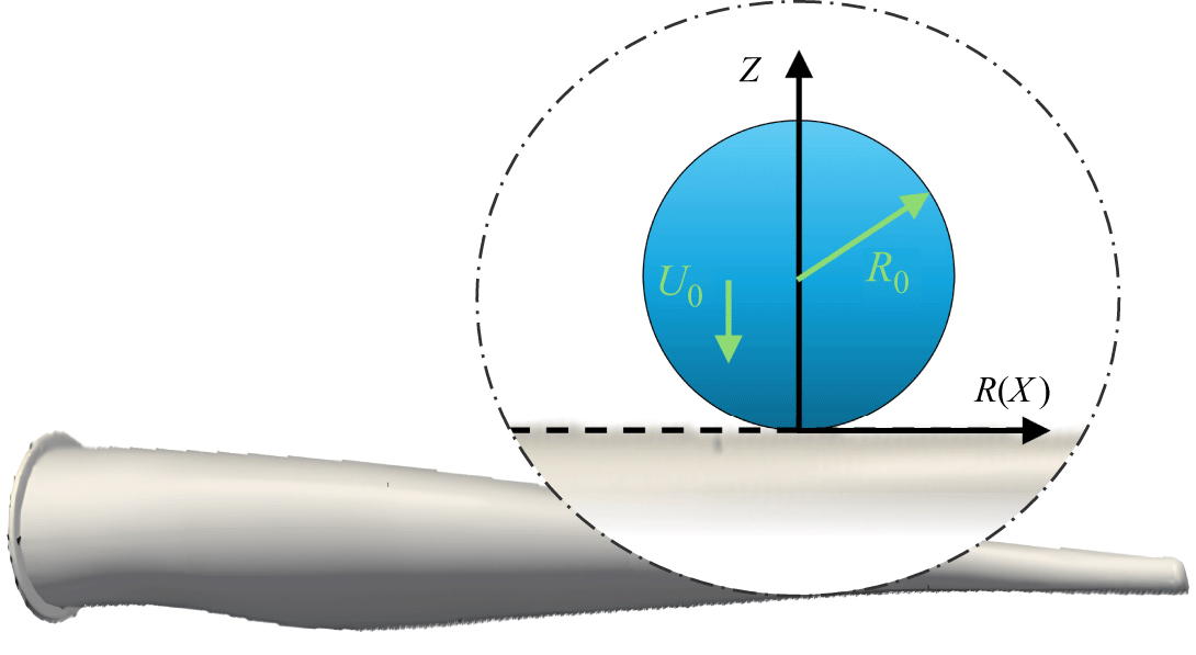
 R0
R0 U0
U0 r
r x
x z
z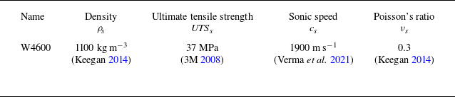
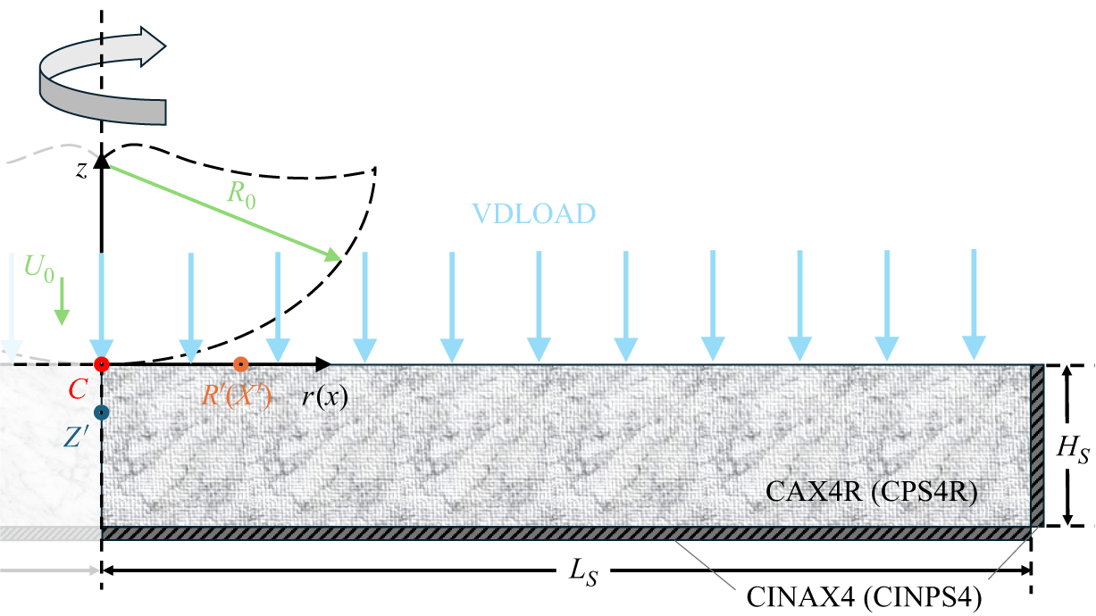
 z
z
 U0=50
U0=50 ms−1
ms−1 a
a μs
μs b
b μs
μs c
c μs
μs d
d μs
μs e
e μs
μs f
f μs
μs g
g μs
μs h
h μs
μs i
i μs
μs
 a
a U0=50
U0=50 ms−1
ms−1 b
b U0=90
U0=90 ms−1
ms−1 c
c U0=50
U0=50 ms−1
ms−1 ai
ai μs
μs bi
bi μs
μs ci
ci μs
μs aii
aii μs
μs bii
bii μs
μs cii
cii μs
μs aiii
aiii μs
μs biii
biii μs
μs ciii
ciii μs
μs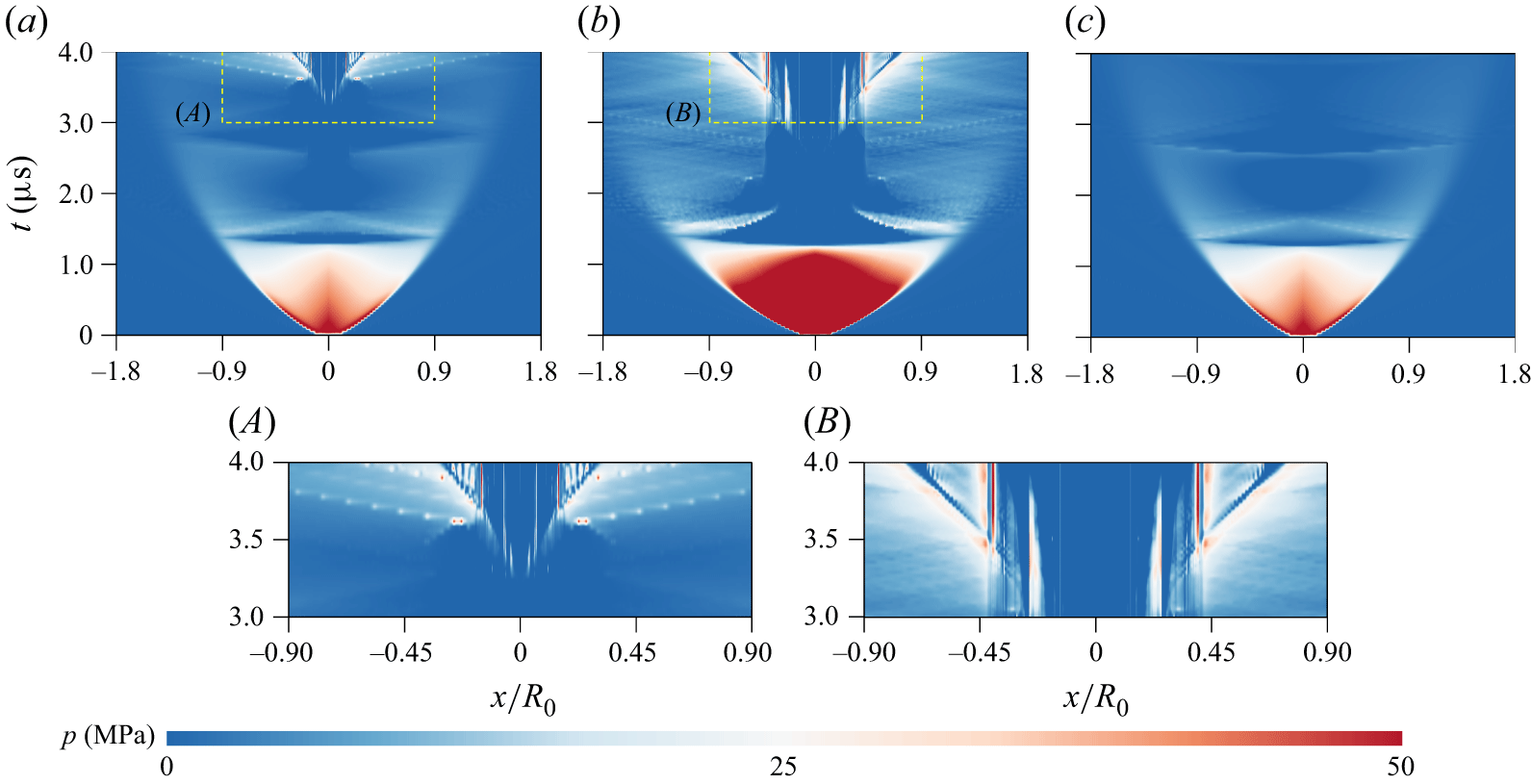
 a
a U0=50
U0=50 ms−1
ms−1 b
b U0=90
U0=90 ms−1
ms−1 c
c U0=50
U0=50 ms−1
ms−1 (A)
(A) (B)
(B) a
a b
b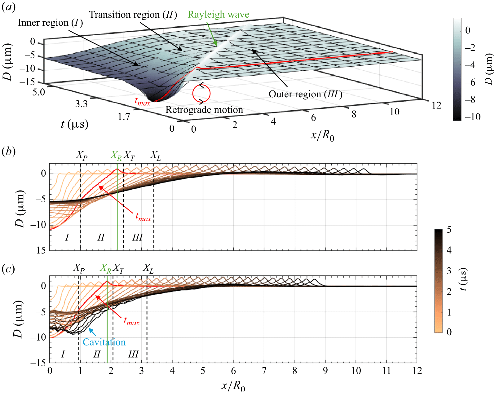
 U0=50
U0=50 ms−1
ms−1 0
0 5.2
5.2 μs
μs 0.16
0.16 μs
μs tmax≈1.1
 μs
μs 10.8
10.8 μm
μm 10.0
10.0 μm
μm tmax
tmax XP
XP XT
XT XL
XL I
I II
II III
III XR
XR
 U0=50
U0=50 ms−1
ms−1 t≈
t≈ 0.59
0.59 μs
μs 0.80
0.80 μs
μs 1.28
1.28 μs
μs 1.56
1.56 μs
μs 1.94
1.94 μs
μs 2.78
2.78 μs
μs 3.78
3.78 μs
μs 4.09
4.09 μs
μs 4.40
4.40 μs
μs 5.00
5.00 μs
μs XP
XP
 U0=50
U0=50 ms−1
ms−1 XP
XP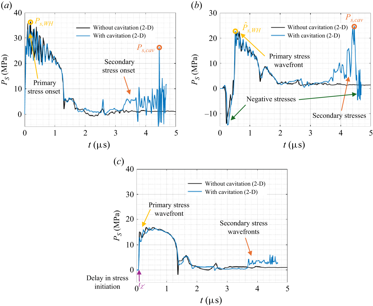
 y
y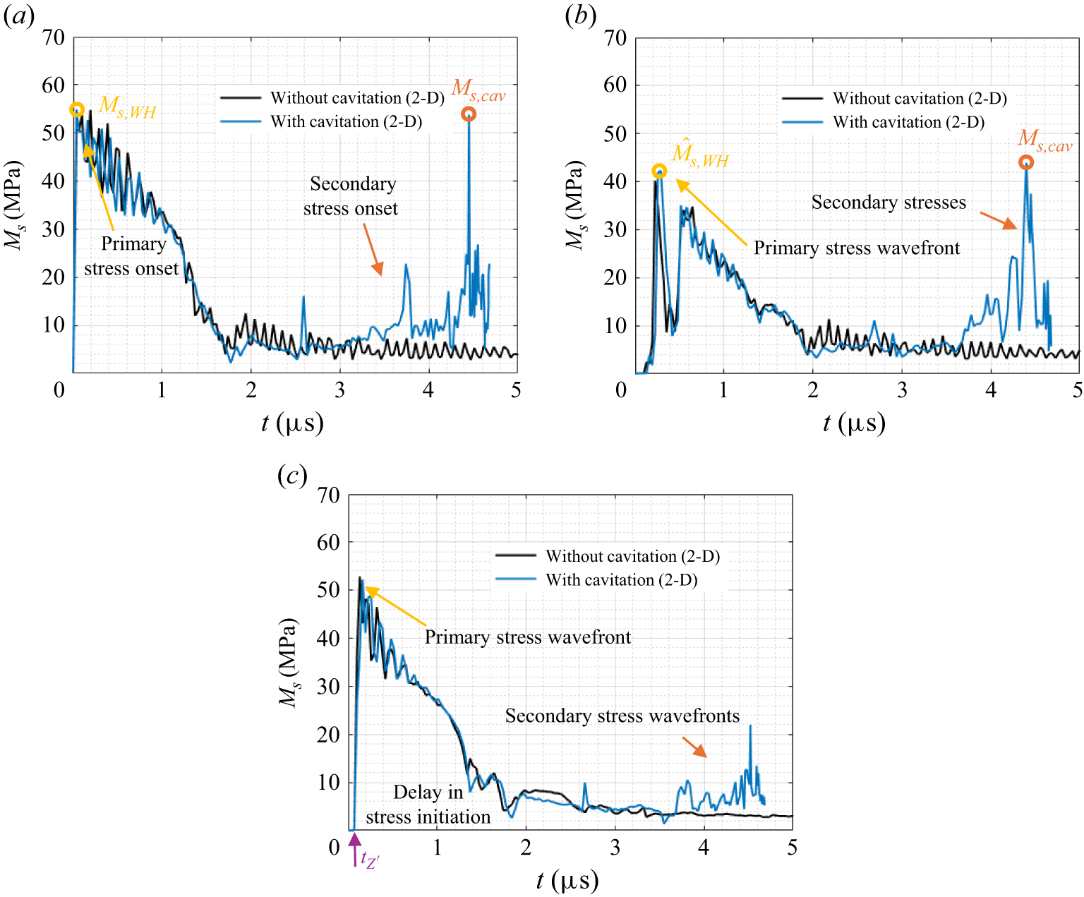
 y
y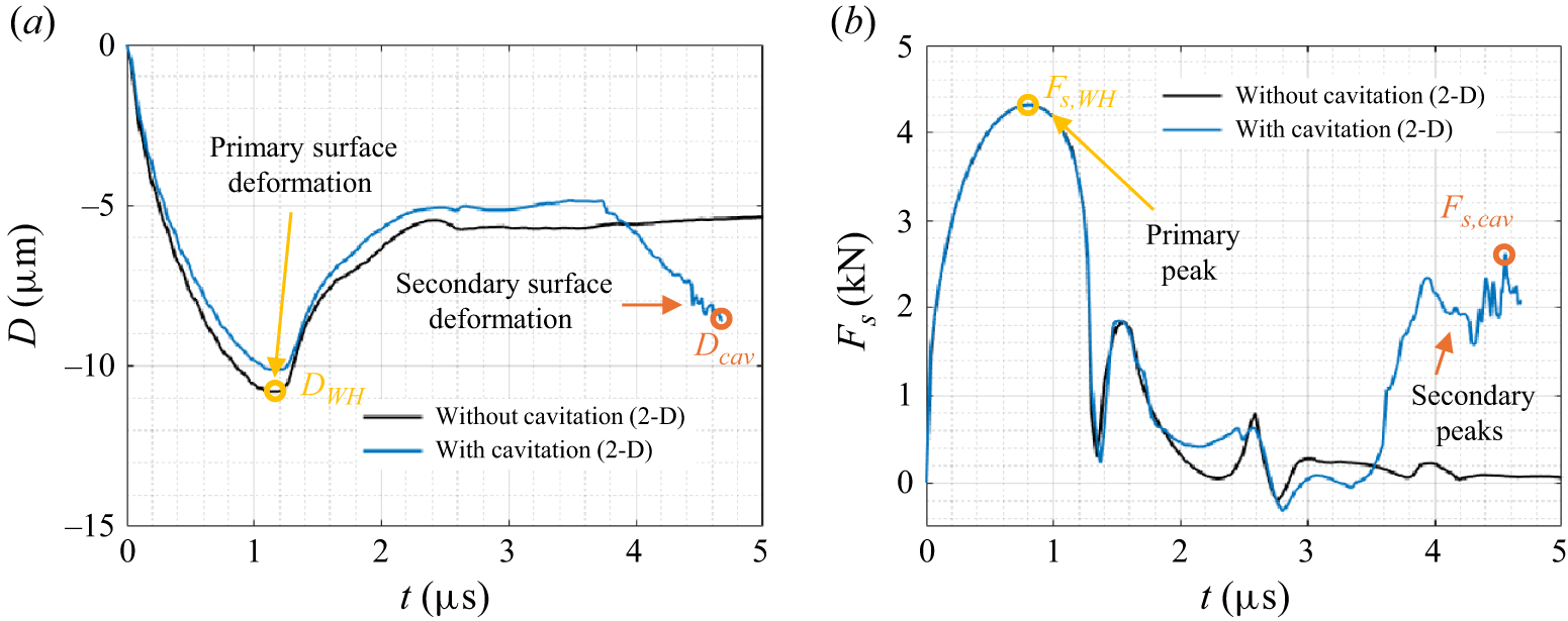

 a
a U0=50
U0=50 ms−1
ms−1 b
b U0=50
U0=50 ms−1
ms−1 c
c U0=70
U0=70 ms−1
ms−1 ai
ai μs
μs bi
bi μs
μs ci
ci μs
μs aii
aii μs
μs bii
bii μs
μs cii
cii μs
μs aiii
aiii μs
μs biii
biii μs
μs ciii
ciii μs
μs aiv
aiv civ
civ aiii
aiii ciii
ciii (r,z)
(r,z) R0
R0
 U0=50
U0=50 ms−1
ms−1 tcs/R0=0.0
 1.2
1.2 2.4
2.4 3.6
3.6 4.8
4.8 L0/R0=1.06
 H0/R0=0.29
 ρlU0cs
 U0=50
U0=50 ms−1
ms−1 U0=50
U0=50 ms−1
ms−1 U0=70
U0=70 ms−1
ms−1 t≈
t≈ 0.79
0.79 μs
μs 1.31
1.31 μs
μs 2.02
2.02 μs
μs 2.44
2.44 μs
μs 2.86
2.86 μs
μs 3.09
3.09 μs
μs 3.47
3.47 μs
μs 3.93
3.93 μs
μs XP
XP τ/(ρlU02)=−0.6
 0.6
0.6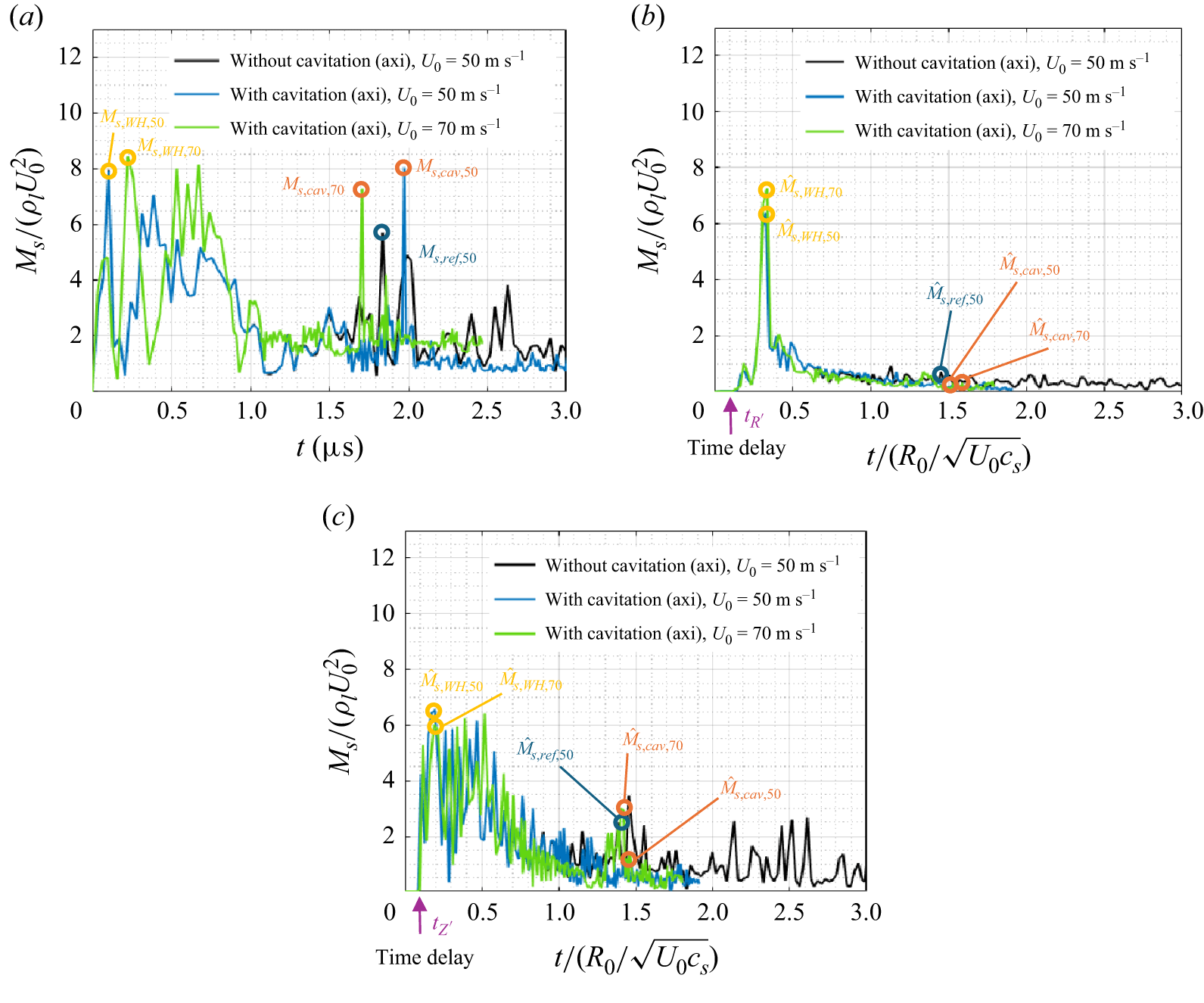
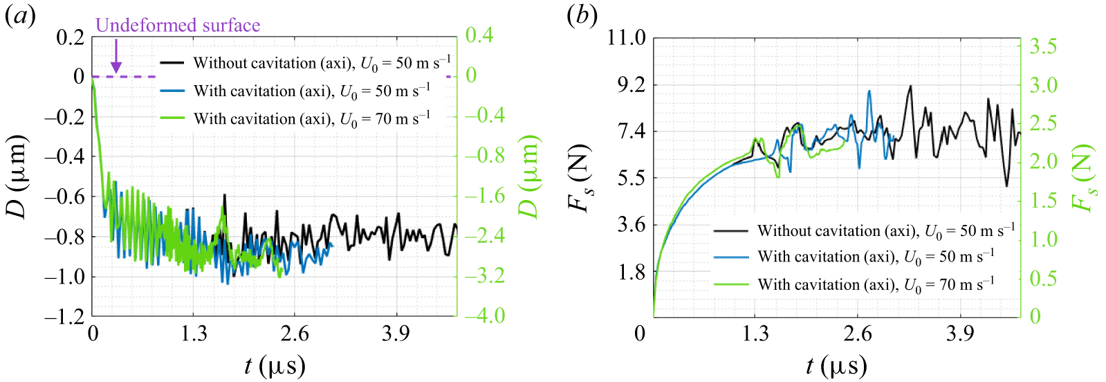
 U0=70
U0=70 ms−1
ms−1 D/(U02/Uref2)=−1.2
 0.2
0.2 Fs/(ρlU02R02)=3.0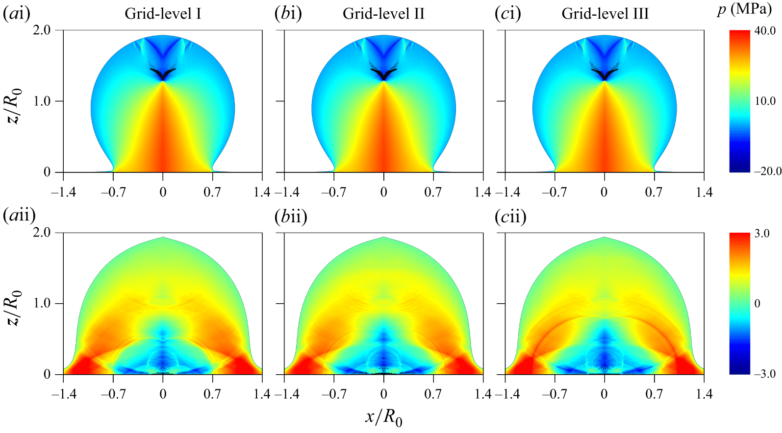
 t=0.8735
 μs
μs t=2.7286
 μs
μs U0=50
U0=50 ms−1
ms−1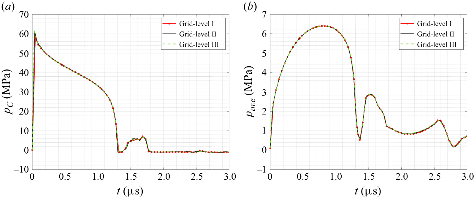
 a
a C(0.0,0.0)
 b
b U0=50
U0=50 ms−1
ms−1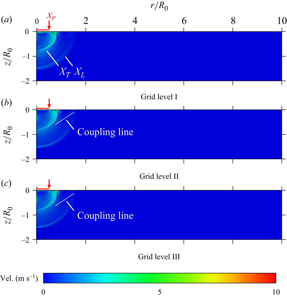
 t=0.98
 μs
μs U0=50
U0=50 ms−1
ms−1 XT
XT XL
XL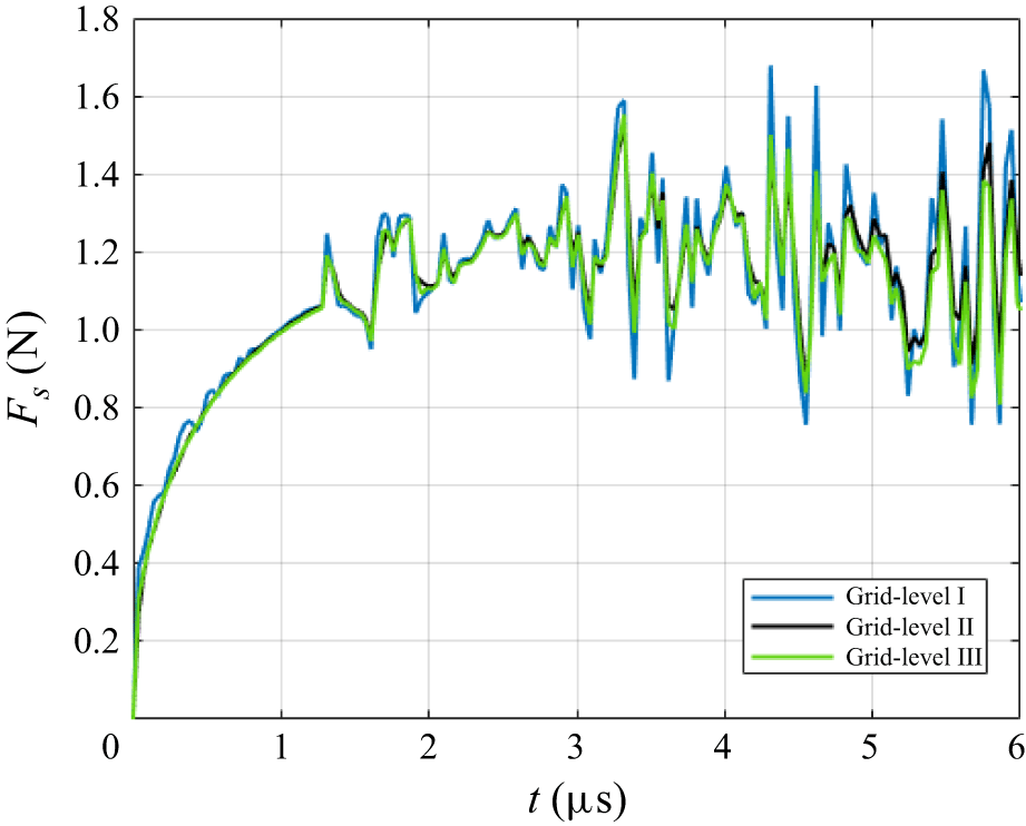
 U0=50
U0=50 ms−1
ms−1
 a
a phom=−10
 MPa
MPa b
b phom=−5
 MPa
MPa c
c phom=−1
 MPa
MPa ai
ai μs
μs bi
bi μs
μs ci
ci μs
μs aii
aii μs
μs bii
bii μs
μs cii
cii μs
μs aiii
aiii μs
μs biii
biii μs
μs ciii
ciii μs
μs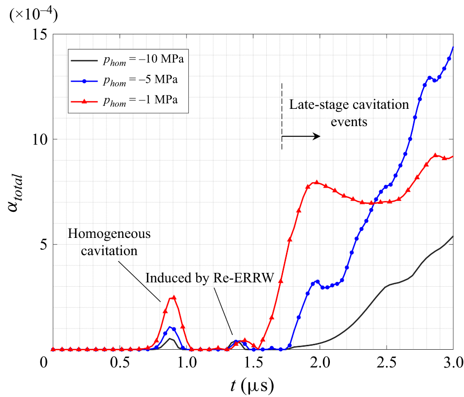
 phom=−10
 −5
−5 −1
−1 MPa
MPa
 Open access

