

INTRODUCTION
Sea ice is a major part of the Earth's cryosphere, and change in its area is an indicator of climate change and variability. Passive microwave sensors provide valuable data for sea-ice studies as they have broad spatial coverage and are able to retrieve data irrespective of time of day and most weather conditions. Appropriate analyses of these data provide estimates of sea ice concentration (IC). However, atmospheric conditions, such as precipitating clouds, and surface conditions such as melting can strongly influence the microwave signals measured by the sensors and thus the retrieved accuracy of the sea IC. Maps of sea IC are used to route ships, as well as input to numerical climate models of the atmosphere and ocean, and accurate representation of polynyas is also crucial to understanding ice and dense water production rates in the Antarctic. Therefore the accuracy of sea IC retrieval from satellite data is of prime importance.
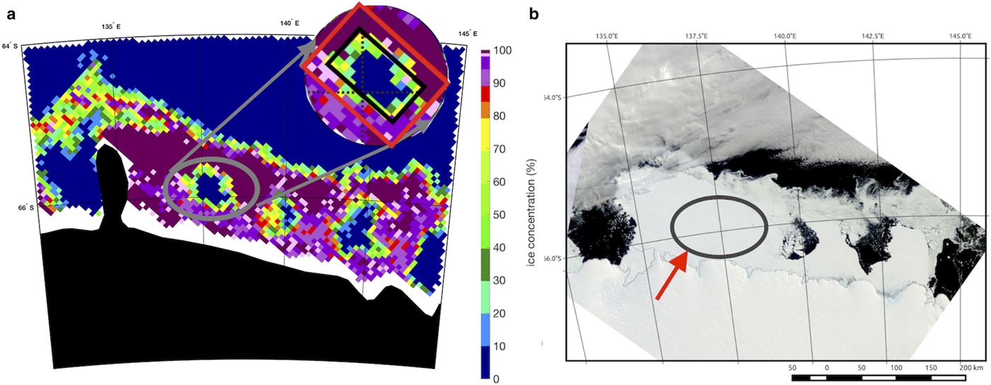
Discrepancies have been observed between IC maps produced by the ARTIST (Arctic Radiation and Turbulence Interaction STudy) Sea Ice (ASI) algorithm (Kaleschke and others, Reference Kaleschke2001; Spreen and others, Reference Spreen, Kaleschke and Heygster2008) and MODIS (Moderate Resolution Imaging Spectrometer) corrected reflectance True Colour images (Hall and others, Reference Hall, Salomonson and Riggs2006) near the Dibble Glacier in East Antarctica in February 2014. At 137.5°E 65.7°S, ASI daily IC maps show a cluster of pixels of 0% IC (Fig. 1), whereas MODIS images show full coverage by landfast sea ice. Subsequently, the artefact was also observed in other IC datasets.
(a) The studied artefact (in grey circle) on 20 February 2014 as identified in the ASI IC map. Magnified circle illustrates the inner box (within the black frame) and the outer frame (between the black and the red frame) used to identify the artefact. (b) MODIS True Colour image from that day. The red arrows indicate the artefact location as observed in (a). Note that the black area in the IC map in (a) depicts the land mask that has been applied, and which no longer matches the current shelf outline as can be seen in (b).
These discrepancies indicate localised misinterpretation of brightness temperatures (T Bs) by the ASI algorithm (and other algorithms, as we shall see later). The polynya-like artefact occurred in ASI maps from 2 February to 18 April 2014, with the exception of 12–18 February when the area shows full ice cover in ASI maps. The artefact also occurs in some, but not all, other sea IC datasets that are based on different retrieval algorithms and/or satellite data sources.
Here, we investigate (1) possible causes of the artefact, and (2) if the observed artefact is unique or if a similar anomaly has occurred at other times and other places. The motivation is as follows: (a) to better understand the physics of the interaction of radiation at microwave wavelengths with sea ice and snow; (b) to determine the frequency of occurrence of such artefacts, as they affect estimations on sea-ice area (the studied artefact had an average size of 5000 km2); and (c) to improve the ASI retrieval algorithm to eliminate such artefacts, as it limits the validity of passive microwave IC maps for shipping, offshore operations and sea-ice estimations and associated calculations.
DATA
Ice concentration
Many of the common IC retrieval algorithms determine IC based on parameters calculated from brightness temperatures (T Bs), such as polarisation ratio and gradient ratio (Comiso, Reference Comiso1995; Spreen and others, Reference Spreen, Kaleschke and Heygster2008; Comiso and Cho, Reference Comiso and Cho2013; Brucker and others, Reference Brucker, Cavalieri, Markus and Ivanoff2014; Tonboe and others, Reference Tonboe, Lavelle, Pfeiffer and Howe2016). Weather filters are applied to correct for the influence of atmospheric phenomena and effects, such as precipitation, cloud liquid water content and water vapour on the microwave brightness temperatures measured by radiometers on satellites. In this study, we focus on the time period from January to May 2014, during which the artefact is observed. IC maps based on different frequency-channel combinations and derived by the following algorithms on selected dates were investigated:
1. ASI algorithm based on AMSR-E and AMSR2 T Bs (Spreen and others, Reference Spreen, Kaleschke and Heygster2008), 89 GHz channels (horizontal, H and vertical, V, polarisation) for IC, lower frequencies as weather filter(s); data published by the Institute of Environmental Physics (IUP), University of Bremen (http://www.seaice.uni-bremen.de);
2. Bootstrap algorithm tuned by Japan Aerospace Exploration Agency (JAXA, global.jaxa.jp) (Comiso and Cho, Reference Comiso and Cho2013) based on AMSR2 T Bs, 19 and 37 GHz for IC, together with 23 GHz as weather filter, published by JAXA;
3. Bootstrap algorithm based on SSM/I and SSMIS T Bs (Comiso, Reference Comiso1995), 19 and 37 GHz plus weather filter, published by National Snow and Ice Data Center (NSIDC, nsidc.org);
4. NASA Team (NT) algorithm (Brucker and others, Reference Brucker, Cavalieri, Markus and Ivanoff2014) based on SSM/I and SSMIS T Bs, 19 and 37 GHz plus weather filter, published by NSIDC;
5. Ocean and Sea Ice Satellite Application Facility (OSI-SAF) sea IC algorithm (Tonboe and others, Reference Tonboe, Lavelle, Pfeiffer and Howe2016) based on SSM/I and SSMIS T Bs, 19 and 37 GHz plus weather filter, published by OSI-SAF (osi-saf.org).
Most of the above algorithms use weather filters to remove spurious values of non-zero IC on open water that result from atmospheric effects. In particular, the ASI and Bootstrap algorithms use the gradient ratio (GR) of the 36.5 and 18.7 GHz channels (hereinafter denoted as 37 and 19 GHz, respectively) to filter out cases where there is large cloud liquid water content:
 $$ {{\rm GR}(37/19) =} \displaystyle{{T_{\rm B}(37,V) - T_{\rm B}(19,V)} \over {T_{\rm B}(37,V) + T_{\rm B}(19,V)}} . $$
Moreover, the GR(24/19) is used to filter out high water vapour cases (using the 23.8 and 18.7 GHz channels, hereinafter denoted as 24 and 19 GHz, respectively).
Visual satellite data
In the Antarctic seasonal ice zone, in situ data are generally not available, and visual observations of the region are scarce. MODIS corrected reflectance True Colour images (Hall and others, Reference Hall, Salomonson and Riggs2006) were used to represent actual surface conditions. The images are available daily at 250 m resolution. Frequent cloud cover, however, hampers surface monitoring but, due to the wide swath width and high revisit frequency of the two MODIS instruments, several cloud-free cases could be identified.
Environmental parameters
The environmental conditions at the location during the study period are represented by 2-m air temperature and snowfall data from the European Centre for Medium-Range Weather Forecasts (ECMWF) Reanalysis (ERA)-Interim dataset (Dee and others, Reference Dee2011). Data corresponding to 1200 UTC with a grid spacing of 0.75° × 0.75° were used. In addition, the bathymetry of the studied area was examined using data from the bathymetry data compilation Bedmap2 (Fretwell and others, Reference Fretwell2013; Greene and others, Reference Greene, Gwyther and Blankenship2017), http://www.antarctica.ac.uk/bedmap2.
OBSERVATIONS ON ARTEFACT OCCURRENCE
We define the artefact to be an area where IC derived from satellite microwave T B data is notably less than that represented by the corresponding optical images. In some cases, the underestimation is such that where the optical images show ice coverage, the satellite-derived IC maps report 0%, thus showing a polynya-like feature.
Artefact occurrence in ASI data
In order to quantify the occurrence of the artefact at the same location, a rectangular area of 81.25 km × 175 km (13 × 28 pixels on the ASI 6.25 km grid), centred on 137.5°E 65.7°S, was outlined for further investigations. The selection is based on the ASI IC map on 9 February, 2014, which shows one of the largest extents of the artefact during the study period. A parameter, termed box-to-frame ratio, is defined to characterise the artefact as follows. Within the previously defined study area of 13 × 28 pixels, a concentric rectangular box of 9 × 20 pixels is outlined. This box is referred to as ‘inner box’, and the area in the larger (13 × 28 pixels) box that surrounds the ‘inner box’ is referred to as ‘outer frame’ (Fig. 1). Then, we define
 $$\hbox{Box-to-frame ratio}= {{\hbox{Average IC in the inner box}} \over {\hbox{Average IC in the outer frame}}}.$$
When the average IC in the outer frame is <40%, the result is discarded, as in such cases summer melt is presumed to dominate the study area. In principle, when the whole area is mostly covered by ice, the ratio will tend to unity. If the artefact appears, the ratio will be below 1. The variability of the ice edge and summer melt, when not discarded by the 40% threshold, can cause values above 1, which are not of interest here as they are not related to the artefact.
We use the period October 2002 to December 2015 to identify when and how often the artefact appears at the given location (Fig. 2). AMSR-E ceased operation in late 2011 and AMSR2 did not commence operation until the mid-2012, hence the missing data in 2012. There are also seasonal discontinuities when the occurrence of summer melt results in average IC in the outer frame to be less than the 40% threshold.
Time series of the ASI box-to-frame ratio from October 2002 to December 2015. Negative values, i.e. the grey-shaded area, indicate the periods of artefact occurrence. Summers with low sea-ice area were masked out with a 40% IC threshold. The gap in 2011/12 is caused by the unavailability of AMSR-E/2 data.
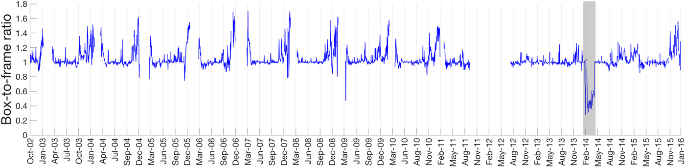
In Figure 2, only the drop of the ratio in early 2014 corresponds to an artefact occurrence. Similar artefacts did not occur at the study location on the ASI IC maps during the more than 10 years before 2014. Note, however, that similar artefacts have been found in five other locations between February and April, 2014 (see details in subsection ‘Identification of other artefacts’).
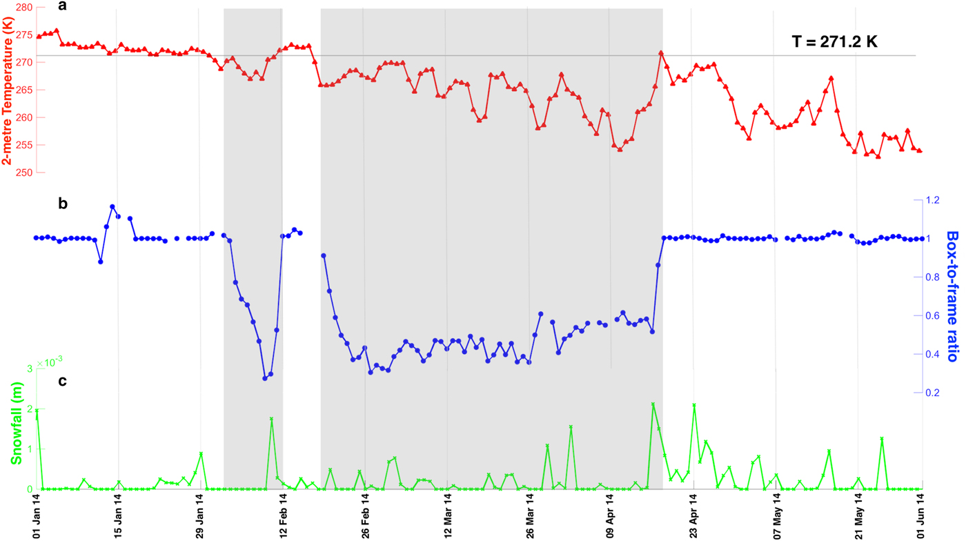
We have reviewed the location in ASI IC maps for 2014. The artefact occurred from 2 February to 18 April, 2014 in a region centred at 136°E 66°S. From 2 February, the artefact appeared and grew gradually in size; on 12 February it disappeared and the location had values near 100% on the IC maps until 18 February; from 19 February the artefact appeared again and remained until 17 April, during which time its size varied (Fig. 3). After 17 April, such an artefact was not observed again on the ASI IC maps at this location.
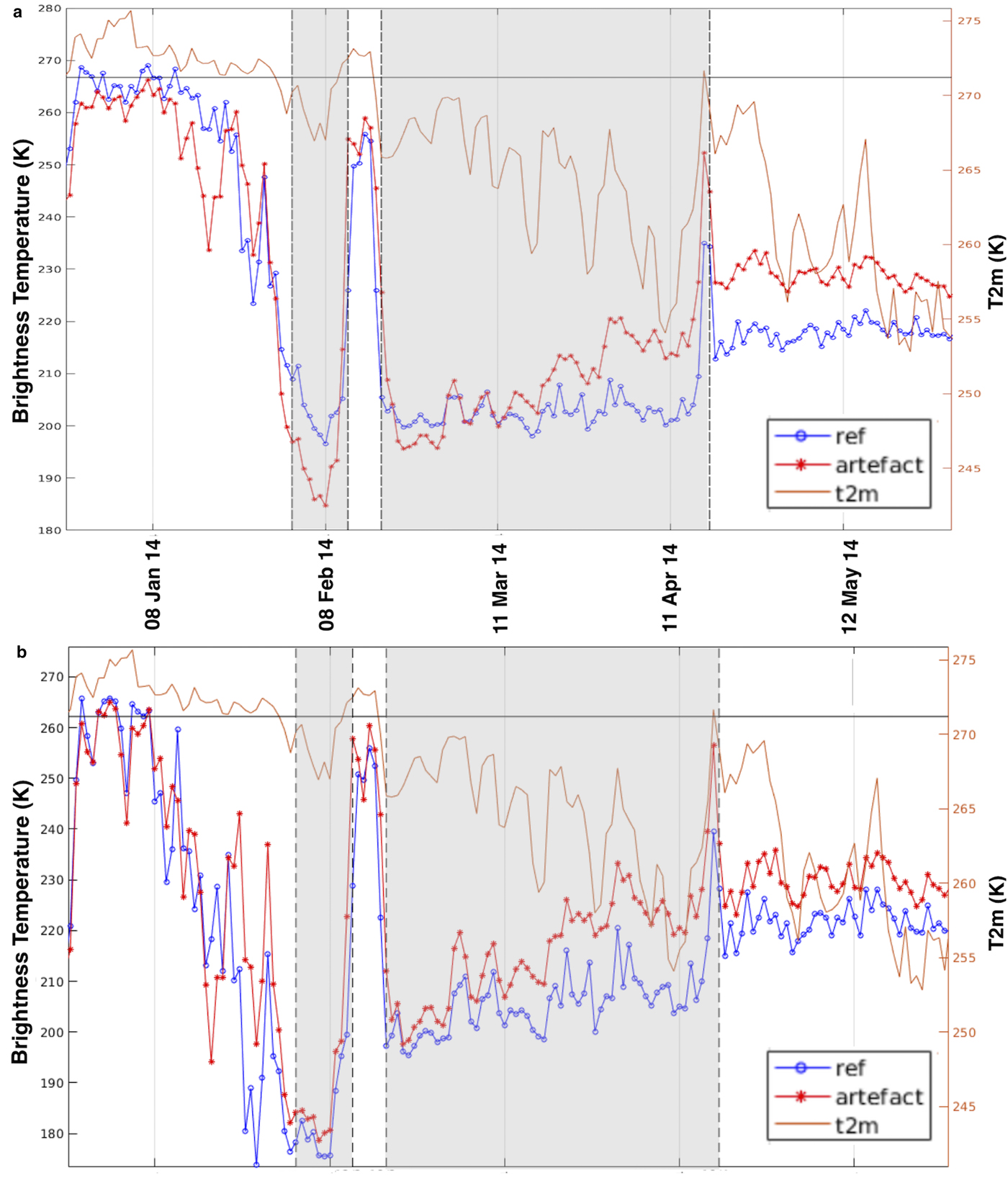
Time series of (a) 2-m temperature, (b) ASI box-to-frame ratio, and (c) snowfall (snow water equivalent), at the location of the artefact between January and May 2014. The horizontal black solid line indicates the temperature of 271.2 K on the top left axis. The grey shades indicate the periods of artefact occurrence.
In total, the artefact occurred during 68 days. Throughout this period, MODIS images show that the location is covered by ice (Fig. 4f), and do not show any polynya features (Fig. 4a).
IC maps on 20 February 2014 by various algorithms: (a) ASI AMSR2 (IUP); (b) Bootstrap AMSR2 (JAXA); (c) Bootstrap SSM/I (NSIDC); (d) NASA Team SSM/I (NSIDC); (e) OSI-SAF SSM/I; and (f) MODIS True Colour image of that day. Red arrows indicate the artefact location as observed in ASI maps.
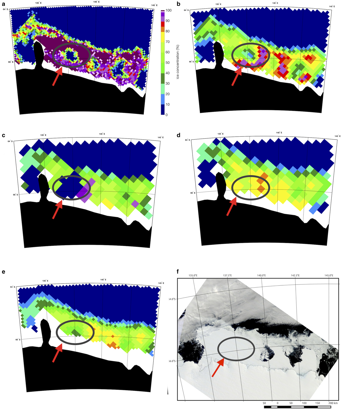
Artefact occurrence in other datasets
On 20 February 2014, the MODIS optical image shows cloud-free condition and reports no open water area at the artefact location (Fig. 4f). Real polynyas are observed on ASI maps at around 66°S and between 130°E and 135°E, at 140°E, and at 142.5°E (Fig. 4a), respectively, as confirmed by the MODIS image (Fig. 4f). The artefact appears in ASI IC maps at around 137.5°E 65.7°S. The same artefact also appears on Bootstrap maps based on AMSR2 (Fig. 4b) and SSM/I T Bs (Fig. 4c). AMSR2 Bootstrap maps do not show the smaller real polynya at 140°E, while SSM/I Bootstrap maps miss both real polynyas at 140°E and 142.5°E. In contrast, IC maps retrieved by the NASA Team algorithm (Fig. 4d) and OSI-SAF algorithm (Fig. 4e) based on SSM/I T Bs do not show an open water area at the study location. Instead, they show IC values between 40 and 60%. These values are similar to the IC shown for the real polynyas by these two algorithms. In addition, the ICs are also underestimated for fully ice-covered areas compared with ASI IC maps and MODIS imagery.
Weather filter effects
It was shown that the artefact is clearly present in the ASI and Bootstrap algorithm maps and some indication of it is seen with all algorithms. Therefore the radiometric response in at least some of the microwave channels used must show either a signature similar to that of open water or a detected weather influence so that IC is set to 0% by the weather filters in the algorithms. Here we investigate which channels make the main contribution.
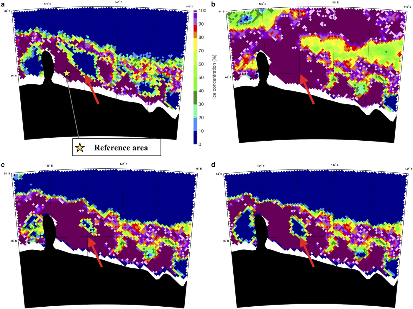
As seen before, the ASI and Bootstrap results show a similar response. Both use similar weather filters and the Bootstrap solution is used as an additional weather filter in the ASI algorithm. The Bootstrap, and the GR(37/19) and GR(24/19) weather filters were selectively turned off to study their impact on the ASI IC retrieval and their potential contributions to the occurrence of the artefact. Six weather filter configurations were investigated for the period from 1 February to 30 April, 2014, as summarised in Table 1. Figure 5 shows the resulting maps for four configurations for an example day on 9 February 2014.
ASI IC maps on 9 February 2014 with various configurations of weather filters: (a) Bootstrap filter and both weather filters on, (b) all filters off, (c) only GR(24/19) filter on and (d) only GR(37/19) filter on. Red arrows indicate the artefact location. The yellow star (along 66°S) in (a) marks the location of the reference area used for Figure 6.
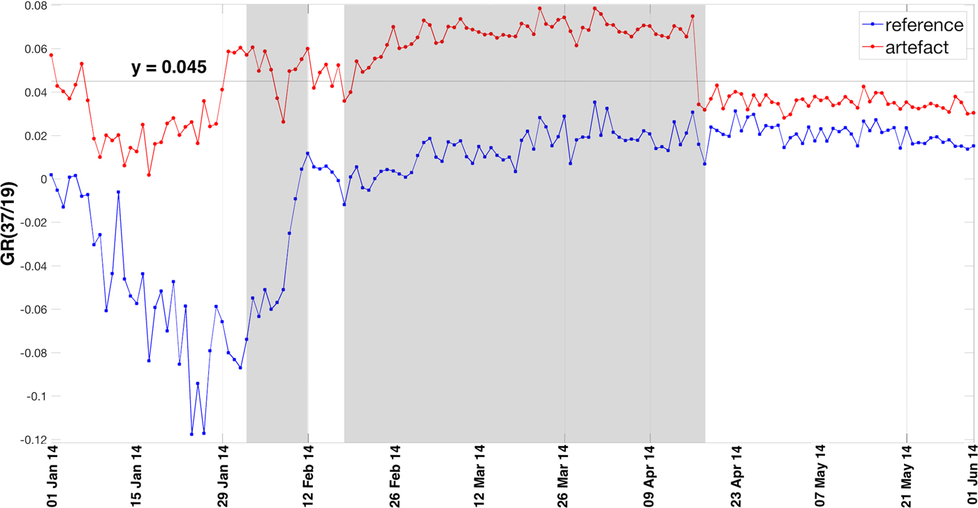
Time series of the maximum gradient ratio GR(37/19) of the pixels in the artefact (red curve) and in the reference area (blue curve) between January and May 2014. The horizontal black solid line indicates the threshold of 0.045 used by the GR(37/19) filter in the ASI algorithm. The grey shades indicate the periods of artefact occurrence.
The effect of the Bootstrap filter and the weather filters on the occurrence of the artefact
*Total number of days studied = 89 (1 February–30 April 2014).
First, if all filters are turned off (configuration 3 in Table 1 and Fig. 5b), the artefact does not appear, but lots of spurious ice is retrieved over open water. Thus the 89 GHz channels used in the ASI algorithm for the IC retrieval are not the cause of the artefact. When only one of the weather filters was turned on, the status of the Bootstrap filter (on or off) did not make any difference at the study location. Therefore only the configurations with one of the weather filters on and the Bootstrap filter off were investigated.
Of the two weather filters, the GR(37/19) has the strongest effect on the artefact (Case 5 in Table 1 and Fig. 5d) and is therefore studied in more detail. For comparison, a reference area near the artefact location was chosen. It is centred at 135.75°E, 66.67°S, where no artefact has been observed throughout the study period. This area is 390 km2 in ground spatial size (2 × 5 pixels on the ASI 6.25 km grid, Fig. 5a). GR(37/19) is calculated from daily averages of T Bs at 17 and 37 GHz at vertical polarisation. Figure 6 shows a time series of maximum GR(37/19) from the pixels in the artefact area and in the reference area. The value in the artefact area is generally higher than that in the reference area. In particular, maximum GR(37/19) in the artefact area exceeds the 0.045 threshold used for the ASI weather filter during artefact occurrence.
We look further into the time series of T Bs at 19 and 37 GHz at vertical polarisation (Fig. 7), which are the two channels used in calculating GR(37/19). For both channels, the difference between the average values in the artefact region and that in the reference area is significant when the artefact occurs, while the differences are small from 12 to 18 February. We note that after 18 April, the differences remain even though the artefact is not observed. This is because T Bs at both channels attain similar values in the artefact region, therefore the calculated GR(37/19) approaches zero and the weather filter is not triggered, thus the artefact is not produced. The differences after 18 April may hint at surface property changes following the artefact occurrence in the region when compared with the reference area.
Time series of the average brightness temperatures at (a) 18.7 and (b) 36.5 GHz in the vertical polarisation among the pixels in the artefact (red curve) and in the reference area (blue curve) between January and May 2014. The orange curve on the right axes shows the 2-m air temperature. The grey shades indicate the periods of artefact occurrence.
Location of the artefact
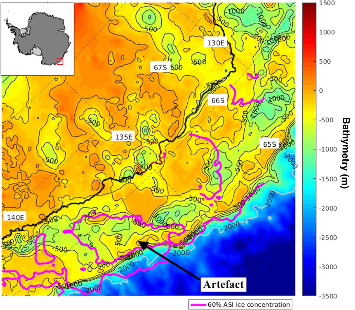
In order to find out why the artefact has appeared at the specific location, we plot the bathymetry map of the studied area. It indicates that the artefact is located above a trough running in the southwest–northeast direction, just north of 66°S, of maximum depth 1000 m, surrounded by sea bed of depth from 0 to 200 m (Fig. 8).
Bathymetry of the studied area. Black contour lines are at 250 m intervals from 0 to −1000 m. The thick black line represents the coast, i.e. the ice shelf boundary. Magenta lines represent the contour of ASI ice concentration of 60% on 9 February 2014, and black arrow indicates the position of the artefact on that day. Land data are calculated as ice surface elevation minus ice thickness.
Furthermore, we investigate some environmental parameters that could have contributed to conditions that produce the artefact. Figure 3 shows the time series of ERA-Interim 2-m air temperature (red curve, top) and snowfall (green curve, bottom) at the location of the artefact. Since one ERA-Interim grid cell (0.75° × 0.75°) is sufficient to cover the area of the artefact, the corresponding grid cell was identified and its 2-m air temperature and snowfall values were extracted and used for further analyses.
There is a drop from 272 K on 27 January 2014 to 268 K on 2 February, when the artefact first appeared. The temperature then fluctuates below the freezing point of sea water (~271.2 K) until 10 February. On 14 February it reaches 273 K. After 17 February there is a significant drop in the 2-m air temperature, and it remains fluctuating below freezing, reaching a minimum of 254 K on 10 April. From then on, the temperature steadily rises to 272 K on 17 April, after which it decreases and fluctuates again below freezing.
There are several notable snowfall events at the artefact location: on 29 January, 10 February and 16 April. Other snowfall events are also indicated in the ERA data throughout the study period. We note, however, that the quality of the ERA-Interim snowfall close to the coast may be limited, and the model grid is rather coarse (~80 km resolution). Therefore, the exact locations of local snowfall events remain unknown.
CORRECTION SCHEMES AND OTHER ARTEFACTS
The artefact appears in a region where there are real polynyas nearby, which can pose a danger for shipping, as one would expect to find a polynya based on the ASI and Bootstrap IC maps at the given location. In this section, we seek to correct the ASI algorithm and identify other potential artefacts.
Local correction scheme
Pixels of the artefact were replaced by those from a recalculated AMSR2 dataset using the ASI algorithm without Bootstrap and GR(37/19) filters. A box of 28 × 34 pixels within which the artefact occurred throughout the study period was defined. ICs in the box from the recalculated dataset were compared individually at each pixel to those from the original dataset. The higher value was kept at the corresponding pixel and the corrected maps were plotted. In this way, the artefact was eliminated using data that are not compromised by Bootstrap and GR(37/19) filters. The correction scheme was applied to all 89 original ASI data files from February to April 2014, and a corrected dataset was created.
The disadvantage of this scheme is that it only applies to this specific case of the artefact at the study location, and is applied after the event. In this correction scheme, the GR(24/19) filter was kept on to maintain weather filtering in the marginal ice zone. In the next section we provide a more general correction scheme.
General correction scheme
We propose to change the conditions for applying Bootstrap and GR(37/19) filters in the ASI algorithm. Originally these filters are applied to all data pixels. Since it is noted that they have caused the artefact, we want to prevent applying these filters to areas that are guaranteed to be ice-covered. We propose to apply these two filters only if the area was not fully ice covered the day before. As we will see, however, this can cause differences along the ice edge.
The two filters are only applied to pixels that (1) have GR(37/19) on the present day above the threshold of 0.045 and (2) have IC <30% on the previous day in the uncorrected dataset, in order to avoid erroneously setting ice-covered pixels to open water. This should eliminate possible artefacts in other locations that have causes similar to those of the studied artefact.
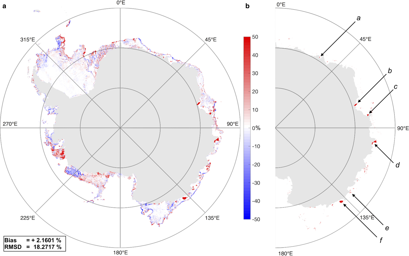
We have tested this correction scheme for ASI IC retrieval from 1 February to 30 April, 2014. The corrected IC maps do not show the artefact. However, there are significant disagreements between the corrected and the original IC along ice edges (Fig. 9a). Changing the threshold value of IC in the previous day does not improve the poor performance along ice edges. Better understanding of the occurrence of the artefact is required to devise a complete correction scheme.
(a) Deviation of the corrected ASI ICs from the original values on 3 March 2014. (b) Location of studied [f] and other artefacts [a–e] (see Fig. 10 and Table 2 for indexing). In (b) a binary colour scheme is used to highlight the locations and extent of artefacts, where red indicates those areas where deviations are >40%. Smaller values are displayed in white, i.e. are not plotted.
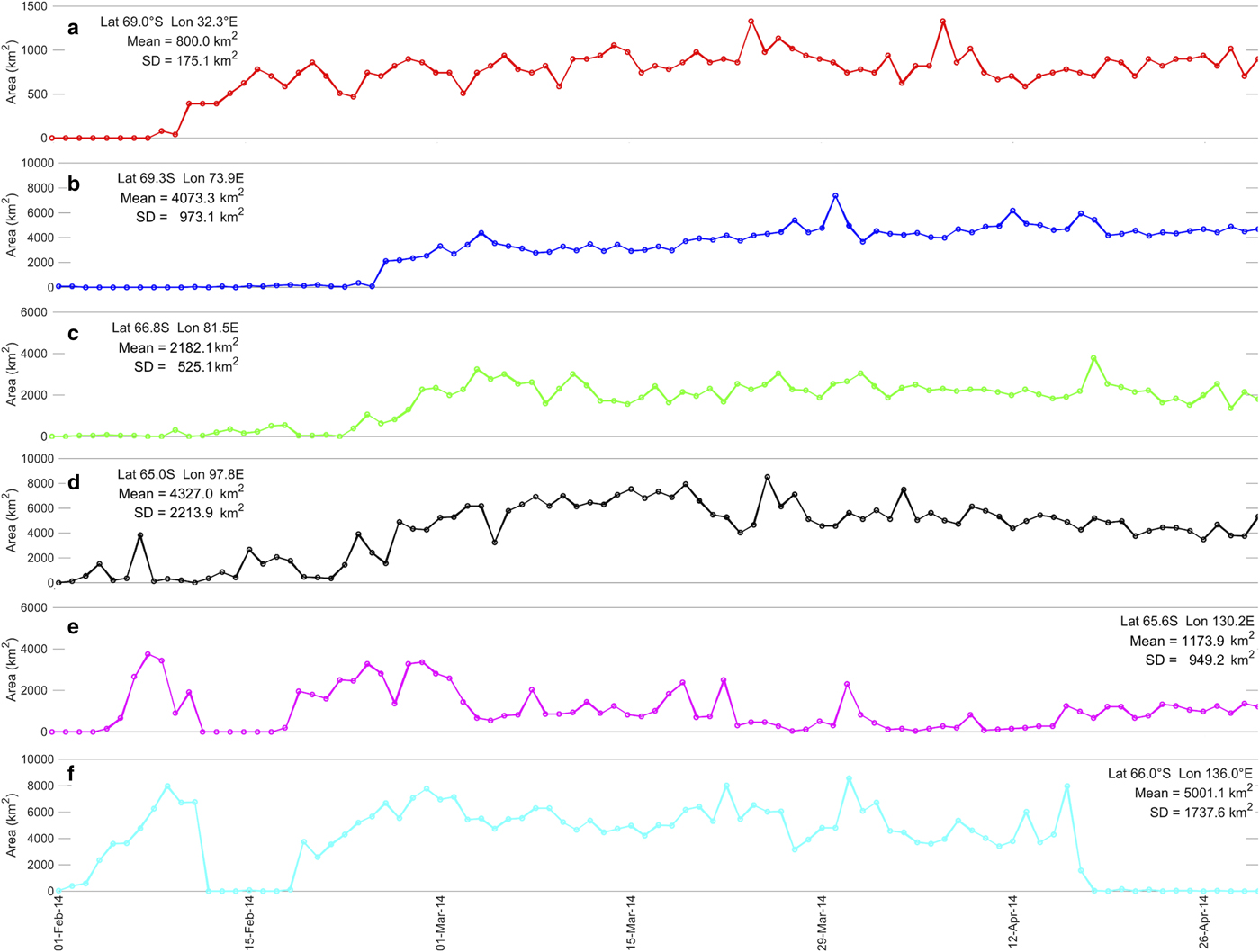
Time series of the area of the main artefact in this study (f) and other identified artefacts in January–April 2014. On each curve, the centre location of the artefact, its average area and standard deviation (SD) are displayed. Average areas are calculated by counting the number of data points where the deviation of the corrected ICs from the original ASI ICs is >40%, then multiplying it by the spatial area of a pixel (6.25 km × 6.25 km, i.e. 39 km2).
Occurrence of other artefacts from 1 February to 30 April 2014. See Figure 9 for a map of the documented cases.
*Average areas of artefacts are calculated by counting the number of data points where the deviation of the corrected ICs from the original ASI ICs is >40%, within the vicinity of their locations, then multiplying the spatial area of a pixel (6.25 km × 6.25 km). Averages and SD are taken throughout the period of 1 February to 30 April 2014.
Identification of other artefacts
Although the general correction scheme has the problems just described, it can be used as a semi-automatic method to identify potential artefacts at other locations. First, the deviation of the corrected ICs from the original ASI ICs is calculated (Fig. 9a). In the case of the studied artefact, the deviation is above +40%, and the deviation occurs at a consistent location. Figure 9a shows that there are vast areas where the deviation is above +40% (shown as red). Many of these, however, can be attributed to transient atmospheric effects and they disappear from one day to another. Based on these characteristics, we record and study other locations with a deviation above +40% IC after correction that last for at least 4 days, during the period 1 February to 30 April, 2014. We then compare the ASI maps to the corresponding MODIS images to verify that these cases were indeed artefacts, i.e. ice covered areas and not polynyas. This leads to the identification of five more artefacts. Figure 9b shows that these artefacts are either located in bay areas (for a and b) or at or near peninsulas. They are mostly located close to the coast or ice shelf boundary, i.e. they likely occur on fast ice. Figure 10 shows the change in area of our studied artefact and these five additional artefacts during the study period.
Since the used True Colour MODIS images begin to have less coverage on the Antarctic coast due to lack of visible light in winter from May onwards, the cross-referencing between ASI data and MODIS images continues only until the end of April. Another limitation is that MODIS images may show cloud cover over the location of potential artefact, obscuring the surface features and thus hindering the verification of IC maps.
DISCUSSION
Potential cause of the artefact
The appearance of the artefact on the ASI IC maps is due to the effect of Bootstrap and weather filters in the ASI algorithm. Turning on Bootstrap filter and GR(37/19) weather filter individually accounts for most of the appearance of the artefact. The GR(24/19) weather filter has a relatively small effect, accounting for only three occurrences (9 February, 2 and 3 March) of the artefact, with considerably smaller sizes than when all filters are turned on (Table 1). Turning off all the filters would eliminate the artefact completely, but would result in extensive appearance of spurious ice over open ocean (Fig. 5b), indicating the importance of the weather filters in IC retrieval at 89 GHz. The results suggest that both Bootstrap filter and GR(37/19) weather filter have misidentified the pixels at the location of the artefact as open water area, which led to the appearance of a surface feature that resembles a polynya, while in fact the area was ice covered, as evident in MODIS images.
We hypothesise that the artefact occurrence is related to environmental changes in the area at the time. From 11 to 17 February, the rise in temperature above freezing coincides with the first disappearance of the artefact. The two larger snowfall events (10 February and 16 April) coincide with rising air temperature and precede artefact disappearances (Fig. 3).
Variations of temperature and other snow properties can both alter the microwave signature of the ice surface. Temperature at the location fluctuated near the freezing point, suggesting that melt–refreeze processes of snow may be involved in generating the artefact. The snowfall events would lead to an accumulation of snow cover on the sea ice, which could metamorphose based on environmental conditions (e.g., air temperature, wind pattern), and thus modify the emissivity of the surface.
Snow wetting and refreezing are common and frequent on Antarctic sea ice in the Southern Ocean (Markus and Cavalieri, Reference Markus and Cavalieri2006). Refreezing leads to an increase in grain sizes (Colbeck, Reference Colbeck1982), enhances scattering within the frozen top layer of the snow, and reduces emissivity at 37 GHz relative to 19 GHz (Onstott and others, Reference Onstott, Grenfell, Matzler, Luther and Svendsen1987; Mätzler, Reference Mätzler1994). This would lower the GR(37/19). On the other hand, upon the melting or wetting of snow, emissivities at 19 and 37 GHz approach unity, thus GR(37/19) approaches zero, before becoming positive (Markus and Cavalieri, Reference Markus and Cavalieri2006). GR(37/19) is positive for water but near zero or negative for ice. If the snow cover on the sea ice is wetted either by flooding and/or melting, GR(37/19) will increase. If the value exceeds the threshold, GR(37/19) filter will be triggered and the pixel will be reported as ice-free by the ASI algorithm, even though it is actually snow-covered sea ice.
Moreover, for high snow loads, flooding can also occur at the snow/ice interface. Such flooding would cause the formation of slush, which can refreeze again if the temperature drops, and snow ice forms. The refreezing, however, will take time as the slush is more saline. These transformations would not affect the optical appearance of the snow layer, so that the flooded area would appear in MODIS images as snow/ice covered. Figure 6 supports these speculations. The 2-m air temperature in January is ~0 °C (Fig. 3) and melting or snow metamorphism can have occurred. GR(37/19) is above zero during that period but does not exceed the 0.045 threshold. Interestingly only after the temperature drops again to below the sea water freezing temperature on 2 February does the GR(37/19) increase above the threshold, which highlights the importance of the refreezing process for this phenomenon. In the reference area without artefact, from mid-February to mid-April 2014, the maximum GR(37/19) is below the threshold of 0.045, while the maximum in the artefact region is above the threshold. Thus the increase in GR(37/19), possibly caused by wetted and refrozen snow, is one of the reasons that the artefact is observed during the period.
We should note that the air temperature data used in these analyses do not necessarily represent the temperature at the sea ice surface, particularly when the near-surface air is not well mixed. It is possible for snow to melt or metamorphose at sub-zero air temperature, when snow crystals change shape due to the absorption of solar radiation (Colbeck, Reference Colbeck1989; Launiainen and Cheng, Reference Launiainen and Cheng1998). Also, fresh snow has low thermal conductivity due to its high air content. It can act as an insulator to trap heat and warm up the subsurface snow/ice layers (Pomeroy and Brun, Reference Pomeroy, Brun, Jones, Pomeroy, Walker and Hoham2001). At freezing temperatures, subsurface snow melting is sufficient to foster extensive snow metamorphism, and to form a surface ice layer when the wetted snow refreezes (Haas and others, Reference Haas, Thomas and Bareiss2001). All of these processes can affect the microwave signature of the ice surface.
The question remains why the artefact is so localised and is much smaller than the synoptic scale of the warming events. While we notice a correlation between the location of the artefact and the bathymetry in its vicinity, without additional data a conclusion cannot be drawn. We hypothesise that the regional ocean current and heat flux could play a role, but further investigations and modelling in the area are required. Different ocean heat fluxes steered by bathymetry could cause variability in sea ice thickness with the accompanied potential for ice flooding and slush as discussed above. Another possible explanation for the strong localisation could be related to katabatic winds along the coast associated with colder and dryer air. These winds can cause variability in surface temperature and thereby influence the melt–refreeze pattern and also can cause strong snow sublimation, which would influence the snow depth. According to Grazioli and others (Reference Grazioli2017), our artefact lies in a high snow sublimation area. Katabatic winds could also redistribute snow and thereby cause local flooding. We, however, have no data to support these hypotheses.
Performance of other retrieval algorithms
The artefact appears on IC maps retrieved by the Bootstrap algorithm both at JAXA – using AMSR2 T Bs – and at NSIDC – using SSM/I T Bs. This shows that the artefact is not limited to the AMSR2 ASI dataset (Fig. 4). There is no real artefact, but an area of reduced IC on the maps retrieved by NT algorithm or OSI-SAF algorithm, both using SSM/I T Bs. The NT algorithm uses the GR and the polarisation ratio of the 19 and 37 GHz T B to better estimate low ICs; while OSI-SAF algorithm calculates a weighted value using both Bootstrap and Bristol algorithms for IC below 40%. These frequency and channel combinations do not seem to cause a drop of IC to 0% and they both seem to use different weather filter thresholds that do not cause the artefact to appear.
We notice two more issues in the inter-algorithm comparison. First, ICs retrieved by Bootstrap, NT algorithm and OSI-SAF algorithms show general underestimation by 40–60% at the artefact location and its larger surrounding when compared with ASI IC maps and MODIS optical images, both of which show close to 100% concentration for most of the ice-covered area. Second, the 25 km-resolution of SSM/I Bootstrap, NT and OSI-SAF algorithm is not sufficient to resolve polynyas close to the artefact location (along 140°E and 142.5°E); these polynyas are present in ASI maps and MODIS optical images (Fig. 4a and f). Thus these algorithms do not show the artefact but on the other hand show a significant overestimation of IC for real polynyas.
Identification of other artefacts
We have identified five more similar artefacts during the study period in 2014 throughout the East Antarctic, suggesting that there are unexpected mechanisms causing the ASI algorithm to fail under specific circumstances. Incidentally, these artefacts are found to be located either in bay areas or near peninsulas and mainly on landfast ice. This indicates that regional weather conditions, land features and bathymetry, possibly contribute to producing the artefacts. Further investigations should be made to look for any correlations between the locations of the artefacts and their causes.
CONCLUSIONS
Erroneous ICs retrieved by several passive microwave retrieval algorithms have been identified at the study location, near the Dibble Glacier, Antarctica. From February to April 2014, MODIS optical images show complete ice cover at the location, where ASI and Bootstrap IC maps report an artefact that resembles a polynya. Such an artefact occurred in the ASI IC maps only in 2014 (Fig. 2). Bootstrap IC maps using AMSR-2 and SSM/I T Bs also showed the artefact from February to April 2014. SSM/I-based IC maps from NT algorithm and OSI-SAF algorithm did not show the artefact, but reduced IC at the same position. It should be noted that results from SSM/I Bootstrap, NTA, and OSI-SAF algorithms show underestimations in IC with respect to that from the ASI algorithm and MODIS images in a larger area around the artefact (Fig. 4).
The Bootstrap filter and the GR(37/19) weather filter in the ASI algorithm are the cause of the artefact in the ASI maps (Table 1). During the study period, GR(37/19) at the artefact location exceeded its threshold value, which leads to some pixels being set to 0% IC. Bootstrap IC was consistently low at the artefact location, presumably also related to GR(37/19), which also leads to pixels being set to 0%.
The occurrences of the artefact coincide with temperature fluctuations at the location. We speculate that melt–refreeze processes and snow metamorphism have led to the pixels being misinterpreted by the ASI and Bootstrap algorithms as open water. The reason for the artefact occurring at the specific location are unclear. The artefact, however, is located over a bathymetric trough (Fig. 8) and the artefact extent looks as if bathymetric steering of ocean currents could play a role. Other explanations, however, like influence of katabatic winds cannot be excluded as we do not have in-situ observations.
Location-specific and general correction schemes have been implemented to rectify the artefact in ASI IC maps. The location-specific correction ensures that the output ASI data agrees with the MODIS images. The general correction scheme, while correcting for the artefact, tends to introduce erroneous ICs along the ice margins (Fig. 9). However, it led to the discovery of five more similar artefacts from February to April 2014. Together they amount to an area of ~18 000 km2 that is misinterpreted as ice-free, which is ~0.5% of the February Antarctic sea ice area.
Taking into account the error rates of IC retrieval algorithms, the artefacts are of small statistical importance in climatological time series. However, the persistence of the event over more than 2 months excludes purely statistical effects such as sensor noise. While focusing only on one particular case, this study does have hemisphere-wide importance as such artefacts seem to be frequent. They will cause a bias in sea IC time series, for assessment of the contribution of polynyas to sea ice and dense water production, and are of importance for shipping. A holistic study into the subject might result in some improvement on the current sea IC retrieval methods.
ACKNOWLEDGMENTS
This project is financially supported by the ESA Climate Change Initiative, project on Sea Ice (SICCI-2) and by the Deutsche Forschungsgemeinschaft (DFG) in the framework of the priority programme ‘Antarctic research with comparative investigations in Arctic ice areas’ through grant SITAnt (SP 1128/2-1). AMSR-E and AMSR2 brightness temperatures were provided by the Earth Observation Research Centre, Japan Aerospace Exploration Agency (JAXA). ERA Interim data were provided by the European Centre for Medium-Range Weather Forecasts (ECMWF). AMSR-E Level 2A data were provided by NASA National Snow and Ice Data Center (NSIDC). Moderate Resolution Imaging Spectrometer (MODIS) corrected reflectance True Color images are available from the Worldview web application. We acknowledge the use of imagery provided by services from the Global Imagery Browse Services (GIBS), operated by the NASA/GSFC/Earth Science Data and Information System (ESDIS, https://earthdata.nasa.gov) with funding provided by NASA/HQ. We thank the two reviewers for very helpful comments that significantly improved the paper. We thank Larysa Istomina for discussions about the influence of katabatic winds on snow. Finally, we would like to acknowledge Patrice Godon of IPEV (Institut Polaire Français Paul Emile Victor), France, whose enquiry whether there was a polynya there brought the artefact to our attention.


 Open access