3.1. Undisturbed turbulent boundary layer

The wall-normal profile of the temporally and spatially averaged, normalized streamwise velocity $\langle \bar {U}_{1}\rangle ^{+}$ is depicted in figure 4 together with the ‘theoretical’ velocity profiles in the viscous sublayer, $U_1^+ = x_2^+$, and in the log layer, $U_1^+ = ({1}/{\kappa })\ln x_2^+ + B$ (‘log-law’; Pope Reference Pope2000), where $\kappa$ ($= 0.41$) denotes the von Kármán constant, and the intercept is $B = 5.0$. The spatial average was taken over the transverse and streamwise directions. In addition to the present data, laser Doppler velocimetry (LDV) measurements by De Graaff & Eaton (Reference De Graaff and Eaton2000) are also plotted in figure 4. As can be seen, for $x_2^+ \geq 8$, the wall-normal profile of $\langle \bar {U}_1\rangle ^+$ matches closely the measurements by De Graaff & Eaton (Reference De Graaff and Eaton2000) and log-law behaviour is observed for $30 \leq x_2^+ \leq 200$. Measurements by De Graaff & Eaton (Reference De Graaff and Eaton2000) were performed at higher momentum thickness Reynolds numbers $Re_\theta$, and as a result, the outer layer is shifted to larger $x_2^+$ values. Close to the wall ($x_2^+ < 8$), the tomo-PIV measurements deviate from the velocity profile in the viscous sublayer due to the finite size of the interrogation volume (van Hout et al. Reference van Hout, Eisma, Elsinga and Westerweel2018) and the strong gradients near the wall.

Figure 4.

Semi-logarithmic plot of $\langle \bar {U}_{1}\rangle ^{+}$ as a function of $x_{2}^{+}$. Present data: red squares denote ${Re_{\theta }}=850$; the dash-dot curve denotes the velocity profile in the viscous sublayer; the dashed line denotes the ‘log-law’. Literature results (De Graaff & Eaton Reference De Graaff and Eaton2000): diamonds denote ${Re_{\theta }}=1430$; triangles denote ${Re_{\theta }}=5200$.

The mean streamwise velocity at the edge of the boundary layer was estimated based on the plateau values that were reached farthest away from the wall, i.e. $U_{e}=0.189\pm 0.001\,{\rm m}\,{\rm s}^{-1}$ ($U_e/U_b = 1.086$). The boundary layer thickness $\delta = 43\pm 3$ mm was determined as the wall-normal position for which $\langle \bar {U}_1\rangle = 0.99U_e$. Based on the measured velocity profile, the displacement and momentum thicknesses were $\delta ^{*}=6.03\pm 0.03$ mm and $\theta =4.47\pm 0.05$ mm, respectively, giving a shape factor $H= \delta ^*/\theta = 1.35\pm 0.01$, i.e. within the range of typical values for TBLs (Schlichting & Gersten Reference Schlichting and Gersten2000). The momentum thickness Reynolds number was $Re_\theta =U_e\theta /\nu =850\pm 10$. The friction velocity $u_{\tau }=0.009\pm 0.001\,{\rm m}\,{\rm s}^{-1}$ was determined by the Clauser method (Clauser Reference Clauser1956) assuming $\kappa = 0.41$ and $B = 5.0$, giving friction Reynolds number $Re_\tau =u_\tau \delta /\nu =390\pm 50$.

Wall normal profiles of the normalized and spatially averaged Reynolds stress components, $\langle \overline {u_{1}u_{1}}\rangle ^+$, $\langle \overline {u_{2}u_{2}}\rangle ^+$ and $-\langle \overline {u_{1}u_{2}}\rangle ^+$, are depicted in figure 5 and also compared to measurements by De Graaff & Eaton (Reference De Graaff and Eaton2000) as well as hot-wire measurements by Erm & Joubert (Reference Erm and Joubert1991) ($Re_{\theta } = 697$ and 1003). The present results compare well with those of Erm & Joubert (Reference Erm and Joubert1991) and De Graaff & Eaton (Reference De Graaff and Eaton2000). However, note that in the tomo-PIV measurements, the $\langle \overline {u_1u_1}\rangle ^+$ profile becomes governed by noise for $x_2^+\leq 15$ (figure 5(a); see also van Hout et al. Reference van Hout, Eisma, Elsinga and Westerweel2018).

Figure 5.

Semi-logarithmic plots of the wall-normal profiles of the normalized Reynolds stress components: (a) $\langle \overline {u_1u_1}\rangle ^{+}$, (b) $\langle \overline {u_2u_2}\rangle ^{+}$, and (c) $-\langle \overline {u_1u_2}\rangle ^{+}$. Present data: red squares denote ${Re_{\theta }}=850$. Literature results: from De Graaff & Eaton (Reference De Graaff and Eaton2000), diamonds denote ${Re_{\theta }}=1430$, and triangles denote ${Re_{\theta }}=5200$; from Erm & Joubert (Reference Erm and Joubert1991), $\times$ symbols denote ${Re_{\theta }}=697$, and $+$ symbols denote ${Re_{\theta }}=1003$.

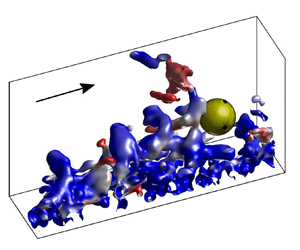
The present data sets enable us to visualize the 3-D vortex structures residing in the TBL using the $Q$-criterion (Hunt, Wray & Moin Reference Hunt, Wray and Moin1988; van Hout et al. Reference van Hout, Eisma, Elsinga and Westerweel2018). An example of a snapshot depicting vortical structures as $Q$-criterion iso-surfaces overlaid with the normalized streamwise and transverse vorticity, $\omega _1^+$ and $\omega _3^+$, is shown in figures 6(a) and 6(b), respectively, while a different viewing angle of the same snapshot is depicted in figure 7. This snapshot shows typical vortical structures residing in the TBL. Note that close to the wall ($x_2^+ \leq 15$), the data are noisy due to the limited spatial measurement resolution. The main vortices prominent in this snapshot are a pair of uplifted, unconnected counter-rotating vortices (denoted ‘SV1’ and ‘SV2’ in figures 6 and 7). The largest of the pair (SV2) exhibits a characteristic ‘cane’ shape (Robinson Reference Robinson1991). SV1 and SV2 are uplifted from the wall at an angle of approximately 40$^\circ$–45$^\circ$, typical of hairpin structures (Adrian Reference Adrian2007). Note that due to the limited transverse extent of the VOI ($\Delta x_3^+ \approx 150$), our measurements do not reveal the complete structure of SV2, or any connection between SV1 and SV2. In addition, in the present data set, we did not observe fully developed, connected hairpin structures likely since typically, they have transverse widths of approximately 100–150 inner wall units (Adrian Reference Adrian2007), i.e. comparable to the width of the VOI. Based on the proximity and similarity of SV1 and SV2, and the fact that they seem to comprise the ‘legs’ of a hairpin structure whose induced flow field ‘ejects’ fluid away from the wall, it is possible that SV1 and SV2 are or were part of a large uplifted hairpin structure. In addition to the uplifted counter-rotating vortical structures, also transverse vortices (such as denoted by ‘TV’ in figures 6 and 7) spanning the width of the VOI were observed. Note that TV is characterized by $\omega _3^+ < 0$ and rotates in the clockwise direction about the $x_3$-axis (as defined for a right-handed Cartesian coordinate system). Just upstream, it ‘sweeps’ fast-moving fluid towards the wall.

Figure 6.

Example snapshot of $Q$-criterion iso-surfaces visualizing the coherent structures detected in the undisturbed TBL. Iso-surfaces are overlaid by (a) the normalized transverse vorticity $\omega _1^+$, and (b) the normalized streamwise vorticity $\omega _3^+$. An animation (supplementary movie 1) depicting the snapshot at different angles is available at https://doi.org/10.1017/jfm.2022.477.

Figure 7.

Same snapshot as depicted in figure 6(b) but at a different viewing angle.

3.2. Sphere dynamics

A total of four spheres, denoted by $S_1$, $S_2$, $S_3$ and $S_4$, were tracked in separate data sets. Their diameters ranged from 7.3 mm to 8.3 mm, and normalized by inner wall scaling were $D^+$ = 66 ($S_1$), 73 ($S_2$), 72 ($S_3$) and 75 ($S_4$). Although only a finite number of spheres were tracked over the entire VOI, their total time trace represents approximately 1000 Kolmogorov time scales.

3.2.1. Sphere translation

The centroid positions of each sphere were tracked in space and time as described in § 2.2, and the normalized wall-normal and transverse sphere centroid positions, $x_{2,c}^+$ and $x_{3,c}^+$, as a function of the sphere's streamwise centroid position $x_{1,c}^+$, are depicted in figure 8. Both the raw and the smoothed data are depicted, showing that smoothing (see § 2.2.2) removes random noise without altering trends. The vertical ‘error’ bar associated with sphere $S_4$ in figure 8(a) indicates its actual size ($D^+ = 75$). The transverse extent of the VOI was in the range 0 $\leq x_3^+ \leq 150$ (the border at $x_3^+ = 0$ is indicated by a horizontal dashed line in figure 8b), and while in most cases the sphere centroid positions were located within the confines of the VOI, $S_1$ and $S_2$ were partially outside of it.

Figure 8.

Sphere wall-normal and transverse centroid positions in inner wall units as functions of $x_{1,c}^+$: (a) $x_{2,c}^{+}$, and (b) $x_{3,c}^{+}$. Red diamonds, $S_1$; blue triangles, $S_2$; black circles, $S_3$; green squares, $S_4$. Open symbols, raw data; filled symbols, smoothed data. Uncertainty is smaller than the marker size. The vertical error bar in (a) at the start of the trajectory of $S_4$ indicates the sphere diameter. The black dashed horizontal line in (b) indicates the edge of the VOI.

Spheres $S_{2}$, $S_{3}$ and $S_{4}$ were located closest to the wall (figure 8a) and moved towards it (all spheres entered the VOI below $x_{2}^{+} = 130$). In contrast, sphere $S_{1}$ (red markers in figure 8a) entered the VOI at $x_{2}^{+}\approx 150$ and remained at almost the same height. We will see in the following sections that the different sphere motion is the result of differences in the flow field in the spheres’ vicinity and consequently different forcing on the spheres. Note that due to their relatively large size, the spheres are mostly immersed in the logarithmic layer, and none of them comes into contact with the wall. Even $S_{3}$ (black markers in figure 8a), which comes closest to the wall ($x_{2,c}^+ = 50$ at $x_{1,c}^+ = 520$; see figure 8a) and almost penetrates the viscous sublayer, is still partially inside the logarithmic layer. As a result, the finite-sized spheres are exposed to different turbulence characteristics in the buffer and the logarithmic layers, and varying velocity gradients act on them. In the transverse direction (figure 8b), $S_{2}$ and $S_{4}$ hardly change position (less than 10 wall units) upon traversing the VOI, while $S_{1}$ and $S_{3}$ exhibit considerable transverse displacements of approximately 40 and 50 wall units ($\sim D^+$), respectively. The latter displacements are approximately 10 % of the corresponding streamwise distance travelled, in agreement with the measurements by Tee et al. (Reference Tee, Barros and Longmire2020). Note that spanwise migration implies spanwise forcing on the sphere, as will be discussed further in § 3.4.

The normalized instantaneous streamwise, wall-normal and transverse sphere centroid velocities are plotted in figures 9 and 10 as functions of $x_{1,c}^+$ for all tracked spheres. Both sphere velocities based on the smoothed centroid positions as well as those based on the derivatives of locally least-squares fitted second-order polynomials are depicted. For comparison, the calculated quiescent settling velocity, $V_s =(\rho _s - \rho )D^2g/(18\mu )$, is also plotted as a horizontal dashed line in figures 9(c,d) and 10(c,d). As expected, the curves of sphere velocities determined based on the derivatives of locally fitted second-order polynomials (solid lines in figures 9 and 10) are smoother than those based on a central difference scheme. However, the trends are conserved. The uncertainties of $V_i^+$ estimated by the r.m.s. values of the difference between $V_{i,c}^+$ based on the raw data and based on the local polynomial fit are presented in the captions of figures 9 and 10.

Figure 9.

Normalized instantaneous sphere centroid velocity components of $S_1$ (a,c,e) and $S_2$ (b,d,f), and the ‘undisturbed’ fluid velocities at the spheres’ centroid positions as functions of $x_{1,c}^+$ in the streamwise (a,b), wall-normal (c,d), and transverse (e,f) directions. $V_i^+$ is based on: squares, smoothed sphere centroid positions; solid curves, derivatives of the least-squares fitted second-order polynomial; triangles, $U_{i,c}^{c+}$; circles, $U_{i,c}^{v+}$. The dashed horizontal line in (c,d) denotes the sphere's settling velocity in a quiescent fluid. Uncertainties of $V_i^+$ estimated by the r.m.s. values of the difference between the sphere centroid velocities based on the raw data and the smoothed (local polynomial fit) data, $\pm ( \delta V_1^+, \delta V_2^+, \delta V_3^+)$, are $(0.39, 0.25, 0.60)$ for $S_1$, and $(0.40, 0.99, 0.49)$ for $S_2$.

Figure 10.

Normalized instantaneous sphere centroid velocity components of $S_3$ (a,c,e) and $S_4$ (b,d,f), and the ‘undisturbed’ fluid velocities at the spheres’ centroid positions as functions of $x_{1,c}^+$ in the streamwise (a,b), wall-normal (c,d), and transverse (e,f) directions. $V_i^+$ is based on: squares, smoothed sphere centroid positions; solid curves, derivatives of the least-squares fitted second-order polynomial; triangles, $U_{i,c}^{c+}$; circles, $U_{i,c}^{v+}$. The dashed horizontal line in (c,d) denotes the sphere's settling velocity in a quiescent fluid. Uncertainties of $V_i^+$ estimated by the r.m.s. values of the difference between the sphere centroid velocities based on the raw data and the smoothed (local polynomial fit) data, $\pm ( \delta V_1^+, \delta V_2^+, \delta V_3^+)$, are $(0.48, 0.19, 0.72)$ for $S_3$, and $(0.26, 0.15, 0.42)$ for $S_4$.

The instantaneous components of the ‘undisturbed’ water velocity vectors $\boldsymbol {U}_c$, based on the two methods discussed in § 2.2, are also plotted in figures 9 and 10. It can be observed that although the two methods lead to slightly different results, overall they compare well. Only for sphere $S_3$ ($U_{1,c}^+$ in figure 10a) and $S_2$ ($U_{1,c}^+$ and $U_{2,c}^+$ in figures 9b,d) are small differences observed, and volume-averaged values of $U^+_{1,c}$ are lower than those interpolated onto the sphere centroid position, and vice versa for $U^+_{2,c}$. This is likely because $S_2$ and $S_3$ were closest to the wall (figure 8a), where the velocity gradients were strongest. Note that in all other cases, values of $U_{i,c}^+$ based on both methods nearly collapse.

Looking at the changes in $V_1^+$ (figures 9a,b and 10a,b), it is observed that only for $S_3$ (figure 10a) does $V_1^+$ decrease upon approaching the wall from about $V^+_1 \approx 16.5$ at $x_{1,c}^+ = 50$ ($x_{2,c}^+ \approx 94)$ to $V_1^+\approx 15$ at $x_{1,c}^+\approx 500$ ($x_{2,c}^+ \approx 51)$. The corresponding values of the undisturbed average streamwise water velocity (figure 4) are similar and are given by $\langle \bar {U}_1\rangle ^+ = 14.6$ and 16.1 at $x_2^+ = 51$ and 93, respectively. In contrast, $S_2$ and $S_4$, which also move towards the wall (figure 8a), have nearly constant $V_1^+$ – i.e. $V_1^+ \approx 17.2$ and 17.0 for $S_2$ and $S_4$, respectively – and they move faster than the mean water flow at the same height (figure 4) for most of their trajectory. Only $S_1$, which moves slightly away from the wall (figure 8(a), $x_{2,c}^+ \approx 150$), increases its streamwise velocity from $V_1^+ \approx 15$ to $V_1^+ \approx 16$ (figure 9a), moving slower than the mean water velocity at this height ($\langle \bar {U}_1\rangle ^+ = 17.2$ at $x_{2,c}^+ = 150$; figure 4). Note that $S_{1}$, which enters the VOI farthest from the wall, has a streamwise velocity that is lower than those of $S_{2}$, $S_{3}$ and $S_{4}$ (figures 9a,b and 10a,b). Based on the mean streamwise water velocity profile (see figure 4) and the sphere's wall-normal position, one would expect it to be advected at a higher velocity. However, since $-\langle \overline {u_1u_2}\rangle ^+ > 0$ (see figure 5c), a negative correlation between $u_1$ and $u_2$ dominates, and $S_1$ is advected by relatively slow-moving fluid as indicated by the accompanying values of $U_{1,c}^+$.

Streamwise velocity components of $S_1$ and $S_3$ (figures 9a and 10a) clearly lag the interpolated ‘undisturbed’ water velocities along the trajectories, resulting in a drag force acting on the sphere in the streamwise direction, as will be discussed in § 3.4. Note that only in the case of $S_1$ (figure 9b) does $V_2^+$ lag $U_{2,c}^+$ along its trajectory, resulting in an upward-directed drag force (see § 3.4) inhibiting wall-ward motion (figure 8a). In all other cases, values of $V_i^+$ fluctuate around those of $U_{i,c}^+$. An indication of the differences between the sphere and fluid velocities at the sphere's position is provided by the r.m.s. values of $U_{i,r}^+$ ($= V_i^+ - U_{i,c}^{v+}$, with $V_i^+$ based on the smoothed data) and the averages along the sphere trajectories, $\bar {U}_{i,r}^+$, as summarized in table 1 for the different spheres. Values of $\bar {U}_{1,r}^+$ show that on average, in all cases the spheres lag the fluid, while in the transverse and wall-normal directions, this is not necessarily the case. Further note that similar magnitudes of $( U^+_{1,r})^\prime$ and $\bar {U}_{1,r}^+$ indicate that the spheres either lag ($\bar {U}_{1,r}^+ < 0$) or exceed ($\bar {U}_{1,r}^+ > 0$) the fluid for most of their trajectories.

Table 1.

Summary of the values of $( U^+_{i,r})^\prime$ and $\bar {U}_{1,r}^+$ for all investigated spheres.

The instantaneous wall-normal velocities of the spheres (figures 9c,d and 10c,d) are in accordance with the direction of their wall-normal motion (see figure 8a), i.e. for $S_1$, $V_2^+ > 0$, and in all other cases, $V_2^+ < 0$. Another interesting point to notice is that for the spheres that move towards the wall ($S_{2}$, $S_{3}$ and $S_{4}$), $|V_2^+| \approx 0.5|U_s|$, indicating that besides the net buoyancy force, additional forces opposing gravity, such as drag and lift forces, must be important, as will be discussed further in § 3.4. Note that this result is different from measurements reported by Tee et al. (Reference Tee, Barros and Longmire2020), who found that wax spheres ($D^+ = 58 \pm 2$, $\rho _s/\rho = 1.006 \pm 0.003$) with characteristics similar to those of the present hydrogels, suspended in a TBL ($Re_\tau = 680$), descended at almost $2|U_s|$. Physically, this means that the spheres must be exposed to a significant downward fluid impulse that was not observed for the spheres investigated here.

The magnitudes of $V_3^+$ (figures 9e,f and 10e,f) are of the same order of magnitude as those of $V_2^+$ (figures 9c,d and 10c,d). In accordance with their spanwise displacement (figure 8b), spheres $S_{1}$ and $S_{3}$ exhibited higher values of $|V_3^+|$ (figures 9e and 10e) than spheres $S_2$ and $S_4$, for which $V_3^+ \approx 0$ (figures 9f and 10f). Our results indicate that spanwise motion may be significant and should not be neglected, in agreement with Tee et al. (Reference Tee, Barros and Longmire2020).

In all cases, it can be observed in figures 9 and 10 that the sphere velocities exhibit fluctuations along their tracks with amplitudes exceeding the estimated uncertainties (see captions of figures 9 and 10). The estimated frequencies $f_i$ ($i = 1,2,3$), and Strouhal numbers based on the r.m.s. values of the components of the relative velocities, $Sr_i = f_iD/(U_{i,r}^v)^\prime$ ($i = 1,2,3$), are summarized in table 2. Note that Tee et al. (Reference Tee, Barros and Longmire2020) also reported sphere velocities that fluctuated, which they attributed to vortex shedding ($Re_s > 100$). In the present case, Strouhal numbers are much higher than those associated with vortex shedding in the wake of a sphere in a uniform flow ($0.1< Sr < 0.2$). Note that Tee et al. (Reference Tee, Barros and Longmire2020) did not measure the instantaneous flow field in the vicinity of the spheres, and their Strouhal numbers were based on the mean, ‘undisturbed’ streamwise water velocity at the sphere's centroid position. This will overestimate $Re_s$ and result in lower $Sr$ than when the actual slip velocity is accounted for. In the present measurements, the instantaneous sphere Reynolds numbers $Re_s = |{\boldsymbol U}_r|D/\nu$, based on the magnitude of the instantaneous relative velocity vector, is mostly in the range $10 \leq Re_s \leq 80$ (see figure 11), while $\overline {Re}_s = 63$, 36, 31 and 35 for $S_1$, $S_2$, $S_3$ and $S_4$, respectively. Since for spheres exposed to a uniform flow, flow separation occurs at $Re_s \approx 25$ (Taneda Reference Taneda1956), small wake oscillations start at $Re_s \approx 130$, and unsteady vortex shedding starts at $Re_s \approx 270$ (Sakamoto & Haniu Reference Sakamoto and Haniu1990), it is unlikely that vortex shedding played a role here. However, flow separation may occur, and in conjunction with the unsteady TBL flow might lead to oscillations in sphere velocities. Furthermore, as a result of the surrounding turbulence, the onset of flow separation and vortex shedding may occur at a lower $Re_s$ value. However, we did not observe any signs of this in the measured 3-D flow field as discussed further in § 3.4.

Figure 11.

Histograms of the instantaneous sphere Reynolds numbers, $Re_s$, for all four spheres. Data points are located at the centres of the bins (bin size 10).

Table 2.

Summary of the estimated frequencies $f_i$ and Strouhal numbers $Sr_i = f_iD/(U_{i,r}^v)^\prime$ associated with the fluctuating sphere velocities.

Another mechanism that may lead to fluctuations in sphere velocities is the forcing provided by the turbulence in the vicinity of the spheres. The turbulence time scales can be estimated based on (i) the viscous time scale $\tau _v = \nu /u_\tau ^2$, and (ii) the Kolmogorov time scale $\tau _k = (\nu /\epsilon )^{1/2}$, where $\epsilon$ is the turbulent kinetic dissipation rate that can be estimated in the log layer by $\epsilon \approx \overline {u_1u_1}({\partial \bar {U}_1}/{\partial x_2}) /3$ (Pope Reference Pope2000). Based on the present data (summarized in table 3), this leads to $f_v (= 1/\tau _v) = 81$ Hz, and $f_k (= 1/\tau _k) = 22$ and 12.7 Hz at $x_2^+ = 50$ and 100, respectively. Although these are crude estimates, the $f_i$ (table 2) are of the same order of magnitude as $f_v$ and $f_k$, supporting our hypothesis. Note further that we validated that these frequencies were not an artefact of the applied local regression detailed in § 2.2.

Table 3.

Summary of the estimated scales in the log layer.

3.2.2. Sphere rotation

The angular velocities of the sphere, $\dot {\alpha }_i$, were determined by the ICP algorithm as described in § 2.2. Based on the interpolated water velocity vector field (see § 2), the streamwise, wall-normal and transverse components of ${\boldsymbol \omega }_c$ were calculated and similar as for $\boldsymbol U_c$, ${\boldsymbol \omega }_c$ was evaluated as the volume-averaged value at the sphere's centroid. The components of the water angular velocities based on ${\boldsymbol \omega }_c$ and normalized in inner wall scaling are given by $\varOmega _{i,c}^+ = (\omega _{i,c}\nu )/(2u_\tau ^2)$, while the normalized angular sphere velocities are given by $\dot \alpha _i^+ = (\dot \alpha _i\nu )/u_\tau ^2$ ($i = 1,2,3$).

The results for $\dot \alpha _i^+$ (smoothed), $\varOmega _{i,c}^{v+}$ and $\varOmega _{i,c}^{c+}$ are plotted in figures 12 and 13 as functions of $x_{i,c}^+$ for spheres $S_1, S_2$ and $S_3, S_4$, respectively. Average values of $\dot \alpha _i^+$ and $\varOmega _{i,c}^{v+}$ are summarized in table 4. All four spheres exhibited negative (clockwise) angular velocities about the $x_3$-axis ($\dot \alpha _3^+ < 0$, figures 12a,b and 13a,b, and $\overline {\dot \alpha _3^+} < 0$ in table 4) in accordance with the positive mean shear rate near the wall. Water angular velocity components mostly have the same signs as those of the spheres, and in most cases the rotational motion of the spheres lags that of the fluid (see table 4). Values of $\varOmega _{i,c}^{v+}$ clearly differ in magnitude from $\varOmega _{i,c}^{c+}$, especially for rotation about $x_3$ (figures 12a,b and 13a,b), and in most cases, $\varOmega _{i,c}^{v+} < \varOmega _{i,c}^{c+}$. This is the result of significant spatial non-uniformity of the vorticity at the sphere's position as it is immersed in the buffer and log layer of the TBL, where turbulence is most active. In the case of high spatial non-uniformity, and taking the finite size of the spheres into account, one may argue that the volumetric mean presents a better estimate than the value evaluated at the sphere centroid. Sphere $S_3$, which is located closest to the wall, has the highest magnitude of $\overline {\dot \alpha _3^+}$, followed by $S_1$, while $S_2$ and $S_4$ rotate the slowest about $x_3$ (see table 4). Note that the importance of the combined shear-, wall- and rotation-induced lift forces on the wall-normal motion of the spheres is discussed further in § 3.4.

Figure 12.

Instantaneous normalized angular velocities of the sphere and the water versus $x_{1,c}^{+}$ for $S_1$ (a,c,e) and $S_2$ (b,d,f). Squares indicate sphere angular velocities $\dot \alpha ^+_i$ based on smoothed data. Water angular velocities at the sphere position are given for: $\varOmega _{i,c}^{v+}$, circles; and $\varOmega _{i,c}^{c+}$, triangles. Rotation is about: (a,b) $x_3$, (c,d) $x_2$, (e,f) $x_1$.

Figure 13.

Instantaneous normalized angular velocities of the sphere and the water versus $x_{1,c}^{+}$ for $S_3$ (a,c,e) and $S_4$ (b,d,f). Squares indicate sphere angular velocities $\dot \alpha ^+_i$, based on smoothed data. Water angular velocities at the sphere position are given for: $\varOmega _{i,c}^{v+}$, circles; and $\varOmega _{i,c}^{c+}$, triangles. Rotation is about: (a,b) $x_3$, (c,d) $x_2$, (e,f) $x_1$.

Table 4.

Summary of angular sphere and water velocities averaged over the spheres’ trajectories.

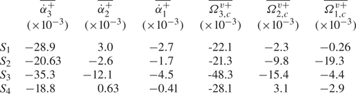
In all cases, sphere angular velocities about the $x_1$- and $x_2$-axes ($\dot \alpha ^+_1$ and $\dot \alpha ^+_2$ in figures 12 and 13) are small, and mean values are substantially smaller than those about the $x_3$-axis (see table 4). Only for $S_3$ is $\overline {\dot \alpha ^+_2}$ significant ($\approx 0.3\overline {\dot \alpha ^+_3}$; see table 4) and the importance of the rotation-induced lift force acting in the transverse direction (see figure 8b) will be discussed in § 3.4. The mean values of the relative angular velocities along the different sphere tracks, $\overline {\varOmega _{i,r}^{v+}} = \overline {\dot \alpha _i^+ - \varOmega ^{v+}_{i,c}}$ ($i = 1,2,3$) including their standard deviations, are summarized in table 5. Values illustrate that the $\overline {\varOmega _{i,r}^{v+}}$ vary significantly for the different spheres and display large standard deviations as a result of the different flow field characteristics in their immediate vicinity that are discussed next.

Table 5.

Summary of the average values of the relative angular velocities. Standard deviations are depicted as uncertainties.

3.3. Flow field in the vicinity of the spheres

The present measurements allow us to determine simultaneously the instantaneous flow field in the vicinity of the spheres as well as their motion (see §§ 3.2.2 and 3.2.1). Since spheres $S_3$ and $S_4$ were fully resolved within the VOI (see figure 8), we will focus on them in this subsection.

3.3.1. Sphere $S_3$

Two instantaneous snapshots ($\Delta t^{+}=16.7$) of sphere $S_3$, including the instantaneous vortices overlaid by $\omega _1^+$, are presented in figure 14 (and animations are provided in supplementary movie 2). As observed, $S_{3}$ is surrounded by a plethora of vortical structures. A group of fragmented transverse and inclined vortices within the dashed ellipse in figure 14(a) can be observed just upstream of $S_3$ upon entering the VOI. The inclination angle of this group is approximately 40 $^\circ$ from the bottom wall, agreeing well with typical inclination angles of hairpin packets observed in TBLs (Adrian Reference Adrian2007). However, no complete connected hairpin structures were observed. As the sphere traverses the VOI (figure 14b), most transverse vortices associated with the packet leave the VOI, and mainly streamwise-oriented longitudinal vortices rotating about the $x_1$-axis are observed (figure 14b). In particular, close to the wall just below and downstream of $S_3$, two counter-rotating longitudinal vortices denoted by ‘LV1’ ($\omega _1^+ > 0$) and ‘LV2’ ($\omega _1^+ < 0$) can be discerned in figure 14. They are located close to the wall inside the buffer layer ($x_2^+ < 50$) and extend up to $x_1^+ \approx 300$ in figure 14(a).

Figure 14.

Two snapshots ($\Delta t^{+}=16.7$) of the instantaneous vortical structures in the vicinity of $S_{3}$ visualized by $Q$-criterion iso-surfaces overlaid by $\omega _1^+$. The sphere's surface is depicted in yellow, with black markers to indicate its change in orientation. Values in parentheses denote $(x_{1,c}^+, x_{2,c}^+, x_{3,c}^+)$. Supplementary movie 2 provides animations of the snapshot in (a) at different viewing angles.

A close up of the sphere and parts of LV1 and LV2 are depicted in figure 15 at different viewing angles, revealing some interesting characteristics. First, LV1 and LV2 are not connected. Instead, just upstream of $S_3$, a transverse ‘bridging’ vortex located between $x_1^+ = 50$ and 80 (denoted ‘TV1’ in figure 15) connects to LV1 and extends in the negative $x_3^+$-direction up to the edge of the VOI ($x_3^+ = 0$). This suggests that LV1 and TV1 are part of a hairpin-like structure (Adrian Reference Adrian2007). Note that also LV2 is connected to a transverse vortical structure (denoted ‘TV2’ in figure 15) extending up to the edge of the VOI in the positive $x_3^+$ direction. The rotation directions of LV1, LV2, TV1 and TV2 that are indicated by the overlaid streamwise and transverse normalized vorticity components in figures 15(a) and 15(b), respectively, indicate that they generate downward-moving fluid just ahead of the sphere. This downward motion is responsible for the relatively strong wall-ward motion of $S_3$ (see figure 8(a) as well as figures 9 and 10).

Figure 15.

Close-up of the snapshot of sphere $S_3$ in figure 14(a) at two different viewing angles. Vortical structures are visualized by $Q$-criterion iso-surfaces overlaid by (a) $\omega _1^+$, and (b) $\omega _3^+$. The sphere surface is depicted in yellow, with black markers indicating its orientation.

This is investigated further by analysing snapshots ($\Delta t^+$ = 5.5) of equatorial wall-normal ($x_1\unicode{x2013}x_3$) and wall-parallel ($x_1\unicode{x2013}x_2$) planes moving with the sphere that depict the instantaneous correlations of water fluctuating velocities, $(u_1u_2)^+$ (figures 16a,c,e,g and 17a,c,e,g). Here and in similar plots subsequently, the sphere's cross-section is indicated by a white circle, and its rotation in the depicted plane relative to its initial orientation (denoted by a dashed line) is indicated by a rotated solid line extending from the sphere's centre. Contour plots of $(u_1u_2)^+$ (figures 16a,c,e,g and 17a,c,e,g) clearly show a large, highly coherent area where $(u_1u_2)^+ < 0$ just downstream of the sphere. Negative values of $(u_1u_2)^+$ may indicate both sweeps and ejections, and to determine to which quadrant they belong, contour plots of $u_1^+$ in the same equatorial planes are depicted in figures 16(b,d,f,h) and 17(b,d,f,h). Combining the plots of $(u_1u_2)^+$ and $u_1^+$, it becomes clear that just downstream of the sphere, the area associated with $(u_1u_2)^+ < 0$ correlates with $u_1^+ >0$, indicating that sweeps induced by the combined action of the coherent structures (figures 14 and 15) dictate the flow field just downstream of $S_3$.

Figure 16.

For $S_{3}$, a sequence ($\Delta t^{+}=5.5$) of equatorial wall-normal planes depicting the correlations of instantaneous water fluctuating velocities $(u_1u_2)^+$ (a,c,e,g), and the streamwise water velocity fluctuating velocities $u_1^+$ (b,d,f,h). The hydrogel sphere is depicted as a filled white circle. Its initial orientation is indicated by a dashed line, while its changing orientation is indicated by a solid line.

Figure 17.

For $S_{3}$, a sequence ($\Delta t^{+}=5.5$) of equatorial wall-parallel planes depicting the correlations of the instantaneous water fluctuating velocities $(u_1u_2)^+$ (a,c,e,g), and the streamwise water fluctuating velocities $u_1^+$ (b,d,f,h). The hydrogel sphere is superposed as a filled white circle. Its initial orientation is indicated by a dashed line, while its changing orientation is indicated by a solid line. Note that the view is from the wall upwards.

Besides the coherent sweep motion just downstream of $S_3$, it can be seen in the wall-parallel equatorial planes (figures 17b,d,f,h) that $S_{3}$ is exposed to transverse shear. This is especially clear in figures 17(d,f), where patches of positive and negative streamwise velocity fluctuations on opposite sides of $S_3$ are observed. The resulting shear-induced lift force will be discussed in § 3.4.

3.3.2. Sphere $S_4$

Similarly as for $S_3$, three snapshots ($\Delta t^+$ = 13.7) of the vortices in the vicinity of $S_4$ are depicted as $Q$-criterion iso-surfaces in figure 18, overlaid by $\omega ^+_1$ and by $\omega _3^+$. Also in this case, several vortical structures characteristic of TBLs can be discerned. In particular, downstream of $S_4$, two counter-rotating, uplifted longitudinal vortices (denoted by ‘LV3’ and ‘LV4’ in figure 18) can be seen. LV4 is positioned above LV3 (see supplementary movies 3 and 4), and both are tilted with respect to the $x_1^+$-axis towards the $x_3^+$-axis. As $S_4$ traverses the VOI, downstream of it, a well-defined hairpin packet appears, consisting of four hairpin heads (denoted by ‘HP1’ to ‘HP4’ in figures 18b,c). Again due to the limited transverse extent of the VOI, only a part of the packet is resolved. All the hairpin heads rotate in the clockwise direction ($\omega _3^+ < 0$; figure 18c), in agreement with the direction of the mean shear. Note that the sphere is not overtaken by the hairpin packet as reported by van Hout (Reference van Hout2013), who studied smaller ($D^+ \approx 10)$ polystyrene beads, but instead remains positioned just upstream of the identified hairpin packet. However, it seems that the hairpin packet's development is hampered as $S_4$ moves towards the wall. Evidence for this can be found by looking at a close-up of the vortices in the vicinity of $S_4$ as shown in figure 19. This close-up shows that a somewhat distorted hairpin vortex is located below $S_4$ (denoted by ‘HP5’ in figure 19), and it is likely that HP5 is part of the identified hairpin packet upstream of $S_4$. However, the wall-ward motion of $S_4$ hinders the self-induced upward motion of HP5, and ‘pushes’ HP5 towards the wall. Note further that the ‘legs’ of HP5 generate ejection motion that may explain why $S_4$ settles slightly slower than $S_3$ (see figure 10).

Figure 18.

Sequence of instantaneous vortical structures (visualized by $Q$-criterion iso-surfaces) in the vicinity of sphere $S_4$ ($\Delta t^{+}=16.7$). Iso-surfaces were overlaid by (a,b) $\omega _1^+$, and (c) $\omega _3^+$. The hydrogel sphere is depicted in yellow with black markers to indicate its change in orientation. The values in parentheses denote $(x_{1,c}^+, x_{2,c}^+, x_{3,c}^+)$. Supplementary movies 3 and 4 provide animations of the snapshots in (b,c) at different viewing angles.

Figure 19.

Close-up of vortical structures in the vicinity of $S_4$. Vortical structures were visualized by $Q$-criterion iso-surfaces that were overlaid by $\omega _1^+$. Snapshots in (a,b) correspond to figures 18(a,b).

Wall-normal and wall-parallel equatorial planes depicting contour plots of $(u_1u_2)^+$ and $u_1^+$ are presented in figures 20 and 21. Similarly as for $S_3$, also downstream of $S_4$ a distinct sweep (denoted by ‘SW’ in figure 20) is observed, most likely induced by LV4 (figure 18b). In addition, below SW and slightly downstream of it close to the wall, a clear ejection (denoted by ‘EJ’ in figure 20a) is seen. As $S_4$ traverses the VOI, it stays just upstream of the sweep (located just downstream of the slanted dashed line across figures 20a,c,e,g). Further note that the ‘signature’ of the hairpin packet (see figure 18c) becomes visible as a train of uplifted opposite sign patches of $u_1^+$ (dashed ellipse in figure 20l) induced by the hairpin heads HP1 to HP4 (figure 18c).

Figure 20.

For $S_{4}$, a sequence ($\Delta t^{+}=4.9$) of equatorial wall-normal planes depicting the correlations of the instantaneous water fluctuating velocities $(u_1u_2)^+$ (a,c,e,g,i,k), and the streamwise water fluctuating velocities $u_1^+$ (b,d,f,h,j,l). The hydrogel sphere is superposed as a filled white circle. Its initial orientation is indicated by a dashed line, while its changing orientation is indicated by a solid line. ‘SW’ and ‘EJ’ in (a) denote sweep and ejection motion, respectively. The slanted dashed line across (a,c,e,g) demarcates the upstream position of a sweep motion.

Figure 21.

For $S_{4}$, a sequence ($\Delta t^{+}=4.9$) of equatorial wall-parallel planes depicting the correlations of the instantaneous water fluctuating velocities $(u_1u_2)^+$ (a,c,e,g,i,k), and the streamwise water fluctuating velocities $u_1^+$ (b,d,f,h,j,l). The hydrogel sphere is superposed as a filled white circle. Its initial orientation is indicated by a dashed line, while its changing orientation is indicated by a solid line. A progressing sweep motion (SW) can be seen between the two parallel dashed lines in (a–h). Note that the view is from the wall upwards.

3.4. Lift and drag forces acting on the spheres

Sphere motion is dictated ultimately by the forces acting on it, amongst them the lift and drag forces that we focus on in this subsection. Inertial forces such as the fluid pressure, the Basset history force, and the added mass forces and their importance will be discussed at the end of this subsection. For the present range of $Re_s$ (figure 11), the drag force acting on the spheres can be calculated by the quadratic drag relation given by (e.g. Yam et al. Reference Yam, Burns, Ingham and McCaffrey2013)

(3.1)\begin{equation} \boldsymbol{F}_D ={-}C_D\,\frac{1}{2}\,\rho\,\frac{{\rm \pi} D^2}{4}\,|\boldsymbol{U}_r|\,\boldsymbol{U}_r, \end{equation}

where $C_D$ denotes the drag coefficient for spheres. In the present case, due to the effect of shear and wall proximity, as well as ambient turbulence (Zeng et al. Reference Zeng, Najjar, Balachandar and Fischer2009), $C_D$ may be modified from the standard drag relation $C_{Do} = ({24}/{{Re}_s}) (1 + 0.15{Re}_s^{0.687})$ (Schiller–Naumann correlation, valid for $0.01 < {Re}_s < 1000$; Clift, Grace & Weber Reference Clift, Grace and Weber1978). Zeng et al. (Reference Zeng, Najjar, Balachandar and Fischer2009) and Shi et al. (Reference Shi, Rzehak, Lucas and Magnaudet2021) have proposed correlations for the drag and lift coefficients based on direct numerical simulations (DNS) studies of a stationary sphere in a wall-bounded linear shear flow and of a rigid sphere translating steadily near a wall, either in a fluid at rest or in the presence of a uniform shear, respectively. While the DNS by Shi et al. (Reference Shi, Rzehak, Lucas and Magnaudet2021) may be more relevant to the present study, their correlations are valid within a narrow range of the relative shear rate, $-0.5 \leq Sr\ (= (\partial U_1/\partial x_2)_cD/|\boldsymbol {U}_r|) \leq 0.5$. In the case when $|\boldsymbol {U}_r|$ becomes small, such as for nearly neutrally buoyant particles, magnitudes of $Sr$ exceed this range easily. This is the case in the present study, where $|\boldsymbol {U}_r|$ is small, and values of $|Sr|$ are an order of magnitude higher than the range for which the correlations proposed by Shi et al. (Reference Shi, Rzehak, Lucas and Magnaudet2021) are valid. Although maximum values in Zeng et al. (Reference Zeng, Najjar, Balachandar and Fischer2009) are also bounded by $Sr = 2$, their correlations do not contain $Sr$ explicitly. We therefore used the correlations proposed by Zeng et al. (Reference Zeng, Najjar, Balachandar and Fischer2009) for the calculation of the lift and drag coefficients. Taking shear and wall proximity into account, Zeng et al. (Reference Zeng, Najjar, Balachandar and Fischer2009) proposed the following correction to standard drag for a stationary sphere in a wall-bounded, linear shear flow:

(3.2)\begin{equation} C_D = C_{Do}(1+\alpha\,Re_s^\beta), \end{equation}

where $\alpha = 0.15-0.046(1-0.16\delta ^2)\exp (-0.7\delta )$, with the normalized sphere-to-wall gap given by $\delta = x_{2,c}/D - 0.5$, and $\beta = 0.687 + 0.066(1-0.76\delta ^2) \exp (-\delta ^{0.9})$. Note that when $\delta \rightarrow \infty$, $C_D = C_{Do}$.

Besides the drag, the lift force acting perpendicular to it may be of importance. However, in contrast to the drag, there is significant uncertainty regarding the validity of lift force correlations. In the Stokes limit, no lift forces act on the sphere even in the presence of a wall (Bretherton Reference Bretherton1962). However, in the present measurements, Stokes flow cannot be assumed, and lift forces may play a role (see figure 11). For a rotating sphere in a shear flow close to a wall (Zeng et al. Reference Zeng, Najjar, Balachandar and Fischer2009), shear-induced, rotation-induced (so-called ‘Magnus’ force) and wall-induced lift forces may all be important. Starting with the early studies by Segre & Silberberg (Reference Segre and Silberberg1962) and Saffman (Reference Saffman1965) for low $Re_s$ and low shear rates, the shear-induced lift force has been a topic of investigation for many decades (see Zeng et al. Reference Zeng, Najjar, Balachandar and Fischer2009; Shi & Rzehak Reference Shi and Rzehak2019, Reference Shi and Rzehak2020). Correlations valid for extended ranges of $Re_s$ and shear rate magnitude have been proposed (see recent reviews by Shi & Rzehak Reference Shi and Rzehak2019, Reference Shi and Rzehak2020).

In analogy with the drag force (3.1), the shear-induced lift force acting on the sphere can be determined by

(3.3)\begin{equation} \boldsymbol{F}_L^S = C_L^S \rho\,\frac{\rm \pi}{8}\,D^2 \left |\boldsymbol{U}_r\right|^2\boldsymbol{e}_{{\perp}\varOmega}, \end{equation}

where $C_L^S$ denotes the shear-induced lift coefficient (indicated by the superscript ‘$S$’), and $\boldsymbol {e}_{\perp \varOmega }$ is the unit vector in the direction of $(\boldsymbol {\varOmega }\times \boldsymbol {U}_r)$, where ‘$\times$’ denotes the cross product. An expression similar to (3.3) may be used for the wall-induced lift (superscript ‘$W$’), albeit with a different lift coefficient, $C_L^W$ (Shi & Rzehak Reference Shi and Rzehak2020). In addition to the shear and wall-induced lift forces, the Magnus force (based on inviscid flow analysis) can be determined by

(3.4)\begin{equation} \boldsymbol{F}_L^R = C_L^R\rho\,\frac{\rm \pi}{8}\,D^2 \left |\boldsymbol{U}_r\right|^2\boldsymbol{e}_{{\perp}\dot{\alpha}}, \end{equation}

where $C_L^R$ denotes the rotation-induced lift coefficient (denoted by the superscript ‘$R$’), and $\boldsymbol {e}_{\perp \dot {\alpha }}$ is the unit vector in the direction of $(\boldsymbol {\dot \alpha }\times \boldsymbol {U}_r)$.

Care must be taken with regard to the sign of the lift forces since it depends on whether viscous or inviscid lift mechanisms dominate. The direction of the Magnus force (inviscid case) is always towards the advancing side of the sphere. However, with viscous effects taken into account, boundary layer growth and separation may be different along the advancing and retreating sphere surfaces, thereby reversing the direction of the Magnus force (the so-called ‘inverse’ Magnus effect; Kim et al. Reference Kim, Choi, Park and Yoo2014). As outlined by Kim et al. (Reference Kim, Choi, Park and Yoo2014), the inverse Magnus effect occurs at high Reynolds numbers (${\sim }10^5$) and is not expected to play a role here.

As seen in (3.3), the direction of $\boldsymbol {F}_L^S$ is perpendicular to $(\boldsymbol {\varOmega }\times \boldsymbol {U}_r)$, which means that in a wall-bounded linear shear flow, it depends on the sign of $\boldsymbol {U}_r$ (Shi & Rzehak Reference Shi and Rzehak2020), i.e. $\boldsymbol {F}_L^S$ may be either positive (directed away from the wall when $\boldsymbol {U}_r < 0$) or negative (directed towards the wall when $\boldsymbol {U}_r > 0$). Also, the wall-induced lift force may be directed towards or away from the wall depending on the relative dominance of viscous or inviscid lift mechanisms (see Zeng et al. Reference Zeng, Najjar, Balachandar and Fischer2009). Furthermore, DNS studies showed that the sign of $\boldsymbol {F}_L^S$ is a function of $Re_s$ (Kurose & Komori Reference Kurose and Komori1999; Zeng et al. Reference Zeng, Najjar, Balachandar and Fischer2009; Shi & Rzehak Reference Shi and Rzehak2019), i.e. when $Re_s > 55$ flow separation resulted in asymmetrical distributions of pressure and viscous stresses, and the lift force became negative (see also Kurose & Komori Reference Kurose and Komori1999; Zeng et al. Reference Zeng, Najjar, Balachandar and Fischer2009; Shi & Rzehak Reference Shi and Rzehak2019). Negative lift has also been observed in the vicinity of a wall and is strongest when the sphere is located about one diameter from it (Zeng et al. Reference Zeng, Najjar, Balachandar and Fischer2009).

Based on DNS studies, a correlation for the shear-induced lift coefficient for a stationary sphere in a wall-bounded linear shear flow has been proposed by Zeng et al. (Reference Zeng, Najjar, Balachandar and Fischer2009):

(3.5)\begin{equation} C_L^S = C_{L,w}^S\exp({-}0.5\delta({Re}_s/250)^{4/3})\left[\exp(\alpha_L^S\delta^{\beta_L^S})-\lambda_L^S\right], \end{equation}

where $\alpha _L^S = -\exp (-0.3+0.025Re_s)$, $\beta _L^S = 0.8 + 0.01Re_s$, and $\lambda _L^S = (1 - \exp (-\delta ))$ $(Re_s/250)^{5/2}$; here, $C_{L,w}^S = 3.663/(Re^2_s + 0.1173)^{0.22}$ denotes the lift coefficient in the limit of the sphere touching the wall (denoted by the subscript ‘$w$’). Equation (3.5) is valid in the range $1 < Re_s < 200$. Note that the correlation for $C_L^S$ (3.5) does also include the effect of wall proximity, which reduces with increasing $\delta$ (see Zeng et al. Reference Zeng, Najjar, Balachandar and Fischer2009). Therefore, in the present case, values of $C_L^S$ according to (3.5) are enhanced over their unbounded counterparts. A correlation for the wall-induced lift coefficient on a sphere moving parallel to a wall in a quiescent fluid is given by (Zeng et al. Reference Zeng, Najjar, Balachandar and Fischer2009)

(3.6)\begin{equation} C_L^W = f + \left[C_{L,w}^W - f_{x_{2,c}/D=1/2}\right]\exp\left[{-}11(\delta/\delta_c)^{1.2}\right], \end{equation}

where $\delta _c = 3\exp (-0.17 Re_s^{0.7})$, and $f(x_{2,c}/D, Re_s) = (1+0.329Re_s + 0.00485Re_s^2)$ $C_{L,w}^W (x_{2,c}/D)^{[-0.9\,{\rm tanh}(0.022{Re}_s)]}$. The wall-induced lift coefficient for a sphere touching the wall is given by $C_{L,w}^W = (9/8 + 5.78\times 10^{-6}({Re}_s\,x_{2,c}/D)^{4.58}) \exp (-0.292{Re}_s\,x_{2,c}/D)$ for $0 < {Re}_s\,x_{2,c}/D < 10$, and $C_{L,w}^W = 8.94({Re}_s\,x_{2,c}/D)^{-2.09}$ for $10 < {Re}_s\,x_{2,c}/D < 300$ (Takemura & Magnaudet Reference Takemura and Magnaudet2003). Finally, a correlation for the rotation-induced lift coefficient was adopted from Bagchi & Balachandar (Reference Bagchi and Balachandar2002):

(3.7)\begin{equation} C_{L,i}^R \approx{-}0.55 \dot\alpha_3 D/|\boldsymbol{U}_r|. \end{equation}

Note that only the correlation for $C_L^S$ (see (3.5)) takes flow separation into account, and the sign of $C_L^S$ may be reversed (negative lift) depending on $Re_s$.

The additive nature of the different contributions to the lift force has been investigated by Bagchi & Balachandar (Reference Bagchi and Balachandar2002), Zeng (Reference Zeng2007) and Bluemink et al. (Reference Bluemink, Lohse, Prosperetti and Van Wijngaarden2008). Zeng (Reference Zeng2007) showed that linear superposition of wall and shear contributions is incorrect and underestimates the actual lift coefficient especially when close to the wall ($2x_{2c}/D \leq 2$; Shi et al. Reference Shi, Rzehak, Lucas and Magnaudet2021) and for low $Re_s$ ($1 \leq Re_s \leq 100$; see also Shi et al. Reference Shi, Rzehak, Lucas and Magnaudet2021). However, combined wall and shear contributions (superimposed nonlinearly) do superimpose linearly with the rotational contribution to the total lift coefficient (Shi et al. Reference Shi, Rzehak, Lucas and Magnaudet2021), in agreement with Bagchi & Balachandar (Reference Bagchi and Balachandar2002) and Bluemink et al. (Reference Bluemink, Lohse, Prosperetti and Van Wijngaarden2008), who concluded that the total lift force on a freely rotating sphere in a shear flow ($0 < Re_s \leq 200$) can be taken as the superposition of the lift on a stationary sphere in a shear flow (3.3) and the lift on a sphere forced to spin at the torque-free rotation rate in a uniform flow. As shown by Bagchi & Balachandar (Reference Bagchi and Balachandar2003), freestream turbulence did not have a substantial effect on the time-averaged drag that could be determined accurately by the standard drag relation. However, accurate prediction of the instantaneous drag deteriorated with increasing particle size. Once vortex shedding occurred for $Re_s > 270$ (Bagchi & Balachandar Reference Bagchi and Balachandar2003), the effect of isotropic freestream turbulence on the lift forces appeared to be minor. Note that the effect of non-isotropic ambient turbulence such as in a TBL has not been studied (see Shi & Rzehak Reference Shi and Rzehak2020), and it is unclear if the available correlations are valid for spheres immersed in a TBL. Therefore, magnitudes of the drag and lift forces calculated here must be interpreted with caution.

In the absence of gravitation, the lift and drag forces are expected to be important for sphere motion in the transverse plane, where especially $S_1$ and $S_3$ exhibit strong transverse motion in opposite directions (figure 8b). The instantaneous transverse components of $\boldsymbol {F}^R_L$, $\boldsymbol {F}^S_L$, $\boldsymbol {F}^W_L$ and $\boldsymbol {F}_D$ calculated by (3.1)–(3.7), and normalized by $\rho \nu ^2$, are depicted in figure 22 for all four spheres. Note that the instantaneous drag forces based on $C_D$ (see (3.2); open symbols in figures 22d and 23d) are compared to those based on the standard drag relation (filled symbols in figures 22d and 23d). Overall, trends are conserved, and besides some discrepancies at peak values (figure 22d), differences are relatively small. In the following, values of $C_D$ (see (3.2)) were used. Average and r.m.s. values of the forces along the spheres’ tracks are summarized in table 6. Comparing figures 22(b,c), it can be observed that the instantaneous values of $F_{L,3}^{S+}$ and $F_{L,3}^{W+}$ change in tandem, albeit with smaller magnitudes for $F_{L,3}^{W+}$ (similarly in the wall-normal direction; figures 23b,c). In all cases, magnitudes of the shear-induced and wall-induced forces are small in comparison to those of the drag force (see also table 6). In contrast, the magnitudes of the average rotation-induced lift force (table 6) exceed those of the shear- and wall-induced lift forces in all cases. Note that in many cases, values of $|\overline {F^{R+}_{L,2}}|$ are of the same order of magnitude as $|\overline {F^+_{D,i}}|$ (table 6).

Figure 22.

The instantaneous normalized transverse components of (a) the Magnus force, (b) the shear-induced lift force, (c) the wall-induced lift force, and (c) the drag force, acting on the spheres. Solid symbols in (d) denote values according to the standard drag relation. Note that the $y$-axis ranges are different.

Table 6.

Summary of the average and r.m.s. values of the components of the shear-induced, wall-induced and Magnus lift forces, as well as the drag forces acting on the spheres along their trajectories.

Figure 23.

The instantaneous, normalized wall-normal components of (a) the Magnus lift force, (b) the shear-induced lift force, (c) the wall-induced lift force, and (d) the drag force, acting on the spheres. The solid symbols in (d) denote values according to the standard drag relation. Note that the $y$-axis ranges are different.

Let us now first focus on spheres $S_1$ and $S_3$ that move in opposite transverse directions. It can be observed that the peak magnitudes of the instantaneous transverse drag force components acting on $S_1$ and $S_3$ (figure 22d) are much larger than those of the corresponding lift forces (figures 22a–c) that do not seem to play a role. Although the instantaneous drag force fluctuates along the $S_1$ trajectory (figure 22d), $|\overline {F^+_{D,3}}|$ (table 6) is much larger than the corresponding magnitudes of the average lift forces, and is directed in the direction of its motion (see figure 8). In contrast to $S_1$, for $S_3$ the average contributions to the total lift force have higher magnitudes and taken together are of the same order of magnitude as the average drag force (see table 6). Note that linear superposition of the wall- and shear-induced lift contribution is expected to underestimate the actual total lift force (Shi et al. Reference Shi, Rzehak, Lucas and Magnaudet2021). Surprisingly, the average lift forces oppose the $S_3$ motion (see figure 8). Similarly, for $S_2$ and $S_4$, on average, the transverse lift force components oppose the spheres’ motion in the $x_3$-direction. However, in these cases, lift forces are at least one order of magnitude lower than the drag and do not seem to play a role.

The present results may indicate that the sign of the lift coefficient is incorrect and that viscous effects play a role. Evidence that negative lift may be important is provided by looking at the transverse equatorial planes of $u_1^+$ depicted in figures 17b,d,f,h for $S_3$. It is clear that $S_3$ moves in the positive $x_3$-direction towards the low streamwise velocity side, hinting that negative lift due to viscous effects such as flow separation might be important. Note that for $S_3$, most $Re_s$ values were below 55 (figure 11), and using (3.5) did not result in negative lift, suggesting that the relation (3.5) for $C_L^S$ may need to be modified in the case of a sphere immersed in a TBL. Unfortunately, and despite considerable effort, we could not validate that flow separation occurred, nor did we observe vortex shedding from the sphere. However, at these relatively low $Re_s$ values, it would be difficult to detect flow separation since the wake length is small (increasing linearly from $0.2D$ at $Re_s \approx 30$ to $1D$ at $Re_s \approx 100$; Taneda Reference Taneda1956), and the surrounding turbulence together with the limited spatial measurement resolution would act to smear any signs of it.

The wall-normal trajectories of the spheres depicted in figure 8(a) show that except for $S_1$, which remains more or less at the same height, all other spheres move towards the wall. The normalized instantaneous wall-normal components of $\boldsymbol {F}_L^{R+}$, $\boldsymbol {F}_L^{S+}$, $\boldsymbol {F}_L^{W+}$ and $\boldsymbol {F}_D^+$ are plotted in figure 23 for all four spheres, and average values are summarized in table 6. In the case of $S_1$, the wall-normal shear- and wall-induced lift forces (figures 23b,c) do not play a role, and the drag force aided by the rotation-induced lift force (figures 23a,d) acting away from the wall keeps $S_1$ aloft. In most cases, the magnitude of the average rotation-induced lift force (table 6) that always acts away from the wall is of the same order of magnitude as the average wall-normal drag force component. Note that only for $S_3$ does the average drag force aid wall-ward motion, while in all other cases it opposes it. While the shear- and wall-induced lift forces cannot be superimposed linearly (Shi et al. Reference Shi, Rzehak, Lucas and Magnaudet2021), their average values are small and they do not seem to be important. While the instantaneous lift forces fluctuate along the spheres’ trajectories (figures 23a–c), for $S_3$ they are directed consistently away from the wall, i.e. opposing the $S_3$ wall-ward motion. Moreover, also for $S_2$ and $S_4$, the different contributions to the average lift force and $\overline {F_D^+}$ (table 6) are directed away from the wall, which would explain why all wall-ward moving spheres have wall-normal velocity magnitudes lower than $|V_s|$. Note that of the lift forces, $\overline {F_{L,i}^{R+}}$ cannot be neglected, and magnitudes of $\overline {F_{L,i}^{R+}}$ can be of the same order of magnitude as the drag (table 6).

In the streamwise direction, it can be observed that components of the lift forces in addition to those of the drag forces play a role (see table 6), either acting in the direction of the sphere's motion or opposing it. In all cases, the average drag force is positive ($\overline {F_{D,1}^+} > 0$; table 6), since on average, all spheres lag the streamwise water velocity (table 1).

Since the instantaneous sphere velocities exhibit fluctuations along their tracks (see § 3.2.1), inertial forces may be of importance. However, their accurate evaluation is non-trivial. The commonly used force balance derived by Maxey & Riley (Reference Maxey and Riley1983) is strictly valid only when the ratio between the sphere diameter and the Kolmogorov length scale, $D/\eta _k$, is smaller than unity, which is not the case in the present study. Nevertheless, since we do not resolve the boundary layer close to the sphere's surface, the expressions provided by Maxey & Riley (Reference Maxey and Riley1983) were used to estimate the order of magnitude of the inertial forces. Results (not shown) indicated that normalized inertial forces averaged along the sphere tracks (fluid pressure and added mass forces) mostly had an order of magnitude of $10^3$, i.e. the same order of magnitude as that of the inertial force associated with sphere acceleration. The inertial forces are expected to ‘cancel’ each other such that their net effect would be of the same order of magnitude as the other forces acting on the sphere (such as drag and lift). However, this could not be validated due to the large uncertainties associated with the estimates of the inertial terms.

In addition, the Basset history force may play a role (Dorgan & Loth Reference Dorgan and Loth2007; Calzavarini et al. Reference Calzavarini, Volk, Lévêque, Pinton and Toschi2012). Estimating it based on a force balance similarly as done by Takemura & Magnaudet (Reference Takemura and Magnaudet2003) was not deemed feasible since estimates of the inertial forces were not accurate enough (as outlined above). However, we do not believe that the history force is significant in the current measurements, for the following reasons. The transport of the vorticity generated at the sphere's surface away from it can be characterized by several time scales. The first is associated with initial viscous diffusion of the vorticity generated at the sphere's surface across the Stokes layer ($\nu /|\boldsymbol {U}_r| \approx 0.1$ mm; Zeng et al. Reference Zeng, Najjar, Balachandar and Fischer2009) given by $\nu /|\boldsymbol {U}_r|^2 \approx 10$ ms, which is comparable to the Kolmogorov time scale of the surrounding turbulence (see table 3). Beyond the Stokes layer, advection will govern, which is characterized by a time scale given by $D/|\boldsymbol {U}_r| \sim 1$ s. This advective time scale is much larger (more than two orders of magnitude) than the smallest turbulence time scales (see table 3) in the present study. Therefore, the ‘memory’ effect of the Basset history force is expected to be quickly ‘smeared out’ by the action of the surrounding turbulence (turbulent diffusion).