


1. Introduction
Turbulent boundary-layer flows developing over roughness elements such as sand grains (Nikuradse Reference Nikuradse1933; Squire et al. Reference Squire, Morrill-Winter, Hutchins, Schultz, Klewicki and Marusic2016; Frohnapfel et al. Reference Frohnapfel, von Deyn, Yang, Neuhauser, Stroh, Örlü and Gatti2024), riblets (Gavrilakis Reference Gavrilakis1992; Krogstad & Antonia Reference Krogstad and Antonia1994), cubic obstacles (Cheng & Castro Reference Cheng and Castro2002; Saeedi & Wang Reference Saeedi and Wang2015) and sinusoidal ‘egg-cartons’ (Chan et al. Reference Chan, Macdonald, Chung, Hutchins and Ooi2015; MacDonald et al. Reference MacDonald, Hutchins, Chung, Chan, Ooi, García-Mayoral and Jiménez2016) have been extensively studied in the literature. Among different types of rough walls for external or internal flows, ribbed ducts have important engineering applications such as high-performance heat exchangers and internal turbine blade cooling systems (Casarsa & Arts Reference Casarsa and Arts2005; Shishkina & Wagner Reference Shishkina and Wagner2011; Coletti, Cresci & Arts Reference Coletti, Cresci and Arts2013). Typically, ribs of square or rectangular cross-sections are transversely placed on a duct sidewall, serving as turbulators for enhancing turbulent mixing and heat convection in a duct flow. In contrast to the conventional two-dimensional (2-D) ribbed-channel flows, a turbulent ribbed-duct flow is intrinsically three-dimensional (3-D), which features strong secondary flows in the cross-section, interaction of four boundary layers developing over the four duct sidewalls and disturbances from wall-mounted ribs. In the following, we first provide a brief review of 2-D ribbed-channel flows that are fundamental to this research and then focus on conducting a thorough literature review of studies on 3-D ribbed duct flows.
1.1. Two-dimensional ribbed-channel flows
In the current literature, experimental and numerical investigations into the physics of 2-D ribbed boundary layer flows have been conducted extensively. According to Perry, Schofield & Joubert (Reference Perry, Schofield and Joubert1969) and Bandyopadhyay (Reference Bandyopadhyay1987), a ribbed wall features $k$
-type roughness if the pitch-to-height ratio is larger than four (i.e.
$k$
-type roughness if the pitch-to-height ratio is larger than four (i.e. $P/H\ge 4$
), but transitions to
$P/H\ge 4$
), but transitions to $d$
-type roughness if
$d$
-type roughness if $P/H\le 3$
. For a
$P/H\le 3$
. For a $k$
-type 2-D rough-wall flow, unstable vortices generated by the ribs with a length scale proportional to the rib height and shed upwards to form roughness sublayer structures (Perry et al. Reference Perry, Schofield and Joubert1969; Shafi & Antonia Reference Shafi and Antonia1997). Conversely, for a
$k$
-type 2-D rough-wall flow, unstable vortices generated by the ribs with a length scale proportional to the rib height and shed upwards to form roughness sublayer structures (Perry et al. Reference Perry, Schofield and Joubert1969; Shafi & Antonia Reference Shafi and Antonia1997). Conversely, for a $d$
-type 2-D rough-wall, eddy shedding from the roughness elements into the flow is negligible and stable vortices recirculate within cavities between two nearby ribs. Djenidi, Elavarasan & Antonia (Reference Djenidi, Elavarasan and Antonia1999) conducted laser-induced fluorescence (LIF) and laser Doppler velocimetry (LDV) measurements of turbulent boundary-layer flows over square ribs. They observed that turbulent structures were weakly affected by the
$d$
-type 2-D rough-wall, eddy shedding from the roughness elements into the flow is negligible and stable vortices recirculate within cavities between two nearby ribs. Djenidi, Elavarasan & Antonia (Reference Djenidi, Elavarasan and Antonia1999) conducted laser-induced fluorescence (LIF) and laser Doppler velocimetry (LDV) measurements of turbulent boundary-layer flows over square ribs. They observed that turbulent structures were weakly affected by the $d$
-type roughness in the inner region of a turbulent boundary-layer flow. Tachie & Shah (Reference Tachie and Shah2008) studied the effects of streamwise pressure gradient on turbulent flows over straight and inclined ribs mounted on both channel walls using PIV. They found that owing to the presence of the ribs, the skin friction coefficient, Reynolds shear stress and turbulent transport of the shear stress are only weakly sensitive to imposed streamwise pressure gradients.
$d$
-type roughness in the inner region of a turbulent boundary-layer flow. Tachie & Shah (Reference Tachie and Shah2008) studied the effects of streamwise pressure gradient on turbulent flows over straight and inclined ribs mounted on both channel walls using PIV. They found that owing to the presence of the ribs, the skin friction coefficient, Reynolds shear stress and turbulent transport of the shear stress are only weakly sensitive to imposed streamwise pressure gradients.
In addition to the experimental investigations, numerical studies of 2-D riblet flows are also abundant in the literature (Leonardi et al. Reference Leonardi, Orlandi, Djenidi and Antonia2004; Nagano, Hattori & Houra Reference Nagano, Hattori and Houra2004; Orlandi, Leonardi & Antonia Reference Orlandi, Leonardi and Antonia2006; Burattini et al. Reference Burattini, Leonardi, Orlandi and Antonia2008). For instance, Leonardi et al. (Reference Leonardi, Orlandi, Djenidi and Antonia2004) performed direct numerical simulation (DNS) to study a 2-D turbulent channel flow with square-shaped ribs mounted on one wall and observed that the pitch-to-height ratio of the ribs had a significant impact on the streamwise development of streaky structures. Ismail, Zaki & Durbin (Reference Ismail, Zaki and Durbin2018) conducted DNS of turbulent channel flows over square-shaped ribs and showed a high degree of non-equilibrium of turbulence within the recovery region immediately downstream of the ribs. Noormohammadi & Wang (Reference Noormohammadi and Wang2022) performed DNS to study turbulent dispersion of a concentration plume emitting from a line source in a plane channel with square-shaped ribs mounted on one wall. The impact of line source position relative to the rib height on plume dispersion through turbulent diffusion and convection mechanisms was investigated. A general characteristic of the 2-D rib-roughened boundary-layers developing over flat plates briefly reviewed here is that the turbulent flow field is statistically homogeneous in the spanwise direction. This characteristic of the 2-D external flows is significantly different from 3-D internal flows through ribbed-ducts, as the latter typically feature spanwise inhomogeneity, strong secondary flows in the cross-stream directions and four boundary layers developing over the duct sidewalls that dynamically interact with the internal shear layer (ISL) triggered by rib crests. In the following, we concentrate on reviewing literature on the study of smooth- and ribbed-duct flows that are directly related to the current research.
1.2. Three-dimensional smooth and ribbed duct flows
In their pioneering experimental study, Brundrett & Baines (Reference Brundrett and Baines1964) performed measurements of turbulent flow in a smooth square duct using a hot-wire anemometer to investigate the properties of the Reynolds stress tensor. They indicated that the generation of streamwise vorticity was related to gradients in Reynolds stresses near the duct walls. Gavrilakis (Reference Gavrilakis1992) performed DNS to study the mechanism of secondary flow in a smooth square duct through a budget analysis of the mean streamwise vorticity transport equation. Vinuesa et al. (Reference Vinuesa, Noorani, Lozano-Durán, Khoury, Schlatter, Fischer and Nagib2014) performed DNS of turbulent flows going through smooth rectangular ducts of different aspect ratios. The impact of the duct aspect ratio on the secondary flow structures, friction drag and turbulence statistics was systematically investigated. Pirozzoli et al. (Reference Pirozzoli, Modesti, Orlandi and Grasso2018) carried out a DNS study of turbulent flow in a smooth square duct for a wide range of Reynolds numbers. They concluded that the intensity of the secondary motions was weakly affected by the Reynolds number, when scaled with the bulk mean velocity.
In addition to the secondary flows found in smooth square ducts, amplified transverse vortical structures due to rib-induced flow separation are also present in a ribbed duct, which further complicate the flow dynamics and enhance cross-stream momentum transport. The characteristics of ribbed and smooth square duct flows have been examined experimentally by Yokosawa et al. (Reference Yokosawa, Fujita, Hirota and Iwata1989), who used hot-wire anemometers to measure the mean velocity and Reynolds stresses. They showed that high levels of turbulence intensity were present near the ribbed wall and the adjacent smooth sidewall of a ribbed duct. The turbulence intensities in these regions were approximately twice those observed in a smooth duct. Hirota, Yokosawa & Fujita (Reference Hirota, Yokosawa and Fujita1992) conducted hot-wire measurements of a turbulent ribbed duct flow and observed that Reynolds normal stresses near the ribbed walls contributed significantly to turbulence production, which further impacted the spatial distribution of turbulence kinetic energy (TKE) in the cross-stream directions. Detailed PIV measurements of turbulent flows in rib-roughened ducts under both rotating and non-rotating conditions were carried out by Coletti et al. (Reference Coletti, Maurer, Arts and Di Sante2012, Reference Coletti, Cresci and Arts2013, Reference Coletti, Lo Jacono, Cresci and Arts2014), who revealed the effects of system rotation on secondary flows, Reynolds stresses and turbulence anisotropy. These results were subsequently reproduced using a hybrid Reynolds-averaged Navier–Stokes (RANS) and large-eddy simulation (LES) method by Xun & Wang (Reference Xun and Wang2016), who validated the model performances in terms of the predictive accuracy of the first- and second-order statistical moments of the velocity field. Fang et al. (Reference Fang, Yang, Wang, Tachie and Bergstrom2015) conducted PIV measurements in a square duct with V-shaped ribs mounted on one wall and observed that turbulence intensity near the duct midspan was suppressed above the ribs. Their proper orthogonal decomposition (POD) analysis further revealed that turbulent vortices above the ribs exhibited no preferential orientation. Recently, Mahmoodi-Jezeh & Wang (Reference Mahmoodi-Jezeh and Wang2020, Reference Mahmoodi-Jezeh and Wang2022) performed DNS of turbulent flow through ducts with one wall roughened by straight, inclined and V-shaped ribs. Their results showed that the presence of ribs significantly modified the flow characteristics and led to highly non-equilibrium turbulence in the duct core region.
1.3. Objectives and outline
Notwithstanding the previous contributions, the number of comprehensive experimental studies of the rib blockage ratio effects on turbulent duct flows is still limited in the current literature. Furthermore, deeper insights into the combined effects of ISLs triggered by rib crests and secondary flows on the 3-D turbulence field and structures in a duct need to be further developed based on direct experimental evidence. In view of these knowledge gaps, we aim at conducting a detailed comparative experimental study of the rib blockage ratio effects on the flow and coherent structures in a square duct. To achieve this goal, we conducted PIV measurements of fully developed turbulent flows in a square duct with one wall roughened by transverse rectangular ribs of four different blockage ratios. To effectively identify the rib effects on the flow field, PIV measurements have also been performed for a smooth-duct flow of the same bulk Reynolds number, which facilitates a comparative study of these two types of internal flows. The rib effects on the flow are studied through a comparison of the first- and second-order statistical moments of the velocity field, joint probability density function (j.p.d.f.) of turbulent fluctuations, spatial two-point autocorrelation coefficients, temporal auto-correlations, integral time scales, and POD analyses of the turbulence field.
The remainder of this paper is organised as follows. In § 2, the test cases, experimental apparatus and procedures are described. Also in this section, the inlet conditions and the streamwise development of the velocity field are examined to determine the selection of the measurement section. In § 3, the mean flow, Reynolds stresses and turbulent flow structures are analysed. Furthermore, POD is conducted to understand the rib effects on turbulence structures. Finally, in § 4, major findings and conclusions of this research are summarised.
2. Experimental apparatus and procedure
2.1. Test cases and facility
The PIV measurements of ribbed square duct flows were performed in a water tunnel. The experiments consisted of five test cases, including four ribbed-duct flow cases and one smooth-duct flow case. The smooth-duct flow provides a baseline comparison case for studying the rib effects (which has a zero rib blockage ratio of ${\textit{Br}}=H/D=0.0$
). Figure 1 shows a 3-D view of the test section and a schematic of the duct and rib configuration. The test section is a ribbed square duct with a streamwise length of
${\textit{Br}}=H/D=0.0$
). Figure 1 shows a 3-D view of the test section and a schematic of the duct and rib configuration. The test section is a ribbed square duct with a streamwise length of $L=1200$
mm and a width of
$L=1200$
mm and a width of $D=50$
mm. Rectangular ribs are mounted spanwise on the bottom wall, whereas the top and two vertical sidewalls of the duct are smooth. It consists of 28 rib periods with a constant pitch of
$D=50$
mm. Rectangular ribs are mounted spanwise on the bottom wall, whereas the top and two vertical sidewalls of the duct are smooth. It consists of 28 rib periods with a constant pitch of $P=0.8D$
. The rib heights in the four test cases of ribbed-duct flows are
$P=0.8D$
. The rib heights in the four test cases of ribbed-duct flows are $H=5$
mm,
$H=5$
mm, $7.5$
mm,
$7.5$
mm, $10$
mm and
$10$
mm and $12.5$
mm with a fixed rib width of
$12.5$
mm with a fixed rib width of $W=5$
mm, which give rise to four blockage ratios of
$W=5$
mm, which give rise to four blockage ratios of ${\textit{Br}}=0.1, 0.15, 0.2$
and
${\textit{Br}}=0.1, 0.15, 0.2$
and $0.25$
. The Cartesian coordinates
$0.25$
. The Cartesian coordinates $x$
,
$x$
, $y$
and
$y$
and $z$
denote the streamwise, vertical and spanwise directions, respectively, and
$z$
denote the streamwise, vertical and spanwise directions, respectively, and $u$
,
$u$
, $v$
,
$v$
, $w$
represent the corresponding velocity components. A relative streamwise coordinate
$w$
represent the corresponding velocity components. A relative streamwise coordinate $x'$
is defined in reference to the windward face of a rib to facilitate result analysis within each repeated rib period. The origin of the coordinate system is located at the centre of the
$x'$
is defined in reference to the windward face of a rib to facilitate result analysis within each repeated rib period. The origin of the coordinate system is located at the centre of the $y$
–
$y$
– $z$
plane at the inlet of the test section. In addition, a local vertical coordinate
$z$
plane at the inlet of the test section. In addition, a local vertical coordinate $y'$
is defined with reference to the rib crest, which facilitates the analysis of the ISL. In result analysis, an instantaneous velocity field is decomposed as
$y'$
is defined with reference to the rib crest, which facilitates the analysis of the ISL. In result analysis, an instantaneous velocity field is decomposed as $u_i=\langle u_i\rangle +u_i'$
(for
$u_i=\langle u_i\rangle +u_i'$
(for $i=1$
, 2 and 3). Here,
$i=1$
, 2 and 3). Here, $\langle u_i\rangle$
represents the mean velocity component averaged over time (of the fully developed section), while
$\langle u_i\rangle$
represents the mean velocity component averaged over time (of the fully developed section), while $u_i'$
denotes the fluctuating velocity component with respect to the mean. The bulk mean velocity
$u_i'$
denotes the fluctuating velocity component with respect to the mean. The bulk mean velocity $U_b$
was measured in the central vertical plane (located at
$U_b$
was measured in the central vertical plane (located at $z/\delta =0$
) and the bulk Reynolds number was kept constant approximately at
$z/\delta =0$
) and the bulk Reynolds number was kept constant approximately at ${\textit{Re}}_b = U_b D/\nu = 9400$
in all test cases. Measurements were conducted at three spanwise positions, at the midspan (
${\textit{Re}}_b = U_b D/\nu = 9400$
in all test cases. Measurements were conducted at three spanwise positions, at the midspan ( $M_0$
), quarter span (
$M_0$
), quarter span ( $M_1$
) and near the sidewall (
$M_1$
) and near the sidewall ( $M_2$
) with
$M_2$
) with $z/\delta =0.0$
,
$z/\delta =0.0$
, $-0.5$
and
$-0.5$
and $-0.95$
, respectively. Here,
$-0.95$
, respectively. Here, $\delta =D/2$
is the half-side length of the square duct. In addition, a streamwise–spanwise (
$\delta =D/2$
is the half-side length of the square duct. In addition, a streamwise–spanwise ( $x$
–
$x$
– $z$
) measurement plane (
$z$
) measurement plane ( $M_{\textit{xz}}$
) positioned slightly above the rib crest was considered to refine the study of three dimensionality of the flow, and the combined effects of the ISL and secondary flows on the turbulence field and structures. Vertically, measurement plane
$M_{\textit{xz}}$
) positioned slightly above the rib crest was considered to refine the study of three dimensionality of the flow, and the combined effects of the ISL and secondary flows on the turbulence field and structures. Vertically, measurement plane $M_{\textit{xz}}$
is located at
$M_{\textit{xz}}$
is located at $y/\delta = -0.78$
,
$y/\delta = -0.78$
, $-0.65$
,
$-0.65$
, $-0.56$
and
$-0.56$
and $-0.45$
(or at
$-0.45$
(or at $y'/\delta = 0.02$
, 0.05, 0.04 and 0.05, respectively) for the four ribbed-duct flow cases of
$y'/\delta = 0.02$
, 0.05, 0.04 and 0.05, respectively) for the four ribbed-duct flow cases of ${\textit{Br}}=0.1$
, 0.15, 0.2 and 0.25, respectively. At these particular vertical positions immediately above the rib crest, the streamwise Reynolds normal stress reaches its maximum in each of the four ribbed-duct flow cases (to be discussed in detail in § 3.2).
${\textit{Br}}=0.1$
, 0.15, 0.2 and 0.25, respectively. At these particular vertical positions immediately above the rib crest, the streamwise Reynolds normal stress reaches its maximum in each of the four ribbed-duct flow cases (to be discussed in detail in § 3.2).
Schematic of PIV layout and the test section of a square duct with rectangular-shaped ribs mounted on the bottom wall. The origin of the coordinate system (i.e. $[x,y,z]=[0,0,0]$
) is located at the centre of the
$[x,y,z]=[0,0,0]$
) is located at the centre of the $y$
–
$y$
– $z$
plane at the inlet of the test section. To facilitate result analysis within each repeated rib period, a relative streamwise coordinate
$z$
plane at the inlet of the test section. To facilitate result analysis within each repeated rib period, a relative streamwise coordinate $x'$
is defined, which starts from the windward face of a rib (where
$x'$
is defined, which starts from the windward face of a rib (where $x'=0$
) and ends at the windward face of the downstream rib (where
$x'=0$
) and ends at the windward face of the downstream rib (where $x'=P$
). A relative vertical coordinate
$x'=P$
). A relative vertical coordinate $y'$
is defined which starts from the rib crest. The measurement is conducted far downstream of the inlet between the 22nd and 23rd ribs, in three vertical planes located spanwise at the midspan (
$y'$
is defined which starts from the rib crest. The measurement is conducted far downstream of the inlet between the 22nd and 23rd ribs, in three vertical planes located spanwise at the midspan ( $M_0$
), quarter span (
$M_0$
), quarter span ( $M_1$
), near the sidewall (
$M_1$
), near the sidewall ( $M_2$
), and a horizontal
$M_2$
), and a horizontal $x$
–
$x$
– $z$
plane located slightly above the rib crest (
$z$
plane located slightly above the rib crest ( $M_{\textit{xz}}$
).
$M_{\textit{xz}}$
).

A time-resolved particle image velocimetry (TR-PIV) system was used for measuring the 2-D velocity field. The seeding particles were hollow glass spheres, with diameter and specific gravity of 10 $\unicode{x03BC}$
m and 1.03 g cm
$\unicode{x03BC}$
m and 1.03 g cm $^{-3}$
, respectively. The light source was an Nd:YAG double-pulsed laser that emits green light of 120 mJ per pulse at 532 nm wavelength. The light-sheet in the test section was set to cover an area of
$^{-3}$
, respectively. The light source was an Nd:YAG double-pulsed laser that emits green light of 120 mJ per pulse at 532 nm wavelength. The light-sheet in the test section was set to cover an area of $100\times 100$
mm with a thickness of approximately 0.8 mm. A Phantom VEO 710L CMOS high-speed camera was used to acquire 8-bit images (1280
$100\times 100$
mm with a thickness of approximately 0.8 mm. A Phantom VEO 710L CMOS high-speed camera was used to acquire 8-bit images (1280 $\times$
800 pixels), with an image magnification factor of approximately 13 pixels per mm. In the current study, the exposure time was set to 130
$\times$
800 pixels), with an image magnification factor of approximately 13 pixels per mm. In the current study, the exposure time was set to 130 $\unicode{x03BC}$
s, as a compromise for maximising the light received by the sensor without producing streaky particle images. The separation time was kept at 2000
$\unicode{x03BC}$
s, as a compromise for maximising the light received by the sensor without producing streaky particle images. The separation time was kept at 2000 $\unicode{x03BC}$
s, which resulted in an average particle displacement of 4–5 pixels. The experiments were conducted with two sampling frequencies of 24
$\unicode{x03BC}$
s, which resulted in an average particle displacement of 4–5 pixels. The experiments were conducted with two sampling frequencies of 24 $\mathrm{Hz}$
and 200
$\mathrm{Hz}$
and 200 $\mathrm{Hz}$
based on careful preliminary spectral analyses of temporal and spatial characteristics of energetic eddies of the turbulence fields (obtained in precursor test experiments). The lower sampling frequency was used for collecting data to calculate the mean flow and Reynolds stresses, while the higher sampling frequency was used for collecting measurements related to the POD analysis, and the calculations of two-point temporal autocorrelations and integral time scales.
$\mathrm{Hz}$
based on careful preliminary spectral analyses of temporal and spatial characteristics of energetic eddies of the turbulence fields (obtained in precursor test experiments). The lower sampling frequency was used for collecting data to calculate the mean flow and Reynolds stresses, while the higher sampling frequency was used for collecting measurements related to the POD analysis, and the calculations of two-point temporal autocorrelations and integral time scales.
To satisfy the convergence requirement, 6000 image pairs were acquired in each measurement plane, which ensured statistically uncorrelated realisations. The size of the interrogation window consisted of $32\times 32$
pixels with
$32\times 32$
pixels with $50\,\%$
overlap in post-processing of the acquired data. Within each window, the number of seeding particles was 5–7 and the particle image size projected onto the CCD sensor consisted of 3 pixels. Following the method of Bendat & Piersol (Reference Bendat and Piersol1986), the maximum errors involved in the measurement along the ribbed wall due to finite sampling were estimated to be 1 % of the mean velocity and 4 % of the root-mean-square (r.m.s.) value of velocity fluctuations based on a 95 % confidence level. In current research, the measured particle displacement was accurate to the extent between 0.01 and 0.1 pixels, which is a commonly accepted range, and the uncertainties of the mean velocity and r.m.s. of velocity fluctuations were estimated to be within 1 % and 5 %, respectively.
$50\,\%$
overlap in post-processing of the acquired data. Within each window, the number of seeding particles was 5–7 and the particle image size projected onto the CCD sensor consisted of 3 pixels. Following the method of Bendat & Piersol (Reference Bendat and Piersol1986), the maximum errors involved in the measurement along the ribbed wall due to finite sampling were estimated to be 1 % of the mean velocity and 4 % of the root-mean-square (r.m.s.) value of velocity fluctuations based on a 95 % confidence level. In current research, the measured particle displacement was accurate to the extent between 0.01 and 0.1 pixels, which is a commonly accepted range, and the uncertainties of the mean velocity and r.m.s. of velocity fluctuations were estimated to be within 1 % and 5 %, respectively.
2.2. Inlet conditions
Comparison of the inlet profiles of the (a) mean streamwise velocity $\langle u \rangle$
and (b) r.m.s. of streamwise velocity fluctuations
$\langle u \rangle$
and (b) r.m.s. of streamwise velocity fluctuations $u_{\textit{rms}}$
.
$u_{\textit{rms}}$
.

For a fair comparison of the five test cases of different blockage ratios ( ${\textit{Br}}=0.0$
–0.25), the inlet conditions of these test cases should be kept identical. To this purpose, the inlet condition of each test case was carefully examined and calibrated prior to the experiment. The profiles of the mean velocity and turbulent intensity ought to be comparable in the series of experiments. Figure 2 shows the profiles of the non-dimensional mean streamwise velocity
${\textit{Br}}=0.0$
–0.25), the inlet conditions of these test cases should be kept identical. To this purpose, the inlet condition of each test case was carefully examined and calibrated prior to the experiment. The profiles of the mean velocity and turbulent intensity ought to be comparable in the series of experiments. Figure 2 shows the profiles of the non-dimensional mean streamwise velocity $\langle u\rangle$
and r.m.s. of its fluctuations (defined as
$\langle u\rangle$
and r.m.s. of its fluctuations (defined as $u_{\textit{rms}}=\langle u'u'\rangle ^{1/2}$
) for all five test cases in the central vertical (
$u_{\textit{rms}}=\langle u'u'\rangle ^{1/2}$
) for all five test cases in the central vertical ( $x$
–
$x$
– $y$
) plane at the duct inlet. From figure 2, it is clear that the profiles of both
$y$
) plane at the duct inlet. From figure 2, it is clear that the profiles of both $\langle u\rangle$
and
$\langle u\rangle$
and $u_{\textit{rms}}$
of different test cases collapse, providing a satisfactory statistically identical inlet condition for a follow-up fair comparative study of the duct flow fields under the influence of different rib blockage ratios.
$u_{\textit{rms}}$
of different test cases collapse, providing a satisfactory statistically identical inlet condition for a follow-up fair comparative study of the duct flow fields under the influence of different rib blockage ratios.
2.3. Fully developed flow condition
Convergence to a fully developed condition through examining spatial evolution of the profiles of (a–d) the mean streamwise velocity $\langle u \rangle$
and (e–h) streamwise velocity fluctuations
$\langle u \rangle$
and (e–h) streamwise velocity fluctuations $u_{{\textit{rms}}}$
at the rib crest with respect to the downstream distance from the inlet (from the 5th to the 23rd rib) for the four ribbed-duct flow cases of different blockage ratios of (a)
$u_{{\textit{rms}}}$
at the rib crest with respect to the downstream distance from the inlet (from the 5th to the 23rd rib) for the four ribbed-duct flow cases of different blockage ratios of (a) ${\textit{Br}}=0.1$
; (b)
${\textit{Br}}=0.1$
; (b) ${\textit{Br}}=0.15$
; (c)
${\textit{Br}}=0.15$
; (c) ${\textit{Br}}=0.2$
; (d)
${\textit{Br}}=0.2$
; (d) ${\textit{Br}}=0.25$
; (e)
${\textit{Br}}=0.25$
; (e) ${\textit{Br}}=0.1$
; ( f)
${\textit{Br}}=0.1$
; ( f) ${\textit{Br}}=0.15$
; (g)
${\textit{Br}}=0.15$
; (g) ${\textit{Br}}=0.2$
; (h)
${\textit{Br}}=0.2$
; (h) ${\textit{Br}}=0.25$
.
${\textit{Br}}=0.25$
.

To ensure that the flow has become fully developed in the streamwise direction at the measurement section, it is useful to examine if the statistical moments of a ribbed-duct flow field have reached a statistically stationary condition. This property is desired if the measurement data are to be used for validating any numerical results which are often obtained through simulations with a periodic boundary condition applied to the streamwise direction (Mompean et al. Reference Mompean, Gavrilakis, Machiels and Deville1996; Fang et al. Reference Fang, Yang, Wang, Tachie and Bergstrom2015; Pirozzoli et al. Reference Pirozzoli, Modesti, Orlandi and Grasso2018; Mahmoodi-Jezeh & Wang Reference Mahmoodi-Jezeh and Wang2020). According to Rau et al. (Reference Rau, Cakan, Moeller and Arts1998) and Coletti et al. (Reference Coletti, Maurer, Arts and Di Sante2012), a ribbed-channel flow reaches a self-similar state and displays a statistically periodic pattern quickly after the 4th rib at a Reynolds number of ${\textit{Re}}_b=30\,000$
and the 6th rib at a Reynolds number of
${\textit{Re}}_b=30\,000$
and the 6th rib at a Reynolds number of ${\textit{Re}}_b=15\,000$
, respectively. Figure 3 shows the streamwise evolution of the profiles of the mean streamwise velocity
${\textit{Re}}_b=15\,000$
, respectively. Figure 3 shows the streamwise evolution of the profiles of the mean streamwise velocity $\langle u \rangle$
and the streamwise velocity fluctuations
$\langle u \rangle$
and the streamwise velocity fluctuations $u_{{\textit{rms}}}$
at the rib crest with respect to the downstream distance from the inlet, ranging from the 5th to 23rd rib, for the four ribbed-duct flow cases. As the distance from the inlet increases, both
$u_{{\textit{rms}}}$
at the rib crest with respect to the downstream distance from the inlet, ranging from the 5th to 23rd rib, for the four ribbed-duct flow cases. As the distance from the inlet increases, both $\langle u \rangle$
and
$\langle u \rangle$
and $u_{{\textit{rms}}}$
profiles gradually converge. In particular, the results at the 22nd and 23rd ribs collapse well, indicating an excellent statistically-stationary state has been reached. Notably, at the 15th rib, the mean streamwise velocity already reaches 98.7 % of that at the 22nd and 23rd ribs. A similar convergence trend is observed in the
$u_{{\textit{rms}}}$
profiles gradually converge. In particular, the results at the 22nd and 23rd ribs collapse well, indicating an excellent statistically-stationary state has been reached. Notably, at the 15th rib, the mean streamwise velocity already reaches 98.7 % of that at the 22nd and 23rd ribs. A similar convergence trend is observed in the $u_{{\textit{rms}}}$
profiles, which exhibit strong variations in the upstream region of the duct (at the 5th and 10th ribs), but show only minor variations after the 15th rib. These results indicate that the flow becomes fully developed after the 15th rib and reaches a self-similar state in terms of both the streamwise mean and r.m.s. velocities. Based on the results of the literature (Rau et al. Reference Rau, Cakan, Moeller and Arts1998; Coletti et al. Reference Coletti, Maurer, Arts and Di Sante2012) and the convergence evidence shown in figure 3, the measurement section in our experiments is selected between 22nd and 23rd ribs, and the distance from this measurement section to the inlet of the square duct is more than three times that recommended by Coletti et al. (Reference Coletti, Maurer, Arts and Di Sante2012).
$u_{{\textit{rms}}}$
profiles, which exhibit strong variations in the upstream region of the duct (at the 5th and 10th ribs), but show only minor variations after the 15th rib. These results indicate that the flow becomes fully developed after the 15th rib and reaches a self-similar state in terms of both the streamwise mean and r.m.s. velocities. Based on the results of the literature (Rau et al. Reference Rau, Cakan, Moeller and Arts1998; Coletti et al. Reference Coletti, Maurer, Arts and Di Sante2012) and the convergence evidence shown in figure 3, the measurement section in our experiments is selected between 22nd and 23rd ribs, and the distance from this measurement section to the inlet of the square duct is more than three times that recommended by Coletti et al. (Reference Coletti, Maurer, Arts and Di Sante2012).
3. Results and discussions
3.1. Mean flow
According to Perry et al. (Reference Perry, Schofield and Joubert1969) and Bandyopadhyay (Reference Bandyopadhyay1987), a 2-D boundary-layer flow developing over a ribbed wall features a $d$
-type rough-wall flow pattern if
$d$
-type rough-wall flow pattern if $P/H\le 3$
and transitions to a
$P/H\le 3$
and transitions to a $k$
-type rough-wall flow if
$k$
-type rough-wall flow if $P/H \ge 4$
. However, the 3-D rib-roughened flow in a square duct studied in this research is qualitatively different from a classical 2-D rib-roughened boundary-layer flow. This is because there are four boundary layers developing over the duct sidewalls, which dynamically interact with each other and, furthermore, there are strong secondary flows in the cross-section of the duct due to peripheral confinement. Mahmoodi-Jezeh & Wang (Reference Mahmoodi-Jezeh and Wang2020) conducted a DNS study of ribbed square duct flows and confirmed that the flow features a
$P/H \ge 4$
. However, the 3-D rib-roughened flow in a square duct studied in this research is qualitatively different from a classical 2-D rib-roughened boundary-layer flow. This is because there are four boundary layers developing over the duct sidewalls, which dynamically interact with each other and, furthermore, there are strong secondary flows in the cross-section of the duct due to peripheral confinement. Mahmoodi-Jezeh & Wang (Reference Mahmoodi-Jezeh and Wang2020) conducted a DNS study of ribbed square duct flows and confirmed that the flow features a $d$
-type rough-wall flow pattern in the central vertical plane of the duct when
$d$
-type rough-wall flow pattern in the central vertical plane of the duct when $P/H=4$
. In this research, the pitch-to-height ratios of four rib cases were designed to cover both scenarios of
$P/H=4$
. In this research, the pitch-to-height ratios of four rib cases were designed to cover both scenarios of $k$
- and
$k$
- and $d$
-type rough-wall flows in the central vertical plane
$d$
-type rough-wall flows in the central vertical plane $M_0$
of the duct (located at
$M_0$
of the duct (located at $z/\delta =0$
) with
$z/\delta =0$
) with $P/H=8$
, 5.33, 4 and 3.2, corresponding to the four blockage ratios of
$P/H=8$
, 5.33, 4 and 3.2, corresponding to the four blockage ratios of ${\textit{Br}}=0.1, 0.15, 0.2$
and
${\textit{Br}}=0.1, 0.15, 0.2$
and $0.25$
, respectively.
$0.25$
, respectively.
Mean streamline pattern and contours of the non-dimensionalised mean velocity magnitude near the ribbed bottom wall in the central vertical plane $M_0$
(located at
$M_0$
(located at $z/\delta =0$
) of the measurement section (between the 22nd and 23rd ribs): (a)
$z/\delta =0$
) of the measurement section (between the 22nd and 23rd ribs): (a) ${\textit{Br}}=0.1$
; (b)
${\textit{Br}}=0.1$
; (b) ${\textit{Br}}=0.15$
; (c)
${\textit{Br}}=0.15$
; (c) ${\textit{Br}}=0.2$
;(d)
${\textit{Br}}=0.2$
;(d) ${\textit{Br}}=0.25$
.
${\textit{Br}}=0.25$
.

Figure 4 shows the time-averaged streamlines and contours of mean velocity magnitude ${U}_{xy}=\sqrt {\langle u\rangle ^{2}+\langle v\rangle ^{2}}$
in the central vertical plane for the four ribbed-duct flow cases. The impact of ribs on the magnitude of
${U}_{xy}=\sqrt {\langle u\rangle ^{2}+\langle v\rangle ^{2}}$
in the central vertical plane for the four ribbed-duct flow cases. The impact of ribs on the magnitude of $U_{xy}$
and formation of the mean flow vortices is evident. Clearly, the mean flow structures between the ribs exhibit a large recirculation bubble (marked as vortex ‘B’), and two small secondary vortices located at corners on the leeward side of the upstream rib and windward side of the downstream rib (marked with ‘A’ and ‘E’, respectively). In the case of
$U_{xy}$
and formation of the mean flow vortices is evident. Clearly, the mean flow structures between the ribs exhibit a large recirculation bubble (marked as vortex ‘B’), and two small secondary vortices located at corners on the leeward side of the upstream rib and windward side of the downstream rib (marked with ‘A’ and ‘E’, respectively). In the case of ${\textit{Br}}=0.1$
, the flow reattaches the bottom wall (marked as point ‘C’) at
${\textit{Br}}=0.1$
, the flow reattaches the bottom wall (marked as point ‘C’) at $x'/\delta = 1.19$
, which is in good agreement with the experimental result of Liu, Kline & Johnston (Reference Liu, Kline and Johnston1966) and the DNS result of Mahmoodi-Jezeh & Wang (Reference Mahmoodi-Jezeh and Wang2020) who reported that the reattachment occurs approximately at
$x'/\delta = 1.19$
, which is in good agreement with the experimental result of Liu, Kline & Johnston (Reference Liu, Kline and Johnston1966) and the DNS result of Mahmoodi-Jezeh & Wang (Reference Mahmoodi-Jezeh and Wang2020) who reported that the reattachment occurs approximately at $x'/\delta = 1.2$
. Downstream of the reattachment point ‘C’, a new boundary layer builds up and impinges upon the next rib leading to the generation of corner vortex ‘E’ (starting at point ‘D’). From figure 4(a–d), it is clear that the size of corner vortex ‘A’ increases as the rib height increases. As the blockage ratio increases from
$x'/\delta = 1.2$
. Downstream of the reattachment point ‘C’, a new boundary layer builds up and impinges upon the next rib leading to the generation of corner vortex ‘E’ (starting at point ‘D’). From figure 4(a–d), it is clear that the size of corner vortex ‘A’ increases as the rib height increases. As the blockage ratio increases from ${\textit{Br}}=0.1$
to 0.25, it is seen that recirculation bubble ‘B’ moves increasingly downstream and expands as the rib height increases such that it occupies almost the entire ‘cavity’ between two adjacent ribs at high blockage ratios of
${\textit{Br}}=0.1$
to 0.25, it is seen that recirculation bubble ‘B’ moves increasingly downstream and expands as the rib height increases such that it occupies almost the entire ‘cavity’ between two adjacent ribs at high blockage ratios of ${\textit{Br}}=0.2$
and 0.25. As shown in figures 4(c) and 4(d), reattachment points ‘C’ and ‘D’ vanish at these two high blockage ratios. By comparing figure 4(a–d), it is seen that the mean flow field exhibits a characteristic
${\textit{Br}}=0.2$
and 0.25. As shown in figures 4(c) and 4(d), reattachment points ‘C’ and ‘D’ vanish at these two high blockage ratios. By comparing figure 4(a–d), it is seen that the mean flow field exhibits a characteristic $k$
-type rough-wall flow pattern in the case of the smallest blockage ratio of
$k$
-type rough-wall flow pattern in the case of the smallest blockage ratio of ${\textit{Br}}=0.1$
(corresponding to the largest pitch-to-height ratio of
${\textit{Br}}=0.1$
(corresponding to the largest pitch-to-height ratio of $P/H=8$
), and evolves from a
$P/H=8$
), and evolves from a $k$
- to a
$k$
- to a $d$
-type rough-wall flow in the central vertical plane
$d$
-type rough-wall flow in the central vertical plane $M_0$
of the duct as the value of
$M_0$
of the duct as the value of ${\textit{Br}}$
increases to 0.2 and 0.25.
${\textit{Br}}$
increases to 0.2 and 0.25.
Mean streamwise velocity profiles $\langle u \rangle /U_b$
in the three vertical measurement planes
$\langle u \rangle /U_b$
in the three vertical measurement planes $M_0$
,
$M_0$
, $M_1$
and
$M_1$
and $M_2$
(
$M_2$
( $z/\delta =0$
,
$z/\delta =0$
, $-0.5$
and
$-0.5$
and $-0.95$
) for the smooth and ribbed ducts of different blockage ratios of (a)
$-0.95$
) for the smooth and ribbed ducts of different blockage ratios of (a) ${\textit{Br}}=0$
(square duct), (b)
${\textit{Br}}=0$
(square duct), (b) ${\textit{Br}}=0.1$
, (c)
${\textit{Br}}=0.1$
, (c) ${\textit{Br}}=0.15$
, (d)
${\textit{Br}}=0.15$
, (d) ${\textit{Br}}=0.2$
, (e)
${\textit{Br}}=0.2$
, (e) ${\textit{Br}}=0.25$
. The streamwise sampling position is at
${\textit{Br}}=0.25$
. The streamwise sampling position is at $x'/\delta =0.4$
. Solid black dots denote the DNS data of the smooth- and ribbed-duct flows of Mahmoodi-Jezeh & Wang (Reference Mahmoodi-Jezeh and Wang2020) of the same
$x'/\delta =0.4$
. Solid black dots denote the DNS data of the smooth- and ribbed-duct flows of Mahmoodi-Jezeh & Wang (Reference Mahmoodi-Jezeh and Wang2020) of the same ${\textit{Br}}$
values. Arrow points to the direction of a local monotonically increasing trend in the value of
${\textit{Br}}$
values. Arrow points to the direction of a local monotonically increasing trend in the value of $|z/\delta |$
(of planes
$|z/\delta |$
(of planes $M_0$
,
$M_0$
, $M_1$
and
$M_1$
and $M_2$
). The green dashed line delineates the vertical position of the rib crest.
$M_2$
). The green dashed line delineates the vertical position of the rib crest.

Profiles of non-dimensionalised mean streamwise velocity $\langle u\rangle /U_b$
at different relative streamwise locations (of
$\langle u\rangle /U_b$
at different relative streamwise locations (of $x'/\delta =0.1$
, 0.4, 0.7, 1.0, 1.3 and 1.5, delineated using green dashed lines where
$x'/\delta =0.1$
, 0.4, 0.7, 1.0, 1.3 and 1.5, delineated using green dashed lines where $\langle u\rangle /U_b=0$
) in three measurement planes
$\langle u\rangle /U_b=0$
) in three measurement planes $M_0$
,
$M_0$
, $M_1$
and
$M_1$
and $M_2$
(at
$M_2$
(at $z/\delta =0$
,
$z/\delta =0$
, $-0.5$
and
$-0.5$
and $-0.95$
) of the ribbed-duct flow cases of four different blockage ratios of (a)
$-0.95$
) of the ribbed-duct flow cases of four different blockage ratios of (a) ${\textit{Br}}=0.1$
, (b)
${\textit{Br}}=0.1$
, (b) ${\textit{Br}}=0.15$
, (c)
${\textit{Br}}=0.15$
, (c) ${\textit{Br}}=0.2$
, (d)
${\textit{Br}}=0.2$
, (d) ${\textit{Br}}=0.25$
. Solid orange dots denote the DNS data of Mahmoodi-Jezeh & Wang (Reference Mahmoodi-Jezeh and Wang2020) of the same
${\textit{Br}}=0.25$
. Solid orange dots denote the DNS data of Mahmoodi-Jezeh & Wang (Reference Mahmoodi-Jezeh and Wang2020) of the same ${\textit{Br}}$
values. Arrow points to the direction of a local monotonically increasing trend in the value of
${\textit{Br}}$
values. Arrow points to the direction of a local monotonically increasing trend in the value of $|z/\delta |$
(of planes
$|z/\delta |$
(of planes $M_0$
,
$M_0$
, $M_1$
and
$M_1$
and $M_2$
).
$M_2$
).

To assess the effects of rib height on the mean velocity field, figure 5 compares the non-dimensionalised mean streamwise velocity profiles $\langle u\rangle /U_b$
of the four ribbed-duct flow cases in three measurement planes
$\langle u\rangle /U_b$
of the four ribbed-duct flow cases in three measurement planes $M_0$
,
$M_0$
, $M_1$
and
$M_1$
and $M_2$
(positioned spanwise at
$M_2$
(positioned spanwise at $z/\delta =0$
,
$z/\delta =0$
, $-0.5$
and
$-0.5$
and $-0.95$
) with that of the smooth-duct flow at relative streamwise location of
$-0.95$
) with that of the smooth-duct flow at relative streamwise location of $x'/\delta =0.4$
. For the purpose of the comparison, the DNS data of Mahmoodi-Jezeh & Wang (Reference Mahmoodi-Jezeh and Wang2020) are also displayed for the cases of
$x'/\delta =0.4$
. For the purpose of the comparison, the DNS data of Mahmoodi-Jezeh & Wang (Reference Mahmoodi-Jezeh and Wang2020) are also displayed for the cases of ${\textit{Br}}=0.1$
and 0.2, which show a good agreement with the measured data. However, it should be noted that the bulk Reynolds number was
${\textit{Br}}=0.1$
and 0.2, which show a good agreement with the measured data. However, it should be noted that the bulk Reynolds number was ${\textit{Re}}_b=5600$
in Mahmoodi-Jezeh & Wang (Reference Mahmoodi-Jezeh and Wang2020), while
${\textit{Re}}_b=5600$
in Mahmoodi-Jezeh & Wang (Reference Mahmoodi-Jezeh and Wang2020), while ${\textit{Re}}_b=9400$
in the current experiment. In addition, the bulk Reynolds number was defined based on averaging over the whole 3-D domain in the DNS study of Mahmoodi-Jezeh & Wang (Reference Mahmoodi-Jezeh and Wang2020), but is calculated based on averaging over the central vertical plane
${\textit{Re}}_b=9400$
in the current experiment. In addition, the bulk Reynolds number was defined based on averaging over the whole 3-D domain in the DNS study of Mahmoodi-Jezeh & Wang (Reference Mahmoodi-Jezeh and Wang2020), but is calculated based on averaging over the central vertical plane $M_0$
(at
$M_0$
(at $z/\delta =0$
) in the current 2-D PIV experiment. To make it possible to compare the current measurements with the DNS data of Mahmoodi-Jezeh & Wang (Reference Mahmoodi-Jezeh and Wang2020), the bulk mean velocity
$z/\delta =0$
) in the current 2-D PIV experiment. To make it possible to compare the current measurements with the DNS data of Mahmoodi-Jezeh & Wang (Reference Mahmoodi-Jezeh and Wang2020), the bulk mean velocity $U_b$
used in figures 5 and 6 is consistently defined based on averaging over the central vertical plane. As is evident in figure 5(a), the profile of
$U_b$
used in figures 5 and 6 is consistently defined based on averaging over the central vertical plane. As is evident in figure 5(a), the profile of $\langle u\rangle /U_b$
of the smooth-duct flow is symmetrical about the central horizontal plane (
$\langle u\rangle /U_b$
of the smooth-duct flow is symmetrical about the central horizontal plane ( $y/\delta =0.0$
) of the duct. However, as the duct sidewall is approached (or, as the value of
$y/\delta =0.0$
) of the duct. However, as the duct sidewall is approached (or, as the value of $|z/\delta |$
increases from plane
$|z/\delta |$
increases from plane $M_0$
to
$M_0$
to $M_2$
), the magnitude of
$M_2$
), the magnitude of $\langle u\rangle /U_b$
decreases monotonically in the smooth-duct flow case. By contrast, as illustrated in figure 5(b–e), the profile of
$\langle u\rangle /U_b$
decreases monotonically in the smooth-duct flow case. By contrast, as illustrated in figure 5(b–e), the profile of $\langle u\rangle /U_b$
becomes increasingly skewed towards the smooth top wall and the position of its maximum value deviates increasingly from the channel centre towards the smooth top wall as the
$\langle u\rangle /U_b$
becomes increasingly skewed towards the smooth top wall and the position of its maximum value deviates increasingly from the channel centre towards the smooth top wall as the ${\textit{Br}}$
value increases. Owing to the presence of the ribs, the magnitude of
${\textit{Br}}$
value increases. Owing to the presence of the ribs, the magnitude of $\langle u\rangle /U_b$
is smaller than that of the smooth duct flow on the ribbed bottom wall side, but larger on the smooth top wall side. Given that the nominal bulk Reynolds number is identical in these four ribbed-duct flow cases, the area under each curve is identical to reflect the mass continuity requirement. By comparing figure 5(b–e), it is seen that as the rib height increases, the recirculation region (featuring negatively valued mean streamwise velocity) expands vertically along the
$\langle u\rangle /U_b$
is smaller than that of the smooth duct flow on the ribbed bottom wall side, but larger on the smooth top wall side. Given that the nominal bulk Reynolds number is identical in these four ribbed-duct flow cases, the area under each curve is identical to reflect the mass continuity requirement. By comparing figure 5(b–e), it is seen that as the rib height increases, the recirculation region (featuring negatively valued mean streamwise velocity) expands vertically along the $y$
direction, which has a significant impact on the momentum transport process near the ribbed wall. This trend of reverse flow with a varying rib blockage ratio
$y$
direction, which has a significant impact on the momentum transport process near the ribbed wall. This trend of reverse flow with a varying rib blockage ratio ${\textit{Br}}$
observed here is consistent with the previous analysis of figure 4. As is evident in figure 5(b–e), the profile of
${\textit{Br}}$
observed here is consistent with the previous analysis of figure 4. As is evident in figure 5(b–e), the profile of $\langle u\rangle /U_b$
exhibits a sharp vertical gradient near the rib crest (labelled using a green dashed line), which is a clear indication of the presence of ISL. The reverse flow below the rib crest and the strong ISL near the rib crest substantially enhance streamwise inhomogeneity of the mean flow. Furthermore, as the measurement plane shifts towards the sidewall, a marked decrease in streamwise velocity is observed in the upper region near the smooth top wall. This indicates that an increased rib blockage and secondary flow structures near the sidewall exert a substantial influence on the mean velocity field. The pronounced disparity in spanwise sensitivity between the upper and lower regions of the duct highlights the complex three-dimensional interactions triggered by both the ribs and sidewall proximity.
$\langle u\rangle /U_b$
exhibits a sharp vertical gradient near the rib crest (labelled using a green dashed line), which is a clear indication of the presence of ISL. The reverse flow below the rib crest and the strong ISL near the rib crest substantially enhance streamwise inhomogeneity of the mean flow. Furthermore, as the measurement plane shifts towards the sidewall, a marked decrease in streamwise velocity is observed in the upper region near the smooth top wall. This indicates that an increased rib blockage and secondary flow structures near the sidewall exert a substantial influence on the mean velocity field. The pronounced disparity in spanwise sensitivity between the upper and lower regions of the duct highlights the complex three-dimensional interactions triggered by both the ribs and sidewall proximity.
Figure 6 shows the profiles of non-dimensionalised mean streamwise velocity $\langle u\rangle /U_b$
at different streamwise locations (
$\langle u\rangle /U_b$
at different streamwise locations ( $x'/\delta =0.1$
, 0.4, 0.7, 1.0, 1.3 and 1.5) in three measurement planes
$x'/\delta =0.1$
, 0.4, 0.7, 1.0, 1.3 and 1.5) in three measurement planes $M_0$
,
$M_0$
, $M_1$
and
$M_1$
and $M_2$
for the four ribbed-duct cases. The profiles of
$M_2$
for the four ribbed-duct cases. The profiles of $\langle u\rangle /U_b$
in the central vertical plane
$\langle u\rangle /U_b$
in the central vertical plane $M_0$
at
$M_0$
at $x'/\delta = 0.4$
, 1.0 and 1.5 for cases of
$x'/\delta = 0.4$
, 1.0 and 1.5 for cases of ${\textit{Br}} = 0.1$
and 0.2 are compared with the DNS data of Mahmoodi-Jezeh & Wang (Reference Mahmoodi-Jezeh and Wang2020), which show good agreement as in figure 6. As shown in figure 6, the reverse flow associated with recirculation bubble ‘B’ is clearly demonstrated in the downstream region of a rib, which features inflectional profiles. Immediately above the rib top, there is an intense ISL associated with local acceleration of the flow. It is clear that as the large recirculation bubble downstream of the rib enlarges (as the rib height increases), the strength of the reverse flow also enhances, especially in the inter-rib region close to the downstream rib (for
${\textit{Br}} = 0.1$
and 0.2 are compared with the DNS data of Mahmoodi-Jezeh & Wang (Reference Mahmoodi-Jezeh and Wang2020), which show good agreement as in figure 6. As shown in figure 6, the reverse flow associated with recirculation bubble ‘B’ is clearly demonstrated in the downstream region of a rib, which features inflectional profiles. Immediately above the rib top, there is an intense ISL associated with local acceleration of the flow. It is clear that as the large recirculation bubble downstream of the rib enlarges (as the rib height increases), the strength of the reverse flow also enhances, especially in the inter-rib region close to the downstream rib (for $1.0\le x'/\delta \le 1.5$
) as shown in figures 6(c) and 6(d). Furthermore, the 3-D effects on the velocity field are evident when the mean streamwise profiles in the three measurement planes (
$1.0\le x'/\delta \le 1.5$
) as shown in figures 6(c) and 6(d). Furthermore, the 3-D effects on the velocity field are evident when the mean streamwise profiles in the three measurement planes ( $M_0$
–
$M_0$
– $M_2$
) of different spanwise positions are compared in figure 6. However, within the inter-rib region dominated by recirculation flow, the streamwise velocity profiles appear to be less sensitive to spanwise location. This suggests that the mean velocity field in the inter-rib region is affected primarily by the local recirculation mechanism shown in figure 4 rather than the secondary flow structures. These trends agree with those reported in the previous LES/DNS studies of 2-D rib-roughened channels, which also showed an inflection point in the profile of
$M_2$
) of different spanwise positions are compared in figure 6. However, within the inter-rib region dominated by recirculation flow, the streamwise velocity profiles appear to be less sensitive to spanwise location. This suggests that the mean velocity field in the inter-rib region is affected primarily by the local recirculation mechanism shown in figure 4 rather than the secondary flow structures. These trends agree with those reported in the previous LES/DNS studies of 2-D rib-roughened channels, which also showed an inflection point in the profile of $\langle u\rangle /U_b$
above the rib crest, a strong ISL at the rib height, and reverse flows in the inter-rib region (between two ribs) associated with flow recirculation and reattachment, and development of corner vortices (Cui, Patel & Lin Reference Cui, Patel and Lin2003; Nagano et al. Reference Nagano, Hattori and Houra2004; Ismail et al. Reference Ismail, Zaki and Durbin2018).
$\langle u\rangle /U_b$
above the rib crest, a strong ISL at the rib height, and reverse flows in the inter-rib region (between two ribs) associated with flow recirculation and reattachment, and development of corner vortices (Cui, Patel & Lin Reference Cui, Patel and Lin2003; Nagano et al. Reference Nagano, Hattori and Houra2004; Ismail et al. Reference Ismail, Zaki and Durbin2018).
Comparison of the non-dimensionalised mean viscous shear stress at three relative streamwise locations ( $x'/\delta =0.4$
,
$x'/\delta =0.4$
, $1.0$
and
$1.0$
and $1.5$
) in the central vertical plane
$1.5$
) in the central vertical plane $M_0$
(located at
$M_0$
(located at $z/\delta =0$
) of the duct. The green dashed line delineates the vertical position of the rib crest. The blue curve shows the profile of the smooth-duct flow in the central vertical plane. (a)
$z/\delta =0$
) of the duct. The green dashed line delineates the vertical position of the rib crest. The blue curve shows the profile of the smooth-duct flow in the central vertical plane. (a) ${\textit{Br}}=0.1$
, (b)
${\textit{Br}}=0.1$
, (b) ${\textit{Br}}=0.15$
, (c)
${\textit{Br}}=0.15$
, (c) ${\textit{Br}}=0.2$
, (d)
${\textit{Br}}=0.2$
, (d) ${\textit{Br}}=0.25$
.
${\textit{Br}}=0.25$
.

Contours of the magnitude of non-dimensionalised mean streamwise velocity $\langle u\rangle /U_b$
(shown in the upper half-panel) and mean spanwise velocity
$\langle u\rangle /U_b$
(shown in the upper half-panel) and mean spanwise velocity $\langle w\rangle /U_b$
(shown in the lower half-panel) in the
$\langle w\rangle /U_b$
(shown in the lower half-panel) in the $x$
–
$x$
– $z$
measurement plane (
$z$
measurement plane ( $M_{\textit{xz}}$
) located slightly above the rib crest at
$M_{\textit{xz}}$
) located slightly above the rib crest at $y/\delta = -0.78$
,
$y/\delta = -0.78$
, $-0.65$
,
$-0.65$
, $-0.56$
and
$-0.56$
and $-0.45$
(or
$-0.45$
(or $y'/\delta =0.02,\,0.05,\,0.04$
and
$y'/\delta =0.02,\,0.05,\,0.04$
and $0.05$
) for (a)
$0.05$
) for (a) ${\textit{Br}}=0.1$
, (b)
${\textit{Br}}=0.1$
, (b) ${\textit{Br}}=0.15$
, (c)
${\textit{Br}}=0.15$
, (c) ${\textit{Br}}=0.2$
, (d)
${\textit{Br}}=0.2$
, (d) ${\textit{Br}}=0.25$
, respectively. The two vertical black dashed lines delineate the upstream and downstream rib faces.
${\textit{Br}}=0.25$
, respectively. The two vertical black dashed lines delineate the upstream and downstream rib faces.

Figure 7 compares the profiles of the mean viscous shear stress $\tau _{12}$
of the four ribbed-duct cases with that of the smooth-duct case at relative streamwise locations
$\tau _{12}$
of the four ribbed-duct cases with that of the smooth-duct case at relative streamwise locations $x'/\delta =0.4, 1.0$
and
$x'/\delta =0.4, 1.0$
and $1.5$
in the central vertical plane
$1.5$
in the central vertical plane $M_0$
(located at
$M_0$
(located at $z/\delta =0$
). The viscous shear stress is calculated as
$z/\delta =0$
). The viscous shear stress is calculated as $\tau _{12}=\mu \,\partial \langle u\rangle /\partial y$
based on the mean flow field, omitting the first wall-adjacent vector. The mean velocity gradient is calculated using a one-sided least-squares approach near the wall, while a second-order central-difference scheme is used in the interior region off the wall. Through a standard error propagation analysis based on the PIV measurement uncertainties stated in § 2.1, the uncertainty involved in the calculation of the viscous shear stress
$\tau _{12}=\mu \,\partial \langle u\rangle /\partial y$
based on the mean flow field, omitting the first wall-adjacent vector. The mean velocity gradient is calculated using a one-sided least-squares approach near the wall, while a second-order central-difference scheme is used in the interior region off the wall. Through a standard error propagation analysis based on the PIV measurement uncertainties stated in § 2.1, the uncertainty involved in the calculation of the viscous shear stress $\tau _{12}$
is approximately 5–8 % one vector spacing above the rib crest and is up to
$\tau _{12}$
is approximately 5–8 % one vector spacing above the rib crest and is up to $10{-}15\,\%$
at the peak position of
$10{-}15\,\%$
at the peak position of $\tau _{12}$
. From figure 7(a–d), it is clear that the shearing effect is the strongest near the rib crest vertically at
$\tau _{12}$
. From figure 7(a–d), it is clear that the shearing effect is the strongest near the rib crest vertically at $y'=0$
(or
$y'=0$
(or $y/\delta =-0.8, -0.7, -0.6$
and
$y/\delta =-0.8, -0.7, -0.6$
and $-0.5$
) and horizontally at
$-0.5$
) and horizontally at $x'/\delta =0.4$
relative to the windward face of the upstream rib in the four ribbed-duct flow cases (of
$x'/\delta =0.4$
relative to the windward face of the upstream rib in the four ribbed-duct flow cases (of ${\textit{Br}}=0.1, 0.15, 0.2$
and
${\textit{Br}}=0.1, 0.15, 0.2$
and $0.25$
, respectively). By contrast, the maximum value of viscous shear stress
$0.25$
, respectively). By contrast, the maximum value of viscous shear stress $\tau _{12}$
occurs at the two opposite walls in the smooth-duct flow case. The observation of the peak value of
$\tau _{12}$
occurs at the two opposite walls in the smooth-duct flow case. The observation of the peak value of $\tau _{12}$
occurring at
$\tau _{12}$
occurring at $x'/\delta =0.4$
is consistent with the sharp vertical gradient of the mean velocity profile in the vicinity of the rib crest at the same relative streamwise location shown previously in figures 5 and 6. Furthermore, the observation of this special relative streamwise location (
$x'/\delta =0.4$
is consistent with the sharp vertical gradient of the mean velocity profile in the vicinity of the rib crest at the same relative streamwise location shown previously in figures 5 and 6. Furthermore, the observation of this special relative streamwise location ( $x'/\delta =0.4$
) is also consistent with the DNS study of Mahmoodi-Jezeh & Wang (Reference Mahmoodi-Jezeh and Wang2020) on a ribbed-duct flow at a lower bulk Reynolds number of
$x'/\delta =0.4$
) is also consistent with the DNS study of Mahmoodi-Jezeh & Wang (Reference Mahmoodi-Jezeh and Wang2020) on a ribbed-duct flow at a lower bulk Reynolds number of ${\textit{Re}}_b=5600$
and the PIV experiment of Coletti et al. (Reference Coletti, Maurer, Arts and Di Sante2012) who studied both rotating and non-rotating turbulent flows in a ribbed rectangular-shaped duct. In the following, we pay close attention to this special relative streamwise location (
${\textit{Re}}_b=5600$
and the PIV experiment of Coletti et al. (Reference Coletti, Maurer, Arts and Di Sante2012) who studied both rotating and non-rotating turbulent flows in a ribbed rectangular-shaped duct. In the following, we pay close attention to this special relative streamwise location ( $x'/\delta =0.4$
) in the analysis of turbulence statistics.
$x'/\delta =0.4$
) in the analysis of turbulence statistics.
Profiles of (a) non-dimensionalised mean streamwise velocity $\langle u\rangle /U_b$
and (b) mean spanwise velocity
$\langle u\rangle /U_b$
and (b) mean spanwise velocity $\langle w\rangle /U_b$
slightly above the rib crest in measurement plane
$\langle w\rangle /U_b$
slightly above the rib crest in measurement plane $M_{\textit{xz}}$
located at
$M_{\textit{xz}}$
located at $y/\delta = -0.78$
,
$y/\delta = -0.78$
, $-0.65$
,
$-0.65$
, $-0.56$
and
$-0.56$
and $-0.45$
(or
$-0.45$
(or $y'/\delta =0.02,\,0.05,\,0.04$
and
$y'/\delta =0.02,\,0.05,\,0.04$
and $0.05$
) for four ribbed-duct flow cases of
$0.05$
) for four ribbed-duct flow cases of ${\textit{Br}}=0.1$
, 0.15, 0.2 and 0.25, respectively. The relative streamwise location is at
${\textit{Br}}=0.1$
, 0.15, 0.2 and 0.25, respectively. The relative streamwise location is at $x'/\delta =0.4$
. Arrow points to the direction of a local monotonically increasing trend with respect to the
$x'/\delta =0.4$
. Arrow points to the direction of a local monotonically increasing trend with respect to the ${\textit{Br}}$
value.
${\textit{Br}}$
value.

To examine the influence of secondary motions on the mean streamwise field, the analysis now turns to the $x$
–
$x$
– $z$
measurement plane (i.e. plane
$z$
measurement plane (i.e. plane $M_{\textit{xz}}$
shown in figure 1) immediately above the crest. Figures 8 and 9 show the contours of the mean streamwise and spanwise velocities,
$M_{\textit{xz}}$
shown in figure 1) immediately above the crest. Figures 8 and 9 show the contours of the mean streamwise and spanwise velocities, $\langle u\rangle /U_b$
and
$\langle u\rangle /U_b$
and $\langle w\rangle /U_b$
in plane
$\langle w\rangle /U_b$
in plane $M_{\textit{xz}}$
. From the upper half-panels of figure 8(a–d), it is seen that owing to the secondary flows in the cross-stream plane, both contours of
$M_{\textit{xz}}$
. From the upper half-panels of figure 8(a–d), it is seen that owing to the secondary flows in the cross-stream plane, both contours of $\langle u \rangle$
and
$\langle u \rangle$
and $\langle w \rangle$
show a non-uniform distribution in the spanwise (
$\langle w \rangle$
show a non-uniform distribution in the spanwise ( $z$
) direction. Specifically, the non-dimensionalised mean streamwise velocity
$z$
) direction. Specifically, the non-dimensionalised mean streamwise velocity $\langle u\rangle /U_b$
is generally larger near the vertical sidewalls (close to
$\langle u\rangle /U_b$
is generally larger near the vertical sidewalls (close to $z/\delta =\pm 1.0$
) than at the duct centre, with a pair of peaks appearing spanwise around
$z/\delta =\pm 1.0$
) than at the duct centre, with a pair of peaks appearing spanwise around $z/\delta \approx \pm 0.8$
and streamwise near the rib crest in all four ribbed-duct flow cases of different
$z/\delta \approx \pm 0.8$
and streamwise near the rib crest in all four ribbed-duct flow cases of different ${\textit{Br}}$
values. The profiles of
${\textit{Br}}$
values. The profiles of $\langle u\rangle /U_b$
shown in figure 9(a) confirm these trends. From both figures 8 and 9(a), it is evident that the magnitude of
$\langle u\rangle /U_b$
shown in figure 9(a) confirm these trends. From both figures 8 and 9(a), it is evident that the magnitude of $\langle u\rangle /U_b$
increases systematically as the
$\langle u\rangle /U_b$
increases systematically as the ${\textit{Br}}$
value increases, consistent with the streamwise-averaged distributions shown previously in figure 5. As is well known, in a 2-D smooth- or ribbed-channel flow,
${\textit{Br}}$
value increases, consistent with the streamwise-averaged distributions shown previously in figure 5. As is well known, in a 2-D smooth- or ribbed-channel flow, $\langle w\rangle \equiv 0$
due to the spanwise statistical homogeneity of the flow field. By contrast, the non-zero values of
$\langle w\rangle \equiv 0$
due to the spanwise statistical homogeneity of the flow field. By contrast, the non-zero values of $\langle w\rangle /U_b$
shown in the lower half-panels of figure 8(a–d) and in figure 9(b) at
$\langle w\rangle /U_b$
shown in the lower half-panels of figure 8(a–d) and in figure 9(b) at $x'/\delta =0.4$
indicate spanwise inhomogeneity of the 3-D ribbed-duct flows. From figure 9(b), it is evident that the profiles of
$x'/\delta =0.4$
indicate spanwise inhomogeneity of the 3-D ribbed-duct flows. From figure 9(b), it is evident that the profiles of $\langle w\rangle /U_b$
are anti-symmetrical about the duct centre (at
$\langle w\rangle /U_b$
are anti-symmetrical about the duct centre (at $z/\delta =0$
), with two pairs of peaks of opposite signs. The pair of outer peaks appear near the vertical sidewalls (at
$z/\delta =0$
), with two pairs of peaks of opposite signs. The pair of outer peaks appear near the vertical sidewalls (at $z/\delta =\pm 1.0$
), while the pair of inner peaks appear near the quarter point (at
$z/\delta =\pm 1.0$
), while the pair of inner peaks appear near the quarter point (at $z/\delta =\pm 0.5$
) on each side of the duct. From both figures 8 and 9(b), it is clear that the magnitudes of the outer and inner pairs of peaks decrease and increase monotonically as the
$z/\delta =\pm 0.5$
) on each side of the duct. From both figures 8 and 9(b), it is clear that the magnitudes of the outer and inner pairs of peaks decrease and increase monotonically as the ${\textit{Br}}$
value increases, respectively. This interesting anti-symmetrical distribution of the mean spanwise velocity
${\textit{Br}}$
value increases, respectively. This interesting anti-symmetrical distribution of the mean spanwise velocity $\langle w\rangle /U_b$
is a direct consequence of secondary flows in a 3-D ribbed square duct, a mechanism that is absent in a 2-D ribbed channel flow.
$\langle w\rangle /U_b$
is a direct consequence of secondary flows in a 3-D ribbed square duct, a mechanism that is absent in a 2-D ribbed channel flow.
3.2. Second-order statistics
Profiles of non-dimensionalised root-mean-square of streamwise velocity fluctuations $u_{{\textit{rms}}}/U_b$
at different relative streamwise locations (of
$u_{{\textit{rms}}}/U_b$
at different relative streamwise locations (of $x'/\delta =0.1$
, 0.4, 0.7, 1.0, 1.3 and 1.5, delineated using green dashed lines where
$x'/\delta =0.1$
, 0.4, 0.7, 1.0, 1.3 and 1.5, delineated using green dashed lines where $u_{{\textit{rms}}}/U_b=0$
) in three measurement planes
$u_{{\textit{rms}}}/U_b=0$
) in three measurement planes $M_0$
,
$M_0$
, $M_1$
and
$M_1$
and $M_2$
(at
$M_2$
(at $z/\delta =0$
,
$z/\delta =0$
, $-0.5$
and
$-0.5$
and $-0.95$
) of the ribbed-duct flow cases of four different blockage ratios of (a)
$-0.95$
) of the ribbed-duct flow cases of four different blockage ratios of (a) ${\textit{Br}}=0.1$
, (b)
${\textit{Br}}=0.1$
, (b) ${\textit{Br}}=0.15$
, (c)
${\textit{Br}}=0.15$
, (c) ${\textit{Br}}=0.2$
, (d)
${\textit{Br}}=0.2$
, (d) ${\textit{Br}}=0.25$
. Arrow points to the direction of a local monotonically increasing trend in the value of
${\textit{Br}}=0.25$
. Arrow points to the direction of a local monotonically increasing trend in the value of $|z/\delta |$
(of planes
$|z/\delta |$
(of planes $M_0$
,
$M_0$
, $M_1$
and
$M_1$
and $M_2$
).
$M_2$
).

Figure 10 shows the profiles of non-dimensionalised r.m.s. velocity $u_{\textit{rms}}/U_b$
at different relative streamwise locations (
$u_{\textit{rms}}/U_b$
at different relative streamwise locations ( $x'/\delta =0.1, 0.4, 0.7, 1.0, 1.3$
and
$x'/\delta =0.1, 0.4, 0.7, 1.0, 1.3$
and $1.5$
) within a rib period in three vertical measurement planes (
$1.5$
) within a rib period in three vertical measurement planes ( $M_0$
,
$M_0$
, $M_1$
and
$M_1$
and $M_2$
) of the duct for the four ribbed-duct flow cases. Owing to the presence of the ribs, the magnitude of turbulence intensity
$M_2$
) of the duct for the four ribbed-duct flow cases. Owing to the presence of the ribs, the magnitude of turbulence intensity $u_{\textit{rms}}$
is smaller near the bottom wall in the inter-rib region between two adjacent ribs. This feature is strongly expressed for cases of taller ribs (of
$u_{\textit{rms}}$
is smaller near the bottom wall in the inter-rib region between two adjacent ribs. This feature is strongly expressed for cases of taller ribs (of ${\textit{Br}}=0.2$
and 0.25). As shown in figure 10, the maximum value of
${\textit{Br}}=0.2$
and 0.25). As shown in figure 10, the maximum value of $u_{\textit{rms}}$
occurs immediately above the rib crest where a strong internal shear layer is created. Owing to the large vertical gradient of the mean streamwise velocity (
$u_{\textit{rms}}$
occurs immediately above the rib crest where a strong internal shear layer is created. Owing to the large vertical gradient of the mean streamwise velocity ( $\partial \langle u\rangle /\partial y$
) of the strong internal shear layer, the turbulent production rate is enhanced significantly around the rib crest, further leading to the observed local maximum value of
$\partial \langle u\rangle /\partial y$
) of the strong internal shear layer, the turbulent production rate is enhanced significantly around the rib crest, further leading to the observed local maximum value of $u_{\textit{rms}}$
. By comparing figure 10(a–d), it is evident that at the same relative streamwise location within a rib period (delineated using green dashed lines), the magnitude of
$u_{\textit{rms}}$
. By comparing figure 10(a–d), it is evident that at the same relative streamwise location within a rib period (delineated using green dashed lines), the magnitude of $u_{\textit{rms}}$
increases monotonically in the ISL immediately above the rib crest as the rib height increases. Additionally, as the measurement plane shifts towards the sidewall (from
$u_{\textit{rms}}$
increases monotonically in the ISL immediately above the rib crest as the rib height increases. Additionally, as the measurement plane shifts towards the sidewall (from $M_0$
to
$M_0$
to $M_2$
), the distribution of
$M_2$
), the distribution of $u_{\textit{rms}}$
near the bottom wall in the inter-rib region remains stable. However, above the rib crest, the influence of the sidewall on
$u_{\textit{rms}}$
near the bottom wall in the inter-rib region remains stable. However, above the rib crest, the influence of the sidewall on $u_{\textit{rms}}$
becomes more pronounced. The value of
$u_{\textit{rms}}$
becomes more pronounced. The value of $u_{\textit{rms}}$
varies more significantly near the duct centre (in planes
$u_{\textit{rms}}$
varies more significantly near the duct centre (in planes $M_0$
and
$M_0$
and $M_1$
) than near the duct sidewall (in plane
$M_1$
) than near the duct sidewall (in plane $M_2$
). From both figures 6 and 10, it is seen that the influence of the ribs on the mean and r.m.s. streamwise velocities is not limited to the lower half of the duct, which spreads across the entire vertical direction upward penetrating the region near the smooth top wall. Clearly, near the smooth top wall, the value of
$M_2$
). From both figures 6 and 10, it is seen that the influence of the ribs on the mean and r.m.s. streamwise velocities is not limited to the lower half of the duct, which spreads across the entire vertical direction upward penetrating the region near the smooth top wall. Clearly, near the smooth top wall, the value of $u_{\textit{rms}}$
is higher in the central vertical plane
$u_{\textit{rms}}$
is higher in the central vertical plane $M_0$
than in off-centre planes
$M_0$
than in off-centre planes $M_1$
and
$M_1$
and $M_2$
.
$M_2$
.
Vertical profiles of Reynolds normal and shear stresses (non-dimensionalised by $U_b^2$
) in three vertical measurement planes
$U_b^2$
) in three vertical measurement planes $M_0$
,
$M_0$
, $M_1$
and
$M_1$
and $M_2$
(located at
$M_2$
(located at $z/\delta =0$
,
$z/\delta =0$
, $-0.5$
and
$-0.5$
and $-0.95$
) of the four ribbed-duct flow cases in comparison with the smooth-duct flow case. The streamwise location for these profiles is at
$-0.95$
) of the four ribbed-duct flow cases in comparison with the smooth-duct flow case. The streamwise location for these profiles is at $x'/\delta =0.4$
. The red dashed lines demarcate the rib crest positions for the four ribbed-duct cases of
$x'/\delta =0.4$
. The red dashed lines demarcate the rib crest positions for the four ribbed-duct cases of ${\textit{Br}}=0.1$
, 0.15, 0.2 and 0.25. Arrow points to the direction of an increasing value of the blockage ratio
${\textit{Br}}=0.1$
, 0.15, 0.2 and 0.25. Arrow points to the direction of an increasing value of the blockage ratio ${\textit{Br}}$
. The profile of the Reynolds shear stress of the smooth-duct flow is shown in an inset in panels ( f) and (i) to provide a clear view of its five zero-crossing points (at which
${\textit{Br}}$
. The profile of the Reynolds shear stress of the smooth-duct flow is shown in an inset in panels ( f) and (i) to provide a clear view of its five zero-crossing points (at which $-\langle u'v'\rangle /U_b^2=0$
) in the vertical direction (for
$-\langle u'v'\rangle /U_b^2=0$
) in the vertical direction (for $-1.0 \le y/\delta \le 1.0$
). (a) Normal stress in plane
$-1.0 \le y/\delta \le 1.0$
). (a) Normal stress in plane $M_0$
, (b) normal stress in plane
$M_0$
, (b) normal stress in plane $M_0$
, (c) shear stress in plane
$M_0$
, (c) shear stress in plane $M_0$
, (d) normal stress in plane
$M_0$
, (d) normal stress in plane $M_1$
, (e) normal stress in plane
$M_1$
, (e) normal stress in plane $M_1$
, ( f) shear stress in plane
$M_1$
, ( f) shear stress in plane $M_1$
, (g) normal stress in plane
$M_1$
, (g) normal stress in plane $M_2$
, (h) normal stress in plane
$M_2$
, (h) normal stress in plane $M_2$
, (i) shear stress in plane
$M_2$
, (i) shear stress in plane $M_2$
.
$M_2$
.

To assess the effects of rib height on Reynolds stresses, figure 11 compares the vertical profiles of Reynolds normal ( $\langle u'u'\rangle$
and
$\langle u'u'\rangle$
and $\langle v'v'\rangle$
) and shear (
$\langle v'v'\rangle$
) and shear ( $-\langle u'v'\rangle$
) stresses of the smooth and ribbed-duct flow cases in three lateral measurement planes
$-\langle u'v'\rangle$
) stresses of the smooth and ribbed-duct flow cases in three lateral measurement planes $M_0$
–
$M_0$
– $M_2$
at the same relative streamwise position
$M_2$
at the same relative streamwise position $x'/\delta =0.4$
. As is evident in figure 11(a–c), the profiles of Reynolds normal stresses are symmetrical in the smooth-duct flow case, but asymmetrical in all four ribbed-duct flow cases. Owing to the disturbances from the ribs, the magnitudes of the Reynolds normal and shear stresses enhance dramatically compared with those of the smooth-duct flow, especially near the ribbed bottom wall. From figure 11, it is clear that as the rib height (or the
$x'/\delta =0.4$
. As is evident in figure 11(a–c), the profiles of Reynolds normal stresses are symmetrical in the smooth-duct flow case, but asymmetrical in all four ribbed-duct flow cases. Owing to the disturbances from the ribs, the magnitudes of the Reynolds normal and shear stresses enhance dramatically compared with those of the smooth-duct flow, especially near the ribbed bottom wall. From figure 11, it is clear that as the rib height (or the ${\textit{Br}}$
value) increases, the magnitudes of
${\textit{Br}}$
value) increases, the magnitudes of $\langle u'u'\rangle$
,
$\langle u'u'\rangle$
, $\langle v'v'\rangle$
and
$\langle v'v'\rangle$
and $-\langle u'v'\rangle$
all increase monotonically on the ribbed wall side. By contrast, on the smooth top wall side, the impact of ribs on the profiles of Reynolds normal and shear stresses weakens significantly, which converge and become dominated by the wall shear layer (near the smooth top wall). From the previous analysis of figure 7, it is understood that the strong ISL created by the rib crest not only results in a high level of viscous shear stress
$-\langle u'v'\rangle$
all increase monotonically on the ribbed wall side. By contrast, on the smooth top wall side, the impact of ribs on the profiles of Reynolds normal and shear stresses weakens significantly, which converge and become dominated by the wall shear layer (near the smooth top wall). From the previous analysis of figure 7, it is understood that the strong ISL created by the rib crest not only results in a high level of viscous shear stress $\tau _{12}$
, but also can lead to a high turbulent production rate (due to the large magnitudes of Reynolds shear stress
$\tau _{12}$
, but also can lead to a high turbulent production rate (due to the large magnitudes of Reynolds shear stress $-\langle u'v'\rangle$
shown in figure 11(c) and local mean velocity gradient
$-\langle u'v'\rangle$
shown in figure 11(c) and local mean velocity gradient $\partial \langle u\rangle /\partial y$
). As shown in figures 11(a), 11(d) and 11(g), the highest level of Reynolds normal stress
$\partial \langle u\rangle /\partial y$
). As shown in figures 11(a), 11(d) and 11(g), the highest level of Reynolds normal stress $\langle u'u' \rangle$
occurs immediately above the rib crest in all ribbed-duct cases, approximately at
$\langle u'u' \rangle$
occurs immediately above the rib crest in all ribbed-duct cases, approximately at $y/\delta =-0.78,-0.65,-0.56$
and
$y/\delta =-0.78,-0.65,-0.56$
and $-0.45$
for
$-0.45$
for ${\textit{Br}}=0.1$
, 0.15, 0.2 and 0.25, respectively. With respect to the local vertical coordinate (measured from the rib crest), these peak locations correspond to
${\textit{Br}}=0.1$
, 0.15, 0.2 and 0.25, respectively. With respect to the local vertical coordinate (measured from the rib crest), these peak locations correspond to $y'/\delta =0.02,\,0.05,\,0.04$
and
$y'/\delta =0.02,\,0.05,\,0.04$
and $0.05$
, respectively, indicating that the peak of
$0.05$
, respectively, indicating that the peak of $\langle u'u'\rangle$
occurs at a nearly fixed distance above the crest within the ISL and is essentially independent of the absolute vertical position
$\langle u'u'\rangle$
occurs at a nearly fixed distance above the crest within the ISL and is essentially independent of the absolute vertical position $y/\delta$
. These results are consistent with the profiles of
$y/\delta$
. These results are consistent with the profiles of $u_{\textit{rms}}/U_b$
displayed in figure 10. By comparing figures 11(b) and 11(c) with figure 11(a), it is seen that although the profiles of
$u_{\textit{rms}}/U_b$
displayed in figure 10. By comparing figures 11(b) and 11(c) with figure 11(a), it is seen that although the profiles of $\langle v'v'\rangle$
and
$\langle v'v'\rangle$
and $-\langle u'v'\rangle$
on the ribbed wall side show a similar trend to that of
$-\langle u'v'\rangle$
on the ribbed wall side show a similar trend to that of $\langle u'u' \rangle$
, their peak magnitudes are much smaller than that of
$\langle u'u' \rangle$
, their peak magnitudes are much smaller than that of $\langle u'u' \rangle$
. In addition, as the rib height increases, the discrepancies between the streamwise and vertical Reynolds normal stresses (
$\langle u'u' \rangle$
. In addition, as the rib height increases, the discrepancies between the streamwise and vertical Reynolds normal stresses ( $\langle u'u'\rangle$
and
$\langle u'u'\rangle$
and $\langle v'v'\rangle$
, respectively) near the rib crest decrease in the central vertical plane
$\langle v'v'\rangle$
, respectively) near the rib crest decrease in the central vertical plane $M_0$
, implying that the isotropy of ribbed turbulent flow is enhanced in the duct centre as the rib height increases. The observation of a local amplification of
$M_0$
, implying that the isotropy of ribbed turbulent flow is enhanced in the duct centre as the rib height increases. The observation of a local amplification of $\langle u'u'\rangle$
just above the rib crest and the increase of near-crest Reynolds stresses on the ribbed side with an increasing value of
$\langle u'u'\rangle$
just above the rib crest and the increase of near-crest Reynolds stresses on the ribbed side with an increasing value of ${\textit{Br}}$
are in line with previous LES/DNS studies of 2-D rib-roughened channel flows (Cui et al. Reference Cui, Patel and Lin2003; Leonardi et al. Reference Leonardi, Orlandi, Smalley, Djenidi and Antonia2003; Nagano et al. Reference Nagano, Hattori and Houra2004). Furthermore, by comparing figures 11(g) and 11(a), it is observed that the presence of the vertical sidewalls has a bigger effect on the profile of
${\textit{Br}}$
are in line with previous LES/DNS studies of 2-D rib-roughened channel flows (Cui et al. Reference Cui, Patel and Lin2003; Leonardi et al. Reference Leonardi, Orlandi, Smalley, Djenidi and Antonia2003; Nagano et al. Reference Nagano, Hattori and Houra2004). Furthermore, by comparing figures 11(g) and 11(a), it is observed that the presence of the vertical sidewalls has a bigger effect on the profile of $\langle u'u'\rangle$
in the smooth-duct flow than in the ribbed-duct flow. Given the central symmetry of the flow in the smooth-duct, the boundary layers developing over the two vertical sidewalls (at
$\langle u'u'\rangle$
in the smooth-duct flow than in the ribbed-duct flow. Given the central symmetry of the flow in the smooth-duct, the boundary layers developing over the two vertical sidewalls (at $z/\delta =\pm 1.0$
) have no apparent effects on the profile of
$z/\delta =\pm 1.0$
) have no apparent effects on the profile of $\langle u'u'\rangle$
in the central vertical plane
$\langle u'u'\rangle$
in the central vertical plane $M_0$
(at
$M_0$
(at $z/\delta =0$
), whose magnitude peaks near the top and bottom duct walls (at
$z/\delta =0$
), whose magnitude peaks near the top and bottom duct walls (at $y/\delta =-1.0$
and 1.0, respectively), and reaches its minimum at the duct centre (at
$y/\delta =-1.0$
and 1.0, respectively), and reaches its minimum at the duct centre (at $y/\delta =0$
) where the turbulent production rate is the smallest due to local negligible mean velocity gradient (see figure 5
a). In the off-centre plane
$y/\delta =0$
) where the turbulent production rate is the smallest due to local negligible mean velocity gradient (see figure 5
a). In the off-centre plane $M_2$
(at
$M_2$
(at $z/\delta =-0.95$
) as shown in figure 11(g), the value of
$z/\delta =-0.95$
) as shown in figure 11(g), the value of $\langle u'u'\rangle$
is zero identically due to the strict restriction from the no-slip boundary condition at the top and bottom walls (at
$\langle u'u'\rangle$
is zero identically due to the strict restriction from the no-slip boundary condition at the top and bottom walls (at $y/\delta =\pm 1$
); however, owing to the influence of the boundary-layer developing over the vertical sidewall, the value of
$y/\delta =\pm 1$
); however, owing to the influence of the boundary-layer developing over the vertical sidewall, the value of $\langle u'u'\rangle$
rises rapidly as the duct centre (
$\langle u'u'\rangle$
rises rapidly as the duct centre ( $y/\delta =0.0$
) is approached, showing a clear central-dominant pattern.
$y/\delta =0.0$
) is approached, showing a clear central-dominant pattern.
To further examine the effects of the sidewalls on the profiles of Reynolds normal and shear stresses, figure 11(d–i) present vertical profiles of Reynolds normal ( $\langle u'u'\rangle$
and
$\langle u'u'\rangle$
and $\langle v'v'\rangle$
) and shear (
$\langle v'v'\rangle$
) and shear ( $-\langle u'v'\rangle$
) stresses for both smooth and ribbed-duct flow cases at
$-\langle u'v'\rangle$
) stresses for both smooth and ribbed-duct flow cases at $x'/\delta =0.4$
, measured in the two off-centre planes
$x'/\delta =0.4$
, measured in the two off-centre planes $M_1$
and
$M_1$
and $M_2$
. From figure 11(c), it is evident that in the central vertical plane
$M_2$
. From figure 11(c), it is evident that in the central vertical plane $M_0$
, the profile of Reynolds shear stress
$M_0$
, the profile of Reynolds shear stress $-\langle u'v'\rangle$
exhibits a characteristic linear shape in the core region of the duct similar to that of a 2-D plane-channel flow (Kim, Moin & Moser Reference Kim, Moin and Moser1987), which has three zero-crossing points (located at
$-\langle u'v'\rangle$
exhibits a characteristic linear shape in the core region of the duct similar to that of a 2-D plane-channel flow (Kim, Moin & Moser Reference Kim, Moin and Moser1987), which has three zero-crossing points (located at $y/\delta =\pm 1.0$
and 0.0) in the vertical direction (as delineated using a green dashed line). However, the profile of
$y/\delta =\pm 1.0$
and 0.0) in the vertical direction (as delineated using a green dashed line). However, the profile of $-\langle u'v'\rangle$
deviates increasingly from the linear shape as the spanwise position of the measurement plane approaches the duct sidewall (in planes
$-\langle u'v'\rangle$
deviates increasingly from the linear shape as the spanwise position of the measurement plane approaches the duct sidewall (in planes $M_1$
and
$M_1$
and $M_2$
as shown in figures 11( f) and 11(i), respectively), which shows five zero-crossing points in the vertical direction in all smooth- and ribbed-duct flow cases tested. As shown in figure 11, the presence of the sidewalls has a profound influence on the vertical profiles of both Reynolds shear and normal stresses. Clearly, the magnitudes of all three Reynolds stress components are the largest in plane
$M_2$
as shown in figures 11( f) and 11(i), respectively), which shows five zero-crossing points in the vertical direction in all smooth- and ribbed-duct flow cases tested. As shown in figure 11, the presence of the sidewalls has a profound influence on the vertical profiles of both Reynolds shear and normal stresses. Clearly, the magnitudes of all three Reynolds stress components are the largest in plane $M_0$
at the duct centre and gradually weaken as the duct sidewall is approached as shown in planes
$M_0$
at the duct centre and gradually weaken as the duct sidewall is approached as shown in planes $M_1$
and
$M_1$
and $M_2$
. Among the three Reynolds stress components,
$M_2$
. Among the three Reynolds stress components, $\langle u'u'\rangle$
consistently exhibits the highest peak near the rib crest, whereas
$\langle u'u'\rangle$
consistently exhibits the highest peak near the rib crest, whereas $\langle v'v'\rangle$
and
$\langle v'v'\rangle$
and $-\langle u'v'\rangle$
are considerably smaller in magnitude. These observations demonstrate the spanwise inhomogeneity of turbulence structures in a ribbed duct, with the central region experiencing stronger turbulent production due to intense interaction between the flow and rib-induced internal shear layers, while sidewall regions show a progressively weaker turbulent response. For the five zero-crossing points shown in figures 11(i) and 11( f), it is interesting to observe that the three inner zero-crossing points (off the walls in range
$-\langle u'v'\rangle$
are considerably smaller in magnitude. These observations demonstrate the spanwise inhomogeneity of turbulence structures in a ribbed duct, with the central region experiencing stronger turbulent production due to intense interaction between the flow and rib-induced internal shear layers, while sidewall regions show a progressively weaker turbulent response. For the five zero-crossing points shown in figures 11(i) and 11( f), it is interesting to observe that the three inner zero-crossing points (off the walls in range $-1\lt y/\delta \lt 1$
) of the smooth- and ribbed-duct flows move increasingly towards the top smooth wall (at
$-1\lt y/\delta \lt 1$
) of the smooth- and ribbed-duct flows move increasingly towards the top smooth wall (at $y/\delta =1.0$
) as the measurement plane moves from
$y/\delta =1.0$
) as the measurement plane moves from $M_1$
to
$M_1$
to $M_2$
, causing the profiles of
$M_2$
, causing the profiles of $-\langle u'v'\rangle$
of the four ribbed-duct flow cases to exhibit a local ‘wavy’ pattern (in plane
$-\langle u'v'\rangle$
of the four ribbed-duct flow cases to exhibit a local ‘wavy’ pattern (in plane $M_2$
). This is due to the combined effects of an enhanced strength of the wall shear over the vertical sidewalls (located at
$M_2$
). This is due to the combined effects of an enhanced strength of the wall shear over the vertical sidewalls (located at $z/\delta =\pm 1.0$
) and the presence of secondary flows going across the off-centre measurement plane
$z/\delta =\pm 1.0$
) and the presence of secondary flows going across the off-centre measurement plane $M_2$
of a ribbed duct.
$M_2$
of a ribbed duct.
Horizontal profiles of Reynolds normal and shear stresses (non-dimensionalised by $U_b^2$
) located slightly above the rib crest in measurement plane
$U_b^2$
) located slightly above the rib crest in measurement plane $M_{\textit{xz}}$
at
$M_{\textit{xz}}$
at $y/\delta = -0.78$
,
$y/\delta = -0.78$
, $-0.65$
,
$-0.65$
, $-0.56$
and
$-0.56$
and $-0.45$
(or
$-0.45$
(or $y'/\delta =0.02,\,0.05,\,0.04$
and
$y'/\delta =0.02,\,0.05,\,0.04$
and $0.05$
) for the four ribbed-duct flow cases of
$0.05$
) for the four ribbed-duct flow cases of ${\textit{Br}}=0.1$
, 0.15, 0.2 and 0.25, respectively. The streamwise location for these profiles is at
${\textit{Br}}=0.1$
, 0.15, 0.2 and 0.25, respectively. The streamwise location for these profiles is at $x'/\delta =0.4$
. Arrow points to the direction of an increasing value of the blockage ratio
$x'/\delta =0.4$
. Arrow points to the direction of an increasing value of the blockage ratio ${\textit{Br}}$
. (a) Streamwise normal stress, (b) spanwise normal stress, (c) shear stress.
${\textit{Br}}$
. (a) Streamwise normal stress, (b) spanwise normal stress, (c) shear stress.

Figure 12 compares the spanwise profiles of the Reynolds normal stresses $\langle u'u'\rangle$
and
$\langle u'u'\rangle$
and $\langle w'w'\rangle$
and shear stress
$\langle w'w'\rangle$
and shear stress $-\langle u'w'\rangle$
in the
$-\langle u'w'\rangle$
in the $x$
–
$x$
– $z$
measurement plane
$z$
measurement plane $M_{\textit{xz}}$
at a fixed streamwise location
$M_{\textit{xz}}$
at a fixed streamwise location $x'/\delta =0.4$
for the four ribbed-duct flow cases. As shown in figures 12(a) and 12(b), the turbulence level increases monotonically with an increasing value of
$x'/\delta =0.4$
for the four ribbed-duct flow cases. As shown in figures 12(a) and 12(b), the turbulence level increases monotonically with an increasing value of ${\textit{Br}}$
across the entire span. Clearly, the magnitude of streamwise normal stress
${\textit{Br}}$
across the entire span. Clearly, the magnitude of streamwise normal stress $\langle u'u'\rangle$
is much larger than those of
$\langle u'u'\rangle$
is much larger than those of $\langle w'w'\rangle$
and
$\langle w'w'\rangle$
and $-\langle u'w'\rangle$
, a trend that is consistent with the observations in the three vertical measurement planes in figure 11. Given that only half of the spanwise domain (
$-\langle u'w'\rangle$
, a trend that is consistent with the observations in the three vertical measurement planes in figure 11. Given that only half of the spanwise domain ( $0.0\le z/\delta \le 1.0$
) is shown in figure 12, the profiles of
$0.0\le z/\delta \le 1.0$
) is shown in figure 12, the profiles of $\langle u'u'\rangle$
and
$\langle u'u'\rangle$
and $\langle w'w'\rangle$
are symmetrical, while that of
$\langle w'w'\rangle$
are symmetrical, while that of $-\langle u'w'\rangle$
is anti-symmetrical about the duct centreline (
$-\langle u'w'\rangle$
is anti-symmetrical about the duct centreline ( $z/\delta =0$
). From figure 12(c), it is seen that the profile of
$z/\delta =0$
). From figure 12(c), it is seen that the profile of $-\langle u'w'\rangle$
possesses two pairs of peaks over the entire span of
$-\langle u'w'\rangle$
possesses two pairs of peaks over the entire span of $-1.0 \le z/\delta \le 1.0$
, consistent with those of the mean spanwise velocity profile
$-1.0 \le z/\delta \le 1.0$
, consistent with those of the mean spanwise velocity profile $\langle w\rangle /U_b$
shown previously in figure 9(b). In a 2-D plane- or ribbed-channel flow, the velocity field is statistically homogeneous in the spanwise direction, and so,
$\langle w\rangle /U_b$
shown previously in figure 9(b). In a 2-D plane- or ribbed-channel flow, the velocity field is statistically homogeneous in the spanwise direction, and so, $-\langle u'w'\rangle \equiv 0$
holds identically. By contrast, the non-zero dual-peak patterned profile of
$-\langle u'w'\rangle \equiv 0$
holds identically. By contrast, the non-zero dual-peak patterned profile of $-\langle u'w'\rangle$
(over the entire span of
$-\langle u'w'\rangle$
(over the entire span of $-1.0\le z/\delta \le 1.0$
) is a clear indication of the presence of secondary flows, which reflects the 3-D nature of the velocity field in a ribbed duct, featuring not only disturbances from the rib elements, but also interactions of the ISL with the four boundary layers developing over the duct sidewalls.
$-1.0\le z/\delta \le 1.0$
) is a clear indication of the presence of secondary flows, which reflects the 3-D nature of the velocity field in a ribbed duct, featuring not only disturbances from the rib elements, but also interactions of the ISL with the four boundary layers developing over the duct sidewalls.
3.3. Quadrant analysis
To further investigate the blockage ratio effects on the Reynolds shear stresses, the j.p.d.f. of non-dimensionalised velocity fluctuations $\sigma _u=u'/u_{\textit{rms}}$
and
$\sigma _u=u'/u_{\textit{rms}}$
and $\sigma _v=v'/v_{\textit{rms}}$
near the duct wall can be calculated. The analysis of Reynolds shear stress
$\sigma _v=v'/v_{\textit{rms}}$
near the duct wall can be calculated. The analysis of Reynolds shear stress $-\langle u'v'\rangle$
can be refined based on its conditional averaging over the quadrant events of Q1 (
$-\langle u'v'\rangle$
can be refined based on its conditional averaging over the quadrant events of Q1 ( $u'\gt 0$
and
$u'\gt 0$
and $v'\gt 0$
), Q2 (
$v'\gt 0$
), Q2 ( $u'\lt 0$
and
$u'\lt 0$
and $v'\gt 0$
), Q3 (
$v'\gt 0$
), Q3 ( $u'\lt 0$
and
$u'\lt 0$
and $v'\lt 0$
) and Q4 (
$v'\lt 0$
) and Q4 ( $u'\gt 0$
and
$u'\gt 0$
and $v'\lt 0$
). Such quadrant decomposition of the Reynolds shear stress can provide detailed information about the source of enhancement (or suppression) of turbulent motions, offering insights into fine turbulence structures in near-wall regions. Among the four quadrants of events, Q2 and Q4 are of special interest, because they are related to the formation and dynamics of hairpin structures. In the context of turbulent boundary flow developing over a flat plate, it is well understood that Q2 events are generated by the outward motion of hairpin heads, with near-wall low-momentum fluid pumped up by hairpin legs, and the motion of hairpin legs is typically associated with near-wall streaks (Zhou et al. Reference Zhou, Adrian, Balachandar and Kendall1999; Adrian Reference Adrian2007). According to Corino & Brodkey (Reference Corino and Brodkey1969), the second quadrant (Q2) corresponds to the ejection events in which instantaneous fluids featuring negatively valued streamwise fluctuations (
$v'\lt 0$
). Such quadrant decomposition of the Reynolds shear stress can provide detailed information about the source of enhancement (or suppression) of turbulent motions, offering insights into fine turbulence structures in near-wall regions. Among the four quadrants of events, Q2 and Q4 are of special interest, because they are related to the formation and dynamics of hairpin structures. In the context of turbulent boundary flow developing over a flat plate, it is well understood that Q2 events are generated by the outward motion of hairpin heads, with near-wall low-momentum fluid pumped up by hairpin legs, and the motion of hairpin legs is typically associated with near-wall streaks (Zhou et al. Reference Zhou, Adrian, Balachandar and Kendall1999; Adrian Reference Adrian2007). According to Corino & Brodkey (Reference Corino and Brodkey1969), the second quadrant (Q2) corresponds to the ejection events in which instantaneous fluids featuring negatively valued streamwise fluctuations ( $u'\lt 0$
) are lifted away from the wall by positively valued wall-normal fluctuations (
$u'\lt 0$
) are lifted away from the wall by positively valued wall-normal fluctuations ( $v'\gt 0$
). By contrast, the fourth quadrant (Q4) corresponds to the sweep events in which instantaneous fluids featuring positively valued streamwise fluctuations (
$v'\gt 0$
). By contrast, the fourth quadrant (Q4) corresponds to the sweep events in which instantaneous fluids featuring positively valued streamwise fluctuations ( $u'\gt 0$
) are carried towards the wall by negatively valued wall-normal fluctuations (
$u'\gt 0$
) are carried towards the wall by negatively valued wall-normal fluctuations ( $v'\lt 0$
).
$v'\lt 0$
).
Contours of j.p.d.f. $(\sigma _u,\sigma _v)$
of the smooth-duct flow at different elevations (of
$(\sigma _u,\sigma _v)$
of the smooth-duct flow at different elevations (of $y/\delta = -0.9$
,
$y/\delta = -0.9$
, $-0.85$
,
$-0.85$
, $-0.8$
and
$-0.8$
and $-0.75$
) along the central vertical line located spanwise at
$-0.75$
) along the central vertical line located spanwise at $z/\delta =0$
(in plane
$z/\delta =0$
(in plane $M_0$
) and streamwise at
$M_0$
) and streamwise at $x'/\delta =0.4$
. (a)
$x'/\delta =0.4$
. (a) $y/\delta =-0.9$
, (b)
$y/\delta =-0.9$
, (b) $y/\delta =-0.85$
, (c)
$y/\delta =-0.85$
, (c) $y/\delta =-0.8$
, (d)
$y/\delta =-0.8$
, (d) $y/\delta =-0.75$
.
$y/\delta =-0.75$
.

Contours of j.p.d.f. $(\sigma _u,\sigma _v)$
of the four ribbed-duct cases along the central vertical line located spanwise at
$(\sigma _u,\sigma _v)$
of the four ribbed-duct cases along the central vertical line located spanwise at $z/\delta =0$
(in plane
$z/\delta =0$
(in plane $M_0$
) and streamwise at
$M_0$
) and streamwise at $x'/\delta =0.4$
. Panels (a)–(d) are plotted at the half-rib height (with
$x'/\delta =0.4$
. Panels (a)–(d) are plotted at the half-rib height (with $y/\delta =-0.9$
,
$y/\delta =-0.9$
, $-0.85$
,
$-0.85$
, $-0.8$
and
$-0.8$
and $-0.75$
, or
$-0.75$
, or $y'/\delta =-0.1,\,-0.15,\,-0.2$
and
$y'/\delta =-0.1,\,-0.15,\,-0.2$
and $-0.25$
, respectively), while panels (e)–(h) are plotted at the rib crest (with
$-0.25$
, respectively), while panels (e)–(h) are plotted at the rib crest (with $y/\delta =-0.8$
,
$y/\delta =-0.8$
, $-0.7$
,
$-0.7$
, $-0.6$
and
$-0.6$
and $-0.5$
, or
$-0.5$
, or $y'/\delta =0$
) for the four ribbed-duct flow cases (of
$y'/\delta =0$
) for the four ribbed-duct flow cases (of ${\textit{Br}}=0.1$
,
${\textit{Br}}=0.1$
, $0.15$
,
$0.15$
, $0.2$
and
$0.2$
and $0.25$
), respectively. (a)
$0.25$
), respectively. (a) $y/\delta =-0.9$ $(Br=0.1)$
, (b)
$(Br=0.1)$
, (b) $y/\delta =-0.85$ $(Br=0.15)$
, (c)
$(Br=0.15)$
, (c) $y/\delta =-0.8$ $(Br=0.2)$
, (d)
$(Br=0.2)$
, (d) $y/\delta =-0.75$ $(Br=0.25)$
, (e)
$(Br=0.25)$
, (e) $y/\delta =-0.8$ $(Br=0.1)$
, ( f)
$(Br=0.1)$
, ( f) $y/\delta =-0.7$ $(Br=0.15)$
, (g)
$(Br=0.15)$
, (g) $y/\delta =-0.6$ $(Br=0.2)$
,(h)
$(Br=0.2)$
,(h) $y/\delta =-0.5$ $(Br=0.25)$
.
$(Br=0.25)$
.

Figure 13 compares the contours of j.p.d.f. $(\sigma _u,\sigma _v)$
for the smooth duct flow at elevations
$(\sigma _u,\sigma _v)$
for the smooth duct flow at elevations $y/\delta =-0.9, -0.85, -0.8$
and
$y/\delta =-0.9, -0.85, -0.8$
and $-0.75$
(corresponding to the half-rib height in the four ribbed duct cases of
$-0.75$
(corresponding to the half-rib height in the four ribbed duct cases of ${\textit{Br}}=0.1, 0.15, 0.2$
and
${\textit{Br}}=0.1, 0.15, 0.2$
and $0.25$
, respectively). It is observed that the streamwise and vertical velocity fluctuations are synchronised as the j.p.d.f. contours present a tendency to be aligned throughout quadrants Q2 and Q4 at all four elevations near the bottom wall, which indicates that the local turbulence structures in the smooth duct are dominated by both ejection and sweeping events.
$0.25$
, respectively). It is observed that the streamwise and vertical velocity fluctuations are synchronised as the j.p.d.f. contours present a tendency to be aligned throughout quadrants Q2 and Q4 at all four elevations near the bottom wall, which indicates that the local turbulence structures in the smooth duct are dominated by both ejection and sweeping events.
Figure 14(a–d) shows the contours of j.p.d.f. $(\sigma _u,\sigma _v)$
at half-rib height along the central vertical line (at
$(\sigma _u,\sigma _v)$
at half-rib height along the central vertical line (at $z/\delta =0$
and
$z/\delta =0$
and $x'/\delta =0.4$
). The elevations (in terms of the values of
$x'/\delta =0.4$
). The elevations (in terms of the values of $y/\delta$
) for plotting figure 14(a–d) are identical to those for figure 13(a–d), facilitating a direct comparison of the ribbed- and smooth-duct flows such that the rib effects on the j.p.d.f. distributions can be identified effectively. By comparing figure 14(a–d) with figure 13(a–d), respectively, it is clear that the ejection and sweeping motions are generally reduced at the elevation of one half the rib height in all four ribbed-duct cases. Furthermore, it is seen that the distribution of the j.p.d.f. is quasi-isotropic in the ribbed-duct cases, showing no apparent quadrant preference at the mid rib height, which means that
$y/\delta$
) for plotting figure 14(a–d) are identical to those for figure 13(a–d), facilitating a direct comparison of the ribbed- and smooth-duct flows such that the rib effects on the j.p.d.f. distributions can be identified effectively. By comparing figure 14(a–d) with figure 13(a–d), respectively, it is clear that the ejection and sweeping motions are generally reduced at the elevation of one half the rib height in all four ribbed-duct cases. Furthermore, it is seen that the distribution of the j.p.d.f. is quasi-isotropic in the ribbed-duct cases, showing no apparent quadrant preference at the mid rib height, which means that $u'$
and
$u'$
and $v'$
are essentially uncorrelated. This physical feature of local quasi-isotropy of turbulence is the most strongly expressed in figure 14(a) for the case of the smallest rib height of
$v'$
are essentially uncorrelated. This physical feature of local quasi-isotropy of turbulence is the most strongly expressed in figure 14(a) for the case of the smallest rib height of ${\textit{Br}}=0.1$
. As the
${\textit{Br}}=0.1$
. As the ${\textit{Br}}$
value increases, as shown in figure 14(b–d), the most probable state (corresponding to the maximum of j.p.d.f.) is that
${\textit{Br}}$
value increases, as shown in figure 14(b–d), the most probable state (corresponding to the maximum of j.p.d.f.) is that $u'$
is negatively valued with a small magnitude, while
$u'$
is negatively valued with a small magnitude, while $v'$
is approximately zero. A weak preference for ejection events is observed in the case of the largest rib height of
$v'$
is approximately zero. A weak preference for ejection events is observed in the case of the largest rib height of ${\textit{Br}}=0.25$
. Similar results were observed in the DNS study of Mahmoodi-Jezeh & Wang (Reference Mahmoodi-Jezeh and Wang2020). Figure 14(e–h) shows the contours of j.p.d.f.
${\textit{Br}}=0.25$
. Similar results were observed in the DNS study of Mahmoodi-Jezeh & Wang (Reference Mahmoodi-Jezeh and Wang2020). Figure 14(e–h) shows the contours of j.p.d.f. $(\sigma _u,\sigma _v)$
at the rib crest height (i.e. at
$(\sigma _u,\sigma _v)$
at the rib crest height (i.e. at $y'/\delta =0$
) for the four ribbed-duct flow cases of
$y'/\delta =0$
) for the four ribbed-duct flow cases of ${\textit{Br}}=0.1$
,
${\textit{Br}}=0.1$
, $0.15$
,
$0.15$
, $0.2$
and
$0.2$
and $0.25$
, respectively) along the central vertical line located at
$0.25$
, respectively) along the central vertical line located at $z/\delta =0$
and
$z/\delta =0$
and $x'/\delta =0.4$
. Clearly, at this higher elevation of the rib crest, turbulent motions are mainly dominated by the Q2 and Q4 events, especially by the Q4 events that are mainly attributed to the large-scale flapping motions in this region. As the rib height increases (or, as the
$x'/\delta =0.4$
. Clearly, at this higher elevation of the rib crest, turbulent motions are mainly dominated by the Q2 and Q4 events, especially by the Q4 events that are mainly attributed to the large-scale flapping motions in this region. As the rib height increases (or, as the ${\textit{Br}}$
value increases), this tendency is enhanced as indicated by the increasing peak magnitude of j.p.d.f. in the fourth quadrant. The study of the flapping motions of energetic eddies in the inter-rib region will be refined later through POD and spectral analyses of velocity fluctuations.
${\textit{Br}}$
value increases), this tendency is enhanced as indicated by the increasing peak magnitude of j.p.d.f. in the fourth quadrant. The study of the flapping motions of energetic eddies in the inter-rib region will be refined later through POD and spectral analyses of velocity fluctuations.
Vertical profiles of the ratio of the Reynolds shear stresses resulting from the Q2 and Q4 events along the vertical line located at $x'/\delta =0.4$
in central measurement plane
$x'/\delta =0.4$
in central measurement plane $M_0$
(at
$M_0$
(at $z/\delta =0$
). The red vertical dashed lines delineate the rib crest positions for the four ribbed-duct flow cases. Arrow points to the direction of an increasing
$z/\delta =0$
). The red vertical dashed lines delineate the rib crest positions for the four ribbed-duct flow cases. Arrow points to the direction of an increasing ${\textit{Br}}$
value.
${\textit{Br}}$
value.

To refine the analysis of the ejection and sweep events under the influence of the wall-mounted ribs, the ratio of the Reynolds shear stresses resulting from the Q2 and Q4 events (denoted as $\langle u'v'\rangle _{Q2}/\langle u'v'\rangle _{Q4}$
) along the vertical line at
$\langle u'v'\rangle _{Q2}/\langle u'v'\rangle _{Q4}$
) along the vertical line at $x'/\delta =0.4$
in the central vertical plane
$x'/\delta =0.4$
in the central vertical plane $M_0$
(located at
$M_0$
(located at $z/\delta =0$
) is calculated and shown in figure 15. Here,
$z/\delta =0$
) is calculated and shown in figure 15. Here, $\langle u'v' \bigr \rangle _{Q_i}$
is defined as
$\langle u'v' \bigr \rangle _{Q_i}$
is defined as
 \begin{equation} \bigl \langle u'v' \bigr \rangle _{Q_i}= u_{{\textit{rms}}}\,v_{{\textit{rms}}}\iint _{Q_i} \sigma _u \sigma _v \,\boldsymbol{\cdot }\mathrm{(j.p.d.f.)}\boldsymbol{\cdot }\mathrm{d}\sigma _u\,\mathrm{d}\sigma _v , \end{equation}
where $i=2$
or 4. Following the discussions of Xiong et al. (Reference Xiong, Xu, Wang and Mahmoodi-Jezeh2023) and Ismail (Reference Ismail2023), if this ratio is unity (i.e.
$i=2$
or 4. Following the discussions of Xiong et al. (Reference Xiong, Xu, Wang and Mahmoodi-Jezeh2023) and Ismail (Reference Ismail2023), if this ratio is unity (i.e. $\langle u'v'\rangle _{Q2}/\langle u'v'\rangle _{Q4}=1$
), the contributions from the Q2 and Q4 events to the Reynolds stress are equivalent. However, if the Reynolds stress is dominated by the Q2 events,
$\langle u'v'\rangle _{Q2}/\langle u'v'\rangle _{Q4}=1$
), the contributions from the Q2 and Q4 events to the Reynolds stress are equivalent. However, if the Reynolds stress is dominated by the Q2 events, $\langle u'v'\rangle _{Q2}/\langle u'v'\rangle _{Q4}\gt 1$
; or vice versa. From figure 15, it is evident that in regions below the rib crest (delineated using red vertical dashed lines), the value of
$\langle u'v'\rangle _{Q2}/\langle u'v'\rangle _{Q4}\gt 1$
; or vice versa. From figure 15, it is evident that in regions below the rib crest (delineated using red vertical dashed lines), the value of $\langle u'v'\rangle _{Q2}/\langle u'v'\rangle _{Q4}$
rises to a local maximum (near the bottom wall located at
$\langle u'v'\rangle _{Q2}/\langle u'v'\rangle _{Q4}$
rises to a local maximum (near the bottom wall located at $y/\delta =-1.0$
) and then rapidly decreases to a local minimum (immediately below the rib crest). Then, it increases steadily to reach a local maximum again as the duct centre (
$y/\delta =-1.0$
) and then rapidly decreases to a local minimum (immediately below the rib crest). Then, it increases steadily to reach a local maximum again as the duct centre ( $y/\delta =0.0$
) is approached. As the value of
$y/\delta =0.0$
) is approached. As the value of ${\textit{Br}}$
increases, the near-wall peak value of this ratio decreases monotonically (from approximately
${\textit{Br}}$
increases, the near-wall peak value of this ratio decreases monotonically (from approximately $1.6$
at
$1.6$
at ${\textit{Br}}=0.1$
to approximately
${\textit{Br}}=0.1$
to approximately $1.3$
at
$1.3$
at ${\textit{Br}}=0.25$
), while the range of
${\textit{Br}}=0.25$
), while the range of $\langle u'v'\rangle _{Q2}/\langle u'v'\rangle _{Q4}\gt 1$
becomes wider, indicating an increased dominance of the ejection (Q2) events near the bottom wall. This is consistent with the j.p.d.f. maps at the half-rib elevations displayed in figure 14(a–d), which show a clear Q2-dominance pattern below the rib crest. As the elevation from the bottom wall increases, the ratio decreases rapidly and reaches a minimum immediately below the rib crest, approximately at
$\langle u'v'\rangle _{Q2}/\langle u'v'\rangle _{Q4}\gt 1$
becomes wider, indicating an increased dominance of the ejection (Q2) events near the bottom wall. This is consistent with the j.p.d.f. maps at the half-rib elevations displayed in figure 14(a–d), which show a clear Q2-dominance pattern below the rib crest. As the elevation from the bottom wall increases, the ratio decreases rapidly and reaches a minimum immediately below the rib crest, approximately at $y/\delta =-0.81,-0.72,-0.62$
and
$y/\delta =-0.81,-0.72,-0.62$
and $-0.52$
(or
$-0.52$
(or $y'/\delta =-0.01,\,-0.02,\,-0.02,$
and
$y'/\delta =-0.01,\,-0.02,\,-0.02,$
and $-0.02$
) for
$-0.02$
) for ${\textit{Br}}=0.1$
, 0.15, 0.2 and 0.25, respectively). Clearly, this minimum occurs at a nearly fixed relative elevation slightly below the rib crest, despite apparent differences in the absolute wall-normal positions (in terms of the
${\textit{Br}}=0.1$
, 0.15, 0.2 and 0.25, respectively). Clearly, this minimum occurs at a nearly fixed relative elevation slightly below the rib crest, despite apparent differences in the absolute wall-normal positions (in terms of the $y/\delta$
value) and rib heights of the four ribbed duct cases. This local minimum value of
$y/\delta$
value) and rib heights of the four ribbed duct cases. This local minimum value of $\langle u'v'\rangle _{Q2}/\langle u'v'\rangle _{Q4}$
is a consequence of the downwash of the ISL triggered by the upstream rib crest into the inter-rib region shown in figure 4. Furthermore, it is clear that the local minimum of
$\langle u'v'\rangle _{Q2}/\langle u'v'\rangle _{Q4}$
is a consequence of the downwash of the ISL triggered by the upstream rib crest into the inter-rib region shown in figure 4. Furthermore, it is clear that the local minimum of $\langle u'v'\rangle _{Q2}/\langle u'v'\rangle _{Q4}$
decreases slightly from 0.56 to 0.51 as the value of
$\langle u'v'\rangle _{Q2}/\langle u'v'\rangle _{Q4}$
decreases slightly from 0.56 to 0.51 as the value of ${\textit{Br}}$
increases from 0.1 to 0.25, indicating a slightly increasing dominance of the sweep (Q4) events, a trend that is in agreement with the j.p.d.f.s below the rib crest shown in figure 14(e–h). In summary, as the rib height increases, the Q2-dominated region relatively far below rib crest becomes increasingly enlarged, while the Q4-dominated layer immediately below the rib crest becomes increasingly strengthened. Above the rib crest, the ratio increases again and remains greater than unity towards the duct centre, leading to a general trend of an enhanced contribution from ejection (Q2) events to the Reynolds stress for all four ribbed-duct flow cases. Furthermore, it is evident that the value of
${\textit{Br}}$
increases from 0.1 to 0.25, indicating a slightly increasing dominance of the sweep (Q4) events, a trend that is in agreement with the j.p.d.f.s below the rib crest shown in figure 14(e–h). In summary, as the rib height increases, the Q2-dominated region relatively far below rib crest becomes increasingly enlarged, while the Q4-dominated layer immediately below the rib crest becomes increasingly strengthened. Above the rib crest, the ratio increases again and remains greater than unity towards the duct centre, leading to a general trend of an enhanced contribution from ejection (Q2) events to the Reynolds stress for all four ribbed-duct flow cases. Furthermore, it is evident that the value of $\langle u'v'\rangle _{Q2}/\langle u'v'\rangle _{Q4}$
decreases monotonically as
$\langle u'v'\rangle _{Q2}/\langle u'v'\rangle _{Q4}$
decreases monotonically as ${\textit{Br}}$
increases in the duct centre, indicating increasingly enhanced ejection events compared with the sweep events in terms of their relative contributions to the Reynolds stress
${\textit{Br}}$
increases in the duct centre, indicating increasingly enhanced ejection events compared with the sweep events in terms of their relative contributions to the Reynolds stress $\langle u'v'\rangle$
.
$\langle u'v'\rangle$
.
3.4. Turbulence structures
The spatial two-point auto-correlation of velocity fluctuations can be used to further understand the rib height effects on turbulent structures, defined as (Volino, Schultz & Flack Reference Volino, Schultz and Flack2007; Mahmoodi-Jezeh & Wang Reference Mahmoodi-Jezeh and Wang2020)
 \begin{equation} R_{i\!j}^s(x^{\prime}_{\!\mathit{ref}}, y_{\!\mathit{ref}}, x', y) = \frac {\langle u_i'(x', y)\, \mathord {u}_{\!j}'(x^{\prime}_{\!\mathit{ref}}, y_{\!\mathit{ref}})\rangle }{ \sqrt {\langle u_i'^2(x', y)\rangle \langle \mathord {u}_{\!j}'^2(x^{\prime}_{\!\mathit{ref}}, y_{\!\mathit{ref}})\rangle } } , \end{equation}
where $(x^{\prime}_{\!\mathit{ref}},y_{\!\mathit{ref}}$
) are the coordinates of the reference point within a rib period and superscript ‘s’ indicates a spatial correlation. The relative streamwise coordinate of the reference point is fixed at
$(x^{\prime}_{\!\mathit{ref}},y_{\!\mathit{ref}}$
) are the coordinates of the reference point within a rib period and superscript ‘s’ indicates a spatial correlation. The relative streamwise coordinate of the reference point is fixed at $x^{\prime}_{\!\mathit{ref}}/\delta =0.4$
, while its vertical coordinate is fixed at
$x^{\prime}_{\!\mathit{ref}}/\delta =0.4$
, while its vertical coordinate is fixed at $y_{\!\mathit{ref}}/\delta =-0.78, -0.65, -0.56$
and
$y_{\!\mathit{ref}}/\delta =-0.78, -0.65, -0.56$
and $-0.45$
(or
$-0.45$
(or $y'/\delta = 0.02$
, 0.05, 0.04 and 0.05) immediately above the rib crest for the four ribbed duct cases of
$y'/\delta = 0.02$
, 0.05, 0.04 and 0.05) immediately above the rib crest for the four ribbed duct cases of ${\textit{Br}}=0.1$
,
${\textit{Br}}=0.1$
, $0.15$
,
$0.15$
, $0.2$
and
$0.2$
and $0.25$
, respectively. At these reference points, the Reynolds normal stress component
$0.25$
, respectively. At these reference points, the Reynolds normal stress component $\langle u'u'\rangle$
reaches its maximum value (see figure 11).
$\langle u'u'\rangle$
reaches its maximum value (see figure 11).
Isopleths of the two-point auto-correlation $R_{uu}^s$
of the streamwise velocity fluctuations within a rib period plotted in the central vertical plane
$R_{uu}^s$
of the streamwise velocity fluctuations within a rib period plotted in the central vertical plane $M_0$
located at
$M_0$
located at $z/\delta =0$
. The reference point is located streamwise at
$z/\delta =0$
. The reference point is located streamwise at $x'/\delta =0.4$
and vertically at
$x'/\delta =0.4$
and vertically at $y_{\!\mathit{ref}}/\delta =-0.78, -0.65, -0.56$
and
$y_{\!\mathit{ref}}/\delta =-0.78, -0.65, -0.56$
and $-0.45$
(or
$-0.45$
(or $y'/\delta =0.02,\,0.05,\,0.04$
and
$y'/\delta =0.02,\,0.05,\,0.04$
and $0.05$
) for cases of (a)
$0.05$
) for cases of (a) ${\textit{Br}}=0.1$
, (b)
${\textit{Br}}=0.1$
, (b) ${\textit{Br}}=0.15$
, (c)
${\textit{Br}}=0.15$
, (c) ${\textit{Br}}=0.2$
, (d)
${\textit{Br}}=0.2$
, (d) ${\textit{Br}}=0.25$
., respectively. The isopleth value ranges from 0.5 to 1.0, and the increment between two adjacent isopleths is 0.1. The rectangular dashed box envelopes the outermost isopleth, with streamwise and vertical side lengths
${\textit{Br}}=0.25$
., respectively. The isopleth value ranges from 0.5 to 1.0, and the increment between two adjacent isopleths is 0.1. The rectangular dashed box envelopes the outermost isopleth, with streamwise and vertical side lengths $L_x^u$
and
$L_x^u$
and $L_y^u$
, respectively.
$L_y^u$
, respectively.

Isopleths of the two-point auto-correlation $R_{vv}^s$
of the vertical velocity fluctuations within a rib period plotted in the central vertical plane
$R_{vv}^s$
of the vertical velocity fluctuations within a rib period plotted in the central vertical plane $M_0$
located at
$M_0$
located at $z/\delta =0$
. The reference point is located streamwise at
$z/\delta =0$
. The reference point is located streamwise at $x'/\delta =0.4$
and vertically at
$x'/\delta =0.4$
and vertically at $y_{\!\mathit{ref}}/\delta =-0.78, -0.65, -0.56$
and
$y_{\!\mathit{ref}}/\delta =-0.78, -0.65, -0.56$
and $-0.45$
(or
$-0.45$
(or $y'/\delta =0.02,\,0.05,\,0.04$
and
$y'/\delta =0.02,\,0.05,\,0.04$
and $0.05$
) for cases of (a)
$0.05$
) for cases of (a) ${\textit{Br}}=0.1$
, (b)
${\textit{Br}}=0.1$
, (b) ${\textit{Br}}=0.15$
, (c)
${\textit{Br}}=0.15$
, (c) ${\textit{Br}}=0.2$
, (d)
${\textit{Br}}=0.2$
, (d) ${\textit{Br}}=0.25$
, respectively. The isopleth value ranges from 0.5 to 1.0, and the increment between two adjacent isopleths is 0.1. The rectangular dashed box envelopes the outermost isopleth, with streamwise and vertical side lengths
${\textit{Br}}=0.25$
, respectively. The isopleth value ranges from 0.5 to 1.0, and the increment between two adjacent isopleths is 0.1. The rectangular dashed box envelopes the outermost isopleth, with streamwise and vertical side lengths $L_x^v$
and
$L_x^v$
and $L_y^v$
, respectively.
$L_y^v$
, respectively.

Figures 16 and 17 show the isopleths of the spatial two-point auto-correlation coefficients of two velocity components ( $R^s_{uu}$
and
$R^s_{uu}$
and $R_{vv}^s$
) of the four ribbed-duct flow cases at their corresponding reference points. There is an inclination angle
$R_{vv}^s$
) of the four ribbed-duct flow cases at their corresponding reference points. There is an inclination angle $\alpha$
between the major axis of the isopleths of
$\alpha$
between the major axis of the isopleths of $R_{uu}^s$
and the streamwise
$R_{uu}^s$
and the streamwise $x$
-direction, which is a reflection of the mean inclination of hairpin packets developed over the rib crest (Volino et al. Reference Volino, Schultz and Flack2007; Xiong, Xu & Wang Reference Xiong, Xu and Wang2025). In figure 16, the red dashed line of inclination angle
$x$
-direction, which is a reflection of the mean inclination of hairpin packets developed over the rib crest (Volino et al. Reference Volino, Schultz and Flack2007; Xiong, Xu & Wang Reference Xiong, Xu and Wang2025). In figure 16, the red dashed line of inclination angle $\alpha$
is calculated using a least-squares method based on the points along the isopleths that are farthest from the central peak position of
$\alpha$
is calculated using a least-squares method based on the points along the isopleths that are farthest from the central peak position of $R_{uu}^s$
. As clearly shown in these figures, the inclination angle decreases slightly from
$R_{uu}^s$
. As clearly shown in these figures, the inclination angle decreases slightly from $\alpha =10.9^{\circ }$
to
$\alpha =10.9^{\circ }$
to $8.9^{\circ }$
as the blockage ratio increases from
$8.9^{\circ }$
as the blockage ratio increases from ${\textit{Br}}=0.1$
to 0.25. These values are in line with that typical of turbulent boundary-layer flows over smooth walls, where the inclination angles inferred from two-point correlations (or the axes of mean flow structures) are approximately
${\textit{Br}}=0.1$
to 0.25. These values are in line with that typical of turbulent boundary-layer flows over smooth walls, where the inclination angles inferred from two-point correlations (or the axes of mean flow structures) are approximately $\alpha =7^\circ$
–
$\alpha =7^\circ$
– $13^\circ$
(Head & Bandyopadhyay Reference Head and Bandyopadhyay1981; Christensen & Adrian Reference Christensen and Adrian2001; Volino et al. Reference Volino, Schultz and Flack2007). For a detailed summary of the
$13^\circ$
(Head & Bandyopadhyay Reference Head and Bandyopadhyay1981; Christensen & Adrian Reference Christensen and Adrian2001; Volino et al. Reference Volino, Schultz and Flack2007). For a detailed summary of the $\alpha$
values of hairpin packets in the context of turbulent boundary layers developing over smooth flat plates reported in the current literature, the readers are referred to Xiong et al. (Reference Xiong, Xu and Wang2025). From the previous discussions, it is understood that the flow downstream of the rib crest becomes increasingly dominated by the sweep (or Q4) events, while the ejection (or Q2) events attenuate, causing the inclination angle to decrease.
$\alpha$
values of hairpin packets in the context of turbulent boundary layers developing over smooth flat plates reported in the current literature, the readers are referred to Xiong et al. (Reference Xiong, Xu and Wang2025). From the previous discussions, it is understood that the flow downstream of the rib crest becomes increasingly dominated by the sweep (or Q4) events, while the ejection (or Q2) events attenuate, causing the inclination angle to decrease.
To quantify the rib height effects on the size of hairpin packets formed in the ISL induced by the rib crest, the streamwise and vertical length scales of the outermost isopleth of the spatial two-point correlation coefficients are examined, which are indicated using dashed boxes with side-lengths $L_{x}^u$
and
$L_{x}^u$
and $L_{y}^u$
for
$L_{y}^u$
for $R^u_{ii}$
, and
$R^u_{ii}$
, and $L_{x}^v$
and
$L_{x}^v$
and $L_{y}^v$
for
$L_{y}^v$
for $R^v_{ii}$
in figures 16 and 17. Clearly, as the rib height increases, the streamwise and vertical length scales (
$R^v_{ii}$
in figures 16 and 17. Clearly, as the rib height increases, the streamwise and vertical length scales ( $L_{x}^u$
and
$L_{x}^u$
and $L_{y}^u$
, respectively) increase in value significantly. This indicates that the size of both the hairpin packets and streamwise streaks appearing near the rib crest increases as the rib height increases. From figure 17, it is interesting to see that the isopleths of
$L_{y}^u$
, respectively) increase in value significantly. This indicates that the size of both the hairpin packets and streamwise streaks appearing near the rib crest increases as the rib height increases. From figure 17, it is interesting to see that the isopleths of $R_{vv}^s$
exhibit an isotropic distribution, as the streamwise and vertical scales of the turbulent flow structures are comparable, i.e.
$R_{vv}^s$
exhibit an isotropic distribution, as the streamwise and vertical scales of the turbulent flow structures are comparable, i.e. $L_x^v\approx L_y^v$
. Similar to the isopleth pattern of
$L_x^v\approx L_y^v$
. Similar to the isopleth pattern of $R^s_{uu}$
, both
$R^s_{uu}$
, both $L_{x}^v$
and
$L_{x}^v$
and $L_{y}^v$
(associated with
$L_{y}^v$
(associated with $R^s_{vv}$
) shown in figure 17 also increase in value as the rib height increases. By comparing the isopleths of
$R^s_{vv}$
) shown in figure 17 also increase in value as the rib height increases. By comparing the isopleths of $R^s_{uu}$
and
$R^s_{uu}$
and $R^s_{vv}$
of the same test case, the extent of the isopleth of
$R^s_{vv}$
of the same test case, the extent of the isopleth of $R^s_{uu}$
is greater than that of
$R^s_{uu}$
is greater than that of $R^s_{vv}$
, indicating that the flow structural features around the rib crest are dominated by streamwise elongated hairpins.
$R^s_{vv}$
, indicating that the flow structural features around the rib crest are dominated by streamwise elongated hairpins.
Contours of non-dimensionalised instantaneous streamwise velocity fluctuations $u'/U_b$
in the
$u'/U_b$
in the $x$
–
$x$
– $z$
measurement plane
$z$
measurement plane $M_{\textit{xz}}$
immediately above the rib crest at
$M_{\textit{xz}}$
immediately above the rib crest at $y/\delta =-0.78,-0.65,-0.56$
and
$y/\delta =-0.78,-0.65,-0.56$
and $-0.45$
(or
$-0.45$
(or $y'/\delta =0.02,\,0.05,\,0.04$
and
$y'/\delta =0.02,\,0.05,\,0.04$
and $0.05$
) for the four ribbed-duct cases of (a)
$0.05$
) for the four ribbed-duct cases of (a) ${\textit{Br}}=0.1$
, (b)
${\textit{Br}}=0.1$
, (b) ${\textit{Br}}=0.15$
, (c)
${\textit{Br}}=0.15$
, (c) ${\textit{Br}}=0.2$
, (d)
${\textit{Br}}=0.2$
, (d) ${\textit{Br}}=0.25$
, respectively.
${\textit{Br}}=0.25$
, respectively.

In the context of classical 2-D wall turbulence developing over flat plates, high- and low-speed streaks are dominant flow structures which have a significant impact on the transport of momentum and TKE in turbulent boundary layers (Smith & Metzler Reference Smith and Metzler1983; Zhou et al. Reference Zhou, Adrian, Balachandar and Kendall1999; Schoppa & Hussain Reference Schoppa and Hussain2002; Chernyshenko & Baig Reference Chernyshenko and Baig2005; Adrian Reference Adrian2007). In the current 3-D ribbed-duct flow, turbulence structures are considerably modified by the ISL triggered by the rib crests and by the boundary layers developing over all four sidewalls of the duct. The flow structures are sensitive to the blockage ratio and secondary flow motions. It is expected that the streak-like structures developing in the ISL are essentially different from those in a classical 2-D turbulent boundary-layer flow. Figure 18 shows contours of the non-dimensionalised instantaneous streamwise velocity fluctuations, $u'/U_b$
, in the
$u'/U_b$
, in the $x$
–
$x$
– $z$
measurement plane
$z$
measurement plane $M_{\textit{xz}}$
located in the ISL immediately above the rib crest for four ribbed-duct flow cases. From figure 18(a–d), it is seen that both the characteristic length scales and the strengths of low- and high-speed streak-like structures (shown using blue and red colours) are sensitive to the rib height. As the
$M_{\textit{xz}}$
located in the ISL immediately above the rib crest for four ribbed-duct flow cases. From figure 18(a–d), it is seen that both the characteristic length scales and the strengths of low- and high-speed streak-like structures (shown using blue and red colours) are sensitive to the rib height. As the ${\textit{Br}}$
value increases, both turbulence intensity and TKE production rate are enhanced in the ISL near the rib crest, and additionally, the spanwise spacing between the neighbouring low- and high-speed streaks enlarges.
${\textit{Br}}$
value increases, both turbulence intensity and TKE production rate are enhanced in the ISL near the rib crest, and additionally, the spanwise spacing between the neighbouring low- and high-speed streaks enlarges.
Isopleths of the two-point auto-correlation $R_{uu}^s$
of the streamwise velocity fluctuations within a rib period plotted in the
$R_{uu}^s$
of the streamwise velocity fluctuations within a rib period plotted in the $x$
–
$x$
– $z$
measurement plane
$z$
measurement plane $M_{\textit{xz}}$
immediately above the rib crest at
$M_{\textit{xz}}$
immediately above the rib crest at $y_{\!\mathit{ref}}/\delta =-0.78, -0.65, -0.56$
and
$y_{\!\mathit{ref}}/\delta =-0.78, -0.65, -0.56$
and $-0.45$
(or
$-0.45$
(or $y'/\delta =0.02,\,0.05,\,0.04$
and
$y'/\delta =0.02,\,0.05,\,0.04$
and $0.05$
) for cases of (a)
$0.05$
) for cases of (a) ${\textit{Br}}=0.1$
, (b)
${\textit{Br}}=0.1$
, (b) ${\textit{Br}}=0.15$
, (c)
${\textit{Br}}=0.15$
, (c) ${\textit{Br}}=0.2$
, (d)
${\textit{Br}}=0.2$
, (d) ${\textit{Br}}=0.25$
. The reference points are located streamwise at
${\textit{Br}}=0.25$
. The reference points are located streamwise at $x'/\delta =0.4$
and spanwise in three measurement planes
$x'/\delta =0.4$
and spanwise in three measurement planes $M_0$
,
$M_0$
, $M_1$
and
$M_1$
and $M_2$
(at
$M_2$
(at $z/\delta =0$
,
$z/\delta =0$
, $-0.5$
and
$-0.5$
and $-0.95$
, respectively. For clarity, the isopleths in plane
$-0.95$
, respectively. For clarity, the isopleths in plane $M_1$
are shown at
$M_1$
are shown at $z/\delta =0.5$
instead). The isopleth value ranges from 0.4 to 1.0, and the increment between two adjacent isopleths is 0.1. In each panel, there are three rectangular boxes which envelope the outermost isopleths in planes
$z/\delta =0.5$
instead). The isopleth value ranges from 0.4 to 1.0, and the increment between two adjacent isopleths is 0.1. In each panel, there are three rectangular boxes which envelope the outermost isopleths in planes $M_0$
,
$M_0$
, $M_1$
and
$M_1$
and $M_2$
. The streamwise and spanwise side lengths of a rectangular dashed box are
$M_2$
. The streamwise and spanwise side lengths of a rectangular dashed box are $L_x^u$
and
$L_x^u$
and $L_z^u$
, respectively.
$L_z^u$
, respectively.

To further investigate the rib-height effect on the spanwise spacing between high- and low-speed streak-like structures in the $x$
–
$x$
– $z$
plane, figure 19 shows the isopleths of the spatial two-point auto-correlation
$z$
plane, figure 19 shows the isopleths of the spatial two-point auto-correlation $R^{s}_{uu}$
in the ISL immediately above the rib crest at
$R^{s}_{uu}$
in the ISL immediately above the rib crest at $x^{\prime}_{{ref}}/\delta =0.4$
. The streamwise and spanwise length scales of the outermost isopleth of the spatial two-point correlation coefficients are indicated using a dashed box with side-lengths
$x^{\prime}_{{ref}}/\delta =0.4$
. The streamwise and spanwise length scales of the outermost isopleth of the spatial two-point correlation coefficients are indicated using a dashed box with side-lengths $L_x^u$
and
$L_x^u$
and $L_z^u$
, respectively. As the
$L_z^u$
, respectively. As the ${\textit{Br}}$
value increases, the envelope expands at all three reference points in
${\textit{Br}}$
value increases, the envelope expands at all three reference points in $M_0$
–
$M_0$
– $M_2$
. Using the example of plane
$M_2$
. Using the example of plane $M_0$
(at
$M_0$
(at $z/\delta =0$
),
$z/\delta =0$
), $L_x^u$
increases from
$L_x^u$
increases from $0.53\delta$
to
$0.53\delta$
to $0.64\delta$
and
$0.64\delta$
and $L_z^u$
from
$L_z^u$
from $0.15\delta$
to
$0.15\delta$
to $0.28\delta$
. This systematic enlargement of streamwise and spanwise streak-like structure length scales is a consequence of a strengthened ISL immediately above the rib crest, an observation that is consistent with that based on the isopleths of
$0.28\delta$
. This systematic enlargement of streamwise and spanwise streak-like structure length scales is a consequence of a strengthened ISL immediately above the rib crest, an observation that is consistent with that based on the isopleths of $R_{uu}^s$
shown previously in figure 16. As shown in figure 19, the shape and size of the isopleths of
$R_{uu}^s$
shown previously in figure 16. As shown in figure 19, the shape and size of the isopleths of $R_{uu}^s$
are sensitive to the rib height and secondary flows. Along the spanwise (
$R_{uu}^s$
are sensitive to the rib height and secondary flows. Along the spanwise ( $z$
) direction, it is clear that in all four ribbed-duct flow cases, both values of
$z$
) direction, it is clear that in all four ribbed-duct flow cases, both values of $L_x^u$
and
$L_x^u$
and $L_z^u$
reduce monotonically as the reference point moves from plane
$L_z^u$
reduce monotonically as the reference point moves from plane $M_0$
(at the duct centre) to plane
$M_0$
(at the duct centre) to plane $M_2$
(near the vertical duct sidewall). Different from the isopleth patterns in the
$M_2$
(near the vertical duct sidewall). Different from the isopleth patterns in the $M_0$
and
$M_0$
and $M_1$
planes, the shape of isopleths in plane
$M_1$
planes, the shape of isopleths in plane $M_2$
shown in figure 19(a–d) is apparently asymmetrical along the
$M_2$
shown in figure 19(a–d) is apparently asymmetrical along the $z$
-direction due to the restriction from the vertical sidewall (at
$z$
-direction due to the restriction from the vertical sidewall (at $z/\delta =-1.0$
).
$z/\delta =-1.0$
).
Temporal auto-correlations of two velocity components ( $R^t_{uu}$
and
$R^t_{uu}$
and $R^t_{vv}$
) for different blockage ratios at the elevation that is slightly above the rib crest. The reference point is fixed streamwise at
$R^t_{vv}$
) for different blockage ratios at the elevation that is slightly above the rib crest. The reference point is fixed streamwise at $x^{\prime}_{\!\mathit{ref}}/\delta =0.4$
and
$x^{\prime}_{\!\mathit{ref}}/\delta =0.4$
and $z_{ref}/\delta =0$
, while its vertical coordinate is
$z_{ref}/\delta =0$
, while its vertical coordinate is $y_{\!\mathit{ref}}/\delta =-0.78, -0.65, -0.56$
and
$y_{\!\mathit{ref}}/\delta =-0.78, -0.65, -0.56$
and $-0.45$
(or
$-0.45$
(or $y'/\delta =0.02,\,0.05,\,0.04$
and
$y'/\delta =0.02,\,0.05,\,0.04$
and $0.05$
, respectively) for the four ribbed-duct flow cases of
$0.05$
, respectively) for the four ribbed-duct flow cases of ${\textit{Br}}= 0.1$
,
${\textit{Br}}= 0.1$
, $0.15$
,
$0.15$
, $0.2$
and
$0.2$
and $0.25$
, respectively. (a) Profiles of
$0.25$
, respectively. (a) Profiles of $R^t_{uu}$
, (b) profiles of
$R^t_{uu}$
, (b) profiles of $R^t_{vv}$
.
$R^t_{vv}$
.

To further understand the rib height effects on the temporal scales of turbulent motions, the temporal auto-correlation function of velocity fluctuations can be studied, which is defined as
 \begin{equation} R^t_{i\!j}(t)=\frac {\langle u^{\prime}_i(t)\mathord {u}_{\!j}'(t_{\!\mathit{ref}})\rangle }{\sqrt {\langle {u^{\prime}_i}^2\rangle \langle \mathord {u}_{\!j}'^2\rangle }} , \end{equation}
where $t_{\!\mathit{ref}}$
represents the reference time instant and superscript
$t_{\!\mathit{ref}}$
represents the reference time instant and superscript $t$
denotes a temporal correlation. Figure 20 presents the temporal auto-correlations of the streamwise and vertical velocity components (
$t$
denotes a temporal correlation. Figure 20 presents the temporal auto-correlations of the streamwise and vertical velocity components ( $R^t_{uu}$
and
$R^t_{uu}$
and $R^t_{vv}$
) for the four ribbed-duct flow cases at the elevation that is slightly above the rib crest. The spatial reference points used here are the same as in figure 16 for the calculation of the spatial two-point auto-correlations. By comparing figures 20(a) and 20(b), it is clear that the temporal integral scale of streamwise velocity fluctuations in all four ribbed-duct cases is much longer than that of vertical velocity fluctuations. Here, the temporal integral scale is determined as (Pope Reference Pope2000)
$R^t_{vv}$
) for the four ribbed-duct flow cases at the elevation that is slightly above the rib crest. The spatial reference points used here are the same as in figure 16 for the calculation of the spatial two-point auto-correlations. By comparing figures 20(a) and 20(b), it is clear that the temporal integral scale of streamwise velocity fluctuations in all four ribbed-duct cases is much longer than that of vertical velocity fluctuations. Here, the temporal integral scale is determined as (Pope Reference Pope2000)
 \begin{equation} L_i^t= \int _{0}^{\infty } R_{ii}^t(t) \,{\rm d}t , \end{equation}
where $i$
can be replaced by
$i$
can be replaced by $u$
or
$u$
or $v$
for the streamwise or vertical velocity component, respectively. In practice, the integration for calculating
$v$
for the streamwise or vertical velocity component, respectively. In practice, the integration for calculating $L_i^t$
is done over the temporal interval
$L_i^t$
is done over the temporal interval $[0, \Delta t_s]$
, where
$[0, \Delta t_s]$
, where $\Delta t_s$
is the sampling duration (Ismail Reference Ismail2023; O’Neill et al. Reference O’Neill, Nicolaides, Honnery and Soria2004). In our experiment, 6000 samples were collected at a frequency of 200 Hz, and so,
$\Delta t_s$
is the sampling duration (Ismail Reference Ismail2023; O’Neill et al. Reference O’Neill, Nicolaides, Honnery and Soria2004). In our experiment, 6000 samples were collected at a frequency of 200 Hz, and so, $\Delta t_s=30$
s. From figure 20, it is seen that
$\Delta t_s=30$
s. From figure 20, it is seen that $R_{uu}^t$
drops to zero much more slowly than does
$R_{uu}^t$
drops to zero much more slowly than does $R_{vv}^t$
. Depending on the
$R_{vv}^t$
. Depending on the ${\textit{Br}}$
value, the time interval for
${\textit{Br}}$
value, the time interval for $R_{uu}^t$
to drop from 1.0 to 0.0 is approximately
$R_{uu}^t$
to drop from 1.0 to 0.0 is approximately $\Delta t_0 U_b/\delta =4.0$
–8.0 (or,
$\Delta t_0 U_b/\delta =4.0$
–8.0 (or, $\Delta t_0=0.6$
–1.2 s in a dimensional form) as shown in figure 20(a). Clearly,
$\Delta t_0=0.6$
–1.2 s in a dimensional form) as shown in figure 20(a). Clearly, $\Delta t_s/\Delta t_0=25$
–50. In other words, the temporal sampling duration
$\Delta t_s/\Delta t_0=25$
–50. In other words, the temporal sampling duration $\Delta t_s$
is much longer than
$\Delta t_s$
is much longer than $\Delta t_0$
in our experiments, such that the value of
$\Delta t_0$
in our experiments, such that the value of $R_{uu}^t$
rapidly decays to zero after an initial collection of 120–240 samples. In this regard, both the sampling frequency (200 Hz) and number of samples (6000) used in the experiment are adequate for calculating the integral time scale
$R_{uu}^t$
rapidly decays to zero after an initial collection of 120–240 samples. In this regard, both the sampling frequency (200 Hz) and number of samples (6000) used in the experiment are adequate for calculating the integral time scale $L_i^t$
.
$L_i^t$
.
The integral time scale of turbulence represents a classical concept which has been examined thoroughly in the literature (Swamy, Gowda & Lakshminath Reference Swamy, Gowda and Lakshminath1979; Schrader Reference Schrader1993; Pope Reference Pope2000), especially in the context of homogeneous isotropic turbulence and 2-D turbulent boundary-layer flow developing over smooth walls. For instance, Quadrio & Luchini (Reference Quadrio and Luchini2003) performed DNS of turbulent channel flows at a friction Reynolds number of ${\textit{Re}}_\tau =180$
, and observed that the near-wall integral time scales were approximately
${\textit{Re}}_\tau =180$
, and observed that the near-wall integral time scales were approximately $L_u^{t+}=19.2$
and
$L_u^{t+}=19.2$
and $L_v^{t+}=6.5$
(at
$L_v^{t+}=6.5$
(at $y^+=10$
) giving rise to a ratio of
$y^+=10$
) giving rise to a ratio of $L_u^t/L_v^t=2.95$
in the near-wall region. Here, both the integral time scale
$L_u^t/L_v^t=2.95$
in the near-wall region. Here, both the integral time scale $L_i^t$
and wall coordinate
$L_i^t$
and wall coordinate $y^+$
are non-dimensionalised based on the kinematic viscosity
$y^+$
are non-dimensionalised based on the kinematic viscosity $\nu$
and wall friction velocity
$\nu$
and wall friction velocity $u_\tau$
of the 2-D turbulent plane-channel flow. Ismail (Reference Ismail2023) performed DNS of a 2-D turbulent boundary layer flow encountering a smooth-to-rough step change, and studied the wall-scaling behaviour of
$u_\tau$
of the 2-D turbulent plane-channel flow. Ismail (Reference Ismail2023) performed DNS of a 2-D turbulent boundary layer flow encountering a smooth-to-rough step change, and studied the wall-scaling behaviour of $L_u^{t+}$
and
$L_u^{t+}$
and $L_v^{t+}$
with respect to
$L_v^{t+}$
with respect to $y^+$
. According to their results, the integral time ratio range was
$y^+$
. According to their results, the integral time ratio range was $L_u^{t}/L_v^{t}\approx 2$
–4 in regions above the cubic roughness elements. Based on the Taylor frozen hypothesis (Taylor Reference Taylor1938), the temporal correlations can be approximated by the spatial correlations, which facilitates an indirect method for assessing the value of
$L_u^{t}/L_v^{t}\approx 2$
–4 in regions above the cubic roughness elements. Based on the Taylor frozen hypothesis (Taylor Reference Taylor1938), the temporal correlations can be approximated by the spatial correlations, which facilitates an indirect method for assessing the value of $L_u^{t}/L_v^{t}$
. In their LDV and PIV experimental studies of turbulent boundary layers roughened using 2-D square bars and cubes, Volino, Schultz & Flack (Reference Volino, Schultz and Flack2011) studied the wall-scaling behaviour of spatial integral scales of the velocity field, from which the temporal integral time scale ratio was estimated to be approximately
$L_u^{t}/L_v^{t}$
. In their LDV and PIV experimental studies of turbulent boundary layers roughened using 2-D square bars and cubes, Volino, Schultz & Flack (Reference Volino, Schultz and Flack2011) studied the wall-scaling behaviour of spatial integral scales of the velocity field, from which the temporal integral time scale ratio was estimated to be approximately $L_u^{t}/L_v^{t}=2$
–3.
$L_u^{t}/L_v^{t}=2$
–3.
Table 1 summarises the non-dimensionalised temporal integral time scales ( $L_u^t U_b/\delta$
,
$L_u^t U_b/\delta$
, $L_v^t U_b/\delta$
and
$L_v^t U_b/\delta$
and $L_w^t U_b/\delta$
) obtained from the
$L_w^t U_b/\delta$
) obtained from the $x$
–
$x$
– $y$
and
$y$
and $x$
–
$x$
– $z$
measurement planes for the four ribbed-duct flow cases. The reference point is located immediately above the rib crest where the streamwise Reynolds normal stress reaches its maximum, as in figures 16–20. In contrast, from the
$z$
measurement planes for the four ribbed-duct flow cases. The reference point is located immediately above the rib crest where the streamwise Reynolds normal stress reaches its maximum, as in figures 16–20. In contrast, from the $x$
–
$x$
– $y$
measurement plane, the non-dimensionalised values of the temporal integral scales are
$y$
measurement plane, the non-dimensionalised values of the temporal integral scales are $L_u^tU_b/\delta =4.91$
,
$L_u^tU_b/\delta =4.91$
, $6.01$
,
$6.01$
, $6.04$
and
$6.04$
and $8.82$
, and
$8.82$
, and $L_v^tU_b/\delta = 0.51$
, 0.71, 1.27 and 1.30 for four ribbed-duct flow cases of
$L_v^tU_b/\delta = 0.51$
, 0.71, 1.27 and 1.30 for four ribbed-duct flow cases of ${\textit{Br}}=0.1$
,
${\textit{Br}}=0.1$
, $0.15$
,
$0.15$
, $0.2$
and
$0.2$
and $0.25$
, respectively. From the
$0.25$
, respectively. From the $x$
–
$x$
– $z$
measurement plane, the non-dimensionalised values of temporal integral scale are
$z$
measurement plane, the non-dimensionalised values of temporal integral scale are $L_u^tU_b/\delta =4.68$
,
$L_u^tU_b/\delta =4.68$
, $5.95$
,
$5.95$
, $6.12$
and
$6.12$
and $8.77$
, and
$8.77$
, and $L_w^tU_b/\delta =0.49$
,
$L_w^tU_b/\delta =0.49$
, $0.66$
,
$0.66$
, $1.12$
and
$1.12$
and $1.35$
for the four test cases. From table 1, it is evident that as the rib height increases, the values of all three integral time scales (
$1.35$
for the four test cases. From table 1, it is evident that as the rib height increases, the values of all three integral time scales ( $L_u^t$
,
$L_u^t$
, $L_v^t$
and
$L_v^t$
and $L_w^t$
) grow monotonically at the measured point. Furthermore, the integral time scale ratios range as
$L_w^t$
) grow monotonically at the measured point. Furthermore, the integral time scale ratios range as $L_u^t / L_v^t = 4.76\text{–}9.63$
and
$L_u^t / L_v^t = 4.76\text{–}9.63$
and $L_u^t / L_w^t = 5.46\text{–}9.55$
. Clearly, ratios
$L_u^t / L_w^t = 5.46\text{–}9.55$
. Clearly, ratios $L_u^{t}/L_v^{t}$
and
$L_u^{t}/L_v^{t}$
and $L_u^{t}/L_w^{t}$
for 3-D ribbed-duct flows are 2–3 times larger than those in 2-D plane-channel flows (Quadrio & Luchini Reference Quadrio and Luchini2003) and 2-D rough-wall boundary layers (Volino et al. Reference Volino, Schultz and Flack2011; Ismail Reference Ismail2023). From table 1 and by comparing figures 16, 19 and 20, it is evident that the largest scale (temporal or spatial) of turbulence structures is associated with the streamwise velocity fluctuations, and both spatial and temporal scales of turbulence near the rib crest increase monotonically as the rib height increases.
$L_u^{t}/L_w^{t}$
for 3-D ribbed-duct flows are 2–3 times larger than those in 2-D plane-channel flows (Quadrio & Luchini Reference Quadrio and Luchini2003) and 2-D rough-wall boundary layers (Volino et al. Reference Volino, Schultz and Flack2011; Ismail Reference Ismail2023). From table 1 and by comparing figures 16, 19 and 20, it is evident that the largest scale (temporal or spatial) of turbulence structures is associated with the streamwise velocity fluctuations, and both spatial and temporal scales of turbulence near the rib crest increase monotonically as the rib height increases.
Non-dimensionalised temporal integral time scales ( $L_u^t U_b/\delta$
,
$L_u^t U_b/\delta$
, $L_v^t U_b/\delta$
and
$L_v^t U_b/\delta$
and $L_w^t U_b/\delta$
) obtained from
$L_w^t U_b/\delta$
) obtained from $x$
–
$x$
– $y$
and
$y$
and $x$
–
$x$
– $z$
measurement planes for the four ribbed-duct flow cases of
$z$
measurement planes for the four ribbed-duct flow cases of ${\textit{Br}}=0.1$
,
${\textit{Br}}=0.1$
, $0.15$
,
$0.15$
, $0.2$
and
$0.2$
and $0.25$
. The reference point is located streamwise at
$0.25$
. The reference point is located streamwise at $x'/\delta =0.4$
, spanwise at
$x'/\delta =0.4$
, spanwise at $z/\delta =0.0$
, and vertically at
$z/\delta =0.0$
, and vertically at $y/\delta = -0.78$
,
$y/\delta = -0.78$
, $-0.65$
,
$-0.65$
, $-0.56$
and
$-0.56$
and $-0.45$
(or
$-0.45$
(or $y'/\delta = 0.02$
, 0.05, 0.04 and 0.05, respectively).
$y'/\delta = 0.02$
, 0.05, 0.04 and 0.05, respectively).

3.5. POD analysis
Energy distributions among the first 100 POD modes in the central vertical plane located at $z/\delta =0$
. For clarity, the first five prominent modes are displayed in an inset in panel (a). Arrow points to the direction of an increasing
$z/\delta =0$
. For clarity, the first five prominent modes are displayed in an inset in panel (a). Arrow points to the direction of an increasing ${\textit{Br}}$
value. (a) Energy percentage, (b) cumulative energy percentage.
${\textit{Br}}$
value. (a) Energy percentage, (b) cumulative energy percentage.

In this subsection, POD is used to study turbulence fluctuations and structures following the approach of Lumley (Reference Lumley1975), Sirovich (Reference Sirovich1987) and Schmid (Reference Schmid2010). A brief description of the POD method is given in Appendix A. Prior to the POD analysis, preceding convergence tests have been conducted through trials of different sample sizes. The results of these test trials indicate that a total number of 6000 samples at a sampling frequency of 200 Hz is sufficient for ensuring that the POD results are fully converged. Figure 21 shows the energy distributions over the first 100 modes in the central vertical plane $M_0$
located at
$M_0$
located at $z/\delta =0$
for the four ribbed-duct cases of
$z/\delta =0$
for the four ribbed-duct cases of ${\textit{Br}}=0.1$
,
${\textit{Br}}=0.1$
, $0.15$
,
$0.15$
, $0.2$
and
$0.2$
and $0.25$
. The first four modes contribute nearly 40 % of the TKE to the flow in all ribbed-duct cases. More specifically, the percentage of TKE contribution (calculated as
$0.25$
. The first four modes contribute nearly 40 % of the TKE to the flow in all ribbed-duct cases. More specifically, the percentage of TKE contribution (calculated as $\lambda _i/\sum {\lambda _i}$
, where
$\lambda _i/\sum {\lambda _i}$
, where $\lambda _i$
is the TKE of mode
$\lambda _i$
is the TKE of mode $i$
) by the first four modes is 25.1 %, 5.9 %, 4.3 % and 3.1 % in the case of
$i$
) by the first four modes is 25.1 %, 5.9 %, 4.3 % and 3.1 % in the case of ${\textit{Br}}=0.1$
, but is 16.9 %, 6.5 %, 5.2 % and 4.1 % in the case of
${\textit{Br}}=0.1$
, but is 16.9 %, 6.5 %, 5.2 % and 4.1 % in the case of ${\textit{Br}}=0.25$
. The energy contribution by the first mode decreases monotonically from 25.1 % to 16.9 % as the blockage ratio increases from
${\textit{Br}}=0.25$
. The energy contribution by the first mode decreases monotonically from 25.1 % to 16.9 % as the blockage ratio increases from ${\textit{Br}}=0.1$
to 0.25. Meanwhile, as shown in figure 21(b), the cumulative energy of the first 100 POD modes also decreases monotonically as the blockage ratio increases.
${\textit{Br}}=0.1$
to 0.25. Meanwhile, as shown in figure 21(b), the cumulative energy of the first 100 POD modes also decreases monotonically as the blockage ratio increases.
First four POD modes in the central vertical plane $M_0$
(located at
$M_0$
(located at $z/\delta =0$
) for the four ribbed-duct flow cases of (a)
$z/\delta =0$
) for the four ribbed-duct flow cases of (a) ${\textit{Br}}=0.1$
, (b)
${\textit{Br}}=0.1$
, (b) ${\textit{Br}}=0.15$
, (c)
${\textit{Br}}=0.15$
, (c) ${\textit{Br}}=0.2$
, (d)
${\textit{Br}}=0.2$
, (d) ${\textit{Br}}=0.25$
. Symbol
${\textit{Br}}=0.25$
. Symbol $u_p$
denotes the streamwise modal velocity extracted from POD.
$u_p$
denotes the streamwise modal velocity extracted from POD.

The turbulence fields represented by the first four POD modes of the four ribbed-duct cases are plotted in figure 22, which shows that the first mode corresponds to a large-scale structure that skims over the whole inter-rib region. In the literature, the first POD mode has been mostly attributed to the low-frequency flapping motion of flow separation induced by geometry (Thacker et al. Reference Thacker, Aubrun, Leroy and Devinant2013) or an adverse pressure gradient (Abdelouahab & Weiss Reference Abdelouahab and Weiss2016). As shown in figure 22, it is evident that the first POD mode corresponds to a typical flapping motion of the strong ISL created by the rib crest. The second POD mode corresponds to two vortical motions of opposite directions near the upstream and downstream ribs, giving rise to the Kelvin–Helmholtz instability. As is evident in figure 22, the turbulence structures of the first two POD modes remain similar as the blockage ratio increases from ${\textit{Br}}=0.1$
to 0.25. However, finer turbulence structures of less TKE, as represented by the third and fourth POD modes of these ribbed-duct flow cases, show small differences. In fact, a higher POD modal order results in more distinct fine turbulence structures. Clearly, the first two modes dominate all other higher-order modes in terms of their TKE contributions. In the following, we concentrate on studying the flow structures and motions associated with the first two prominent POD modes.
${\textit{Br}}=0.1$
to 0.25. However, finer turbulence structures of less TKE, as represented by the third and fourth POD modes of these ribbed-duct flow cases, show small differences. In fact, a higher POD modal order results in more distinct fine turbulence structures. Clearly, the first two modes dominate all other higher-order modes in terms of their TKE contributions. In the following, we concentrate on studying the flow structures and motions associated with the first two prominent POD modes.
Profiles of PSD of the first two POD modes in the central vertical plane located at $z/\delta =0$
for the four ribbed-duct flow cases of (a)
$z/\delta =0$
for the four ribbed-duct flow cases of (a) ${\textit{Br}}=0.1$
, (b)
${\textit{Br}}=0.1$
, (b) ${\textit{Br}}=0.15$
, (c)
${\textit{Br}}=0.15$
, (c) ${\textit{Br}}=0.2$
, (d)
${\textit{Br}}=0.2$
, (d) ${\textit{Br}}=0.25$
. Blue dashed lines delineate distinct frequencies.
${\textit{Br}}=0.25$
. Blue dashed lines delineate distinct frequencies.

Profiles of PSD of $u'$
(non-dimensionalised by
$u'$
(non-dimensionalised by $U_b^2$
) for the four ribbed duct cases in the central vertical plane
$U_b^2$
) for the four ribbed duct cases in the central vertical plane $M_0$
located at
$M_0$
located at $z/\delta =0$
. The probed point is positioned streamwise at
$z/\delta =0$
. The probed point is positioned streamwise at $x'/\delta =0.4$
, and vertically at
$x'/\delta =0.4$
, and vertically at $y/\delta =-0.78$
,
$y/\delta =-0.78$
, $-0.65$
,
$-0.65$
, $-0.56$
and
$-0.56$
and $-0.45$
(or
$-0.45$
(or $y'/\delta =0.02,\,0.05,\,0.04$
and
$y'/\delta =0.02,\,0.05,\,0.04$
and $0.05$
, respectively) in the ISL immediately above the rib crest of the four ribbed-duct flow cases of (a)
$0.05$
, respectively) in the ISL immediately above the rib crest of the four ribbed-duct flow cases of (a) ${\textit{Br}}=0.1$
, (b)
${\textit{Br}}=0.1$
, (b) ${\textit{Br}}=0.15$
, (c)
${\textit{Br}}=0.15$
, (c) ${\textit{Br}}=0.2$
, (d)
${\textit{Br}}=0.2$
, (d) ${\textit{Br}}=0.25$
, respectively. Blue dashed lines delineate distinct frequencies.
${\textit{Br}}=0.25$
, respectively. Blue dashed lines delineate distinct frequencies.

The time coefficients $a_1$
and
$a_1$
and $a_2$
associated with the first and second prominent POD modes can be transformed into the frequency space to refine the analysis of the temporal characteristics of turbulence. Figure 23 shows the power spectral density (PSD) profiles of
$a_2$
associated with the first and second prominent POD modes can be transformed into the frequency space to refine the analysis of the temporal characteristics of turbulence. Figure 23 shows the power spectral density (PSD) profiles of $a_1$
and
$a_1$
and $a_2$
for the four ribbed-duct flow cases. In the figure, the PSD profiles have been non-dimensionalised by
$a_2$
for the four ribbed-duct flow cases. In the figure, the PSD profiles have been non-dimensionalised by $U_b^2$
. The Strouhal number is used as the non-dimensional frequency, defined as
$U_b^2$
. The Strouhal number is used as the non-dimensional frequency, defined as ${\textit{St}}=fD/U_b$
. As shown in figure 23, it is observed that the largest two peaks of the PSD of
${\textit{St}}=fD/U_b$
. As shown in figure 23, it is observed that the largest two peaks of the PSD of $a_1$
are located at
$a_1$
are located at ${\textit{St}}=0.07$
and 0.14 for the case of
${\textit{St}}=0.07$
and 0.14 for the case of ${\textit{Br}}=0.1$
; 0.06 and 0.18 for the case of
${\textit{Br}}=0.1$
; 0.06 and 0.18 for the case of ${\textit{Br}}=0.15$
; 0.04 and 0.11 for the case of
${\textit{Br}}=0.15$
; 0.04 and 0.11 for the case of ${\textit{Br}}=0.2$
; and 0.08 and 0.25 for the case of
${\textit{Br}}=0.2$
; and 0.08 and 0.25 for the case of ${\textit{Br}}=0.25$
. Since the flow features a
${\textit{Br}}=0.25$
. Since the flow features a $k$
-type rough-wall boundary layer in the central vertical plane (
$k$
-type rough-wall boundary layer in the central vertical plane ( $M_0$
) of the duct in the test cases of
$M_0$
) of the duct in the test cases of ${\textit{Br}}=0.1$
and 0.15, the characteristic frequencies corresponding to the peak of the PSD of
${\textit{Br}}=0.1$
and 0.15, the characteristic frequencies corresponding to the peak of the PSD of $a_1$
in these two test cases of smaller rib blockage ratios are very close. In contrast, for the two test cases of larger rib blockage ratios of
$a_1$
in these two test cases of smaller rib blockage ratios are very close. In contrast, for the two test cases of larger rib blockage ratios of ${\textit{Br}}=0.2$
and 0.25, the flow features a typical
${\textit{Br}}=0.2$
and 0.25, the flow features a typical $d$
-type rough-wall boundary layer in the central vertical plane of the duct. Therefore, the dominant frequency of the first POD mode increases dramatically and becomes doubled (from
$d$
-type rough-wall boundary layer in the central vertical plane of the duct. Therefore, the dominant frequency of the first POD mode increases dramatically and becomes doubled (from ${\textit{St}}=0.04$
to 0.08) as the blockage ratio increases from
${\textit{St}}=0.04$
to 0.08) as the blockage ratio increases from ${\textit{Br}}=0.2$
to 0.25. For the PSD of
${\textit{Br}}=0.2$
to 0.25. For the PSD of $a_2$
, a dominant frequency is observed at
$a_2$
, a dominant frequency is observed at ${\textit{St}}=0.48$
, 0.88, 0.02 and 0.06 for the cases of
${\textit{St}}=0.48$
, 0.88, 0.02 and 0.06 for the cases of ${\textit{Br}}=0.1$
, 0.15, 0.2 and 0.25, respectively. It is apparent that the PSD of the second POD mode is dominated by higher frequencies in test cases of smaller blockage ratios (of
${\textit{Br}}=0.1$
, 0.15, 0.2 and 0.25, respectively. It is apparent that the PSD of the second POD mode is dominated by higher frequencies in test cases of smaller blockage ratios (of ${\textit{Br}}=0.1$
and 0.15), but by lower frequencies in test case of larger blockage ratios (of
${\textit{Br}}=0.1$
and 0.15), but by lower frequencies in test case of larger blockage ratios (of ${\textit{Br}}=0.2$
and 0.25). By comparing the typical
${\textit{Br}}=0.2$
and 0.25). By comparing the typical $k$
-type case (of
$k$
-type case (of ${\textit{Br}}=0.1$
) with the two typical
${\textit{Br}}=0.1$
) with the two typical $d$
-type cases (of
$d$
-type cases (of ${\textit{Br}}=0.2$
and 0.25), it is clear that when the ribbed-roughened turbulent boundary layer transitions from a
${\textit{Br}}=0.2$
and 0.25), it is clear that when the ribbed-roughened turbulent boundary layer transitions from a $k$
- to a
$k$
- to a $d$
-type (as the blockage ratio increases) in the central vertical plane of the duct, the characteristic frequencies of both the slow (mode 1) and relatively fast (mode 2) flapping motions decrease.
$d$
-type (as the blockage ratio increases) in the central vertical plane of the duct, the characteristic frequencies of both the slow (mode 1) and relatively fast (mode 2) flapping motions decrease.
To develop a deep insight into the flow mechanism underlying the POD modes, the profiles of non-dimensionalised PSD of instantaneous streamwise velocity fluctuations in the ISL above the rib crest are shown in figure 24. The probed point is positioned at the same elevation as in figures 16–20. Figure 24 shows that there are two comparable dominant frequencies ${\textit{St}}=0.05$
and
${\textit{St}}=0.05$
and ${\textit{St}}=0.15$
in the cases of
${\textit{St}}=0.15$
in the cases of ${\textit{Br}}=0.1$
; 0.05 and 0.12 in the case of
${\textit{Br}}=0.1$
; 0.05 and 0.12 in the case of ${\textit{Br}}=0.15$
; 0.04 and 0.11 in the case of
${\textit{Br}}=0.15$
; 0.04 and 0.11 in the case of ${\textit{Br}}=0.2$
; and 0.20 and 0.25 in the case of
${\textit{Br}}=0.2$
; and 0.20 and 0.25 in the case of ${\textit{Br}}=0.25$
. By comparing figures 23 and 24, it is evident that these two dominant frequencies of
${\textit{Br}}=0.25$
. By comparing figures 23 and 24, it is evident that these two dominant frequencies of $u'$
in the ISL slightly above the rib crest are very close to the dominant frequencies of the first POD mode in all four ribbed-duct flow cases. For example, the dominant frequencies in the ISL of case
$u'$
in the ISL slightly above the rib crest are very close to the dominant frequencies of the first POD mode in all four ribbed-duct flow cases. For example, the dominant frequencies in the ISL of case ${\textit{Br}}=0.1$
correspond to
${\textit{Br}}=0.1$
correspond to ${\textit{St}}=0.05$
and 0.15, which are very close (or identical) to the two lead dominant frequencies of the first POD mode
${\textit{St}}=0.05$
and 0.15, which are very close (or identical) to the two lead dominant frequencies of the first POD mode ${\textit{St}}=0.07$
and 0.14, respectively. These observations indicate that turbulence field within the ISL triggered by the rib crests is governed by both low- and high-frequency motions captured by the first POD mode, highlighting its dominant role in the cascade of coherent structures.
${\textit{St}}=0.07$
and 0.14, respectively. These observations indicate that turbulence field within the ISL triggered by the rib crests is governed by both low- and high-frequency motions captured by the first POD mode, highlighting its dominant role in the cascade of coherent structures.
4. Conclusion
A PIV experiment has been conducted to study fully developed turbulent flows in a square duct with rectangular ribs mounted on one wall. Four blockage ratios ( ${\textit{Br}}=0.1$
, 0.15, 0.2 and 0.25) at a fixed Reynolds number
${\textit{Br}}=0.1$
, 0.15, 0.2 and 0.25) at a fixed Reynolds number ${\textit{Re}}_b = 9400$
have been tested to investigate the blockage ratio effect on the turbulent flow statistics and structures. The ribbed-duct flow studied here is qualitatively different from a 2-D rib-roughened boundary layer developing over a flat plate in the sense that it is statistically inhomogeneous in all three directions, featuring not only secondary flows in the cross-stream directions, but also intense interaction of the ISL created by the rib crests with the four boundary layers developing over the duct sidewalls. Through an analysis of the mean velocity field, it is observed that the mean flow structure is significantly altered as the rib height increases. The recirculation bubble between the ribs enlarges and moves downstream, leading to enhanced reverse flow and strengthened momentum transport near the ribbed wall. Additionally, the influence of rib-induced secondary flows becomes more pronounced near the sidewalls, where the streamwise velocity is noticeably suppressed across the entire duct height, particularly in the upper region adjacent to the smooth top wall. These observations highlight the growing three-dimensionality of the flow, and enhanced interaction between rib-induced and sidewall-induced flow structures as the blockage ratio increases.
${\textit{Re}}_b = 9400$
have been tested to investigate the blockage ratio effect on the turbulent flow statistics and structures. The ribbed-duct flow studied here is qualitatively different from a 2-D rib-roughened boundary layer developing over a flat plate in the sense that it is statistically inhomogeneous in all three directions, featuring not only secondary flows in the cross-stream directions, but also intense interaction of the ISL created by the rib crests with the four boundary layers developing over the duct sidewalls. Through an analysis of the mean velocity field, it is observed that the mean flow structure is significantly altered as the rib height increases. The recirculation bubble between the ribs enlarges and moves downstream, leading to enhanced reverse flow and strengthened momentum transport near the ribbed wall. Additionally, the influence of rib-induced secondary flows becomes more pronounced near the sidewalls, where the streamwise velocity is noticeably suppressed across the entire duct height, particularly in the upper region adjacent to the smooth top wall. These observations highlight the growing three-dimensionality of the flow, and enhanced interaction between rib-induced and sidewall-induced flow structures as the blockage ratio increases.
The magnitudes of the Reynolds normal and shear stresses enhance dramatically near the rib crest as the ${\textit{Br}}$
value increases, which indicates that the strong ISL created by the rib crest not only results in a high level of viscous shear stress, but also can lead to a high turbulent production rate. In addition, as the rib height increases, the discrepancies between the streamwise and vertical Reynolds normal stresses near the rib crest decrease, indicating that the ribbed turbulent flow becomes increasingly isotropic as the rib height increases. Moreover, the analysis of Reynolds stress profiles at various spanwise positions reveals a clear spanwise inhomogeneity of turbulence characteristics. Specifically, stress profiles measured in the two vertical off-centre planes (at
${\textit{Br}}$
value increases, which indicates that the strong ISL created by the rib crest not only results in a high level of viscous shear stress, but also can lead to a high turbulent production rate. In addition, as the rib height increases, the discrepancies between the streamwise and vertical Reynolds normal stresses near the rib crest decrease, indicating that the ribbed turbulent flow becomes increasingly isotropic as the rib height increases. Moreover, the analysis of Reynolds stress profiles at various spanwise positions reveals a clear spanwise inhomogeneity of turbulence characteristics. Specifically, stress profiles measured in the two vertical off-centre planes (at $z/\delta =-0.5$
and
$z/\delta =-0.5$
and $-0.95$
) show reduced peak magnitudes compared with those at the duct centre, particularly in regions immediately above the rib crest. The profile of Reynolds shear stress
$-0.95$
) show reduced peak magnitudes compared with those at the duct centre, particularly in regions immediately above the rib crest. The profile of Reynolds shear stress $-\langle u'w'\rangle$
measured in the horizontal
$-\langle u'w'\rangle$
measured in the horizontal $x$
–
$x$
– $z$
plane slightly above the rib crest possesses two pairs of peaks across the spanwise direction of the duct (
$z$
plane slightly above the rib crest possesses two pairs of peaks across the spanwise direction of the duct ( $-1.0 \le z/\delta \le 1.0$
). This is an interesting observation, which shows a fundamental difference between a 3-D ribbed-duct flow and a 2-D ribbed-channel flow. In a 2-D ribbed-channel flow over a flat plate, the velocity field is statistically homogeneous in the spanwise direction, such that
$-1.0 \le z/\delta \le 1.0$
). This is an interesting observation, which shows a fundamental difference between a 3-D ribbed-duct flow and a 2-D ribbed-channel flow. In a 2-D ribbed-channel flow over a flat plate, the velocity field is statistically homogeneous in the spanwise direction, such that $-\langle u'w'\rangle \equiv 0$
. The non-zero dual-peak patterned profile of
$-\langle u'w'\rangle \equiv 0$
. The non-zero dual-peak patterned profile of $-\langle u'w'\rangle$
is a clear indication of the presence of secondary flows and the 3-D nature of the velocity field in a ribbed duct, featuring not only disturbances from the rib elements, but also interactions of the ISL with the four boundary layers developing over the duct sidewalls. A comparison of the j.p.d.f. of the instantaneous streamwise and vertical velocity fluctuations between ribbed- and smooth-duct flow cases shows that at the elevation of the half-rib height, turbulence structures in ribbed-duct cases shift from a Q2/Q4-dominated mechanism towards a quasi-isotropic state associated with a general reduction of both ejection and sweep events. Furthermore, turbulent motions near the rib crest are mainly dominated by the ejection (Q2) and sweep (Q4) events, especially by the sweep events that are mainly attributed to the large-scale flapping motions. The contributions of the Q2 and Q4 events to the Reynolds shear stress
$-\langle u'w'\rangle$
is a clear indication of the presence of secondary flows and the 3-D nature of the velocity field in a ribbed duct, featuring not only disturbances from the rib elements, but also interactions of the ISL with the four boundary layers developing over the duct sidewalls. A comparison of the j.p.d.f. of the instantaneous streamwise and vertical velocity fluctuations between ribbed- and smooth-duct flow cases shows that at the elevation of the half-rib height, turbulence structures in ribbed-duct cases shift from a Q2/Q4-dominated mechanism towards a quasi-isotropic state associated with a general reduction of both ejection and sweep events. Furthermore, turbulent motions near the rib crest are mainly dominated by the ejection (Q2) and sweep (Q4) events, especially by the sweep events that are mainly attributed to the large-scale flapping motions. The contributions of the Q2 and Q4 events to the Reynolds shear stress $\langle u'v'\rangle$
can be assessed by studying the ratio
$\langle u'v'\rangle$
can be assessed by studying the ratio $\langle u'v'\rangle _{Q2}/\langle u'v'\rangle _{Q4}$
. In regions far below the rib crest, the ejection-dominated zone widens with an increasing value of
$\langle u'v'\rangle _{Q2}/\langle u'v'\rangle _{Q4}$
. In regions far below the rib crest, the ejection-dominated zone widens with an increasing value of ${\textit{Br}}$
. However, at a higher elevation immediately below the rib crest,
${\textit{Br}}$
. However, at a higher elevation immediately below the rib crest, $\langle u'v'\rangle _{Q2}/\langle u'v'\rangle _{Q4}\lt 1$
and reaches its minimum such that the sweep events make dominant local contributions to
$\langle u'v'\rangle _{Q2}/\langle u'v'\rangle _{Q4}\lt 1$
and reaches its minimum such that the sweep events make dominant local contributions to $\langle u'v'\rangle$
. As the elevation continues to increase beyond the rib crest, this ratio rises again and remains greater than unity, leading to a general trend of an enhanced contribution from ejection (Q2) events to the Reynolds stress in the duct core region for all ribbed duct flow cases.
$\langle u'v'\rangle$
. As the elevation continues to increase beyond the rib crest, this ratio rises again and remains greater than unity, leading to a general trend of an enhanced contribution from ejection (Q2) events to the Reynolds stress in the duct core region for all ribbed duct flow cases.
The spatial and temporal characteristics of the coherent flow structures are investigated through the temporal auto-correlations and spatial two-point auto-correlations of velocity fluctuations. It is observed that the inclination angle of the isopleths of spatial two-point auto-correlation $R_{uu}^s$
near the rib crest decreases monotonically from
$R_{uu}^s$
near the rib crest decreases monotonically from $\alpha =10.9^{\circ }$
to
$\alpha =10.9^{\circ }$
to $8.9^{\circ }$
as the blockage ratio increases, indicating that the flow downstream the rib crest becomes increasingly dominated by the sweep events, while ejection events are being suppressed. As the
$8.9^{\circ }$
as the blockage ratio increases, indicating that the flow downstream the rib crest becomes increasingly dominated by the sweep events, while ejection events are being suppressed. As the ${\textit{Br}}$
value increases, all three length scales (
${\textit{Br}}$
value increases, all three length scales ( $L_{x}^u$
,
$L_{x}^u$
, $L_{y}^u$
and
$L_{y}^u$
and $L_{z}^u$
) of the outermost isopleth of
$L_{z}^u$
) of the outermost isopleth of $R_{uu}^s$
increase monotonically at the sampling position slightly above the rib crest, suggesting that the streamwise and vertical characteristic sizes of hairpin packets and spanwise separation of streaky-like structures in the ISL near the rib crest all become larger. The shape and size of the isopleths of
$R_{uu}^s$
increase monotonically at the sampling position slightly above the rib crest, suggesting that the streamwise and vertical characteristic sizes of hairpin packets and spanwise separation of streaky-like structures in the ISL near the rib crest all become larger. The shape and size of the isopleths of $R_{uu}^s$
are sensitive to the rib height and secondary flows. In the
$R_{uu}^s$
are sensitive to the rib height and secondary flows. In the $x$
–
$x$
– $z$
measurement plane (slightly above the rib crest), both values of
$z$
measurement plane (slightly above the rib crest), both values of $L_x^u$
and
$L_x^u$
and $L_z^u$
reduce monotonically as the reference point moves from the duct centre to the vertical duct sidewalls (located at
$L_z^u$
reduce monotonically as the reference point moves from the duct centre to the vertical duct sidewalls (located at $z/\delta = \pm 1.0$
). Furthermore, it is interesting to observe that the contours of
$z/\delta = \pm 1.0$
). Furthermore, it is interesting to observe that the contours of $R_{uu}^s$
become increasingly asymmetrical along the
$R_{uu}^s$
become increasingly asymmetrical along the $z$
-direction as the vertical sidewall is approached, which is a clear indication of spanwise inhomogeneity of the flow. The spatial isopleths of
$z$
-direction as the vertical sidewall is approached, which is a clear indication of spanwise inhomogeneity of the flow. The spatial isopleths of $R_{vv}^s$
tend to exhibit an isotropic distribution, yet their corresponding length scales (
$R_{vv}^s$
tend to exhibit an isotropic distribution, yet their corresponding length scales ( $L_x^v$
and
$L_x^v$
and $L_y^v$
) also increase with an increasing rib height. From an analysis of the temporal auto-correlation in the ISL slightly above the rib crest, it is observed that all three integral time scales (
$L_y^v$
) also increase with an increasing rib height. From an analysis of the temporal auto-correlation in the ISL slightly above the rib crest, it is observed that all three integral time scales ( $L_u^t$
,
$L_u^t$
, $L_v^t$
and
$L_v^t$
and $L_w^t$
) grow monotonically as the value of
$L_w^t$
) grow monotonically as the value of ${\textit{Br}}$
increases. Furthermore, the integral time scale ratios of the current 3-D ribbed duct flow range as
${\textit{Br}}$
increases. Furthermore, the integral time scale ratios of the current 3-D ribbed duct flow range as $L_u^t / L_v^t = 4.76\text{–}9.63$
and
$L_u^t / L_v^t = 4.76\text{–}9.63$
and $L_u^t / L_w^t = 5.46\text{–}9.55$
, which are 2–3 times larger than the reported values of 2-D plane-channel flows (Quadrio & Luchini Reference Quadrio and Luchini2003) and 2-D cube-roughened boundary layers (Ismail Reference Ismail2023).
$L_u^t / L_w^t = 5.46\text{–}9.55$
, which are 2–3 times larger than the reported values of 2-D plane-channel flows (Quadrio & Luchini Reference Quadrio and Luchini2003) and 2-D cube-roughened boundary layers (Ismail Reference Ismail2023).
Based on a POD analysis, it is found that energy contribution of the first POD mode and the cumulative energy of the first 100 POD modes decrease as the blockage ratio increases. Through an analysis of the first four POD modes of all four ribbed-duct flow cases, it is evident that the first POD mode corresponds to a typical flapping motion of the strong internal shear layer created by the rib crest, while the second POD mode corresponds to two vortical motions of opposite directions at the upstream and downstream ribs. However, the turbulence structures of the first two POD modes remain similar as the blockage ratio increases from ${\textit{Br}}=0.1$
to 0.25. To refine the analysis of the temporal characteristics of the POD modes, the time coefficients
${\textit{Br}}=0.1$
to 0.25. To refine the analysis of the temporal characteristics of the POD modes, the time coefficients $a_1$
and
$a_1$
and $a_2$
associated with the first and second POD modes have been transformed into the frequency space. It is observed that when the ribbed-roughened turbulent boundary layer transitions from a
$a_2$
associated with the first and second POD modes have been transformed into the frequency space. It is observed that when the ribbed-roughened turbulent boundary layer transitions from a $k$
- to a
$k$
- to a $d$
-type (as the blockage ratio increases) in the central vertical plane (at
$d$
-type (as the blockage ratio increases) in the central vertical plane (at $z/\delta =0$
) of the duct, the dominant frequencies of both the slow (captured by
$z/\delta =0$
) of the duct, the dominant frequencies of both the slow (captured by $a_1$
of mode 1) and relatively fast (captured by
$a_1$
of mode 1) and relatively fast (captured by $a_2$
of mode 2) flapping motions shift towards lower characteristic values. The close agreement between the dominant frequencies observed in the ISL and those extracted from the first POD mode confirms that the unsteady dynamics of the internal shear layer are predominantly governed by the coherent flapping motions captured by this most energetic mode, encompassing both low- and high-frequency components induced by the ribs.
$a_2$
of mode 2) flapping motions shift towards lower characteristic values. The close agreement between the dominant frequencies observed in the ISL and those extracted from the first POD mode confirms that the unsteady dynamics of the internal shear layer are predominantly governed by the coherent flapping motions captured by this most energetic mode, encompassing both low- and high-frequency components induced by the ribs.
Declaration of interests
The authors report no conflict of interest.
Appendix A. Brief description of the POD method
POD is a useful tool for extracting information on turbulence structures from instantaneous snapshots of a flow field (Lumley Reference Lumley1975; Sirovich Reference Sirovich1987; Schmid Reference Schmid2010; Muld, Efraimsson & Henningson Reference Muld, Efraimsson and Henningson2012). This method decomposes a turbulent flow field to a set of spatial orthogonal modes and sequences them in accordance with the amount of TKE contained in each mode. In this study, the measured 2-D (streamwise-vertical) fluctuating velocity field extracted from the $k$
th snapshot corresponding to time instant
$k$
th snapshot corresponding to time instant $t_k$
is first expanded to two column vectors
$t_k$
is first expanded to two column vectors $\boldsymbol{u}'(t_k)$
and
$\boldsymbol{u}'(t_k)$
and $\boldsymbol{v}'(t_k)$
, which are then integrated as a column vector
$\boldsymbol{v}'(t_k)$
, which are then integrated as a column vector $\boldsymbol{\psi }(t_k)=[\boldsymbol{u}'(t_k);\boldsymbol{v}'(t_k)]$
with a totalling of
$\boldsymbol{\psi }(t_k)=[\boldsymbol{u}'(t_k);\boldsymbol{v}'(t_k)]$
with a totalling of $M$
elements. Afterwards, the integrated fluctuating velocity field is decomposed into different modes as
$M$
elements. Afterwards, the integrated fluctuating velocity field is decomposed into different modes as
 \begin{equation} \boldsymbol{\psi }(x,t_k)=\sum _{i=1}^{N}{a_i(t_k)\phi _i(x) ,} \end{equation}
where $\phi _i$
and
$\phi _i$
and $a_i$
represent the
$a_i$
represent the $i$
th mode and associated coefficient, respectively, and
$i$
th mode and associated coefficient, respectively, and $N$
is the number of snapshots. Let
$N$
is the number of snapshots. Let $\boldsymbol{\varPsi }=[\boldsymbol{\psi }'(t_1), \boldsymbol{\psi }'(t_2),\boldsymbol{\psi }'(t_3), \ldots ,\boldsymbol{\psi }'(t_N)]$
be an
$\boldsymbol{\varPsi }=[\boldsymbol{\psi }'(t_1), \boldsymbol{\psi }'(t_2),\boldsymbol{\psi }'(t_3), \ldots ,\boldsymbol{\psi }'(t_N)]$
be an $M\times N$
matrix containing all snapshots of fluctuating velocity (with the current PIV data,
$M\times N$
matrix containing all snapshots of fluctuating velocity (with the current PIV data, $M\gg N$
), and its singular value decomposition (SVD) is defined as
$M\gg N$
), and its singular value decomposition (SVD) is defined as
 \begin{equation} \boldsymbol{\varPsi }=\boldsymbol{V}\boldsymbol{\varLambda }\boldsymbol{K}^T , \end{equation}
where $\boldsymbol{V}$
is an
$\boldsymbol{V}$
is an $M\times N$
orthogonal matrix,
$M\times N$
orthogonal matrix, $\boldsymbol{\varLambda }$
is an
$\boldsymbol{\varLambda }$
is an $N\times N$
diagonal matrix,
$N\times N$
diagonal matrix, $\boldsymbol{K}$
is an
$\boldsymbol{K}$
is an $N\times N$
orthogonal matrix and superscript ‘
$N\times N$
orthogonal matrix and superscript ‘ $T$
’ denotes the transpose of a matrix. From (A1) and (A2), POD can be simply implemented by letting
$T$
’ denotes the transpose of a matrix. From (A1) and (A2), POD can be simply implemented by letting $\boldsymbol{\varPhi }=\boldsymbol{V}$
and
$\boldsymbol{\varPhi }=\boldsymbol{V}$
and $\boldsymbol{A}=\boldsymbol{\varLambda K^T}$
, where
$\boldsymbol{A}=\boldsymbol{\varLambda K^T}$
, where $\phi _i$
and
$\phi _i$
and $a_i$
are the
$a_i$
are the $i$
th column and row of
$i$
th column and row of $\boldsymbol{\varPhi }$
and
$\boldsymbol{\varPhi }$
and $\boldsymbol{A}$
, respectively. The singular values
$\boldsymbol{A}$
, respectively. The singular values $\lambda _i$
in
$\lambda _i$
in $\boldsymbol{\varLambda }$
represent the energy contained in each mode and
$\boldsymbol{\varLambda }$
represent the energy contained in each mode and $\lambda _i=\phi _i^T\phi _i$
for
$\lambda _i=\phi _i^T\phi _i$
for $i = 1,2,\ldots ,N$
. Specifically,
$i = 1,2,\ldots ,N$
. Specifically, $\lambda _i$
represents the TKE contributed by mode
$\lambda _i$
represents the TKE contributed by mode $i$
and
$i$
and $\sum _{i=1}^N\lambda _i=\int _A (\langle {u'u'}\rangle+\langle {v'v'} \rangle)\textrm {d}s$
(if
$\sum _{i=1}^N\lambda _i=\int _A (\langle {u'u'}\rangle+\langle {v'v'} \rangle)\textrm {d}s$
(if $N\rightarrow \infty$
) represents the total TKE over the interrogation area
$N\rightarrow \infty$
) represents the total TKE over the interrogation area $A$
considered in the POD analysis.
$A$
considered in the POD analysis.


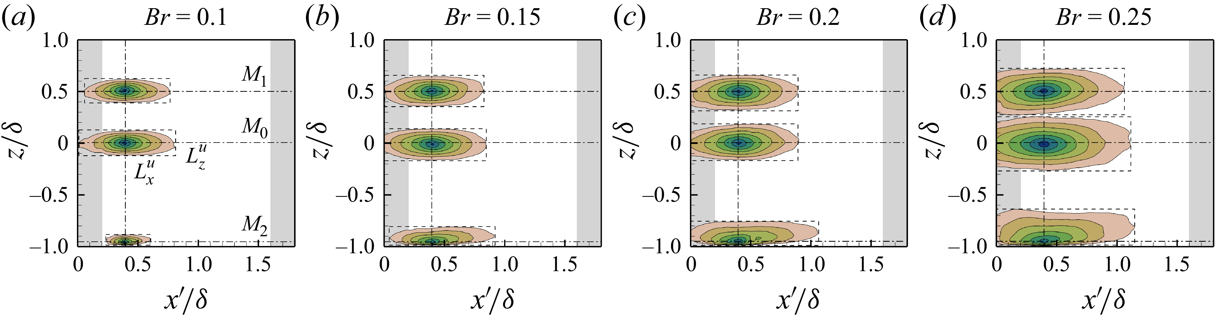


 Open access