


1. Introduction
The study of passive scalars evolving in wall turbulence is of great practical significance. For example, it is representative of the diffusion of pollutants, and the evolution of the temperature field in low-Mach-number flows with small temperature differences (Cebeci & Bradshaw Reference Cebeci and Bradshaw2012; Lim & Vanderwel Reference Lim and Vanderwel2023). As accurate measurements of statistics of the passive tracers are quite challenging (Gowen & Smith Reference Gowen and Smith1967; Kader Reference Kader1981; Nagano & Tagawa Reference Nagano and Tagawa1988), direct numerical simulation (DNS) has become an excellent tool for investigating the passive scalar in wall-bounded turbulence, which can provide ample information related to the details of the passive scalar field. A growing body of knowledge about the physical characteristics of the passive scalar has been accumulated due to enhanced computing power.
As early as the 1980s, Kim & Moin (Reference Kim and Moin1989) firstly performed the DNSs of passive scalars in incompressible turbulent channel flows at  $Re_{\tau }=180$ ( $Re_{\tau }=u_{\tau }h/\nu _{w}$ denotes the friction Reynolds number; $u_{\tau }$ is the friction velocity, $\nu _{w}$ the kinematic viscosity at the wall and $h$ the channel half-width; the subscript $w$ refers to the quantities evaluated at the wall surface) with various molecular Prandtl numbers $Pr$ by adding a uniform volumetric body force into the passive scalar transport equation. Subsequently, Kawamura, Abe & Matsuo (Reference Kawamura, Abe and Matsuo1999) and Abe, Kawamura & Matsuo (Reference Abe, Kawamura and Matsuo2004) further extended the Reynolds number of the simulation to achieve a discernible scale separation. All these pioneer works reported the similarities between the passive scalar and streamwise velocity fields in the near-wall region when $Pr$ is close to unity, which conform to the celebrated Reynolds analogy (Kader Reference Kader1981). Specifically, the passive scalar is observed to organize in a streaky manner, which resembles the low- and high-speed velocity streaks in the vicinity of the wall. The length scales of these streaky scalars are found to be scaled in viscous units. High-Reynolds-number simulations have been achieved in the last decade. Pirozzoli, Bernardini & Orlandi (Reference Pirozzoli, Bernardini and Orlandi2016) and Alcántara-Ávila, Hoyas & Pérez-Quiles (Reference Alcántara-Ávila, Hoyas and Pérez-Quiles2021) simulated the incompressible channel flows with passive scalars at $Pr\leq 1$ when $Re_{\tau }\approx 4000$ and $Re_{\tau }\approx 5000$, respectively. Very recently, Pirozzoli et al. (Reference Pirozzoli, Romero, Fatica, Verzicco and Orlandi2022) conducted a simulation of pipe flow at $Re_{\tau }\approx 6000$, including a passive scalar field with $Pr=1$. With the accumulation of the DNS database, some differences between the passive scalar and streamwise velocity fields have been uncovered. Based on the dataset built in a previous study (Abe et al. Reference Abe, Kawamura and Matsuo2004), Abe & Antonia (Reference Abe and Antonia2009) reported that flawed similarities can be traced in the regions where the streamwise pressure gradient is large due to the existence of near-wall vortices. Pirozzoli et al. (Reference Pirozzoli, Bernardini and Orlandi2016) also observed that the interfaces between the adjacent motions of the scalar field are sharper than those of the velocity fields. It is worth noting that these results are all qualitative, and other analytical approaches should be developed to quantify these differences. This is one of the objectives of the present study.
For the high-fidelity simulation of the passive scalar in compressible wall-bounded turbulence, however, the existing works are quite scarce. This is mainly due to the huge computational resources required to solve the compressible Navier–Stokes (NS) equations along with a passive scalar transport equation. Friedrich, Foysi & Sesterhenn (Reference Friedrich, Foysi and Sesterhenn2006) performed a series of DNSs of compressible turbulent channel flows, including passive scalar transport with Mach numbers ranging from 0.3 to 3.5. The passive scalar is added to the flow through one channel wall and removed through the other. However, the semilocal friction Reynolds numbers  $Re_{\tau }^*$ of their cases are not high ( $R e_{\tau }^{*}=R e_{\tau } \sqrt {(\bar {\rho }_c / \bar {\rho }_{w})} /(\bar {\mu }_c / \bar {\mu }_{w})$; $\rho$ is the density, $\mu$ the dynamic viscosity; the subscript $c$ refers to the quantities evaluated at the channel centre; $\bar {\cdot }$ denotes the average value). We take special care of the $Re_{\tau }^*$ of the simulations because previous studies indicate that $Re_{\tau }^{*}$ can reasonably clarify the Reynolds-number effects on the statistics involving the thermodynamic and the velocity variables in compressible channel flows (Gerolymos & Vallet Reference Gerolymos and Vallet2014; Patel et al. Reference Patel, Peeters, Boersma and Pecnik2015; Griffin, Fu & Moin Reference Griffin, Fu and Moin2021; Huang, Duan & Choudhari Reference Huang, Duan and Choudhari2022; Cheng et al. Reference Cheng, Chen, Zhu, Shyy and Fu2024). The magnitude of $Re_{\tau }^*$ should be high enough to obtain a discernible logarithmic region, which is a primary condition for investigating the multiscale eddies and their interactions in depth.
In our previous work (Cheng & Fu Reference Cheng and Fu2023a), we resorted to the spectral linear stochastic estimation (SLSE) to dissect the coupling between the velocity and temperature fields in compressible channel flows. It has been demonstrated that this coupling is tight at the scales corresponding to the energy-containing motions in the wall-normal position under consideration, such as the self-similar attached eddies in the logarithmic region (Townsend Reference Townsend1976), and the very large-scale motions (VLSMs) in the outer region (Hutchins & Marusic Reference Hutchins and Marusic2007). One of the referees posed a profound question concerning this result, that is, how much of this observed coupling can be attributed to a genuine dynamical interaction between the energy and momentum equations, and how much is a simple transport effect? The equivalent question is: to what extent can the temperature field in compressible wall turbulence be considered as a passive scalar? A derivative question is in which part of the boundary layer do the features of the temperature field depart from those of a passive scalar field most? It is undeniable that a wide variety of previous studies have reported the similarities between the streamwise velocity and temperature fields in compressible wall-bounded turbulence, for example Cheng & Fu (Reference Cheng and Fu2022b) and Chen et al. (Reference Chen, Cheng, Fu and Gan2023a,Reference Chen, Cheng, Gan and Fub), to name a few. However, these existing works cannot measure the degree of similarity between the temperature, streamwise velocity and passive scalar fields. In light of this, there is no doubt that performing DNSs of compressible wall turbulence with passive scalars at moderate Reynolds number and appraising the multiphysics couplings by appealing to the SLSE is a cogent approach to elucidate the proposed problems. It also helps to address the lack of statistics on the passive scalar in compressible wall turbulence in the literature.
In the present study, we are thus dedicated to the multiphysics couplings in the subsonic/supersonic turbulent channel flows, which are comprised of the velocity–temperature ( $u-T$), scalar–temperature ( $g-T$) and velocity–scalar ( $u-g$) couplings. We first elaborate on clarifying the differences between the streamwise velocity and the passive scalar. Through the lens of governing equations, the underlying mechanisms of these differences can be attributed to two factors: one is the distinct form of the viscous terms in the streamwise momentum equation and the passive scalar transport equation (for incompressible flows, their forms are identical); another is the inclusion of the pressure field in the streamwise momentum equation of the NS equations, instead of the passive scalar transport equation. Hence, we will analyse their effects separately by conducting well-designed DNSs and employing the SLSE as the diagnostic tool. Based on these novel understandings, we will then concentrate on the role of the temperature in the flow field, i.e. to what extent can the temperature be treated as a passive scalar? Moreover, we will also focus on the connection between the multiphysics couplings and the pressure field.
The remainder of this paper is organized as follows. In §§ 2 and 3, the designed DNS cases and the SLSE approach are introduced, respectively. The effects of the different forms of the viscous terms and the inclusion of the pressure field on the multiphysics couplings are investigated in §§ 4 and 5, separately. In § 6, some discussions are given, such as the relationship between the temperature and passive scalar fields, the relationship between the pressure and velocity fields, and the Reynolds-number and Mach-number effects on the multiphysics couplings. Concluding remarks are present in § 7.
2. Numerical simulation set-ups
We conduct numerical simulations of supersonic channel flows at a series of Mach numbers  $M_b=U_b/C_w$ ( $U_b$ is the bulk velocity, and $C_w$ is the speed of sound at wall temperature) and Reynolds numbers $Re_b=\rho _bU_bh/\mu _w$. All these cases are performed in a computational domain of $4{\rm \pi} h\times 2{\rm \pi} h\times 2 h$ in the streamwise ( $x$), spanwise ( $z$) and wall-normal ( $\kern 1.5pt y$) directions, respectively. Numerous previous studies have verified that these set-ups of dimensions can resolve most of the energy-containing motions in the logarithmic and outer regions of a boundary layer (Agostini & Leschziner Reference Agostini and Leschziner2014; Cheng & Fu Reference Cheng and Fu2023a). Both the Reynolds (denoted as $\bar {\phi }$) and the Favre averaged (denoted as $\tilde {\phi }=\overline {\rho \phi }/\bar {\rho }$) statistics are used in the present study. The corresponding fluctuating components are represented as $\phi '$ and $\phi ''$, respectively.
The simulations have been conducted with a finite-difference code, by mainly solving the non-dimensional three-dimensional compressible NS equations along with a standard passive scalar transport equation (not the single transport equation solved in the present study), which take the form of
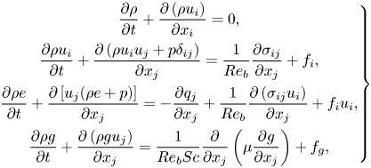 \begin{equation} \left.\begin{gathered} \frac{\partial \rho}{\partial t}+\frac{\partial\left(\rho u_i\right)}{\partial x_i}=0, \\ \frac{\partial \rho u_i}{\partial t}+\frac{\partial\left(\rho u_i u_j+p \delta_{i j}\right)}{\partial x_j}=\frac{1}{R e_b} \frac{\partial \sigma_{i j}}{\partial x_j}+f_i, \\ \frac{\partial \rho e}{\partial t}+\frac{\partial\left[u_j(\rho e+p)\right]}{\partial x_j}={-}\frac{\partial q_j}{\partial x_j}+\frac{1}{R e_b} \frac{\partial\left(\sigma_{i j} u_i\right)}{\partial x_j}+f_iu_i, \\ \frac{\partial \rho g}{\partial t}+\frac{\partial\left(\rho g u_j\right)}{\partial x_j}=\frac{1}{R e_bSc} \frac{\partial } {\partial x_j}\left(\mu \frac{\partial g}{\partial x_j}\right)+f_g, \end{gathered}\right\} \end{equation}
where  $u_i$, $p$,
$p$,  $q_j$, $g$ and $\sigma _{i j}$ denote the velocity component, the pressure, the components of the heat-flux vector, the scalar and the viscous stress tensor, respectively. Here $e=c_vT+u_iu_i/2$ is the total energy per unit mass, where $T$ and $c_v$ denote the temperature and the specific heat at constant volume, respectively. The heat flux $q_j$ is calculated through Fourier's law, i.e. $q_j=-k\partial T/\partial x_j$, where $k=c_p\mu /Pr$ with $c_p$ being the specific heat at constant pressure and $Pr=0.72$. The Kronecker symbol is $\delta _{i j}$. For the scalar transport equation, $Sc$ represents the Schmidt number. In the present study, $u$,
$u$,  $w$ and $v$ denote the velocities along the streamwise ( $x$), spanwise ( $z$) and wall-normal ( $\kern 1.5pt y$) directions, respectively, and a specific heat ratio $\gamma$ of 1.4 is employed with $c_v=1/(M_b^2\gamma (\gamma -1))$ and $c_p=\gamma c_v$.
The convective terms are discretized with a seventh-order upwind-biased scheme, and the viscous terms are evaluated with an eighth-order central difference scheme. Time advancement is performed using the third-order strong-stability-preserving Runge–Kutta method (Gottlieb, Shu & Tadmor Reference Gottlieb, Shu and Tadmor2001). The dependence of dynamic viscosity  $\mu$ on temperature $T$ is given by Sutherland's law, i.e.
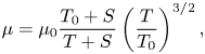 \begin{equation} \mu=\mu_{0} \frac{T_{0}+S}{T+S}\left(\frac{T}{T_{0}}\right)^{3 / 2}, \end{equation}
where  $S=110.4\ \textrm {K}$ and $T_0=273.1\ \textrm {K}$. The fluid is Newtonian with the viscous shear stress modelled as
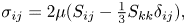 \begin{equation} \sigma_{i j}=2 \mu(S_{i j}-\tfrac{1}{3} S_{k k} \delta_{i j}), \end{equation}
where  $S_{i j}=(\partial u_i / \partial x_j+\partial u_j / \partial x_i) / 2$ is the rate of the strain tensor.
The isothermal no-slip conditions are imposed at the top and bottom walls, and the periodic boundary condition is imposed in the wall-parallel directions, i.e. the  $x$ and $z$ directions. For the scalar field, $g$ is set as zero at the walls. All simulations begin with a fully developed field of similar parameter set-up obtained in our previous studies (Cheng & Fu Reference Cheng and Fu2022b, Reference Cheng and Fu2023a; Bai, Cheng & Fu Reference Bai, Cheng and Fu2023a; Bai et al. Reference Bai, Cheng, Griffin, Li and Fu2023b; Cheng, Shyy & Fu Reference Cheng, Shyy and Fu2023) (see tables 1 and 2 of the current study). The initial scalar field is copied from the instantaneous streamwise velocity field at this instant. A body force $f_i$ is imposed in the streamwise direction to maintain a constant mass flow rate, and a corresponding source term $f_iu_i$ is also added to the energy equation. For the passive scalar, $f_g$ in (2.1) is also used to keep the flow rate of $\rho g$ to be constant (similar to the body force added to the streamwise momentum equation). It represents a circumstance where the passive scalar is created internally and removed from both walls. In other words, the boundary and initial conditions are identical for $u$ and $g$. Similar set-ups were also built by Pirozzoli et al. (Reference Pirozzoli, Bernardini and Orlandi2016) to simulate the incompressible channel flows with passive scalars. The validation of the code is provided in Appendix A.
Table 1. Parameter settings of the first type compressible DNS database (D1) by solving the NS equations with (2.4). Here,  $N_x$, $N_y$, $N_z$ denote numbers of computational grid points in streamwise, wall-normal and spanwise directions, respectively, and $\Delta x^+$ and $\Delta z^+$ denote the streamwise and spanwise grid resolutions in viscous units, respectively. Here $\Delta y_{min}^+$ and $\Delta y_{max}^+$ denote the finest and the coarsest resolution in the wall-normal direction, respectively, and $Tu_{\tau }/h$ indicates the total eddy turnover time used to accumulate statistics.
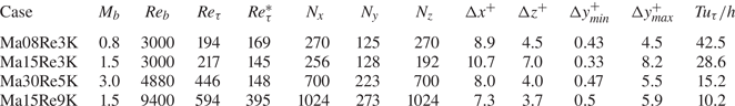
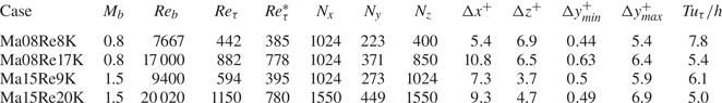
Table 2. Parameter settings of the second type compressible DNS database (D2) by solving (2.1).
In the present study,  $Sc$ is fixed at unity. This treatment ensures that the scalar transport equation in (2.1) resembles the streamwise momentum equation to the utmost extent. Under this condition, the $u-g$ coupling is the tightest without doubt, and the major factors that contribute to the differences between $u$ and $g$ fields can be isolated. They can be divided into two types from the prism of the governing equations. The first one is the pressure-term-related factor (PRF), which manifests as the involvement of the pressure field in the streamwise momentum equation, but not in the standard scalar transport equation. In this case, different from $g'$,
$g'$,  $u'$ is not passively advected, and it can react to the formation of the fronts by feedback pressure (Pirozzoli et al. Reference Pirozzoli, Bernardini and Orlandi2016). The PRF also exists in incompressible flows (Kim & Moin Reference Kim and Moin1989; Abe & Antonia Reference Abe and Antonia2009), though it is not as complicated as in compressible ones due to the absence of the energy governing equation. The second is the viscous-term-related factor (VRF), which shows that the velocity and scalar gradients are involved in the momentum and scalar transport equations in distinct styles. For compressible wall turbulence, the compressibility plays a non-negligible role in the VRF, which is manifested as the inclusion of the expansion term $\boldsymbol {\triangledown } \boldsymbol {\cdot } \boldsymbol {u}$ in $\sigma _{i j}$. Additionally, the dynamic viscosity $\mu$ is temperature-dependent, which can also influence the magnitude of $\sigma _{i j}$. This intricate scenario does not exist for incompressible wall turbulence. The VRF can be studied in depth by comparing the $u$ and $g$ fields in specially established cases via solving an off-standard scalar transport equation along with the standard NS equations, namely,
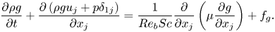 \begin{equation} \frac{\partial \rho g}{\partial t}+\frac{\partial\left(\rho g u_j+p \delta_{1 j}\right)}{\partial x_j}=\frac{1}{R e_bSc} \frac{\partial }{\partial x_j}\left(\mu \frac{\partial g}{\partial x_j}\right)+f_g. \end{equation}
In this way, the scalar also becomes active like the streamwise velocity, and the main differences between these two fields should be ascribed to the VRF, rather than the PRF. Small differences between the momentum and passive scalar equations may originate from the nonlinearity in the momentum equation. As we will see in § 4.2, it exerts negligible effects on the multiphysics couplings.
Based on the above analyses, the simulations conducted in the present study are well-designed. First, the VRF is dissected alone by solving (2.4) along with the NS equations. Details of the parameter settings of the formed database are listed in table 1. This type of data is named D1 herein and can be considered as a kind of numerical experiment. After all, this type of scalar field does not exist in reality. The cases Ma08Re3K, Ma15Re3K and Ma30Re50K in D1 are employed to examine the Mach-number effects. The semilocal friction Reynolds numbers of these cases are nearly identical to varying Mach numbers. The cases Ma15Re3K and Ma15Re9K are used to investigate the Reynolds-number effects. We will show in § 4 that the VRF takes effect in the near-wall region only. Second, the PRF is studied by solving (2.1). Our analyses in the following contents reveal that the PRF is dominant in the logarithmic and outer regions. The enlargement of the simulated  $Re_b$ is beneficial for obtaining a discernible logarithmic region for the facilitation of investigation. Details of the parameter settings of this type of database are listed in table 2, and named as D2. The maximum number of grid points is in excess of $1\times 10^{9}$. The cases Ma08Re17K and Ma15Re20K with the highest $Re_{\tau }^{*}$ are mainly used to show the results in following sections. The cases Ma08Re8K and Ma08Re17K are of similar $Re_{\tau }^{*}$ with those of Ma15Re9K and Ma15Re20K, which are adopted in § 6.4 to clarify the Mach-number and Reynolds-number effects. As a side note, the ratio between the Batchelor scalar dissipative scale ( $\eta _g$) and the Kolmogorov scale ( $\eta$) is approximately $Sc^{-0.5}$ (Batchelor Reference Batchelor1959). As $Sc$ is maintained as unity in the present study, $\eta _g$ approaches $\eta$. Hence, the grid resolutions of these cases are sufficient for capturing the typical structures of the scalar field. In Appendix B, the effects of the grid resolution on the statistical properties of passive scalar and the related multiphysics couplings are investigated. It is demonstrated that the grid resolutions listed in table 2 are sufficient for resolving them when $Sc=1$.
Throughout the study, we use the superscript  $+$ to represent the normalization with $\rho _w$, the friction velocity $u_{\tau }$, the friction temperature (denoted as $T_{\tau }$, $T_{\tau }=q_{w}/\rho _w c_p u_\tau$, $q_{w}$ is the mean heat flux on the wall), the viscous length scale (denoted as $\delta _{\nu }$, $\delta _{\nu }=\nu _w/u_{\tau }$, $\nu _w=\mu _w/\rho _w$) and the friction scalar $g_{\tau }$, which is defined as (Friedrich et al. Reference Friedrich, Foysi and Sesterhenn2006)
 \begin{equation} g_{\tau}=\left.\left.\overline{\frac{\mu}{Sc} \frac{\partial g}{\partial y}}\right|_{w}\right/(\rho_wu_\tau). \end{equation}
We also use the superscript  $*$ to represent the normalization with the semilocal wall units, i.e. $u_{\tau }^*=\sqrt {\tau _w/\bar {\rho }}$ and $\delta _{\nu }^*=\overline {\nu (y)}/u_{\tau }^*$.
3. Diagnostic tool: spectral linear stochastic estimation and correlation function
In our previous study, we introduced the SLSE to dissect the coupling between the velocity and temperature fields in compressible wall turbulence and also demonstrated its effectiveness (Cheng & Fu Reference Cheng and Fu2023a). In the present study, we extend it to study the multiphysics interactions associated with the  $u$,
$u$,  $g$ and $T$ fields here. The SLSE employed in the present study can be divided into two branches, and are briefly introduced here in return.
The DNS instantaneous fields at a given wall-normal height can be decomposed into Fourier coefficients along the streamwise and spanwise directions by leveraging the homogeneity along these two directions. The SLSE fully takes advantage of this. The comparison between the  $u-T$ and $g-T$ couplings can shed light on the differences between velocity and passive scalar fields resulting from the PRF and VRF. Because if they do not exist, $u-T$ and $g-T$ couplings must be totally identical in the spectral domain. Hence, the first branch of SLSE takes the form of
 \begin{equation} T_{p}^{\prime}\left(y\right)=F_{x,z}^{{-}1}\left\{H_{\varPhi T}\left(\lambda_{x},\lambda_{z}; y\right) F_{x,z}\left[\varPhi^{\prime}\left(y\right)\right]\right\}, \end{equation}
where  $T_{p}^{\prime }$ denotes the predicted value of the variable $T'$, and $\varPhi$ can be $u$ or $g$. Here $F_{x,z}$ and $F_{x,z}^{-1}$ denote the two-dimensional (2-D) fast Fourier transform and the inverse 2-D fast Fourier transform in the streamwise and the spanwise directions, respectively. Here $H_{\varPhi T}$ is the transfer kernel, which evaluates the correlation between $\widehat {T_{}^{\prime }}(y)$ and $\widehat {\varPhi '}(y)$ at streamwise length scale $\lambda _{x}$ and spanwise length scale $\lambda _{z}$, and can be calculated as
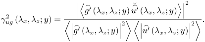
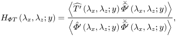 \begin{equation} H_{\varPhi T}\left(\lambda_{x},\lambda_{z};y\right)=\frac{\left\langle\widehat{T'}\left(\lambda_{x},\lambda_{z}; y\right) \breve{\widehat{\varPhi'}}\left(\lambda_{x},\lambda_{z}; y_{}\right)\right\rangle}{\left\langle\hat{\varPhi'}\left(\lambda_{x},\lambda_{z}; y\right) \breve{\widehat{\varPhi'}}\left(\lambda_{x},\lambda_{z}; y\right)\right\rangle}, \end{equation}
where  $\langle \cdot \rangle$ denotes the ensemble averaging, $\widehat {\varPhi '}$ and $\widehat {T^{\prime }}$ are the Fourier coefficients of $\varPhi '$ and $T'$, respectively, and $\breve {\widehat {\varPhi ^{\prime }}}$ represents the complex conjugate of $\widehat {\varPhi ^{\prime }}$. In some sense, $T_{p}^{\prime }(y)$ in (3.1) is the component of $T'(y)$ that is linearly correlated with the $\varPhi '(y)$ at a given wall-normal height $y$. In Cheng & Fu (Reference Cheng and Fu2023a), we utilized the density-weighted streamwise velocity fluctuation ( $\sqrt {\rho }u^{\prime \prime }$) as the input signal $\varPhi '$ in (3.1). As we have observed that the results of the employment of $u^{\prime }$ are nearly identical with those of $\sqrt {\rho }u^{\prime \prime }$, we use $u'$ in the present study for the sake of conciseness. To further measure the coherence between $T^{\prime }(y)$ and $\varPhi '(y)$, a 2-D linear coherence spectrum (LCS) is also introduced here by following previous studies (Baars, Hutchins & Marusic Reference Baars, Hutchins and Marusic2017; Baars & Marusic Reference Baars and Marusic2020; Cheng & Fu Reference Cheng and Fu2022a), and can be cast as
 \begin{equation} \gamma^2_{\varPhi T}\left(\lambda_{x},\lambda_{z};y\right)=\frac{\left|\left\langle\widehat{T'}\left(\lambda_{x},\lambda_{z}; y\right) \breve{\widehat{\varPhi^{\prime}}}\left(\lambda_{x},\lambda_{z}; y_{}\right)\right\rangle\right|^2}{\left\langle\left|\widehat{T'}\left(\lambda_{x},\lambda_{z}; y\right)\right|^2\right\rangle\left\langle\left|\widehat{\varPhi'}\left(\lambda_{x},\lambda_{z}; y\right)\right|^2\right\rangle}, \end{equation}
where  $|\cdot |$ is the modulus. Here $\gamma ^{2}_{\varPhi T}$ evaluates the square of the scale-specific correlation between $\varPhi '(y)$ and $T^{'}(y)$ with $0\leq \gamma ^{2}_{\varPhi T}\leq 1$ (Bendat & Piersol Reference Bendat and Piersol2011). Here $\gamma ^{2}_{\varPhi T}=1$ indicates a perfectly linear correlation between the $T'$ and $\varPhi '$ signals at a wavelength pair ( $\lambda _{x}$, $\lambda _{z}$), whereas $\gamma ^{2}_{\varPhi T}=0$ implies a purely uncorrelated relationship. Moreover, the overall intensity of $\varPhi -T$ coupling can be further quantified by calculating the relative deviation (RD), which reads as
 \begin{equation} RD_{\varPhi T}=\frac{\overline{T^{\prime 2}}-\overline{T_p^{\prime 2}}}{\overline{T^{\prime 2}}}. \end{equation}
The smaller  $RD_{\varPhi T}$, the tighter $\varPhi -T$ coupling, and vice versa.
Another branch of SLSE aims to inspect the  $u-g$ coupling directly, namely,
 \begin{equation} g_{p}^{\prime}\left(y\right)=F_{x,z}^{{-}1}\left\{H_{ug}\left(\lambda_{x},\lambda_{z}; y\right) F_{x,z}\left[u^{\prime}\left(y\right)\right]\right\}. \end{equation}
Similarly, the kernel function  $H_{ug}$ can be expressed as
 \begin{equation} H_{ug}\left(\lambda_{x},\lambda_{z};y\right)=\frac{\left\langle\widehat{g'}\left(\lambda_{x},\lambda_{z}; y\right) \breve{\widehat{u'}}\left(\lambda_{x},\lambda_{z}; y\right)\right\rangle}{\left\langle\widehat{u'}\left(\lambda_{x},\lambda_{z}; y\right) \breve{\widehat{u'}}\left(\lambda_{x},\lambda_{z}; y\right)\right\rangle}. \end{equation}
The related LCS reads as
 \begin{equation} \gamma^2_{ug}\left(\lambda_{x},\lambda_{z};y\right)=\frac{\left|\left\langle\widehat{g'}\left(\lambda_{x},\lambda_{z}; y\right) \breve{\widehat{u^{\prime}}}\left(\lambda_{x},\lambda_{z}; y_{}\right)\right\rangle\right|^2}{\left\langle\left|\widehat{g'}\left(\lambda_{x},\lambda_{z}; y\right)\right|^2\right\rangle\left\langle\left|\widehat{u'}\left(\lambda_{x},\lambda_{z}; y\right)\right|^2\right\rangle}. \end{equation}
Finally, the corresponding relative deviation can also be defined as
 \begin{equation} RD_{ug}=\frac{\overline{g^{\prime 2}}-\overline{g_p^{\prime 2}}}{\overline{g^{\prime 2}}}. \end{equation}
 As can be seen,  $T'$ in the first branch of SLSE serves as a bridge between the $u'$ and $g'$ fields. This treatment is not arbitrary. On the one hand, $T'$ is typically considered as a passive scalar in incompressible wall turbulence (Abe & Antonia Reference Abe and Antonia2009; Antonia, Abe & Kawamura Reference Antonia, Abe and Kawamura2009) and compressible wall turbulence at low Mach number (Chen et al. Reference Chen, Cheng, Fu and Gan2023a; Cheng & Fu Reference Cheng and Fu2023b), just like $g'$. On the other hand, $T'$ can strikingly influence the $u'$ field through the interactions between the momentum and energy equations in compressible wall turbulence, whereas $g'$ cannot. Hence, the $T'$ field is highly linked with both $u'$ and $g'$ concurrently, and thus choosing it as the connection is logical. Moreover, investigating the PRF and the VRF from the prism of the $u-T$ and $g-T$ couplings can reveal a wealth of information about the multiphysics interactions in compressible wall turbulence.
At last, we briefly introduce another classical method adopted in the present study to cast light on the multiphysics couplings, namely, the correlation function. For a variable  $\varPhi$ (similarly, $\varPhi$ can be $u$ or $g$), its correlation with $T'$ can be defined as
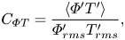 \begin{equation} C_{\varPhi T}=\frac{\left\langle \varPhi^{\prime} T^{\prime}\right\rangle}{\varPhi_{rms}^{\prime} T_{rms}'}, \end{equation}
where the subscript ‘rms’ denotes the root-mean-square (r.m.s.) of the corresponding variable. The larger  $C_{\varPhi T}$, the tighter $\varPhi -T$ coupling, and vice versa. Compared with $RD_{\varPhi T}$ defined in (3.4), the correlation function $C_{\varPhi T}$ is a more direct metric to measure the degree of the $\varPhi -T$ coupling as a whole. Similarly, the function $C_{ug}$ reads as
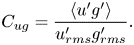 \begin{equation} C_{ug}=\frac{\left\langle u^{\prime} g^{\prime}\right\rangle}{u_{rms}^{\prime} g_{rms}'}. \end{equation}
In the next sections, we will deploy these tools introduced here to clarify the multiphysics couplings.
4. Effects of the VRF
The major differences between the  $u$ and $g$ fields can be ascribed to the emergence of the VRF and the PRF. The cooperation of the pressure field in the convective term of the non-standard scalar transport equation (namely, (2.4)) would make the scalar be active, and aid in isolating the effects of the VRF. The formed DNS database D1 is analysed in the present section, and we pay extensive attention to the differences between the $u'$ and $g'$ fields and their couplings with the third-party variable $T'$.
$T'$.
4.1. General turbulence statistics
In this subsection, we are dedicated to dissecting the effects of VRF on the general turbulence statistics. These analyses can give us an overview of the effects originating from VRF. Figure 1(a,b) compares the viscous-scaled mean (figure 1a) and second-order ( $\overline {\varPhi ^{\prime 2}}^+$) statistics (figure 1b) for the cases in D1 with different Mach numbers but similar $Re_{\tau }^*$, i.e. Ma08Re3K, Ma15Re3K and Ma30Re5K. It is noted that the magnitudes of $u_{\tau }$ and $g_{\tau }$ are very close to each other. Both the mean and second-order profiles of the cases with larger $M_b$ are up-shifted. At a fixed $M_b$, the profiles of $u$ and $g$ overlap with each other. It suggests that the VRF cannot lead to the disparity of the low-order statistics related to the two fields. However, when high-order moments are taken into account, the differences emerge. Figure 1(c,d) shows the corresponding profiles of the skewness ( $S_{\varPhi }$) (figure 1c) and the flatness (figure 1d) ( $F_{\varPhi }$), respectively. It can be seen that $S_{g}$ and $F_{g}$ are remarkably smaller than those of $u'$ in the near-wall region ( $\kern 1.5pt y^*<20$) at a given $M_b$. It indicates that the $u'$ field is more intermittent than the $g'$ field due to the occurrence of VRF. This scenario is significant in the near-wall region, where the viscous effects and the compressibility are the strongest (Coleman, Kim & Moser Reference Coleman, Kim and Moser1995). Moreover, the differences between the high-order moments of $u'$ and $g'$ are more obvious for a larger $M_b$. It indicates that the VRF leads to the distinct frequencies of occurrence of the extreme events for $u'$ and $g'$ in the vicinity of the wall more or less. We have also checked the instantaneous fields and the spectra of these two variables at a given $y^*$. Both $u'$ and $g'$ bear streaky shapes in the near-wall region, just like the patterns in incompressible flows (Abe et al. Reference Abe, Kawamura and Matsuo2004; Abe & Antonia Reference Abe and Antonia2009), and no visible difference can be found. We do not show them here for the sake of brevity.

Figure 1. Variations of ( $a$) the viscous-scaled mean statistics, ( $b$) the second-order statistics, ( $c$) the skewness and ( $d$) the flatness of $u'$ and $g'$ as functions of $y^*$ for the cases in D1 with different Mach numbers. All cases are of $Re_{\tau }^{*}\approx 150$.
Next, we pay attention to the VRF effects in cases with different Reynolds numbers. Figure 2(a,b) shows the variations of the skewness (figure 2a), and the flatness (figure 2b) as functions of  $y^*$ for the cases Ma15Re3K and Ma15Re9K in D1. The two cases are of identical Mach numbers but different Reynolds numbers. It is not difficult to observe that for both cases, the distributions of the high-order statistics of $u'$ and $g'$ only show differences below $y^*<100$. It signifies that the effects of VRF are restricted to the near-wall region. This is expected because in the logarithmic and outer regions, the influences originating from the molecular viscosity are negligible (Pope Reference Pope2000), so are the viscous terms in (2.1) and (2.4).
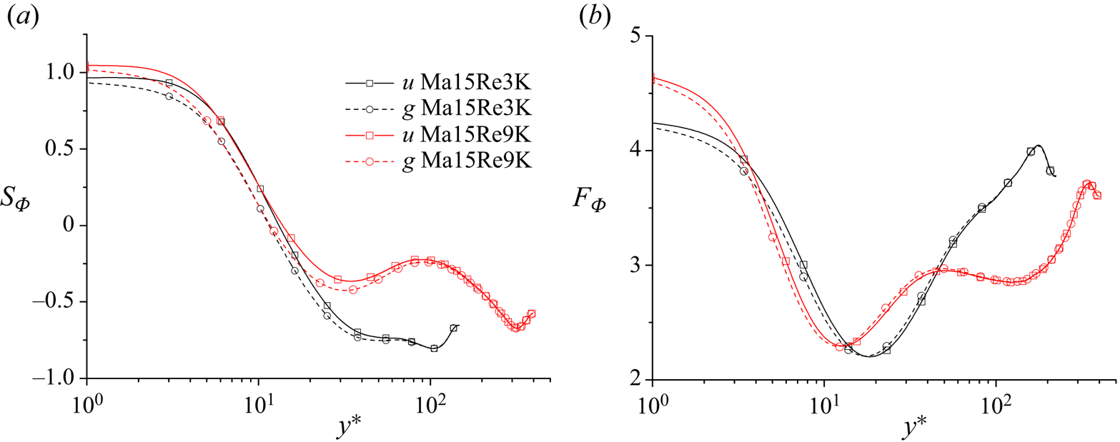
Figure 2. Variations of ( $a$) the skewness, and ( $b$) the flatness of $u'$ and $g'$ as functions of $y^*$ for the cases Ma15Re3K and Ma15Re9K in D1.
All in all, the VRF mainly affects the intermittency of  $u'$ and $g'$ in the near-wall region ( $\kern 1.5pt y^*<100$), and the enlargement of the Mach number enhances this difference.
4.2. Multiphysics couplings
The subtle modification of the intermittency by the VRF might affect the multiphysics couplings in the vicinity of the wall. In this subsection, we will resort to the diagnostic tool introduced in § 3, namely the SLSE, to shed light on this effect.
Let us examine the variations of  $RD_{uT}$ and $RD_{gT}$ first, which are helpful for the reader to have an overview of the $u-T$ and $g-T$ couplings. Figure 3(a) shows the variations of $RD_{\varPhi T}$ as functions of $y^*$ for cases in D1 with $Re_{\tau }^{*}\approx 150$ but different Mach numbers. The linear model can recover over $95\,\%$ of $\overline {T^{\prime 2}}$ for both $u$ and $g$ below $y^*=10$. This relative error, however, rapidly increases as the wall-normal height increases. As expected, the profiles of $RD_{u T}$ and $RD_{g T}$ collapse with each other above the near-wall region in each case, regardless of the Mach number. It suggests that the VRF can only affect the $u-T$ and $g-T$ couplings in the vicinity of the wall. A similar scenario can be observed in the cases with $M_b=1.5$ but different Reynolds numbers, whose results are displayed in figure 3(b). Interestingly, the $RD_{g T}$ of a case is slightly larger than $RD_{u T}$ in the vicinity of the wall. Figure 3(c,d) shows the same results, but as functions of $y/h$. It can be seen that only the profiles with similar $Re_{\tau }^{*}$ collapse well beyond the near-wall region. Figure 3(e,f) shows the counterparts for $u-g$ coupling. The maximum value of $RD_{u g}$ is less than $3\,\%$ along the whole boundary layer, regardless of the Mach and Reynolds numbers. These results suggest that $u-g$ couplings in these cases are rather robust. We also inspect the LCSs related to the $u-T$ and $u-g$ couplings at a given wall-normal height. No evident difference can be found. It indicates that the VRF cannot alter the scale-based correlations among $u-T$ and $g-T$.

Figure 3. (a,b) Variations of  $RD_{\varPhi T}$ as functions of $y^*$ for (a) the cases with $Re_{\tau }^{*}\approx 150$ but different Mach numbers, and (b) the cases with $M_b=1.5$ but different Reynolds numbers; (c,d) variations of $RD_{\varPhi T}$ as functions of $y/h$ for (c) the cases with $Re_{\tau }^{*}\approx 150$ but different Mach numbers, and (d) the cases with $M_b=1.5$ but different Reynolds numbers; (e,f) variations of $RD_{u g}$ as functions of $y^*$ for (e) the cases with $Re_{\tau }^{*}\approx 150$ but different Mach numbers, and (f) the cases with $M_b=1.5$ but different Reynolds numbers.
Next, figure 4 reports the corresponding results with regard to the correlation functions. It is not difficult to observe that they are highly consistent with those of the SLSE. Combining the observations in figures 3 and 4, we can conclude that changing the Reynolds number has more remarkable effects on the degree of the  $u-T$ and $g-T$ couplings than the Mach number beyond the near-wall region. In § 5, our analyses suggest that $u-T$ coupling at a given wall-normal position is highly linked with the energy-containing motions populating this region. The enlargement of the Reynolds number would result in a more significant scale separation and thus intensifying the $u-T$ coupling. The changing of the Mach number cannot bring about such an effect, at least within the cases under investigation. Furthermore, $C_{ug}\approx 1$ is maintained in all cases, regardless of the Reynolds and Mach numbers, see figure 4(e,f), which demonstrates again that the VRF bears little effect on the $u-g$ coupling. In Appendix C, we compare the variation tendencies of $1-RD_{\varPhi T}$ and $C_{\varPhi T}$ by plotting them together. It can help the readers to have an overview of the consistency between these two quantities.
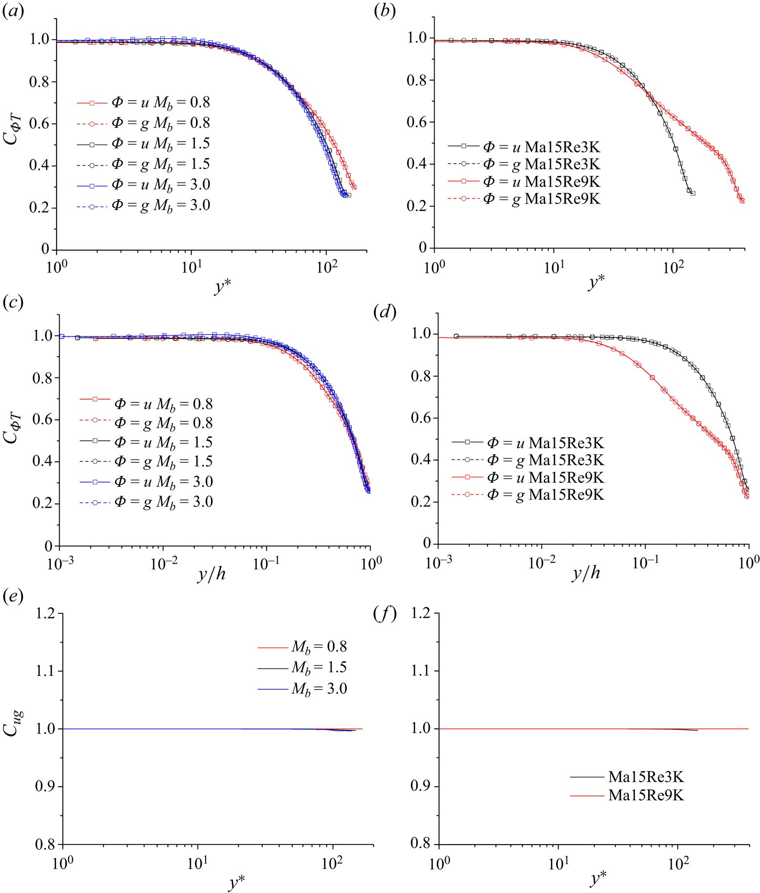
Figure 4. (a,b) Variations of  $C_{\varPhi T}$ as functions of $y^*$ for (a) the cases with $Re_{\tau }^{*}\approx 150$ but different Mach numbers, and (b) the cases with $M_b=1.5$ but different Reynolds numbers; (c,d) variations of $C_{\varPhi T}$ as functions of $y/h$ for (c) the cases with $Re_{\tau }^{*}\approx 150$ but different Mach numbers, and (d) the cases with $M_b=1.5$ but different Reynolds numbers; (e,f) variations of $C_{u g}$ as functions of $y^*$ for (e) the cases with $Re_{\tau }^{*}\approx 150$ but different Mach numbers, and (f) the cases with $M_b=1.5$ but different Reynolds numbers.
In summary, the effects of VRF are extremely limited. They only exert influences on the intermittency of the near-wall flow and barely influence the multiphysics couplings in the whole boundary layer. This observation implies that the main differences between the velocity and scalar fields should be ascribed to the PRF. The Reynolds number acts as a key parameter in shaping the  $u-T$ coupling. In the next section, we are dedicated to investigating its effects in the logarithmic and outer regions through the lens of the multiphysics couplings.
5. Effects the PRF
So far, we have excluded the possible influences from the VRF on the differences between the velocity and scalar fields in the logarithmic and outer regions by scrutinizing the dataset D1. Hence, particular attention should be paid to the remaining factor, i.e. the PRF. In this section, we concentrate on the effects of the PRF on the multiphysics couplings by appealing to the dataset D2, in which the standard passive scalar transport equation (2.1) is solved at higher Reynolds numbers to obtain stable logarithmic regions.
5.1. General turbulence statistics
The comparisons of the statistics related to the scalar and the streamwise velocity in incompressible wall-bounded turbulence have been reported by a myriad of studies, such as Kim & Moin (Reference Kim and Moin1989), Abe et al. (Reference Abe, Kawamura and Matsuo2004), Abe & Antonia (Reference Abe and Antonia2009), Antonia et al. (Reference Antonia, Abe and Kawamura2009), Alcántara-Ávila et al. (Reference Alcántara-Ávila, Hoyas and Pérez-Quiles2021) and Pirozzoli et al. (Reference Pirozzoli, Romero, Fatica, Verzicco and Orlandi2022), to name a few. However, the corresponding results of compressible wall turbulence at moderate Reynolds numbers are very limited. As a sanity check, we report them in this section first. Figure 5(a,b) compares the viscous-scaled mean (figure 5a) and the second-order statistics (figure 5b) for the cases Ma08Re17K and Ma15Re20K in D2 with different Mach numbers and nearly identical  $Re_{\tau }^*$. The mean profiles of $u$ and $g$ at a higher Mach number are up-shifted; however, the profiles of $g$ are slightly lower than those of $u$ in the logarithmic and outer regions for both the two cases. This observation is different from the results shown in figure 1(a), which indicates that the involvement of the pressure term in the streamwise momentum equation has remarkable effects on the mean field of the streamwise velocity. For the variances of $u$ and $g$, their discrepancies are more significant, as shown in figure 5(b). Notably, the magnitude of the scalar peak is larger than that of the streamwise velocity at a given Mach number. Pirozzoli et al. (Reference Pirozzoli, Romero, Fatica, Verzicco and Orlandi2022) also reported a similar scenario in incompressible pipe flows with passive scalars at various $Re_{\tau }$. They conjectured that the inclusion of the pressure term equalizes kinetic energy across all three velocity components. On the other hand, the magnitudes of the energy production terms of $u$ and $g$ are nearly identical in the buffer layer. These two factors jointly lead to the different distributions of the variances in the near-wall region displayed in figure 5(b). Figure 5(c,d) exhibits the variations of the skewness and the flatness of these two variables in cases Ma08Re17K and Ma15Re20K of D2. As can be seen, their variation tendencies are not identical in the logarithmic region at a fixed Mach number. In a word, the effects of PRF are remarkable. Similar phenomena cannot be observed in dataset D1.
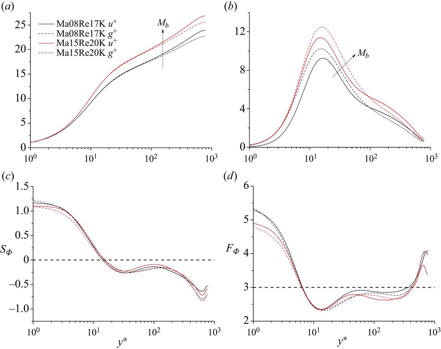
Figure 5. Variations of (a) the viscous-scaled mean statistics, (b) the second-order statistics, (d) the skewness, and (d) the flatness of  $u'$ and $g'$ as functions of $y^*$ for the cases Ma08Re17K and Ma15Re20K in D2 with different Mach numbers. All cases are of $Re_{\tau }^{*}\approx 780$.
More detailed scrutiny of their differences can be revealed by inspecting the spectra, which is carried out in figure 6. Figure 6(a) shows the premultiplied normalized spanwise spectra of  $u'$ and $g'$ at $y=0.14h$ and $y=0.3h$ for the case Ma15Re20K. The spectral peaks of $u'$ and $g'$ are identical, that is, $\lambda _{z}=0.7h$ and $\lambda _{z}=1.1h$ for $y=0.14h$ and $y=0.3h$, respectively. It suggests that the characteristic length scales of these two variables grow simultaneously as the increase of wall-normal height. One thing that merits discussion is that the peak magnitudes of $g'$ are smaller than those of $u'$, whereas at smaller wavelengths, the energy contents of $g'$ are larger. Figure 6(b) compares the spectra of $u'$ and $g'$ at $y=0.3h$. Particular attention is paid to the inertial range. It can be found that the celebrated $k_z^{-5/3}$ scaling can be traced in the $u'$ spectrum, whereas the spectrum of $g'$ exhibits $k_z^{-4/3}$ behaviour. This is consistent with the theoretical prediction for the passive scalar in shear flows (Lohse Reference Lohse1994), and has also been observed in an incompressible pipe flow at moderate Reynolds number (Pirozzoli et al. Reference Pirozzoli, Romero, Fatica, Verzicco and Orlandi2022). The current study shows that mild compressibility cannot alter this scaling, and the theoretical analysis is still applicable.
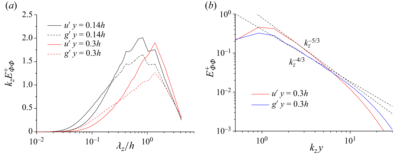
Figure 6. (a) Premultiplied normalized spanwise spectra of  $u'$ and $g'$ at $y=0.14h$ and $y=0.3h$ for the case Ma15Re20K; (b) normalized spanwise spectra of $u'$ and $g'$ at $y=0.3h$ for the case Ma15Re20K.
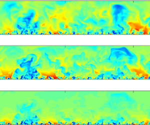
At last, it is sensible to take a look at the instantaneous flow fields of these two variables, which are shown in figure 7. Figures 7(a) and 7(b) display a  $z- y$ plane of $u^{\prime +}$ and $g^{\prime +}$ of the case Ma15Re20K, respectively. It can be seen that these two fields bear similar flow patterns in general. This observation is consistent with the spectra shown in figure 6(a). However, the scalar can be recognized to have sharper fronts, whereas the interfaces of $u'$ motions are coarser. This difference should be attributed to the PRF (Pirozzoli et al. Reference Pirozzoli, Bernardini and Orlandi2016). Its effects on the multiphysics couplings will be dissected in the next subsection.

Figure 7. Instantaneous normalized (a) streamwise velocity fluctuation  $u^{\prime +}$, and (b) passive scalar $g^{\prime +}$ contours in a $z- y$ plane of the case Ma15Re20K.
5.2. Multiphysics couplings
Before proceeding with the detailed analysis, it is better to have a rough idea of the overall picture of the multiphysics couplings. Figure 8(a) shows the distributions of  $RD_{\varPhi T}$ ( $\varPhi =u$ or $g$) for the cases Ma08Re17K and Ma15Re20K in D2. Notably, $RD_{u T}$ and $RD_{g T}$ are nearly identical within $y^*<10$. Although there are some gaps between the $RD_{uT}$ and $RD_{gT}$ profiles, they are relatively small compared with those in the logarithmic and outer regions. Therefore, it still can be accepted that $u'$ and $g'$ fields are coupled with $T'$ in the same degree in the viscous sublayer. However, prominent differences begin to emerge in the buffer layer and become significant in the logarithmic region. Taking the case Ma15Re20K as an example, $50\,\%$ and $88\,\%$ fluctuation intensity of $T'$ can be adequately captured by the linear couplings with $u'$ and $g'$ at $y_p^*\approx 100$, respectively. It underlines the fact that the influences originated from PRF decouple $u'$ and $T'$ evidently in the logarithmic and outer regions. On the contrary, $T'$ and $g'$ are coupled rather robustly in the whole channel. Conspicuously, there is still $50\,\%$ fluctuation intensity of $T'$ that can be satisfactorily captured by their coupling at the channel centre for Ma15Re20K. Apparently, the enlargement of the Mach number weakens the corresponding coherence. Figure 8(b) shows the variations of $RD_{u g}$ as functions of $y^*$. The magnitudes of $RD_{u g}$ increase rapidly in the logarithmic and outer regions. It shows once again that their coupling is diminished by the PRF in these regions. Figures 8(c) and 8(d) display the variations of $C_{\varPhi T}$ ( $\varPhi =u$ or $g$) and $C_{ug}$, respectively. As expected, $C_{u T}$ and $C_{u g}$ attenuate gradually beyond the viscous sublayer, whereas $C_{g T}$ only decay strikingly in the outer region. These observations are consistent with those of $RD_{\varPhi T}$ and $RD_{ug}$ shown in figures 8(a) and 8(b). In the following subsections, we will investigate the multiphysics couplings in the logarithmic and outer regions separately.
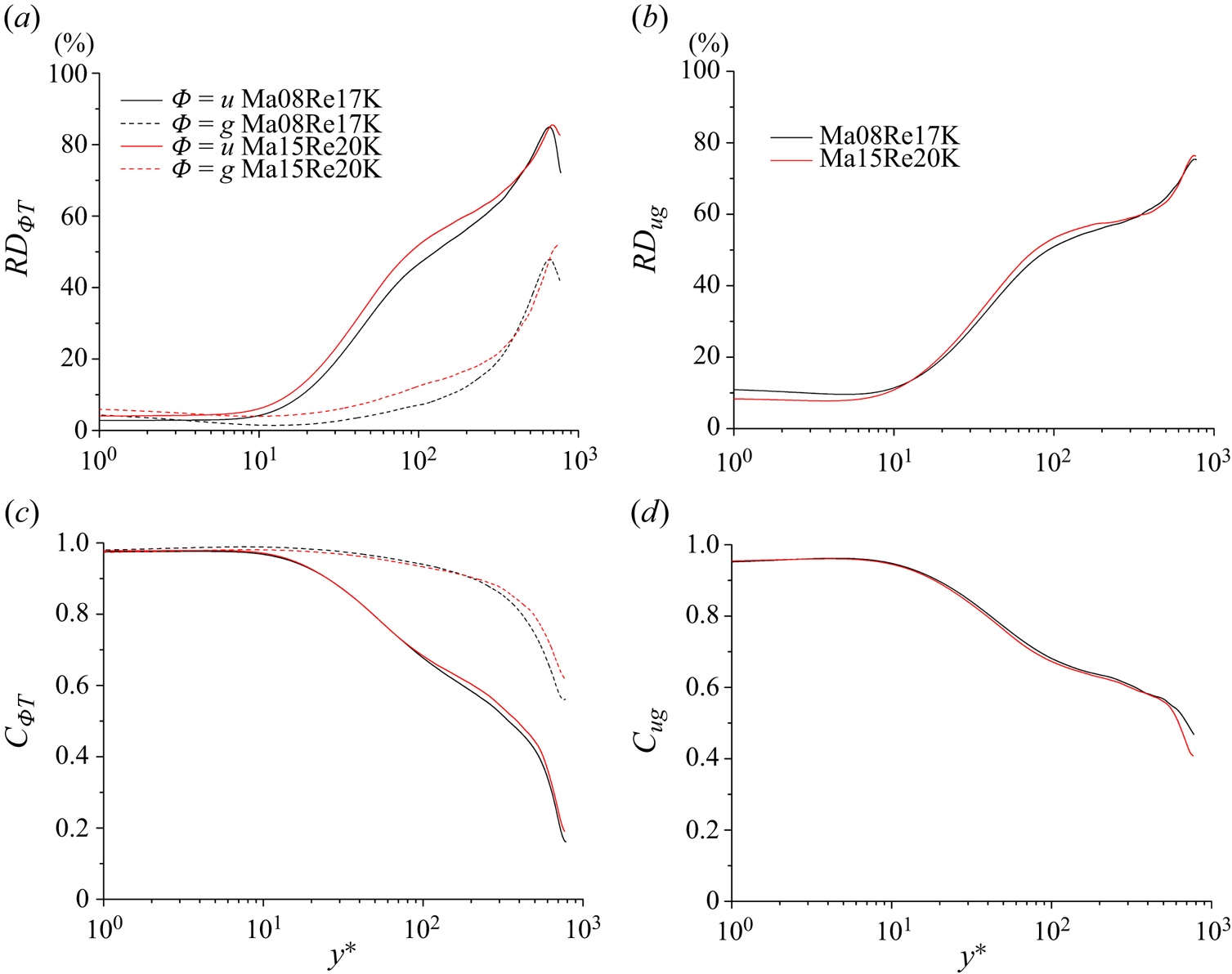
Figure 8. (a,b) Variations of (a)  $RD_{\varPhi T}$ and (b) $RD_{u g}$ as functions of $y^*$ for the cases Ma08Re17K and Ma15Re20K in D2; (c,d) variations of (c) $C_{\varPhi T}$ and (d) $C_{u g}$ as functions of $y^*$ for the cases Ma08Re17K and Ma15Re20K in D2.
5.2.1. Multiphysics couplings in the logarithmic region
The  $\gamma ^2_{u T}$ and $\gamma ^2_{g T}$ spectra of the case Ma15Re20K for $y^*=3.9\sqrt {Re_{\tau }^*}$ (namely the centre of the logarithmic layer (Mathis, Hutchins & Marusic Reference Mathis, Hutchins and Marusic2011), $y_m\approx 0.14h$ for Ma15Re20K) are displayed in figures 9(a) and 9(b), respectively. We recall from (3.3) that $\gamma ^{2}_{\varPhi T}$ is a measure of coherence between $T'$ and $\varPhi ^{\prime }$ at a given wall-normal position ( $\gamma ^{2}_{\varPhi T}=1$ indicates a prefect coherence, and $\gamma ^{2}_{\varPhi T}=0$ indicates no coherence). For $\gamma ^2_{u T}$, there exists only a small portion of the scale range where the LCS is prominent. This range is roughly bounded by
 \begin{equation} \lambda_x>\lambda_z,\quad \lambda_x>10y,\quad \lambda_z>2y. \end{equation}
Cheng & Fu (Reference Cheng and Fu2023a) pointed out that these range boundaries correspond to the length scales of the celebrated attached eddies (Marusic & Monty Reference Marusic and Monty2019). It hints at the fact that  $u'$ and $T'$ are linearly coupled at scales larger than those of the self-similar eddies. More fruitful discussion about this feature can be found in our previous work (Cheng & Fu Reference Cheng and Fu2023a), and is not given here. For $\gamma ^2_{g T}$, however, things are totally different. It is apparent that $g'$ and $T'$ are highly coupled at all scales, including the small-scale range. By comparison, it is not difficult to make a conclusion that the loss of the coherence between $T'$ and $u'$ at scales beyond (5.1a–c) should be ascribed to the effects originated from the pressure field, namely, the PRF. Hence, it is sensible to inspect the LCS associated with $p'$ and $T'$, which reads as
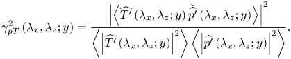 \begin{equation} \gamma^2_{p T}\left(\lambda_{x},\lambda_{z};y\right)=\frac{\left|\left\langle\widehat{T'}\left(\lambda_{x},\lambda_{z}; y\right) \breve{\widehat{p^{\prime}}}\left(\lambda_{x},\lambda_{z}; y_{}\right)\right\rangle\right|^2}{\left\langle\left|\widehat{T'}\left(\lambda_{x},\lambda_{z}; y\right)\right|^2\right\rangle\left\langle\left|\widehat{p'}\left(\lambda_{x},\lambda_{z}; y\right)\right|^2\right\rangle}. \end{equation}
Figure 9(c) presents its result at the same wall-normal position. Interestingly,  $\gamma ^2_{p T}$ is prominent at a scale range with low $\lambda _x$ ( $\lambda _x<\lambda _z$), beyond the boundaries given by (5.1a–c). This observation is reminiscent of some previous studies, which reported that $p'$ is more energetic at small scales (Tsuji et al. Reference Tsuji, Fransson, Alfredsson and Johansson2007; Tsuji, Marusic & Johansson Reference Tsuji, Marusic and Johansson2016; Cheng & Fu Reference Cheng and Fu2022b). For example, in our previous work (Cheng & Fu Reference Cheng and Fu2022b), we revealed that the scale feature of the self-similar $p'$ motions in supersonic channel flows can be characterized by $\lambda _{x}=1.8y$, which is significantly shorter than that of the self-similar $u'$ motions at a given wall-normal position, that is $\lambda _{x}=15.5y$. In this vein, the energetic $p'$ motions at small-scale range decouple $u'$ and $T'$ at these scales. Hence, there must be a mechanism to achieve this. We hypothesize that it is related to the self-sustaining process of the energy-containing eddies in the logarithmic region, and the relevant discussion is given in § 6.3. Figure 9(d) shows the distributions of $\gamma ^2_{u g}$. It can be seen that this spectrum is akin to that of $\gamma ^2_{u T}$ shown in figure 9(a). Especially, the boundaries of the energetic range are identical to those of $\gamma ^2_{u T}$. It indicates the similarities between $g'$ and $T'$, which will be discussed in § 6.1. The spectra obtained from the Ma08Re17K are similar, and we do not show them here for brevity.
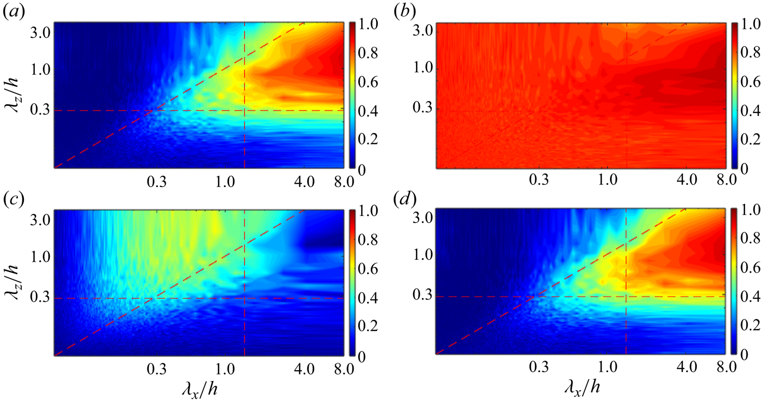
Figure 9. The (a)  $\gamma ^2_{u T}$, (b) $\gamma ^2_{g T}$, (c) $\gamma ^2_{p T}$ and (d) $\gamma ^2_{u g}$ spectra for the case Ma15Re20K when $y^*=3.9\sqrt {Re_{\tau }^*}$. The dashed oblique lines in (a,c,d) denote $\lambda _x=\lambda _z$, and the dashed transverse and the vertical lines denote $\lambda _z=2y$ and $\lambda _x=10y$, respectively.
Figure 10(a,c,e) shows the 2-D joint probability density functions (p.d.f.s) between  $u^{\prime +}$ and $T^{\prime +}$ (figure 10a), $u^{\prime +}$ and $g^{\prime +}$ (figure 10c) and $g^{\prime +}$ and $T^{\prime +}$ (figure 10e) when $y^*=3.9\sqrt {Re_{\tau }^*}$ for the case Ma15Re20K. The shapes of the p.d.f.s between $u^{\prime +}$ and $T^{\prime +}$, and $u^{\prime +}$ and $g^{\prime +}$ are both elliptical with dominance in the first and third quadrants. By contrast, the shape of the p.d.f. between $g^{\prime +}$ and $T^{\prime +}$ looks more like a straight line. These observations suggest that the correlations between $u^{\prime +}$ and $T^{\prime +}$ and $u^{\prime +}$ and $g^{\prime +}$ are not as strong as the one between $g^{\prime +}$ and $T^{\prime +}$ in the logarithmic region.
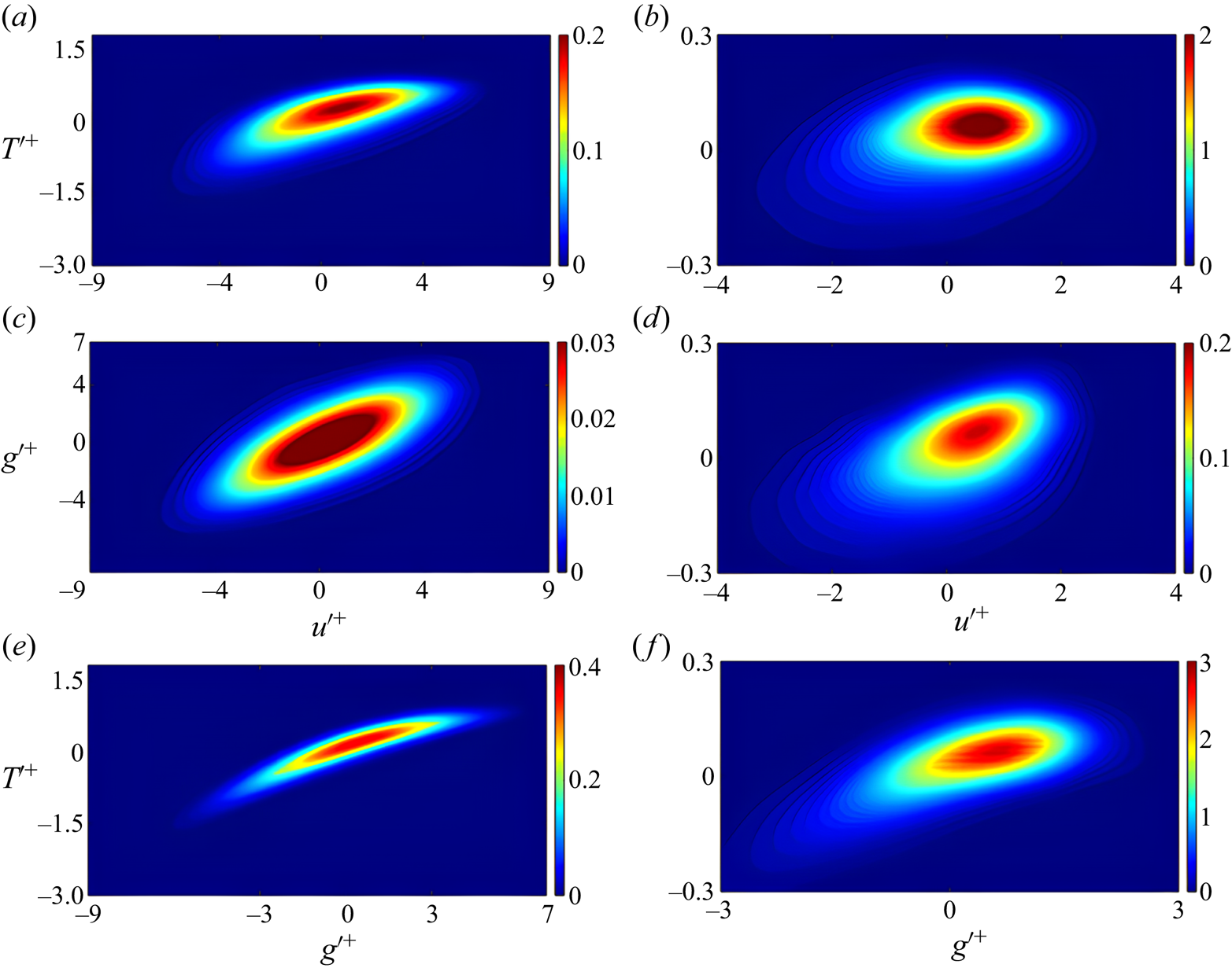
Figure 10. (a,c,e) The 2-D joint p.d.f.s between (a)  $u^{\prime +}$ and $T^{\prime +}$, (c) $u^{\prime +}$ and $g^{\prime +}$, (d) $g^{\prime +}$ and $T^{\prime +}$ when $y^*=3.9\sqrt {Re_{\tau }^*}$; (b,d,f) 2-D joint p.d.f.s of (b) $u^{\prime +}$ and $T^{\prime +}$, (d) $u^{\prime +}$ and $g^{\prime +}$, (f) $g^{\prime +}$ and $T^{\prime +}$ when $y=0.8h$. The data is taken from the case Ma15Re20K.
5.2.2. Multiphysics couplings in the outer region
According to the profiles of  $RD_{g T}$, $RD_{u T}$ and $RD_{u g}$ shown in figure 9, the coupling between $g'$ and $T'$ can be observed to be depressed in the outer region, and the counterpart of $u'$ and $T'$(
$T'$( $g'$) is the weakest within the whole boundary layer. Hence, it is intriguing to inspect this change by resorting to the SLSE. The results presented below are all collected at $y=0.8h$.
Figure 11(a) illustrates the  $\gamma ^2_{u T}$ spectrum of the case Ma15Re20K. Intriguingly, the spectrum is only non-trivial at the scale range corresponding to the VLSMs (Del Álamo & Jiménez Reference Del Álamo and Jiménez2003; Hutchins & Marusic Reference Hutchins and Marusic2007; Cheng et al. Reference Cheng, Li, Lozano-Durán and Liu2019), namely, $\lambda _x>4h$ and $\lambda _z>h$, which is significantly different from the scenario in the logarithmic region (see figure 9a). Combining the energetic range of $\gamma ^2_{u T}$ in the logarithmic region, we can conclude that $u'$ and $T'$ are coupled with the medium of the energy-containing motions at each wall-normal position. In other words, their coupling ties in with the energy-containing motions due to the presence of the PRF. Figure 12 shows the instantaneous fields of $u'^+$ (figure 12a), $g'^+$ (figure 12b) and $T'^+$ at $y=0.8h$ (figure 12c) in the case Ma15Re20K. The large-scale structures of $u'$ are visible, whereas for $g'$ and $T'$, they are not. In contrast, both $g'$ and $T'$ are characterized by spotted extreme events without discernible large-scale streaky shapes. Hence, in compressible channel flows, the large-scale structures of $g'$ with $\lambda _x>4h$ also do not dominate in the outer region when $Sc$ is close to unity, just like the scenario in incompressible cases (Abe et al. Reference Abe, Kawamura and Matsuo2004; Pirozzoli Reference Pirozzoli2023). The appearance of the coupling between $u'$ and $g'$ at the scales of the VLSMs does not indicate the dominance of the large-scale structures of $g'$ in the outer region. It only suggests that $u'$ and $g'$ are well-coherent in the scale range corresponding to the energy-containing motions in the outer region.
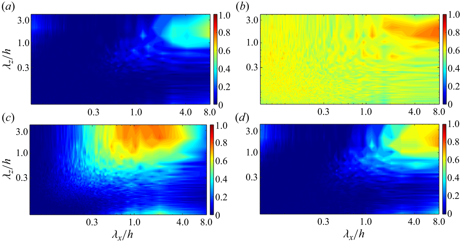
Figure 11. The (a)  $\gamma ^2_{u T}$, (b) $\gamma ^2_{g T}$, (c) $\gamma ^2_{p T}$ and (d) $\gamma ^2_{u g}$ spectra for the case Ma15Re20K when $y=0.8h$.
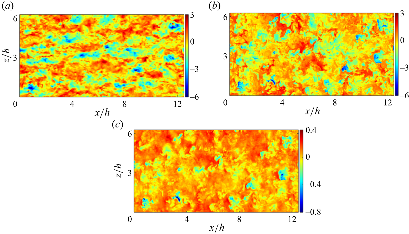
Figure 12. Top view of the instantaneous (a) streamwise velocity fluctuation  $u^{\prime +}$, (b) passive scalar fluctuation $g^{\prime +}$ and (c) temperature fluctuation $T^{\prime +}$ at $y=0.8h$.
On the other hand, though the coupling between  $g'$ and $T'$ is recognized to be diminished in the outer region, however, the driving mechanism behind it is totally different from that of $u'$ and $T'$, see the $\gamma ^2_{g T}$ spectrum in figure 11(b). Comparing with the $\gamma ^2_{g T}$ in the logarithmic region (figure 9b), the coherence between $g'$ and $T'$ at all scales is undermined but still maintained to be relatively large with $\gamma ^2_{g T}>0.5$. It underlines the fact that the coupling between $g'$ and $T'$ is not entirely related to the energy-containing motions. In § 6.1, we will dissect the relationship between the two variables. The $\gamma ^2_{p T}$ spectrum is shown in figure 11(c). It can be seen that the energetic scales are still shorter than those of $\gamma ^2_{u T}$, though they increase with the wall-normal height. This scenario is consistent with that in the logarithmic region, which implies that the effects of PRF are identical in these two zones. Figure 11(d) displays the $\gamma ^2_{u g}$ spectrum. It is akin to the $\gamma ^2_{u T}$ spectrum. It hints at the fact that $T'$ is a passive variable by and large, just like $g'$.
$g'$.
Figure 10(b,d,f) shows the 2-D joint p.d.f.s between  $u^{\prime +}$ and $T^{\prime +}$ (figure 10b), $u^{\prime +}$ and $g^{\prime +}$ (figure 10d) and $g^{\prime +}$ and $T^{\prime +}$ (figure 10f)when $y=0.8h$ for the case Ma15Re20K. From a general view, the shapes of all these p.d.f.s are elliptical. One thing worth noting is that the correlation between $g^{\prime +}$ and $T^{\prime +}$ is attenuated in the outer region, compared with the results in the logarithmic region (figure 10e). We will try to explain it in § 6.2.
In summary, analyses in § 5 shed light on the fact that the  $u-T$ and $u-g$ couplings at a given wall-normal height are maintained by the energy-containing motions populating this region, whereas the $g-T$ coupling is not. Most of the previous studies investigate the multiphysics couplings via the correlation function (Abe et al. Reference Abe, Kawamura and Matsuo2004; Abe & Antonia Reference Abe and Antonia2009; Gerolymos & Vallet Reference Gerolymos and Vallet2014). Though it can measure the degree of one coupling generally, it cannot reveal the relationship between this coupling and the multiscale energy-containing motions, as well as the underlying physical mechanism. By deploying the SLSE as a diagnostic tool, the present study has overcome this limitation.
6. Discussion
6.1. Relationship between temperature and passive scalar fields
Heretofore, the multiphysics couplings in the logarithmic and outer regions are revealed. We can appeal to the exhibited results to answer the questions raised in the introduction. Namely, if the temperature field in a compressible wall turbulence can be considered as a passive scalar in most cases, in which part of the boundary layer do the features of the temperature field depart from those of a passive scalar field most? These issues have never been addressed by previous studies.
For the first question, our answer is yes. The temperature field in the vast majority of zones in a channel can be treated roughly (not totally) as a passive scalar. The evidence is listed as follows.
(i) The $u-g$ coupling approaches the $u-T$ coupling, and the $g-T$ coupling is robust within the whole boundary layer. This outline is evident as per the RDs shown in figure 8. More details are revealed by the $\gamma ^2_{g T}$ spectra illustrated in figures 9(b) and 11(b), which are totally different from the $\gamma ^2_{u T}$ spectra. Concurrently, the $\gamma ^2_{u g}$ spectra display similar shapes with the $\gamma ^2_{u T}$ spectra.
(ii) The distributions of 2-D joint p.d.f.s between
$u^{\prime +}$ and $T^{\prime +}$ resemble those between $u^{\prime +}$ and $g^{\prime +}$ in the logarithmic and outer regions (see figure 10). This observation can be considered as a piece of evidence.(iii) The turbulent Prandtl number (
$Pr_t$) and Schmidt number ($Sc_t$) are of equal magnitudes in most regions of a boundary layer. Their definitions take the form of
(6.1)and\begin{equation} Pr_t=\frac{\overline{\rho v^{\prime} u^{\prime}} \partial_y \bar{T}}{\overline{\rho v^{\prime} T^{\prime}} \partial_y \bar{u}}, \end{equation}(6.2)The variations of these two parameters in the cases Ma08Re17K and Ma15Re20K of dataset D2 are shown in figure 13(a), and the empirical formula given by Abe & Antonia (Reference Abe and Antonia2017) for incompressible flow is included for comparison. This formula is in accordance with the DNS results for\begin{equation} Sc_t=\frac{\overline{\rho v^{\prime} u^{\prime}} \partial_y \bar{g}}{\overline{\rho v^{\prime} g^{\prime}} \partial_y \bar{u}}. \end{equation}$y>0.2h$. What is more, the magnitudes of $Sc_t$ of the two cases are approximately equal to those of $Pr_t$. Hence, there is no doubt that $T'$ behaves like $g'$ in turbulent transport. This perspective is also put forward in our previous study (Cheng & Fu Reference Cheng and Fu2023a). It is acceptable, since the typical structures of $T'$ and $g'$ are shown to be similar, even in the outer region, see figure 12.(iv) The length scales that are responsible for the variations of
$\gamma ^2_{u T}$ and $\gamma ^2_{u g}$ in the logarithmic region are identical. In Cheng & Fu (Reference Cheng and Fu2023a), we defined a $\gamma ^2_{u\varPhi }-$weighted average spanwise wavenumber $k_z^{\star }(y)$, and the corresponding length scale $\lambda _z^{\star }=2{\rm \pi} /k_z^{\star }(y)$. The former reads as
(6.3)where\begin{equation} k_z^{{\star}}(y)=\frac{\displaystyle\int\nolimits_{\varOmega} k_z \gamma_{u\varPhi}^2\left(y ; k_x, k_z\right) \mathrm{d} k_x \,\mathrm{d} k_z}{\displaystyle\int\nolimits_{\varOmega} \gamma_{u\varPhi}^2\left(y ; k_x, k_z\right) \mathrm{d} k_x \,\mathrm{d} k_z}, \end{equation}$\varOmega$ is the spectral domain defined by (5.1a–c), i.e. the energetic scale range of $\gamma ^2_{u T}$ and $\gamma ^2_{u g}$ in the logarithmic region. Thus, $\lambda _z^{\star }$ represents the length scale that is responsible for the variation of $\gamma ^2_{u\varPhi }$. Figure 13(b) shows the variations of $\lambda _z^{\star }/h$ with $\varPhi =T$ and $\varPhi =g$ as functions of $y/h$ in the logarithmic region for Ma15Re20K. It can be seen that there is a linear relationship between $\lambda _z^{\star }/h$ and $y/h$. This observation underscores the fact that the $T'$ and $g'$ fields are linearly coupled with $u'$ within the same self-similar scale range in the logarithmic region. Both the variations of $\gamma ^2_{u T}$ and $\gamma ^2_{u g}$ spectra along the wall-normal direction in the logarithmic region are chiefly ascribed to the self-similar eddies.(v) Figure 14(a) shows the normalized spanwise spectrum of
$T'$ at $y=0.3h$ for the case Ma15Re20K. The corresponding Taylor microscale Reynolds number $Re_{\lambda }$ is 79.2, based on the local mean density and the dynamic viscosity, which meets the requirement for developing the inertial range, namely, $Re_{\lambda }\geq 50$ (Motoori & Goto Reference Motoori and Goto2019). Interestingly, the spectrum exhibits a $k_z^{-4/3}$ scaling in the range of $1.3< k_zy<3.8$, and bears a $k_z^{-5/3}$ scaling in the range of $2.6< k_zy<9.8$, respectively. This observation is consistent with Lohse (Reference Lohse1994), who proposed that the spectrum of a passive scalar field in a high-Reynolds-number shear flow would exhibit $k_z^{-4/3}$ scaling, followed by a $k_z^{-5/3}$ range. It also provides compelling evidence in favour of the statement that $T'$ in compressible channel flows can be considered as a passive scalar. Figure 14(b) shows the normalized spanwise spectrum of $T'$ at $y=0.3h$ for the case Ma15Re9K in D2 ($Re_{\lambda }\approx 49.3$). It can be seen that only the $k^{-5/3}$ range is detectable. It suggests that only at high Reynolds numbers can the $k^{-4/3}$ scaling be traced.


Figure 13. (a) The  $Pr_t$ and $Sc_t$ as functions of $y/h$, and the empirical formula $Pr_t=0.9-0.3(y/h)^2$ given by Abe & Antonia (Reference Abe and Antonia2017) for incompressible flow is represented by blue line; (b) variation of $\lambda _z^{\star }/h$ as a function of $y_p/h$ in the logarithmic region for Ma15Re20K. In (b), the red dashed line denotes $\lambda _z^{\star }=3.6y$.

Figure 14. Normalized spanwise spectra of  $T'$ at $y=0.3h$ for the case ( $a$) Ma15Re20K and ( $b$) Ma15Re9K.
However, though  $T'$ performs like $g'$ in most regions of a channel at first glance, the effects of the interaction between the energy and momentum equations can also be monitored. The properties of $T'$ would deviate from those of $g'$ gradually in the logarithmic and outer regions in supersonic flows, especially, the zone in the vicinity of the channel centre. This is the answer to the second question. As a proof, the coupling between $g'$ and $T'$ is significantly weakened in the logarithmic and outer regions. This proposition can be validated by inspecting the distributions of $RD_{gT}$ shown in figure 8(a). In addition, it is not difficult to observe that $RD_{gT}$ of the cases Ma08Re17K and Ma15Re20K in D2 increase rapidly when $y^*>400$. The mechanism of this transition will be further clarified in § 6.2 by decomposing the temperature field into the acoustic and entropic modes.
6.2. Acoustic and entropic modes of temperature field
The Kovasznay decomposition is often adopted to decompose the thermodynamic variables into the acoustic and entropic modes under the condition of weak compressibility (Kovasznay Reference Kovasznay1953; Chassaing et al. Reference Chassaing, Antonia, Anselmet, Joly and Sarkar2002; Gauthier Reference Gauthier2017; Wang et al. Reference Wang, Wan, Chen, Xie, Wang and Chen2019). The acoustic mode of the temperature fluctuation is defined as (Chassaing et al. Reference Chassaing, Antonia, Anselmet, Joly and Sarkar2002; Gauthier Reference Gauthier2017)
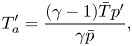 \begin{equation} T_a^{\prime}=\frac{(\gamma-1) \bar{T} p^{\prime}}{\gamma \bar{p}}, \end{equation}
and the entropic mode is given by  $T_e^{\prime }=T'-T_a^{\prime }$ (Chassaing et al. Reference Chassaing, Antonia, Anselmet, Joly and Sarkar2002; Gauthier Reference Gauthier2017). In this manner, the intensity of the temperature fluctuation can be decomposed as
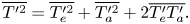 \begin{equation} \overline{T^{\prime 2}}=\overline{T_e^{\prime 2}}+\overline{T_a^{\prime 2}}+2\overline{T_e^{\prime}T_a^{\prime}}. \end{equation}
 Figure 15(a) shows the variations of the ratios  $\overline {T_a^{\prime 2}}/\overline {T^{\prime 2}}$, $\overline {T_e^{\prime 2}}/\overline {T^{\prime 2}}$, and $2\overline {T_e^{\prime }T_a^{\prime }}/\overline {T^{\prime 2}}$ of the cases Ma08Re17K and Ma15Re20K in D2. One observation is that the correlations $2\overline {T_e^{\prime }T_a^{\prime }}/\overline {T^{\prime 2}}$ of the two cases are only non-negligible in the vicinity of the wall and the outer region. Undoubtedly, the interaction between the modes is pronounced in these two regions, which is in accordance with the proposition that the two modes are not statistically independent, and can interact with each other (Kovasznay Reference Kovasznay1953). Another prominent observation is that the magnitudes of the acoustic modes in the two cases are gradually increasing in the logarithmic and outer regions. For the supersonic case Ma15Re20K, the magnitude of the acoustic mode approaches that of the entropic mode near the channel centre. We notice that this scenario bears some similarities with the variation tendencies of $RD_{g T}$ shown in figure 8. It may suggest that the deviation of the properties of $T'$ from a pure passive scalar in the logarithmic and outer regions is related to the enhanced acoustic mode. Hence, it is of interest to investigate the couplings of the two modes with $g'$ separately to shed light on this effect.
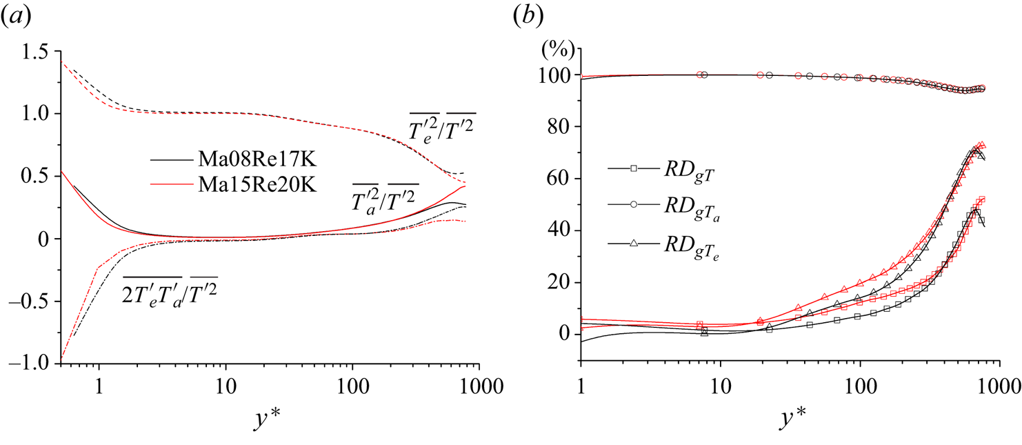
Figure 15. (a) Variations of the ratios  $\overline {T_a^{\prime 2}}/\overline {T^{\prime 2}}$, $\overline {T_e^{\prime 2}}/\overline {T^{\prime 2}}$ and $2\overline {T_e^{\prime }T_a^{\prime }}/\overline {T^{\prime 2}}$ of the cases Ma08Re17K and Ma15Re20K in D2; (b) variations of $RD_{g T}$, $RD_{g T_a}$ and $RD_{g T_e}$ of the cases Ma08Re17K and Ma15Re20K in D2.
Figure 15(b) shows the variations of  $RD_{g T}$, $RD_{g T_a}$ and $RD_{g T_e}$, and figure 16 displays the $\gamma ^2_{g T_a}$ (figure 16a,c) and $\gamma ^2_{g T_e}$ (figure 16b,d) spectra at two selected wall-normal positions in the logarithmic and outer regions. The following comments can be made with regard to these two figures.
(i) Here
$RD_{g T_a}\approx 100\,\%$ within the whole channel indicates that the acoustic mode is not coherent with the passive scalar at all. Moreover, the energetic regions in $\gamma ^2_{g T_a}$ spectra (figure 16a,c) at the two selected wall-normal positions collapse with those of $\gamma ^2_{p T}$ shown in figures 9(c) and 11(c). These observations are consistent with the mechanisms of the acoustic mode (Kovasznay Reference Kovasznay1953).(ii) The magnitudes of
$\gamma ^2_{g T_e}$ shown in figure 16(b,d) bear a strong similarity to those of $\gamma ^2_{g T}$ in figures 9(b) and 11(d). It underlines the fact that the coherence between $T'$ and $g'$ fields is dominated by the entropic mode of $T'$.(iii) The magnitudes of
$RD_{g T_e}$ are larger than those of $RD_{g T}$ in the logarithmic and outer regions. This observation signifies that $T_e'$ is also not a pure passive scalar like $g'$. In fact, Eyink & Drivas (Reference Eyink and Drivas2018) already revealed that the entropy in compressible turbulence is not a pure passive scalar via theoretical analysis. This is not good news for turbulence modelling, as it shows that the temperature field in compressible wall-bounded turbulence is rather intricate.(iv) The larger magnitudes of
$RD_{g T_e}$ in the outer region than those of $RD_{g T}$ also indicates that the interaction between $T_e'$ and $T_a'$ contributes to the $T-g$ coupling. It is consistent with the results displayed in figure 15(a) that the ratios $2\overline {T_e^{\prime }T_a^{\prime }}/\overline {T^{\prime 2}}$ are non-trivial in the outer region.


Figure 16. The (a)  $\gamma ^2_{g T_a}$, (b) $\gamma ^2_{g T_e}$ spectra at $y^*=3.9\sqrt {Re_{\tau }^*}$; (c) $\gamma ^2_{g T_a}$ and (d) $\gamma ^2_{g T_e}$ spectra at $y=0.8h$ for the case Ma15Re20K.
In summary, the key finding of this subsection is that the deviation of  $T'$ from a pure passive scalar in the logarithmic and outer regions is chiefly due to the acoustic mode. Furthermore, the entropic mode is not a pure passive scalar, and the interaction between the two modes also contributes to the coupling between $T'$ and $g'$. The degree of the $g-T$ couplings is the outcome of their combined effects.
6.3. Relationship between pressure and velocity fields
Up to now, a remaining question has not been answered, i.e. how does the PRF affect the streamwise velocity fluctuation and drive it away from a passive scalar (like  $g'$ or $T'$)? We notice that $u'$ is highly linked with $T'$ ( $g'$) within the scales corresponding to the energy-containing eddies in the logarithmic and outer regions (see figures 9 and 11). Hence, we hypothesize that it is the role PRF plays in the self-sustaining process of these eddies that leads to the decoupling of $u'$ and $T'$ ( $g'$) at smaller scales.
It is gradually admitted by the turbulence community that the energy-containing eddies in the logarithmic and outer regions bear an analogous self-sustaining process as the near-wall turbulence (Flores & Jiménez Reference Flores and Jiménez2010; de Giovanetti, Hwang & Choi Reference de Giovanetti, Hwang and Choi2016; Hwang & Bengana Reference Hwang and Bengana2016; Lozano-Durán, Bae & Encinar Reference Lozano-Durán, Bae and Encinar2020). It is generally accepted that the so-called self-sustaining process is composed by three steps. First, the streaks are amplified by the streamwise vortices via the lift-up effect, and the energy is transferred from the mean shear to the  $u'$ (Landahl Reference Landahl1990; Kim & Lim Reference Kim and Lim2000; Hwang & Cossu Reference Hwang and Cossu2010); second, the amplified streaks would break down due to secondary instability or transient growth (Hamilton, Kim & Waleffe Reference Hamilton, Kim and Waleffe1995; Schoppa & Hussain Reference Schoppa and Hussain2002); third, the streamwise vortices would be generated under the nonlinear mechanisms (Hamilton et al. Reference Hamilton, Kim and Waleffe1995; Schoppa & Hussain Reference Schoppa and Hussain2002). The pressure field is directly involved in the third step (Cho, Hwang & Choi Reference Cho, Hwang and Choi2018; Kawata & Tsukahara Reference Kawata and Tsukahara2021), and detailed discussion is given as follows.
In a statistically steady compressible wall turbulence, the Reynolds stress equation takes the form of
 \begin{equation} 0=C_{i j}+P_{i j}+D_{i j}+\varPi_{i j}-\varPhi_{\epsilon_{i j}}+M_{i j}, \end{equation}
where  $C$,
$C$,  $P$,
$P$,  $D$,
$D$,  $\varPi$, $\varPhi _{\epsilon }$ and $M$ denote the advection, production, viscous diffusion, pressure-strain correlation, viscous dissipation and mass flux associated with density fluctuations, respectively. The pressure field is mainly included in the pressure-strain term, which reads as
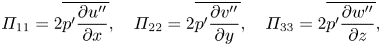 \begin{equation} \varPi_{11}=2\overline{p^{\prime} \frac{\partial u^{\prime \prime}}{\partial x}}, \quad \varPi_{22}=2\overline{p^{\prime} \frac{\partial v^{\prime \prime}}{\partial y}}, \quad \varPi_{33}=2\overline{p^{\prime} \frac{\partial w^{\prime \prime}}{\partial z}}, \end{equation}
for the streamwise ( $\overline {\rho u^{\prime \prime } u^{\prime \prime }}$), wall-normal ( $\overline {\rho v^{\prime \prime } v^{\prime \prime }}$) and spanwise ( $\overline {\rho w^{\prime \prime } w^{\prime \prime }}$) turbulence intensities, respectively.
Figure 17(a) shows the variations of  $\varPi _{11}^+$, $\varPi _{22}^+$ and $\varPi _{33}^+$ as functions of $y/h$ in the case Ma15Re20K of D2, and the profile of $-(\varPi _{22}^++\varPi _{33}^+)$ is also included for comparison. It can be seen that only $\varPi _{11}^+$ is negative, whereas both $\varPi _{22}^+$ and $\varPi _{33}^+$ are positive throughout the logarithmic and outer regions. Furthermore, the relation, $\varPi _{11}^++\varPi _{22}^++\varPi _{33}^+\approx 0$, is strictly kept in the logarithmic and outer regions. On the other hand, for the wall-normal and spanwise turbulence intensities, their production terms do not exist. It indicates that the pressure-strain correlations play an important role in the turbulence kinetic energy (TKE) redistribution; especially, as only $\varPi _{11}^+<0$, $\varPi _{11}^+$ plays a leading role in transferring TKE to other velocity components. The percentage of energy produced in the streamwise direction transferred to the other components can be measured by calculating the ratio (Duan, Beekman & Martin Reference Duan, Beekman and Martin2010)
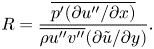 \begin{equation} R=\frac{\overline{p^{\prime} (\partial u^{\prime \prime}/ \partial x)}}{\overline{\rho u^{\prime \prime} v^{\prime \prime}} (\partial \tilde{u}/\partial y)}. \end{equation}
Figure 17(b) shows the variations of  $R$ as functions of $y^*$ in the case Ma15Re20K and Ma08Re17K of D2. It can be seen that $R$ is nearly constant in the logarithmic region for a selected case and is not sensitive to the magnitude of $M_b$. It suggests that the TKE redistribution is a typical mechanism in this region. On the other hand, it is well known that the streamwise vortices are the dominant carriers of the wall-normal velocity fluctuations (Hwang Reference Hwang2015; Cheng et al. Reference Cheng, Li, Lozano-Durán and Liu2019), hence, it can be speculated that the interaction between the pressure field $p'$ and $\partial u^{\prime \prime }/\partial x$ draws TKE from $u'$ and injects it into the streamwise vortices. As a consequence, the coherence between $u'$ and $g'$(
$g'$( $T'$) is diminished at the scales corresponding to the streamwise vortices. This is the scenario shown in figures 9 and 11. To further reveal their relationship quantitatively, we define a correlation function between the instantaneous pressure strain $p_s=2p^{\prime } \partial u^{\prime \prime }/\partial x$ and the wall-normal fluctuation, that is,
 \begin{equation} C_{p_s v}=\frac{\left\langle p_s v^{\prime}\right\rangle}{p_{s,rms} v_{rms}^{\prime}}. \end{equation}
Figure 17(c) plots the distributions of  $C_{p_s v}$ as functions of $y^*$ for the case Ma15Re20K and Ma08Re17K of D2. In the logarithmic region, $C_{p_s v}$ of the two cases are negative. It is worth noting that the mean $p_s$ (i.e. $\varPi _{11}$) of a given case is also negative in the logarithmic region (see figure 17a). It indicates that $p_s$ is actively correlated with the positive $v'$ in this region. Figures 18(a) and 18(b) display the contours of instantaneous $u^{\prime +}$ (colour) and $g^{\prime +}$ (colour) in the logarithmic region $y^*=3.9\sqrt {Re_{\tau }^*}$ of a subdomain of the case Ma15Re20K, respectively. The contour of $v'^+$ (line) is also included in figure 18(a). It can be found that the majority of the flawed similarities between $u^{\prime +}$ and $g^{\prime +}$ can be traced in the regions where $v'$ is positive. This scenario is in sync with the values of $C_{p_s v}$ in the logarithmic region.
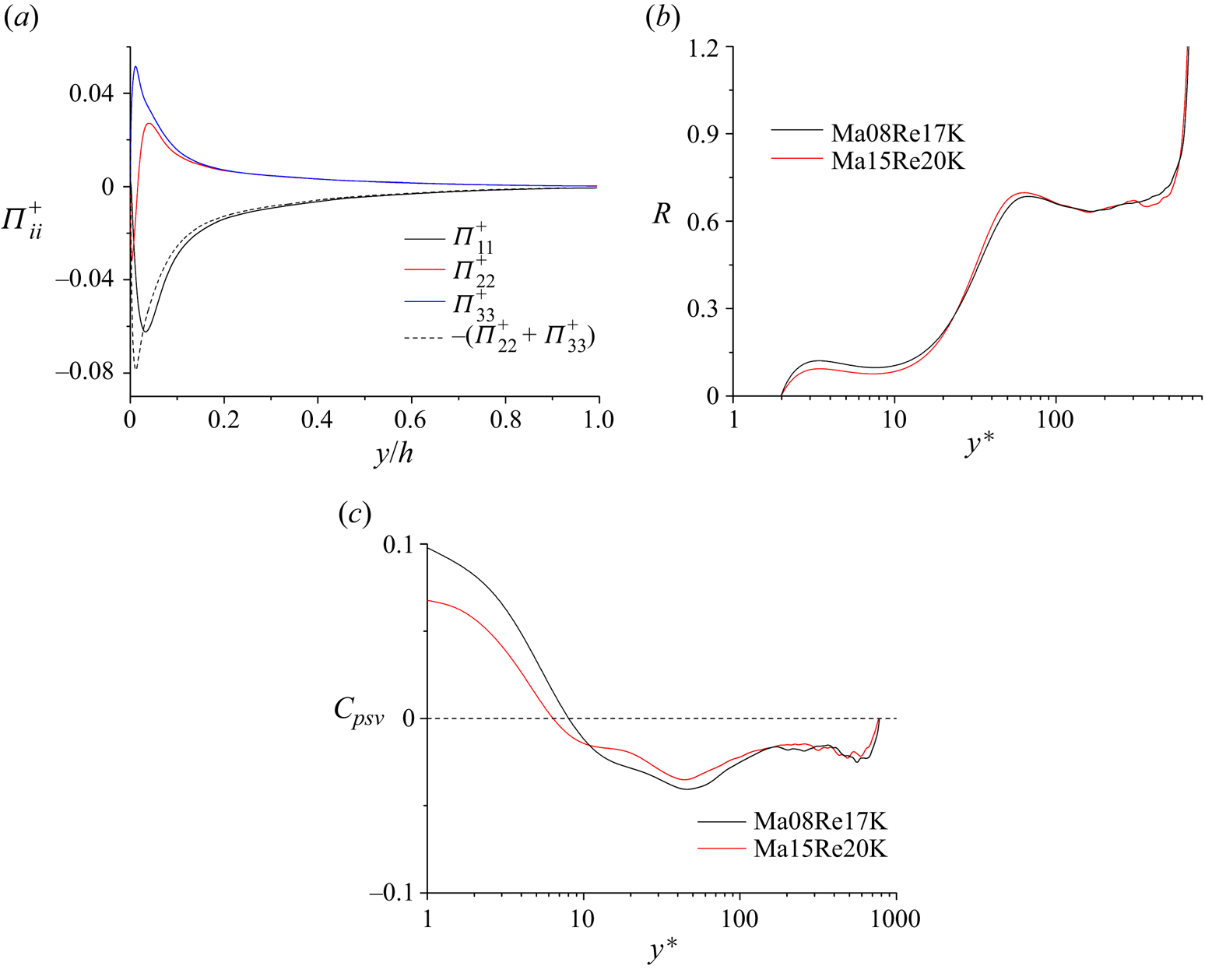
Figure 17. (a) Variations of  $\varPi _{11}^+$, $\varPi _{22}^+$ and $\varPi _{33}^+$ as functions of $y/h$ in the case Ma15Re20K of D2; (b,c) variations of (b) the ratio of streamwise pressure-strain term to production $R$ and (c) the correlation between the pressure strain and the wall-normal fluctuation $C_{p_s v}$ as functions of $y^*$.
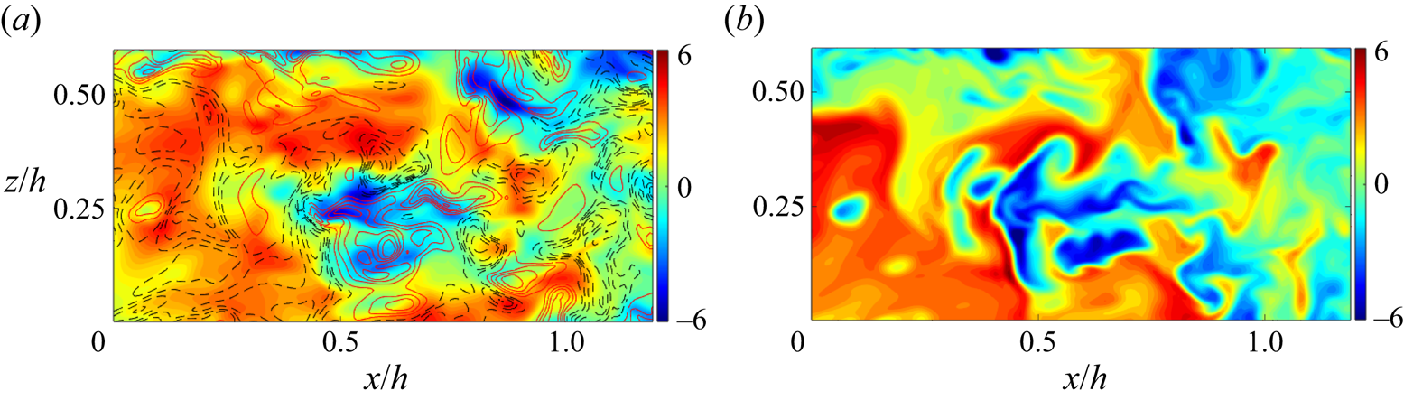
Figure 18. Instantaneous contours of (a)  $u^{\prime +}$ (colour) and (b) $g^{\prime +}$ (colour) in the logarithmic region $y^*=3.9\sqrt {Re_{\tau }^*}$ of a subdomain of the case Ma15Re20K. In panel (a), the contours of $v'^+$ (line) is also included; red solid and black dashed lines refer to positive and negative values of $v^{\prime +}$, respectively; the line increment is 1.5.
Figure 19 shows the premultiplied 2-D spectra of  $v'$ and $p'$ at $y^*=3.9\sqrt {Re_{\tau }^*}$, and $y=0.8h$. It can be observed that each spectrum is energetic at the scale range where the magnitudes of $\gamma ^2_{u T}$ and $\gamma ^2_{u g}$ are low. Furthermore, the spectral shape of $v'$ resembles that of $p'$ at a given wall-normal position. These observations are consistent with the analyses above. Moreover, the role of PRF can be hypothesized to be unchanged in the logarithmic and outer regions of low-speed wall turbulence or turbulent boundary layers at higher Mach numbers. As proofs, Gerolymos & Vallet (Reference Gerolymos and Vallet2023) showed very recently that the viscous-scaled variances of $p'$ are universal in the logarithmic and outer regions of turbulent channel flows at a wide range of Mach numbers. Abe & Antonia (Reference Abe and Antonia2009) also reported that flawed similarities between $u'$ and $g'$ can be traced in the regions where the streamwise pressure gradient is large due to the existence of the near-wall vortices in incompressible channel flows. This scenario is also in line with our analyses here. In fact, in incompressible wall turbulence, previous studies have already observed that the pressure-strain terms are closely related to the regeneration of the streamwise vortices in the self-sustaining process of energy-carried eddies at a given length scale (Cho et al. Reference Cho, Hwang and Choi2018; Kawata & Tsukahara Reference Kawata and Tsukahara2021). For example, Kawata & Tsukahara (Reference Kawata and Tsukahara2021) observed that the instantaneous pressure-strain term of streamwise TKE is significant when low-speed streaks are wavy with the evolutionary streamwise vortices in a Couette flow. However, none of these studies connects this mechanism to the $u-T$ and $u-g$ couplings. To the best knowledge of the authors, the present study clarifies it for the first time. As a side note, $\varPi _{11}^++\varPi _{22}^++\varPi _{33}^+=0$ can be found to be not strictly maintained in the near-wall region where compressibility is non-negligible. For incompressible wall turbulence, this relation is well-established due to the continuity. This is one of the main differences between these two kinds of flows.
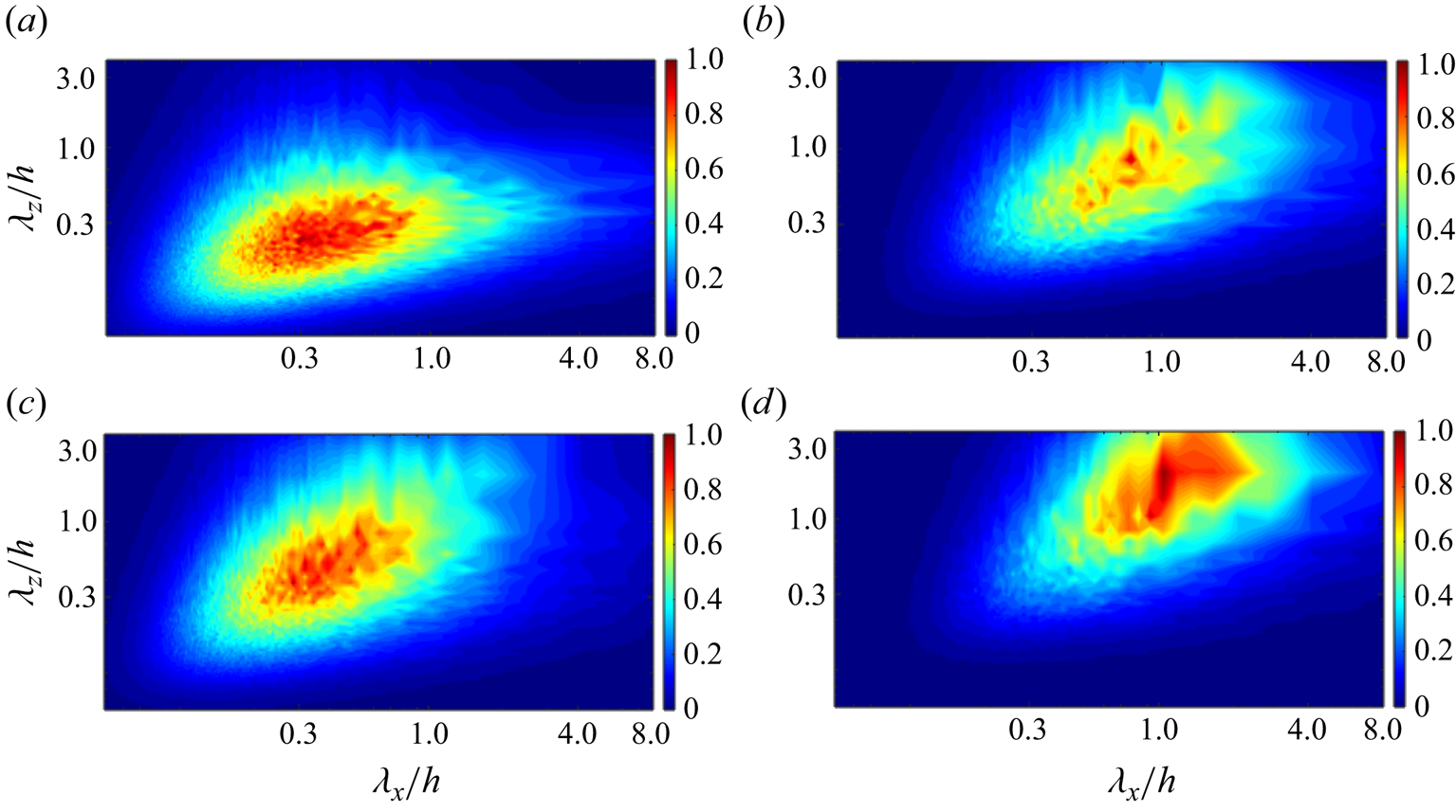
Figure 19. (a,b) Premultiplied 2-D spectrum of  $v'$ at (a) $y^*=3.9\sqrt {Re_{\tau }^*}$, and (b) $y=0.8h$ for Ma15Re20K; (c,d) premultiplied 2-D spectrum of $p'$ at (c) $y^*=3.9\sqrt {Re_{\tau }^*}$, and (d) $y=0.8h$ for Ma15Re20K. Each spectrum is normalized by its maximum value.
Though the present study only takes the compressible wall turbulence into consideration, the performance of the  $u-T$ coupling in the incompressible flows can also be predicted by leveraging the findings of the present study. According to the analyses above, the coupling between the streamwise velocity fluctuation and the passive scalar at a given wall-normal height is maintained by the energy-containing motions populating this region. Furthermore, the temperature field is a pure passive scalar in incompressible flows (Kim & Moin Reference Kim and Moin1989; Kawamura et al. Reference Kawamura, Abe and Matsuo1999; Abe et al. Reference Abe, Kawamura and Matsuo2004), and the self-sustaining process is similar in incompressible and compressible flows. Hence, the variation of the degree of the $u-T$ coupling in incompressible wall turbulence would follow that of the $u-g$ coupling reported in the present study, just as the results shown in figures 8(b) and 8(d). Namely, it would be gradually undermined as the wall-normal height increases. In the spectral space, the $u-T$ coupling would be only strong at the scales corresponding to the energy-containing motions residing in this wall-normal position, just like results shown in figures 9 and 11.
6.4. Reynolds-number and Mach-number effects on the multiphysics couplings
In § 4.2, we have concluded that the magnitude of the Reynolds number is the vital shaping factor for the  $u-T$ coupling. In this subsection, we are dedicated to investigating the Reynolds-number and Mach-number effects on the $u-g$ and $g-T$ couplings by leveraging dataset D2.
Figures 20(a) and 20(b) show the distributions of  $R_{ug}$ and $C_{ug}$ in dataset D2, respectively. A notable aspect discernible in the two figures is that the cases with similar $Re_{\tau }^*$ share like profiles of the two functions. This scenario is reminiscent of those of $u-T$ coupling displayed in figure 3. This is attributed to the fact that both $u-T$ and $u-g$ couplings at a given wall-normal position are maintained by the energy-containing motions residing in this region, according to our analyses above. On the other hand, the magnitude of the Reynolds number determines the degree of scale separation. Therefore, the Reynolds number is a key parameter in controlling the $u-g$ coupling, rather than the Mach number, at least within the cases under investigation.
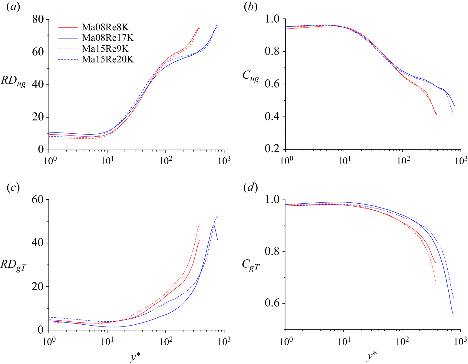
Figure 20. (a,c) Distributions of (a)  $R_{ug}$ and (c) $R_{gT}$ in the dataset D2; (b,d) distributions of (b) $C_{ug}$ and (d) $C_{gT}$ in the dataset D2.
Figures 20(c) and 20(d) display the variations of  $R_{gT}$ and $C_{gT}$ in dataset D2, respectively. It is apparent that the Reynolds number has more remarkable effects on this coupling. For a fixed $M_b$, the enlargement of the Reynolds number weakens the degree of the $g-T$ coupling in the outer regions and enhances it in the logarithmic region. For a given $Re_{\tau }^*$, the effects of increasing $M_b$ are not that obvious. In § 6.2, we demonstrate that the $g-T$ coupling is not sustained by the energy-containing motions, but dependent on the competition among the acoustic and entropic modes of the temperature field, as well as their interaction. Each component is highly correlated with the degree of $g-T$ coupling. As a result, the $g-T$ coupling is more intricate than the $u-T$ and $u-g$ couplings.
7. Concluding remarks
In the present study, through conducting numerical simulations and employing the SLSE and the correlation function as diagnostic tools, the multiphysics couplings in compressible channel flows are dissected. Particular attention is paid to the differences between the streamwise velocity and passive scalar fields. Additionally, the relationship between the passive scalar and temperature fields is also clarified. The key findings are summarized below.
(i) The VRF, namely, the difference between the viscous terms of the streamwise momentum and passive-scalar transport equations, only results in the distinct intermittent behaviours of
$u'$ and $g'$ in the near-wall region and rarely influences the multiphysics couplings in the whole boundary layer.(ii) The multiphysics couplings in the logarithmic and outer regions are highly linked with the inclusion of the pressure field in the streamwise momentum equation. The mean, fluctuating and high-order statistics of
$u'$ and $g'$ in these two regions are disparate. Their spectra in the inertial region also exhibit different scaling laws.(iii) In the logarithmic region, the
$u-T$ and $u-g$ couplings are found to be tight at the scales that correspond to the attached eddies and the VLSMs, whereas the $g-T$ coupling is robust in the whole spectral domain. In the outer region, the $u-T$ and $u-g$ couplings are only active at the scales corresponding to the VLSMs, whereas the $g-T$ coupling is diminished but still strong at all scales.(iv) The temperature field in the vast majority of zones in a channel can be treated roughly as a passive scalar. However, its physical properties gradually deviate from those of a pure passive scalar as the normal height increases due to the acoustic mode. Moreover, detailed analyses indicate that the entropic mode is not a pure passive scalar, and the interaction between the two modes also contributes to the
$g-T$ coupling.(v) The pressure field is involved in the regeneration of the streamwise vortices in the self-sustaining process of the logarithmic and outer regions. In this stage, the pressure-strain correlation of
$u'$ component plays a leading role in transferring TKE to other velocity components. As a consequence, the coherence between $u'$ and $g'$($T'$) is diminished at the scales corresponding to the streamwise vortices.(vi) The Reynolds number acts as a key parameter in shaping the
$u-T$ and $u-g$ couplings. These two couplings at a given wall-normal position are highly linked with the energy-containing motions populating this region. The enlargement of the Reynolds number would result in a more significant scale separation and thus intensify the couplings. For a fixed $M_b$, the enlargement of the Reynolds number weakens the degree of the $g-T$ coupling in the outer regions and enhances it in the logarithmic region.


Though the similarities between the temperature and passive scalar fields are reported broadly in a wide variety of the literature, the current study demonstrates that the dynamical interaction between the energy and momentum equations can inevitably lead to the differences between them in compressible wall turbulence. At last, we hypothesize that the size of the differences is related to the geometry of the flow. For a turbulent channel flow, the acoustic mode in the outer region would be more significant than a turbulent boundary layer with similar Mach number and wall temperature, because the geometrical features of an internal flow would result in the accumulation of the acoustic perturbations. If this is true, it suggests that the temperature field in compressible wall turbulence is rather complicated. More approaches are needed to analyse its physical behaviour and pave the way for its modelling.
Acknowledgements
The work is indebted to the encouragement of an anonymous reviewer of our previous paper (Cheng & Fu, J. Fluid Mech., vol. 964, 2023, A15). We are grateful to them for the insight on this interesting topic.
Funding
L.F. acknowledges the fund from the Research Grants Council (RGC) of the Government of Hong Kong Special Administrative Region (HKSAR) with RGC/ECS Project (no. 26200222), RGC/GRF Project (no. 16201023) and RGC/STG Project (no. STG2/E-605/23-N), the fund from Center for Ocean Research in Hong Kong and Macau, a joint research centre between Laoshan Laboratory and HKUST and the fund from the Project of Hetao Shenzhen–Hong Kong Science and Technology Innovation Cooperation Zone (no. HZQB-KCZYB-2020083).
Declaration of interests
The authors report no conflict of interest.
Data availability statement
The data that support the findings of this study are available from the corresponding author upon reasonable request.
Appendix A. Code validation
This appendix provides an example to demonstrate the code validation in the context of a passive scalar in compressible channel flow by simulating the reference case reported by Friedrich et al. (Reference Friedrich, Foysi and Sesterhenn2006) with (2.1). The Mach number and Reynolds number of the case are 1.5 and 3000, respectively, and  $Pr$ and $Sc$ are set as 0.7 and 1.0, respectively. The wall boundary condition of the passive scalar transport equation is
 \begin{equation} g(x,0,z,t)=1, \quad g(x,2h,z,t)={-}1, \end{equation}
which indicates the passive scalar is injected at the lower wall ( $\kern 1.5pt y=0$) with vanishing momentum and removed through the upper wall ( $\kern 1.5pt y=2h$). Other set-ups are identical to those described in § 2. Figures 21(a) and 21(b) show the variations of the mean and r.m.s. statistics of the scalar as functions of $y/h$, and the results of Friedrich et al. (Reference Friedrich, Foysi and Sesterhenn2006) are added for comparison. It can be seen that the results of the present study agree well with those of Friedrich et al. (Reference Friedrich, Foysi and Sesterhenn2006), which confirms the accuracy of the present code.
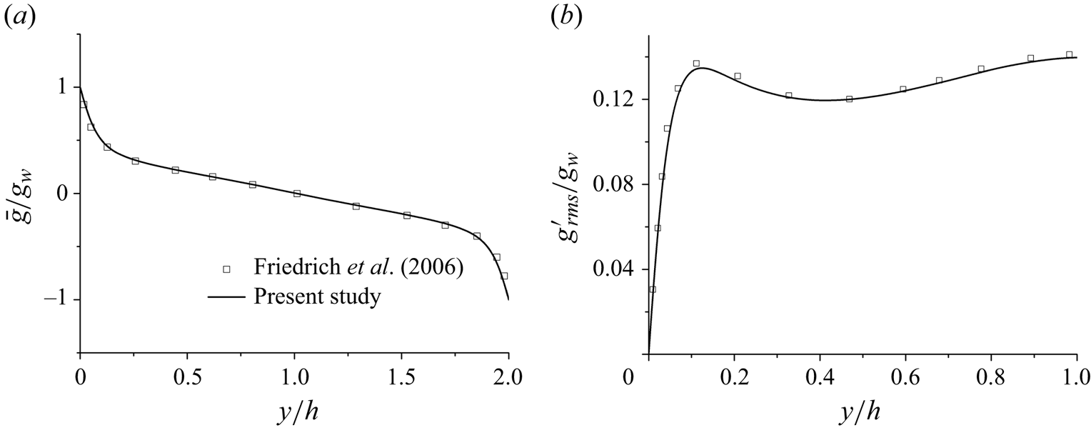
Figure 21. Variations of the (a) mean and (b) r.m.s. scalar statistics as functions of  $y/h$.
Appendix B. Effects of the grid resolution on the statistical properties of passive scalar and the related multiphysics couplings
The effects of the grid resolution on the statistical properties of passive scalar and the related multiphysics couplings are investigated. We concentrate on the case Ma08Re17K in dataset D2, because its grid resolution is the coarsest. The grid used here in the streamwise direction is two times finer than the original grid listed in table 2. They are denoted as fine and coarse cases hereafter, respectively. Other settings and parameters are the same.
Figures 22(a) and 22(b) compare the variations of the viscous-scaled mean and r.m.s. statistics of the scalar. The results of the fine and coarse cases agree well with each other. Figure 22(c) displays the distributions of  $C_{ug}$ and $C_{gT}$ of the two cases. It can be observed that their profiles agree reasonably well with each other. Figure 22(d) shows the normalized streamwise spectra of $g'$ at $y=0.8h$. Apparently, the spectra of the two cases collapse well in the shear-dominant and inertial regions, whereas the energy of the dissipative-range motions is better resolved in the fine case. Our results shown in the main body demonstrate that the $u-g$ coupling is maintained by the energy-containing eddies, not the dissipative-range ones. All these suggest that the grid resolutions shown in table 2 are sufficient for resolving the typical structures of the passive scalar and their associated multiphysics couplings when $Sc=1$.

Figure 22. (a,b) Variations of the (a) mean and (b) r.m.s. scalar statistics as functions of  $y^+$ for the fine and coarse cases; (c) distributions of $C_{ug}$ and $C_{gT}$ of the fine and coarse cases; (d) normalized streamwise spectra of $g'$ at $y=0.8h$ of the fine and coarse cases.
Appendix C. Comparison between $1-RD_{\varPhi T}$ and $C_{\varPhi T}$


The consistency between  $1-RD_{\varPhi T}$ and $C_{\varPhi T}$ is demonstrated by plotting them together in this appendix. Figure 23 shows their variations for the case Ma15Re3K in dataset D1. Both the values of these two quantities approach unity in the near-wall region, and begin to decay beyond $y/h>0.1$. Although their definitions are not the same, their variation tendencies are similar. They can be deployed as two metrics of the intensities of the multiphysics couplings.

Figure 23. Variations of  $C_{\varPhi T}$ and $1-RD_{\varPhi T}$ as functions of $y/h$ for the case Ma15Re3K in dataset D1.


 Open access