2 Experimental results and discussion

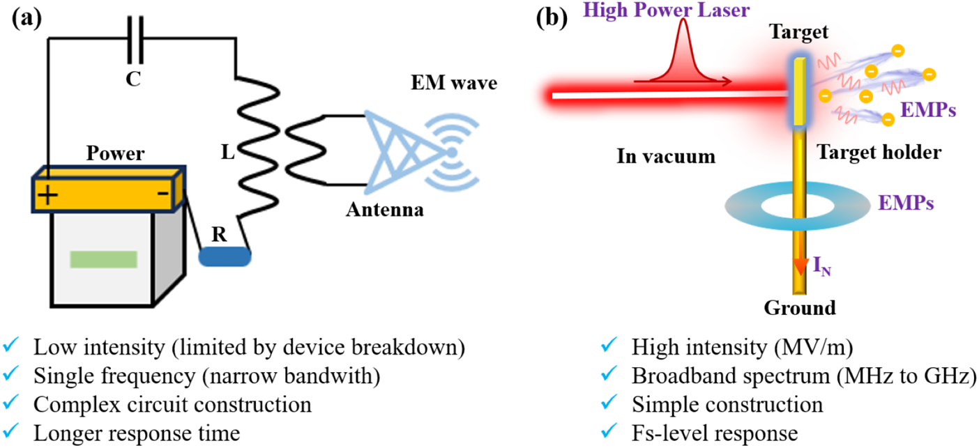
Figure 1(a) shows a schematic diagram of the simplified LC oscillation circuit, which generates oscillatory current from periodic charge exchange between the capacitor and inductor. The time-dependent current drives coupled periodic variations in the electric field (via capacitive charge redistribution) and magnetic field (through inductive current flow), thereby generating propagating electromagnetic waves^[ Reference Pontón, Suárez and Sancho^25].

Figure 1

Schematic diagram. (a) LC oscillation circuit structure. (b) Diagram of the laser-driven EMP generation mechanism.

Figure 1 Long description

Panel a on the left shows an L C oscillation circuit. At the top is a capacitor labeled C, connected in series to an inductor labeled L, then to a resistor labeled R. These are connected to a power source with positive and negative terminals. The inductor leads to an antenna emitting E M waves. Below, a checklist highlights low intensity limited by device breakdown, single frequency with narrow bandwidth, complex circuit construction, and longer response time. Panel b on the right illustrates a high power laser directed at a target in vacuum, held by a target holder above ground. The laser pulse is shown as a red waveform labeled High Power Laser. The target emits E M Ps, depicted as yellow particles and purple waves, with E M Ps labeled at two locations. A current labeled I sub N flows downward to ground. The checklist below notes high intensity in M V per meter, broadband spectrum from megahertz to gigahertz, simple construction, and femtosecond-level response.

Differing from the traditional method, Figure 1(b) schematically demonstrates laser-driven EMP generation, where the target charging model describes the formation of space-charge current through laser-triggered electron ejection, while the half-wave dipole antenna model accounts for EMP radiation from target holder neutralization currents^[ Reference Consoli, Tikhonchuk, Bardon, Bradford, Carroll, Cikhardt, Cipriani, Clarke, Cowan, Danson, Angelis, Marco, Dubois, Etchessahar, Garcia, Hillier, Honsa, Jiang, Kmetik, Krása, Li, Lubrano, McKenna, Metzkes-Ng, Poyé, Ra̧czka, Prencipe, Smith, Vrana, Woolsey, Zemaityte, Zhang, Zhang, Zielbauer and Neely^2, Reference He, Kang, Ren, Tian, Wang, Zhang, Liu, Yang, Liu, Sun, Zhu, Zhou and Li^12– Reference Yang, Guo, Li, He, Xiong, Li, Yu, Wang, Yang, Yi, Wang and Li^18], which exhibit remarkable features such as tunability (laser and target parameters), high intensity (MV/m) and broadband spectra (MHz–GHz).

The half-wave dipole antenna model is based on neutralization current along the target holder as the excitation source, functioning as an antenna for EMP radiation. For an ideal electric dipole configuration, the radiation electric field intensity can be calculated using the following equations:

(1) $$\begin{align}{E}_{r}=\frac{2 Il{k}^3 \mathrm{cos}\theta}{4\pi \omega {\varepsilon}_0}\left[\frac{1}{(kr)^2}-\frac{j}{(kr)^3}\right]{e}^{- jkr},\end{align}$$

(2) $$\begin{align}{E}_{\theta }=\frac{2 Il{k}^3 \mathrm{sin}\theta}{4\pi \omega {\varepsilon}_0}\left[\frac{j}{kr}+\frac{1}{(kr)^2}-\frac{j}{(kr)^3}\right]{e}^{- jkr},\end{align}$$

(3) $$\begin{align}{E}_{\phi }=0,\end{align}$$

where E_r , E_θ and E_ϕ represent the radial, polar angle and azimuthal components of the electric field, respectively, I denotes the peak current, l the dipole length, θ the angle between the radiation direction and the observation axis, ω the oscillation frequency of the current, ε ₀ the vacuum permittivity, r the distance from the source to the measurement point, j the imaginary unit, k (defined as k = π/c) the wave number and e^−jkr the phase factor. The target holder current induced by laser–target coupling exhibits a standing wave distribution, which can be approximated as a sinusoidal function:

(4) $$\begin{align}{I}_{(z)}= I\mathrm{sin}\left[{k}_1\left(\frac{\lambda }{4}-\left|z\right|\right)\right],\end{align}$$

where z denotes the coordinate along the antenna’s axial direction, and k ₁ = 2π/λ, with λ being the wavelength of EMPs. The half-wave dipole antenna model can be thus conceptualized as an aggregation of multiple electric dipoles:

(5) $$\begin{align}{E}_{\mathrm{total}}={\int}_{-L}^L{E}_{\mathrm{electric\kern0.17em dipole}}(z) \mathrm{d}z,\end{align}$$

where L is the target holder length. The kA-level current driven by high-power laser–target interactions has been well-documented^[ Reference Ehret, Cikhardt, Bradford, Vladisavlevic, Burian, Luis, Henares, Martín, Apiñaniz, Lera, Pérez-Hernández, Santos and Gatti^26], and is sufficient to generate EMPs with electric field strengths of the order of hundreds of kV/m in the target chamber. Further increasing the laser intensity can generate more escaping electrons to drive higher values of target holder current, and potentially exceed MV/m under high-current conditions.

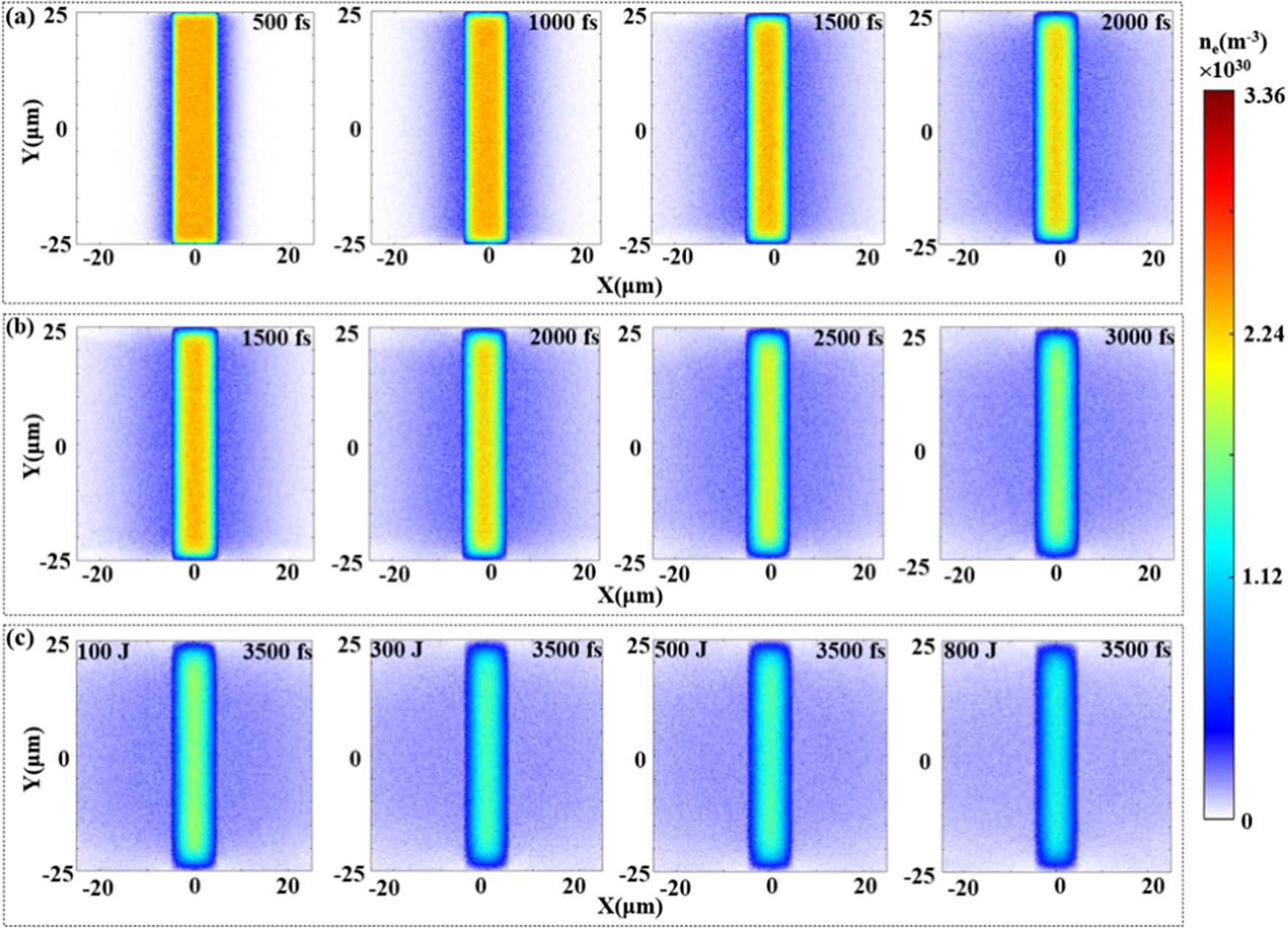
Firstly, the influence of laser energy on the escaping electrons during laser–target interaction is simulated. Here, the PIC simulations were conducted using EPOCH code^[ Reference Arber, Bennett, Brady, Lawrence-Douglas, Ramsay, Sircombe, Gillies, Evans, Schmitz, Bell and Ridgers^27, Reference Wang, Yan, Cui, Xu, Zhang, Qi, He, Zhang, Li, Deng and Zhou^28]. The simulations were carried out on Au film targets uniformly configured with 10-μm thickness and 50-μm width, as shown in Figure 2. In the simulation setup, the left-hand boundary of the domain serves as the laser injection boundary. A monitoring plane is placed 5 μm away from the target on the right-hand side to record the escaping electrons. All boundaries are assumed to open boundaries for particle outflow. In Figure 2(a), the laser parameters are set to an energy of 100 J, a pulse width of 1 ps and a focal power density of 8 × 10¹⁸ W/cm², and they are 800 J, 2 ps and 1.3 × 10¹⁹ W/cm² in Figure 2(b). In Figure 2(c), the pulse width is fixed at 2 ps for all cases and the laser energies are adjusted to 100, 300, 500 and 800 J. All the aforementioned laser pulses are incident perpendicularly onto the target surface. The pulsed lasers (100 J, 1 ps, focal power density: 8 × 10¹⁸ W/cm²) produce escaped hot electrons with a maximum energy of 52 MeV, which is enhanced to 57 MeV by strengthening the laser energy to 800 J (focal power density: 1.3 × 10¹⁹ W/cm²). Figure 2(c) shows that the hot electrons are significantly increased with laser energy from 100 to 800 J, while maintaining a fixed pulse duration and focal spot dimensions. The energy spectra of the escaping electrons created by the four laser energies are given in Figure 1 in the Supplementary Material. Consequently, the increased population of escaping electrons enhances the peak target holder current I _e, which is proportional to the charge deficit on the target Q _e^[ Reference Consoli, Tikhonchuk, Bardon, Bradford, Carroll, Cikhardt, Cipriani, Clarke, Cowan, Danson, Angelis, Marco, Dubois, Etchessahar, Garcia, Hillier, Honsa, Jiang, Kmetik, Krása, Li, Lubrano, McKenna, Metzkes-Ng, Poyé, Ra̧czka, Prencipe, Smith, Vrana, Woolsey, Zemaityte, Zhang, Zhang, Zielbauer and Neely^2, Reference Poyé, Hulin, Bailly-Grandvaux, Dubois, Ribolzi, Raffestin, Bardon, Lubrano-Lavaderci, D'Humières, Santosl, Nicolaï and Tikhonchuk^11], leading to emission of intense EMPs based on Equations (1)–(5).

Figure 2

Results of PIC simulations. (a) Electron distribution evolution under the 8 × 10¹⁸ W/cm² laser condition. (b) Electron distribution evolution under the 1.3 × 10¹⁹ W/cm² laser condition. (c) Comparison of electron distribution under four energy conditions.

Figure 2 Long description

The matrix contains three labeled rows, each with four panels. Row one, labeled a, shows electron density maps at 500, 1000, 1500, and 2000 femtoseconds for 8 times 10 super 18 watts per square centimeter. Row two, labeled b, shows maps at 1500, 2000, 2500, and 3000 femtoseconds for 1.3 times 10 super 19 watts per square centimeter. Row three, labeled c, compares four energy conditions at 3500 femtoseconds: 100 joules, 300 joules, 500 joules, and 800 joules. Each panel plots X in micrometers on the horizontal axis and Y in micrometers on the vertical axis, ranging from negative 25 to 25. Electron density, n sub e in units of meters to the negative three, is indicated by a vertical color bar at the far right, spanning from 0 in blue to 3.36 times 10 super 30 in red. In all panels, a central vertical band shows the highest density, which decreases outward. In row a and b, the density band remains prominent but gradually diffuses over time. In row c, increasing energy results in a broader, less intense central band. The color transitions from red and yellow at early times or lower energies to blue at later times or higher energies, indicating density reduction and spatial broadening.

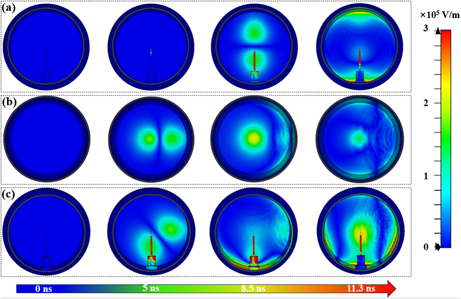
To distinguish the two sources for EMP radiation, a 3D electromagnetic model is subsequently established to reveal the EMP intensity and distributions. The time-domain solver in CST Studio Suite employs finite integration techniques to directly solve Maxwell’s equations in the time domain, iteratively computing the evolution of electromagnetic fields over time. The simulation geometrical structure is illustrated in Figure 2 in the Supplementary Material. The model is built as a spherical target chamber with an inner radius of 1250 mm and a thickness of 50 mm, and target holders (F is the diameter and L is the length) are abstracted as cylindrical in multiple sections from the interior of the target chamber pointing to the target in the following order (F, L) = (340, 225), (240, 290), (50, 590), (10, 95) and (3, 50), in which the units are all in mm. The target chamber brace plate is a discus-like shape with a thickness of 20 mm and a radius of 1080 mm. A gold target with length and width of 6 mm and a thickness of 10 μm is added to the top of the target holder. Figure 3 displays the spatial-temporal evolution of EMPs generated by an escaping electron beam of the average energy: 12 MeV, 200 nC. Figure 3(a) shows that the EMP radiated from the target holder current by excluding the effects of electrons reaches approximately 200 kV/m, and it attains approximately 800 kV/m solely by escaping electrons in the absence of a target holder, as shown in Figure 3(b). Furthermore, the EMP is increased to approximately 1.7 MV/m due to spatial superposition by unifying the two sources, as displayed in Figure 3(c). The temporal evolution of electric field intensity is presented in Figure 3 in the Supplementary Material, suggesting that the produced EMPs are remarkably enhanced with the increase of escaped electrons. The electron trajectory is detailed in Figure 4 in the Supplementary Material. Comparative analysis reveals that the electrons induce imbalance of potential between the target and ground, thereby driving neutralization currents in the target holder for EMP generation, consistent with the proposed generation mechanisms^[ Reference Consoli, Tikhonchuk, Bardon, Bradford, Carroll, Cikhardt, Cipriani, Clarke, Cowan, Danson, Angelis, Marco, Dubois, Etchessahar, Garcia, Hillier, Honsa, Jiang, Kmetik, Krása, Li, Lubrano, McKenna, Metzkes-Ng, Poyé, Ra̧czka, Prencipe, Smith, Vrana, Woolsey, Zemaityte, Zhang, Zhang, Zielbauer and Neely^2, Reference Poyé, Hulin, Bailly-Grandvaux, Dubois, Ribolzi, Raffestin, Bardon, Lubrano-Lavaderci, D'Humières, Santosl, Nicolaï and Tikhonchuk^11].

Figure 3

Results of three-dimensional electromagnetic field simulations. (a) EMP distribution under the target holder current radiation model. (b) EMP distribution generated by escaping electrons only. (c) Combined EMP distribution from both escaping electrons and target holder neutralization currents.

Figure 3 Long description

There are three rows labeled a, b, and c, each with four circular panels arranged from left to right, representing time points 0 nanoseconds, 5 nanoseconds, 8.5 nanoseconds, and 11.3 nanoseconds. The color scale bar on the right ranges from blue at zero to red at three times ten to the five volts per meter. Row a shows the target holder current radiation model: the first panel is uniformly blue, the second shows a faint vertical feature at the bottom center, the third displays a central green region, and the fourth has a yellow-green area spreading upward from the bottom. Row b shows the escaping electrons only: the first panel is blue, the second has two green spots near the center, the third shows a central yellow-green region, and the fourth displays a diffuse green area. Row c shows the combined model: the first panel is blue, the second has a vertical feature at the bottom center, the third shows a green region at the bottom center, and the fourth displays a strong yellow region extending upward. The time progression is indicated by a horizontal color bar at the bottom, ranging from blue at zero nanoseconds to red at eleven point three nanoseconds.

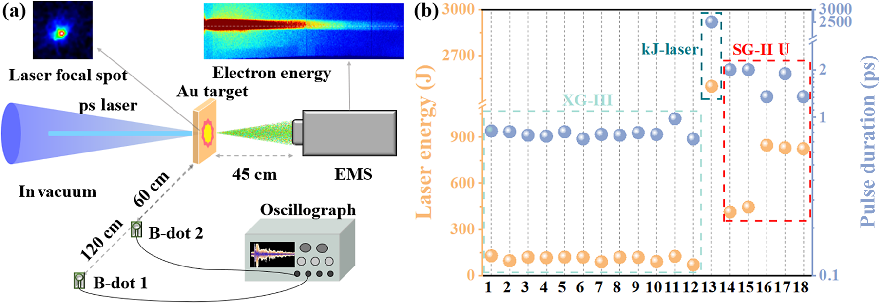
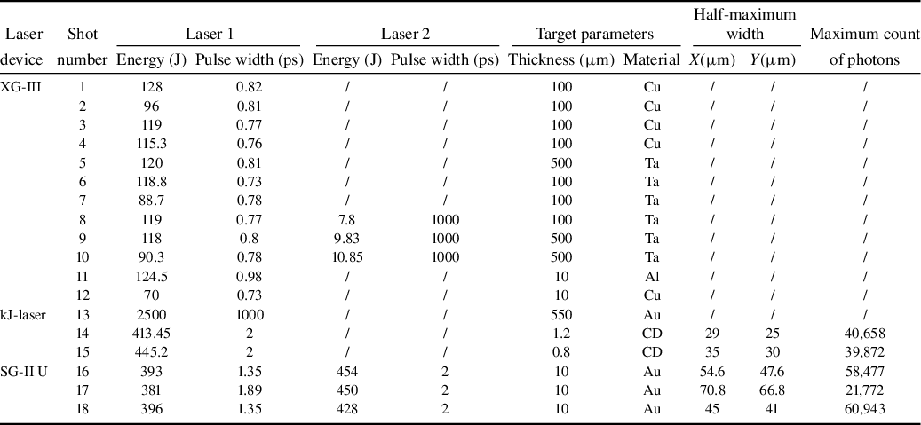
The simulation results demonstrate that increasing the laser focal power density boosts electron emission, which in turn amplifies the resulting EMPs. Specifically, based on the PIC simulation results in Figure 2, a higher laser focal power density corresponds to a smaller number of residual electrons in the same target, indicating a larger quantity and higher energy of escaping electrons. Meanwhile, the 3D electromagnetic field simulation results in Figure 3 as well as Figure 5 in the Supplementary Material demonstrate that a greater number and higher energy of escaping electrons drive a larger target holder current, which subsequently radiates more intense EMPs through the half-wave dipole antenna model. Based on the above theoretical framework, a series of experiments are designed to validate the proposed model. All experimental EMP measurements were performed at the SG-II U picosecond petawatt laser facility and XG-III laser facility in the Science and Technology on Plasma Physics Laboratory. Figure 4(a) shows the experimental layout of the SG-II U picosecond petawatt laser facility; under zero-delay conditions, dual-picosecond laser pulses are focused onto a 10-μm-thick planar gold target. The energy and pulse duration parameters for the dual laser pulses are provided for shots 16–18 in Figure 4(b) and Table 1. A B-dot probe (effective bandwidth: 0.1–3 GHz) is positioned 60 cm away from the target to record the EMP amplitude. The probe is connected with an oscilloscope (Tektronix DPO 70604C with a 6 GHz analog bandwidth and a 25 GS s^–1 sampling rate) via the shielded cables to measure EMP signals. The connecting cables used are RG223 feedlines, featuring an impedance of 50 Ω and a cutoff frequency of 31 GHz, with a total length of 20 m, and the cables are wrapped in copper foil for electromagnetic shielding. The attenuation of the cable is 13 dB per 100 m at 100 MHz.

Figure 4

Experimental arrangements. (a) Schematic diagram of the experimental layout. (b) Laser parameters for each shot in this experiment.

Figure 4 Long description

Panel a, at left, is a schematic diagram. At the leftmost edge, a blue cone labeled ps Laser points rightward toward a yellow square labeled Au target. Above the cone is an inset showing a colored laser focal spot. The Au target is 60 cm from the laser source and 45 cm from a gray box labeled E M S, with green arrows indicating electron energy measurement. Two B-dot detectors are shown below the target, labeled B-dot 1 at 120 cm and B-dot 2 at 60 cm from the target, both connected to an Oscillograph at the bottom right. Panel b, at right, is a scatter plot with the x-axis labeled 1 to 18, representing shot numbers. The left y-axis is labeled Laser energy (J) from 0 to 3000 in orange, and the right y-axis is Laser pulse (ps) from 0.1 to 3 in blue. Blue and orange circles represent pulse duration and energy for each shot. Shots 1 to 12 are grouped under X G dash I I I, shots 13 to 18 under S G dash I I U P, with higher energy and pulse values in the latter group. Dashed boxes highlight these groupings. All text and values are transcribed as shown.

Table 1

Laser parameters and target parameters for each shot in this experiment.

Table 1 Long description

The table contains 18 rows and 11 columns. The first column lists laser devices: X G dash I I I, K J dash laser, and S G dash I I U. The second column shows shot numbers from 1 to 18. Columns three to six detail Laser 1 and Laser 2 parameters: energy in joules and pulse width in picoseconds, with some entries marked as forward slash for missing data. Columns seven and eight specify target thickness in micrometers and material, including C u, T a, A l, A u, and C D. Columns nine and ten provide half-maximum widths in micrometers for X and Y, with values present only for shots 14 to 18. The final column lists maximum photon counts, populated for shots 14 to 18 with values such as 40,658, 39,872, 58,477, 21,772, and 60,943. The table structure groups shots by device, with X G dash I I I covering shots 1 to 12, K J dash laser for shot 13, and S G dash I I U for shots 14 to 18. Data is organized to compare laser and target parameters across devices and shots.

The electron spectrometer with a deflecting magnetic field of 2000 G is placed 45 cm in front of the target for monitoring the ejected electrons. Moreover, an image plate (IP) is used to grasp the deflection distance of electrons, which can quantify electrons with different energies. The focal spot size is recorded by a pinhole camera (the recorded focal spot information during the dual-picosecond laser pulses is presented in Figure 6 in the Supplementary Material). The pinhole camera utilizes a tantalum (Ta) pinhole plate with a thickness of 20 μm and a diameter of 7 mm. The pinhole sizes range from 8 to 15 μm and the pixel size of the pinhole camera is 13.5 μm.

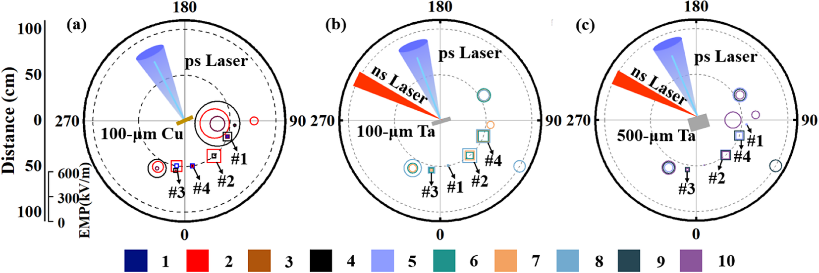
In Figure 5, the left-hand scale indicates the distance within the laser target chamber, with the outermost black circle representing the chamber wall. The coordinate ‘0’ corresponds to the exact center of the chamber, and the radius of the XG-III chamber is 1.1 m. The results in Figures 5(a)–5(c) are all obtained from EMP measurements inside the XG-III chamber with different target parameters. The targets are placed at the exact center of the chamber, and their thicknesses and materials are marked in all figures. Both picosecond and nanosecond laser pulses irradiate the target surface and generate EMPs. Apart from the target and laser, the remaining graphics represent EMP measurement results: the center of each graphic indicates the position of the EMP probe (antenna), while the size of the graphic (corresponding to the diameter of the circular marker or the side length of the square marker) refers to the EMP intensity with the intensity scale located in the lower-left corner of Figure 5. The various colors correspond to different experimental shots with the color-code mapping indicated by the colored squares below the figure. The corresponding laser and target parameters for each shot can be found in Figure 4(b) and Table 1. In addition, the graphics are indicated by two shapes: circles represent signals obtained with a naked antenna, while squares represent signals measured in a shielded box with specific shields labeled as #1–#4. Shielding device #1 is composed of double-layer aluminum with a thickness of 3 mm; #2 represents an open configuration; #3 consists a shielding box with a front panel of lead-glass (50 mm thickness) and the other sides are made of 3 mm aluminum; #4 is a shielding box with a front panel of polytetrafluoroethylene (5 mm thick) and the remaining five components are also 3 mm-thick aluminum. The schematic diagrams of the above shielding boxes are presented in Figure 7 in the Supplementary Material. During shots 3 and 4, shielding devices #1 and #4 are swapped in position.

Figure 5

Experimental results at the XG-III laser facility. Distribution of EMPs generated from (a) the 100-μm-thick Cu flat target, (b) the 100-μm-thick Ta flat target and (c) the 500-μm-thick Ta flat target.

Figure 5 Long description

From left to right, panel a shows a 100-micrometer Cu target with EMP values marked by colored circles and squares, concentrated between 0 and 90 degrees, with the highest EMP near the center. The ps Laser region is shaded blue, and four detector positions are labeled numerically. Panel b displays a 100-micrometer Ta target, with EMPs distributed more broadly, lower in intensity, and detector positions similarly labeled. The ps Laser region is again shaded blue. Panel c presents a 500-micrometer Ta target, with EMPs shown as purple circles and squares, distributed even more widely, and the ns Laser region shaded red. All panels use a radial axis for distance in centimeters and a vertical axis for EMP in kilovolts per meter. The legend below assigns colors to ten EMP events or detectors.

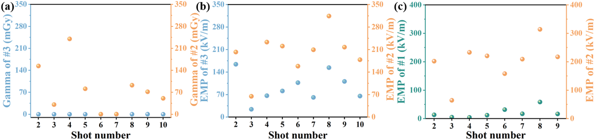
The data in Figure 5(a) are derived from a preparatory experiment, where the shot-to-shot variation in intensity is mainly due to laser fluctuations^[ Reference Xia, Zhang, Cai, Xu, Wang, Zhou, Tian, Zhang, Liu, Yi, Li and Zhu^21], but the changing tendency can be still reasonably revealed. The comparison of the EMP spatial distribution in the figure reveals that the distribution within the target chamber is relatively complex. Overall, the intensity generally decreases with increasing distance from the source; however, an enhancement is observed near the chamber walls. This phenomenon is attributed to EMP reflections^[ Reference He, Deng, Zhang, Xia, Zhang, Meng, He, Huang, Yang, Liu, Fan, Lin, Zhou, Li and Yan^29] and the deposition of charged particles on the chamber walls^[ Reference Consoli, Andreoli, Cipriani, Cristofari, De Angelis, Di Giorgio, Duvillaret, Krása, Neely, Salvadori, Scisciò, Smith and Tikhonchuk^30]. The EMP intensity behind the target is higher than that at the sides, as shown in Figure 5(a), point #2 in the figure behind the target, with an intensity of 221 kV/m at a distance of 50 cm from the target spot. EMPs measured by the naked antennas at other positions on the target side are 350, 149 and 111 kV/m, corresponding to distances of 30, 58 and 76 cm, respectively. After distance normalization to 50 cm, the EMP intensities are converted to 210, 173 and 169 kV/m. Therefore, the higher EMP intensity behind the target is confirmed compared to those on the target side, consistent with the EMP generation model mentioned earlier in Figure 3(c). Besides the half-wave dipole antenna model, the motion of charged particles in space also contributes to EMP generation. Since fewer escaping electrons are distributed at the target sides^[ Reference Chen, Sheng and Zhang^31– Reference Sheng, Sentoku, Mima, Zhang, Yu and Meyer-ter-Vehn^33], the EMP intensity behind the target is higher than at the sides. For Ta targets with thicknesses of 100 and 500 μm, when the laser reaches stable conditions, the produced EMPs exhibit strong stability. In addition, the EMP intensity shows an increasing trend after a ns pre-pulse is added. The ns pulse makes it possible to generate a surface plasma that more efficiently absorbs the ps laser pulse by overcoming only the work function of Ta, which is around 4.1 eV, promoting the generation of higher-intensity EMPs. Figures 14 and 15 in the Supplementary Material present EMP intensities generated from100- and 500-μm-thick Ta targets with and without a ns laser. To compare the shielding performance of different shielding devices, gamma-ray dosimeters were placed inside the shielding devices in addition to the EMP probes to record gamma radiation intensity. The shielding performance comparisons are shown in Figure 6. Specifically, Figures 6(a) and 6(b) compare the EMP intensity and gamma radiation dose in #3 and #2, respectively, while Figure 6(c) compares the EMP intensity between #1 and #2.

Figure 6

Extended experimental results at two different conditions. (a) The dose rates of gamma radiation in #3 and #2. (b) The EMP intensity in #3 and #2. (c) The EMP intensity in #1 and #2.

Figure 6 Long description

Panel a on the left plots shot number from two to ten on the x-axis. The left y-axis shows Gamma of number three in m G y from zero to three hundred fifty, and the right y-axis shows Gamma of number two in m G y from zero to three hundred fifty. Orange points (number two) are consistently higher than blue points (number three), with both peaking at shot three and declining. Panel b in the center plots shot number from two to ten. The left y-axis is E M P of number three in k V per meter from zero to three hundred fifty, and the right y-axis is E M P of number two in k V per meter from zero to three hundred fifty. Orange points (number two) are higher than blue points (number three), with both showing a peak at shot three and a general decline. Panel c on the right plots shot number from two to nine. The left y-axis is E M P of number one in k V per meter from zero to four hundred, and the right y-axis is E M P of number two in k V per meter from zero to four hundred. Orange points (number two) are higher than green points (number one), with both showing a peak at shot three and a gradual decrease. All panels use dual y-axes to compare two datasets per panel, with consistent trends of higher values for number two and peak responses at shot three.

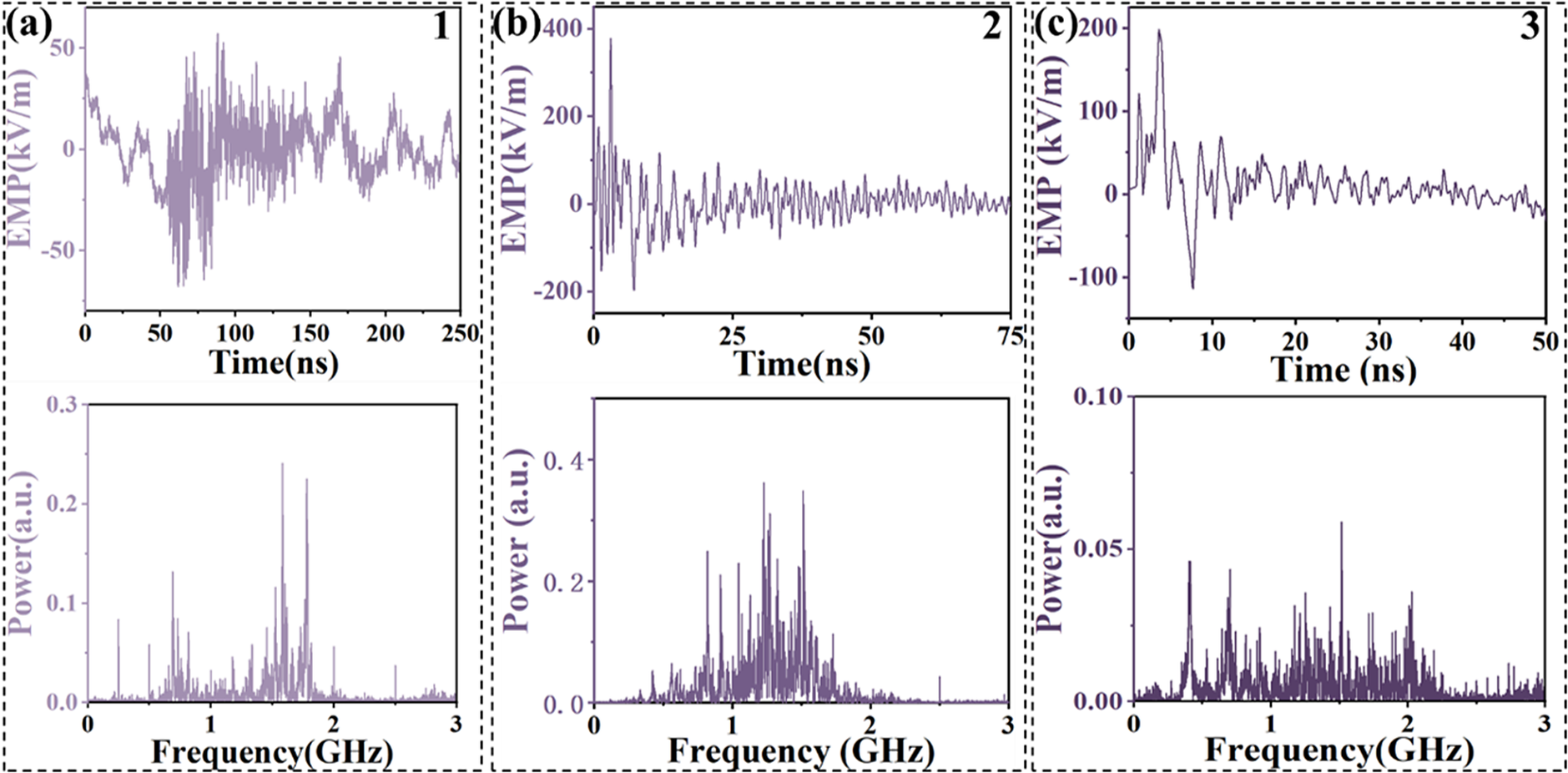
As shown in Figures 5 and 6(c), the double-layer aluminum shielding box exhibits superior attenuation of EMP intensity compared to the other three shielding devices. This is attributed to the presence of system generated EMPs^[ Reference Consoli, Tikhonchuk, Bardon, Bradford, Carroll, Cikhardt, Cipriani, Clarke, Cowan, Danson, Angelis, Marco, Dubois, Etchessahar, Garcia, Hillier, Honsa, Jiang, Kmetik, Krása, Li, Lubrano, McKenna, Metzkes-Ng, Poyé, Ra̧czka, Prencipe, Smith, Vrana, Woolsey, Zemaityte, Zhang, Zhang, Zielbauer and Neely^2, Reference Zhang, Meng, Xu, Wu, Zhong and Feng^34, Reference Chen, Li, Zhou, Deng and Zeng^35] (SGEMPs, generated by high-energy particle interactions with matter) within the shielding box. The inner layer of the double-layer shielding box provides additional suppression of SGEMPs, achieving an average attenuation performance exceeding 20 dB across multiple shots. A comparison between Figures 6(a) and 6(b) indicates that shielding device #3 effectively attenuates internal gamma radiation to near-zero levels (approximately 0 mGy; the gamma-ray energy range of the XG-III laser facility is approximately 50–200 keV). However, it still permits a certain intensity of EMPs to penetrate the shielding enclosure (the EMP intensity is reduced by approximately half compared to that in the unshielded environment). This selective shielding capability enables partial isolation of the complex radiation environment within the target chamber, thereby providing a foundation for investigating device radiation damage under controlled, single-radiation conditions in high-power laser facilities. Meanwhile, the results presented in Figure 6(c) offer a novel approach for radiation protection of equipment within high-power laser target chambers. The EMP waveforms and frequency spectral distributions with the highest intensities of shots 1–3 are as shown in Figure 7. Figure 7 shows that, under the low-energy single-picosecond laser configuration and the short target holder structure of the XG-III laser facility, the generated EMP intensity is only of the order of hundreds of kV/m, with the frequency range primarily concentrated between 500 MHz and 2 GHz; the other EMP waveforms and frequency spectral distributions^[ Reference Consoli, Tikhonchuk, Bardon, Bradford, Carroll, Cikhardt, Cipriani, Clarke, Cowan, Danson, Angelis, Marco, Dubois, Etchessahar, Garcia, Hillier, Honsa, Jiang, Kmetik, Krása, Li, Lubrano, McKenna, Metzkes-Ng, Poyé, Ra̧czka, Prencipe, Smith, Vrana, Woolsey, Zemaityte, Zhang, Zhang, Zielbauer and Neely^2, Reference He, Deng, Meng, Zhang, Cui, Qi, Yang, Liu, Fan, Wang, Yi, Gu, Lin, Consoli, Zhou and Li^17] with the highest intensities across all shots in Figure 5 are provided in the Supplementary Material, and we also add the PIC simulation results for a tantalum target of 100 μm thickness, as shown in Figure 8 in the Supplementary Material, which indicate that the majority of electrons remain confined within the target due to its thickness. In addition to the aforementioned target configurations, experiments using 10-μm-thick copper targets and 10-μm-thick aluminum targets were conducted on the XG-III facility. EMPs with field strengths of approximately 200 kV/m were measured along the target rear normal direction at approximately 40 cm for both target types. The corresponding EMP waveforms and frequency spectra are shown in Figure 12 in the Supplementary Material.

Figure 7

Time-domain and frequency-domain results of electromagnetic pulses from the XG-III laser facility: (a) shot 1; (b) shot 2; (c) shot 3.

Figure 7 Long description

The multiplot consists of three columns labeled a, b, and c, each representing shot 1, shot 2, and shot 3, respectively. The top row displays line graphs of E M P in kilovolt per meter versus Time in nanoseconds. Shot 1 shows a fluctuating E M P signal from minus 100 to plus 100 over 250 nanoseconds. Shot 2 shows a sharp initial peak near 200 kilovolt per meter, then decays toward zero over 75 nanoseconds. Shot 3 shows a rapid initial peak near 200 kilovolt per meter, then decays more quickly over 50 nanoseconds. The bottom row shows frequency-domain line graphs of Power in arbitrary units versus Frequency in gigahertz. Shot 1 has multiple sharp peaks between 0 and 3 gigahertz, with the highest near 0.5 gigahertz. Shot 2 shows higher overall power with pronounced peaks near 0.5 and 1.5 gigahertz. Shot 3 displays lower power with broader, less pronounced peaks across the spectrum. All axes are labeled and units are specified.

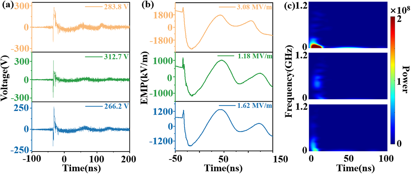
The interaction between dual-picosecond laser pulses (with near-zero temporal delay between the two lasers, as verified by overlapping focal spots that effectively represent a single higher-energy pulse) and 10-μm-thick gold target at the SG-II U picosecond petawatt laser facility produced EMP results as shown in Figure 8 (in the figure, the panels from bottom to top correspond to shot numbers 16–18, respectively). Figure 8(a) displays the voltage waveforms recorded by the oscilloscope (voltage peaks are shown in the upper right-hand corner), while Figure 8(b) presents the derived electric field strength waveforms (electric field peaks are shown in the upper right-hand corner). The electric field strength is derived from the voltage by the following formula^[ Reference Xia, Zhang, Cai, Xu, Wang, Zhou, Tian, Zhang, Liu, Yi, Li and Zhu^21]:

(6) $$\begin{align}V(t)=-\frac{\mathrm{d}\Phi (t)}{\mathrm{d} t}=-A\frac{\mathrm{d} B(t)}{\mathrm{d} t},\end{align}$$

(7) $$\begin{align}{\int}_0^{\tau }V(t) \mathrm{d}t=-A{\int}_0^{\tau}\frac{\mathrm{d}B(t)}{\mathrm{d}t} \mathrm{d}t,\end{align}$$

(8) $$\begin{align}B(t)=-\frac{1}{A}{\int}_0^{\tau }V(t) \mathrm{d}t,\end{align}$$

(9) $$\begin{align}E\approx cB=-\frac{c}{A}{\int}_0^{\tau }V(t) \mathrm{d}t.\end{align}$$

Figure 8

Experimental results at the SG-II U picosecond petawatt laser facility. (a) Voltage intensity waveforms. (b) Electric field strength waveforms. (c) EMP spectral distribution.

Figure 8 Long description

There are three panels arranged left to right. The left panel shows three line graphs of voltage in volts versus time in nanoseconds, with traces in orange, green, and blue, labeled 283.8 V, 312.7 V, and 266.2 V. The middle panel displays three line graphs of E M P in kilovolts per meter versus time in nanoseconds, with traces in orange, green, and blue, labeled 3.08 M V per meter, 1.18 M V per meter, and 1.62 M V per meter. The right panel contains three vertically stacked heatmaps of frequency in gigahertz versus time in nanoseconds, with a color bar on the right indicating power from zero to two times ten to the eight. The highest power is concentrated at low frequencies and early times in the top heatmap.

Here, V denotes the voltage amplitude, Φ(t) represents the time-dependent magnetic flux, A is the equivalent area of the antenna (78.5 mm²), B(t) corresponds to the magnetic strength and c signifies the speed of light. Figure 8(c) illustrates the frequency spectral distribution of the EMP signals.

Figure 8(a) demonstrates prolonged voltage oscillations lasting more than 200 ns, significantly exceeding the EMP duration (~100 ns) generated by laser–planar target interactions in the XG-III facility. According to Equation (9), this extended integration time results in enhanced EMP intensity. In Figure 8(b), three consecutive dual-picosecond laser shots produced EMPs with intensities exceeding 1 MV/m, achieving a peak field strength of 3.08 MV/m (shot 18); the intensity is nearly four times that of the EMP radiation generated by the interaction of a single-picosecond laser shot from the SG-II U picosecond petawatt laser facility with a 1.2-μm-thick CD target (shot 14). The observed intensity variations among the three shots arise from differences in laser focal power density. Despite comparable laser energy and pulse duration, the focal spot sizes differ significantly across the experiments (as shown in Figure 6 in the Supplementary Material). Since laser focal power density exhibits an inverse square dependence on the focal radius (P∝1/r ²), this geometric scaling law directly amplifies EMP intensity disparities, with the smallest focal radius configuration (shot 18) generating EMP fields 2.6 times stronger than the largest spot case (shot 17). The dashed lines highlight the temporal delay (~3 ns) between the initial rise and the first peak amplitude of the EMPs, consistent with the evolutionary timescale observed in 3D electromagnetic field simulations (Figure 2(c)). The three EMP waveforms exhibit similar profiles, with subsequent oscillations attributed to reflections within the target chamber and oscillations of the target holder current (see Figures 3 and 5 in the Supplementary Material). Figure 8(c) reveals that the EMP spectrum is primarily concentrated in the hundreds of MHz region. Based on the radiation characteristics of the half-wave dipole antenna model, the EMP frequency can be calculated as follows^[ Reference Poyé, Hulin, Bailly-Grandvaux, Dubois, Ribolzi, Raffestin, Bardon, Lubrano-Lavaderci, D'Humières, Santosl, Nicolaï and Tikhonchuk^11, Reference He, Kang, Ren, Tian, Wang, Zhang, Liu, Yang, Liu, Sun, Zhu, Zhou and Li^12, Reference He, Deng, Meng, Zhang, Cui, Qi, Yang, Liu, Fan, Wang, Yi, Gu, Lin, Consoli, Zhou and Li^17, Reference Xia, Zhang, Cai, Xu, Wang, Zhou, Tian, Zhang, Liu, Yi, Li and Zhu^21]:

(10) $$\begin{align}f\cong \frac{c}{4l},\end{align}$$

where f represents the EMP frequency, l the target holder length (∼1 m) and c the speed of light. This indicates that the frequency of the electromagnetic waves radiated by the half-wave dipole antenna model approximates to hundreds of MHz, aligning with the spectral results in Figure 8(c) (the power shown in the figure represents the signal power absorbed by the antenna). As shown in Figures 10–13 in the Supplementary Material, the EMP spectrum in the XG-III facility is predominantly distributed from hundreds of MHz to 2 GHz. This distribution arises from the shorter target holder length (5–26 cm)^[ Reference He, Deng, Meng, Zhang, Cui, Qi, Yang, Liu, Fan, Wang, Yi, Gu, Lin, Consoli, Zhou and Li^17, Reference Xia, Zhang, Cai, Xu, Wang, Zhou, Tian, Zhang, Liu, Yi, Li and Zhu^21] in the facility, which, according to the half-wave dipole antenna model, results in higher EMP frequencies. Furthermore, due to variations of laser parameters, the XG-III facility drives the escaped electrons with lower charge quantities and induces weaker target holder current intensities. Consequently, the EMPs generated by escaping electrons within the target chamber also contribute to the overall spectral characteristics^[ Reference He, Deng, Meng, Zhang, Cui, Qi, Yang, Liu, Fan, Wang, Yi, Gu, Lin, Consoli, Zhou and Li^17, Reference Xia, Zhang, Cai, Xu, Wang, Zhou, Tian, Zhang, Liu, Yi, Li and Zhu^21].

Figure 9

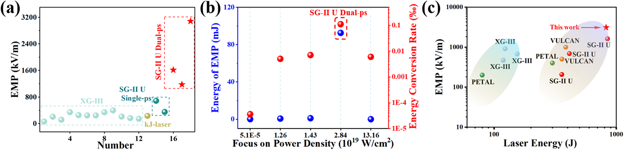
The peak EMP intensity. (a) The EMP intensity in this experiment. (b) The EMP energy and energy conversion rate. (c) Comparison of EMP intensity of ps laser facilities.

Figure 9 Long description

Panel a, at left, plots E M P in kilovolt per meter on the y-axis versus Number on the x-axis. Data points cluster at low E M P for X G-III, S G-II U P Single-ps, and kJ-laser, while S G-II U P Dual-ps, marked with red stars, shows a sharp increase above 1600 up to 3200 kilovolt per meter. Panel b, center, has Energy of E M P in millijoule on the left y-axis, Energy Conversion Rate percent on the right y-axis, and Focus on Power Density in 10 to the 19 watt per centimeter squared on the x-axis. Blue circles show E M P energy rising with power density, while red circles show conversion rate, with S G-II U P Dual-ps highlighted at the highest values. Panel c, right, plots E M P in kilovolt per meter versus Laser Energy in joule, both axes on logarithmic scales. Clusters for X G-III and PETAL are at lower left, S G-II U P and VULCAN at mid to upper right, and ‘This work’ (S G-II U P Dual-ps) is marked with a red star at the highest E M P and laser energy. Arrows and shaded regions group facilities for comparison.

In our prior research, simulations have confirmed that the chamber resonant frequency of the SG-II U picosecond petawatt laser facility corresponds to hundreds of MHz^[ Reference Niu, Kang, Xu, Xie, Teng, Liu, Sun and Li^24], closely aligned with the EMP frequency spectrum, and that the highly conductive chamber wall material facilitates electromagnetic wave reflection and oscillation within the target chamber^[ Reference Katsumata^36]; this also corresponds to the longer duration of the EMPs in this experiment. Figure 9 in the Supplementary Material presents electron spectral data recorded by the front-target spectrometer, demonstrating that the escaping electron charge is modulated by laser focal power density parameters. Specifically, the three laser shots have similar energy and pulse duration, but they exhibit significant differences in focal size. A smaller focal size corresponds to a higher laser focal power density, which in turn generates escaping electrons with larger charge and higher cutoff energy. The EMP intensity exhibits a positive correlation with the escaping electron charge, as the latter determines the neutralization current amplitude in the target holder system – a critical factor governing EMP generation, which can be validated by Equations (1)–(4) and (6).

In summary, the generation of MV/m-level EMPs can be attributed to the following mechanism: the simultaneous action of dual-picosecond laser pulses on a gold target significantly increases the on-target laser focal power density, which enhances power density and drives a large number of electrons to escape from the target, leading to more severe charge depletion within the target material. Consequently, a stronger neutralizing current is generated on the target holder, ultimately radiating a more intense EMP in the hundreds of MHz band via the half-wave dipole antenna model. This causal chain aligns well with the PIC simulation results (higher focal power density drives more electron escape), the 3D electromagnetic field simulation results (higher escaping electron charge yields stronger EMPs) and the theoretical calculations. The experimental data closely match the simulated results (Figures 3(c) as well as Figure 5 in the Supplementary Material), confirming the validity of the theoretical model.

Based on the aforementioned results, we performed a comparative analysis of EMP intensity, energy and laser-to-EMP energy conversion efficiency, as summarized in Figure 9. Figure 9(a) compares the EMP intensities across all experimental shots (refer to Figure 4(b) and Table 1), demonstrating that dual-ps laser pulses generate EMPs with field strengths significantly exceeding those of other configurations (all intensities have been distance normalized^[ Reference Niu, Kang, Xu, Xie, Teng, Liu, Sun and Li^24], and the normalization is carried out based on the inverse square relationship between EMP energy density and propagation distance). The EMPs generated by both the XG-III facility and the SG-II U picosecond petawatt laser facility under single-picosecond laser irradiation exhibit field strengths of the order of hundreds of kV/m, several times weaker than those produced by the dual-ps laser configuration at the SG-II U picosecond petawatt laser facility. This stark contrast in EMP intensities provides direct experimental validation of the theoretical model proposed in this work. The rise time (τ _r) and full width at half maximum (FWHM) (τ _FWHM) of EMPs are derived based on the classical double exponential pulse function B _D(t), as expressed by the following equation^[ Reference De Marco, Krása, Cikhardt, Velyhan, Pfeifer, Dudžák, Dostál, Krouský, Limpouch, Pisarczyk, Kalinowska, Chodukowski, Ullschmied, Giuffrida, Chatain, Perin and Margarone^37]:

(11) $$\begin{align}{B}_\mathrm{D}(t)={B}_0\left[\exp \left(-\frac{t}{\tau_{\mathrm{dis}}}\right)-\exp \left(-\frac{t}{\tau_{\mathrm{ch}}}\right)\right],\end{align}$$

where B ₀ is the B-field pulse amplitude and τ _dis and τ _ch are the discharge and charge coefficients, respectively, of EMP radiation. The dual-ps laser configuration generates EMPs with a rise time of approximately 15 ns and an FWHM of approximately 55 ns (shot 18); the rise time and FWHM of the EMP of the XG-III laser facility are about 3.3 and 8.7 ns, respectively (shot 3), while the SG-II U picosecond petawatt laser facility single-ps laser yields intermediate durations (rise time: 10.4 ns; FWHM: 19.1 ns; shot 14). The results above demonstrate that the EMP generated by the dual-ps laser exhibits a reduced high-frequency component and features such as an extended signal duration, which are consistent with the characteristics shown in Figure 8.

Figure 9(b) contrasts the EMP energy and energy conversion rate under varying laser focal power densities. The results reveal that the dual-ps laser-driven EMP generation mechanism achieves further enhancements in both EMP energy and laser-to-EMP conversion efficiency. The Poynting vector S = E × H is used to calculate the EMP energy (E _EMP) absorbed by the B-dot antenna (where E is the EMP electric field strength and H is the EMP magnetic field strength)^[ Reference Kugland, Aurand, Brown, Constantin, Everson, Glenzer, Schaeffer, Tauschwitz and Niemann^38]:

(12) $$\begin{align}{E}_{\mathrm{EMP}}=\sum S(t) A\varDelta t.\end{align}$$

Here, Δt denotes the EMP duration. The EMP energy for shot 18 can be calculated as 92.46 mJ, corresponding to a laser-to-EMP energy conversion rate of 0.11‰. Figure 9(c) compares EMP intensities generated by ps laser facilities, including the XG-III^[ Reference Xie, Wang, Li, Deng, Teng, Zhang, Tian, Wu, Gu, Zhou and Li^39], PETAL^[ Reference Bardon, Etchessahar, Lubrano, Bazzoli, Ferri, Ribolzi, Mirabel, La Fontaine and Mallejac^40], VULCAN^[ Reference Bradford, Woolsey, Scott, Liao, Liu, Zhang, Zhu, Armstrong, Astbury, Brenner, Brummitt, Consoli, East, Gray, Haddock, Huggard, Jones, Montgomery, Musgrave, Oliveira, Rusby, Spindloe, Summers, Zemaityte, Zhang, Li, McKenna and Neely^1, Reference Consoli, De Angelis, Robinson, Giltrap, Hicks, Ditter, Ettlinger, Najmudin, Notley and Smith^22] and SG-II U picosecond petawatt laser facilities. The results demonstrate that the EMP intensities generated in this study exceed those reported at other picosecond laser facilities.