


1 Introduction: why the electromagnetic pulses are so important
Generation of electromagnetic waves was first demonstrated by Heinrich Hertz in 1887 and since then has become a leading subject of research, with an enormous range of applications covering radio communications, electronics, computing, radar technology and multi-wavelength astronomy. The accessible spectrum of electromagnetic emissions continuously extends toward shorter waves from radio waves to microwaves, to optical and X-rays[Reference Carillon, Chen, Dhez, Dwivedi, Jacoby, Jaegle, Jamelot, Zhang, Key, Kidd, Klisnick, Kodama, Krishnan, Lewis, Neely, Norreys, Neill, Pert, Ramsden, Raucourt, Tallents and Uhomoibhi1], challenging now the gamma-ray domain[Reference Ledingham, Spencer, McCanny, Singhal, Santala, Clark, Watts, Beg, Zepf, Krushelnick, Tatarakis, Dangor, Norreys, Allott, Neely, Clarke, Machacek, Wark, Cresswell, Sanderson and Magill2]. It is also well recognized that strong electromagnetic waves could be dangerous for health and electronics. Methods of detection of electromagnetic waves and mitigation of their undesirable effects are also in full development[Reference Taylor3–Reference Buccheri, Huang and Zhang6].
Our review does not aim to cover all the issues related with the development and applications of pulsed electromagnetic sources. We address here the particular problem of microwaves generated during the interaction of powerful laser pulses with solid targets, in the domain extending from radiofrequencies (MHz) to terahertz. These electromagnetic pulses (EMPs), which are regularly detected in laser–target interactions with laser pulses from the femtosecond to the nanosecond range, are recognized as a threat to electronics and computers, and have stimulated the development of various protective measures. This situation has, however, significantly evolved since the invention of chirped pulse amplification (CPA) in lasers[Reference Strickland and Mourou7] and the rapid development of powerful sub-picosecond (sub-ps) laser systems[Reference Danson, Hillier, Hopps and Neely8]. Paradoxically, the interaction of sub-ps laser pulses with solid targets generates much stronger EMPs in the GHz domain than for nanosecond pulses of comparable energy. This fact has been reported in several publications during the past 15 years[Reference Mead, Neely, Gauoin, Heathcote and Patel9–Reference Eder, Anderson, Bailey, Bell, Benson, Bertozzi, Bittle, Bradley, Brown, Clancy, Chen, Chevalier, Combis, Dauffy, Debonnel, Eckart, Fisher, Geille, Glebov, Holder, Jadaud, Jones, Kaiser, Kalantar, Khater, Kimbrough, Koniges, Landen, MacGowan, Masters, MacPhee, Maddox, Meyers, Osher, Prasad, Raffestin, Raimbourg, Rekow, Sangster, Song, Stoeckl, Stowell, Teran, Throop, Tommasini, Vierne, White and Whitman12], but an understanding of the underlying physics has been attained only recently[Reference Dubois, Lubrano-Lavaderci, Raffestin, Ribolzi, Gazave, La Fontaine, d’Humières, Hulin, Nicolaï, Poyé and Tikhonchuk13].
The main source of strong GHz emissions has been identified as the return current flowing through the support structure to the target, charged by the intense laser–target interaction. Controlling the geometric and electrical characteristics of the target support has therefore become the major EMP mitigation approach. The understanding of the physics of EMP generation has substantially advanced very recently, and other mechanisms of EMP generation have been identified. Among the related main research topics, we mention: the excitation of chamber resonant modes; the characterization of secondary EMP sources; the scattered radiation. These processes are discussed in Sections 2.5 and 2.6 of this review. More accurate and efficient detection methods have been developed and used to deliver improved experimental data. At the same time, construction of a new generation of laser systems with pulse power exceeding the petawatt level[Reference Danson, Häfner, Bromage, Butcher, Chanteloup, Chowdhury, Galvanauskas, Gizzi, Hein, Hillier, Hopps, Kato, Khazanov, Kodama, Korn, Li, Li, Limpert, Ma, Nam, Neely, Papadopoulos, Penman, Qian, Rocca, Shaykin, Siders, Spindloe, Szatmari, Trines, Zhu, Zhu and Zuegel14] is opening the possibility of conducting experiments with high repetition rates, creating the need for more reliable and efficient EMP protection and mitigation techniques.
A full comprehension of the physics of EMP generation and the mechanisms of their operation will enable the creation of temporally and spatially controlled electromagnetic fields of high intensity and wide distribution. This would lead to the new and significant employment of laser–plasma interactions for powerful and versatile radiofrequency–microwave sources, which will be of direct interest to particle-acceleration schemes[Reference Wiedemann15–Reference Booske18], for which this is indeed of primary importance, as well as to a multidisciplinary range of applications: biological and medical studies of strong microwave interactions with cells[Reference Pakhomov, Miklavčič and Markov19]; medical engineering[Reference Schoenbach, Nuccitelli and Beebe20]; space communication[Reference Yoshida, Hasegawa and Kawasaki21]; plasma heating[Reference Kazakov, Ongena, Wright, Wukitch, Lerche, Mantsinen, Van Eester, Craciunescu, Kiptily, Lin, Nocente, Nabais, Nave, Baranov, Bielecki, Bilato, Bobkov, Crombé, Czarnecka, Faustin, Felton, Fitzgerald, Gallart, Giacomelli, Golfinopoulos, Hubbard, Jacquet, Johnson, Lennholm, Loarer, Porkolab, Sharapov, Valcarcel, Van Schoor and Weisen22]; material and device characterization[Reference Gupta and Gupta23–Reference Ott25]; EMP-radiation hardening of components[Reference Ott25]; and electromagnetic compatibility studies[Reference Ott25, Reference Degague and Hamelin26]. Understanding and controlling the sources of EMP radiation is also important for personnel protection[27].
This review paper summarizes the recent knowledge and experience gained by scientists working with high-power laser systems in many laboratories worldwide. Section 2 is dedicated to the theoretical understanding of the processes of electric charge accumulation on the target, return current formation and electromagnetic emission. Section 3 presents advancements in diagnostic techniques for the detection of EMPs, the experimental results obtained on different high-power laser facilities and their interpretation. Section 4 discusses the known techniques of mitigation of EMP effects, experience accumulated on several high-power laser facilities and possible applications of EMP. Finally, Section 5 concludes the review with a figure presenting the measured EMP levels on different laser facilities.
2 Physics of EMP generation
2.1 Target polarization
The principal source of electromagnetic emissions is charge separation and target polarization under the action of a laser pulse. Strong laser fields ionize the atoms and create a plasma, which expands from the target surface. As the laser pulse interacts essentially with electrons, the plasma is far from thermodynamic equilibrium. The electrons are heated and accelerated by the laser pulse and their average energy is much higher than that of ions. Moreover, a relatively small proportion of the electrons are accelerated to energies much above the average and may leave the target[Reference Rusby, Wilson, Gray, Dance, Butler, MacLellan, Scott, Bagnoud, Zielbauer, McKenna and Neely28], thus charging it positively. The total number of escaping electrons is defined by dynamical competition between the high energy of escaping electrons and the electric potential increase due to electron escape[Reference Rusby, Armstrong, Scott, King, McKenna and Neely29]. We describe numerical methods for the charge evaluation in Sections 2.3 and 2.4. Here, we present qualitative estimates for metallic targets irradiated with laser intensities  ${\sim}10^{18}{-}10^{20}~\text{W}\cdot \text{cm}^{-2}$. The characteristic electron energies are in the MeV domain and correspondingly the targets are charged to MV potentials in order to confine the remaining electrons[Reference Borghesi, Romagnani, Schiavi, Campbell, Haines, Willi, Mackinnon, Galimberti, Gizzi, Clarke and Hawkes30, Reference McKenna, Carroll, Clarke, Evans, Ledingham, Lindau, Lundh, McCanny, Neely, Robinson, Robson, Simpson, Wahlström and Zepf31].
The target potential  $\unicode[STIX]{x1D6F7}$ cannot be much larger than the characteristic energy (hot electron temperature) $T_{h}$ of laser heated electrons, $\unicode[STIX]{x1D6F7}\lesssim T_{h}/e$, where $e$ is the elementary charge. A more accurate relationship depends on the electron energy distribution, target material and other interaction characteristics. The hot electron temperature can be assimilated with a ponderomotive energy of electrons oscillating in the laser field[Reference Wilks, Kruer, Tabak and Langdon32],
 $$\begin{eqnarray}T_{h}\simeq (\unicode[STIX]{x1D6FE}_{0}-1)m_{e}c^{2},\end{eqnarray}$$
 where  $\unicode[STIX]{x1D6FE}_{0}=\sqrt{1+a_{0}^{2}/2}$ is the relativistic factor of an electron oscillating in the laser field, $a_{0}=eE_{0}/m_{e}\unicode[STIX]{x1D714}_{0}c$ is the dimensionless laser vector potential, $E_{0}$ is the laser electric field amplitude, $\unicode[STIX]{x1D714}_{0}$ is the laser frequency, $m_{e}$ is the electron mass and $c$ is the velocity of light. The formula for $\unicode[STIX]{x1D6FE}_{0}$ is written for a linearly polarized laser pulse. For circular polarization, $\unicode[STIX]{x1D6FE}_{0}=\sqrt{1+a_{0}^{2}}$.
In order to evaluate the charge accumulated on the target, the target capacity  $C_{t}$ must be known[Reference Raven, Rumsby, Stamper, Willi, Illingworth and Thareja33]. It can be approximated by the capacitance of a conducting disc of diameter $d_{t}$, $C_{t}\simeq 4\unicode[STIX]{x1D716}_{0}d_{t}$[Reference Jackson34], where $\unicode[STIX]{x1D716}_{0}$ is the vacuum dielectric permittivity. In our case, $d_{t}$ could be a transverse size of a metallic target or the size of the ionized zone accumulating the charge in a dielectric target. The capacitance of metallic targets of a centimeter size is of the order of 0.4 pF. As the maximum voltage is limited by the hot electron temperature, $\unicode[STIX]{x1D6F7}\lesssim T_{h}/e$, the maximum accumulated charge can be estimated as $Q_{e}\simeq C_{t}T_{h}/e$. The accumulated charge is also limited by the available laser pulse energy $E_{\text{las}}$, $Q_{e}\lesssim e\,\unicode[STIX]{x1D702}_{\text{las}}E_{\text{las}}/T_{h}$, with $\unicode[STIX]{x1D702}_{\text{las}}$ the laser conversion efficiency to hot electrons. Thus, the accumulated charge depends on both laser pulse energy and intensity. It is typically in the range from a few nC to a few $\unicode[STIX]{x03BC}\text{C}$ depending on the laser energy and focusing conditions[Reference Brown, Throop, Eder and Kimbrough10, Reference Borghesi, Romagnani, Schiavi, Campbell, Haines, Willi, Mackinnon, Galimberti, Gizzi, Clarke and Hawkes30]. It may attain values of a few tens of $\unicode[STIX]{x03BC}\text{C}$ in experiments with petawatt-class lasers[Reference Danson, Häfner, Bromage, Butcher, Chanteloup, Chowdhury, Galvanauskas, Gizzi, Hein, Hillier, Hopps, Kato, Khazanov, Kodama, Korn, Li, Li, Limpert, Ma, Nam, Neely, Papadopoulos, Penman, Qian, Rocca, Shaykin, Siders, Spindloe, Szatmari, Trines, Zhu, Zhu and Zuegel14], where more energetic electrons can be generated. These values of the charge have been confirmed in Ref. [Reference Dubois, Lubrano-Lavaderci, Raffestin, Ribolzi, Gazave, La Fontaine, d’Humières, Hulin, Nicolaï, Poyé and Tikhonchuk13], which reported on the first systematic measurements of the electric charge accumulated on the target in the laser energy range of 0.01–0.1 J. An increase in the accumulated electric charge with the lateral size of the target has been reported also in Ref. [Reference Chen, Li, Yu, Wang, Li, Peng and Zhu35].
It is important to know how fast the charge is accumulated and how long it can be maintained on the target. The temporal characteristics of the current define the spectral domain of emission and the field amplitude. There are two characteristic times defining the charge accumulation: the laser pulse duration and the cooling time of hot electrons. The hot electrons are primarily cooled through collisions with atomic electrons in the target. The cooling time of MeV electrons on a solid target is on the ps timescale. For example, the cooling time of a 1 MeV electron,  $t_{\text{cool}}$, is 10 ps in aluminum, 3 ps in copper and 2 ps in tantalum[Reference Poyé, Hulin, Ribolzi, Bailly-Grandvaux, Lubrano-Lavaderci, Bardon, Raffestin, Santos and Tikhonchuk36]. So, for sub-ps laser pulses, the electron ejection time depends weakly on the laser pulse duration but mainly on the laser pulse energy and the target material. In contrast, the discharge time depends on the size of the target and the impedance of the target support: in the simplest case, it is a stalk $l_{s}\sim 5{-}10$ cm long and a few mm in diameter. The time of propagation of a signal across a target of a size $d_{t}\sim 1$ cm is $\unicode[STIX]{x0394}t\simeq d_{t}/2c\sim 16$ ps. So, for a pulse duration shorter than a few ps, the target charging process is temporally separated from the discharge process. In contrast, for longer laser pulse durations, the charge is not accumulated on the target, but rather the target potential is established by a balance between the rate of electron ejection and the amplitude of the return current through the stalk to the ground. This discharge time $l_{s}/c$ is of the order of 100 ps and sets the upper limit of the laser pulse duration that is prone to produce intense EMPs. It also explains why the problem of EMP emission is of particular importance for ps and sub-ps pulses and why it has attracted less interest in experiments with longer, ns pulses. Nevertheless, since EMP fields scale with both laser intensity and energy, they are still very serious threats for nanosecond high-energy facilities.
2.2 Mechanisms of electromagnetic emission
2.2.1 Terahertz emission
Electromagnetic emissions are produced at all stages of the laser–target interaction. However, we are specifically interested in the emissions that are produced during the electron ejection process, that is, during and after the laser pulse on the characteristic time of electron cooling, which is about a few ps. The corresponding frequency is in the domain going down from 1 THz. The amplitude of EMPs in that domain is highly significant, and these frequencies are the most damaging for electronic circuits. Two principal sources of EMP emission can be identified: the first is related to the ejected electrons and the second to the return current.
In the case of ps or sub-ps laser pulses, the duration of electron ejection  $t_{\text{ej}}\simeq d_{t}/c$ corresponds to an electron bunch of millimetrical length: $l_{\text{ej}}\simeq d_{t}$. Ejection of such a bunch can be considered as the creation of a dipole with an effective charge $Q_{e}$. According to the Larmor formula, the power of emission is proportional to the second derivative of the dipolar moment[Reference Jackson34, Reference Gopal, Herzer, Schmidt, Singh, Reinhard, Ziegler, Brömmel, Karmakar, Gibbon, Dillner, May, Meyer and Paulus37],
 $$\begin{eqnarray}P_{E}=\frac{\unicode[STIX]{x1D707}_{0}}{6\unicode[STIX]{x1D70B}c}|\ddot{D}|^{2},\end{eqnarray}$$
 where  $\unicode[STIX]{x1D707}_{0}$ is the vacuum magnetic permeability. The dipolar moment $D$ increases quickly and nonlinearly during the first picosecond from zero to ${\sim}Q_{e}l_{\text{ej}}$, when the bunch separates from the target. After that, the charge is constant and the length of the dipole increases almost linearly as the bunch flies away from the target. Consequently, the second derivative of $D$ is significant only during the ejection time. Assuming that the dipolar moment varies quadratically with time, the total electromagnetic energy emitted during the electron ejection can be estimated as
 $$\begin{eqnarray}{\mathcal{E}}_{\text{THz}}\simeq \frac{Z_{0}}{6\unicode[STIX]{x1D70B}t_{\text{ej}}}Q_{e}^{2}\,\simeq \frac{Q_{e}^{2}}{1.5\unicode[STIX]{x1D70B}C_{t}},\end{eqnarray}$$
 where  $Z_{0}=\sqrt{\unicode[STIX]{x1D707}_{0}/\unicode[STIX]{x1D716}_{0}}\simeq 377\,\unicode[STIX]{x03A9}$, the vacuum impedance. This simple formula shows that the emitted energy is of the same order (a few times smaller) as the electrostatic energy of the charged target. It is proportional to the square of the electric charge and inversely proportional to the electron ejection time $t_{\text{ej}}$. This latter dependence explains why the dipolar emission is the most important for the sub-ps laser pulses, where it may attain a level on the order of tenths of a percentage of the laser energy. Observation of this terahertz emission has been reported in Refs. [Reference Gopal, Herzer, Schmidt, Singh, Reinhard, Ziegler, Brömmel, Karmakar, Gibbon, Dillner, May, Meyer and Paulus37–Reference Liao, Li, Liu, Scott, Neely, Zhang, Zhu, Zhang, Armstrong, Zemaityte, Bradford, Huggard, Rusby, McKenna, Brenner, Woolsey, Wang, Sheng and Zhang41]. In agreement with the dipolar mechanism of electromagnetic field generation, the terahertz emission was observed in the plane perpendicular to the direction of electron emission.
In addition to the EMP emission during the hot electron ejection, the bunch of ejected electrons may induce secondary dipoles while flying near sharp metallic objects in the interaction chamber or striking the chamber walls[Reference Mead, Neely, Gauoin, Heathcote and Patel9, Reference Bateman and Mead42]. Similar secondary electromagnetic emissions can be created by the flash of hard X-rays emitted from the laser–target interaction zone or from nuclear explosions in air[Reference Karzas and Latter43, Reference Carron and Longmire44]. Depending on the laser pulse duration, these secondary emissions could be in a broad frequency range from THz in the case of sub-ps laser pulses, but also in the GHz and MHz domains for longer, ns laser pulses. They excite the resonant electromagnetic modes and scattered radiation in the experimental chamber that may live up to  $\unicode[STIX]{x03BC}\text{s}$ timescales[Reference Krása, Giuffrida, Side, Klír, Cikhardt and Řezáč45]. However, because of a strong divergence of the electron bunch and X-rays, the intensity of these secondary emissions is much weaker than that of the primary one. The electric field induced in an electro-optical crystal by an ejected electron bunch was measured in references[Reference Pompili, Anania, Bisesto, Botton, Castellano, Chiadroni, Cianchi, Curcio, Ferrario, Galletti, Henis, Petrarca, Schleifer and Zigler46, Reference Pompili, Anania, Bisesto, Botton, Chiadroni, Cianchi, Curcio, Ferrario, Galletti, Henis, Petrarca, Schleifer and Zigler47].
2.2.2 Gigahertz emission
Emissions in the domain of frequencies lower than 30–100 GHz are produced on a timescale longer than 30–100 ps and related to the relaxation of the charge accumulated on the target during the laser pulse interaction. Let us consider an example of a metallic target in the form of a disc of diameter  $d_{t}\sim 1$ cm, supported by a metallic stalk of length $l_{s}\sim 5{-}10$ cm and diameter $d_{s}\sim 1$ mm, attached to the ground plate. Assuming a laser pulse duration in the ps range or shorter, a charge $Q_{e}$ is set on the target before the discharge current is formed. The current flows from the target through the stalk to the ground. Assuming that the charge is distributed more or less homogeneously over the target surface, the current duration can be estimated as the time needed to propagate the charge across the target, $\unicode[STIX]{x0394}t\simeq d_{t}/c$. The current pulse duration has been measured in experiments of several groups[Reference Dubois, Lubrano-Lavaderci, Raffestin, Ribolzi, Gazave, La Fontaine, d’Humières, Hulin, Nicolaï, Poyé and Tikhonchuk13, Reference Quinn, Wilson, Cecchetti, Ramakrishna, Romagnani, Sarri, Lancia, Fuchs, Pipahl, Toncian, Willi, Clarke, Neely, Notley, Gallegos, Carroll, Quinn, Yuan, McKenna, Liseykina, Macchi and Borghesi48–Reference Tokita, Sakabe, Nagashima, Hashida and Inoue50]. The current pulse of a duration $\unicode[STIX]{x0394}t$ and intensity $J_{t}=Q_{e}/\unicode[STIX]{x0394}t$ flows down the stalk, reflects from the ground and returns to the target. It thus oscillates along the stalk.
The system of a target and a stalk attached to the ground is an example of a linear antenna. It may emit signals over a broad frequency range depending on the temporal shape of the feed-in current, but in our case of interest for a current pulse length that is shorter than the antenna length, the characteristic wavelength of emission is four times the stalk length,  $\unicode[STIX]{x1D706}_{\text{emp}}=4l_{s}$[Reference Smith51]. This could be qualitatively understood by knowing that the ground plate can be considered as a plane of symmetry, and the system ‘a stalk on the ground’ is electrically equivalent to a straight wire of length $2l_{s}$ with the charges $+Q_{e}$ and $-Q_{e}$ attached to its ends at the initial moment of time, that is, to a dipole of length $2l_{s}$. Starting from $t=0$, the charges propagate along the wire, meet at the center at time $t=l_{s}/c$ and invert the motion at time $t=2l_{s}/c$. Consequently, the period of a full oscillation is $4l_{s}/c$, which corresponds to the wavelength $4l_{s}$ and the principal frequency $\unicode[STIX]{x1D714}_{s}=\unicode[STIX]{x1D70B}c/2l_{s}$. For the stalk length $l_{s}=7$ cm, the oscillation period is 1 ns, which corresponds to the GHz frequency range. In fact, the radiation field is created at particular moments when the current pulse enters the stalk and inverts its motion. Correspondingly, in the temporal domain, the radiation field consists of a sequence of pulses of duration equal to the current duration[Reference Smith51]. In the Fourier domain, the spectrum of emission contains the higher harmonics, in addition to the main frequency. The emission spectrum depends on the details of the current temporal shape, but qualitatively the number of harmonics can be estimated as a ratio of the main period to the current pulse duration, $N_{h}\sim 4l_{s}/d_{t}$.
Assuming there are no other objects in the near-field, the intensity of EMP emission at the main frequency of the target support structure can be estimated using the formula for a linear half-wavelength antenna[Reference Jackson34]:
 $$\begin{eqnarray}P_{E}=\frac{2.44}{8\unicode[STIX]{x1D70B}}Z_{0}|J_{\unicode[STIX]{x1D714}_{s}}|^{2}.\end{eqnarray}$$
 The current entering in this expression is the Fourier component of the total current at the emission frequency. As the current pulse length  ${\sim}d_{t}$ is much smaller than the stalk length, that component can be estimated as $J_{\unicode[STIX]{x1D714}_{s}}\sim J_{t}/N_{h}=Q_{e}c/4l_{s}$. Consequently, the emission power is proportional to the square of accumulated charge and inversely proportional to the square of the stalk length. It is therefore beneficial for suppressing EMP to increase the stalk length, as it reduces both the emission power and the emission frequency at the same time. In reality, the stalk emission is not monochromatic; it is quite broad because the emission time is just a few periods – the current is rapidly dissipated because of resistance losses. The total emitted energy in the GHz domain can be estimated as a sum of all harmonics:
 $$\begin{eqnarray}{\mathcal{E}}_{\text{GHz}}\simeq \frac{2.44c}{32\unicode[STIX]{x1D70B}l_{s}}Z_{0}Q_{e}^{2}N_{h}\simeq 0.1\frac{c}{d_{t}}Z_{0}Q_{e}^{2}.\end{eqnarray}$$
Comparing Equations (5) and (3), we conclude that the emitted energy in the GHz domain is of the same order of magnitude as in the THz domain. Nevertheless, the GHz emission attracts much more attention because of its much stronger effect on electronic devices.
Equation (5) for the emitted energy can be also obtained directly from the Larmor formula (Equation (2)) in the time domain[Reference Smith51]. The emission is created when charge is entering the stalk. The corresponding dipole moment increases from zero to the value  $D_{t}\simeq Q_{e}c\unicode[STIX]{x0394}t$. Then, the emitted power reads: $(\unicode[STIX]{x1D707}_{0}c/6\unicode[STIX]{x1D70B})Q_{e}^{2}/\unicode[STIX]{x0394}t^{2}$. Accounting also for the emission from the mirror charge and multiplying for the emission time $\unicode[STIX]{x0394}t$, the total emitted energy can be estimated as ${\mathcal{E}}_{\text{GHz}}\simeq (c/3\unicode[STIX]{x1D70B}d_{t})Z_{0}Q_{e}^{2}$ in good agreement with Equation (5). Recalling also that the accumulated charge is proportional to the hot electron temperature, which varies approximately as the square root of the laser intensity (Equation (1)), we conclude that the EMP energy is proportional to the laser pulse intensity and energy. That fact has been reported in several experiments[Reference Dubois, Lubrano-Lavaderci, Raffestin, Ribolzi, Gazave, La Fontaine, d’Humières, Hulin, Nicolaï, Poyé and Tikhonchuk13, Reference Bradford, Woolsey, Scott, Liao, Liu, Zhang, Zhu, Armstrong, Astbury, Brenner, Brummitt, Consoli, East, Gray, Haddock, Huggard, Jones, Montgomery, Musgrave, Oliveira, Rusby, Spindloe, Summers, Zemaityte, Zhang, Li, McKenna and Neely52].
Schematic of charged target (a) standing alone and (c) connected to the ground. Spectra of EMP emission (b) from the free standing target and (d) from the target connected to the ground.

The role of the conducting stalk in EMP emission can be demonstrated in the following numerical experiment performed with the electromagnetic code SOPHIE[Reference Cessenat53] (see Section 2.4 for further details). Let us consider a conducting disc of diameter  $d_{s}=1$ cm as the target. At time $t=0$ under the effect of a short and intense laser pulse, some electrons were ejected and a positive charge $Q_{e}$ is created in the small spot in the target center; see Figure 1(a). Calculation of the electromagnetic emission from such a target gives a broad spectrum shown in Figure 1(b). It extends to frequencies above 10 GHz comparable to the disc resonance frequency $c/4d_{s}=7.5$ GHz. The emission completely changes if the target is connected to the ground with a stalk as shown in Figure 1(c). The emission spectrum is shown in Figure 1(d) for the stalk length $l_{s}=7$ cm. It is dominated by the resonance frequency $f_{s}=c/4(l_{s}+d_{s}/2)=1$ GHz accompanied by a much weaker peak at the disc resonance frequency.

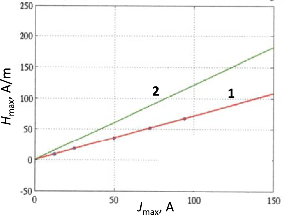
Figure 2 shows dependence of the radiated magnetic field  $H$ calculated numerically at a distance $R=15$ cm as a function of electric current in the stalk $J$ and evaluated from Equation (4). The good agreement confirms the usefulness of a simplified analytical approach for quick evaluation of the radiated field. Linear dependence of the radiated field on the current indicates the way to proceed for the EMP mitigation: one has to reduce the current through the stalk by increasing the discharge time.
The intensity of GHz emission can be affected by changing the stalk material and/or reducing the velocity of the propagation of the current. By using a dielectric stalk, one increases its resistance and consequently reduces the return current[Reference Bradford, Woolsey, Scott, Liao, Liu, Zhang, Zhu, Armstrong, Astbury, Brenner, Brummitt, Consoli, East, Gray, Haddock, Huggard, Jones, Montgomery, Musgrave, Oliveira, Rusby, Spindloe, Summers, Zemaityte, Zhang, Li, McKenna and Neely52]. Another possibility is to increase the effective time of current propagation between the target and the ground by making the stalk in a form of a spiral. For a spire radius  $r$ and a pitch $h$, the speed of current propagation along the spiral axis $v_{\Vert }$ is reduced by a factor $2\unicode[STIX]{x1D70B}r/h$, and consequently the major emission frequency $hc/4l_{s}r$ is not compatible with the antenna length. The emission power is expected to decrease by a factor $(2r/h)^{2}$. The authors of Ref. [Reference Bradford, Woolsey, Scott, Liao, Liu, Zhang, Zhu, Armstrong, Astbury, Brenner, Brummitt, Consoli, East, Gray, Haddock, Huggard, Jones, Montgomery, Musgrave, Oliveira, Rusby, Spindloe, Summers, Zemaityte, Zhang, Li, McKenna and Neely52] reported suppression of the emitted signal by a factor of 30 by using a plastic spiral compared to a straight aluminum stalk (see Section 4.1 for more details).
This simple analysis also explains why the ps laser pulses are much stronger emitters in the GHz domain, compared to the ns pulses. The former accumulate a big charge for a short period of time and discharge it in a short and intense current pulse. In contrast, the latter induce a relatively weak continuous current and consequently a much weaker emission. The authors of Ref. [Reference Cikhardt, Krása, De Marco, Pfeifer, Velyhan, Krouský, Cikhardtova, Klír, Řezáč, Ullschmied, Skala, Kubes and Kravarik54] present the measurements of the EMP emission in the GHz domain produced with laser pulses of intermediate duration of 300 ps, which is shorter than the period of the return current oscillations but longer than the electron cooling time. Consequently, electron ejection persists during the whole driving laser pulse and the emission spectrum extends to lower frequencies in the MHz domain, but its intensity decreases with frequency[Reference Krása, Giuffrida, Side, Klír, Cikhardt and Řezáč45, Reference Krása, De Marco, Cikhardt, Pfeifer, Velyhan, Klír, Řezáč, Limpouch, Krouský, Dostál, Ullschmied and Dudžák55].
The EMP signal can be significantly enhanced if a long and a short laser pulses interact with the same target. In Ref. [Reference Miragliotta, Spicer, Brawley and Varma56], the emission caused by ultrashort (38 fs, 35 mJ, 800 nm) laser pulse ablation at atmospheric pressure of a metal target was observed to be enhanced by an order of magnitude due to a preplasma generated on the same target by a different, long-pulse laser (14 ns, 205 mJ, 1064 nm). The same effect was described in Ref. [Reference Varma, Spicer, Brawley and Miragliotta57] in the case of glass and copper targets.
Among multiple sources of this emission, we mention the secondary polarization charges induced by ejected electrons on the conducting parts of the chamber[Reference Mead, Neely, Gauoin, Heathcote and Patel9, Reference Bateman and Mead42], emission from a toroidal current circulating in the expanding plasma plume[Reference Felber58] and the plasma recombination after the end of the laser pulse[Reference Krása, Láska, Rohlena, Velyhan, Lorusso, Nassisi, Czarnecka, Parys, Ryć and Wolowski59]. As observed in the previous paragraph, further contributions to the GHz range can come from charged particles emitted from the target inducing secondary dipoles on metallic objects, and from X-rays acting on surfaces of objects exposed to the radiating interaction.
Scheme of target charging in the case of short-pulse interaction with a thick solid target. Hot electrons are created in the laser focal spot (red zone). They spread in the target over a distance comparable to the mean free path (gray zone). The electrons escaping in vacuum create a spatial charge and prevent low-energy electrons from escaping. Electrons with energies higher than the surface potential escape from the target and create a net positive charge at the surface. Reprinted with permission from Ref. [Reference Dubois, Lubrano-Lavaderci, Raffestin, Ribolzi, Gazave, La Fontaine, d’Humières, Hulin, Nicolaï, Poyé and Tikhonchuk13]. Copyright 2014 by the American Physical Society.
2.3 Modeling of the electron emission
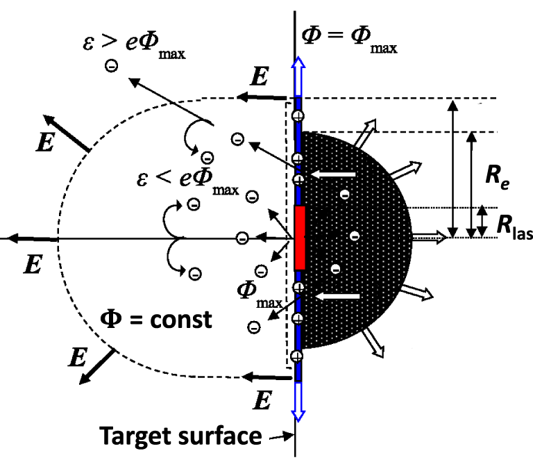
Ejection of energetic electrons is identified as the dominant source of target charging. This process is shown schematically in Figure 3, assuming that the target size is larger than the hot electron mean free path. The target charging process can be described by the following steps.
(1) The laser pulse deposits its energy at the target surface. It is partially transferred to the hot electrons with conversion efficiency $\unicode[STIX]{x1D702}_{\text{las}}$. Their energy distribution can be approximated by a Maxwellian function with the effective temperature $T_{h}$ given by Equation (1).
(2) The electrons accelerated in the backward direction are ejected from the target in vacuum, thus creating an initial potential
$\unicode[STIX]{x1D6F7}$ near the target surface. This potential confines the major part of escaping electrons in the Debye layer and returns them back to the target.(3) The hot electrons are accelerated in the forward direction and propagate outside the laser focal spot. Their diffusion is dominated by the elastic collisions with the target ions, and collisions with the target electrons define their cooling time. It is of the order of a few ps for common metals such as aluminum or copper.
(4) Some of the scattered hot electrons are ejected from the target as long as their energy remains higher than the electrostatic potential
$\unicode[STIX]{x1D6F7}$. This process is accompanied by the increase of the potential, and it stops as the maximum electron energy equals the potential. Thus, the processes of the potential buildup and electron cooling define the maximal time of the target charging.(5) The deficit of electrons in the laser spot is compensated by the return current of cold electrons, so the charged zone expands radially over the target surface approximately with the light velocity. The hot electron cloud expands also but more slowly with the drift (thermal) electron velocity. For targets thinner than the hot electron mean free path, the electron emission takes place also from the rear side[Reference Poyé, Hulin, Ribolzi, Bailly-Grandvaux, Lubrano-Lavaderci, Bardon, Raffestin, Santos and Tikhonchuk36].


The theoretical model developed in Refs. [Reference Dubois, Lubrano-Lavaderci, Raffestin, Ribolzi, Gazave, La Fontaine, d’Humières, Hulin, Nicolaï, Poyé and Tikhonchuk13, Reference Poyé, Hulin, Ribolzi, Bailly-Grandvaux, Lubrano-Lavaderci, Bardon, Raffestin, Santos and Tikhonchuk36, Reference Poyé, Hulin, Bailly-Grandvaux, Dubois, Ribolzi, Raffestin, Bardon, Lubrano-Lavaderci, d’Humières, Santos, Nicolaï and Tikhonchuk60, Reference Poyé, Dubois, Lubrano-Lavaderci, d’Humières, Bardon, Hulin, Bailly-Grandvaux, Ribolzi, Raffestin, Santos, Nicolaï and Tikhonchuk61] describes the target charge buildup with two equations: the hot electron distribution function  $f_{eh}(\unicode[STIX]{x1D700},t)$ and the electric potential $\unicode[STIX]{x1D6F7}(t)$. The distribution function varies in time due to three processes:
 $$\begin{eqnarray}\unicode[STIX]{x2202}_{t}f_{eh}=S_{\text{las}}(\unicode[STIX]{x1D700},t)-\unicode[STIX]{x1D70F}_{ee}^{-1}f_{eh}-g_{e}(\unicode[STIX]{x1D700},t),\end{eqnarray}$$
 production of the hot electrons with rate  $S_{\text{las}}$, cooling of hot electrons in the electron–electron collisions with characteristic time $\unicode[STIX]{x1D70F}_{ee}$ and ejection of electrons from the target surface with rate $g_{e}$ depending on the potential $\unicode[STIX]{x1D6F7}$. The production rate is assumed to be a Maxwellian function of energy, with the hot electron temperature depending on the laser intensity according to Equation (1). This approximation is in agreement with the observations of energetic electrons produced in laser–plasma interaction and empirical scaling[Reference Wilks, Kruer, Tabak and Langdon32, Reference Beg, Bell, Dangor, Danson, Fews, Glinsky, Hammel, Lee, Norreys and Tatarakis62]. The function is normalized to the linear production of electrons by the laser: $\unicode[STIX]{x1D702}_{\text{las}}E_{\text{las}}/T_{h}t_{\text{las}}$. The electron cooling time can be described by analytical expressions[Reference Kanaya and Okayama63] or taken from the tables[64]. The radius of the emission zone $R_{h}$ increases with time according to the hot electron velocity from the minimum value equal to the laser focal spot to the maximum value equal to the electron mean free path.
The electric potential is represented as a sum of the thermal potential created by the electrons in the Debye layer near the target surface and the positive charge left on the target surface by escaped electrons:  $\unicode[STIX]{x1D6F7}=\unicode[STIX]{x1D719}_{th}+\unicode[STIX]{x1D719}_{E}$. The thermal potential is proportional to the hot electron temperature with an additional factor $\unicode[STIX]{x1D709}$ depending on the ratio of the hot electron Debye radius to the radius of the hot electron cloud on the target surface, $e\unicode[STIX]{x1D719}_{th}=T_{h}\unicode[STIX]{x1D709}(\unicode[STIX]{x1D706}_{Dh}/R_{e})$, and also on the ratio of the Debye length to the target thickness. The electrostatic potential $\unicode[STIX]{x1D719}_{E}$ is proportional to the escaped current $J_{e}=e\int g_{e}\,\text{d}\unicode[STIX]{x1D700}$ distributed over the disc on the target surface with the radius increasing with the light velocity:
 $$\begin{eqnarray}\unicode[STIX]{x1D719}_{E}(t)=\frac{1}{2\unicode[STIX]{x1D70B}\unicode[STIX]{x1D716}_{0}}\int _{0}^{t}\text{d}t^{\prime }\frac{J_{e}(t^{\prime })}{R_{e}(t^{\prime })+c(t-t^{\prime })}.\end{eqnarray}$$
This model is realized numerically as a Fortran 90 program ChoCoLaT2.f90[Reference Poyé, Hulin, Ribolzi, Bailly-Grandvaux, Lubrano-Lavaderci, Bardon, Raffestin, Santos and Tikhonchuk36] and is available on request. This program computes the time evolution of the electron cloud parameters, the evolution of the ejection current distribution and the evolution of the two contributions to the potential barrier. These three important parts of the model are closely interrelated.
Dependence of the target charge  $Q_{e}$ on the laser energy and the pulse duration for the laser spot radius of $6~\unicode[STIX]{x03BC}\text{m}$, the absorption fraction $\unicode[STIX]{x1D702}_{\text{las}}=40\%$ and laser wavelength of $0.8~\unicode[STIX]{x03BC}\text{m}$. The dashed white rectangle shows the domain explored in the experiment. Reprinted with permission from Ref. [Reference Poyé, Hulin, Bailly-Grandvaux, Dubois, Ribolzi, Raffestin, Bardon, Lubrano-Lavaderci, d’Humières, Santos, Nicolaï and Tikhonchuk60]. Copyright 2015 by the American Physical Society.

Figure 4 shows the dependence of the accumulated charge on the laser pulse energy and duration calculated with the model. One can distinguish two different regimes of target charging. First, an almost complete hot electron ejection takes place in the case where  $T_{h}\gtrsim e\unicode[STIX]{x1D6F7}$, where the target charge can be approximated as $Q_{e}\simeq eN_{e}$. Here $N_{e}=\int \int S_{\text{las}}\,\text{d}t\,d\unicode[STIX]{x1D700}$ is the total number of hot electrons. Second, there is a quasi-stationary regime where the laser pulse duration is longer than the hot electron cooling time. In this case, the current of ejected electrons is equal to $J_{e}=Q_{e}/t_{\text{las}}$. Between these two limits there is a thermal regime, where all the features of the model play an important role.
This model demonstrates dependence of the charging process on the laser and target parameters. The number and energy of hot electrons depend primarily on the absorbed laser energy, intensity and focusing conditions. The conventional estimate of hot electron average energy, given in Equation (2), may be altered by effects such as stochastic heating[Reference Morace, Iwata, Sentoku, Mima, Arikawa, Yogo, Andreev, Tosaki, Vaisseau, Abe, Kojima, Sakata, Hata, Lee, Matsuo, Kamitsukasa, Norimatsu, Kawanaka, Tokita, Miyanaga, Shiraga, Sakawa, Nakai, Nishimura, Azechi, Fujioka and Kodama65] and direct laser acceleration under suitable conditions[Reference Robinson, Arefiev and Neely66]. With increase of laser pulse energy and target size, more electrons are ejected. Numerical simulations and experiments discussed in Section 4 show that the target charge is increasing with the laser energy according to a power law  $Q_{e}\propto E_{\text{las}}^{\unicode[STIX]{x1D6FC}}$ with index $\unicode[STIX]{x1D6FC}$ varying between 1 and 0.5 depending on intensity. Increase of the laser focal spot and of the pulse duration for a given absorbed pulse energy results in a decrease of laser intensity and, consequently, of the number of ejected electrons. Dependence of the number of ejected electrons could be more complicated in experiments where laser defocusing is accompanied by a variation of absorption due to nonlinear laser–plasma interaction[Reference Rusby, Gray, Butler, Dance, Scott, Bagnoud, Zielbauer, McKenna and Neely67]. However, laser focal spot and pulse duration have very different consequences if one increases them too much while keeping the laser energy unchanged. As the laser intensity is reduced, there are more electrons produced with a smaller energy. Then, the thermal barrier is also reduced and the electrostatic potential $\unicode[STIX]{x1D719}_{E}$ dominates the barrier. As the latter is not directly related to laser intensity and the electron energy decreases with the laser intensity, the ejected charge $Q_{e}$ is reduced as the laser intensity decreases. Therefore, there is an optimal intensity for the most efficient charging process, as shown in Figure 5. This was confirmed in Ref. [Reference Aktan, Ahmed, Aurand, Cerchez, Poyé, Hadjisolomou, Borghesi, Kar, Willi and Prasad68] by comparing the theoretical estimates made with ChoCoLaT2.f90 with experimental data.
Target charge  $Q_{e}$ in nC calculated from the model as a function of the absorbed laser energy and the focal spot diameter for the pulse duration of 1 ps, wavelength $0.8~\unicode[STIX]{x03BC}\text{m}$ and an insulated and laser size target. There is an optimal spot diameter for the target charging.

We discuss now generation of the neutralization current  $J_{n}$ and introduce the characteristic time of electron ejection $t_{ej}$ as a maximum between the electron cooling time and the laser pulse duration. The electron ejection time can be compared to the time of propagation of the neutralization current along the stalk, $t_{n}=l_{s}/c$. If the neutralization time is longer than the ejection process, the target can be considered as isolated from the ground. Otherwise, the neutralization must be accounted for in the model as it impacts the value of the electrostatic potential. This effect is described by modifying Equation (7) as follows:
 $$\begin{eqnarray}\unicode[STIX]{x1D719}_{E}(t)=\frac{1}{2\unicode[STIX]{x1D70B}\unicode[STIX]{x1D716}_{0}}\int _{0}^{t}\text{d}t^{\prime }\frac{J_{e}(t^{\prime })-J_{n}(t^{\prime })}{R_{e}(t^{\prime })+c(t-t^{\prime })}.\end{eqnarray}$$
 If the neutralization time is much shorter than the electron ejection time, one can equalize the ejection and neutralization currents,  $J_{e}\approx J_{n}$, and set $\unicode[STIX]{x1D719}_{E}=0$. This case of a fully grounded target applies to sufficiently long laser pulses. Here the ejection current is weak, and it does not produce oscillations responsible for EMP generation in the GHz domain.
The target size also has an impact on the charging process. Let us consider a cylinder with its axis aligned with the laser. It is characterized by thickness  $e_{\text{tar}}$ and radius $r_{\text{tar}}$. The target radius defines its charge capacitance. Reduction of the target radius and capacitance results in an increase of the electrostatic potential that has a strong impact on the charging process by reducing the final value of $Q_{e}$. Figure 6 shows the dependence of the target charge on radius $r_{\text{tar}}$. The radius where the target can be considered as infinite depends on the laser energy. This effect was also investigated analytically in Ref. [Reference Poyé, Dubois, Lubrano-Lavaderci, d’Humières, Bardon, Hulin, Bailly-Grandvaux, Ribolzi, Raffestin, Santos, Nicolaï and Tikhonchuk61] and experimentally in Ref. [Reference Ahmed, Kar, Cantono, Hadjisolomou, Poyé, Gwynne, Lewis, Macchi, Naughton, Nersisyan, Tikhonchuk, Willi and Borghesi69].
Target charge  $Q_{e}$ in nC calculated from the model as a function of the absorbed laser energy and the target diameter for the pulse duration of 1 ps, the focal spot diameter of $10~\unicode[STIX]{x03BC}\text{m}$, wavelength of $0.8~\unicode[STIX]{x03BC}\text{m}$ and an insulated target. There is a threshold on the target diameter below which the target charging becomes dependent on it.

The target thickness can vary from large values where hot electrons never reach the rear side to very small values  ${\sim}10~\unicode[STIX]{x03BC}\text{m}$, which are comparable with the Debye length of the hot electron cloud $\unicode[STIX]{x1D706}_{Dh}$. The target thickness has two effects on the charging process. First, if the hot electron mean free path is larger than the target thickness, the electrons are trapped inside the target and recirculate; the current increases because of ejection, which takes place from both sides of the target. Second, the thermal potential $\unicode[STIX]{x1D719}_{th}$ has a lower value, if $\unicode[STIX]{x1D706}_{Dh}>e_{\text{tar}}$, which results in a current burst. However, these two effects are mitigated by the electrostatic part of the potential barrier, which increases with the current according to Equation (7). Globally, in thin targets the ejected charge increases by a factor that depends on the laser energy and duration: by 2 times for short pulses of 1 J and by 5 times for short pulses of 0.1 kJ. This has been demonstrated in Ref. [Reference Poyé, Hulin, Ribolzi, Bailly-Grandvaux, Lubrano-Lavaderci, Bardon, Raffestin, Santos and Tikhonchuk36]. The charge accumulation has been compared with experimental data in Refs. [Reference Poyé, Hulin, Ribolzi, Bailly-Grandvaux, Lubrano-Lavaderci, Bardon, Raffestin, Santos and Tikhonchuk36, Reference Aktan, Ahmed, Aurand, Cerchez, Poyé, Hadjisolomou, Borghesi, Kar, Willi and Prasad68].
The target crystalline structure also affects the electron mean free path and consequently the accumulated electron charge. In experiments with targets made of different allotropes of carbon in Ref. [Reference McKenna, Robinson, Neely, Desjarlais, Carroll, Quinn, Yuan, Brenner, Burza, Coury, Gallegos, Gray, Lancaster, Li, Lin, Tresca and Wahlström70], it was found that the highly ordered lattice structure of diamond at temperatures of the order of 1–100 eV results in longer electron mean free path and suppression of electron beam filamentation compared to less ordered forms of carbon.
In the study described in Ref. [Reference Xia, Zhang, Cai, Zhou, Tian, Zhang, Liu, Yi, Xu, Wang, Li and Zhu71], a laser pulse (1 ps, 100 J) irradiated  $200~\unicode[STIX]{x03BC}\text{m}$ thick CH targets doped with different titanium (Ti) concentrations at the XG-III laser facility. The observed EMP emission was related to the hot electrons ejected from the target surface in the forward direction. The EMP intensity increased by a factor of 2 when doping increased from $1\%$ to $7\%$ and then slightly decreased. This behavior is explained by an increase of the target conductivity and laser absorption due to the doping, which favored hot electron emission in the forward direction.
2.4 Numerical modeling of the EMP emission
Because of the large disparity of temporal scales, the process of electron emission needs to be simulated in several subsequent steps by using different numerical tools. First, the hot electron production during the interaction of an intense laser pulse with a solid target depends strongly on the quality of the target surface at the moment of laser pulse arrival. It may be modified by the laser prepulse and affect the absorption of the main laser pulse. The preplasma formation and its expansion from the solid target surface is described with a radiation hydrodynamic code on the ns timescale. Secondly, as the main laser pulse interaction with the plasma and hot electron generation are kinetic processes, they are simulated in detail with a relativistic particle-in-cell (PIC) code. This fully kinetic simulation is however limited to a characteristic time of the order of 1 ps and to a spatial size of a few tens of microns. Moreover, the electron collisions are described in a simplified manner. For these reasons, at the third step, the electron distribution calculated with a PIC code is transferred to a Monte Carlo particle transport code describing the propagation of hot electrons in the solid target, their collisions and secondary reactions. It provides the number and the energy distribution of the escaped electrons.
Numerical simulations reported in Ref. [Reference Dubois, Lubrano-Lavaderci, Raffestin, Ribolzi, Gazave, La Fontaine, d’Humières, Hulin, Nicolaï, Poyé and Tikhonchuk13] were performed with the laser intensity  $2\times 10^{18}~\text{W}\cdot \text{cm}^{-2}$, laser wavelength of $0.8~\unicode[STIX]{x03BC}\text{m}$, pulse duration of 50 fs and focal spot radius of $4~\unicode[STIX]{x03BC}\text{m}$. According to the PIC simulations, about 40% of the incident laser energy was transferred to hot electrons in the copper target with a temperature $T_{h}\simeq 250$ keV. The PIC simulation box was however too small to distinguish between the escaped and trapped electrons. The Monte Carlo simulation shows that about 35% of the hot electrons injected in the target are scattered back into the vacuum. Their energy is 2–3 times larger than the hot electron temperature.
The current decreases by an order of magnitude in 2 ps after the laser pulse and the emission zone is limited effectively by the radius of  $10~\unicode[STIX]{x03BC}\text{m}$. These numbers are consistent with the expected lifetime of hot electrons and their mean free path. The emission continues for a few tens of ps and the emission zone extends to a few mm, but more than 90% of the total charge was emitted in the first 2 ps. At that moment, the target is charged to a potential of about 200 kV compatible with the hot electron temperature.
A Monte Carlo transport code describes single particle motion in matter, but it does not account for collective effects and self-consistent electromagnetic fields. Therefore, it cannot describe the electromagnetic emission. The fourth stage of EMP modeling was performed with a large-scale electromagnetic PIC code SOPHIE[Reference Cessenat53] describing the collective motion of electrons in free space with prescribed boundary conditions on the surfaces. The electron emission from the target was described with current density calculated using a Monte Carlo code as shown in Figure 7(a). The simulation was performed in a box of volume of a few  $\text{mm}^{3}$ and for a time of 40 ps. Figure 7(b) shows the current of ejected electrons recorded at the other surface of the simulation box at a distance of 1 mm from the target surface. This distance is much larger than the hot electron Debye length, and consequently it describes the electron bunch that escaped from the target. As it follows from three simulations with different target sizes, the escaped electron charge does not depend on the target size. It has a rising part of 2–3 ps duration, corresponding to the separation of the electron bunch from the target, and a slowly decreasing part, corresponding to the tail of the electron bunch. The delay of 3.5 ps between the ejected and recorded currents corresponds to the time of electron propagation from the target to the recording surface. The electromagnetic emission is generated in the rising part of the current, and it corresponds to the THz pulse described in Section 2.2.1.
(a) Time dependence of the current density of electrons emitted backward from the target surface at different distances from the laser axis obtained in the Monte Carlo simulation. (b) Time dependence of the electric current of escaped electrons collected at a distance of 1 mm from the target. Three simulations with the target radii 2.5, 5 and 7.5 mm are shown. The dashed line shows the ejection current obtained from the Monte Carlo simulation. Reprinted with permission from Ref. [Reference Dubois, Lubrano-Lavaderci, Raffestin, Ribolzi, Gazave, La Fontaine, d’Humières, Hulin, Nicolaï, Poyé and Tikhonchuk13]. Copyright 2014 by the American Physical Society.

(a) Simulation of the current at the bottom of the target assembly. Calculation with the SOPHIE code: the target radius is 5 mm, the laser pulse energy is 80 mJ and the pulse duration is 50 fs. The current is collected at an effective  $50\,\unicode[STIX]{x03A9}$ resistance. (b) Comparison of the calculated waveform (red solid line) with the experimental data (blue dots). Reprinted with permission from Ref. [Reference Dubois, Lubrano-Lavaderci, Raffestin, Ribolzi, Gazave, La Fontaine, d’Humières, Hulin, Nicolaï, Poyé and Tikhonchuk13]. Copyright 2014 by the American Physical Society.

The GHz emission was described in additional numerical simulation with the code SOPHIE on much larger temporal and spatial scales and by taking into account the boundary conditions in the whole experimental chamber, including the target, stalk and all other elements. Figure 8(a) shows the simulated volume of 1  $\text{m}^{3}$ and position of the target and the stalk. In this case, the spatial resolution of 1 mm is poorer than in the previous case but the simulation was run for a longer time of a few ns, and the return current collected at a resistance placed near the ground plate is shown in Figure 8(b). The duration of this current is more than 100 ps, much longer than the ejection current and the current of ejected electron bunch shown in Figure 7(b). As explained in Section 2.2.2, the duration of the return current is proportional to the target size. Correspondingly, the amplitude of the return current is more than one order of magnitude smaller than the current of the ejected electron bunch.
A similar numerical model of EMP generation caused by electron emission is described in Ref. [Reference Jin, Meng, Jiang, Wu and Xu72]. In this case, the EMP associated with emitted electrons was computed with a specially designed code EMPIC-2D. Dependence of the EMP signal on the target size, laser pulse duration and intensity is consistent with the results presented in this review.
The numerical simulations discussed so far confirm the theoretical estimates discussed in Section 2.2 and the major results of the simplified model presented in Section 2.3. While the detailed numerical simulations provide a rather accurate quantitative description of the emission process, they are time-consuming and cannot be performed for all possible experimental conditions. The simplified model is less precise; it may differ by a factor 2–3 and thus provides a more qualitative estimate, but it is much faster and might be sufficient for a quick evaluation of the EMP amplitude.
2.5 Intense transient fields due to deposition of charged particles
Charge emitted by intense laser–target interactions can be efficiently deposited onto objects present within the chamber and, in particular conditions, may give rise to the generation of very large transient electric fields, even rather far from the interaction point. A scheme of this phenomenon is shown in Figure 9.
Scheme of the field induced due to charge deposition on one plate of a capacitor–collector setup. The system is initiated by a flow of energetic particles from a pulsed laser-driven source. Reprinted from Ref. [Reference Consoli, De Angelis, Robinson, Giltrap, Hicks, Ditter, Ettlinger, Najmudin, Notley and Smith73] under Creative Commons license.

This was demonstrated for energetic petawatt-range laser–matter interactions[Reference Consoli, De Angelis, Robinson, Giltrap, Hicks, Ditter, Ettlinger, Najmudin, Notley and Smith73] using the Vulcan Petawatt laser at the Rutherford Appleton Laboratory (RAL), operating at a wavelength of 1054 nm[Reference Edwards, Danson, Hutchinson, Neely and Wyborn74]. Pulses of  ${\sim}1$ ps duration were focused by an off-axis parabolic mirror at an intensity above $10^{20}~\text{W}\cdot \text{cm}^{-2}$ on parylene-N foil targets at normal incidence. The experimental setup is shown in Figure 10. Thomson spectrometers were used to detect particles emitted by the target normal sheath acceleration (TNSA) process[Reference Macchi, Borghesi and Passoni75] in forward (TS2 and TS3) and backward (TS1) directions with respect to the incoming laser. The focusing parabola consisted of a 110 mm thick, 650 mm diameter glass substrate with a 620 mm diameter silver front surface, placed at 1.8 m from the target.
Top-view scheme of the vacuum chamber; the laser (red beam) is focused on a thin-foil target by an off-axis parabola mirror. Reprinted from Ref. [Reference Consoli, De Angelis, Robinson, Giltrap, Hicks, Ditter, Ettlinger, Najmudin, Notley and Smith73] under Creative Commons license.

The AD-80D(R) D-dot differential electric field sensor[76] (3 dB bandwidth up to 5.5 GHz) (see Section 3.2.1) was placed behind the parabola mirror, which provided good isolation from direct particle and ionizing electromagnetic radiation fluxes from the target. It was at  ${\sim}2.2$ m overall distance from origin, with its sensitive direction (normal to its ground plane): $\hat{u} =0.12\hat{x}+0.87{\hat{y}}+0.49\hat{z}$. The position and orientation were set for efficient protection against initial direct ionizing radiation due to the laser–matter interaction. The BIB-100G balun (250 kHz–10 GHz bandwidth) was connected to its terminals for a high rejection of common-mode disturbances. Details of the measurement methods for this specific experiment are supplied in Section 3.2.4.
(a)  $V_{\text{DDOT}}$ signal detected by the D-dot probe in shot $\#29$; (b) time-gated normalized spectrogram of the signal. The origin of the timescale was set at the moment when the EMP signal reaches the D-dot probe. Reprinted from Ref. [Reference Consoli, De Angelis, Robinson, Giltrap, Hicks, Ditter, Ettlinger, Najmudin, Notley and Smith73] under Creative Commons license.

(a) Component of the electric field normal to the D-dot ground plane measured in shot #29. (b) Comparison of several single-shot measurements of the electrical field component normal to the D-dot ground plane.

For shot #29 (269 nm target thickness, 386 J laser energy and  $4.8\times 10^{20}~\text{W}\cdot \text{cm}^{-2}$ intensity), the resulting $V_{\text{DDOT}}$ signal stored by the oscilloscope is shown in Figure 11(a). At first sight, the trace looks like a classical EMP generated by laser–plasma interaction, with a fast rise followed by an envelope with an exponential decay. The time-resolved spectrogram of this signal (see Section 2.6.2) is given in Figure 11(b), and shows that indeed a low-frequency component (LFC) is present only in the 40–80 ns interval, while the high-frequency component (HFC) is present from the beginning over a larger time interval and has a broad spectrum up to 6 GHz.
Through a process of accurate cable frequency-domain de-embedding (see Section 3.1) and numerical time integration, the component of the applied electric field normal to the D-dot ground plane was determined, as shown in Figure 12(a). Both the LFC and HFC can be clearly seen. In particular, the broadband HFC appears as a modulation with respect to the LFC; it has a maximum peak-to-peak amplitude  $\unicode[STIX]{x0394}E_{\text{HFC-pp}}\sim 172$ kV/m, visible in the (0, 30) ns time interval and gradually decreases with time. This is the classical form of EMP due to a laser–plasma interaction. Concerning the LFC, the field increases over the interval (30, 93) ns time to $\unicode[STIX]{x0394}E_{\text{LFC}}\sim 600$ kV/m. The field rise is delayed with respect to the laser pulse, and can be readily associated with charges reaching the focusing parabola and depositing on its surface. Neutralization of the deposited charge on the parabola can occur later in time due to either particles of opposite charge arriving at later times or charge relaxation processes with a time constant governed by the parabola structure and its support.
Figure 12(b) shows the comparison of electric field profiles obtained by D-dot measurements when shooting with similar laser energy on targets made of the same plastic but of different thicknesses. Higher fields are generated for targets with smaller thickness. Indeed, this is also the condition to achieve more accelerated particles, also at higher energy, in a classical TNSA scheme[Reference Macchi, Borghesi and Passoni75]. The rise of the electric field depends on the shot and for the thinnest target (shot  $\#16$) occurs earlier with respect to the others, as expected for more energetic protons. These considerations are confirmed by the spectrum of protons detected by the TS1 spectrometer in the backward direction for the shots #16 and #29[Reference Consoli, De Angelis, Robinson, Giltrap, Hicks, Ditter, Ettlinger, Najmudin, Notley and Smith73].
Proof-of-principle numerical simulations were performed by CST Particle Studio three-dimensional (3D) PIC code to get a suitable description of the field development due to charged particle dynamics in the considered setup. The parabola was modeled as a thin silver layer on a thick glass cylinder, mounted on a stainless steel annular holder. Secondary-electron emission and superficial charge deposition were computed on all surfaces. Space-charge effects were also calculated, but the overall bunch charge was kept to low values to minimize them. For each particle species, emission was uniformly distributed within a  $\unicode[STIX]{x1D703}=20^{\circ }$ angle to target normal, and also uniform in velocity within a given particle kinetic range.
The optimization process was performed to get a suitable qualitative fit to the experimental data of D-dot probe shown in Figure 12(a). An energy range  $(0.774,2.68)$ MeV and 35 nC overall charge was determined for protons, and $(9.40,34.7)$ keV and 7.5 nC for electrons. Figure 13 shows a comparison of the normalized D-dot measurements and simulation results for shot #29 at the same position, for both $x$ and $u$ (the sensitive D-dot axis normal to its ground plane) components of the electric field. Even with this rather simple model, a close agreement is reached, and the optimized proton energy range is in good correspondence with the most energetic part of spectrum measured by TS1[Reference Consoli, De Angelis, Robinson, Giltrap, Hicks, Ditter, Ettlinger, Najmudin, Notley and Smith73].
Comparison between experimental D-dot measurements from shot #29 and PIC simulations of electric fields at the D-dot position, in the  $\hat{u}$ and $\hat{x}$ directions. The origin of the timescale is here set at the moment of laser–target interaction, and the #29 measurement was thus time-shifted, with respect to Figures 11 and 12, by the EMP propagation time from target to D-dot probe. Reprinted from Ref. [Reference Consoli, De Angelis, Robinson, Giltrap, Hicks, Ditter, Ettlinger, Najmudin, Notley and Smith73] under Creative Commons license.

In experiments of this type, intense UV, X and  $\unicode[STIX]{x03B3}$ bursts were produced at the moment of laser–target interaction, together with beams of relativistic electrons. The electromagnetic contribution is capable of generating photoionization on any exposed surface, and can thus create a layer of emitted electrons with energies of a few eV surrounding it and leave a transient superficial positive charge. On a slightly longer timescale, MeV-range relativistic electrons are expected to deposit a negative charge on the same surfaces, since secondary-electron emission at those energies is smaller than unity[Reference Consoli, De Angelis, Robinson, Giltrap, Hicks, Ditter, Ettlinger, Najmudin, Notley and Smith73]. These two processes operate in opposite directions, and it is not trivial to estimate the electric fields due to their superimposition. Indeed, no associated field was observed during the early moments shown in Figure 12(a), perhaps because it was hidden by the contemporary presence of the HFC due to classical EMP. This was the reason why in the PIC simulations only one low-energy component was considered for the electrons, which was sufficient to give a good phenomenological description of the process observed experimentally.
2.6 Methods of description for EMP signals
2.6.1 Modal structure of the fields in the vacuum chamber
The duration of EMP fields extends over a time much longer than the laser pulse. The average dimensions of a vacuum chamber used in experiments of laser–matter interaction is up to a few meters, and thus the microwave electromagnetic waves undergo multiple reflections on the objects usually present within the chamber, and especially on its walls, floor and roof. Consequently, the quasi-modal structure of fields in such a resonant cavity is settled out after tens of reflections, corresponding to an overall transient time of a few hundreds of ns. The electromagnetic field inside the vacuum chamber can be mathematically represented as the weighted sum of an orthogonal set of proper modes[Reference Consoli, De Angelis, Andreoli, Cristofari and Di Giorgio77–Reference Van Bladel79]:
 $$\begin{eqnarray}\displaystyle \begin{array}{@{}c@{}}\mathbf{E}=\displaystyle \mathop{\sum }_{i=1}^{+\infty }A_{i}\mathbf{E}_{i}+\displaystyle \mathop{\sum }_{i=1}^{M-1}A_{i}^{0}\mathbf{E}_{i}^{\,0}+\displaystyle \mathop{\sum }_{i=1}^{+\infty }B_{i}\mathbf{s}_{i},\\ \mathbf{H}=\displaystyle \mathop{\sum }_{i=1}^{+\infty }C_{i}\mathbf{H}_{i}+\displaystyle \mathop{\sum }_{i=1}^{P-1}C_{i}^{\,0}\mathbf{H}_{i}^{\,0}+\displaystyle \mathop{\sum }_{i=1}^{+\infty }D_{i}\mathbf{g}_{i},\end{array} & & \displaystyle\end{eqnarray}$$
 where  $\mathbf{E}_{i}$ and $\mathbf{H}_{i}$ are the solenoidal electric and magnetic eigenvectors; $\mathbf{E}_{i}^{\,0}$ and $\mathbf{H}_{i}^{\,0}$ are the harmonic electric and magnetic eigenvectors, associated with $M$ separate boundary parts and with a P-times connected volume, respectively; and $\mathbf{s}_{i}$ and $\mathbf{g}_{i}$ are the irrotational electric and magnetic eigenvectors.
The determination of the coefficients of this expansion is obtained by resolving a system of linear equations. In the most general case, these coefficients are functions of time. They contain the coupling integrals[Reference Conciauro, Guglielmi and Sorrentino78, Reference Van Bladel79] of the single modes with the impressed sources: electrical currents in the medium contained in the resonator and external electromagnetic waves coupled to the resonator through proper apertures on its boundaries. Equation (9) contains an infinite number of modes, but only few of them are actually excited by the sources, resulting in a finite number of coupling integrals[Reference Van Bladel79]. In particular, solenoidal terms with large coefficients  $A_{i}$ and $C_{i}$ are dominant for frequencies $\unicode[STIX]{x1D714}\sim \unicode[STIX]{x1D714}_{i}=k_{i}c$, where $k_{i}$ is the eigenvalue associated with the $i$th solenoidal eigenvector.
For a primary EMP pulse of short time duration and broadband spectrum, the cavity acts as a microwave filter. A given excited resonant solenoidal mode persists for a long time depending on its quality factor  $Q_{i}$, while other harmonic components of the original EMP pulse, not effectively coupled to other modes, decay rather fast. The quality factor is related to the time of energy variation in the chamber as $Q_{i}=2\unicode[STIX]{x1D70B}\bar{W}_{i}/{\dot{W}}_{i}$, where $\bar{W}_{i}$ is the time-average energy stored in the chamber at the resonant mode and ${\dot{W}}_{i}$ is the energy lost per cycle due to dissipation or to any other leakage from the resonator[Reference Van Bladel79]. For an ideal Dirac $\unicode[STIX]{x1D6FF}$-function excitation, the mode decays exponentially with a characteristic decay time $\unicode[STIX]{x1D70F}_{i}=2Q_{i}/\unicode[STIX]{x1D714}_{i}$ depending on the quality factor[Reference Slater80].
It is also possible that persistent EMP signals might be due, for particular time intervals, to sources of field placed within the chamber and with specific time and spatial profile, having a frequency content that does not necessarily match one or more of the resonant modes. This can occur for transient field sources, and in this case their fields would be represented by the expansion of harmonic and irrotational vectors in Equation (9).
For a hollow chamber having a simple shape, it is possible to determine the eigenfunctions and eigenvalues analytically. However, conductive objects present in a real experimental chamber may significantly change the modal distribution. These situations can be analyzed with 3D electromagnetic simulations[Reference Consoli, De Angelis, Andreoli, Cristofari and Di Giorgio77, Reference Van Bladel79].
The modal structure of the electromagnetic fields is also modified by hot electrons and plasma expanding from the target. They move rapidly from the interaction point, fill the experimental chamber and influence the space and time characteristics of transmitted and reflected electromagnetic waves. In particular, expanding plasma may reflect EMP waves with wavelengths longer than the critical wavelength associated with the electron density. Thus, within the experimental chamber, a time-varying volumetric distribution of critical regions may be created for each EMP wavelength[Reference Zhang, Xia, Yi, Wang, Wang and Li81, Reference Krása, Consoli, Cikhardt, Pfeifer, De Angelis, Krupka, Klír, Řezáč, Dostál, Krůs and Dudžák82]. Depending on the specific interaction regime, the actual spatial distribution of the electromagnetic fields within the experimental chamber can be strongly modified, and its detailed analysis requires extended numerical simulations.
2.6.2 Time-domain and spectral-domain analysis of EMP signals
The EMP signals and discharge currents measured on different laser facilities have a complex temporal structure. A suitable way to describe the time-domain measurements is the amplitude envelope approach[Reference Consoli, De Angelis, Andreoli, Cristofari and Di Giorgio77, Reference Consoli, De Angelis, Andreoli, Cristofari, Di Giorgio and Ingenito83] characterizing the amplitude variations of the signal. The amplitude envelope AE of a real signal  $x(t)$ is defined as[Reference Boashash84]
 $$\begin{eqnarray}\text{AE}(t)\equiv \left|x(t)+\frac{i}{\unicode[STIX]{x1D70B}}\text{PV}\int _{-\infty }^{+\infty }\frac{x(\unicode[STIX]{x1D70F})}{t-\unicode[STIX]{x1D70F}}\,\text{d}\unicode[STIX]{x1D70F}\right|,\end{eqnarray}$$
 where the second term on the right-hand side represents the Hilbert transform of  $x(t)$ and PV stands for the Cauchy principal value of the integral. For a classical signal containing a sinusoidal carrier modulated in amplitude, AE is equal to the modulating signal. As shown in Figure 14, AE provides a good description of time variations of the signal envelope for the detected signals[Reference Consoli, De Angelis, Andreoli, Cristofari, Di Giorgio and Ingenito83].
Examples of time-domain signals measured with Antennas (a) 1 and (b) 2 for shot  $\#1525$ inside the vacuum chamber of the ABC facility and (c), (d) the corresponding amplitude envelopes obtained from Equation (10). See Table 3 in Section 2.7.2 for further details. Reprinted with permission from Ref. [Reference Consoli, De Angelis, Andreoli, Cristofari, Di Giorgio and Ingenito83]. Copyright 2015 by the IEEE.

The EMP signals generated in the laser–target interactions have a rather fast rise and a slow decay, similar to EMPs generated in nuclear explosions[Reference Lee5]. Thus, the shape of EMP signals can be modeled in time domain as the difference of two exponential functions with two different time constants[Reference Krása, De Marco, Cikhardt, Pfeifer, Velyhan, Klír, Řezáč, Limpouch, Krouský, Dostál, Ullschmied and Dudžák55, Reference Mao and Zhou85, Reference Edgel86], multiplied by a Heaviside step function  $u(t)$[Reference Lee5]:
 $$\begin{eqnarray}f(t)=A_{0}\left[\exp \left(-\frac{t}{\unicode[STIX]{x1D70F}_{f}}\right)-\exp \left(-\frac{t}{\unicode[STIX]{x1D70F}_{r}}\right)\right]\,u(t).\end{eqnarray}$$
Fast Fourier transform (FFT) is commonly used to analyze the spectral content of the signals. However, as can be seen from the example shown in Figure 14, the spectral content of the EMP signals changes over time. Temporal evolution of the EMP spectrum can be obtained through a time–frequency analysis by using the short-time Fourier transform (STFT)[Reference Consoli, De Angelis, Andreoli, Cristofari, Di Giorgio and Ingenito83, Reference Eder, Throop, Brown, Kimbrough, Stowell, White, Song, Back, MacPhee, Chen, DeHope, Ping, Maddox, Lister, Pratt, Ma, Tsui, Perkins, O’Brien and Patel87] defined as[Reference Boashash84]
 $$\begin{eqnarray}F_{x}^{w}(t,f)\equiv \int _{-\infty }^{+\infty }x(\unicode[STIX]{x1D70F})w(\unicode[STIX]{x1D70F}-t)e^{-2\unicode[STIX]{x1D70B}if\unicode[STIX]{x1D70F}}\,\text{d}\unicode[STIX]{x1D70F},\end{eqnarray}$$
 where  $x(t)$ is the time-domain signal and $w$ is a window function being zero outside a specific time interval. A Hamming window function is a recommended option. The associated spectrogram is defined as
 $$\begin{eqnarray}S_{x}^{w}(t,f)\equiv \left|F_{s}^{w}(t,f)\right|^{2}.\end{eqnarray}$$
 According to the Nyquist–Shannon theorem, the sampling rate of the signal  $x(t)$ sets a limit to the maximum frequency in the FFT. Moreover, the frequency resolution depends on the number of acquired samples. This applies also to the STFT[Reference Boashash84]. In practice, Fourier transform is performed in consecutive time intervals, which overlap with each other over a fixed time interval. In this way, time and frequency contents are correlated, but higher time resolution implies a lower frequency resolution and vice versa. An example of STFT description is given in Figure 21 for signals shown in Figure 14.
2.7 Experiments and modeling of EMP signals on several laser facilities
2.7.1 EMP experiments on Vulcan Petawatt laser facility (RAL)
The Vulcan laser facility was one of the first petawatt lasers commissioned in Europe, operational since the early 2000s at the RAL in the UK. It delivers pulses with duration  ${\sim}0.5{-}1$ ps and energy of a few hundred joules at a wavelength of 1054 nm[Reference Edwards, Danson, Hutchinson, Neely and Wyborn74].
Antenna waveforms from a Vulcan shot #13. Reprinted with permission from Ref. [Reference Mead, Neely, Gauoin, Heathcote and Patel9]. Copyright 2004 by the American Institute of Physics.

First measurements of the EMP generated by the Vulcan Petawatt laser were made inside the vacuum chamber in December 2003[Reference Mead, Neely, Gauoin, Heathcote and Patel9] by Möbius loop antennas[Reference Duncan88] (see Section 3.2.2). They were orientated to measure the vertical and transverse (east–west (E/W)) fields. Typical waveforms taken with 300 MHz oscilloscopes are given in Figure 15. These show harmonics and high-frequency noise, which are reduced when the signals are integrated to give the magnetic field. These results are typical of those obtained for ps irradiation of aluminum and copper foil targets with beam energy varying from 330 to 450 J.
The waveforms shown in Figure 15 display the behavior of a system with two weakly coupled modes of slightly different frequencies. The EMP pulse excites a vertical H-mode and then energy is transferred slowly to a transverse H-mode. The latter has a smaller amplitude, which varies at the beat frequency. The waveforms were integrated to give a voltage proportional to the magnetic field and then Fourier-transformed to find the frequencies of the modes shown in Figure 16. The frequency of the vertical H-mode was found to be 63 MHz and the transverse H-mode to be 59 MHz. The peak magnetic field measured at the antenna location was 4.3 A/m in a vertical direction and 0.46 A/m in a transverse direction.
Integrated waveform and FFT of signals shown in Figure 15. Reprinted with permission from Ref. [Reference Mead, Neely, Gauoin, Heathcote and Patel9]. Copyright 2004 by the American Institute of Physics.

The magnitude and frequency of the EMP signal were calculated for an ideal rectangular target chamber. The response of a real target chamber is different due to the effect of equipment inside the chamber, which causes a shift of the resonant frequency and excitation of harmonics.
The Vulcan Petawatt target chamber is a rectangular box of height  $a=2.2$ m, width $b=2$ m and length $d=4.6$ m. The resonant modes of that chamber were calculated analytically[Reference Mead, Neely, Gauoin, Heathcote and Patel9, Reference Ramo, Whinnery and Van Duzer89]. The calculated values of resonant frequency, equivalent capacity, initial voltage and field amplitudes are given in Table 1 for three fundamental modes. The same procedure can be applied also for higher order modes.
Values of different parameters calculated for the fundamental modes of Vulcan Petawatt chamber.

Another experiment that included mode characterization of the same Vulcan Petawatt chamber was performed in 2015[Reference Robinson, Consoli, Giltrap, Eardley, Hicks, Ditter, Ettlinger, Stuart, Notley, De Angelis, Najmudin and Smith90]. A 269 nm thick parylene-N plastic foil target was irradiated with a laser pulse of duration 1.7 ps and energy of 386 J yielding a peak intensity of  $4.8\times 10^{20}~\text{W}\cdot \text{cm}^{-2}$. In this case, a set of electro-optical sensors (see Section 3.3.2) was used for monitoring both the north–south (N/S) and the E/W field components. A D-dot conductive probe (see Section 3.2.1) in another position detected the diagonal field component, that is, a combination of both vertical and horizontal components. The FFT of signals obtained from the optical probes is shown in Figures 17(a) and 17(b), and for the D-dot probe in Figure 17(c).
Frequency spectra of the EMP measured from (a) the north–south and (b) east–west electro-optical probes. (c) Spectrum for signal detected by D-dot probe. Harmonics corresponding to those theoretically expected in chamber and listed in Table 1 are outlined by dashed red vertical lines. Reprinted from Ref. [Reference Robinson, Consoli, Giltrap, Eardley, Hicks, Ditter, Ettlinger, Stuart, Notley, De Angelis, Najmudin and Smith90] under Creative Commons license.

Table 2 summarizes the results for the frequencies of the expected harmonics and spectral peaks detected for all the diagnostics. Several harmonics were detected by the diagnostics but not all of them at the expected frequencies. This is explained by the presence of metallic objects in the chamber such as the silver-plated main focusing parabola, optics mounts, breadboards and other diagnostics. They give rise to multiple additional resonances with similar amplitudes to the hollow cavity modes, and can also shift the resonance frequency of some fundamental cavity modes, or locally change the intensity and direction of fields associated with a given resonant mode, without changing the related resonance frequency[Reference Consoli, De Angelis, Andreoli, Cristofari and Di Giorgio77] (see Section 2.7.2).
Frequencies of the expected harmonics and detected spectral peaks in the Vulcan experiment. Superscript E-W or N-S indicates the mode axis and numbers 1, 2 and 3 indicate the harmonic order.

The D-dot probe results show good correspondence with the expected theoretical values and electro-optic measurements for the 148.5 MHz contribution. An agreement can be also observed for the 202 MHz and 228 MHz harmonics. It is generally difficult to make reliable comparisons between different EMP diagnostics unless they are in identical locations. The presence of metallic objects in the target chamber results in a complex EMP field topology; field strengths and relative amplitudes of spectral components can vary greatly at different positions within the chamber.
Temporal variation in mode frequencies in the Vulcan chamber. Measurements were performed with pulses from the Vulcan laser focused onto a flat target with an  $f/3$ off-axis parabolic mirror at an incident angle of $5^{\circ }$ with respect to the target normal. The pulse duration was 18 ps and laser energies on target varied from 38 to 365 J. The laser was focused to a full-width at half-maximum (FWHM) spot of $5~\unicode[STIX]{x03BC}\text{m}$ at the center of one of the narrow sides of a borosilicate glass with dimensions $0.5~\text{mm}\times 3~\text{mm}\times 3~\text{mm}$. The EMP signal was measured with a Möbius loop, similar to the one used in Ref. [Reference Mead, Neely, Gauoin, Heathcote and Patel9], connected to a 12.5 GHz oscilloscope via a BNC cable. The Möbius loop was located inside the interaction chamber, 1.3 m horizontally from the target and 0.75 m below the horizontal plane. The target was located 1.15 m above the floor and the nearest walls were at distances of 2.3 and 0.9 m. This placed the loop 0.2 m from the chamber wall and approximately 0.4 m from the floor. The maximum frequency that could be resolved by the system was limited by the cabling to $3-4$ GHz. The response of the Möbius loop falls off above 350 MHz and signals above this frequency were thus underestimated. The laser interaction with respect to the start of the Möbius loop measurement occurred at $-20\pm 10$ ns.
Time–frequency analysis with a scanning time window was applied to the EMP measurements to reveal the temporal information associated with the different frequency components in the signal, which would be lost with a standard frequency analysis (see Section 2.6.2). To ensure appropriate frequency and temporal resolution, the scanning time window interval was reduced at higher frequencies with values of 100, 50 and 25 ns being used for the data. Figure 18 shows an example of the time–frequency analysis applied to the field measurements made in two laser shots. The prompt signal seen soon after the laser interaction is observed in both shots and is typically maximized between 0.5 and 1 GHz. The frequencies in this range decay away after 50–150 ns. In Figure 18(b), for the case of the 365 J shot, the prompt signal is higher, as expected, and the strongest of these frequencies have decayed significantly in 50 ns. In addition, lower frequencies in the range of 0.05–0.1 GHz can be seen above the background noise. These lower frequencies rather than appearing immediately after the shot begin to grow 20–50 ns after the shot and last much longer, decaying away after 300 ns. This lower frequency range corresponds to the resonant modes of the Vulcan interaction chamber identified in Ref. [Reference Mead, Neely, Gauoin, Heathcote and Patel9] at 76, 82 and 101 MHz.
Time–frequency analysis of two laser shots. Multiple scanning window sizes have been applied of 100, 50 and 25 ns with transition to the smaller window sizes occurring at 80 and 320 MHz. The laser energy on target was 38 J for (a) and 365 J for (b). For both panels, the color scale represents the amplitude normalized to the scanning window length. The insets in each figure show frequency and time ranges of interest from the main figures. The axes in the insets have the same units as the main figures with the two insets for (b) sharing the same time axis.

The frequencies in the range corresponding to the resonant modes of the chamber are expected to be present for the lower energy shot, but were too weak for the Möbius loop to detect. With the higher laser energy, more electrons were ejected from the target[Reference Gray, Yuan, Carroll, Brenner, Coury, Quinn, Tresca, Zielbauer, Aurand, Bagnoud, Fils, Kühl, Lin, Li, Li, Roth, Neely and McKenna91]; this led to a stronger EMP signal and lower frequencies were detected by the Möbius loop. There is a clear transition from the prompt higher frequencies decaying away as the lower resonant mode frequencies grow at around the time of 50 ns. This qualitatively agrees with the simulation results presented in Figure 30(a), where a transition from the prompt signal stage to a steady stage occurs with the chamber modes being established.
2.7.2 EMP experiments on ABC laser facility (ENEA)
A set of experiments was carried out for studies of modal field distribution on the ABC laser facility operating at the ENEA laboratory in Frascati, Italy, at a fundamental wavelength of 1054 nm with 3 ns pulses[Reference Consoli, De Angelis, Andreoli, Cristofari and Di Giorgio77, Reference Consoli, De Angelis, Andreoli, Cristofari, Di Giorgio and Ingenito83]. Two counterpropagating and synchronized laser beams interacted on opposite sides of a planar target at normal incidence. The experimental data were compared with theoretical and numerical studies of modal field distribution in the interaction chamber and field leakage outside.
A first-order representation of the electromagnetic field distribution within the chamber was obtained by analytically modeling it as a hollow spherical cavity of diameter  $a=1.5$ m. The eigenvalues and the associated resonance frequencies were determined for both TM and TE modes. The frequencies of the first five normal modes are[Reference Conciauro, Guglielmi and Sorrentino78] 174.5 MHz ( $\text{TM}_{m11}$), 246.2 MHz ( $\text{TM}_{m21}$), 285.9 MHz ( $\text{TM}_{m11}$), 316.4 MHz ( $\text{TM}_{m31}$) and 366.7 MHz (TE $_{m21}$). To analyze the mode structure in the real chamber, a set of 3D electromagnetic simulations was performed with the COMSOL numerical solver. Several objects were randomly placed within the cavity. This is illustrated for the case where four conducting cylinders of 75 mm diameter were inserted in the spherical chamber and electrically connected to it (see Figure 19(a)). Their upper base was 37.5 mm below the equatorial plane of the sphere; they were placed parallel and symmetrically to the vertical axis at a distance of 375 mm. With respect to the hollow spherical cavity, the results of simulations showed the following.
(1) Creation of some localized modes at higher frequencies due to the reduced mutual distance (Figure 19(b)).
(2) Modal fields with lower resonance frequencies are excited in the whole cavity due to multiple reflections of the primary EMP. This is shown in Figure 19(c) for the first chamber mode having a frequency of 108.6 MHz, much lower than the frequency of mode
$\text{TM}_{m11}$ at 174.5 MHz of the hollow cavity.(3) Field configurations and resonance frequencies are rather similar to the hollow cavity[Reference Conciauro, Guglielmi and Sorrentino78]. This can be seen in Figure 19(d), for a mode analogous to
$\text{TM}_{m11}$ of the hollow cavity.


COMSOL 3D electromagnetic simulations of a cavity with four conducting cylinders inserted and connected to it. (a) Cavity scheme. Electric field distribution for the mode with resonance frequency of (b) 480.3 MHz; (c) 108.6 MHz; and (d) 175.7 MHz. The red arrows indicate the electric field directions; their size and length are associated with the relative field intensity. Reprinted with permission from Ref. [Reference Consoli, De Angelis, Andreoli, Cristofari and Di Giorgio77]. Copyright 2015 by Elsevier B.V.

Two types of probe were used in the experimental campaign: a wideband monopole (WM) antenna[92] (Antenna 1) and a micro-strip super-wideband (SWB) asymmetrical dipole[Reference Barbarino and Consoli93] (Antenna 2), both placed in the chamber, and another WM antenna, identical to the first one, placed outside the chamber (Antenna 3). Both types of antenna have wideband and quasi-omni-directional pattern. Shot parameters and probe results are summarized in Table 3.
Laser energy and intensity, target thickness, and the measured energy and peak–peak amplitude of detected signals for two shots on the ABC facility.

Figure 20 shows the measured signals with three antennas for shot  $\#650$. The vertical dotted lines in these spectra represent the resonance frequencies for the modes of the hollow cavity, useful for a zeroth-order reference.
Modulus of the single-sided Fourier spectrum of signals detected by the three antennas WM inside, SWB inside and WM outside for the shot  $\#650$ at ABC laser. The vertical dotted lines are the first 15 resonance frequencies for the modes of the hollow cavity. Reprinted with permission from Ref. [Reference Consoli, De Angelis, Andreoli, Cristofari and Di Giorgio77]. Copyright 2015 by Elsevier.

The frequency spectra in Figure 19 are plotted up to 1.5 GHz. No higher frequency components were observed, even though the antenna response was attenuated at frequencies lower than 0.8 GHz and was instead enhanced up to a few GHz. Suppression of the signal above 1.5 GHz might be caused by its attenuation due to the long cables connecting antennas with the oscilloscope. Such tens of meters long cables were used to decrease the direct EMP coupling to the scope. The spectral analysis gives strong components at 130 and 410 MHz for Antennas 1 and 2, whereas the 470 MHz component for Antenna 1 has no observable counterpart for Antenna 2. The 130 MHz component has frequency lower than the  $\text{TM}_{m11}$ mode of the hollow cavity, and is detected by both Antennas 1 and 2. Its presence could be reasonably explained by the case (2) of the list above. The case (1) could be applied to all the previous components around 400 MHz. In a few cases, correspondences of some measured peaks with resonances of the hollow spherical cavity are noted, and could be related to the case (3).
The general loose correspondence between spectra of signals inside and outside the chamber (apart from some localized and low amplitude frequency components) and the presence of intense components at low frequency, with maximum up to  ${\sim}400$ MHz, indicate weak coupling of the internal fields to the outside through the quartz windows, since the diameter of these windows is small for these wavelengths. Another explanation of the weak relation of spectra for fields inside and outside the chamber could be additional EMP sources. There were many cables attached to vacuum radiofrequency feedthroughs with external conductors mounted on a plastic section of flange electrically isolated from the chamber. Currents induced on the external conductor of these cables were free to flow outside the chamber, and can be a source of electromagnetic fields with frequencies different from those inside the chamber.
Figure 21 shows the FFT of the signals in shot #1525 on the aluminum target[Reference Consoli, De Angelis, Andreoli, Cristofari, Di Giorgio and Ingenito83]. For all the antennas, there is correspondence of the main components at 140, 200 and 400 MHz. Contributions at low frequencies (up to 50 MHz) are visible for Antenna 1 only. Some spectral contributions are similar to those found for the case of the plastic target, but some differences are visible, especially for the 200 MHz components.
Shot #1525: FFT and normalized spectrograms for the signals acquired by Antennas 1 and 2 inside the chamber. Reprinted with permission from Ref. [Reference Consoli, De Angelis, Andreoli, Cristofari, Di Giorgio and Ingenito83]. Copyright 2015 by the IEEE.

The FFT gives information on the spectral content of a signal on the whole analyzed time interval. We applied also a time–frequency analysis STFT, as described in Section 2.6.2. Figure 21 shows the application of STFT to signals of antennas inside the interaction chamber. The spectral components from Antennas 1 and 2 at 200 and 400 MHz are similar, but the one at 200 MHz from Antenna 2 lasts for a longer time and it is time-delayed with respect to the others. Two parallel white dashed lines are drawn to outline the time delay. The 140 MHz contribution is observed for both antennas (although less definite for Antenna 1), and it is synchronized with the onset of the 400 MHz component. The electromagnetic fields inside the experimental chamber have time duration up to 100 ns, and spectral content changing with time. This multi-component nature of the signals might be due to the superimposition of modal fields localized within the experimental chamber and modified by the presence of conductive objects inside, giving rise to higher resonance frequencies.
2.7.3 EMP experiments on Asterix IV laser facility (PALS)
Asterix IV is an iodine laser system delivering a pulse of 300 ps duration with energy up to 1000 J at a wavelength of 1334 nm[Reference Cikhardt, Krása, De Marco, Pfeifer, Velyhan, Krouský, Cikhardtova, Klír, Řezáč, Ullschmied, Skala, Kubes and Kravarik54]. The experimental chamber consists of a spherical section 1 m in diameter, equipped with a hinged, 0.8 m diameter end cap that serves as the main entrance port. Another entryway is provided by a 0.5 m diameter port outfitted by a hinged door, located at the side opposite to the main beam insertion port. Fifteen circular ports of diameters ranging from 64 to 500 mm are further available for diagnostic and alignment purposes.
Distribution of the magnetic induction in arbitrary units inside the target chamber at the fundamental resonant frequency of 287 MHz. The field is distorted by the presence of the input glass window (left), focusing lens and metallic lens holder, target holder system (right) and a metal plate (bottom). Reprinted with permission from Ref. [Reference De Marco, Krása, Cikhardt, Pfeifer, Krouský, Margarone, Ahmed, Borghesi, Kar, Giuffrida, Vrana, Velyhan, Limpouch, Korn, Weber, Velardi, Side, Nassisi and Ullschmied96]. Copyright 2016 by the Institute of Physics.

The target chamber was modeled as a resonant cavity by the finite element method using the COMSOL Multiphysics software. The calculated resonant frequencies and field distributions inside the target chamber are different from a hollow cavity because of the presence of optical and diagnostic systems, vacuum ports, etc. Inside the chamber, the electromagnetic field is given by the emission patterns of EMP sources and the chamber response at resonance frequencies. Moreover, it has been shown[Reference Consoli, De Angelis, Duvillaret, Andreoli, Cipriani, Cristofari, Di Giorgio, Ingenito and Verona94, Reference Consoli, De Angelis, De Marco, Krása, Cikhardt, Pfeifer, Margarone, Klír and Dudžák95] that in the interaction chamber there are field contributions associated with the dynamics of charged particles. The observed EMP signals generally show a very short rise time and a long decay part. The EMP field distribution inside the chamber was simulated in the quasi-stationary regime. The voltage induced on the magnetic field probe was calculated, showing a strong dependence on the position inside the target chamber[Reference De Marco, Krása, Cikhardt, Pfeifer, Krouský, Margarone, Ahmed, Borghesi, Kar, Giuffrida, Vrana, Velyhan, Limpouch, Korn, Weber, Velardi, Side, Nassisi and Ullschmied96]. The magnetic field distribution in Figure 22 shows that the PALS target chamber is far from the ideal hollow resonating cavity. The spatial distribution is different for each resonant frequency. Figure 23 shows an example of a 3D field distribution for the resonant frequency of 402 MHz[Reference Consoli, De Angelis, De Marco, Krása, Cikhardt, Pfeifer, Margarone, Klír and Dudžák95]. Fields at higher frequencies have increased complexity of the electromagnetic spatial structure. This makes it difficult to analyze the antenna signals obtained at different locations inside the chamber.
Tridimensional distribution of the electric field inside the PALS vacuum chamber at the frequency of 402 MHz. Reprinted from Ref. [Reference Consoli, De Angelis, De Marco, Krása, Cikhardt, Pfeifer, Margarone, Klír and Dudžák95] with permission. Copyright 2018 by ENEA.

Space distribution of the time derivative of the magnetic flux calculated at the resonant frequency of 287 MHz in the PALS chamber (in arbitrary units) equipped with basic items. Reprinted with permission from Ref. [Reference De Marco, Krása, Cikhardt, Pfeifer, Krouský, Margarone, Ahmed, Borghesi, Kar, Giuffrida, Vrana, Velyhan, Limpouch, Korn, Weber, Velardi, Side, Nassisi and Ullschmied96]. Copyright 2016 by the Institute of Physics.

The loop antenna measures the time derivative of the magnetic flux,  $U_{B}=-\text{d}\unicode[STIX]{x1D6F7}_{B}/\text{d}t$. The space distribution of $U_{B}$ was calculated in Ref. [Reference De Marco, Krása, Cikhardt, Pfeifer, Krouský, Margarone, Ahmed, Borghesi, Kar, Giuffrida, Vrana, Velyhan, Limpouch, Korn, Weber, Velardi, Side, Nassisi and Ullschmied96] for the hollow chamber resonant frequency of 287 MHz, as shown in Figure 24. The results of numerical simulations were compared with measurements performed with two Rohde and Schwarz commercial B-dot probes working in a frequency range 0.1–3 GHz[97]. The resonant fields were calculated at the probe positions by modeling the chamber as faithfully as possible to the real setup. While some correlations were found, the numerical simulations were not sufficiently reliable, since small changes in the setup imply large changes in the field distribution, especially for the higher frequencies. Consequently, for the determination of the total EMP energy in the chamber, it is mandatory to take into account the accurate details in the experimental setup and the antenna position[Reference Consoli, De Angelis, De Marco, Krása, Cikhardt, Pfeifer, Margarone, Klír and Dudžák95, Reference De Marco, Krása, Cikhardt, Pfeifer, Krouský, Margarone, Ahmed, Borghesi, Kar, Giuffrida, Vrana, Velyhan, Limpouch, Korn, Weber, Velardi, Side, Nassisi and Ullschmied96].
(a) ELISE nozzle sketch; (b) diagnostic arrangement in the PALS vacuum chamber. FSI: three-frame interferometer, IC: ion collector, A1 and A2: positions of B-dot antennas in the target chamber. Reprinted with permission from Ref. [Reference De Marco, Krása, Cikhardt, Velyhan, Pfeifer, Dudžák, Dostál, Krouský, Limpouch, Pisarczyk, Kalinowska, Chodukowski, Ullschmied, Giuffrida, Chatain, Perin and Margarone98]. Copyright 2017 by the American Institute of Physics.

The FFT of typical signals detected by the probes A1 and A2 shown in Figure 25(b). Frequencies corresponding to the nozzle shielding housing, eigenfrequency of the spherical vacuum chamber free of accessories and laser pulse duration  $\unicode[STIX]{x1D70F}_{\text{las}}$ are shown by colored cross-hatched marks. Gray zone shows the oscilloscope background noise. Reprinted with permission from Ref. [Reference De Marco, Krása, Cikhardt, Velyhan, Pfeifer, Dudžák, Dostál, Krouský, Limpouch, Pisarczyk, Kalinowska, Chodukowski, Ullschmied, Giuffrida, Chatain, Perin and Margarone98]. Copyright 2017 by the American Institute of Physics.

In addition to the target chamber geometry, the target holder system has to be taken also into account because it acts as an EMP-emitting antenna powered by the return target current neutralizing its positive charge (see Section 2.2.2). The target holder system acts as a dipole antenna, where the ground plate plays the role of a mirror. It can generate EMP in the gigahertz range as its typical length is of several centimeters[Reference Poyé, Hulin, Bailly-Grandvaux, Dubois, Ribolzi, Raffestin, Bardon, Lubrano-Lavaderci, d’Humières, Santos, Nicolaï and Tikhonchuk60]. As an example, we consider the effect of a cryogenic holder ELISE on the EMP emission. The nozzle sketch and the positions of the probes are shown in Figure 25. The laser beam was focused on a solid hydrogen ribbon of thickness  $100~\unicode[STIX]{x03BC}\text{m}$ at an intensity of ${\sim}3\times 10^{16}~\text{W}\cdot \text{cm}^{-2}$[Reference De Marco, Krása, Cikhardt, Velyhan, Pfeifer, Dudžák, Dostál, Krouský, Limpouch, Pisarczyk, Kalinowska, Chodukowski, Ullschmied, Giuffrida, Chatain, Perin and Margarone98]. Figure 26 shows the typical spectra of signals obtained by two probes. Also indicated are the frequency $f_{\text{las}}=1/4\unicode[STIX]{x1D70F}_{\text{las}}$ associated with the laser pulse duration $\unicode[STIX]{x1D70F}_{\text{las}}=300$ ps, the frequencies corresponding to the nozzle shielding housing and the eigenfrequency of the hollow vacuum chamber. Agreement between the calculated and experimental spectra of the A1 signal confirms that the GHz frequencies of the observed EMP signal are related to the target chamber geometry and the position of accessories located therein.
2.7.4 EMP experiments on Shen-Guang III (LFRC) and Shen-Guang II Upgrade (NLHPLP) laser facilities
The Shen-Guang III laser facility (SG-III) is the largest laser driver for inertial confinement fusion research in China. It has 48 laser beams and can deliver 180 kJ ultraviolet laser energy in 3 ns[Reference Zheng, Wei, Zhu, Jing, Hu, Yuan, Dai, Zhou, Wang, Xu, Xie, Feng, Peng, Guo, Chen, Zhang, Liu, Lin, Dang, Xiang, Zhang, Wang, Jia and Deng99]. Several studies have been performed on EMP characterization on this facility[Reference Yang, Li, Wang, Yang, Yang, Yi, Liu, Jiang and Ding100–Reference Yang, Yi, Yang, Wang and Li102], focusing on electromagnetic emission properties of hohlraum targets. In particular, it was observed that more intense EMPs were obtained from smaller targets[Reference Yang, Yang, Li, Yi, Wang, Liu, Jiang and Ding101, Reference Yang, Yi, Yang, Wang and Li102].
The Shen-Guang II Upgrade (SG-II-UP) facility has eight laser beams of total energy 24 kJ and duration 3 ns at the third harmonic (351 nm) for implosion, coupled to a petawatt beamline delivering 1 kJ energy in 1 ps at the first harmonic (1053 nm) for the generation of a relativistic electron beam[Reference Ren, Shao, Zhao, Zhou, Cai, Hua, Jiao, Xia, Qiao, Wu, Ji, Liu, Ju, Pan, Li, Ye, Sun, Zhu and Lin103]. Studies of EMP generation in this facility by using nanosecond beams have been reported in Refs. [Reference Yang, Li, Yi, Wang, Yang, Yang, Liu, Jiang and Ding104–Reference Yang, Li, Yi, Wang, Yang, Yang, Liu, Jiang and Ding106]. An experiment carried out on SG-II-UP, with ps laser pulses with energy of a few hundred joules, is described here. The laser was focused onto a 3 mm diameter copper foil of thickness  $20~\unicode[STIX]{x03BC}\text{m}$ located at the center of a spherical chamber at an incidence angle of $67.5^{\circ }$. The diameter of the focal spot was $60~\unicode[STIX]{x03BC}\text{m}$ FWHM. The electric fields of the EMP radiation were measured at $45^{\circ }$, $0^{\circ }$ and $-45^{\circ }$ with respect to the target surface by three identical vertically polarized antennas ( $\text{A}_{1}$, $\text{A}_{2}$ and $\text{A}_{3}$). All the detectors were set in the equatorial plane, 1 m away from the target chamber center (TCC). Each antenna has been calibrated in the 0.1–2.2 GHz region, and the detection area and corresponding solid angle are 5 cm $^{2}$ and $5\times 10^{-4}$ sr, respectively. The signals from the antennas were acquired with a 6 GHz bandwidth oscilloscope. To suppress the radiation from the current oscillation on the target holder, the target was attached to an insulated plastic holder and not directly connected with any other metallic elements in the chamber. To study the dependence of the EMP radiation on laser parameters, 100 J in 10 ps, 450 J in 10 ps and 300 J in 1 ps laser pulses were chosen, at intensities of $3.54\times 10^{17}$, $1.65\times 10^{18}$ and $1.06\times 10^{19}~\text{W}\cdot \text{cm}^{-2}$, respectively.
Figure 27(a) illustrates the waveforms of the voltages for the intensities of  $1.06\times 10^{19}$ and $3.54\times 10^{17}~\text{W}\cdot \text{cm}^{-2}$, detected by Antenna $\text{A}_{2}$. The voltage $V$ is related to the power $P$ by the relation $P=V^{2}/R$, where $R=50~\unicode[STIX]{x03A9}$ is the antenna resistance. The observed fields had hundreds of oscillation cycles sustained for over 100 ns for both intensities. For clear illustration of the oscillation, we only show the waveforms in the first 70 ns time window. With both laser intensities, the oscillation periods of the waveforms are similar though the amplitudes are different. The envelope of the waveform first increases until about 18 ns and then decreases. After about 40 ns, it remains unchanged. Three relatively intense peaks can be observed at 8.5, 17.5 and 25.2 ns in succession, which corresponds to a period of about 8 ns. The oscillation structures of the waveforms measured by Antennas $\text{A}_{1}$ and $\text{A}_{3}$ are similar to that detected by Antenna $\text{A}_{2}$. The frequency spectra obtained with the FFT are shown in Figure 27(b). They are mainly in the range of 0.1–1.5 GHz, and the spectrum characteristics are similar for the two intensities. The most intense signal is at frequencies around 0.5 GHz.
(a) Waveforms of the voltages detected by Antenna  $\text{A}_{2}$ for the 300 J, 1 ps and 100 J, 10 ps laser pulses at the SG-II-UP laser and (b) their corresponding frequency spectra.

Figure 28 shows the calculated radiation power as a function of the laser energy. A higher laser energy leads to a stronger EMP radiation. The total peak radiated power  $P_{\text{tot}}$ was estimated with the formula $P_{\text{tot}}\approx 4\unicode[STIX]{x1D70B}r^{2}\bar{P}/S_{d}$, where $r$ is the distance from the antennas to the target, $S_{d}$ is the collection area of the detector and $\bar{P}=\bar{V}^{2}/R$ is the averaged peak power from the three antennas relating to the voltages $V$. In this way, a total peak power up to 38 GW was obtained for the 450 J, 10 ps laser pulse.
Dependence of the radiated EMP power on the laser energy.

The size of the spherical chamber determines its lower resonance frequency of 0.11 GHz[Reference Hansen107, Reference Stratton108], which is in rather good agreement with the observed 8 ns period. However, the observed spectrum has a maximum around 0.5 GHz in Figure 27(b). According to the model presented in Section 2.6.1, mode excitation depends on the time-dependent coupling with the EMP sources. Thus, the 0.5 GHz component can be associated with the excitation of higher order resonant modes, or with transient processes that can be represented by nonresonant irrotational mode expansion.
Such a high-frequency EMP could be generated by the return current through a target holder if it would be a 10 cm long metallic stalk connecting the target and a well-grounded conducting plate[Reference Wadhwa109]. That is not the case in the present experiment where the target was insulated from the metal components with a nonconducting plastic holder. The return current could be excited if the local electric field induced by the laser–target interaction causes the holder to break down. However, the timescale of plastic electric breakdown is around 10 ns[Reference Wadhwa109, Reference Pang, He, Zhang, Di and Long110], and such a slow discharge would be inconsistent with the observed frequency of 0.5 GHz. Indeed, much faster stalk photoionization could be related to a strong UV and X-ray emission from the laser–target interaction, as it was observed in Ref. [Reference Bradford, Woolsey, Scott, Liao, Liu, Zhang, Zhu, Armstrong, Astbury, Brenner, Brummitt, Consoli, East, Gray, Haddock, Huggard, Jones, Montgomery, Musgrave, Oliveira, Rusby, Spindloe, Summers, Zemaityte, Zhang, Li, McKenna and Neely52]. Moreover, the 0.5 GHz component may be related to the dipole emission and transition radiation of the electron bunch of a few ps duration ejected from the target. This mechanism of EMP generation was demonstrated in Refs. [Reference Gopal, Herzer, Schmidt, Singh, Reinhard, Ziegler, Brömmel, Karmakar, Gibbon, Dillner, May, Meyer and Paulus37, Reference Liao, Li, Zhang, Liu, Ge, Su, Wei, Yuan, Deng, Zhu, Zhang, Wang, Sheng, Chen, Lu, Ma, Wang and Zhang111] and discussed in Section 2.2.1.
In order to understand the spectral evolution of the radiation, we simulated the dynamics of the ps pulse in the chamber with a two-dimensional electromagnetic code. Figure 29(a) shows the simulation geometry of the chamber. The black area with more than half a circle with a diameter of 2.4 m represents the spherical experimental chamber. The bottom of the chamber is the metal plate base. All chamber boundaries are considered as ideal conductors, which reflect the incident electromagnetic field. A ps-scale initial pulse is defined at the TCC at  $t=0$ as a dipolar Gaussian waveform $V(t)=V_{0}\exp (-t^{2}/2\unicode[STIX]{x1D70F}_{p}^{2})$ with a duration of $\unicode[STIX]{x1D70F}_{p}=15$ ps. The angular distribution of the radiation power in free space is set to be proportional to $\sin ^{2}\unicode[STIX]{x1D703}$, where $\unicode[STIX]{x1D703}$ is the observation angle with respect to the horizontal axis, and inversely proportional to the distance from the TCC. The initial radiation pattern would finally become isotropic and has no effect on the GHz radiation angular distribution.
Simulated distribution of the radiated field amplitude at (a) 1.0, (b) 3.5, (c) 21 and (d) 60 ns. The arrows on the wavefronts in (a)–(d) indicate the corresponding power flow direction. The electric field waveforms at the positions  $R_{1}$, $R_{2}$ and $R_{3}$ are illustrated in Figure 30(a).

Figure 29 illustrates the spatial distributions of the electric fields at 1.0, 3.5, 21 and 60 ns in the chamber. The power flow directions of the wavefronts are marked by arrows. Before the wavefront arrives at the conductor boundary, the EMP travels in the chamber undisturbed as shown in Figure 29(a). The radiation power only flows in the radial direction. In Figure 29(b), the upper wavefront near  $R_{3}$ is the original wave from the TCC before reaching the chamber wall. The lower wavefront is the wave reflected by the metallic plate. The reflected wave can be assumed to be emitted by a virtual source located at the position $(0,-0.8)$, which is the mirror image of the seed source at the TCC with respect to the ground plate. With the subsequent reflections by the circular chamber walls, the field distribution in space is composed of several broken and folded wavefronts, together with individual power flow directions as shown in Figure 29(c). The radiation frequency at a detector position becomes lower and the pulse becomes longer due to the delays from many virtual mirror sources. Continuous-wave reflections from the chamber walls finally form a nearly uniform random field distribution as shown in Figure 29(d). The power flow at a detector position has random directions. In this process, an initial ps EMP is continuously stretching[Reference Démoulin and Besnier112, Reference Nitsch, Tkachenko and Potthast113] in the metal chamber resulting in the ns-scale radiation.
(a) The electric fields at the positions  $R_{1}$, $R_{2}$ and $R_{3}$ and (b) their corresponding frequency spectra.

Figure 30(a) shows the electric fields sampled at the positions  $R_{1}$, $R_{2}$ and $R_{3}$ in Figure 29(a), which correspond to the observation angles $0^{\circ }$, $45^{\circ }$ and $90^{\circ }$, respectively, at 1 m away from the TCC. The position $R_{1}$ corresponds to the experimental antennas in the equatorial plane. To discuss the field evolution, we simply use the transverse electric field corresponding to the radial power flow direction from the TCC to the sampled position. The envelopes of the field amplitudes are shown with dashed lines in Figure 30(a). At about 3 ns, the fields at $45^{\circ }$ and $90^{\circ }$ are peaked, while the field at $0^{\circ }$ is very weak, which is determined by the angular radiation pattern as shown in Figure 29(a). After that, in the onset stage from 3 to 20 ns, because of the electric fields reflected in the chamber, the difference in signals detected at different angles gradually decreases. It continues to decrease at the transient stage between 20 and 50 ns. The number of wavefronts in Figure 29(c) is further increased due to reverberation, which is responsible for more frequent oscillations and the decreasing envelopes in Figure 30(a). The continuous reverberation finally results in the electric field at different positions being uniformly, randomly distributed after 50 ns. This is the steady stage. The electric field detected at position $R_{1}$ is similar to the experimental one in Figure 27(a). Four relatively intense peaks at 4.2, 12.5, 21.0 and 29.4 ns can be clearly distinguished with a period of about 8 ns. This period is the characteristic time of the wave reflection in the 2.4 m diameter chamber. This explains the similar period observed in Figure 27(a). The most intense peak at 17.5 ns comes earlier than that at 21 ns in the simulation, because the first intense peak at 4.2 ns in the simulation is too short to be detected in the experiment.
Figure 30(b) shows the frequency spectra of the electric fields at the three positions. The strongest peaks for the positions are around 0.5 GHz. In additional simulations, we verified that the main frequencies increase to 1 and 1.5 GHz when the chamber size is downscaled from the original one by factors of 2 and 3, respectively. The spectra detected at  $R_{1}$ are compatible with the experimental spectrum shown in Figure 27(b). In general, simulations of the electromagnetic reverberation can explain the experimental EMP-radiation waveforms and spectra well. Because the metal vacuum chamber wall is usually adopted in intense laser–plasma interactions, the electromagnetic reverberation can be an important source of the long duration disturbances for electrical devices.
2.7.5 EMP experiments on DRACO laser facility (HZDR)
The EMP was investigated at the DRACO 150 TW laser facility at Helmholtz-Zentrum Dresden-Rossendorf. This is a double CPA Ti:sapphire system delivering 30 fs pulses with energy on target up to 3 J. Intensities up to $10^{21}~\text{W}\cdot \text{cm}^{-2}$ were achieved by focusing the pulse down to $3~\unicode[STIX]{x03BC}\text{m}$ FWHM with an $f/3$ off-axis parabola. Titanium foils with thickness of $2~\unicode[STIX]{x03BC}\text{m}$ were irradiated with p-polarized pulses under $45^{\circ }$ incidence angle with respect to the target normal. The EMP was measured by two Möbius antennas with 2 cm diameter, located 40 cm away from the target, about 20 cm below the polarization plane. The antennas were positioned perpendicular to each other and oriented to measure magnetic fields perpendicular and parallel to the laser polarization. The signal was recorded by a digital oscilloscope Rohde and Schwarz RTO 1024 placed in a Faraday cage. Cables 50 cm long, equipped with a metal braid, were used to connect the antennas to a flange and then double-shielded cables, 4 m long, were used for signal transmission between the flange and the oscilloscope. A picture of such a setup is shown in Figure 31.
Two Möbius antennas perpendicular to each other to measure two components of the laser-induced EMP.

Figure 32(a) shows a representative EMP signal measured for  $2~\unicode[STIX]{x03BC}\text{m}$ titanium irradiated at full power. The signal recorded in the direction parallel to the laser polarization appears to be slightly higher than the signal recorded in the direction orthogonal to the laser polarization. This observation holds for all shots independent of the laser power. The frequency spectrum of the signal is shown in Figure 32(b). The frequency structure of the signal is similar in both orientations. In both cases, the frequency spectrum shows that most of the signals have frequency below 1.5 GHz.
(a) Oscilloscope traces of an EMP signal detected by two Möbius loop antennas for a laser shot on a  $2~\unicode[STIX]{x03BC}\text{m}$ thick titanium foil. The laser energy was 3 J. (b) Corresponding frequency spectra. The blue and green curves show the signals measured parallel and perpendicular to the laser polarization, respectively.

The measurements showed that the integrated EMP signal scales generally linearly with the laser energy, and that the signal parallel to the laser polarization is systematically higher than that recorded in the direction orthogonal to the laser polarization, and shows a slightly steeper slope.
3 Methods of EMP diagnostics
3.1 Challenges of measuring EMP fields in laser–matter interaction experiments
Mechanisms of generation of the EMP transient fields were discussed in detail in Section 2 together with the related models. Some experimental campaigns have been performed to confirm, quantify and link the EMP fields to the parameters of the laser–matter interaction. However, the research field is still very open. The main reason is the intrinsic difficulty of measuring, with the required accuracy, the related high-intensity and large bandwidth electromagnetic fields.
Generally speaking, an ideal EMP probe should give no perturbation to the field to be measured, have high sensitivity, dynamic range and bandwidth, and be capable of surviving intense fields. Moreover, since the EMP fields practically never have a predetermined direction, it should be capable of measuring more than just one field component in the same position at the same time, with good selectivity between the different components. Since EMPs are generally not plane waves, to have a complete characterization, both fields,  $\mathbf{E}$ and $\mathbf{B}$, should be simultaneously measured. On rare occasions, the plane-wave approximation can be used with good accuracy to relate the measured $\mathbf{B}$ to $\mathbf{E}$, or vice versa. In a perfect dielectric medium, the relation is straightforward[Reference Jackson34, Reference Collin114]:
 $$\begin{eqnarray}\mathbf{E}=-c~\hat{\mathbf{n}}\times \mathbf{B},\quad \mathbf{B}=c^{-1}~\hat{\mathbf{n}}\times \mathbf{E},\end{eqnarray}$$
 where  $\hat{\mathbf{n}}$ is the unitary vector in the direction of propagation of the wave and $c$ is the light velocity in the medium. This approximation applies for a point source emitting waves detected in the far-field, at a large distance from the emitter, without any obstacle between them. This condition may be met at a large distance from a small dielectric window of the experimental chamber for a faraway detector. It may be considered as a point source, in cases where no reflected or multiply transmitted waves reach the detector. In practice, Equation (14) is rarely applicable with sufficient accuracy. It is important to outline that within the experimental chamber, a probe will practically always be in close proximity to the target – with the exception of the very big facilities – and several objects and conducting chamber walls will be close to it. In these conditions, Equation (14) will not be applicable for probes within the chamber, and from the measurement of $\mathbf{B}$ it will not be possible to infer $\mathbf{E}$, or vice versa. Nevertheless, it will still be reasonable to assume a proportionality between the fields, with a constant to be determined. In particular, if relative considerations will be achieved from measurements of $\mathbf{B}$ over several laser–target interactions, the same relative considerations could be applied to $\mathbf{E}$, too, as performed for example in Ref. [Reference Bradford, Woolsey, Scott, Liao, Liu, Zhang, Zhu, Armstrong, Astbury, Brenner, Brummitt, Consoli, East, Gray, Haddock, Huggard, Jones, Montgomery, Musgrave, Oliveira, Rusby, Spindloe, Summers, Zemaityte, Zhang, Li, McKenna and Neely52].
One main concern for EMP measurement is the necessity to effectively separate the EMP signal correctly detected by a given sensor, from the background EMP fields acting as high-intensity noise on the full readout system. This background field can be directly coupled with the digitizing and storage devices (oscilloscopes) or can penetrate within the link (usually coaxial cables) where the measured signals are traveling, and then adding to them.
The signal  $s_{0}(t)$ detected by a sensor is transferred to a suitable waveguide (transmission line) and thus conveyed to a remote device, where it is displayed and stored. Several issues have to be considered, as shown in Figure 33.
Functional scheme of contributions for the stored signal in EMP measurements.

∙ A noise signal
$n_{0}(t)$ is added to $s_{0}(t)$, on the same detector. This is mostly due to radiation arising from the laser–matter interaction, different from EMPs with higher energy photons and particles. We indicate as $s_{1}(t)=s_{0}(t)+n_{0}(t)$ the overall signal to be transmitted through the link to the scope.∙ The
$s_{2}(t)$ signal is that actually reaching the scope, after the conditioning (usually attenuation and low-pass filtering [Reference Consoli, De Angelis, De Marco, Krása, Cikhardt, Pfeifer, Margarone, Klír and Dudžák95]) due to the transmission link.∙ The device for digitizing and storing receives not only the
$s_{2}(t)$ signal but also* the
$n_{1}(t)$ noise due to EMP fields penetrating the whole transmission link. In the case of cables, it is due to transmission through the shielding reaching the inner core of the coaxial cables, and then adding to the traveling genuine signal;* the
$n_{2}(t)$ noise due to the direct coupling of EMP fields with the scope;* the
$n_{3}(t)$ noise due to currents flowing on the outer conductor of the cables, and thus able to reach the oscilloscope ground, leading to possible coupling on the inside circuitry, especially for intense currents.
∙ The
$n_{4}(t)$ noise is added to the overall signal because of the oscilloscope electronics, its quantization process, finite dynamic range and minimum sensitivity.


The stored signal  $s_{3}(t)$ can be thus written as
 $$\begin{eqnarray}\displaystyle s_{3}(t) & = & \displaystyle s_{2}(t)+n_{1}(t)+n_{2}(t)+n_{3}(t)+n_{4}(t)\nonumber\\ \displaystyle & = & \displaystyle h_{\text{TL}}(t)\circledast \left[s_{0}(t)+n_{0}(t)\right]+n_{\text{ext}}(t),\end{eqnarray}$$
 where  $n_{\text{ext}}(t)=n_{1}(t)+n_{2}(t)+n_{3}(t)+n_{4}(t)$ is the noise at the scope site with the exception of the transmitted $n_{0}(t)$ and $h_{\text{TL}}(t)$ is the impulse response of the overall transmission link used in conjunction with the convolution operator $\circledast$. In order to recover the original $s_{2}(t)$ signal obtained by the EMP probe from the stored $s_{3}(t)$, an accurate knowledge of $h_{\text{TL}}(t)$ or alternatively of its Fourier transform $H_{\text{TL}}(f)={\mathcal{F}}\{h_{\text{TL}}(t)\}(f)$ is required, ${\mathcal{F}}$ being the Fourier transform operator. The second approach is usually preferred[Reference Consoli, De Angelis, Robinson, Giltrap, Hicks, Ditter, Ettlinger, Najmudin, Notley and Smith73], and from this it is possible to obtain
 $$\begin{eqnarray}s_{2}(t)+{\mathcal{F}}^{-1}\{H_{\text{TL}}^{-1}N_{\text{ext}}\}(t)={\mathcal{F}}^{-1}\{H_{\text{TL}}^{-1}S_{3}\}(t),\end{eqnarray}$$
 where  ${\mathcal{F}}^{-1}$ is the inverse Fourier transform operator, and $S_{3}(f)$ and $N_{\text{ext}}(f)$ are the Fourier transforms of $s_{3}(t)$ and $n_{\text{ext}}(t)$, respectively. It is thus possible to determine $s_{2}(t)$ only in those cases where the contribution of $n_{\text{ext}}(t)$ can be neglected.
Since the EMP fields outside the chamber can be roughly estimated to scale with the square of the distance, long transmission links can be used to move the digitizing and storage devices far away from the chamber, at distances where the residual EMP background is much attenuated. As described in Section 4.6, Faraday cages[Reference Degague and Hamelin26, Reference Tesche, Ianoz and Karlsson115] can provide suitable protection for the devices, as well. It is important to have high-quality cages with a suitable fan for air flow, as many modern oscilloscopes require significant cooling. Optical fibers, equipped with proper modulators/demodulators, can be used to transport the signals to the scopes placed at a large distance and also for their triggering. The use of double-shielded cables is highly recommended, especially in regions where the EMP fields are very high. The use of double shielding, as well as braided conductive sleeves, can increase the shielding effectiveness of a typical coaxial cable by more than 40–50 dB[116]. Suitable toroids can be used around the coaxial cables to decrease the possible current flowing on their outer conductor, to prevent it from reaching the oscilloscopes[Reference Consoli, De Angelis, Robinson, Giltrap, Hicks, Ditter, Ettlinger, Najmudin, Notley and Smith73]. In these ways, it can be possible to effectively get rid of the contributions  $n_{1}(t)$, $n_{2}(t)$ and $n_{3}(t)$. A classical example of significant coupling of EMPs with the readout system is shown in Figure 34 for experiments performed with the PALS laser in Prague at wavelength $\unicode[STIX]{x1D706}_{0}=1315$ nm and pulses of 350 ps[Reference Consoli, De Angelis, De Marco, Krása, Cikhardt, Pfeifer, Margarone, Klír and Dudžák95]. A Faraday cage of low quality was used for the oscilloscopes, and common RG58 single-shielded cables with braided copper and aluminum sleeves. Three antennas were employed for EMP measurements: two inside the experimental chamber and one outside. In Figure 34(a), a typical set of measurements is shown for a graphite target. In Figure 34(b), the results of a similar shot on a target of the same material are shown, but this time each cable was disconnected from the related antenna and terminated with a $50\,\unicode[STIX]{x03A9}$ load. In this way, it was possible to quantify the contribution of the EMP background noise coming from direct coupling of intense EMP fields with the oscilloscope, due to insufficient shielding of the Faraday cage, and with the coaxial cables. Thus, for each antenna, the typical measurements of these backgrounds are shown in Figure 34(b). In this case, it was found that the signal-to-noise ratios for the three antennas were approximately 4, between 2 and 5 and approximately 2, respectively, confirming the high level of electromagnetic background.
Experiment performed at PALS laser in Prague. (a) Typical shot on graphite target; (b) similar shot but with cables detached from the oscilloscope: measurement of background noise. Reprinted from Ref. [Reference Consoli, De Angelis, De Marco, Krása, Cikhardt, Pfeifer, Margarone, Klír and Dudžák95] with permission. Copyright 2018 by ENEA.

The EMP sources are located within the experimental chamber, and it is thus obvious that the related field strength is maximum in this region and increases if approaching the source point. Remarkable EMP levels were detected also in the exterior region due to ineffective shielding of the chamber. It is instructive, therefore, to separate the two regions.
3.1.1 Interior of the experimental chamber
The interior of the chamber with vacuum up to  ${\sim}10^{-5}$– $10^{-7}~\text{mbar}$ is the most demanding region for performing EMP measurements. Strong ionizing radiation, EMP and energetic particles can deposit or implant charge, and induce photoionization, photoemission and secondary emission of charges on EMP probes. These emissions may damage the probes or induce spurious signals. The problem of detecting high-power and high-frequency transient electromagnetic fields in environments heavily affected by ionizing radiation was faced by researchers examining EMP generated by nuclear explosions[Reference Karzas and Latter43, Reference Carron and Longmire44, Reference Longmire117]. Seminal works were performed, and later published in Refs. [4, Reference Lee5, Reference Baum118], regarding sensors, EMP penetration inside cables and through apertures in conductive walls, etc. At those times, it was clear that the concept of an effective sensor for EMPs was beyond the classical use of antennas, and that several issues had to be taken into account.
Current densities and charge distributions can be generated on the sensor primarily from Compton scattering of  $\unicode[STIX]{x03B3}$-rays and photoelectric scattering of X-rays[Reference Baum119, Reference Baum120]. The term system-generated electromagnetic pulse historically refers to the transient EMP created by the electrons emitted from the surface of some system, when this system is exposed to incident photons[Reference Higgins, Lee and Marin121]. Compton currents can be produced in the associated signal cables, too. Neutrons may also interact with the sensor and associated equipment through processes such as (n, $\unicode[STIX]{x03B3}$) and (n, p) reactions; the $\unicode[STIX]{x03B3}$-rays from the first process can interact as above, while the protons from the second process may represent another noise current[Reference Baum120]. Of course, beams of charged particles accelerated by the laser–plasma interaction can be a major issue if they reach the detector. The incident radiation can cause ionization of dielectrics and related conduction effects, as well as particle deposition on the materials; these can short-circuit both the sensor and the cables, heavily affecting the measurement operation, and/or can load noise signals in the device and in the signal cables, which can be interpreted as fake EMP information. Electromagnetic pulse measurements may be thus affected by the harsh environment and modification of the standard operation of the whole diagnostic setup.
Here is a list of some countermeasures[Reference Baum118–Reference Baum120, Reference Baum122] to employ in order to reduce the effects due to environment ionizing radiation.
∙ Use of probes with very low perturbation of the fields to be measured, and alignment of the probe sensitivity axis with the main direction of the fields. This is an obvious general recommendation for obtaining an enhanced signal from the probe, becoming of high importance when background noise due to environment ionizing radiation is present.
∙ Use of symmetric differential structures, whenever possible. For small probes placed at a good distance from the target, ionizing radiation coming from the laser–matter interaction can be considered rather uniform on the sensor structure. A differential sensing device could decrease the noise associated with the radiation by 1–2 orders of magnitude.
∙ For sensors mounted on test objects, the sensor base should match the local surface of the test object both in material and shape.
∙ Sensors should be made of low atomic number materials (both conductors and insulators with nearly matched atomic numbers) to reduce electron emission.
∙ Minimization of the sensor mass and density, in order to decrease the
$\unicode[STIX]{x03B3}$- and X-ray attenuation due to the detector. For example, suitable wire meshes can be used instead of solid conducting planes.∙ Sensor cables should be removed from the radiation environment as much as possible, and they should be made of low atomic number materials and shielded with high atomic number materials (lead) to reduce the radiation, at least for the links in proximity to the laser–target interaction.
∙ Direct flow of charged particle beams on the detector has to be avoided. The use of dielectric as well as conductive obstacles to intercept and stop the direct as well as the indirect charged particle flows (due to Compton and photoelectric scattering, and to secondary emission from surfaces) toward the detector.

In the past, notable knowledge was acquired in the development of sensors for EMPs caused by nuclear explosions. In these experiments, sensors were placed at a large distance from the emission point, and far-field plane-wave conditions (Equation (14)) were readily obtained. Thus, the measurement of one field was sufficient to provide the other with good accuracy. The main problem in these cases was the ionizing radiation coming from the explosion, and several improved structures were optimized for the measurements of either electric or magnetic fields. From the description of the characteristics of these prototypes, it appears that higher robustness in environments with notable levels of nuclear radiation could come from those used to measure the magnetic fields[4, Reference Baum118], where the common-mode effects due to the radiation-induced currents should be further minimized. This is one of the main reasons in several works that the measurements of EMPs generated by laser–matter interaction inside and outside the experimental chamber were performed by using sensors for the magnetic field, and thus estimations on electric fields were inferred from them by trying to apply Equation (14), even if with recognized poor accuracy. Indeed, inside the experimental chamber, no plane-wave approximation is readily applicable, and the knowledge of both electric and magnetic fields is required for the proper EMP description. As a matter of fact, especially for the main facilities for inertial confinement fusion and laser–matter acceleration, the highest concern for possible problems to the active devices, motors, etc., caused by EMPs is mostly due to the electric fields. So, the necessity for accurate measurements of these electric fields requires the use and development of suitable advanced sensors and techniques, mainly following the list of recommendations shown above.
3.1.2 Exterior of the experimental chamber
The environment exterior to the experimental chamber has EMP fields, which can still be rather intense but reduced with respect to those in the interior region. There is presence of particle and  $\unicode[STIX]{x03B3}$-radiation in experiments with energetic short-pulse lasers but on a reduced level.
Measurements in the exterior of the chamber are usually simpler. In some cases, probes can be placed with a good separation from other objects, and Equation (14) can be used to link the electric and the magnetic fields, providing both physical quantities from the measurement of just one field. Only very energetic particles and  $\unicode[STIX]{x03B3}$-rays are able to reach this region. Because of its high energy and reduced number of photons, this radiation usually interacts poorly with the probes, and then only in close proximity to the chamber. Nevertheless, this region is often full of electronic equipment for the diagnostics of the laser–matter interaction, and even if the EMP fields are typically much reduced with respect to those in the interior region, their intensity can still be very high, and this is where these fields can produce major damage. For this reason, it is important to make accurate measurements here.
The EMP fields are generated in the interior region of the vacuum chamber. If the chamber had been a perfect Faraday cage, no electromagnetic field would escape. The main issue is the presence of many leakages on the chamber surfaces, which allows the field to exit the chamber. Dielectric glass windows and vacuum flanges can be fairly transparent to radiofrequencies and microwaves with wavelength  $\unicode[STIX]{x1D706}$ smaller than or comparable with their physical dimensions, behaving as finite sections of waveguide structures[Reference Degague and Hamelin26, Reference Tesche, Ianoz and Karlsson115, Reference Marcuvitz123, Reference Gnecco124]. In a classical waveguide, even when $\unicode[STIX]{x1D706}$ is large enough to inhibit propagation, a field exponentially decreasing with distance is still allowed[Reference Jackson34, Reference Collin114]. This is the basic principle of waveguide-below-cutoff attenuators[Reference Griesheimer and Montgomery125–Reference Beatty127]. The field intensity associated with a given mode decreases along the waveguide longitudinal $x$-direction with dependence $\text{e}^{-\unicode[STIX]{x1D6FC}x}$. For a generic waveguide mode, if $\unicode[STIX]{x1D706}/\unicode[STIX]{x1D706}_{c}\geqslant 1.05$, it is possible to write[Reference Griesheimer and Montgomery125]
 $$\begin{eqnarray}\unicode[STIX]{x1D6FC}=2\unicode[STIX]{x1D70B}\sqrt{\unicode[STIX]{x1D706}_{c}^{-2}-\unicode[STIX]{x1D706}^{-2}},\end{eqnarray}$$
 where  $\unicode[STIX]{x1D706}_{c}$ is the cutoff wavelength for that mode. For wavelengths close to $\unicode[STIX]{x1D706}_{c}$, fields transmitted through the aperture can retain values quite comparable to those on the interior surface of the chamber.
Another source of leakage can be associated with the vacuum feedthroughs of the cables. If they are placed on a dielectric window, without galvanic connection with the conductive chamber walls, a multiply connected waveguide is actually achieved. This has no frequency cutoff, similar to the case of a coaxial cable or a twisted-pair transmission line, and any field is free to propagate through it[Reference Collin114, Reference Marcuvitz123, Reference Gnecco124], without significant attenuation to the open space outside the chamber. The EMP fields in the interior region can act on the external conductor of the coaxial cables, inducing currents on them. If the feedthroughs are mounted on dielectric windows, these currents are open to flow out of the chamber, up to the far termination of the cables and thus ultimately to the ground. These currents make cables behave as linear antennas, and can be a significant source of EMP fields outside the chamber. Suitable toroids can be used around these cables to decrease unwanted currents[Reference Consoli, De Angelis, Robinson, Giltrap, Hicks, Ditter, Ettlinger, Najmudin, Notley and Smith73].
An EMP wave propagating in the chamber, approaching one of those possible open doors to the exterior region, will be partly reflected back to the chamber, and partly coupled with the door, and thus transmitted. For large wavelengths and at large distances, the field transmitted through the hole can be approximated to and modeled as a spherical wave if no obstacles are present[Reference Jackson34, Reference Collin114], and Equation (14) may apply.
3.2 Conductive probes for EMP fields
Any conductor placed in a region where an electromagnetic field is present becomes a source of a current, with features related to the applied electromagnetic field. In specific structures, this current can be driven to a waveguide (transmission line), where the associated electromagnetic wave travels with low attenuation up to the place where it can be observed and stored. The IEEE Standard Definitions of Terms for Antennas (IEEE Std 145-1983) defines an antenna as ‘a means for radiating or receiving radio waves’[128, Reference Balanis129]. As a structure associated with the region of transition between guided waves and free space, it is able to convert photons to currents, or vice versa[Reference Kraus130].
Historically speaking, the first types of these devices were just simple dipolar antennas and resonating loops[Reference Balanis129, Reference Kraus130]. The basic principles of these antennas are the simple shape and radiation pattern, the sensitivity to one component of the applied field and the ease of use. However, they are narrowband, and their operational frequency is strictly dependent on their physical dimensions. So operation at long wavelength means large antennas. Over more than a century, many improvements have been made to these structures, and more complex antenna configurations became public after the two world wars[Reference Balanis129, Reference Kraus130] and the disclosure of the research on EMPs at the end of the 1970s[4, Reference Baum131].
One of the important parameters for an antenna is the working bandwidth, defined as ‘the range of frequencies within which the performance of the antenna, with respect to some characteristic, conforms to a specified standard’[Reference Balanis129]. These characteristics can be input impedance, pattern, beam width, polarization, side lobe level, gain, beam direction and radiation efficiency. For broadband antennas, the bandwidth is usually expressed as the ratio of the upper-to-lower frequencies of acceptable operation (10:1, 15:1, etc.). Alternatively, the bandwidth can be expressed as a percentage of the frequency difference (upper minus lower) over the center frequency of the bandwidth:  $\text{BW}=2(f_{2}-f_{1})/(f_{2}+f_{1})$, where $f_{1}$ and $f_{2}$ are minimum and maximum band frequencies, respectively. As an example, classical antennas for modern mobile telecommunications are optimized for bandwidths up to ${\sim}20\%$[Reference Balanis129]. In contrast, EMP signals have very large bandwidths, up to ${\sim}200\%$, practically ranging from DC to a given maximum frequency. In order to preserve the temporal shape of the EMP signals, the major requirements of the EMP probing antennas are large percentage bandwidth and large maximum frequency $f_{2}$.
According to Rumsey’s principle, there are several possible prototypes that can meet these basic features: log-periodic, spiral, helical, volcano smoke, Alpine horn, biconical, etc.[Reference Balanis129, Reference Kraus130, Reference Schantz132]. Classical frequency-independent antennas rely on variations in geometry to obtain their broadband behavior: a smaller-scale portion of a frequency-independent antenna radiates/receives HFCs of a signal and a larger-scale portion radiates/receives lower frequency components[Reference Schantz132]. Thus, the actual transmission/reception point of the signal moves as a function of frequency. This means that the different harmonics of a broadband EMP pulse will have different paths – and thus different propagation times – to the antenna input/output, and this will generate phase distortion in transmitted/received signals[Reference Schantz132]. This is the concept of dispersion for an antenna. Classical examples of broadband dispersive antennas are the log-periodic dipole array and the log-spiral antenna[Reference Kraus130, Reference Schantz132]. As we are interested in time-domain signals for EMP detection, it is important to choose structures where dispersion is minimized. Moreover, where antenna dispersion occurs in a controlled and predictable fashion, it might be possible to compensate for it[Reference Schantz132] by means of suitable analogical or numerical filters.
Here is a list of features for an ideal probe for EMP measurements[Reference Baum118, Reference Baum, Breen, Giles, O’Neill and Sower133].
(1) It is an analog device that converts the electromagnetic quantity of interest to a voltage or current (in the circuit sense) at some terminal pair for driving a load impedance, usually a constant resistance appropriate to a transmission line (cable), terminated in its characteristic impedance.
(2) It is passive.
(3) It is a primary standard for the quantitative measurement of the field as its sensitivity is defined by the geometry, that is, it can be calibrated ‘by a ruler’. The impedance of loading elements may be measured and trimmed. Viewed another way, it can be accurately calibrated at an external facility. (A few percentage accuracy is easily attainable.)
(4) It is designed to have a specific convenient sensitivity, for example,
$10^{-3}~\text{m}^{2}$ for the transfer function.(5) Its transfer function is designed to be flat over a wide frequency band. This may be in the sense of volts per unit field or the time derivative of the field, or some other simple mathematical form that can be specified with a few constants (in the latter case, more than one specific sensitivity number can be chosen).

Nevertheless, in many experiments useful information on EMP fields can be effectively achieved by classical antennas. We describe here some typical prototypes, which meet many of the requirements. The relation  $V(s)=G\{\mathbf{L}(s)\}$ can be used for a general representation, in the Laplace domain, of the characteristic relation linking the incident field $\mathbf{L}(s)$ (electric or magnetic) to the $V(s)$ voltage at the device output, where
 $$\begin{eqnarray}G\{\mathbf{L}(s)\}=\frac{sK_{A}\mathbf{L}(s)\cdot A_{\text{eq}}}{1+s\unicode[STIX]{x1D70F}}=\frac{sK_{l}\mathbf{L}(s)\cdot l_{\text{eq}}}{1+s\unicode[STIX]{x1D70F}}\end{eqnarray}$$
 is the functional acting on the field,  $s$ is the complex frequency and $\unicode[STIX]{x1D70F}$ is the characteristic time constant of the device. $A_{\text{eq}}$ is the sensor equivalent area, indicating both the device direction of sensing and the sensitivity, and is the main characteristic of the specific sensor, usually determinable from its geometry. In many cases, the $l_{\text{eq}}$ electric length is used alternatively to $A_{\text{eq}}$ ( $K_{A}A_{\text{eq}}=K_{l}l_{\text{eq}}$). The sensor has a 6 dB angular frequency $\unicode[STIX]{x1D714}_{6~\text{dB}}=\unicode[STIX]{x1D70F}^{-1}$, and it thus behaves as a purely reactive time derivator for those spectral components having $\unicode[STIX]{x1D714}\ll \unicode[STIX]{x1D714}_{6~\text{dB}}$ and as a purely resistive network for $\unicode[STIX]{x1D714}\gg \unicode[STIX]{x1D714}_{6~\text{dB}}$. This model works under the hypothesis that the sensor is electrically small with respect to the frequencies being examined. (An electrically small antenna is an antenna much shorter than the wavelength of the signal it is intended to transmit or receive.) For large frequencies it is no longer accurate, and more complex frequency-dependent relations have to be set, depending on the specific detector.
3.2.1 Probes for the electric field
D-dot probes were classically designed and optimized for the measurement of the time derivative of the electric flux density. In particular, under the hypothesis that the sensor is electrically small, the voltage at the device output can be written according to Equation (18), where  $\mathbf{L}(s)=\mathbf{E}_{\text{inc}}(s)$, $A_{\text{eq}}$ is the effective area, $K_{A}=\unicode[STIX]{x1D716}Z_{c}$, $\unicode[STIX]{x1D70F}=Z_{c}C$, $C$ is the equivalent capacitance, $\unicode[STIX]{x1D716}$ the permittivity of the medium where the probe is placed and $Z_{c}$ is the sensor characteristic load (typically of the order of $50{-}100\,\unicode[STIX]{x03A9}$)[Reference Baum118]. Two common realizations of differential D-dot sensors are shown in Figure 35: two models of a hollow spherical dipole (HSD) in the top picture and an asymptotic conical dipole (ACD) in the middle one. The HSDs consist of two hemispherical shells mounted on a ground plate. The signal current from each hemisphere flows to the ground plate through some striplines joined at the center of the base of each hemisphere and then continues along a $50\,\unicode[STIX]{x03A9}$ coaxial cable. The ACD is an improved sensor geometry, optimized as described in Refs. [Reference Baum118, Reference Olsen134]. It consists of specific sensor elements, each connected with a $50\,\unicode[STIX]{x03A9}$ transmission line, which are positioned on the opposite sides of a common ground plane.
(a) HSD-2B(R) and HSD-4A(R) D-dot sensors. Reprinted with permission from Ref. [Reference Baum118]. Copyright 1986 by Springer. (b) Prodyn AD-80(R) ACD D-dot sensor. (c) PPD-1A(R) E sensor (exploded view). Reprinted with permission from Ref. [Reference Baum118]. Copyright 1986 by Springer.

A suitable sensor for measuring electric field intensity is the parallel plate dipole (PPD). One example, built in the form of a parallel plate capacitor, is shown in Figure 35(c)[Reference Baum118]. The conducting sensor plate is supported above a conducting baseplate by dielectric spacers. The output signal is obtained from an attenuating resistor, with  $R$ resistance, attached to the center of the top plate, in series with a $50\,\unicode[STIX]{x03A9}$ output cable in the sensor base, which terminates in a coaxial connector. Assuming proper compensation of the resistor stray capacitance, the characteristic relation of the detector can be written according to Equation (18), where $\mathbf{L}(s)=\mathbf{E}_{\text{inc}}(s)$, $l_{\text{eq}}$ is the effective length, $K_{l}=-Z_{c}C$ and $\unicode[STIX]{x1D70F}=C(Z_{c}+R)$[Reference Baum118]. As time $\unicode[STIX]{x1D70F}$ is large (typically up to the order of $100~\unicode[STIX]{x03BC}$s), this probe gives an output signal linearly proportional to the electric field, for a common range of 1–200 MHz, showing limits for higher frequencies[Reference Johnson135].
3.2.2 Probes for the magnetic field
The characteristic relation for magnetic field probes is also presented by Equation (18), where  $\mathbf{L}(s)=\mathbf{B}_{\text{inc}}(s)$, $A_{\text{eq}}$ is the effective area, $K_{A}=1$ and $\unicode[STIX]{x1D70F}=L/Z_{c}$[Reference Baum118]. One common probe for high-frequency measurements of the time derivative of the magnetic flux density is the multi-gap loop (see Figure 36(a))[Reference Baum118]. The sensor is built in the form of a right circular cylinder, etched to provide a series of gaps with the proper angle to form a $200\,\unicode[STIX]{x03A9}$ impedance, and with $200\,\unicode[STIX]{x03A9}$ stripline connections. The sensor is divided into four quadrants. Signals from quadrants one and three are combined to form one side of the differential output signal, and the signals from quadrants two and four combine to form the other. This minimizes the electric field response.
Another common structure is that using the Möbius configuration [Reference Duncan88] (see Figure 36(b)). It is a circular loop consisting of two solid-shield coaxial ‘arms’, split at the top to form a gap, which is very small compared to loop dimensions. The center conductor of each coaxial arm is connected to the shield of the opposite arm. The loop is otherwise closed, driving a balanced, shielded line. This configuration has good noise rejection properties in the presence of ionizing radiation. This principle is employed in cylindrical Möbius loop sensors[Reference Baum118] (see Figure 36(c)), which are practically two-turn loops. At frequencies where the magnetic field does not penetrate the shield of the gap-loading cables, the sensor acts as a single-turn cylindrical loop with a resistive gap, and has an effective load related to the total terminating cable impedance. The four gaps, loading coaxial cables in the sensor, are properly terminated at the point of coaxial-to-twinaxial junction. This produces a differential mode signal across the balanced twinaxial cable.
(a) Typical configuration of the magnetic field sensors  $\dot{\text{B}}$ Multi-Gap Type Free-Field Models, of the type supplied by Prodyn[76]. (b) Scheme of the Möbius loop magnetic field sensor. Reprinted with permission from Ref. [Reference Duncan88]. Copyright 1974 by IEEE. (c) Typical configuration of cylindrical Möbius loop sensors[Reference Baum118, Reference Baum, Breen, Giles, O’Neill and Sower133]. Reprinted with permission from Ref. [Reference Baum, Breen, Giles, O’Neill and Sower133]. Copyright 1978 by IEEE.

3.2.3 Probes for the neutralization current
Experimental investigation of the return current requires a collection of current probes to measure currents flowing between the target and the ground through the target holder system. This diagnostic procedure is in general a complex problem because the target holder system not only acts as a short-circuit conductor of the target charge, but also as an antenna transmitting the EMP in the high-frequency band corresponding to the holder geometry, as well as an antenna receiving other EMP modes associated with resonant frequencies of the interaction chamber and accessories localized inside this chamber. The EMP emission by the interaction chamber and accessories is caused by currents neutralizing the charge delivered by the expanding plasma to them. Thus the target current has two components: the first one is associated only with neutralizing the target charge, and the second high-frequency one is associated with the EMP signal emitted and received by the target holder. The high-frequency components of the target current can dominate when the plasma is produced with laser intensities  ${>}10^{12}~\text{W}\cdot \text{cm}^{-2}$, while they are instead commonly hidden by the background noise for lower laser intensities. In the latter case, the transient current behaves as a steady-state current with respect to the duration of the laser–target interaction.
A resisting target probe is advantageous for plasmas produced with low-intensity lasers. However, the resistivity of the shunt should be as small as possible to minimize its influence on the observed current. Alternatively, in the case of a small resistance of about 1  $\unicode[STIX]{x03A9}$ or less, the parasitic inductance of the resistor, the mutual inductance between the resistor and the target holder and the skin effect of the resistor can play a very important role because they introduce other resonance frequencies, strong dependence of the target current on frequency, and can cause impedance matching problems. These problematic effects must be taken into account during the resistor probe design. A sketch of an experimental setup and observed target currents associated with the plasma produced using a low-intensity laser are shown in Figure 37.
(a) Sketch of the experimental setup and (b) target currents neutralizing massive (5 mm thick) copper target irradiated with the PALS and KrF lasers delivering intensities of  $3\times 10^{13}$ and $3\times 10^{9}~\text{W}\cdot \text{cm}^{-2}$, respectively. The duration of the KrF laser was 23 ns and of the PALS laser was 400 ps. Reprinted with permission from Ref. [Reference Krása, Klír, Řezáč, Velyhan, Pfeifer, Dostál, Krus, Dudžák, Buryskova, Nassisi and Delle Side136]. Copyright 2019 by the SPIE.

The experimental observations show a complex structure of target currents, the durations of which are much longer than the durations of the laser–matter interaction[Reference Krása, Side, Giuffreda and Nassisi137]. If the target is exposed to intensities up to  $10^{13}~\text{W}\cdot \text{cm}^{-2}$, EMP is generated and the probe signal also contains EMP frequencies, as shown in Figure 38.
Target current observed with the use of a 0.056  $\unicode[STIX]{x03A9}$ resistor probe inserted in the target holder system. The inset shows a detail of the target current modulated with frequencies associated with the generated EMP.

As the target holder system acts as a receiving antenna, the EMP fractions that are emitted by the interaction chamber and by accessories inside the chamber interfere with the transient target current. For this reason, only the beginning of the observed target current is not associated with these secondary EMP fractions because the hot electrons and slower plasma hit the walls of these objects with a delay up to a few tens of nanoseconds. To avoid the direct impact of the probe on the measurement of the current flowing through the resistance, because it becomes part of the antenna, an inductive probe was developed[Reference Cikhardt, Krása, De Marco, Pfeifer, Velyhan, Krouský, Cikhardtova, Klír, Řezáč, Ullschmied, Skala, Kubes and Kravarik54]. It is composed of copper shielding that prevents EMP signal pickup by a small loop that detects only the magnetic field induced by the current neutralizing the target charge. Figure 39 shows the schematic and pictures of a newly developed target probe. This probe measures a short-circuit current flowing between the plasma and the grounded chamber. It is important to mention that the probe does not affect the short-circuit current that occurs in the conventional configuration of target holders. Regarding the use of resistive probes, these need careful electromagnetic screening against the above-mentioned secondary EMP fractions and must be free from inductance and capacitance to detect unperturbed target signals. Since the frequency spectra of the target current range up to the GHz domain, the low inductance probe may strongly disturb the target signal.
Application of the inductive probe for the target current flow measurement. (a) Photo of an inductive target double probe. (b) View of the target holder system equipped with the inductive probe. The loops are localized inside the groove. The copper cylinder avoids the loop picking up the EMP, which is produced within the target chamber.

Figure 39(b) shows an inductive target double probe containing two loops with opposite polarity. In both these loops, the voltage at the output can be related to the field via the transfer function:
 $$\begin{eqnarray}V_{0}=ZA_{\text{eq}}\,\text{d}B/\text{d}t,\end{eqnarray}$$
 where  $V_{0}$ is the voltage at the output observed by an oscilloscope, $Z$ is the impedance of the system, $A_{\text{eq}}$ is the transfer function and $\text{d}B/\text{d}t$ is the magnetic field time derivative being measured. In this case, the return current $J_{n}$ is related to the magnetic field via Ampere’s law:
 $$\begin{eqnarray}\oint _{S}\mathbf{B}\cdot \text{d}\mathbf{s}=\unicode[STIX]{x1D707}_{0}J_{n},\end{eqnarray}$$
 where  $\text{d}\mathbf{s}$ is the surface element that the magnetic field passes through. Consequently, the target current is determined by the relationship
 $$\begin{eqnarray}J_{n}=-\frac{1}{L}\int V_{0}\left(t\right)\,\text{d}t,\end{eqnarray}$$
 where measurement gives a value  $L=0.6$ nH for the probe inductance. Figure 40 shows the current waveform from a polyethylene target, which has a multi-peaked structure and a duration of about 70 ns, much longer than the laser pulse duration of 0.4 ns. Oscillations of the target current around its average value are not dominant as in the case of the resistor probe shown in Figure 38, because this target probe is quite immune to the electromagnetic interference caused by the strong EMP coming from the interaction chamber. As mentioned earlier, this immunity is achieved by geometry of the small groove containing the loop. This probe design along with using coaxial cables with double shielding[Reference Cikhardt, Krása, De Marco, Pfeifer, Velyhan, Krouský, Cikhardtova, Klír, Řezáč, Ullschmied, Skala, Kubes and Kravarik54] prevents the EMP interference to the loop.
Typical current waveform neutralizing the target charge; the inset: oscillogram trace rescaled to  $\text{d}J_{n}/\text{d}t=-V_{0}/L$, where $V_{0}$ is the output voltage on the inductive target probe. Polyethylene target was exposed to laser pulse intensity of ${\sim}3\times 10^{16}~\text{W}\cdot \text{cm}^{-2}$. Reprinted with permission from Ref. [Reference Krása, De Marco, Cikhardt, Pfeifer, Velyhan, Klír, Řezáč, Limpouch, Krouský, Dostál, Ullschmied and Dudžák55]. Copyright 2017 by the IoP.

3.2.4 Use of conductive probes in EMP measurements
As described in Section 3.1, it is not straightforward to get accurate measurements of EMP fields especially inside the experimental chamber. Much care has to be taken to decrease all the possible noises affecting the stored signal.
In the case of probes sensitive to the time derivative of electric or magnetic fluxes, it is necessary to perform a time integration to retrieve the desired field from the measurement, but this operation can be rather challenging. The electric or magnetic field is derived by the sensor, according to its transfer function of Equation (18). This means that the amplitude of each harmonic of the signal will be multiplied by the appropriate frequency-dependent transfer function, leading to large amplification of the higher frequency components. The EMP pulses have large relative bandwidths, ranging from DC to several gigahertz frequencies, and thus the 2 GHz harmonics will be amplified 20 times more than the 100 MHz ones. Ideally, as the inverse operation of integration should restore the original proportions in the spectral harmonics, this should not be a problem. However, in reality, oscilloscopes have a very limited dynamic range. The effective number of bits[Reference Kester138] for high-frequency oscilloscopes is typically about 5–6, and even fewer for larger bandwidths, because of the increased electronic noise. Because of this limited dynamic range, the stored data will likely have a poor signal-to-noise ratio for the low-frequency components (LFCs), and the signal reconstructed after time integration will suffer high-level noise for these components. This is a well-known issue when working with derivative probes. One way to solve this is by the use of acquisition systems having analog-to-digital converters with an increased number of bits, but to date they are highly frequency limited. Alternatively, it is possible to equalize the signal (i.e., perform time integration) before it is digitized.
Use of long cables. As mentioned in Section 3.1, to decrease the intensity of the emitted EMPs, it is possible to move the digitizing and storage equipment far from the experimental chamber. Since the EMP background fields travel faster in the air than the measured signal in the cable, they reach the oscilloscopes early and thus are temporally separated from the useful signal. As a result, an efficient and tailored time separation between the two signals can be achieved, with the suitable choice of cable type and length[Reference Consoli, De Angelis, De Marco, Krása, Cikhardt, Pfeifer, Margarone, Klír and Dudžák95, Reference De Marco, Pfeifer, Krousky, Krása, Cikhardt, Klir and Nassisi139], leading to a reduction of both the  $n_{2}(t)$ and $n_{3}(t)$ noise contributions. Moreover, long cables behave as effective low-pass filters, with bandwidths depending on their length, and this has to be carefully taken into account when dealing with signals reaching the scopes after this long path, which will be attenuated and deprived of the high-frequency components (HFCs). In Figure 41, the typical transmissions, in terms of the modulus of the $S_{21}$ scattering parameter, of common RG58 cables are shown for different cable lengths[Reference Consoli, De Angelis, De Marco, Krása, Cikhardt, Pfeifer, Margarone, Klír and Dudžák95]. The filtering of the HFCs is very effective for the 70 m and 102 m cables used.
Measurement of the  $|S_{21}|$ scattering parameter for the 10 m RG58 coaxial cable and inferred curves of $|S_{21}|$ for RG58 cables of different lengths. The $1/f$ function, with $f$ in gigahertz units, is also shown as a reference. Reprinted from Ref. [Reference Consoli, De Angelis, De Marco, Krása, Cikhardt, Pfeifer, Margarone, Klír and Dudžák95] with permission. Copyright 2018 by ENEA.

Indeed, this filtering feature can be used as a simple way to equalize the signal before digitization, as demonstrated in Ref. [Reference Consoli, De Angelis, De Marco, Krása, Cikhardt, Pfeifer, Margarone, Klír and Dudžák95]. For some frequency bands, long cables can thus behave also as time integrators. In Figure 41, we represent the typical  $1/f$ modulus of the transfer function for an ideal integrator, with frequency $f$ expressed in gigahertz, which is just a straight line in the scales used in the picture. The cables behave as suitable integrators for frequency bands where the transmission is roughly parallel to this curve. In particular, for the 70 m cable it results mainly in the 80–500 MHz band.
Figure 42 shows the measurements of EMPs performed by super-wideband (SWB) and monopolar (MONO) antennas placed within the experimental chamber of the PALS laser in Prague, for laser shots at wavelength  $\unicode[STIX]{x1D706}_{0}=1315$ nm and pulses of 350 ps[Reference Consoli, De Angelis, De Marco, Krása, Cikhardt, Pfeifer, Margarone, Klír and Dudžák95]. Both antennas were equipped with RG58 cables with characteristics shown in Figure 41: the SWB antenna with a 70 m cable and the MONO antenna with a 102 m cable. These gave 346 and 520 ns delays, respectively, to signals traveling through the cables with respect to residual background $n_{2}(t)$. It is clear that when those signals finally reached the scope, the contribution of $n_{2}(t)$ was thus negligible.
Shot on Au target enriched with H and B, when long RG58 cables are used on SWB (70 m) and MONO (102 m) antennas inside the chamber. Reprinted from Ref. [Reference Consoli, De Angelis, De Marco, Krása, Cikhardt, Pfeifer, Margarone, Klír and Dudžák95] with permission. Copyright 2018 by ENEA.

The delayed signals are also cleaned of the frequency components higher than a few hundreds of megahertz. In addition, for some frequency bands, the cables behaved also as time integrators. Figure 43(a) shows a comparison of the normalized and time-aligned results for the SWB and MONO antennas for shot  $\#45992$, presented in Figure 42. The smaller slopes of the MONO signal are due to the related (and much longer) cable giving improved low-pass filtering, described in Figure 41, which reduced the intensity of some HFCs of the signal.
(a) Comparison between signals from SWB and MONO antennas for shot #45992. (b) Comparison of the SWB antenna signal for shot #45992 with the neutralization current measured by the inductive current probe for the same and also for other shots. Reprinted from Ref. [Reference Consoli, De Angelis, De Marco, Krása, Cikhardt, Pfeifer, Margarone, Klír and Dudžák95] with permission. Copyright 2018 by ENEA.

In the same campaign, measurements of the neutralization current flowing through the target holder (see Section 2.2.2) were performed by means of the inductive current probe of the type described in Section 3.2.3[Reference Cikhardt, Krása, De Marco, Pfeifer, Velyhan, Krouský, Cikhardtova, Klír, Řezáč, Ullschmied, Skala, Kubes and Kravarik54], and thus from this the actual current profile was obtained by numerical time integration. In Figure 43(b), we compare the SWB signal with the profile of the discharge current for shot  $\#45992$. In the same picture, we show currents measured for other shots on graphite targets. An excellent agreement of the rising edge of the SWB antenna signal with those of the neutralization currents measured by the inductive probe was found for all the shots in Figure 43(b). The results of this campaign are summarized here.
∙ The suitable time integration of the signal coming from the antennas was obtained by the use of long cables. Thus information on the fields was achieved, rather than on their time derivative. This is because the signal lies in the band where the 70 m cable behaves as a time integrator.
∙ The electromagnetic field contribution due to the discharge current flowing through the target holder was identified under the very harsh conditions of environmental EMP contamination, described by Figure 34. This was the first time that both current and associated distinctly radiated EMP were reported in the same experiment with laser pulses of several hundred joules.
∙ As described in Figure 42, the technique was able to show that the first pulse is followed, after some hundreds of nanoseconds, by later low-frequency contributions possibly associated with wake fields due to charged particles. Positive and negative amplitude contributions are observed, which is a reasonable indication of charges with opposite sign. In the performed experiments these fields resulted in the same order of magnitude as those due to the neutralization current, although generally with a smaller amplitude.
These are the conditions to date more engaging for the correct detection of EMP fields on the interior of the vacuum chamber. Practically all the issues discussed in previous Section 3.1 have to be considered with great care.
3.2.5 Conducting probes inside the vacuum chamber of petawatt lasers
We describe here the methods used for electric field measurements in experiments on planar thin plastic targets with the Vulcan Petawatt laser at focused intensity beyond $10^{20}~\text{W}\cdot \text{cm}^{-2}$, as summarized in Section 2.5. The AD-80D(R) D-dot differential electric field sensor was used together with the BIB-100G balun[76]. A balun is a device capable of conversion between a balanced signal and an unbalanced one. In particular, in this case it performs the difference between the two signals coming from each dipole of the D-dot probe, allowing a high rejection of common-mode disturbances, and conveys it to the output coaxial cable. In Figure 11(a), the stored $s_{3}(t)=V_{\text{DDOT}}$ signal obtained from the D-dot probe in shot #29 is shown. The associated component of the electric field normal to the D-dot ground plane, obtained from $s_{1}(t)$ according to Equation (18), is shown in Figure 12(a). Due to the expected high level of the noise contributions discussed in Section 3.1, the following actions were undertaken.
∙ The scope was placed in a separate room, 15 m distant from the vacuum chamber. Considerable care was taken with cable shielding, and in particular a double-shielded RG402 cable 25 m long connected the probe to a 12.5 GHz Tektronix DPO71254C oscilloscope. These reduced both the
$n_{1}(t)$ and the $n_{2}(t)$ noise contributions. The $H_{\text{ TL}}(f)$ of the whole cable connection was carefully measured, and used according to Equation (16) for the determination of the $s_{1}(t)$ signal.∙ The possible currents induced on the external conductor of the double-shielded coaxial cables were effectively suppressed by the application, around the cables, of a tailored series of toroids of different materials. This reduced the possible
$n_{3}(t)$ contribution.∙ A second cable, identical to that used for the D-dot+balun, was used for background estimation. This followed the same path as that connected to the balun, was terminated with a
$50\,\unicode[STIX]{x03A9}$ load on the vacuum side and connected to another channel of the same scope. Thus we verified that any possible EMP coupling to the measurement system, if present, was much lower than the noise level on that channel for those acquisitions: $n_{1}(t)+n_{2}(t)+n_{3}(t)\ll n_{4}(t)\longrightarrow n_{\text{ext}}(t)=n_{4}(t)$ in Equation (16).∙ The D-dot electric field sensor was placed behind the 110 mm thick parabolic glass mirror, which completely covered it with respect to any direct line of sight to the plasma. This ensured good protection from direct particle and ionizing electromagnetic radiation fluxes from the plasma. The dual differential structure of the sensor, associated with the balun, allowed for efficient rejection of common-mode disturbance effects up to more than 28 dB for frequencies up to 6 GHz and even more than 40 dB for up to 200 MHz. This decreased the
$n_{0}(t)$ contribution, especially on the low-frequency part of the signal.


Even if countermeasures were taken for the  $n_{0}(t)$ signal, it was expected that due to the high background ionizing radiation generated in this experiment, some contribution could be coming anyway to decrease the signal-to-noise ratio of the EMP measurement. For this reason, a series of numerical and theoretical considerations were performed:
∙ Monte Carlo simulations of proton and electron ranges within the thick glass shield;
∙ Considerations of the possible residual amount of
$\unicode[STIX]{x03B3}$ radiation, able to cross the glass and reach the detector;∙ Evaluation of background radiation contribution coming from bremsstrahlung of accelerated particles (especially electrons) hitting the surfaces of the chamber and those of objects present within it;
∙ Evaluation of secondary-electron emission induced by accelerated particles (mostly low-energy electrons) interacting with any surface in the chamber.

This led to the conclusion that the possible  $n_{0}(t)$ contribution to the campaign was thus negligible.
As explained in Section 3.1,  $n_{4}(t)$ is associated with the digitization and storing process. Oscilloscope resolution and sensitivity limit the minimum value of measured $s_{0}(t)$ and, as a direct consequence, the accuracy of the electric field that is possible to obtain from the application of Equation (18). In Figure 11(a), the acquisition has a time duration much larger than the actual measured signal, and as a matter of fact for $t>600$ ns a useful measurement of the scope background noise was obtained. From the accurate analysis of this time interval, and comparison with acquisitions on null shots with the laser at full energy, but without actually hitting the target, it was possible to estimate the uncertainty on the reconstructed electric field intensity and on the associated field slope, and so to characterize the $n_{4}(t)$ term and the related signal-to-noise ratio with respect to time.
3.3 Dielectric probes for the EMP fields
As explained in Section 3.1, there are many issues to consider in order to get suitable and accurate information on the EMPs. It was shown in Section 3.2 that conductive probes can deal with this problem in many situations, and with specific methodologies can be effective also in the interior of the experimental chamber in energetic and very intense laser facilities. Nevertheless, some limitations can restrict their use.
∙ Information from these probes is in terms of electrical currents, traveling from them to the oscilloscope usually via a fully conductive link. But when these probes are used inside the experimental chamber, currents may be generated on them because of the ionizing electromagnetic and particle radiation directly and indirectly (UV–X–
$\unicode[STIX]{x03B3}$ bremsstrahlung, secondary emission and photoemission of electrons, etc.) due to the laser–matter interaction. This will act as the $n_{0}(t)$ spurious signal adding to the measurement directly at the detector site (see Section 3.1).∙ Probes commonly used for EMPs have access only to the time derivative
$\text{d}D/\text{d}t$ or $\text{d}B/\text{d}t$ of the fields to measure. The time integration process for obtaining the original signal is affected by the resolution, noise and finite dynamic range of the oscilloscopes and by the connection link, which can attenuate some frequency components below the background noise limit, and thus prevent their reconstruction. This will act as an $n_{4}(t)$ noise, according to Section 3.1.∙ Spatial resolution limited by the probe dimension, and coupling to other conductive elements in the experimental chamber.
∙ Bandwidth limitations, highly dependent on the specific probe and readout setup.


An alternative way of measuring single vectorial components of EMP electric fields generated by intense laser–matter interaction, capable of overcoming some of these issues, was proposed in Ref. [Reference Consoli, De Angelis, Duvillaret, Andreoli, Cipriani, Cristofari, Di Giorgio, Ingenito and Verona94], and dealt with the use of the linear electro-optic (Pockels) effect in dielectric crystals[Reference Yariv and Yeh140].
The fully dielectric construction of the detector and the absence of conductive links to the oscilloscopes cancel the  $n_{1}(t)$ and $n_{3}(t)$ noise contributions (see Section 3.1). The possibility of using optical links in air, or alternatively long optical fibers with negligible attenuation over a wideband, makes it possible to put the oscilloscope very far from the interaction area without loss of the signal bandwidth; this leads to a negligible $n_{2}(t)$ noise contribution. In this case, the probe is sensitive directly to the electric or magnetic field, and not to their time derivatives, as in the conductive probes. For this reason, the $n_{4}(t)$ contribution is intrinsically more relaxed. The $n_{0}(t)$ noise can still be present, and due to particles deposited on the detector, give a transient quasi-electrostatic field. Photoionization of surfaces exposed to UV–X-rays will also contribute because of the associated transient double-charged layer given by emitted photoelectrons and bulk ions, which recombine after the electromagnetic ionizing burst. In an experiment of laser–matter interaction, some possible coupling between this main laser and the optical link of the electro-optic probe is possible, and might, in the worst case, lead to the saturation of the readout electronic devices, or alternatively produce however a contribution to the $n_{0}(t)$ term.
These types of measurements allow for the detection of single field components with high selectivity with respect to the others. The associated electro-optic probes can have low dimensions and invasiveness. Indeed, their effective permittivity may induce a local perturbation on fields measured in vacuum. This remains much lower and localized than for conductive probes, and with offline calibration can be estimated for de-embedding operations. The intrinsic low sensitivity of the electro-optic techniques is generally not detrimental when dealing with high-intensity field measurements, as for EMPs, because low-noise amplifiers can possibly be used for moderate field intensities. Nevertheless, this may be an issue for very large band signals.
The full characterization of the EMP fields should rely on the determination of both their electric and magnetic fields. Nevertheless, the electric field is more relevant for problems related to diagnostics, because it can produce ionization and discharges on materials. For this reason, the types of devices discussed here deal with electric field measurements only, and rely on electro-optic effect[Reference Yariv and Yeh140]. However, in a similar way, it is possible to measure magnetic fields, relying this time on Faraday rotation in crystals[Reference Santos, Bailly-Grandvaux, Giuffrida, Forestier-Colleoni, Fujioka, Zhang, Korneev, Bouillaud, Dorard, Batani, Chevrot, Cross, Crowston, Dubois, Gazave, Gregori, d’Humières, Hulin, Ishihara, Kojima, Loyez, Marquès, Morace, Nicolaï, Peyrusse, Poyé, Raffestin, Ribolzi, Roth, Schaumann, Serres, Tikhonchuk, Vacar and Woolsey141].
3.3.1 EMP diagnostics and measurements in experiments on ABC laser facility (ENEA)
Experiments were performed with the ABC Nd:phosphate glass nanosecond laser facility[Reference Caruso142] at ENEA, Centro Ricerche Frascati. One circularly polarized beam of 20–30 J, with FWHM  ${\sim}3$ ns, fundamental wavelength 1054 nm and $10^{5}$ contrast, was focused at normal incidence on a 1.8 mm thick aluminum target with ${\sim}40~\text{mm}^{2}$ plain surface, for a ${\sim}(3{-}5)\times 10^{14}~\text{W}\cdot \text{cm}^{-2}$ intensity (see Figure 44).
Scheme of the experiment in the two configurations represented by shots  $\#1590$ and $\#1597$ ( $\unicode[STIX]{x1D719}_{p}=70^{\circ }$). Reprinted from Ref. [Reference Consoli, De Angelis, Duvillaret, Andreoli, Cipriani, Cristofari, Di Giorgio, Ingenito and Verona94] under Creative Commons license.

For each shot, the laser–plasma interaction was monitored by a large number of diagnostics. Thermal ion emission from plasma with  $E_{\text{ion}}/A\sim 1~\text{keV}$ ( $A=\text{atomic}$ number) was measured by time-of-flight (TOF) detection with a set of Faraday cups. Furthermore, TOF diamonds detected fast electrons, due to resonant absorption and to two-plasmon-decay instability[Reference Kruer143], with ${\sim}26~\text{keV}$ peak energy and ${\sim}40~\text{keV}$ FWHM. On the same diamonds, the trace of ${\sim}20~\text{keV}$ fast protons was also detected.
Figure 45 shows the basic scheme of the detector based on the electro-optic method[Reference Gaborit, Dahdah, Lecoche, Jarrige, Gaeremynck, Duraz and Duvillaret144].
A continuous-wave laser probing beam having  $\unicode[STIX]{x1D706}_{p}=1550$ nm and circular polarization propagates in an isotropic $\langle 111\rangle$-cut $\bar{4}3$ m $\text{Bi}_{12}\text{SiO}_{20}$ (BSO) crystal of 5 mm length. The external electric fields induce birefringence on this crystal, and thus elliptical polarization on the output probe beam is obtained. Information on the electric field is contained in: (1) induced de-phasing between the two linearly polarized components of the elliptical polarization ( $\unicode[STIX]{x0394}\unicode[STIX]{x1D703}\propto E$); (2) orientation of eigen-dielectric axes with respect to the $\langle 112\rangle$ optical axis: $\unicode[STIX]{x1D709}_{\pm }=\unicode[STIX]{x1D70B}(3\pm 1)/4-\unicode[STIX]{x1D6FC}_{E}/2$, where $\unicode[STIX]{x1D6FC}_{E}$ is the angle between $\vec{E}_{\bot }$ and that axis. In particular, it is $\unicode[STIX]{x0394}\unicode[STIX]{x1D703}=2\unicode[STIX]{x1D70B}\sqrt{2/3}\,n_{0}^{3}\,r_{41}\vec{E}_{\bot }/\unicode[STIX]{x1D706}$, where $r_{41}$ and $n_{0}$ are the electro-optical coefficient of the BSO crystal and its refractive index in the absence of an applied external E-field, respectively. At $\unicode[STIX]{x1D706}_{p}$ wavelength, $n_{0}=2.405$ and $r_{41}$ were measured offline for known external fields.
The field detection is performed by the change of polarization state, induced by the electro-optic effect, monitored by a classical polarization-state analyzer. This is the polarization-state modulation technique[Reference Gaborit, Dahdah, Lecoche, Jarrige, Gaeremynck, Duraz and Duvillaret144, Reference Gaborit, Jarrige, Lecoche, Dahdah, Duraz, Volat and Duvillaret145]. In particular, the present configuration was capable of measuring the component of the external electric field orthogonal to the laser wave vector  $\vec{k}$, which was parallel to the $\langle 111\rangle$ direction of the crystal. In the detector shown in Figure 45, there is a double passage in the crystal, thanks to total reflection on a dielectric mirror, leading to a pig-tailed and high sensitivity probe[Reference Gaborit, Dahdah, Lecoche, Jarrige, Gaeremynck, Duraz and Duvillaret144].
Scheme of the electro-optic probe. Reprinted from Ref. [Reference Consoli, De Angelis, Duvillaret, Andreoli, Cipriani, Cristofari, Di Giorgio, Ingenito and Verona94] under Creative Commons license.

Kapteos™ built a custom version of the EOP-P2R02-BS050 probe to adapt it to the experiment at the ABC facility. An alumina sleeve (30 mm length and 4 mm diameter) contains the whole structure (Figure 45). The custom probe was then enclosed in a 3 mm thick Teflon shield, having 4 mm and 10 mm internal and external diameters, respectively, to protect it from direct X-ray radiation coming from plasma, which also increased the probe sensitivity. Electro-optic effect occurs on fs timescales, leading to intrinsic bandwidths exceeding 10 THz, with  $f_{\text{min}}$ in the kHz range[Reference Gaborit, Dahdah, Lecoche, Jarrige, Gaeremynck, Duraz and Duvillaret144]. System bandwidths are limited by the round-trip time of the laser through the crystal and the frequency cutoffs of the used electronics. In this experiment, the signal-to-noise ratio was improved thanks to dedicated low-noise amplifiers used before the oscilloscope, but these led to an actual $f_{\text{max}}\sim 0.5$ GHz. The electro-optic probe was calibrated offline using a transverse electromagnetic (TEM) cell. The probe had measurement dynamics of more than $120~\text{dB}\cdot \text{Hz}^{1/2}$, intrinsic sensitivity better than 20 kV/m for single-shot pulses, vectorial selectivity more than 40 dB, spatial resolution less than 5 mm and $\pm 30\%$ accuracy, much better than classical conductive probes.
Two series of measurements were performed, both with the electro-optical probe in direct view of the target and at 85 mm distance. The probe was mounted on the  $xy$ plane, as in the configurations indicated for shots #1590 and #1597 in Figure 44. The measured components of the external electric field were $\vec{E}_{1X^{\prime }}$ and $\vec{E}_{2X^{\prime }}$, respectively, and they were along the directions $(\hat{e}_{\unicode[STIX]{x1D711}}+0.16\hat{e}_{z})$ and $(\hat{e}_{r}+0.16\,\hat{e}_{z})$. They are shown in Figure 46, where the axis origin was chosen at the beginning of the first intense peak.
Measured electric field component  $E_{X^{\prime }}$ for shots (a) #1590 and (b) #1597. Reprinted from Ref. [Reference Consoli, De Angelis, Duvillaret, Andreoli, Cipriani, Cristofari, Di Giorgio, Ingenito and Verona94] under Creative Commons license.

For shot #1590, maxima higher than 100 kV/m were present during the first 250 ns. In the whole campaign, it was not possible to determine the absolute field phase. For the #1590 shot, a first high ‘positive’ peak is present (FWHM  $=$ 6.7 ns) and then a ‘negative’ large peak at ${\sim}40$ ns. Thus, a rather sharp one is at ${\sim}80$ ns, where the field reaches its maximum value: $|E_{1X^{\prime }}|_{\#1590}=216$ kV/m. For shot #1597, there is still a high sharp ‘positive’ peak (corresponding to that of shot #1590) having FWHM $=$ 5.4 ns, leading to the maximum field $|E_{2X^{\prime }}|_{\#1597}=261$ kV/m. Detected signals contain a low-frequency component modulated with a spectrum around 100 MHz. Additional measurements proved that this second signal was due to the background electronic noise of the oscilloscope and low-noise amplifiers. This is consistent with a limited sensitivity of the probes used for this first experimental campaign of electro-optical field measurements. Further experimental campaigns have resolved this type of problems by using advanced probes with increased sensitivity[Reference Consoli, Andreoli, Bonfigli, Cipriani, Cristofari, D’Atanasio, De Angelis, Di Giorgio, Lopresto, Montereali, Pinto and Zambotti146, Reference Consoli, De Angelis, Duvillaret, Andreoli, Cipriani, Cristofari and Di Giorgio147].
These are the first direct EMP amplitude measurements with the detector rather close and in direct view of the plasma. A maximum field of 261 kV/m was measured, two orders of magnitude higher than previous measurements by conductive probes on nanosecond lasers of much higher energy.
Simplified PIC simulations of the experiment were performed by the CST Particle Studio solver. Space-charge effects were considered, together with secondary-electron emission from Teflon and superficial charge deposition on surfaces. The target surface was the source of conical particle flows, uniform within their maximum angle of emission  $\unicode[STIX]{x1D719}_{t}$ to the target normal. A Gaussian-shaped electron bunch with a duration of 3 ns, 26 keV of peak energy and 40% energy spread was considered, as estimated from diamond measurements. An equal and synchronized bunch of protons was added, modeling the fast-ion component. Figure 47 shows the comparison, in the time domain, of the electro-optical probe measurements with results of simulations for $\unicode[STIX]{x1D719}_{t}=60^{\circ }$. The first peak of measured $E_{1X^{\prime }}$ can be effectively associated with the simulated fast-electron peak but also with the neutralization current through the target holder[Reference Consoli, De Angelis, De Marco, Krása, Cikhardt, Pfeifer, Margarone, Klír and Dudžák95, Reference Consoli, De Angelis, Duvillaret, Andreoli, Cipriani, Cristofari and Di Giorgio147], whereas simulated fast ions can be associated with the following measurement decrease, having minimum at ${\sim}40$ ns. Later oscillations might be associated with quasi-neutral thermal components, not considered in these simple calculations.
Measurement of  $E_{1X^{\prime }}$ in shot #1590 and $E_{2X^{\prime }}$ in shot #1597, with related simulations for $\unicode[STIX]{x1D719}_{t}=60^{\circ }$. Reprinted from Ref. [Reference Consoli, De Angelis, Duvillaret, Andreoli, Cipriani, Cristofari, Di Giorgio, Ingenito and Verona94] under Creative Commons license.

Future and more accurate modelings of the experiment have to consider photoionization due to X-rays from plasma, generating a cloud of cold electrons around the external surface of the Teflon. This is expected to create a pulsed electric field, rather synchronous with the peak due to fast electrons. Effects due to charge implantation on Teflon have to be taken carefully into account, too.
3.3.2 EMP diagnostics and measurements in experiments on Vulcan Petawatt (RAL) and Cerberus (Imperial College) ps laser facilities
An experimental campaign was performed on the Vulcan Petawatt facility, shooting on  ${\sim}270$ nm thick parylene-N plastic foil target ( $1.1~\text{g}/\text{cm}^{3}$ mass density), with a laser pulse of duration 1.7 ps and 386 J on target, yielding a peak intensity of $4.8\times 10^{20}~\text{W}\cdot \text{cm}^{-2}$. A multi-axis optical EMP diagnostic was built for measuring the electric field components of the EMP generated in these experiments on a single-shot basis via the Pockels effect in KDP crystals, manufactured for longitudinal Pockels cell modulators. The scheme is shown in Figure 48.
Layout of the optical EMP diagnostic in the Vulcan Petawatt interaction chamber. Only the east–west and north–south probes (EWP and NSP) were used, with crystals 1.25 m from the TCC. Reprinted from Ref. [Reference Robinson, Consoli, Giltrap, Eardley, Hicks, Ditter, Ettlinger, Stuart, Notley, De Angelis, Najmudin and Smith90] under Creative Commons license.

The diagnostic could also be easily converted to measure magnetic fields by simply exchanging the electro-optic crystals with a magneto-optic medium, such as a high Verdet constant glass. In this system, the field-induced time-varying polarization changes on a  ${\sim}500~\text{mW}$ linearly polarized continuous-wave 532 nm laser beam, split between orthogonally orientated KDP crystals, were detected as intensity modulations via the inclusion of adjustable transmissive linear polarizers placed in the beamline after each crystal. The technique used is the well-known polarization-state modulation, and has been previously applied to electric field measurement in many different contexts. Here, the use of an intra-cavity frequency-doubled Nd:YAG laser with type I phase-matching ensured a stable, linearly polarized optical probe source. After transmission through individual KDP crystal ‘field sensors’ and downstream polarizers, the probe beams were focused and guided through $200~\unicode[STIX]{x03BC}\text{m}$ core diameter step-index multi-mode optical fibers to a Faraday cage housing a 500 MHz oscilloscope (Tektronix DPO4054) and photodetectors on the far side of the target area, approximately 9 m from the source plasma. The fiber outputs were directly attached to a set of 1 ns rise-time Thorlabs DET10A photodiodes, which limited the time resolution of the diagnostic, setting an upper bound on the resolvable signal frequencies. Detectors and oscilloscope were placed in a Faraday cage several meters from the experimental chamber. A null channel with an identical photodiode was also attached to monitor any electrical noise pickup within the Faraday cage or fiber fluorescence, and from these measurements the high relative noise immunity of the electro-optic setup, in comparison to conventional methods, was observed. Furthermore, much of this unwanted electrical noise was at higher frequencies beyond the diagnostic’s measurement range, and therefore most likely an artifact of the oscilloscope electronics coupling directly with EMP. This allowed the vast majority of the noise to be removed by application of a numerical low-pass filter.
Defining the bottom north–east corner of the chamber (see Figures 48 and 49(a)) as the origin of a Cartesian coordinate system (with units in centimeters), the N/S and E/W probe crystals were located at coordinates (56, 142, 181) and (37, 153, 181), respectively, as shown in Figure 49(a).
(a) Cartesian coordinate plot depicting the location of the KDP crystals within the chamber. The origin is defined here as the bottom north–east corner of the Vulcan Petawatt interaction chamber. The TCC where targets were located is also shown for comparison. (b) Simplified schematic of the crystal mounts, where the middle two aluminum layers enable fine adjustment and the plastic insulates the crystals from surrounding metals. Reprinted from Ref. [Reference Robinson, Consoli, Giltrap, Eardley, Hicks, Ditter, Ettlinger, Stuart, Notley, De Angelis, Najmudin and Smith90] under Creative Commons license.

The crystal mounts are shown in Figure 49(b). An additional 8.5 mm thick plastic layer immediately below each crystal ensured there was no direct contact between crystals and conductive materials. The plate assemblies were attached to a 10 mm thick stainless steel optical breadboard; these all obscured the direct line of sight between crystals and target, providing significant shielding from direct X-rays and fast particles. The 10 mm breadboard was attached via steel posts to another steel breadboard, with a separation of  ${\sim}12$ cm. This helped to reduce the X-ray flux incident onto the crystals (which should follow an inverse-square law), as electrons freed by X-ray photons on the surfaces of an electro-optic crystal are thought to contribute to the total electric field across it[Reference Consoli, De Angelis, Duvillaret, Andreoli, Cipriani, Cristofari, Di Giorgio, Ingenito and Verona94]. Without shielding, this potential noise contribution could appear to be a low-frequency EMP component, despite not actually coming from the radiofrequency emission. However, while providing shielding from X-rays and charged particles, the presence of nearby conductive material results in some local perturbation of the field[Reference Consoli, De Angelis, Andreoli, Cristofari and Di Giorgio77, Reference Consoli, De Angelis, Duvillaret, Andreoli, Cipriani, Cristofari, Di Giorgio, Ingenito and Verona94]. The longitudinal electric field $E_{l}$ induces a phase retardation within a crystal of length $L$ and thus a polarization rotation $\unicode[STIX]{x0394}\unicode[STIX]{x1D703}$. From the measurement of this, the electric field can be determined as $E_{l}=\unicode[STIX]{x0394}\unicode[STIX]{x1D703}\unicode[STIX]{x1D706}_{0}/(2\unicode[STIX]{x1D70B}n_{0}^{3}r_{63}L)$, where $n_{0}$ is the crystal’s linear refractive index, $r_{63}$ is the electro-optic permittivity and $\unicode[STIX]{x1D706}_{0}$ is the laser wavelength.
The optical diagnostic successfully measured the EMP electric field components within the interaction chamber in both N/S and E/W directions; the temporal electric field evolution is shown with and without a numerical low-pass filter applied in Figures 50(a) and 50(b), respectively. In both probing axes, the EMP signals consisted of rapidly rising peaks of  $4.3\pm 0.2$ ns (N/S) and $4.0\pm 0.2$ ns (E/W) FWHM durations, followed by a decaying oscillation. The finite impulse response 70th-order Blackman–Harris window filter with a 250 MHz cutoff frequency (corresponding to the detector bandwidth) was chosen in order to minimize numerical side lobes.
Temporal electric field behavior (a) calculated using the raw voltage data and (b) with a low-pass frequency filter applied to remove high-frequency electrical noise, and the contribution to the initial peak by optical self-emission coupled into the optical fibers subtracted. The time axes have been shifted such that  $t=0$ corresponds to the arrival of the 227 TW drive laser pulse on target. Reprinted from Ref. [Reference Robinson, Consoli, Giltrap, Eardley, Hicks, Ditter, Ettlinger, Stuart, Notley, De Angelis, Najmudin and Smith90] under Creative Commons license.

A maximum field in the crystal of 10.9 kV/m was measured with the N/S probe within the resolvable frequency range of the sensor system, with a smaller field component of 5.5 kV/m measured along the E/W axis. Both measurements were made at a distance of  $1.25\pm 0.01$ m from the plasma. The fields decayed to the observable background noise level after ${\sim}$500 ns. This is consistent with predicted electric field strengths within the Vulcan Petawatt target chamber calculated in Ref. [Reference Mead, Neely, Gauoin, Heathcote and Patel9] to be 7.2 kV/m and 16.5 kV/m in the E/W and N/S directions, respectively. The measured values are for fields within the dielectric crystals. Hence one expects the vacuum field strengths to be higher and thus closer to those predicted in Ref. [Reference Mead, Neely, Gauoin, Heathcote and Patel9]. This is the first time that such a diagnostic has been successfully used to measure EMP from petawatt-regime energetic laser–matter interactions.
For the Cerberus experiment, a more compact all-dielectric single-channel diagnostic, with fiber beam transport into and out of the chamber, was developed (see Figure 51)[Reference Robinson, Giltrap, Eardley, Consoli, De Angelis, Ingenito, Stuart, Verona and Smith148], such that no loss of optical alignment occurred upon moving the diagnostic or pumping down the chamber to low pressures. As the Cerberus laser energies on target were considerably less than at Vulcan ( ${\sim}1{-}2$ J at 650 fs instead of ${\sim}300{-}400$ J, both focused to ${\sim}5~\unicode[STIX]{x03BC}\text{m}$ FWHM spots), the KDP was placed within the 1 m diameter steel spherical chamber, 0.25 m from the target, where the EMP fields radiated from the target assembly are expected to be stronger according to a $1/r^{2}$ scaling. The sensor crystals were shielded by 5 mm of plastic, with opaque tubes enclosing the beam path to minimize stray light collection by the output fiber-coupling optics.
Electro-optic setup fielded on Cerberus laser. Reprinted from Ref. [Reference Robinson, Giltrap, Eardley, Consoli, De Angelis, Ingenito, Stuart, Verona and Smith148] under Creative Commons license.

3.4 Charged particle deflection for electromagnetic field probing
Both the conductive and the dielectric probes discussed so far generate a local perturbation of the fields they aim to measure. This issue can be easily accounted for during the probe offline calibration. However, it effectively acts to limit the application of these sensors to the measurement of electromagnetic fields in positions relatively far from other objects. Whenever there is the necessity to measure fields in close proximity to surfaces, they are thus not applicable. This task can be accomplished by using probing techniques involving the deflection of charged particle beams.
A technique now well established employs collimated proton beams with large energy spread, generated by the interaction of short-pulse lasers with thin foils, according to the TNSA scheme[Reference Wilks, Kruer, Tabak and Langdon32, Reference Macchi, Borghesi and Passoni75, Reference Romagnani, Borghesi, Cecchetti, Kar, Antici, Audebert, Bandhoupadjay, Ceccherini, Cowan, Fuchs, Galimberti, Gizzi, Grismayer, Heathcote, Jung, Liseykina, Macchi, Mora, Neely, Notley, Osterholtz, Pipahl, Pretzler, Schiavi, Schurtz, Toncian, Wilson and Willi149], and commonly detected by stacks of either radiochromic film (RCF) or imaging plate detectors. Protons reaching the stack are stopped in the detector layers according to their energy. By the careful optimization of the number of detectors and of the filtering materials placed between them, it is thus possible to achieve spectrally resolved proton images of the region to be investigated. In particular, local particle deflections, induced by the electric and magnetic fields present in the probed region, generate modulations in the proton flux distribution. A comparison of the experimental proton images with the synthetic ones, produced with particle-tracking numerical simulations, enables the estimation of electromagnetic fields in the plasma integrated along the proton trajectory. As the proton beams have a broad energy distribution and proton time of flight between the source and the target depends on its energy, the electric field profiles at different probing times can be reconstructed. The time resolution is limited by two factors: the velocity of the probing TNSA proton beam and the energy resolution of the RCF-stack proton diagnostics.
Proton radiography was successfully applied to measure the electromagnetic wave produced by the interaction of a high-intensity laser pulse with solid targets[Reference Quinn, Wilson, Cecchetti, Ramakrishna, Romagnani, Sarri, Lancia, Fuchs, Pipahl, Toncian, Willi, Clarke, Neely, Notley, Gallegos, Carroll, Quinn, Yuan, McKenna, Liseykina, Macchi and Borghesi48, Reference Romagnani, Borghesi, Cecchetti, Kar, Antici, Audebert, Bandhoupadjay, Ceccherini, Cowan, Fuchs, Galimberti, Gizzi, Grismayer, Heathcote, Jung, Liseykina, Macchi, Mora, Neely, Notley, Osterholtz, Pipahl, Pretzler, Schiavi, Schurtz, Toncian, Wilson and Willi149]. In more recent experiments, this method was applied for studies of the return current propagating in a wire connecting the target to the ground[Reference Kar, Ahmed, Prasad, Cerchez, Brauckmann, Aurand, Cantono, Hadjisolomou, Lewis, Macchi, Nersisyan, Robinson, Schroer, Swantusch, Zepf, Willi and Borghesi49, Reference Aktan, Ahmed, Aurand, Cerchez, Poyé, Hadjisolomou, Borghesi, Kar, Willi and Prasad68, Reference Kar, Ahmed, Nersisyan, Brauckmann, Hanton, Giesecke, Naughton, Willi, Lewis and Borghesi150–Reference Ahmed, Kar, Giesecke, Doria, Nersisyan, Willi, Lewis and Borghesi152].
(a) Experimental setup for the investigation of EMP using proton probing. (b)–(d) Snapshots of a pulse of electric current propagating along a folded wire toward ground. Snapshot times are given by the TOF of protons from the source to the interaction region. Arrows in panels (b) and (c) show the direction of the current. Dotted lines show the deflection of protons from the local field. For the late probing time in (d), the electromagnetic field is weak. The black region encircled by the dotted lines indicates the spatial extent of proton beam. Reprinted with permission from Ref. [Reference Aktan, Ahmed, Aurand, Cerchez, Poyé, Hadjisolomou, Borghesi, Kar, Willi and Prasad68]. Copyright 2018 by the American Institute of Physics.

Figure 52(a) shows a setup for the investigation of the EMP propagating along a folded meander wire[Reference Kar, Ahmed, Prasad, Cerchez, Brauckmann, Aurand, Cantono, Hadjisolomou, Lewis, Macchi, Nersisyan, Robinson, Schroer, Swantusch, Zepf, Willi and Borghesi49, Reference Aktan, Ahmed, Aurand, Cerchez, Poyé, Hadjisolomou, Borghesi, Kar, Willi and Prasad68, Reference Kar, Ahmed, Nersisyan, Brauckmann, Hanton, Giesecke, Naughton, Willi, Lewis and Borghesi150, Reference Ahmed, Kar, Cantono, Nersisyan, Brauckmann, Doria, Gwynne, Macchi, Naughton, Willi, Lewis and Borghesi151]. The main laser beam ejects electrons and generates a positive charge on the target, inducing a pulse of return current propagating along the wire to the ground. Protons accelerated by the interaction of the probe beam with the second target are directed toward the meander wire and then to the stack of RCF detectors. Time-resolved radiography in Figure 52 shows the EMP propagating in the wire. The same technique was also applied for measuring the EMP traveling in a coil-shaped wire[Reference Ahmed, Kar, Giesecke, Doria, Nersisyan, Willi, Lewis and Borghesi152], and the intense quasi-static magnetic fields generated by a capacitor-coil target[Reference Santos, Bailly-Grandvaux, Giuffrida, Forestier-Colleoni, Fujioka, Zhang, Korneev, Bouillaud, Dorard, Batani, Chevrot, Cross, Crowston, Dubois, Gazave, Gregori, d’Humières, Hulin, Ishihara, Kojima, Loyez, Marquès, Morace, Nicolaï, Peyrusse, Poyé, Raffestin, Ribolzi, Roth, Schaumann, Serres, Tikhonchuk, Vacar and Woolsey141, Reference Law, Bailly-Grandvaux, Morace, Sakata, Matsuo, Kojima, Lee, Vaisseau, Arikawa, Yogo, Kondo, Zhang, Bellei, Santos, Fujioka and Azechi153–Reference Goyon, Pollock, Turnbull, Hazi, Divol, Farmer, Haberberger, Javedani, Johnson, Kemp, Levy, Logan, Mariscal, Landen, Patankar, Ross, Rubenchik, Swadling, Williams, Fujioka, Law and Moody155].
A different approach for electromagnetic field probing is to use a deflection of quasi-monoenergetic electron bunches. In this scheme, a 500 fs electron pulse with an energy of  ${\sim}390$ keV was generated by a tailored apparatus for laser acceleration and pulse compression[Reference Tokita, Hashida, Inoue, Nishoji, Otani and Sakabe156]. This method was employed for measurements with high temporal resolution of an EMP induced in a metallic wire by an intense femtosecond laser pulse[Reference Tokita, Sakabe, Nagashima, Hashida and Inoue50].
A schematic of the experimental setup is shown in Figure 53(a). The probe electron beam passing near the wire was detected on a phosphor screen with a camera. It was deflected in the  $y$-direction (perpendicular to the wire) and the $x$-direction (parallel to the wire), so a trace of the beam on the screen has an oval shape. The temporal profile of the EMP was measured by varying a delay between the laser and electron pulse at different distances from the laser-irradiated spot to the position where the electron beam crosses the wire. The short duration and the relativistic velocity of the electron bunch allow the authors of Ref. [Reference Tokita, Sakabe, Nagashima, Hashida and Inoue50] to achieve excellent temporal resolution. Figure 53(b) shows time traces of beam deflection in the transverse direction for different distances. They have nearly the same shape of a single peak of a ${\sim}10$ ps duration.
(a) Experimental layout for the femtosecond electron deflectometry measurement. Fast electrons propagating across the wire are detected by a stack of imaging plates. (b) Time traces of the beam deflection in the transverse direction. Reprinted from Ref. [Reference Tokita, Sakabe, Nagashima, Hashida and Inoue50] under Creative Commons license.

4 Methods of EMP mitigation and applications
4.1 Experiment on the Vulcan facility
4.1.1 Experimental setup
An EMP study was performed at the Vulcan Target Area West facility of the RAL[Reference Edwards, Danson, Hutchinson, Neely and Wyborn74], with on-target laser energies ranging from 0.7 to 70 J and a variable pulse duration of 1–23 ps. The incidence angle of the 1030 nm p-polarized beam was  $30^{\circ }$ to target normal and the focal spot size was fixed at $3.5~\unicode[STIX]{x03BC}\text{m}$, giving a maximum laser focal intensity of $I=2\times 10^{19}~\text{W}\cdot \text{cm}^{-2}$. Three probes were used to monitor the EMP during the experiment: B-dot and D-dot probes were placed behind a window on the east side of the chamber, $0^{\circ }$ vertically from the TCC; a second B-dot probe was placed opposite, on the west side of the chamber, behind an optical glass window, $35^{\circ }$ vertically from the TCC. The B-dot probes were Prodyn B-24 detectors connected to BIB-100G matching boxes, with the east probe oriented to measure vertical components of the magnetic field. The D-dot was a Prodyn FD-5C model designed for ground plane measurements and was used to detect the radial component of the electric field. The target chamber windows prevented the transmission of TEM waves below ${\sim}400$ MHz corresponding to wavelengths larger than 75 cm. As a result, the B-dot probe signals do not extend below 400 MHz, while data from the radially oriented D-dot probe features large 100 MHz resonances. All three probes were exposed to air. To reduce the amount of EMP noise pickup, probes were connected to an oscilloscope positioned ${\sim}10$ m from the target chamber. The oscilloscope was a Tektronix DPO 71254C model with a 12.5 GHz analog bandwidth, though cable transmission properties restricted reliable measurements to frequencies below ${\sim}2$ GHz.
Laser shots focused to an intensity of  ${\sim}10^{19}~\text{W}\cdot \text{cm}^{-2}$ on copper foils with metallic mounts produced a strong EMP signal, with more than 300 kV/m and 0.5 mT measured by inductive probes at a distance of 1 m from the target. Prominent resonances at 100–400 MHz were observed in the D-dot signal on all shots for a wide range of target and laser parameters – these correspond to resonant modes of the target chamber, with wavelengths of the order of a meter[Reference Mead, Neely, Gauoin, Heathcote and Patel9]. There were also marked GHz frequency peaks in the Fourier spectrum of all the probe signals that relate to currents oscillating in and around the target.
Effective shielding of electronic devices against EMP is expensive, frequently impractical and requires a precise knowledge of the EMP emission frequency[Reference Eder, Anderson, Bailey, Bell, Benson, Bertozzi, Bittle, Bradley, Brown, Clancy, Chen, Chevalier, Combis, Dauffy, Debonnel, Eckart, Fisher, Geille, Glebov, Holder, Jadaud, Jones, Kaiser, Kalantar, Khater, Kimbrough, Koniges, Landen, MacGowan, Masters, MacPhee, Maddox, Meyers, Osher, Prasad, Raffestin, Raimbourg, Rekow, Sangster, Song, Stoeckl, Stowell, Teran, Throop, Tommasini, Vierne, White and Whitman12]. Our aim in this study was, therefore, to gain a better understanding of the sensitivity of EMP to laser and target parameters[Reference Bradford, Woolsey, Scott, Liao, Liu, Zhang, Zhu, Armstrong, Astbury, Brenner, Brummitt, Consoli, East, Gray, Haddock, Huggard, Jones, Montgomery, Musgrave, Oliveira, Rusby, Spindloe, Summers, Zemaityte, Zhang, Li, McKenna and Neely52].
4.1.2 Dependence on laser parameters
The relationship between laser energy and EMP emission was examined using  $100~\unicode[STIX]{x03BC}\text{m}$ thick copper foils of size $3~\text{mm}\times 8~\text{mm}$, which were mounted on 18 mm long, 2.9 mm diameter cylindrical CH stalks. Figure 54(a) shows that as the laser energy increases from 0.7 to 70 J, the maximum amplitudes of electric and magnetic fields also grow, roughly proportionally to the energy to the half power. Such a clear relationship suggests that EMP measurements could be used as a future diagnostic of laser energy coupling to a target.
(a) Normalized peak electric and magnetic field strength plotted as a function of laser energy. Measurements were taken using the D-dot and B-dot east probes. The red dashed line represents the best fit to the probe data, using a square root function of laser energy. (b) Normalized peak magnetic field strength divided by the square root of on-target energy is plotted in black for a variety of laser pulse durations (B-dot east probe). Shown in red is the number of emitted electrons (measured by an electron spectrometer) divided by the on-target laser energy. B-dot data is divided by the square root of the laser energy to account for the energy dependence of EMP presented in panel (a). Intensity ranges from  $0.87\times 10^{18}$ to $2.4\times 10^{18}~\text{W}\cdot \text{cm}^{-2}$.

A pulse duration study was conducted using  $100~\unicode[STIX]{x03BC}\text{m}$ thick copper foils mounted on cylindrical CH stalks. The laser pulse duration was increased gradually from 1.4 ps up to a maximum of 23 ps, and EMP measurements were compared with supplementary data from an electron spectrometer. The spectrometer was positioned in line with the laser, facing the target rear surface, and was sensitive to electrons of energy 0.8–12 MeV. Results shown in Figure 54(b) indicate that the EMP field and the number of emitted electrons generally decrease as the laser pulse duration increases from 2 ps up to 23 ps, the maximum studied.
4.1.3 Dependence on target parameters
It has been reported in several publications that the target surface area can have a significant impact on electron and EMP emission from the target[Reference Eder, Anderson, Bailey, Bell, Benson, Bertozzi, Bittle, Bradley, Brown, Clancy, Chen, Chevalier, Combis, Dauffy, Debonnel, Eckart, Fisher, Geille, Glebov, Holder, Jadaud, Jones, Kaiser, Kalantar, Khater, Kimbrough, Koniges, Landen, MacGowan, Masters, MacPhee, Maddox, Meyers, Osher, Prasad, Raffestin, Raimbourg, Rekow, Sangster, Song, Stoeckl, Stowell, Teran, Throop, Tommasini, Vierne, White and Whitman12, Reference Dubois, Lubrano-Lavaderci, Raffestin, Ribolzi, Gazave, La Fontaine, d’Humières, Hulin, Nicolaï, Poyé and Tikhonchuk13, Reference Poyé, Dubois, Lubrano-Lavaderci, d’Humières, Bardon, Hulin, Bailly-Grandvaux, Ribolzi, Raffestin, Santos, Nicolaï and Tikhonchuk61]. In this study, three different target designs, each made from copper and mounted on CH stalks, were used: rectangular foils ( $3~\text{mm}\times 8~\text{mm}$), square ‘flag’ foils ( $0.5~\text{mm}\times 0.5~\text{mm}$ and $1~\text{mm}\times 1~\text{mm}$) and wire targets (25, 50 and $100~\unicode[STIX]{x03BC}\text{m}$ diameter). As shown in Figure 55, EMP emission was substantially reduced on shots involving smaller targets, with the lowest fields observed for the $25~\unicode[STIX]{x03BC}\text{m}$ wire.
Normalized peak electric field strength plotted as a function of laser energy for wire, flag and rectangular foil targets (D-dot east probe). Laser focal intensity ranges from  $0.8\times 10^{18}$ to $20\times 10^{18}~\text{W}\cdot \text{cm}^{-2}$. Note how changing the wire diameter has led to a deviation from the relationship between EMP and on-target laser energy established in Figure 54(a).

(a) Three different stalk designs: 1 – standard cylindrical geometry, 2 – sinusoidally modulated stalk with the same maximum cross section as the standard cylinder, 3 – spiral stalk design with an identical diameter to 1. (b) Normalized peak electric field strength plotted as a function of laser energy for aluminum and CH stalks with cylindrical, spiral and sinusoidal geometries. Data is taken from the D-dot east probe and presented as a fraction of the peak electric field for the aluminum stalk. Laser focal intensity varies between  $0.8\times 10^{18}$ and $20\times 10^{18}~\text{W}\cdot \text{cm}^{-2}$.

As laser-accelerated hot electrons are ejected from the target surface, they leave behind a positive potential that spreads over the target and prevents less energetic electrons from escaping[Reference Dubois, Lubrano-Lavaderci, Raffestin, Ribolzi, Gazave, La Fontaine, d’Humières, Hulin, Nicolaï, Poyé and Tikhonchuk13, Reference Quinn, Wilson, Cecchetti, Ramakrishna, Romagnani, Sarri, Lancia, Fuchs, Pipahl, Toncian, Willi, Clarke, Neely, Notley, Gallegos, Carroll, Quinn, Yuan, McKenna, Liseykina, Macchi and Borghesi48, Reference Poyé, Dubois, Lubrano-Lavaderci, d’Humières, Bardon, Hulin, Bailly-Grandvaux, Ribolzi, Raffestin, Santos, Nicolaï and Tikhonchuk61]. Targets with a smaller surface area confine this positive potential and so enhance the electric fields that keep electrons in the target[Reference Eder, Anderson, Bailey, Bell, Benson, Bertozzi, Bittle, Bradley, Brown, Clancy, Chen, Chevalier, Combis, Dauffy, Debonnel, Eckart, Fisher, Geille, Glebov, Holder, Jadaud, Jones, Kaiser, Kalantar, Khater, Kimbrough, Koniges, Landen, MacGowan, Masters, MacPhee, Maddox, Meyers, Osher, Prasad, Raffestin, Raimbourg, Rekow, Sangster, Song, Stoeckl, Stowell, Teran, Throop, Tommasini, Vierne, White and Whitman12]. The authors of Ref. [Reference Eder, Anderson, Bailey, Bell, Benson, Bertozzi, Bittle, Bradley, Brown, Clancy, Chen, Chevalier, Combis, Dauffy, Debonnel, Eckart, Fisher, Geille, Glebov, Holder, Jadaud, Jones, Kaiser, Kalantar, Khater, Kimbrough, Koniges, Landen, MacGowan, Masters, MacPhee, Maddox, Meyers, Osher, Prasad, Raffestin, Raimbourg, Rekow, Sangster, Song, Stoeckl, Stowell, Teran, Throop, Tommasini, Vierne, White and Whitman12] observed that larger targets continued to produce more escaping electrons and a stronger EMP until they reached 50 mm in size. This suggests that multi-MeV electrons persist in the target for at least 20 ps – ten times longer than the laser pulse duration of 2 ps[Reference Eder, Anderson, Bailey, Bell, Benson, Bertozzi, Bittle, Bradley, Brown, Clancy, Chen, Chevalier, Combis, Dauffy, Debonnel, Eckart, Fisher, Geille, Glebov, Holder, Jadaud, Jones, Kaiser, Kalantar, Khater, Kimbrough, Koniges, Landen, MacGowan, Masters, MacPhee, Maddox, Meyers, Osher, Prasad, Raffestin, Raimbourg, Rekow, Sangster, Song, Stoeckl, Stowell, Teran, Throop, Tommasini, Vierne, White and Whitman12]. Results shown in Figure 55 extend these findings to the Vulcan laser system, demonstrating that collisional cooling and emission of suprathermal electrons take place on timescales at least five times longer than the laser pulse duration. Moreover, it was also observed that the peak electric field strength of the EMP does not scale linearly with the target surface area or the lateral size.
Although smaller targets produce reduced EMP fields, they also change the conditions of the laser–matter interaction. Electrons heated by the laser can be guided along the target surface and produce intense fringing electric fields that alter the accelerating properties of the electrostatic sheath[Reference Tokita, Sakabe, Nagashima, Hashida and Inoue50, Reference Tresca, Carroll, Yuan, Aurand, Bagnoud, Brenner, Coury, Fils, Gray, Kühl, Li, Li, Lin, Quinn, Evans, Zielbauer, Roth, Neely and McKenna157]. It is therefore desirable to search for a means of reducing the EMP emission independent of the target size.
A major source of laser-driven EMP at GHz frequencies is thought to be dipole antenna emission, as a neutralizing current oscillates between the laser target and the nearest ground[Reference Dubois, Lubrano-Lavaderci, Raffestin, Ribolzi, Gazave, La Fontaine, d’Humières, Hulin, Nicolaï, Poyé and Tikhonchuk13, Reference Poyé, Hulin, Bailly-Grandvaux, Dubois, Ribolzi, Raffestin, Bardon, Lubrano-Lavaderci, d’Humières, Santos, Nicolaï and Tikhonchuk60]. If true, this suggests that changing the inductance, impedance or capacitance of the target mount could significantly modify the emitted EMP. The target mounting system at the Vulcan laser consists of a target on top of a thin stalk that is positioned along the circumference of a rotating metallic target wheel. A study was performed on the influence of the target mount on EMP by changing the material and geometry of the stalk that supports the laser target. In switching from aluminum to CH stalks, a factor of two reduction in the peak electric and magnetic fields was observed. Three different stalk geometries, as described in Figure 56(a), were used. Figure 56(b) presents a summary of the experimental results for the modified stalks. The spiral stalk design was most effective, with a factor 4.5 reduction in the peak electric field measured by the D-dot east probe.
Data from the electron spectrometer shows that the number and temperature of ejected electrons with energy larger than 0.1 MeV did not change significantly for shots involving the modified stalks[Reference Bradford, Woolsey, Scott, Liao, Liu, Zhang, Zhu, Armstrong, Astbury, Brenner, Brummitt, Consoli, East, Gray, Haddock, Huggard, Jones, Montgomery, Musgrave, Oliveira, Rusby, Spindloe, Summers, Zemaityte, Zhang, Li, McKenna and Neely52], so one can be confident that the effect is independent of the target charging process. Crucially, the benefit of these modified dielectric stalks lies in their ability to mitigate EMP easily and significantly, without altering the conditions of the laser–matter interaction.
4.2 Experiment on the Orion facility
Solid target experiments were conducted on the Orion facility at AWE Aldermaston, using the 1054 nm ‘short-pulse’ beamline, capable of generating 500 J pulses in 500 fs at intensities typically in the range  $10^{19}\text{–}10^{21}~\text{W}\cdot \text{cm}^{-2}$ using an $f/3$ focusing off-axis parabola[Reference Hopps, Oades, Andrew, Brown, Cooper, Danson, Daykin, Duffield, Edwards, Egan, Elsmere, Gales, Girling, Gumbrell, Harvey, Hillier, Hoarty, Horsfield, James, Leatherland, Masoero, Meadowcroft, Norman, Parker, Rothman, Rubery, Treadwell, Winter and Bett158]. Orion has a permanent EMP diagnostic located in its target chamber (approximately 1.5 m from the target) consisting of three orthogonally mounted B-dot antennas. The outputs from the antennas (30 mm diameter homemade Möbius loops) pass through baluns and then through hardware integrators, and their signals are measured on a 3 GHz oscilloscope located in a shielded rack. The cumulative impact of the system components and cables limits the bandwidth to ${\sim}1$ GHz. This diagnostic has been run on the majority of petawatt laser shots fired on the system since 2014. While explicit EMP dedicated shots have not been taken since the initial characterization of the facility, the EMP diagnostic has been fielded in a wide range of experiments and target types. This allows us to group the data by target type and look for trends.
4.2.1 EMP variation with the target thickness
Many of the short-pulse target shots fired on Orion have been used for proton heating, where small  ${\sim}0.2~\text{mm}\times 1~\text{mm}$ gold targets of varying thickness (0.01–0.125 mm) are used to generate proton beams to heat secondary targets. As shown in Figure 57, the EMP energy varies linearly with driving energy, which agrees with the theoretical analysis presented in Sections 2.2 and 2.3. However, there is no obvious dependence of EMP energy on target thickness for these thin gold targets. This is as expected, since the hot electrons generated at these intensities penetrate through the target without significant loss of energy.
Dependence of EMP energy on laser energy in experiments with gold targets of thickness varying from 10 and 125  $\unicode[STIX]{x03BC}\text{m}$. All targets were mounted on 60 mm long, 1 mm diameter quartz glass stalks. Linear fits to the data show a slope variation of less than 20% between the different thickness targets, and an averaged fit to all the datasets is shown.

4.2.2 EMP dependence on stalk conductivity
A range of methods for target mounting have been used on Orion; shots were initially fired using 60 mm long and 1 mm diameter quartz glass tubes for single target experiments, or several 23–28 mm long quartz glass stalks mounted on a common mount for multi-target experiments. Damage due to debris from the glass stalk shattering led to a switch to carbon fiber tubes of the same length for target mounting. Figure 58 shows that for two experiments using the same target type, the switch from high-resistance quartz glass (resistivity  $7.5\times 10^{17}~\unicode[STIX]{x03A9}\cdot \text{m}$) stalks to ‘mid-resistance’ carbon fiber (resistivity ${\sim}10^{4}~\unicode[STIX]{x03A9}\cdot \text{m}$) increased the EMP generated by a factor of two. Plastic stalks, which have high resistivity, have been successfully used as a replacement for glass with fewer debris issues; however, no direct comparison of the performance of glass and plastic stalks is available.
4.2.3 EMP dependence on target dimension
In other experiments, laser shots have been fired at gold foils of various sizes. To allow comparison of rectangular and circular targets, the square root of the target area facing the beam is considered as the effective target dimension of relevance to the effective target capacitance. By examining the EMP energy generated per joule of laser drive energy as a function of target size, we observe that the EMP energy scales linearly with energy as shown in Figure 59. Assuming that the target can be treated as a capacitor, the accumulated charge should be proportional to the capacitance ( $Q_{t}\propto C_{t}$), resulting in a greater return current drawn through the stalk and hence stronger EMP.
EMP energy generated by hemispherical targets mounted on 23 mm long, 1 mm diameter glass and carbon fiber stalks, showing lower overall emissions for higher resistivity stalks, as expected. Linear trend lines with drive laser energy have been fitted to the data.

Dependence of EMP energy on target dimension for thin 0.01–0.125 mm gold foils mounted on glass stalks, fitted with a linear trend line. To compare the EMP energy per joule for differently shaped round and rectangular targets, the square root of target area has been used as an equivalent ‘length’ dimension. The error bars are the standard deviation observed over many shots for each target size.

Larger targets are able to establish greater capacitance and in turn higher accumulated target charge. According to the theoretical model described in Section 2.1, the target charge depends only on  $d_{t}$ when other parameters remain constant. This observation allows the radiated EMP energy to be estimated as follows: since $Q_{t}\propto d_{t}$, rewriting Equation (5) yields
 $$\begin{eqnarray}{\mathcal{E}}_{\text{GHz}}\simeq 0.1\frac{c}{d_{t}}Z_{0}Q_{t}^{2}\propto d_{t},\end{eqnarray}$$
 meaning that EMP energy is thought to be linearly dependent on  $d_{t}$ for ‘small’ targets of mm-scale dimensions at hundreds of joules of drive energy. This is indeed confirmed in Figure 59.
As next-generation laser facilities come online, many of them plan to operate at higher repetition rates and some of them involve plans to shoot metallic tape or target arrays[Reference Danson, Häfner, Bromage, Butcher, Chanteloup, Chowdhury, Galvanauskas, Gizzi, Hein, Hillier, Hopps, Kato, Khazanov, Kodama, Korn, Li, Li, Limpert, Ma, Nam, Neely, Papadopoulos, Penman, Qian, Rocca, Shaykin, Siders, Spindloe, Szatmari, Trines, Zhu, Zhu and Zuegel14]. To investigate how the EMP scaling with target dimension develops for larger substrate sizes, an EMP investigation was carried out at the Target Area Petawatt of the Vulcan laser, where 340 J was delivered onto the target in a 0.6 ps duration pulse (see Section 4.1 for more details).
The diagnostics used to measure EMP were two probes, a B-24 full loop B-dot sensor and an FD-5 series D-dot sensor, both manufactured by Prodyn Technologies. The two probes were placed inside the vacuum chamber, close to the rear target surface normal at 173 cm, and were connected to a 12.5 GHz Tektronix DPO71254C digital phosphor oscilloscope via SMA cables (type RG402). The oscilloscope was placed outside of the experimental area to minimize direct noise pickup, and thus the SMA cables were passed through BNC feedthroughs limiting reliable frequency to approximately 3 GHz. Each of the probes used attenuators for oscilloscope protection. The  $1.054~\unicode[STIX]{x03BC}\text{m}$, 0.5 ps laser pulse with 350 J was focused by an $f/3$ parabolic mirror at $15^{\circ }$ incidence angle in a $5~\unicode[STIX]{x03BC}\text{m}$ (FWHM) laser spot delivering an on-target laser intensity of ${\sim}10^{21}~\text{W}\cdot \text{cm}^{-2}$. The targets were $100~\unicode[STIX]{x03BC}\text{m}$ thick tantalum foils mounted on 25 mm long plastic stalks of 3 mm diameter. The stalks were attached to a 100 mm diameter plastic target wheel. The foil target sizes were $2~\text{mm}\times 2~\text{mm}$, $5~\text{mm}\times 5~\text{mm}$, $10~\text{mm}\times 10~\text{mm}$ and $20~\text{mm}\times 20~\text{mm}$.
The emitted EMP energy was observed to increase as the target size increased from 2 to 20 mm, as shown in Figure 60(a). The experimental data recorded with the D-dot probe effectively follows a ‘square-root’-like trend over the range of larger target sizes studied, which is different from the linear-like trend observed from smaller targets in the Orion data given in Figure 59. As the emission zone/charged zone extends radially over the target surface at approximately the speed of light, it is expected that energy will be lost due to collisions, eventually slowing its expansion. For the duration of the laser pulse, the electrons are connected intrinsically. At times greater than the laser pulse duration, however, energy is no longer being added into the driving electromagnetic wave, resulting in imminent saturation. Consequently, electrons are not able to overcome the potential barrier of the target to escape. The solid line in Figure 59(a) shows good agreement of the simulations performed with the code ChoCoLaT2[Reference Poyé, Hulin, Ribolzi, Bailly-Grandvaux, Lubrano-Lavaderci, Bardon, Raffestin, Santos and Tikhonchuk36] for the experimental parameters.
Dependence of the (a) normalized electric field energy and (b) magnetic energy on the target diameter. Red dots – experimental data, solid lines – results of simulations with ChoCoLaT2 code[Reference Poyé, Hulin, Ribolzi, Bailly-Grandvaux, Lubrano-Lavaderci, Bardon, Raffestin, Santos and Tikhonchuk36]. The targets were  $100~\unicode[STIX]{x03BC}\text{m}$ thick tantalum foils of varying transverse sizes mounted on 25 mm long, 3 mm wide plastic stalks.

The data acquired using the B-dot probe are shown in Figure 60(b) for the same laser and target parameters. It also follows the simulation results. However, different from D-dot data, the emitted magnetic field energy exhibits a sharp increase up to approximately 5 mm target diameter. The EMP saturation at target diameters larger than 10 mm is influenced by the electron cooling time  $t_{\text{cool}}$, which depends on the laser intensity and the prepulse. A large preplasma may be a source of a hotter electron distribution and a longer electron cooling time[Reference Robinson, Arefiev and Neely66]. The longer the electron cooling time, the larger the number of electrons that can escape the target.
4.3 EMP mitigation with levitating targets
As described in Section 2.2.2, one of the main sources of EMP emission in the laser–matter interaction experiments is the neutralization current flowing through the target holder. An effective way to minimize this emission is to have no physical connection between the target and the vacuum chamber. Here, we describe experiments performed at Imperial College (UK) with levitating targets, which were sustained without the use of any physical holder, reporting also on the related reduction of EMP emission[Reference Price, Donnelly, Giltrap, Stuart, Parker, Patankar, Lowe, Drew, Gumbrell and Smith159].
The optical levitation traps described here are suitable for holding micro-targets in a vacuum chamber, without physical contact with external structures. This allows the realization of high-intensity, high-energy laser interaction experiments with mass-limited targets, in which the energy transport mechanisms are spatially confined. The interest in these experiments resides in the possibility of increasing the laser–target coupling efficiency, to prevent generation of unwanted X-rays from surrounding structures and to reduce EMP generation. One possible application of levitating micro-targets is an X-ray source for high-resolution imaging.
When light is reflected or refracted by small particles, photons undergo a change in momentum and this, in turn, is coupled to the particle. These changes in momentum produce forces that form the basis of optical trapping of small particles[Reference Ashkin and Dziedzic160, Reference Ashkin and Dziedzic161]. It was demonstrated that these particles could be trapped under high vacuum conditions (down to  ${\sim}10^{-6}$ mbar)[Reference Ashkin and Dziedzic162], but in vacuo levitation has only recently been exploited over very short working distances[Reference Arita, Mazilu and Dholakia163].
The light source used in the system described here was a green laser (Verdi 5 W,  $\unicode[STIX]{x1D706}=523$ nm) propagating vertically, focused to a $3~\unicode[STIX]{x03BC}\text{m}$ focal spot. The long focal length (40 mm) allowed a large viewing access around the target. The laser was injected in the trap through a single-mode optical fiber, and the static and dynamic power control was obtained with a system composed of a wave plate, Pockels cell and polarizer. A compact scheme of the trapping configuration in vacuum is shown in Figure 61.
(a) Vacuum test chamber used for vacuum trapping of oil micro-droplets. (b) A view of the loaded vacuum trap (under vacuum) without the imaging optics in place. The trapped droplet (small, bright spot at the center of the image) is clearly visible. Reprinted with permission from Ref. [Reference Price, Donnelly, Giltrap, Stuart, Parker, Patankar, Lowe, Drew, Gumbrell and Smith159]. Copyright 2015 by the American Institute of Physics.

Preliminary experiments at atmospheric pressure demonstrated the ability to trap droplets of saturated salt water of about  $7{-}10~\unicode[STIX]{x03BC}\text{m}$ diameter for several hours with an optical power of 100–120 mW. The particle position was tracked by a high-resolution imaging system using a position-sensitive detector whose signals were processed using a field programmable gate array. The $x,y$ positions of the droplets were determined with resolutions up to $\pm 2~\unicode[STIX]{x03BC}\text{m}$ at a sampling rate of 10 kHz. These positions were used to alter the power of the trapping beam, thus obtaining a feedback control of the droplet position.
The saturated salt water droplets were found to become unstable at low pressures (300–500 mbar), and so in vacuo operation was obtained using low vapor pressure, high boiling point oils. By means of an atomizing nozzle it was possible to obtain stable levitation of  ${\sim}10~\unicode[STIX]{x03BC}\text{m}$ silicone oil droplets using 370–400 mW of optical power. The size of the droplets could be measured through their diffraction pattern for sizes larger than ${\sim}14~\unicode[STIX]{x03BC}\text{m}$, or with a high magnification ( $100:1$) microscope objective for smaller sizes.
Trapping under vacuum was obtained with saturated oil droplets (Figure 61). A draft collar was used to protect the trapped droplet, and was mounted on a translation stage to allow removal under vacuum. Loading was conducted at atmospheric pressure and the pressure then reduced. The trap was found to be sensitive to both air currents and vibration while evacuating the chamber, so the pumping rate to pressures down to a few millibars was throttled with a mechanical valve and care was taken to isolate vibration from mechanical rotary pumps. To reduce the risk of ambient air molecules destabilizing the droplet, the chamber was pumped slowly to this pressure over  ${\sim}15$ minutes. At this point, the collar could be lifted with no risk of the droplet falling out of the trap, and the chamber pressure was then further reduced to ${\sim}0.6$ mbar, where trapping lifetimes of up to 1 hour were achievable. As with operation in air, the power of the trapping laser could then be reduced to ${\sim}40$ mW with the droplet remaining trapped robustly under vacuum.
Experiments on interaction of these levitated targets with an intense laser pulse were conducted with a high contrast OCPA/Nd:glass laser delivering 1 TW, 0.3 J pulses of duration of 450 fs at a wavelength of 1054 nm. Figure 62 shows the experimental setup. The beam was focused to a  ${\sim}7~\unicode[STIX]{x03BC}\text{m}$ spot, giving an intensity of ${\sim}10^{17}~\text{W}\cdot \text{cm}^{-2}$. Knife-edge diagnostics were used to measure the X-ray source size, an Andor CCD camera was used as a single-hit low-resolution spectrometer for X-ray photons and a pickup probe was deployed to measure the radiofrequency emission of the EMP, providing a preliminary quantitative analysis of the levels. The probe consisted of a six-turn coil of multi-core copper wire covered by a layer of plastic insulation, and was placed inside the chamber to measure the radiofrequency pickup and readout with a $50\,\unicode[STIX]{x03A9}$ terminated, 300 MHz digital oscilloscope.
Schematic of the target chamber, alignment and diagnostic layout for the high-intensity laser droplet interaction experiments. Viewing angles were established to monitor the trapped droplet position (Sumix cameras [A] and [B]) and also for accurate alignment with the main heating beam under vacuum (CCD camera [C]). Reprinted with permission from Ref. [Reference Price, Donnelly, Giltrap, Stuart, Parker, Patankar, Lowe, Drew, Gumbrell and Smith159]. Copyright 2015 by the American Institute of Physics.

Knife-edge data gave the X-ray source sizes with a spatial resolution of  $20\pm 2~\unicode[STIX]{x03BC}\text{m}$. Two aluminum foils were used as filters to obtain the X-ray sizes at different energies (above 300 and 400 eV, respectively). A source size comparison was made with targets having a similar atomic composition: a levitated droplet and a $9~\unicode[STIX]{x03BC}\text{m}$ carbon wire irradiated with ${\sim}300$ mJ laser pulses. A time-integrated electron temperature in the range of 0.4–2.3 keV was estimated from the single-hit Andor CCD camera, filtered with $25~\unicode[STIX]{x03BC}\text{m}$ of beryllium foil.
Radiofrequency emission measurements from a high-intensity laser-irradiated droplet ((a) and (b)) and carbon wire ((c) and (d)) interaction. The droplet background and shot measurements record a small early time noise signal from a switched Pockels cell firing with the main laser, followed by an EMP pulse generated by the laser–target interaction. Reprinted with permission from Ref. [Reference Price, Donnelly, Giltrap, Stuart, Parker, Patankar, Lowe, Drew, Gumbrell and Smith159]. Copyright 2015 by the American Institute of Physics.

Figure 63 shows the EMP measurements for the droplet and carbon wire. In both cases, the background signal was taken as the measured pickup when the laser was fired into the chamber with no target in place. The start of the pulse duration was defined as the point where the voltage exceeded twice the noise level, and the end of the pulse by the point where the signal remained within one standard deviation (noise) value of the baseline signal. The shot and background data from the droplet interaction show low-level pickup from the laser system switched Pockels cells, which provided a useful early time marker and also indicated the relatively low levels of emission from the droplet. The peak value of the pulse from the droplet was measured to be approximately 0.2 V, with the total pulse duration of  ${\sim}0.1~\unicode[STIX]{x03BC}\text{s}$. This gave an integrated signal of around 226 V. The EMP pulse from the carbon wire shot gave a peak value of approximately 5 V (with $2\times$ attenuation), with the same pulse duration as the droplet emission, so a peak value ${\sim}25$ times larger than for the droplet case was obtained. The EMP pulse gave an integrated signal of ${\sim}1980$ V, roughly nine times larger than the emission pulse from the droplet. As the droplet was of a comparable size and atomic composition to the carbon wire, the lower level of emission indicated that this was a result of the droplet’s physical isolation in space and not its size or composition.
Experiments with levitated targets were also performed at the Vulcan Petawatt and Cerberus facilities[Reference Robinson, Giltrap, Eardley, Consoli, De Angelis, Ingenito, Stuart, Verona and Smith148] (see also Section 3.3.2). In the Vulcan campaign,  ${\sim}10~\unicode[STIX]{x03BC}\text{m}$ silicone oil droplets were used due to their in vacuo stability.
The electro-optic diagnostic was unable to detect any EMP, above the minimum resolvable field-strength limit set by experimental noise, from interactions with levitated micro-targets using either Cerberus at the few joule level or, more significantly, Vulcan Petawatt at energies exceeding 300 J, where accelerated protons of energies more than 30 MeV were observed from droplet targets. Hence, any generated EMP fields were below the experimental electrical noise level, meaning they were less than  ${\sim}1$ kV/m and ${\sim}500$ V/m during the Vulcan and Cerberus campaigns, respectively. This could be an indication that they should not be a significant concern for electrical interference with laboratory equipment. Further experiments will describe it in more detail.
4.4 EMP mitigation approach for proton-emitting targets
A simple method for mitigation of the EMP emission from targets used for laser proton acceleration was proposed in Ref. [Reference Dubois, Ra̧czka, Hulin, Rosiński, Ryć, Parys, Zaraś-Szydłowska, Makaruk, Tchórz, Badziak, Wołowski, Ribolzi and Tikhonchuk164]. The idea is to confine the emitted electromagnetic radiation in a limited volume, capture a large portion of the electrons ejected from the target and dissipate the trapped electromagnetic energy with an electric resistor. A schematic view of a device implementing this concept is shown in Figure 64. A conductive target holder with thin foils used for laser proton acceleration is placed on a conductive stalk, which is electrically connected to a ground plate via a resistor. The target is enclosed in a metal box, which acts as a miniature Faraday cage. There are two apertures in the cage, one for the incident laser beam and the other for the accelerated protons.
Such a target may be thought of as an electric circuit consisting of a capacitor (with capacitance  $C$) – formed by the target and the surrounding cage – connected to a coaxial line with a real and frequency-independent impedance $Z$ – the target stalk and the cage – which is then terminated by a resistor (with resistance $R$). The key condition for an effective EMP mitigation in such a device called ‘birdhouse’ is for the terminating resistance to match the impedance of the coaxial line, $Z=R$. If this condition is not satisfied, signal reflections would occur in the coaxial line and the time over which the electromagnetic emission would be sustained would be extended. Without the resistor, this approach is similar to the EMP mitigation approach tested in Ref. [Reference Eder, Throop, Brown, Kimbrough, Stowell, White, Song, Back, MacPhee, Chen, DeHope, Ping, Maddox, Lister, Pratt, Ma, Tsui, Perkins, O’Brien and Patel87], where reduction of the EMP amplitude by a factor of 3 was obtained.
Schematic view of the ‘birdhouse’ EMP mitigation concept. Reprinted with permission from Ref. [Reference Dubois, Ra̧czka, Hulin, Rosiński, Ryć, Parys, Zaraś-Szydłowska, Makaruk, Tchórz, Badziak, Wołowski, Ribolzi and Tikhonchuk164]. Copyright 2018 by the American Institute of Physics.

Apart from the condition on the resistance  $R$, three other conditions have to be satisfied for the ‘birdhouse’ approach to succeed. Let us introduce $b$, the average distance between the stalk and the walls of the cage, $T_{\unicode[STIX]{x03BC}-\text{wave}}=ZC$, the discharge time of the capacitor, and $T_{\text{conf}}$, the characteristic time of electromagnetic field confinement inside the cage. Denoting the volume of the cage as $V_{\text{ cage}}$ and the combined area of the apertures as $S_{\text{holes}}$, the order of magnitude of confinement time can be estimated as $V_{\text{ cage}}/cS_{\text{holes}}$. Then the basic consistency of the ‘birdhouse’ concept requires $T_{\unicode[STIX]{x03BC}-\text{wave}}>b/c$. Furthermore, the effective energy dissipation takes place if $T_{\text{conf}}>T_{\unicode[STIX]{x03BC}-\text{wave}}$. Finally, the time of proton acceleration $T_{\text{proton}}$ should be shorter than $b/c$, so the cage does not affect the proton acceleration process.
In order to estimate the mitigation performance of this scheme, we introduce the factor  $Y$ representing the fraction of ejected electrons $N_{e}$ captured inside the cage. Charge conservation implies that the number of electrons escaping the cage is $(1-Y)N_{e}$, that is, the presence of the ‘birdhouse’ reduces the return current by a factor $1/(1-Y)$, assuming the same discharge time. A similar reduction in the EMP amplitude may be expected.
A practical test of this mitigation concept was performed at IPPLM in Warsaw, by using a 10 TW Ti:sapphire laser delivering 50 fs pulses with energy on target up to 400 mJ and intensity contrast  $5\times 10^{-9}$. The laser pulse was focused to a $12~\unicode[STIX]{x03BC}\text{m}$ spot FWHM to $6~\unicode[STIX]{x03BC}\text{m}$ aluminum foil strips pasted over 10 holes drilled in a copper frame 1 mm thick and 10 mm in diameter. The latter was clipped inside a brass ring mounted on a brass stalk 24 mm long and 1 mm in diameter, similar to the previous experiment[Reference Ra̧czka, Dubois, Hulin, Tikhonchuk, Rosiński, Zaraś-Szydłowska and Badziak165].
The EMP signal was measured with Prodyn RB230 and RB270 B-dot probes placed inside the chamber, and a custom-made Möbius loop 30 mm in diameter was placed outside the chamber in a large glass window. The laser-accelerated protons were characterized via a TOF technique using a Faraday cup and a silicon semiconductor detector placed on a long extension tube protruding from the chamber. The cage used in the test had the form of a cuboid with  $40~\text{mm}\times 40~\text{mm}$ cross section and 50 mm height, made of a thin copper alloy plate with a circular proton exit aperture 10 mm in diameter and an oval laser entrance hole $10~\text{mm}\times 20~\text{mm}$.
Under the assumption of an isotropic electron emission, the collecting capacity of the cage could be estimated as  $Y=1-S_{\text{holes}}/4\unicode[STIX]{x1D70B}b^{2}=0.95$. The capacitance of the cage–target system was estimated to be 0.5 pF and the impedance was estimated as $228\,\unicode[STIX]{x03A9}$, which fixed the value of the resistance $R$. For these parameters, it was found that $T_{\text{conf}}\approx 960~\text{ps}$, $T_{\unicode[STIX]{x03BC}-\text{wave}}\approx 115~\text{ps}$ and $b/c\approx 75~\text{ps}$, while $T_{\text{proton}}$ was estimated to be less than 10 ps. Hence all the required conditions were fulfilled. In the experiment, it was found that the EMP amplitude mitigation factor was at least 20 in the frequency range from 0.1 to 6 GHz, with the mitigation factor exceeding 50 in the range 1–2 GHz, where the EMP signal is strongest. The mitigation ratio is shown in Figure 65. It was found in this experiment and confirmed in further higher statistics measurements that the presence of the ‘birdhouse’ does not affect maximum energies of protons accelerated from thin aluminum foils.
EMP mitigation ratio for the ‘birdhouse’ scheme as a function of frequency. Data from two B-dot probes and Möbius loop are shown. Reprinted with permission from Ref. [Reference Dubois, Ra̧czka, Hulin, Rosiński, Ryć, Parys, Zaraś-Szydłowska, Makaruk, Tchórz, Badziak, Wołowski, Ribolzi and Tikhonchuk164]. Copyright 2018 by the American Institute of Physics.

4.5 Mitigation techniques for the LMJ–PETAL laser system
Laser Mega-Joule (LMJ) is an MJ-scale laser facility operating with ns pulses at a wavelength of 351 nm. It was constructed in France by the CEA for defense and high energy density physics applications[Reference Nicolaizeau and Vivini166, Reference Denis, Beau, Le Deroff, Lacampagne, Chies, Julien, Bordenave, Lacombe, Vermersch and Airiau167]. The LMJ is accompanied by the PETAL kJ/ps laser beam for the generation of secondary energetic particles and intense X-rays, and for radiography of plasmas created by the LMJ beams[Reference Béhar, Chapuis, Chappuis, Chardavoine, Charrier, Coïc, Damiens-Dupont, Duthu, Garcia, Goossens, Granet, Grosset-Grange, Guerin, Hebrard, Hilsz, Lamaignere, Lacombe, Lavastre, Longhi, Luce, Macias, Mangeant, Mazataud, Minou, Morgaint, Noailles, Neauport, Patelli, Perrot-Minnot, Present, Remy, Rouyer, Santacreu, Sozet, Valla and Laniesse168]. All laser beams are delivered in the same interaction chamber, and protection of the diagnostics equipment is one of the major issues for safe operation of the whole system.
4.5.1 Design of a new target holder
Knowing that the target holder is the main EMP source, the LMJ–PETAL strategy of EMP mitigation has focused on designing a new target holder. Two major goals have been addressed:
∙ Reduce the discharge current intensity and the EMP amplitude;
∙ Guide this current through the target holder to the ground.
Electric fields surrounding the target are very intense and may induce electrical breakdown. Therefore, it is important to ensure electric contact of the target to the ground in order to discharge the target and protect diagnostics placed near the target from uncontrolled discharges. For this reason, the use of an insulating holder is not recommended. Moreover, secondary radiation produced during the laser–target interaction (UV, X-rays and electrons) may generate radio-induced conductivity on insulators. So, additional shielding of the most sensitive security equipment is an indispensable part of the EMP mitigation strategy.
(a) Photo of a target mounted on an inductive–resistive holder to mitigate the EMP emission. (b) Photo of a target mounted on a resistive holder in the LULI2000 experiment.

A new target holder for LMJ–PETAL experiments has been designed with the help of numerical simulations, and has been fabricated and tested[Reference Bardon, Lubrano, Dubois and Champeaux169]. As shown in Figure 66(a), it is composed of a glass capillary with a resistive gel inside. The resistance between the two ends of the capillary is adjusted to a value of  $5{-}10~\text{k}\unicode[STIX]{x03A9}$ by the addition of NaCl to the solution. One end of this capillary is fixed to the target and the other end is fixed on a conducting cylinder that is surrounded by a magnetic material (ferrite), which operates as an inductance. This holder allows mitigation of the discharge current and reduction of the EMP emission.
The holder was tested at a laser energy of  ${\sim}80$ J on the LULI2000 facility[170] by using the PICO2000 laser beam at a wavelength of $1.054~\unicode[STIX]{x03BC}\text{m}$. Laser pulses of 1.3 ps duration and 80 J energy were focused on copper discs of 3 mm thickness and 10 mm diameter. The laser spot on the target was about $10~\unicode[STIX]{x03BC}\text{m}$ FWHM corresponding to an on-target intensity of a few times $10^{19}~\text{W}\cdot \text{cm}^{-2}$. The experimental setup is presented in Figure 66(b). Two B-dot probes (Prodyn RB230) were used to measure the radiated magnetic field of horizontal and vertical polarizations at distances of 20 and 54 cm from the TCC inside the experimental chamber. The discharge current was measured by a coaxial cable connected to the bottom end of the target holder through an SMA connector. Both signals, from the magnetic field and current, were routed through a shielding enclosure (90 dB mitigation) to a fast oscilloscope (6 GHz bandwidth). The resistive target holder performance was compared with the reference conducting target holder.
(a) Discharge current intensity and (b) total ejected charge as a function of time for the reference holder (1) and the new holder (2).

The discharge current intensity measurements with both types of target holders are presented in Figure 67(a). The new target holder (green curve, 2) reduces the current intensity by a factor of 30, while the total charge of about 270 nC remains the same. It is still guided through the holder. The magnetic field measurements with the scope of 0.75–3 GHz bandwidth are shown in Figure 68(a). The B-dot probe was placed at distance  $R=54$ cm from the TCC. The peak magnetic field amplitude occurring within the first ns after the shot is reduced by a factor of 3 with the resistive target holder. Frequency dependence of the mitigation factor of the inductive–resistive target holder is shown in Figure 68(b). A mitigation greater than a factor of 3 is observed in the frequency range from 0.5 to 3 GHz. This corresponds to suppression of the radiated energy by a factor greater than 10. Higher frequencies are less suppressed, but they are generally less critical for electronic devices.
(a) Time dependence of the magnetic field measured by B-dot at a distance of 54 cm from the TCC: red – conducting holder, green – inductive–resistive holder. (b) Frequency-dependent mitigation factor: ratio of the magnetic fields measured by the resistive and conducting holders.

There are two reasons for the difference between the mitigation factors of the current (factor 30) and the radiated field (factor 3). First, the discharge current was measured at the bottom of the target holder where it contacts the ground. At the top of the holder, near the target, the current intensity is higher because the inductive suppression propagates along the holder with the current. Second, in addition to the target holder emission, there are other sources of EMP, which are not affected by that mitigation system.
4.5.2 EMP mitigation in PETAL experiments
An EMP diagnostic system has been developed and placed inside the LMJ–PETAL experimental chamber, at a distance of 4 m from the TCC. It is composed of five B-dot probes: four probes detecting vertically polarized magnetic fields and one detecting horizontal polarization. However, during the first PETAL campaign in December 2017, only four B-dot probes were deployed in a common setup (horizontal magnetic polarization) as shown in Figure 69. The magnetic field is measured in the frequency range up to 5 GHz with three Prodyn probes (RB50 frequency range up to 0.9 GHz, RB270 up to 2.4 GHz and RB230 up to 5 GHz). An additional ‘blind’ probe surrounded by a metallic capsule was used to evaluate the noise level.
The EMP emission inside the LMJ–PETAL experimental chamber has been simulated by a set of numerical tools, described in Section 2.4 for PETAL beam energies varying from 100 to 1000 J. The last simulation step, which models the electromagnetic field propagation inside the entire experimental chamber, was performed with the 3D PIC code SOPHIE[Reference Cessenat53] on the CEA/DAM Tera-1000 cluster with 2048 processors. The mesh is composed of 15 billion cells and 100 million of macro-particles representing the hot electrons that are ejected from the target. A tantalum target, having 2 mm thickness and 10 mm diameter, was mounted on a standard conducting holder 15 cm high in order to evaluate the maximum radiated field. The code calculates the discharge current through the target holder and electromagnetic field at the location of the EMP diagnostics, 4 m from the TCC. For a laser pulse energy of 1 kJ, the total escaped charge is about  $1~\unicode[STIX]{x03BC}\text{C}$ and the target potential ${\sim}10~\text{MV}$.
System of four B-dot probes developed for EMP measurements in LMJ–PETAL experiments.

In the first campaign, the PETAL beam energy varied from 90 to 425 J for pulse durations of 0.5–1 ps. The measured electric field amplitude in shots with the conducting holder varied from 5 to 15 kV/m for vertical polarization and from 35 to 70 kV/m for horizontal polarization, which compares well to the simulation results. Ratios of 5–7 between the vertically and horizontally polarized fields confirm the holder current as the dominant source of EMP emission. From comparison of the shots on plastic and tungsten targets, we concluded that the EMP amplitude weakly depends on the target material and increases as the laser pulse energy with exponent 0.66. Consequently, the expected EMP amplitude is 190 kV/m at 4 m distance from the target for a laser pulse energy of 1 kJ.
Photo of the target used in the combined LMJ–PETAL shots. The target holder is horizontally oriented in the chamber.

In agreement with the results of the LULI experiment, in PETAL shots with the new inductive–resistive target holder, the peak electric field was reduced by a factor of 3 in the GHz frequency range: the horizontally polarized electric field amplitude did not exceed 20 kV/m at a laser energy of 400 J[Reference Bardon, Etchessahar, Lubrano, Bazzoli, Ferri, Ribolzi, Mirabel, Compant La Fontaine, Mallejac, Cadra, Depieurreux, Baggio, Blanchot, Casner, Dubois and Tikhonchuk171]. In fact, similar field amplitudes were also measured in shots with an insulating holder, although in this case, the electric charge remains on the target for a long time and there is a risk of electrical breakdown. In contrast, the inductive–resistive holder removes the charge from the target in a few  $\unicode[STIX]{x03BC}\text{s}$, thus ensuring safe operation.
The EMP mitigation system has been also tested in joint LMJ–PETAL shots. In this experiment, four LMJ quads with a total energy of 40 kJ at wavelength 351 nm and 5 ns duration irradiated two CH discs, having 250  $\unicode[STIX]{x03BC}\text{m}$ thickness and 5 mm diameter, attached to an aluminum support. A PETAL beam of 0.7 ps pulse duration was used for proton radiography of the plasma created by LMJ beams. A PETAL beam of energy of 350 J was incident on a secondary target – 50 $\unicode[STIX]{x03BC}\text{m}$ gold foil, and generated a proton beam with a variable time delay after the LMJ shot. The target setup is shown in Figure 70. The distance between the CH discs was 8 mm, and the PETAL target was protected by a 1 $\unicode[STIX]{x03BC}\text{m}$ gold foil placed at a distance of 1 mm. Both targets were placed on the same target holder, and the PETAL target was equipped with the EMP mitigation system – a glass capillary filled with a resistive gel. The distance between the two target centers was 30 mm, and the time delay between the LMJ and PETAL shots varied from 15 to 27 ns.
The EMP signals were measured for the shots with different time delays and compared to the corresponding signals measured in separate LMJ and PETAL shots. The EMP amplitude measured in a singe LMJ shot was three times smaller than the one measured in the PETAL shots with the new holder. Joint shots with time delays larger than 20 ns have shown the same signal as in the separate PETAL shots, thus confirming that charging of the PETAL target is the main source of EMP in that experiment. However, unexpectedly, the EMP signal was reduced to the LMJ level for shorter time delays[Reference Bardon, Etchessahar, Lubrano, Bazzoli, Ferri, Ribolzi, Mirabel, Compant La Fontaine, Mallejac, Cadra, Depieurreux, Baggio, Blanchot, Casner, Dubois and Tikhonchuk171]. This means that the interaction of the LMJ pulse with its own target suppressed the EMP emission due to the PETAL interaction with its target. This effect is indeed very spectacular, with the LMJ shot suppressing the EMP signal even better than the resistive mitigation system.
While this phenomenon is not yet understood completely, the following explanations can be proposed. The cumulated intensity of the LMJ beams on aluminum targets in the experiment was about  $10^{14}~\text{W}\cdot \text{cm}^{-2}$. Strong X-ray emissions and copious hot electrons with characteristic energies 20–50 keV could be generated due to the parametric instabilities under such conditions. The capacitance of the LMJ target is relatively large, of the order of a few pF, and a significant number of hot electrons ${\gtrsim}1~\unicode[STIX]{x03BC}\text{C}$ can be ejected while charging the target positively to potential ${\sim}100$ kV. These electrons can be accumulated on the PETAL’s target thus charging it negatively. However, as the energy of these electrons is limited to a maximum of a few hundred keV, they can only charge the PETAL target to the same potential as that of the LMJ target, which is much smaller than the 10 MV potential created in the separate PETAL shots. Correspondingly, the electrons originating from the LMJ target cannot deposit charge comparable to the $\unicode[STIX]{x03BC}\text{C}$-scale charge produced in PETAL shots.
Another explanation is related to the X-ray emission from the LMJ target. A few percent of the LMJ energy converted into X-rays (about 1–3 kJ) corresponds to  $N_{\text{ph}}\sim 10^{20}$ photons with energy ${\sim}0.1{-}1~\text{keV}$. They can ionize the residual gas (nitrogen) in the target chamber and vaporize the protective thin gold foil placed near the PETAL target. That plasma may provide a way to efficiently guide the return current outside the supporting structure (capillary), thus reducing the EMP emission. It is also possible that the density of plasma enveloping the PETAL target is larger than the critical density, corresponding to the GHz frequency range. Indeed, the electron critical density corresponding to 1 GHz frequency is $1.2\times 10^{10}~\text{cm}^{-3}$. It can be produced by X-rays as the residual air pressure in the chamber was $5\times 10^{-6}$ mbar corresponding to the atomic density of $n_{\text{at}}\sim 10^{11}~\text{cm}^{-3}$.
The ionization cross section of nitrogen atoms with 100 eV photons is  $\unicode[STIX]{x1D70E}_{\text{ph}}\simeq 10^{-18}~\text{cm}^{2}$[Reference Zel’dovich and Raizer172]. The ionization fraction $n_{e}/n_{\text{at}}$ can be estimated as
 $$\begin{eqnarray}n_{e}/n_{\text{at}}=1-\exp (-\unicode[STIX]{x1D70E}_{\text{ph}}F_{\text{ph}}),\end{eqnarray}$$
 where  $F_{\text{ph}}=N_{\text{ph}}/4\unicode[STIX]{x1D70B}R^{2}$ is the photon flux at a distance $R$ from the LMJ target. Correspondingly, $10^{20}$ photons completely ionize the residual gas within radius ${\sim}3$ cm at the position of the PETAL target. Consequently, the free electron density at the position of the PETAL target is expected to be seven times the nitrogen atomic density, that is, $n_{e}\simeq 2.4\times 10^{12}~\text{cm}^{-3}$, which corresponds to the plasma frequency of 14 GHz. Such a plasma would screen the EMP emission over a radius of less than 10 cm.
Moreover, the Rosseland mean free path of the photons emitted from the LMJ target is comparable to the protective gold foil thickness. Therefore, photons are volumetrically absorbed in the foil, delivering an energy density of about 100 kJ/cm $^{3}$ and leading to its explosion with characteristic velocity about $10~\unicode[STIX]{x03BC}\text{m}/\text{ns}$. Thus, the plasma environment created with the X-ray emission may suppress the EMP emission from the PETAL target.
It is not clear for the moment why the strong EMP emission reappears for delays longer than 20 ns. The plasma recombination time is on the  $\unicode[STIX]{x03BC}\text{s}$ timescale. It is much longer than the observed EMP suppression time, but plasma recombination might be accelerated by contact with the massive LMJ target and the remnants of the gold film.
Consequently, for delays shorter than plasma recombination time, the PETAL target is either less charged or its EMP emission is shielded by ambient plasma and does not propagate far away. Conversely, for longer time delays, the LMJ shot memory is lost and the PETAL target produces the same EMP as if it was standing alone. Unfortunately, due to the limited diagnostics deployed in these shots, we cannot make any further decisions on the mechanism of EMP suppression in that experiment. If confirmed, this phenomenon opens a new efficient way for EMP control in high-power laser experiments.
4.6 EMP shielding on high-power laser facilities
Assuming that the EMP event is primarily a broadband pulse of electromagnetic waves, the basic principle of the Faraday cage has proven to be an appropriate shielding countermeasure. The choice of appropriate materials and the dimensions of walls, gaps and feedthroughs is, however, often less obvious to achieve sufficient damping, especially due to the frequency spectrum which, according to experience, depends on many aspects of the experimental setup. Since modern electronic hardware and communication equipment operate in the frequency domain of tens of GHz, standardized test equipment for the characterization of setup components exists in the market. Many issues that are noted and documented in the field of high-energy laser experiments could be approached with this equipment, but so far, the reports on this are very sparse. Additionally, the complexity of modern hardware, like cameras and fast oscilloscopes, makes it hard to predict the actual sensitivity to a certain EMP field, which usually spans multiple bands on different timescales. Consequently, here we only give some general considerations that mostly rely on putting sensitive equipment in enclosures to keep EMP effects away, although the same principles also come into play when trying to contain the EMP and keep it from spreading out from its source.
When designing an enclosure, a simple ‘rule of thumb’ can be applied to get an idea about the impact of apertures in the walls, which are often unavoidable due to mechanical constraints, and the need to transfer power or signals and cooling. Considering a single aperture, the shielding effectiveness SE can be estimated as
 $$\begin{eqnarray}\text{SE}=k\log (f/2cl_{a})\,[\text{dB}],\end{eqnarray}$$
 with  $l_{a}$ being the longest aperture dimension, $f$ the considered frequency and $k=20$ or 40 for slot-like or round single apertures, respectively. Aiming at 40 dB shielding efficiency, which should have a notable effect on a given EMP problem, but may not always be sufficient, and a frequency of 5 GHz, the upper dimensional limit even for a single round hole is of the order of very few millimeters. This often makes it necessary to use special shielding gaskets, finger stocks and housing design approaches, which in the end create damping due to multiple reflections in labyrinth-like structures.
Apart from geometrical considerations, the choice of materials and their thickness also needs some care, because reflection as well as absorption losses play a role. Following the formalism given for example in the National Aeronautics and Space Administration report[Reference Taylor3], it is demonstrated that a copper sheet with a thickness of 0.5 mm provides a reasonable damping over a wide range of frequencies extending up to several GHz if the seams and apertures are properly handled[Reference Gnecco124].
A dedicated test was performed at the Draco 150 TW laser at HZDR to determine the shielding effectiveness of an enclosure for a RadEye detector, typically used as a proton detector although also capable of X-ray detection. The laser energy was 3 J on target with a pulse duration of 30 fs and focused down to  $3~\unicode[STIX]{x03BC}\text{m}$ onto a $2~\unicode[STIX]{x03BC}\text{m}$ thick titanium foil. The detector was encased in a 2 mm thick aluminum casing with a 1 mm thick front panel. Albeit being too thick for actual application in experiments, this shielding was considered sufficient for a proof of concept, while also guaranteeing the detector integrity. A 0.5 mm diameter Möbius loop antenna was positioned inside and outside the shielding and connected to an oscilloscope positioned in a Faraday cage with 4 m shielded cables. The cables inside the chamber had a metal mesh to reduce EMP influence on them. Figure 71(a) shows the signals recorded inside and outside the shielding. The EMP signal is significantly suppressed in the whole frequency spectrum (as illustrated in Figure 71(b)) by at least one order of magnitude. Most of the signal outside the shielding is recorded in the 0.1–2.5 GHz frequency range. The skin depth of EMP in aluminum is about $10~\unicode[STIX]{x03BC}\text{m}$ for 100 MHz and is significantly reduced for frequencies around 1 GHz (about $2~\unicode[STIX]{x03BC}\text{m}$). Shielding thickness in this range would provide enough protection to the detector, without significantly compromising the X-ray detection.
(a) Representative oscilloscope signals measured inside (blue) and outside (green) a 2 mm thick protective aluminum shielding with 3 J on a  $2~\unicode[STIX]{x03BC}\text{m}$ titanium target. (b) Fourier transform of the signals shown in panel (a).

Energy scaling of the integrated EMP signal inside and outside the 2 mm thick aluminum shielding.

The scaling of the integrated EMP signal with the laser energy is illustrated in Figure 72. It shows how the shielding reduces the integrated EMP signal by a factor 20–40 depending on the laser energy, making such shielding promising for future high-power laser applications where X-rays are to be measured, for example, at high-power laser facilities, the MEC station at LCLS or the HED station at the European XFEL.
In Section 4.6.1 and Section 4.6.2, we give a few brief summaries of some typically encountered experimental issues based on field experience and approaches that have proven to mitigate the EMP effects.
4.6.1 Electronic equipment
Cameras/spectrometers. With the increase in the repetition rate of high-energy systems, many experiments and machine diagnostics rely heavily on CCD- or CMOS-based cameras. To maximize detection efficiency and imaging resolutions, they cannot usually be placed far enough away from the EMP source unless optical relay imaging is implemented[Reference Green, Borghesi, Brenner, Carroll, Dover, Foster, Gallegos, Green, Kirby, Kirkby, Merchant, Najmudin, Palmer, Parker, Prasad, Quinn, Rajeev, Read, Romagnani, Schreiber, Streeter, Tresca, Wahlström, Zepf, Neely, Leemans, Esarey, Hooker, Ledingham, Spohr and McKenna173], and so in many cases, measures have to be taken to make them work reliably during, or at least shortly after, a laser shot. Trigger reliability as well as a stable signal transfer becomes important, but also the controller electronics inside the cameras are susceptible to EMP problems, resulting, ultimately, in data loss. Although there certainly exists a spread in the intrinsic robustness between different manufacturers and types, several laboratories follow the more generalized approach of putting each camera in an additional housing made out of copper sheet or cast aluminum which, should the camera not directly provide such outputs, incorporates fiber/twisted-pair signal transducers for the data link. The aperture for the light going to the optical sensor can in principle also be shielded by using, for example, weak reflecting metal filters or indium tin oxide (ITO) coated windows. However, when the camera chip can be a few centimeters deeper in the housing and some metallic tubing used to narrow this path, such filters can often be omitted for the sake of imaging quality and sensitivity. Since the timing often does not have to be more precise than microseconds, relatively simple optical transducers can be used to improve the reliability.
Oscilloscopes. Quite often, bandwidths of a few GHz are required for photodiode or TOF measurements. Even today, such storage oscilloscopes are still rather bulky and require a considerable amount of cooling power, with forced air or even water cooling required for reliable operation when placing them into a well-designed copper housing. Sometimes, additional filtering or decoupling for the power supply line is necessary using in-line low-pass filters or decoupling transformers. Compared to cameras, digital oscilloscopes often have a higher timing precision requirement, so quite often the trigger comes into the shielding enclosure by using a fast, fiber-coupled photodiode and a pick-off from an earlier part of the laser chain.
4.6.2 Fiber communication
Although grounding and ground loops seem to become less important with rising frequency, experience shows that it is still a good idea to consider some basic principles of insulation and potential equalization or separation. This is also motivated by the fact that in many high-energy laser environments, low- and medium-frequency noise is present, originating from flash lamp discharges, Pockels cell drivers and other pulsed high-current or high-voltage equipment. Such effects can cause immediately obvious or, sometimes worse, delayed long-term damage, and will also interfere with trigger signals and data communication, which can have a definite impact on the success of an experiment. Not least due to this, many laboratories extensively use signal transmission based on optical fibers, using either commercial solutions like 1000BASE-SX for data communication or fiber-based trigger systems[174], or more homemade systems, often based on components developed for the telecommunications industry. With careful electronics design, this approach can achieve signal jitters and edge slopes allowing for a reliable operation on the few-100 ps scale. Below that range, more complex systems become necessary, with a higher bandwidth and active compensation of thermal effects in the fibers and transducers, but many one-shot diagnostics like CCD/CMOS cameras and spectrometers often do not require a higher precision.
4.7 Tailored EMP suppression in the ELI Beamlines chamber
The ELI Beamlines main L4 laser will produce pulses with energy over 1.5 kJ, peak power 10 PW and duration 150 fs with a repetition rate of 1 minute[Reference Weber, Bechet, Borneis, Brabec, Bučka, Chacon-Golcher, Ciappina, De Marco, Fajstavr, Falk, Garcia, Grosz, Gu, Hernandez, Holec, Janečka, Jantač, Jirka, Kadlecova, Khikhlukha, Klimo, Korn, Kramer, Kumar, Lastovička, Lutoslawski, Morejon, Olšovcová, Rajdl, Renner, Rus, Singh, úmid, Sokol, Versaci, Vrána, Vranic, Vyskočil, Wolf and Yu175]. Experimental halls and, in particular, the L4 beamline, the beam distribution system and the P3 interaction chamber have been built to keep the EMP radiation confined. Special attention was dedicated to shielding laboratories using dense structural grids and massive ceilings, floors and walls. Shielded laboratories, multiple-layer-screened chambers and enclosures, buried power and control lines and loopless grounding architecture were prepared according to EMP protection standards. A perimeter protection of laboratories includes EMP resistant doors, air-vent grids, vacuum, gas, air and water pipe transits, cables and line filters according to the best EMP practices. The majority of signals and data lines, including digital control signals, synchronization, precise clocks and computer local area network, are carried by optical-fiber links insensitive to EMP. Dielectric optical fibers, instead of the usual conductive wire connections, greatly reduce dangerous ground loops and undesired antennas.
(a) Detailed structural model used for an EMP propagation simulation, including the P3 interaction chamber and beam transport manifold with TMEs. Ports of interest are indicated by marks P1–P4; AHO indicates the location of the absorber cladding. (b) Electric field snapshot at a time of 75 ns in the central horizontal plane of a vacuum system for the laser energy 2 kJ and conversion efficiency to primary EMP of 1%.

In spite of a large effort to create an EMP resistant laser facility, it is difficult to reach a sufficient protection level for laboratory personnel and hardware because of the extreme EMP field intensities and pulse energies that may be produced in laser–matter interaction experiments. A usual approach to reduce EMP-related problems requires strict application of electric/electronic hardware shielding, and careful interconnection of subsystems and instruments with an appropriate protection/filtering while maintaining a proper topology. The protection cost scales with area, volume, complexity and the number of devices to be protected. For a large facility with many electronic devices and scientific instruments, the complete protection price may be rather high.
Broad variation of experimental setups implies a wide variation in EMP characteristics. To realize adequate prevention, protection and EMP mitigation measures, it is necessary to know the field characteristics not only close to the target, but also in other critical areas including transport tubes and compressor vessels, and points of interest inside a laboratory, in particular, locations of sensitive control/diagnostic electronics, computers, electric devices and motors, control gates and interlocks.
A full assembly of the L4-P3 system, currently in construction, includes the L4 stainless steel laser pulse compressor chamber (with volume about  $150~\text{m}^{3}$), the L4 stainless steel beam transport manifold (with volume $30~\text{m}^{3}$), the P3 aluminum interaction chamber (with volume $50~\text{m}^{3}$), turning mirror enclosures (TMEs), vacuum pipes inserts/reductions/extensions, input/output ports, diagnostic ports, dielectric windows and laser-mirror holders. Conductive metallic walls of large vacuum vessels reflect EMPs, and vacuum beam pipes are good waveguides. These metallic structures may confine EMP energy for a long period of time, and the EMP may propagate from a target source to other experimental halls along the pipes and out of a shielded area.
Due to the large size and complexity of the L4-P3 vacuum assembly, an EMP simulation in 3D geometry required a high computing hardware performance and a large memory size. A dedicated multi-processor, multi-core server was used for large-data import, calculation, output processing and field visualization. The original engineering model of the L4-P3 system developed with Autodesk Inventor[176], or built with ANSYS Electronics Desktop Modeler[177], was simplified to the representative 3D structural model of a vacuum assembly shown in Figure 73(a). The propagation of electromagnetic waves in this structure was modeled with High-Frequency Structure Simulator of ANSYS software package using a transient solver. The duration of a primary EMP pulse generated in the laser–target interaction was chosen as 1 ns, according to the EMP generation model (Section 2). This duration is shorter than the time needed for the pulse to propagate from the center chamber to the walls. A broadband current pulse with a profile controlled by a central frequency and a frequency bandwidth was used as a source for transient field excitation. In this particular case,  $f_{\text{exc}}=1.2$ GHz and $\unicode[STIX]{x1D6FF}f=0.8$ GHz. The source frequency is much higher than the fundamental resonance frequencies of the P3 experimental chamber, so they can be only weakly excited. Materials used in the simulation were as follows: the plasma column was described as an ideal conductor with infinite conductivity; the remaining structural parts, an aluminum interaction chamber, stainless steel beam transport manifold and the stainless steel compressor chamber, were described with the ANSYS modeler[177]. The chamber walls are covered with absorbing cladding – an artificial magnetic ferrite (AHO).
The EMP propagation simulations confirm that aluminum interaction chamber walls reflect the initial short pulse many times. Due to chamber asymmetries, after several reflections, a short primary pulse fills the entire chamber with apparently random, fast-changing multi-mode patterns. Because of transient excitation, the spectrum of the field in the chamber stretches down to the resonant chamber modes, although only a small fraction of the initial pulse energy goes to the chamber modes in this case. Mode coupling and secondary emissions from the chamber structures were not included in the model, and thus, no additional energy can be transferred into the chamber modes. The large metallic vacuum vessel behaves as a moderate- $Q$ electromagnetic reverberation chamber with a decay time two orders of magnitude longer than the duration of primary EMP.
The vacuum chamber acts as an EMP energy reservoir, and a large fraction of confined energy gradually escapes via a laser input port to the beam transport manifold, because dominant frequencies are higher than the beam-pipe cutoff frequency. The EMP propagates through the pipes in the form of a long amplitude and phase-modulated pulse and gradually fills the laser pulse compressor chamber. In a typical calculation with a time step of 50 ps carried up to  $1~\unicode[STIX]{x03BC}\text{s}$, a trapped electromagnetic field is still not attenuated sufficiently. A snapshot of the electric field distribution at a time of 75 ns at the central horizontal plane of a vacuum system is shown in Figure 73(b) in a linear scale. The maximum electric field amplitude at that time is about 500 kV/m, assuming that 1% of the laser pulse energy of 2 kJ was converted to the primary EMP.
Maxima of the electric field amplitude observed at selected ports in a simulation with a laser energy of 2 kJ and conversion efficiency to EMP of 1%. Values at different ports are distinguished by colors. Ports are indicated in the structural model (Figure 73(a)) by marks P1 – orange, P2 – blue, P3 – green and P4 – red. See text for more detailed explanation.

Simulations demonstrate that a significant amount of pulse energy is transferred from the interaction chamber to the compressor chamber and a part of the EMP escapes from the vacuum assembly. The common construction materials used for the vacuum vessel assembly do not attenuate EMP sufficiently. Figure 74 shows the time evolution of a maximal electric field observed at selected ports for a laser energy of 2 kJ and conversion efficiency of 1%. The ports are indicated in the structural model by marks P1–P4, where P1 is the auxiliary L4 laser port, P2 is the main L4 laser port, P3 is the diagnostic port, P4 is the L4 laser compressor port and P2-BR is the same main L4 laser port but in the opposite direction for back-reflection measurements.
To mitigate EMP effects, blocking and absorption strategies were examined. Several types of radiofrequency and microwave absorption materials are currently used in metrology, research, industry, constructions and business for protection of sensitive spaces against unwanted electromagnetic fields. Unfortunately, very few absorbers on the market are suitable for the L4-P3 vacuum assembly. An EMP absorber should be compatible with a high vacuum of  $10^{-5}$ mbar and with a clean room standard of ISO5. It must be sufficiently strong and stable, fireproof and resistant to high temperatures up to $200\,^{\circ }\text{C}$. The absorber must not release gases, volatile components, dust, small particles and any contamination, and must not degrade or decompose under UV, visible and IR light. Some special radar absorption materials currently used for space and military satisfy most of the needs; however, the cost is excessive and availability is limited.
Common ferromagnetic ceramics used in the electronic industry were examined for a stable, vacuum compatible, clean room compatible, nuclear activation compatible absorbing material in the MHz and low GHz domains. Materials economically viable in large quantities suitable for L4-P3 large structures were tested for compatibility. Initial tests of selected materials were performed, and an optimization of the absorbing structure for vacuum vessels is in progress.
Compilation of the measured amplitudes of EMP signals at different laser installations. Field values present in this picture were taken or estimated by Refs. [Reference Bradford, Woolsey, Scott, Liao, Liu, Zhang, Zhu, Armstrong, Astbury, Brenner, Brummitt, Consoli, East, Gray, Haddock, Huggard, Jones, Montgomery, Musgrave, Oliveira, Rusby, Spindloe, Summers, Zemaityte, Zhang, Li, McKenna and Neely52, Reference Poyé, Hulin, Bailly-Grandvaux, Dubois, Ribolzi, Raffestin, Bardon, Lubrano-Lavaderci, d’Humières, Santos, Nicolaï and Tikhonchuk60, Reference Xia, Zhang, Cai, Zhou, Tian, Zhang, Liu, Yi, Xu, Wang, Li and Zhu71, Reference Consoli, De Angelis, Robinson, Giltrap, Hicks, Ditter, Ettlinger, Najmudin, Notley and Smith73, Reference Robinson, Consoli, Giltrap, Eardley, Hicks, Ditter, Ettlinger, Stuart, Notley, De Angelis, Najmudin and Smith90, Reference Consoli, De Angelis, Duvillaret, Andreoli, Cipriani, Cristofari, Di Giorgio, Ingenito and Verona94, Reference Nelissen, Liszi, De Marco, Ospina, Drotár, Gatti, Kamperidis and Volpe178], from data shown in this paper or supplied by private communications or reports. Blue and red zones outline the data obtained with ps and ns laser pulses, respectively. All data were normalized to the reference distance of 1 m from the source. Values for the ABC[Reference Consoli, De Angelis, Duvillaret, Andreoli, Cipriani, Cristofari, Di Giorgio, Ingenito and Verona94] and the XG-III[Reference Xia, Zhang, Cai, Zhou, Tian, Zhang, Liu, Yi, Xu, Wang, Li and Zhu71] experiments were obtained at distances 85 mm and 400 mm from the target, respectively. The normalization might produce a field overestimation of a few times.

EMP energy flow at the selected ports during  $1~\unicode[STIX]{x03BC}\text{s}$ calculation in percentage of initial EMP energy for different absorbers. See text for explanation of abbreviations.
Absorptive protection cladding inside selected vacuum vessels was used in the structural model for EMP propagation simulation. Artificial ferrite data were used for cladding. Detailed engineering models without absorber, and with absorber inside the P3 interaction chamber (ICh) and/or the TMEs were compared in pulse propagation calculations. The structural model in Figure 73 shows the locations of absorber cladding inside the vacuum vessel. Table 4 summarizes EMP flow calculations at ports P1–P4 and P2-BR for the use of absorptive cladding in particular areas of the vacuum assembly, as listed. If no absorbers are used, about 2% of EMP energy reaches the compressor chamber, while absorption cladding reduced that energy by more than one thousand times.
5 Conclusions and perspectives
The generation of EMP in laser–target interaction experiments is reviewed, and new experimental and modeling insights are presented. Two major primary sources of EMP – electron bunch ejection and the return current – are identified: the former produces EMP in the THz domain and the latter in the GHz range. The relative intensity of these two pulses depends on the laser intensity and target geometry; in general, up to 0.1% of laser energy can be transferred into these radiations. The electromagnetic energy carried with these EMPs can be confined within the target chamber for microsecond timescales, gradually dissipating due to resistive losses and energy escaping through the chamber openings. The presence of these decaying pulses is manifested in the lower frequencies of the observed field produced by multiple reflections from the chamber walls and metallic objects inside the chamber.
Methods of EMP detection are analyzed. Accurate detection of the primary EMP requires simultaneous measurements of the electric and magnetic components of the signal, which can be significantly perturbed by subsequent reflections in the chamber and secondary emissions resulting from the objects inside.
Comparison with experimental data collected on different laser facilities shows that the theoretical models and numerical simulations are capable of predicting qualitative and quantitative EMP characteristics. The amplitude of the EMP signal depends strongly on the laser pulse energy and the pulse duration. Figure 75 provides a summary of EMP measurements on different laser facilities renormalized to the reference distance of 1 m from the source, assuming that the decrease in electromagnetic field amplitude is inversely proportional to the distance. There is a clear separation between the ns and ps laser pulses: while the former show an approximately constant EMP signal limited to  ${\sim}10~\text{kV}/\text{m}$, the latter demonstrate a regular power dependence (index approximately 0.6) with the field attaining a value of 300 kV/m for kJ laser pulses.
Detailed understanding of the EMP sources provides a solid background for designing mitigation techniques. Some techniques that have already been developed and tested include the use of: isolated target supports; matched resistive holders; holders of different geometrical shapes; and levitating targets. Other methods of EMP mitigation include the use of active absorbers or special shields.
This review is focused on the EMPs produced in laser interaction with solid targets. Experiments on laser interaction with gaseous targets are left out of this review, as the recorded amplitudes of EMP signals are significantly lower.
At present, the primary motivation for EMP studies is the protection of target equipment, diagnostics and personnel from deleterious EMP effects. There are, however, applications of EMPs for the generation of strong magnetic fields, acceleration of charged particles and material characterization. The physics of EMP generation and the methods of its detection described in this review can be used for further development of these applications.
Acknowledgements
The authors are grateful to T. Burge from Rutherford Appleton Laboratory and P. Di Lazzaro from ENEA for careful proofreading and numerous editorial comments. Portions of this work have been carried out within the framework of the EUROfusion Consortium and funded from the Euratom research and training programme 2014–2018 and 2019–2020 under grant agreement No. 633053. The views and opinions expressed herein do not necessarily reflect those of the European Commission. Part of this work was realized within the ELI Beamlines Projects LQ1606 and 19-02545S with financial support from the Czech Science Foundation and the Ministry of Education, Youth and Sports of the Czech Republic. The authors acknowledge support from the European Regional Development Fund, the project ELITAS CZ.02.1.01/0.0/0.0/16_013/0001793, the National Programme of ‘Sustainability II’ and ELI phase 2 CZ.02.1.01/0.0/0.0/15008/0000162. The PETAL project was designed and built by the CEA under the financial auspices of the Region Nouvelle Aquitaine, the French Government and the European Union. This work was supported by EPSRC grants EP/K022415/1 and EP/R006202/1. This work was supported by the European Cluster of Advanced Laser Light Sources, EUCALL, which has received funding from the European Union’s Horizon 2020 research and innovation programme under grant agreement No. 654220. This work has received funding from the European Union’s Horizon 2020 research and innovation programme under grant agreement No. 654148 Laserlab-Europe. The authors also acknowledge the use of the EPOCH PIC code (developed under EPSRC grant EP/G054940/1) and the computing resources provided by STFC Scientific Computing Department’s SCARF cluster.
Data associated with research published in this paper, where it has not previously been added to a data repository, can be found at http://dx.doi.org/10.5286/edata/740. For data in this paper that has previously been added to a data repository, the associated list of DOIs is supplied at the same link.


 Open access