


1. Introduction
The ocean circulation is a complex, multiscale turbulent phenomenon characterized by many different space and time scales, and by coherent flow features, such as jets, vortices, gyres, etc., all nonlinearly interacting with each other. When the circulation is modelled, the underpinning nonlinearity manifests itself on a new level, each time the spatio-temporal resolution of the numerical model is refined (e.g. Shevchenko & Berloff Reference Shevchenko and Berloff2015). Therefore, all oceanic general circulation models (GCMs) include parametrizations of the unresolved subgrid-scale (eddy) effects on the large-scale motions, even at the (so-called) eddy-permitting resolutions. Numerous deterministic (Holloway Reference Holloway1987; Gent & McWilliams Reference Gent and McWilliams1990; Gent et al. Reference Gent, Willebrand, McDougall and McWilliams1995; Zanna et al. Reference Zanna, Mana, Anstey, David and Bolton2017; Berloff Reference Berloff2018) and stochastic (Frederiksen Reference Frederiksen1999; Berloff Reference Berloff2005; Crommelin & Vanden-Eijnden Reference Crommelin and Vanden-Eijnden2008; Mana & Zanna Reference Mana and Zanna2014; Gugole & Franzke Reference Gugole and Franzke2020) parametrization approaches for the oceanic mesoscale eddies demonstrate the spectrum of ideas and vigorous intensity of the ongoing research (reviewed by Hewitt et al. Reference Hewitt2020). A new emerging trend is the development of stochastic eddy parametrizations which are data-driven rather than physics-based. Within this approach, the available observations can be used to train some underlying statistical model of the eddies or their essential properties via different methods (e.g. Kondrashov & Berloff Reference Kondrashov and Berloff2015; Kondrashov, Chekroun & Berloff Reference Kondrashov, Chekroun and Berloff2018; Bolton & Zanna Reference Bolton and Zanna2019; Ryzhov et al. Reference Ryzhov, Kondrashov, Agarwal, McWilliams and Berloff2020).
Among the many problems associated with the development of accurate and efficient eddy parametrizations, one problem is a reliable decomposition of a turbulent flow into resolved and unresolved (subgrid) scale components. Note that the ‘resolved/unresolved’ scale terminology is different from ‘large-/eddy-scale’ adjectives, as the former type mostly relates to the numerical modelling results (at different resolutions), whereas the latter to intrinsic scale separation using statistical decompositions. Nevertheless, in both cases, scale separation is problematic, because the ocean circulation possesses multiple and intricately interacting active scales without a spectral gap. In this study, we aim to focus on the problem of efficient scale separation, review the existing methods, propose a novel scale decomposition method and perform an extensive analysis of the resulting eddy effects.
The Reynolds flow decomposition (into the static time mean and fluctuations around it) is the classical choice in turbulence theory, but it does not provide any information on the spatio-temporal scales that characterize the decomposed flow fields. Furthermore, it only deals with the time-mean state and the corresponding statistical balances – which is not acceptable from both the eddy parametrization perspective and pragmatic ocean modelling. Information on the temporal scales is not that important, since the time resolution is quite adequate in GCMs, but in the spatial domain the situation is different. This is because GCMs are limited by the horizontal grid resolution and, therefore, initially require parametrizations to deal with the horizontal length scales. Recently, moving-average decomposition methods with appropriate kernel sizes/shapes (Leonard Reference Leonard1975) have found applications in numerous ocean modelling problems (e.g. Zanna et al. Reference Zanna, Mana, Anstey, David and Bolton2017; Aluie, Hecht & Vallis Reference Aluie, Hecht and Vallis2018; Berloff Reference Berloff2018) and in other types of turbulence (Piomelli et al. Reference Piomelli, Cabot, Moin and Lee1991; Vreman, Geurts & Kuerten Reference Vreman, Geurts and Kuerten1994; Aluie & Eyink Reference Aluie and Eyink2009). Such decompositions, unlike the Reynolds one, yield spatio-temporal variabilities in both large- and small-scale flow components and, therefore, allow to study their instantaneous nonlinear interactions. For mesoscale eddies it may sound reasonable to choose the kernel size based on the first baroclinic Rossby deformation radius, e.g. several radii. However, using a single characteristic length scale (even spatially varying) for spatially inhomogeneous and multiscale oceanic subgrid scale fields, developed on the underlying, inhomogeneous and multiscale resolved flow, is an obvious simplification that has to be verified against the actual length scales operating in the flow.
Researchers also use the spatial resolutions of the coarse- and fine-grid solutions to guide their filter size, but the issue of choosing the right one for determining the subgrid scales (for analyses and parametrization) is a lot more complicated than filtering the high-resolution solution down to the coarse resolution. This is because (i) there is no clear scale separation, and (ii) the nominally resolved flow features at the coarse grid may not necessarily be dynamically resolved, e.g. derivatives and nonlinearities may be misrepresented. Such model resolutions may be referred to as the ‘grey zone’ of partial resolution, and they arise due to the fact that a typically resolved dynamical feature, such as advection terms with strong nonlinear interactions, requires at least approximately  $10$ grid intervals to represent the underlying dynamics correctly. This implicit requirement can be even worse because of the non-local scale interactions. This typical situation complicates the choice of an appropriate moving-average kernel size/shape and suggests an exploration of the broad range of filters or even alternative dynamical filtering approaches (e.g. Berloff, Ryzhov & Shevchenko Reference Berloff, Ryzhov and Shevchenko2021); this is precisely what motivates us in this work. We use an alternative purely statistical approach for achieving large/eddy scale separation with no explicit hyperparameter involved (such as the filter size in case of simple moving average). We emphasise that finding an objective way to separate eddies is a fundamental, critically important and unresolved problem. One of the goals of our study is to intensify its discussion for developing more accurate eddy parametrizations.
In the first part of this paper, we propose a statistically consistent correlation-based flow decomposition method that employs the Gaussian filtering kernel with geographically varying topology – consistent with the observed local spatial correlations – to achieve the scale separation. We term the decomposed flows as the large-/eddy-scale fields because we consider simulations from only one model resolution, and intend to decompose it into the flow components where one represents the solutions of a typical non-eddy-resolving ocean model and the other presents the missing eddying features. For the reference oceanic flow, we consider an eddy-resolving solution of the classical midlatitude double-gyre quasigeostrophic (QG) circulation.
The second part of our study aims to reveal dynamical interactions between the eddies and large-scale flow, such as eddy backscatter – characterized by the feedbacks of eddies on the large-scale flow via the transient part of the eddy forcing. These interactions are generally parametrized by a stochastic forcing in comprehensive ocean circulation models (Kraichnan Reference Kraichnan1976; Leith Reference Leith1990; Frederiksen & Davies Reference Frederiksen and Davies1997; Duan & Nadiga Reference Duan and Nadiga2007; Nadiga Reference Nadiga2008; Kitsios, Frederiksen & Zidikheri Reference Kitsios, Frederiksen and Zidikheri2012; Grooms & Majda Reference Grooms and Majda2013). Ryzhov et al. (Reference Ryzhov, Kondrashov, Agarwal and Berloff2019) showed that improving a low-resolution model by additionally forcing it with the coarse-grained eddy forcing history inferred from a high-resolution model solution by standard flow decomposition is possible, and our study aims to elaborate on the involved mechanism and the roles of different filters. Here, we define the time-lagged product integral characteristic and use its time series to study the eddy-mean dynamical feedbacks, as given by the proposed flow decomposition and the other standard decompositions. Before doing this, we obtain the eddy forcings and study their statistical properties, which include spatio-temporal correlation scales to elucidate the differences between two statistically very different yet interacting flow fields. Finally, we verify the dynamical relevance of the correlation-based decomposition (CBD) eddy field by supplying it to augment a coarse-resolution model and by studying the augmented solution (similar to that done by Ryzhov et al. Reference Ryzhov, Kondrashov, Agarwal, McWilliams and Berloff2020). The augmented solution shows a significant reconstruction of the jet and its ambient eddy variability, as well as recovers the missing intrinsic large-scale low-frequency variability. In comparison, an equivalent fixed-size moving-average filter fails to achieve any of these improvements. This suggests that low-order data-driven modelling based on our treatment of the eddies is promising for use in coarse-resolution ocean circulation models.
The paper is organized as follows. Section 2 describes the double-gyre model and its eddy-resolving reference solution; § 3 discusses the proposed flow decomposition method (i.e. part one of the two described above); § 4 presents the eddy effects on the large-scale flows (i.e. the second part); and § 5 discusses the results and conclusions.
2. Double-gyre ocean circulation model and the reference solution
The eddy-resolving reference solution is obtained from the double-gyre QG ocean circulation model operating at a large Reynolds number and representing an idealized North Atlantic (or North Pacific) circulation (Berloff Reference Berloff2015). The flow dynamics is governed by the following three-layer QG potential vorticity (PV) equations:
 \begin{gather} \frac{\partial q_1}{\partial t} + J(\psi_1,q_1) + \beta\frac{\partial \psi_1}{\partial x} = \frac{1}{\rho_1H_1} W(x,y) + \nu\nabla^{4}\psi_1 , \end{gather}
 \begin{gather}\frac{\partial q_2}{\partial t} + J(\psi_2,q_2) + \beta\frac{\partial \psi_2}{\partial x} = \nu\nabla^{4}\psi_2 , \end{gather}
 \begin{gather}\frac{\partial q_3}{\partial t} + J(\psi_3,q_3) + \beta\frac{\partial \psi_3}{\partial x} ={-}\gamma\nabla^{2}\psi_3 + \nu\nabla^{4}\psi_3, \end{gather}
where  $q_i$ and $\psi _i$ denote PV anomalies (PVAs) and velocity streamfunctions, respectively, for layers $i = 1, 2$ and $3$. Here, $J( , )$ denotes the Jacobian operator; $\beta$ is the meridional gradient of the planetary vorticity; the isopycnal layer $i$ has density $\rho _i$ at the state-of-rest layer thickness $H_i$; the basin is a square with $2L=3840\ \textrm {km}$ side; and the only external forcing is given by the asymmetric stationary wind curl $W(x,y)$:
 \begin{gather} W(x,y) ={-}\frac{{\rm \pi}\tau_0A}{L}\sin{\left[\frac{{\rm \pi}(L+y)}{L+Bx}\right]}, \quad y\leq Bx, \end{gather}
 \begin{gather}W(x,y) ={+}\frac{{\rm \pi}\tau_0}{LA}\sin{ \left[\frac{{\rm \pi}(y-Bx)}{L-Bx}\right]},\quad y > Bx, \end{gather}
where  $A$ is the asymmetry parameter, $B$ is the non-zonal tilt parameter and $\tau _0$ is the wind-stress amplitude. Partial-slip boundary conditions are employed on the lateral walls, which involve first- and second-order derivatives normal to the boundary,
 \begin{equation} \frac{\partial^{2}\psi_i}{\partial n^{2}} - \frac{1}{\alpha}\frac{\partial\psi_i}{\partial n} = 0 , \end{equation}
with  $\alpha = 120\ \textrm {km}$ as a boundary sublayer length scale. The asymmetrically forced double-gyre solutions becomes non-physical in the free- and no-slip limits (Berloff & McWilliams Reference Berloff and McWilliams1999). The wind forcing is only in the top-layer (2.1a), whereas the eddy viscosity (with $\nu$ as the coefficient) acts in all layers ((2.1a)–(2.1c)), and the bottom friction (with coefficient $\gamma$) acts in the deepest layer (2.1c). The PVAs $q_i$ from the prognostic ((2.1a)–(2.1c)) are inverted into the corresponding streamfunctions using the vorticity–streamfunction relationship given by the diagnostic equations:
 \begin{gather} q_1 = \nabla^{2}\psi_1 + S_1(\psi_2 - \psi_1), \end{gather}
 \begin{gather}q_2 = \nabla^{2}\psi_2 + S_{21}(\psi_1 - \psi_2) + S_{22}(\psi_3 - \psi_2), \end{gather}
 \begin{gather}q_3 = \nabla^{2}\psi_3 + S_3(\psi_2 - \psi_3) \, . \end{gather}
The stratification parameters are given as
 \begin{equation} S_1 = \frac{f_0^{2}}{H_1g_1'}, \quad S_{21} = \frac{f_0^{2}}{H_2g_1'}, \quad S_{22} = \frac{f_0^{2}}{H_2g_2'}, \quad S_3 = \frac{f_0^{2}}{H_3g_2'}, \end{equation}
where  $g_1',g_2'$ are reduced gravities corresponding to the two isopycnal interfaces and are chosen such that the baroclinic deformation radii, $Rd_1, Rd_2$, given as
 \begin{equation} Rd_1 = g_1' \frac{\sqrt{H_1H_2}}{f_0\sqrt{H_1 + H_2}}, \quad Rd_2 = g_2' \frac{\sqrt{H_2H_3}}{f_0\sqrt{H_2 + H_3}}, \end{equation}
are equal to 40 km and 20.6 km, respectively. No-normal-flow is assumed on all boundaries for inversion, and the resulting Dirichlet boundary condition is determined using the mass conservation constraint at each layer. The model was discretized on a uniform grid with  $513^{2}$ grid points and 7.5 km spatial resolution. The equations were solved with an efficient numerical scheme called CABARET (Karabasov, Berloff & Goloviznin Reference Karabasov, Berloff and Goloviznin2009). The reference solution was obtained for a total of 15 000 days ( $\approx 41$ years), after being spun up for approximately $100$ years, and saved daily (in terms of PVA snapshots), which is adequate for representing the eddies. Parameters of the model and other details can be found in table 1.
Parameter values of the idealized ocean circulation model.

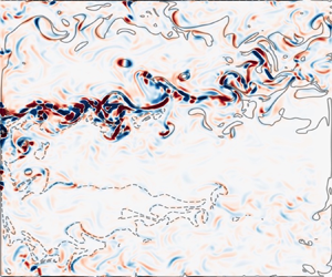
The flow snapshots (figure 1) clearly show two asymmetric gyres of opposite circulation, separated by a strong eastward jet, formed due to the merging western boundary currents and nonlinear eddy interactions. The flow is an idealization of the Gulf Stream in the North Atlantic and Kuroshio in the North Pacific.
Snapshots of the reference solution. Shown are evolving upper-layer fields: (a) PVA, and (b) velocity streamfunction. The colourbars are in dimensionless units, with the length scale equal to the grid interval 7.5 km and velocity scale  $0.01\ \textrm {m}\,\textrm {s}^{-1}$. The positive (red) and negative (blue) values of PVA correspond to the cyclonic and anticyclonic motions, respectively.

For simplicity, from this point onward, we will show our results and analysis mostly for the top and middle layers, since the results for the bottom and middle layers are, usually, qualitatively similar (to be mentioned where they differ).
3. Flow decomposition
In this paper, our first goal is to implement a non-uniform, statistically constrained filtering of the reference flow fields into the large-scale and eddy components. Next, we want to compare the outcome with that of the moving-average filtering based on the baroclinic Rossby deformation radius, and to carry out a comprehensive analysis of the resulting eddy forcing and its relation to the large-scale flow. The generally decomposed streamfunction and PVA fields can be written as
 \begin{equation} \psi (\boldsymbol{x}, t) = \bar{\psi}(\boldsymbol{x}, t) + \psi'(\boldsymbol{x}, t), \quad q (\boldsymbol{x}, t)= \bar{q} (\boldsymbol{x}, t) + q' (\boldsymbol{x}, t) , \end{equation}
where the bars and primes indicate the large-scale and eddy fields, respectively.
Several different methods to obtain (3.1a,b) exist in the literature (e.g. Sagaut Reference Sagaut2006), such as Reynolds decomposition, moving-average filtering, spectral filtering, etc. As discussed in § 1, Reynolds decomposition provides no information about the separated scales in eddy-mean decomposed fields, and the latter two, generally, use a constant filter size for the entire domain – parts of which are evolving on entirely different length/time scales. For this reason, we propose an alternative flow decomposition with spatially-varying filter size across the domain, as discussed below. The application and results from moving-average and spectral filterings are provided in Appendices A and B, respectively.
3.1. Correlation-based decomposition
In this section, we discuss a non-uniform flow decomposition method developed here using local correlation information. This method augments the moving-average filtering while exploiting its advantages. The idea is to filter around each location according to the local length scale of the spatial correlation, as opposed to using a fixed kernel size based on the Rossby deformation radius (for QG this is equivalent to the same kernel size for the whole domain). Below the method is described in detail.
Let us consider the spatio-temporal flow field  $\mathcal {F}$ to be decomposed. For any reference spatial location $\boldsymbol {x_0} = (x_0,y_0)$, we first compute its zero-lag cross-correlation with every other spatial location in the domain (note that every spatial location in $\mathcal {F}$ has a time series) to obtain the corresponding spatial correlation map $C(\boldsymbol {x}_0,\boldsymbol {x})$, and then fit a two-dimensional (2-D) Gaussian function to $|C(\boldsymbol {x}_0,\boldsymbol {x})|$ – the absolute value of the correlation map – to diagnose the effective correlation length scale. The absolute value is used because we are only interested in finding locations with a strong influence on $\boldsymbol {x_0}$; so the sign of the correlation does not matter.
Figure 2(a,d,g,b,e,h) shows correlation maps  $C(\boldsymbol {x}_0,\boldsymbol {x})$ for reference locations $\boldsymbol {x}_0$ in the eastward jet, subpolar gyre and subtropical gyre regions, all in the upper-ocean PVA field (i.e. $\mathcal {F} = q_1$). The correlation maps (figure 2a,d,g) show that the correlations are spatially local in both the jet and the gyre regions and decay exponentially away from the reference locations. A zoomed-in view of the correlations around the reference locations (figure 2b,e,h) further demonstrates that the correlations are nearly isotropic in the subpolar gyre and eastward jet regions but are significantly anisotropic in the subtropical gyre region. For a few reference locations in the subtropical gyre region, we also found the local correlations to be anisotropic at a certain angle (not shown here), whereas those along the western boundary were found to be aligned with the meridional direction, due to the strong western boundary currents. Therefore, to precisely account for the correlation geometry, we fitted a rotated anisotropic Gaussian function positioned at $\boldsymbol {x}_0$ to the full correlation map $|{C(x_0,x)}|$ and determined the effective length scale using the standard deviation of the Gaussian along each axis.
Visualisation of  $|{C(q_1(\boldsymbol {x}_0,\boldsymbol {x}))}|$ contours (a,d,g), its zoomed-in three-dimensional view around the reference location $\boldsymbol {x}_0$ (b,e,h) and the fitted Gaussian function (c,f,i) for three randomly chosen reference locations in the eastward jet (a–c), the subpolar gyre (d–f) and the subtropical gyre (g–i) regions. The entire length of PV anomaly, equal to 15 000 days, is used for computing cross-correlations. The $z$-axis in (b,e,h) and (c,f,i) represents the correlation magnitude and the Gaussian weights, respectively. These have been additionally colour coded to match the contour levels in (a,d,g).

The form of the Gaussian function used is
 \begin{equation} f(x,y; x_0,y_0) = \exp({-}X^{2}/a^{2})\exp({-}Y^{2}/b^{2}) , \end{equation}
where  $X$ and $Y$ are the rotated and translated coordinate axes, given as
 \begin{equation} \begin{bmatrix} X \\ Y \end{bmatrix} = \begin{bmatrix} \cos\theta & \sin\theta \\ -\sin\theta & \cos\theta \end{bmatrix} \begin{bmatrix} x-x_0 \\ y-y_0 , \end{bmatrix} \end{equation}
and  $a$ and $b$ are the standard deviations along them, respectively. Note, that at the reference location $\boldsymbol {x} = \boldsymbol {x}_0$, both $f$ and $C$ are equal to $1$. The fitted Gaussians (figure 2c,f,i) appropriately assign the weights according to the decay of the correlations away from the reference location and adjusts the shape according to the direction and extent of anisotropy. The values of $a$ and $b$ determine the correlation length scale operating along each direction, whereas the overall effective correlation length scale (say, $\mathcal {L}$) can be illustrated by $\mathcal {L} = \sqrt {ab}$. Fitting such a Gaussian function $f$ to the correlation map for each $\boldsymbol {x}_0$ produces the spatial maps $a(\boldsymbol {x};\mathcal {F})$, $b(\boldsymbol {x};\mathcal {F})$, $\theta (\boldsymbol {x}; \mathcal {F})$ and $\mathcal {L}(\boldsymbol {x};\mathcal {F})$ for the given flow field $\mathcal {F}$. The length scale maps $\mathcal {L}(\boldsymbol {x}; \mathcal {F})$ and the inferred anisotropy, computed as $\mathcal {A}(\boldsymbol {x}; \mathcal {F}) = a(\boldsymbol {x}; \mathcal {F})/b(\boldsymbol {x};\mathcal {F})$ (gridpoint-wise division), for the three layers of PVA (i.e. $\mathcal {F} = q_i$, $i = 1,2,3$) are shown in figure 3. We do not show $\theta (\boldsymbol {x}; q_i)$ as it is relatively noisy, and geographical variations in $\theta$ are not particularly interesting.
Maps of correlation length scale  $\mathcal {L}(\boldsymbol {x};q)$ (a,c,e) and the correlation anisotropy $\mathcal {A}(\boldsymbol {x}) = a/b$ (b,d,f) for the three layers of PV anomaly in the top (a,b), middle (c,d) and bottom (e,f) layers. The units of length scale are in km, and the anisotropy estimates are dimensionless.

Significant geographical variations in  $\mathcal {L}(\boldsymbol {x}; q_i)$ attest multiscale and inhomogeneous properties of the mesoscale turbulence (figure 3a,c,e). In the upper ocean (figure 3a), the eastward jet region exhibits mean $\mathcal {L}(q_1)$ equal to 91 km, which is comparable to the filtering based on $2.25 Rd_1$, whereas the subpolar and subtropical gyres have mean correlation length scales equal to $108$ and 133 km, respectively. The mean and median length scale for the entire domain is roughly 105 km, i.e. slightly higher than $2.5 Rd_1$. A region of even larger $\mathcal {L}(\boldsymbol {x})$ exists in the centre of the basin in the middle layer (figure 3c), where typical $\mathcal {L}$ values are 250–500 km. This is because this part of the basin is dominated by a large-scale interdecadal variability pattern with long-range correlations (figure 4). Large differences between the correlation length scales at the two layers infer the need to emulate eddies as horizontally and vertically inhomogeneous, and multiscale entities. In the bottom layer (figure 3e), $\mathcal {L}(\boldsymbol {x})$ is relatively short along the western boundary and long along the eastern one (south of the eastward jet). This is consistent with the prevalence of small-scale eddies in the former region and long waves radiating from the eastern boundary in the latter one.
The empirical orthogonal function (EOF) representing the large-scale interdecadal variability in  $q_2$, responsible for producing large $\mathcal {L}$ in the middle of the domain (see figure 3c). The decorrelation time scale for this pattern is roughly $16.7$ years, as obtained from the temporal autocorrelation of its principal component. A stripe of $30$ grid points is removed from all four boundaries of $q_2$ before its EOF decomposition to get this as the first EOF; otherwise, boundary trapped eddies dominate a large chunk of leading EOFs, thus making it harder to detect this variability. Units are non-dimensional.

The  $\mathcal {A}(\boldsymbol {x};q_i)$ maps (figure 3b,d,f) infer that the correlations are mostly anisotropic in the large-length-scale regions, except near the western and eastern boundaries, where it is inherently stretched in the meridional direction (i.e. $a/b < 1$). Anisotropy along the lateral boundaries is due to the strong western boundary current and zonal radiation from the eastern boundary (it is more intense in deep layers). The $\mathcal {A}(\boldsymbol {x})$ values for the top-layer PV anomaly (figure 3b) also infer that the correlations in the jet region are nearly isotropic – mainly due to the rich eddy activities in this region leading to localised coherent isotropic structures. However, in the deeper layers (figure 3d,f), as the eastward jet gets weaker, the flow around it becomes more anisotropically correlated with its neighbouring locations.
The length scale and anisotropy maps together reveal the complex and multiscale nature of the flow, and suggest that a fixed-size kernel can substantially underfilter or overfilter eddies depending on the location; therefore, a differential filter size over the domain is justified. For practical applications, correlation length scales are to be determined from observational data and, in some cases, from eddy-resolving model solutions. Note that the CBD provides additional flexibility of imbuing temporal dependency in the correlation length scales by employing time-lagged correlation (i.e.  $C(\boldsymbol {x}_0,\boldsymbol {x}; \tau )$, where $\tau$ is the anticipated time scale of variation in the length scales) instead of instantaneous correlation ( $C(\boldsymbol {x}_0,\boldsymbol {x}$)) discussed here.
We filtered each spatial location of the PVA fields using a rotated anisotropic Gaussian kernel as defined in (3.2), with the diagnosed parameters  $a, b$ and $\theta$. This can be expressed as
 \begin{equation} \bar{q}(x_i,y_j, t) = \sum_{i'} \sum_{j'} G(x_{i'},y_{j'}; x_i,y_j) q(x_{i'},y_{j'},t); \quad 1 \leq i',j' \leq 513 , \end{equation}
where  $G$ is the normalized Gaussian kernel,
 \begin{equation} G(x_{i'},y_{j'}; x_i,y_j) = \dfrac{f(x_{i'},y_{j'}; x_i,y_j)}{A_f}, \end{equation}
and  $A_f = \sum _{i'}\sum _{j'} f(x_{i'},y_{j'}; x_i,y_j)\equiv {\rm \pi}ab$ is the sum of the Gaussian weights per (3.2). Note that only the grid points within the Gaussian ellipse would contribute significantly in (3.4) because the Gaussian weights decay exponentially with distance from the ellipse centre.
Using (3.4) and (3.1a,b), the large- and small-scale components of PVA fields were obtained for each layer, and the corresponding streamfunctions were obtained by inversion of (2.4) (figure 5). On comparing these eddy fields with the corresponding full flow snapshots (figure 1), we see (especially for  $\psi _1$) vigorous eddy activity along the eastward jet extension and near boundaries. Note that the process can be reversed, i.e. by filtering streamfunction fields first, then by obtaining PVA using (2.4); however, we found that this algorithm generates discontinuities in PVA upon the differentiation (note that the inversion is intrinsically a smoother operation).
Snapshots of (a)  $\bar {q}_1$, (b) $q'_1$, (c) $\bar {\psi }_1$, (d) $\psi '_1$ obtained using the CBD method. (a,b) show that gyres and the eastward jet are well captured by the large-scale flow component; (c,d) shows vigorous eddies all over the basin but with the largest concentration in the eastward jet region and around the boundaries. The colour scales are in non-dimensional units.

4. Results
4.1. CBD eddy forcing
In the following, we analyse eddy feedbacks on the large-scale flow by considering eddy forcing, which is argued to play an important role in the maintenance of large-scale flow features such as the eastward jet and its adjacent recirculation zones (Nadiga Reference Nadiga2008; Shevchenko & Berloff Reference Shevchenko and Berloff2016). Revealing the essential and poorly understood statistical characteristics of the eddy forcing is our next goal. This information should help to improve statistical eddy models by constraining them to preserve these characteristics.
The eddy forcing is obtained by substituting the decomposed flow (3.1a,b) into the governing equation (2.1), and by rewriting it as the evolution equation for the large-scale component as (illustrated only for the top layer but applicable for each layer)
 \begin{equation} \frac{\partial{(\bar{q}_1 + q_1')}}{\partial t} + J(\bar{\psi}_1 + \psi_1',\bar{q}_1 + q_1') + \beta\frac{\partial {(\bar{\psi}_1 + \psi_1')}}{\partial x} = \frac{1}{\rho_1H_1} W(x,y) + \nu\nabla^{4}(\bar{\psi}_1 + \psi_1') , \end{equation}
which on rearrangement gives
 \begin{equation} \frac{\partial\bar{q}_1}{\partial t} + J(\bar{\psi}_1,\bar{q}_1) + \beta\frac{\partial \bar{\psi}_1 }{\partial x} = \mathcal{H}(\bar{q}_1,\bar{\psi}_1) + \mathcal{I}(q_1',\psi_1') + \mathcal{N}(\bar{q}_1,\bar{\psi}_1,q_1',\psi_1') , \end{equation}
where
 \begin{gather} \mathcal{H}(\bar{q}_1,\bar{\psi}_1) = \frac{1}{\rho_1H_1} W(x,y) + \nu\nabla^{4}\bar{\psi}_1, \end{gather}
 \begin{gather}\mathcal{I}(q_1',\psi_1') ={-} \frac{\partial q'_1}{\partial t} - \beta\frac{\partial \psi_1' }{\partial x}, \end{gather}
 \begin{gather}\mathcal{N}(\bar{q}_1,\bar{\psi}_1,q_1',\psi_1') ={-} J(\psi_1',\bar{q}_1) - J(\bar{\psi}_1,q_1') - J(\psi_1',q_1') . \end{gather}
Clearly, the final expression (4.2) provides both linear  $\mathcal {I}(q_1',\psi _1')$ and nonlinear $\mathcal {N}(\bar {q}_1,\bar {\psi }_1,q_1',\psi _1')$ terms expressing the feedbacks from the eddy- to large-scale fields. The linear term was found to be much smaller than the nonlinear one (also seen by Ryzhov et al. Reference Ryzhov, Kondrashov, Agarwal and Berloff2019). Therefore, we approximated the eddy forcing by the nonlinear term $\mathcal {N}$, i.e.:
 \begin{align} E_i(x,y;t) & ={-} [J(\bar{\psi}_i,q_i') + J(\psi_i',\bar{q}_i) + J(\psi_i',q_i')] \end{align}
 \begin{align} & ={-} [J(\psi_i, q_i) - J(\bar{\psi}_i,\bar{q}_i)] , \end{align}
where  $i$ is the layer index, overbar indicates the large-scale component and prime indicates the eddy component; the others are the full fields. The eddy forcing can also be written in the flux divergence form as
 \begin{equation} E_i(x,y;t) ={-} [\boldsymbol{\nabla} \boldsymbol{\cdot} \boldsymbol{u}_iq_i - \boldsymbol{\nabla} \boldsymbol{\cdot} \boldsymbol{\bar{u}}_i\bar{q}_i], \end{equation}
where  $\boldsymbol {u}$ is the non-divergent geostrophic velocity. Note that this is different from the commonly used large-eddy simulation (LES)-based definition of instantaneous eddy forcing:
 \begin{equation} E_i^{LES}(x,y;t) ={-} [\boldsymbol{\nabla} \boldsymbol{\cdot} \overline{\boldsymbol{u}_i q_i} - \boldsymbol{\nabla} \boldsymbol{\cdot} \boldsymbol{\bar{u}}_i \bar{q}_i] . \end{equation}
 The differences between the expressions are as follows. First, (4.6) is only applicable to the filtering methods which commute with partial derivatives (otherwise  $\boldsymbol {\nabla } \boldsymbol {\cdot } \overline {\boldsymbol {u}_i q_i}$ becomes $\overline {\boldsymbol {\nabla } \boldsymbol {\cdot } \boldsymbol {u}_i q_i}$). So, it does not hold for the CBD, as it involves a spatially varying filtering kernel and does not commute with spatial derivatives. However, (4.5) is more flexible and holds for all filtering methods, as it is obtained by direct substitution of the filtered fields into the governing equation. Second, for $E^{LES}$, we need the same characteristic length scales of $\boldsymbol {u}q$, $\boldsymbol {u}$ and $q$, but they are unlikely to be the same. Because we cannot filter the governing equations using multiple filters, the whole process is either infeasible or leads to inconsistent results if an approximate length scale is used for all three. In contrast, $E$ is easier to generalize for filtering based on variable kernel sizes and shapes. Moreover, it only involves the filtering of $\boldsymbol {u}$ and $q$, which are connected by the PV inversion. Third, the dynamics of $E$ has clearly interpreted nonlinear advection terms, whereas the nonlinear terms in $E^{LES}$ are harder to interpret (e.g. they are not advection) because they involve double filterings.
We diagnosed  $E$ from the data using the energy and enstrophy conserving Arakawa's Jacobian discretization (Arakawa Reference Arakawa1966). From the spatio-temporal statistics of $E$, it is clear that the eddy forcing is most intense in the upper-ocean eastward jet region, and it weakens away from it and becomes more homogeneously distributed with depth (figure 6a,b). The time-mean $E_1$ (figure 6c) has very small values in the jet region and even less elsewhere. By decomposing $E_1$ into its time-mean ( $\langle E_1 \rangle (x,y$)) and transient ( $E_1'(x,y,t$)) components, we found that in the eastward jet region the standard deviation of $E_1'$ is an order of magnitude larger than $\langle E_1 \rangle$ (figure 6d), thus, suggesting that $E_1'(x,y,t)$ dominates over $\langle E_1 \rangle (x,y)$.
Patterns of the instantaneous eddy forcing  $E$ from CBD for the (a) top and the (b) middle isopycnal layers. The colourbars are in non-dimensional units. Clearly, the eddy forcing is concentrated in the upper-ocean eastward jet region. (c) Time-mean and (d) standard deviation of $E_1$. The time-mean field is weaker by an order of magnitude, suggesting that the eddy forcing feedback is mostly due to the fluctuations, which are most pronounced in the jet region.

To characterize the correlation length scales of the eddy forcing, we used the Gaussian fitting method described in § 3.1 and obtained the length scale map  $\mathcal {L}(\boldsymbol {x};E_i)$ and the anisotropy map $\mathcal {A}(\boldsymbol {x};E_i)$. The $\mathcal {L}(\boldsymbol {x}; E_1)$ map (figure 7a) shows approximately 20 km long correlation scales around the eastward jet and in the subpolar gyre region, but they are approximately $5$ km longer to the south of the jet and towards the eastern boundary. The latter region of relatively long correlation length scales extends out with depth (figure 7b), but the eastward jet region still retains short $\mathcal {L}$ values. This shows that the eddy forcing is the most tightly correlated where it is the most intense. Furthermore, the ratio of the $\mathcal {L}$ values for the PVA and eddy forcing fields shows that, on average, the eddy forcing $\mathcal {L}$ values are approximately $5$ times smaller (figure 3a,c,e) than the PVA ones, both globally and around the eastward jet. Since one needs at least two grid intervals to approximate a length scale, this implies that at least 10 grid intervals are needed to represent an eddy forcing dynamically. The eddy forcing $E$ is expected to be dominated by small spatial scales as all the computations are performed on the fine grid and that it is a triply differentiated field (in streamfunction) involving the eddy fields. Small-scale dominance of the eddy forcing is also true for the standard LES-type eddy forcing, e.g. the one derived by Mana & Zanna (Reference Mana and Zanna2014) using a similar QG ocean model. Furthermore, the $\mathcal {A}(\boldsymbol {x}; E_1)$ map (figure 7c) implies that the eddy forcing correlations are nearly isotropic in the entire domain (mean $\mathcal {A}(\boldsymbol {x}) = 1.1$), but relatively more so in the subpolar gyre (mean $\mathcal {A}(\boldsymbol {x}) = 1$) than in the eastward jet and the subtropical gyre region (mean $\mathcal {A}(\boldsymbol {x}) = 1.2$).
Correlation length scale maps  $\mathcal {L}(\boldsymbol {x})$ (in km) for the CBD-decomposed outputs: (a) $E_1$ and (b) $E_2$, (c) the anisotropy map $\mathcal {A}(\boldsymbol {x};E_1)$ and (d) the time scale map (in days) for $E_1$. Relative to PVAs, the eddy forcing is characterized by significantly smaller length and time scales (compare with figure 3(a,c,e); the time scale map for PVA is not shown for brevity).

To characterize the eddy forcing further, we diagnosed the temporal scale for each grid point – defined as the lag at which the corresponding autocorrelation drops by a factor of  $\exp$ from the zero-lag value – and analysed the resulting correlation time scale map. The fast evolving nature of the eddy forcing is visible in its top-layer time scale plot (figure 7d). In particular, the eastward jet region is dominated by the shortest correlation time scales and is characterized by the average correlation time scale of $1$ day, which is approximately 3 times shorter than in the interior gyres and is approximately $25$ times shorter than PVA time correlations in the eastward jet region (not shown for brevity). Locally, eddy forcing on the north and south flanks of the eastward jet has correlation time scales of approximately $1.8$ and $3.5$ days, respectively, whereas its basin-averaged value is approximately $2.7$ days. Overall, the spatio-temporal correlation study of the eddy forcing suggest that it can be modelled as a stochastic field with short spatio-temporal correlations in the regions where it is most intense.
In comparison,  $q_1$ yields correlation time scales of $25$ days in the eastward jet and ${\sim}10^{4}$ days in the gyre regions (not shown). The corresponding basin averaged correlation time is ${\sim}9500$ days, which is more than $3500$ times that for the eddy forcing – annotating the differences between the two very different yet interacting flow fields.
Therefore, we learned that (i) the eddy forcing is characterized by grid-scale level correlation in space and  $O(1)$ days correlation in the temporal domain – much smaller than the induced PVA field, (ii) the eddy forcing is least spatially correlated where it is the most intense – the jet eastward region, and (iii) the transient component of the eddy forcing is more dominant than its time-mean. How exactly can this small-scale and highly transient eddy forcing feed back on the much larger and slower evolving large-scale flow features? Studying this process is the main subject of the next section.
4.2. Product integral analysis
Next, we intend to study the dynamical characteristics of the eddy forcing and the induced large-scale flow, and quantify their possible interactions using a suitable metric. The goal here is to illuminate the eddy backscatter mechanism, which supports the eastward jet and its adjacent recirculation zones, and, thus, is characterized statistically by a positive correlation between the transient eddy forcing and large-scale flow response. To achieve this, we used an approach based on analysing the product integral  $I(t)$, defined instantaneously as the spatial integral of the point-wise (Hadamard) product $\odot$ of two standardized snapshots (i.e. point-wise subtracting the time-mean and dividing by the standard deviation) from flow fields, say, $\mathcal {F}_1$ and $\mathcal {F}_2$:
 \begin{equation} I(t) = \frac{1}{A} \iint _\varOmega { \hat{\mathcal{F}}_1(x,y; t) \odot \hat{\mathcal{F}}_2(x,y; t) \,\mathrm{d} {x} \,\mathrm{d} {y} } \, , \end{equation}
where  $A$ is area of the domain $\varOmega$.
We calculated  $I(t)$ for $\mathcal {F}_1 = \bar {q}_1$ and $\mathcal {F}_2 = E_1$. The resulting instantaneous product integral was found to have mixed positive and negative values with a negative time-mean (figure 8a), but this value should be treated cautiously, as the two flow variables (i.e. $\bar {q}_1$ and $E_1$) evolve on very different space and time scales (as shown in §§ 4.1 and 3.1), and the flow response to eddy forcing may accumulate over time rather than being instantaneous. Therefore, a time-lagged extension of (4.7) was applied to get more insight into the relation between the eddy forcing and the large-scale flow response after time lag $\tau$, i.e.
 \begin{equation} I(t,\tau) = \frac{1}{A} \iint _\varOmega { \hat{\mathcal{F}}_1(x,y; t + \tau) \odot \hat{\mathcal{F}}_2(x,y; t) \,\mathrm{d} {x} \,\mathrm{d} {y} } , \end{equation}
with  $\mathcal {F}_1 = \bar {q}_1$ and $\mathcal {F}_2 = E_1$. The time-lagged $I(t,\tau )$ curve with $\tau =1$ day (figure 8b) clearly shows a positive feedback from the eddy forcing to the flow response, and, therefore, suggests the eddy backscatter mechanism. Such a positive time-lagged correlation between $E_1$ and $\bar {q}_1$ is not obvious, because (i) there are other terms in the governing equation, and (ii) no such lagged correlation exists for white-noise forcing in the same governing equation. By considering the time-lagged relation, we advanced the results of Berloff (Reference Berloff2018) where only zero lag was considered, and the resulting product integral (between large-scale PV anomaly and eddy forcing) was found to be positive due to the excessively large filter size – equal to $5Rd_1$. Therefore, the correct conclusion was based on the less general diagnostics. Here, our time-lagged detection of the main eddy backscatter characteristics is a lot more solid and substantially reinforces the previous conclusions. Dynamical interpretation of this result is that the flow adjustment due to the eddy feedback happens not instantly but with some delay. To see if the eastward jet region is particularly susceptible to the eddy backscatter, we repeated the analyses only for the eastward jet region, but the outcome was the same.
Product integral  $I(t)$ between $\bar {q}_1$ and coarse-grained $E_1$ for (a) $\tau =0$ and (b) $\tau =1$ day. The red lines indicate $I(t)=0$, which is used to define instants of positive $I$. The curve in (b) illustrates presence of the underlying eddy backscatter, as it shows positive correlation between the eddy forcing and the large-scale flow response for most of the time.

We considered values of  $\tau$ up to $20$ days, to find that the time-mean product integral $\langle I(t,\tau ) \rangle = (1/T) \int _0^{T} I(t, \tau ) \,\mathrm {d} {t}$ – or spatial time-lagged correlation – increases with $\tau$ monotonically, peaks at around $9$ days and then decays monotonically towards zero (figure 9a). The standard deviation of $\langle I(t,\tau ) \rangle$ is also very small for small lags but increases thereafter, reaching the maximum at $\tau =9$ days. Note that although the values of $\langle I(t,\tau ) \rangle$ are small, on randomizing $\widehat {E_1}$ in (4.8) we obtained three orders of magnitude smaller values, which inferred the significance of the illuminated spatio-temporal correlation between the two dynamically complex and structurally very different flow fields that were shown to evolve on different space and time scales. We refer to the time lag of the maximum correlation as the backscatter response time scale. Using a few other normalization techniques, such as $L_2$ norm, scaling between $[0,1]$, etc., we also proved the insensitivity of the $\tau$-dependence curve to the chosen normalization.
Plot of the time-lag dependence of the product integral correlation between coarse-grained  $E_1$ and $\bar {q}_1$ (a) for the full domain and (b) for the eastward jet region. The jet region was defined over the locations where the standard deviation of $E_1$ is more than 50 (in non-dimensional units). The two dashed lines indicate $I(t)$ values within two standard deviations from the mean. Both (a,b) characterize the eddy backscatter and its response time scale.

We also analysed the  $\langle I(t,\tau ) \rangle$ curve for the eastward jet region (figure 9b) and there are a few key differences to note: (i) the zero-time-lag correlation is small but positive in the jet region; (ii) the backscatter response time scale is almost half for the jet region, which proves the insignificance of long memory effects of the eddy feedback over there; (iii) for each $\tau$ the standard deviation of $I(t,\tau )$ is higher for the jet region than on average, thus indicating more multiscale nonlinear interactions.
Additionally, we explored the time-lagged product integral correlation between  $\mathcal {F}_1 = \mathrm {d} \bar {q}_1/\mathrm {d} t$ and $\mathcal {F}_2 = E_1$ and obtained positive instantaneous correlation between the two, which is also the maximum; and the correlation decreased monotonically with the lag. The magnitude of the correlation was also found to be somewhat higher in the eastward jet region. Together with the product integrals between $E_1$ and $\bar {q}_1$, it suggests that the positive (negative) part of the transient eddy forcing instantaneously drives the tendency of positive (negative) flow anomalies, and this effect manifests itself in the induced flow field after a definite time scale – different for the jet and the gyre regions. Note that this conclusion cannot be drawn only using the positive correlation seen between $E_1$ and $\partial \bar {q}_1/\mathrm {d} t$, as feedback between opposite polarities of $E_1$ and $\bar {q}_1$ anomalies is also possible under such a positive correlation.
Next, we studied the global and jet-regional  $\langle I(t,\tau ) \rangle$ curves for $\bar {q}_1$ and $E_1$ obtained using the fixed-size moving-average decomposition method with three filter sizes: $11$,
$11$,  $20$ and $40$ grid intervals (hereafter referred to as F11, F20 and F40), which correspond to $82.5$ km, $150$ km and $300$ km, respectively (in terms of $Rd_1$, these are approximately $2Rd_1$, $3.75Rd_1$ and $7.5Rd_1$). Note, that F11 is the most obvious choice for a filter size based on $Rd_1$ when using the fixed-size moving average method; F20 and F40 are among other reasonable choices of larger filter sizes. Additionally, the mean length scale diagnosed for the top-layer PVA using CBD (figure 3a) is approximately equal to $105$ km and, therefore, is in between the F11 and F20 filter sizes. For the full field correlation plot (figure 10a), the overall shape of the curve was the same for all cases, but F11 and CBD outcomes resembled each other the most; especially up to the backscatter response time scale, beyond which F11 correlations decayed faster. Overall, the CBD produced equal or higher correlations than F11, at all time lags. However, the outcomes were very different for the eastward jet region (figure 10b), as the CBD-produced eddy forcing showed a much higher correlation (with $\bar {q}_1$) than F11, and this correlation was strongest around the backscatter time scale, which was roughly equal to $5$ days. In effect, the CBD-produced eddy forcing yields a stronger feedback on to the large-scale flow field in the eastward jet region, where the backscatter is most pronounced. On the other hand, F20 and F40 filtering kernels result in larger backscatter response time scales, both globally and in the eastward jet region. In general, the time scale increases with an increase in moving-average filter size, whereas the amplitude of correlation goes down. The full-domain zero-lag correlation is also small and positive for F20 and F40 filters, contrary to CBD and F11. A similar $\langle I(t,\tau ) \rangle$ analysis for the interior gyres showed small differences between the F11 and CBD results, whereas the F20 and F40 ones differed vastly from them. For the subtropical gyre, F11 and CBD correlation curves resembled those for the full field, but, in the subpolar gyre, the F11 correlations remained generally lower than the CBD ones.
Comparison of the correlation curves (between coarse-grained  $E_1$ and $\bar {q}_1$) from CBD and the three moving-average cases (F11, F20, F40) for (a) the full domain and (b) the eastward jet region. As the moving-average filter size increases, the correlation curves becomes flatter, their correlation amplitudes decrease, and the backscatter time scale information is lost. Also, CBD captures the highest correlation in the jet region, which indicates the backscatter in a most pronounced way.

Overall, this suggests that the performance of moving average filters is critically sensitive to the choice of filter size, and looking for and developing a less subjective filtering approach is totally justified. We also tried including a spectral filtering approach in the comparison list but obtained highly noisy and inconsistent decomposed fields for  $q_1$ – due to the non-locality of coherent vortices and the eastward jet region in the spectral domain (discussed and shown in Appendices B).
Therefore, considering the lack of knowledge about the optimal filter sizes for eddy-/large-scale decompositions, CBD provides a powerful alternative with no explicit hyperparameter dependence of its characteristics. Another advantage of CBD is its usefulness for the unstructured grid systems, where uniform moving average filtering can cause significant distortions. In the next section, we investigate the dynamical relevance of CBD eddy fields by using them to augment a low-resolution non-eddy-resolving model solution. In the future, we will exploit the comprehensive study done here to build low-order data-driven models for CBD eddy fields and use them for such low-resolution model augmentations.
4.3. Augmentation of the coarse-resolution solution
In this section, we test the dynamical relevance of the CBD-produced eddy fields by applying an augmentation procedure of the corresponding coarse-resolution model and compare the augmented solution against the high-resolution reference. The augmentation procedure is comprehensively introduced by Ryzhov et al. (Reference Ryzhov, Kondrashov, Agarwal, McWilliams and Berloff2020). It involves supplying small-scale fields into the coarse-resolution model during its run, thus correcting its solution interactively as (valid for all three layers)
 \begin{equation} \frac{\partial q_c}{\partial t} + J(\psi_c,q_c) + \beta\frac{\partial \psi_c}{\partial x} = \mathcal{H}(\psi_c,q_c) + \mathcal{E}(\psi_c,q_c,\psi',q') , \end{equation}
where the subscript  $c$ denotes coarse-resolution (or low-resolution) solutions; $\mathcal {H}$ represents all terms involving the coarse-resolution solutions $\psi _c, q_c$; and $\mathcal {E}$ presents the interactive eddy forcing computed using the coarse-resolution solutions and the supplied eddy fields $\psi ', q'$ from the eddy-/large-scale decomposition of the high-resolution solution (the eddy fields are coarse grained to the available coarse resolution before adding). Note that the expression (4.9) is analogous to (4.2), but the coarse-resolution solutions $q_c$ and $\psi _c$ are not the same as $\bar {q}$ and $\bar {\psi }$ – this is a known problem in model augmentation and parametrization in general and addressing it is outside the scope of the paper. A similar coarse-resolution model augmentation technique can also be applied using the eddy forcing history $E$ (4.4a) itself (Ryzhov et al. Reference Ryzhov, Kondrashov, Agarwal and Berloff2019). However, the corresponding off-line eddy forcing history additionally involves the high-resolution (‘true’) large-scale fields, which is more demanding in terms of external data availability as compared with using only the high-resolution eddy field in the on-line eddy forcing computation. Moreover, our approach allows for the interactive (hence part of the solution) feedback from the eddy component to the large-scale one.
We considered an eddy permitting coarse-resolution model with a grid resolution of  $129\times 129$, compared with an eddy-resolving $513\times 513$ for the high-resolution model. The coarse-resolution model by itself fails to produce the eastward jet (which is mostly eddy-driven) and its adjacent recirculation zones – attested both by the flow snapshot (figure 11a) and the temporal standard deviation (figure 11b); conversely, the high-resolution solution produces a pronounced eastward jet separating the two gyres (figure 11c,d).
Comparison of the coarse-resolution, high-resolution, F11- and CBD-augmented model solution snapshots (panels a,c,e,g) of the top-layer PV anomaly and their standard deviations (panels b,d,f,h, respectively) for  $15\,000$ days of data. Starting from the top, the four rows belong to coarse-, high-resolution, F11- and CBD-augmented model solutions, respectively.

For coarse-resolution augmentation, we (i) decomposed the high-resolution PVA into its large- and small-scale components (as described in § 3.1), followed by their inversions to get the corresponding streamfunctions, (ii) coarse-grained the eddy streamfunction to a  $129\times 129$ grid resolution by applying local averaging over $4$ by $4$ high-resolution grid intervals (the difference between the high- and coarse-resolution counterparts), (iii) obtained coarse-grained eddy PVA using the vorticity–streamfunction relationship (2.4), and finally (iv) added both eddy fields to the coarse-resolution model, as described in (4.9), through on-line calculation of eddy forcing at each time step (note that the coarse-grid $\psi '$ and $q'$ can also be obtained by coarse-graining $q'$ directly in step (ii) and inverting it to get $\psi '$ at the same resolution.). We spun up the coarse-resolution model – until it reached its statistically equilibrated state – before integrating it for an additional $15\,000$ days of the available external small-scale fields, and comparing its statistical properties with those of the coarse- and high-resolution solutions (of similar time length). The augmentation is performed for both F11- and CBD-produced eddy fields, as the two filters provide nearly similar product integral correlations, as seen in the previous section. For both, the components of the eddy forcing are the corresponding coarse-resolution solutions and the externally supplied small-scale (eddy) fields.
The augmented flow snapshot for F11 (figure 11e) shows poor jet reconstruction and weak eddy activities around it, whereas the CBD augmented solution (figure 11g) shows considerably more eddying features and a stronger eastward and also meandering jet, with all these features being closer to the reference ‘truth’ – the high-resolution solution. The standard deviation of the augmented solutions for the two methods (figure 11f,h) further distinguishes between the induced variabilities around the jet region. The CBD produces much more variability around the jet, with more pronounced eastward extension of it, as compared with F11, which yields marginal improvement relative to the coarse-resolution model solution (figure 11b). However, there are still some notable differences between the standard deviation of the CBD-augmented solution and the high-resolution reference flow, as the latter shows even higher values near the eastward jet. This suggests that the evolving states of the CBD augmented model lie on a different attractor than the high-resolution reference (similar to that observed by Nadiga & Livescu Reference Nadiga and Livescu2007). Consequently, this means that the supplied eddy fields operate differently than the corresponding perfect eddy field – i.e. those extracted from a perfect decomposition with  $q_c = \bar {q}$ and the same initial condition for both high-resolution and the augmented model. Here, the eddy fields get quickly decorrelated from the coarse-grid model solution they are augmenting. This inherent property of the eddy fields makes them suitable for stochastic treatment to develop parametrizations while also accounting for the effects of initial condition perturbations.
The reason behind poor augmentation by the F11 eddy field is the weak interactive eddy forcing generated in conjunction with  $\psi _c$ and $q_c$ (figure 12a). In comparison, the CBD eddy forcing (figure 12b) is much stronger and more eastward-extended than its F11 counterpart, thereby providing a much better augmentation. To understand the impact of this discrepancy in the eddy forcing on eddy backscatter, we analysed the corresponding product integral correlations between the augmented PVA and the online eddy forcing $\mathcal {E}$ (figure 12c). The results suggest that both F11 and CBD eddy forcings possess similar correlations with the induced PV anomaly, and the same backscatter time scale; the CBD eddy forcing is only marginally highly correlated with its induced PVA at short time-lags (1–10 days). Recall that, even in § 4.2 (figure 10a) we found the product integral correlation (i.e. backscatter) characteristics of F11 and CBD to be nearly the same; the current results verify them for online eddy forcing. However, on analysing the corresponding covariances – obtained using (4.8) but without normalizing the two flow fields by their standard deviations – we found an order of magnitude of difference between F11 and CBD (figure 12d). The correlation and covariance results together suggest that, although the F11 eddies feedback similarly on the induced PV anomalies, the low magnitude of its eddy forcing fails to deliver a significant jet reconstruction and, therefore, the resulting induced PVA is also weak compared with CBD, which shows significantly strong variabilities around the jet. This collective intensity of the eddy forcing and the induced dynamical response is captured in the covariance magnitude, which is an order of magnitude smaller for F11 than CBD. The contribution of the eddy forcing intensity alone on the covariance magnitude can be quantified using semi-covariance – i.e. those obtained using (4.8) with normalized induced PVA but un-normalized eddy forcing. Such a semi-covariance magnitude is also significantly high for CBD compared with F11 (not shown). It may sound sensible to use a larger filter size instead of F11 to enhance the eddy forcing strength and thereby improve the jet characteristics, but it is already shown in § 4.1 that such big filter sizes (e.g. F20, F40) lead to poor backscatter; therefore, this is not an option.
Comparison of the standard deviations of the online eddy forcing computed using (a) F11 and (b) CBD eddy fields for the coarse-resolution solution augmentation. (c) The product integral correlations between the augmented PV anomaly and the corresponding eddy forcings for F11 and CBD decompositions. (d) Same as (c) but covariance. The covariance is obtained by using (4.8) but without normalizing the two flow fields by their standard deviations.

Finally, we performed Fourier spectral analysis of the basin-average potential energy time series, given as
 \begin{equation} P(t) = \frac{1}{2} \sum_{i=2}^{3} \frac{H_i (\delta_{i2} S_{i2} + \delta_{i3} S_i)}{V} \iint _{\varOmega} (\psi_i - \psi_{i-1})^{2} \, \mathrm{d} y \, \mathrm{d} x, \end{equation}
where  $S_{ij}$ and $S_i$ are the stratification coefficients, $H_i$ is the height of the $i$th isopycnal and $V = L_x L_y H$ is the volume of the basin with $H = \sum _{i=1}^{3} H_i$. We computed $P(t)$ for both F11 and CBD solutions, and compared them against those for the coarse- and high-resolution solutions. Total available potential energy is an essential global characteristic of the solutions, and here we seek the manifestation of the intrinsic large-scale low-frequency variabilities (LFVs), which are interrelated to other large-scale flow features, such as the eastward jet extension and its adjacent recirculation zones (Berloff, Hogg & Dewar Reference Berloff, Hogg and Dewar2007b). Berloff et al. (Reference Berloff, Dewar, Kravtsov and McWilliams2007a) also showed that such LFVs feedback on the atmosphere in ocean–atmosphere coupled models and, therefore, are of significant dynamical importance. At high spatial resolutions, the reference flow regime possesses broadband energy modulations around $17$ years variability, i.e. at a frequency value of $0.06$ years $^{-1}$, whereas the coarse-resolution solution fails to simulate this, because of the poorly resolved eddies (figure 13). Therefore, feeding in dynamically consistent eddy statistics is necessary for strengthening the eastward jet and the associated LFV. The Fourier spectra of the total potential energy (figure 13) for CBD suggests the presence of pronounced broadband LFV, as contrasted to F11, with an order of magnitude difference between the corresponding spectral powers. This is a remarkable characteristic of CBD, as earlier, Ryzhov et al. (Reference Ryzhov, Kondrashov, Agarwal, McWilliams and Berloff2020) showed that imbuing LFVs in the augmented solutions by merely feeding the eddies from fixed-size moving average filtering is hardly possible (even for larger filter sizes, e.g. F20). Reconstruction of the LFV is a significant advantage of CBD, and it additionally proves that the decomposed eddy fields interact with the coarse-resolution solutions in a more dynamically correct sense, so that these solutions closer resemble the high-resolution reference flow regime.
Comparison of the power spectral density (PSD) estimates for coarse-resolution, high-resolution, F11- and CBD-augmented solutions. The PSD is computed using the robust multitaper method, as introduced by Percival et al. (Reference Percival1993).

Overall, our study confirmed that augmentation of the model restored the key large-scale flow features (e.g. the eastward jet) and the important LFV in the coarse-resolution solutions. This was made possible by plainly supplying the eddy fields extracted from a high-resolution solution. But this requires a more objective and precise scale separation method, such as those based on actual operating correlation length scales, their anisotropy and their orientation. The success of CBD encourages us to look for efficient statistical emulators to model the corresponding eddy fields and supply them instead of the true eddy fields, but this is left for future work.
5. Conclusions and discussion
This study aims to develop methods and approaches for exploring the properties of oceanic mesoscale eddies, study their dynamical feedbacks on the underlying large-scale flow and use them to augment non-eddy-resolving ocean model solutions. For this purpose, we used an eddy-resolving, double-gyre, classical quasigeostrophic model solution as an idealized representation of the North Atlantic or North Pacific ocean circulations. Defining and understanding fundamental statistical and dynamical properties of the oceanic mesoscale eddies is important for their parametrization in the non-eddy-resolving and eddy-permitting oceanic general circulation models. In this regard, dealing with the correct and relevant eddy statistics is crucial. The existing flow decomposition (i.e. scale separation) methods, such as the Reynolds decomposition, moving average, etc., which filter out an eddy component from the flow field, proved their usefulness but also have significant shortcomings. While the classical Reynolds decomposition does not incorporate any scale information, the moving-average decomposition imposes a filter size that is fixed across the domain and based on some scale assumption, such as assuming that the eddies operate on the first baroclinic Rossby deformation radius everywhere. Such an assumption is not necessarily accurate given the intrinsically multiscale nature of the eddies and of their underlying large-scale flow field. Another common strategy is to choose the filter size based on the resolution of the coarse-grid model, which needs eddy parametrizations. However, a nominally resolved flow feature in a dynamical model is not necessarily dynamically resolved with needed accuracy, and there is a broad ‘grey zone’ of partially resolved scales that further complicates the choice of filter size. This motivated us to explore a range of other filtering possibilities and look at the underlying differences to develop a better understanding of the eddy scales. Here, we have proposed a correlation-based decomposition (CBD) method which decomposes the flow using the concept of a differential filter size varying across the domain and based on the local correlation length scale diagnosed from the spatial correlation maps. In other words, instead of imposing an a priori assumption, we let the flow correlation statistics make its own decision on the filtering scale, which is now allowed to vary across the domain and be independent of the Rossby radius. We extracted the spatially varying length scale statistics using a Gaussian-shape fit to the local correlation maps, which additionally infers anisotropy and orientation from the correlation maps. Later on, we use a map of Gaussian kernels with the inferred parameters and filter out the reference flow field. In practice, the correlation length scales are to be diagnosed from the available observations and/or realistic model-generated solutions.
We applied the CBD method to the potential vorticity anomaly (PVA) datasets and inverted them to get the corresponding streamfunction ( $\psi$) fields. Encouraging structural differences were found between the CBD decomposed eddy fields and the original flow features, as the former clearly absorbed the small-scale content of the latter. Furthermore, for comparison purpose, we considered uniform moving-average and spectral filtering methods. For the moving-average, we considered three filter sizes (F11, F20 and F40), where the smallest one (F11) was nearest to the mean (and median) length scale of the spatial correlation map. The eddy fields from both F11 and CBD were found to be reasonable but notably different. On the other hand, the results from the spectral filtering, with a cut-off wavenumber equivalent to the F11 filter size, was found to be heavily noisy due to the sharp-gradient regions in the flow that make the eddies spectrally non-local. Therefore, this method was discarded from further analyses, with the results briefly presented as a practical warning for other researchers.
In the second half of the paper, on the basis of the novel flow decomposition, we studied the causality between the reference eddy forcing and the induced large-scale flow. This causality – referred to as the eddy backscatter mechanism – was analysed by using the time-lagged product integral correlation time series. Here, the product integral correlation is the spatial diagnostic characteristic, which proved to be useful for the analyses by illuminating the dynamical importance of the transient eddy forcing. Both CBD- and F11-decomposed fields showed active eddy backscatter, which is the correlation of the large-scale PV anomalies with the transient eddy forcing, and captured its response time scale of approximately a week. However, CBD showed more efficient backscatter in the eastward jet region, where the eddies are most active. These results suggest that positive/negative transient eddy forcing enhances positive/negative PV anomalies, which eventually results in the maintenance of the eastward jet. We argue that the backscatter properties of the mesoscale eddies studied here should be taken into account by eddy parametrization schemes, e.g. as in the work of Berloff (Reference Berloff2018), where a similar effect was achieved by amplifying the tendency term.
The other moving-average filters (F20 and F40) underestimated the correlation magnitude and overestimated the backscatter time scale, both being proportional to the filter size. This suggests that the CBD approach is intrinsically more robust, as the optimal filter size is chosen automatically. It can also have additional advantages for the unstructured grids, where moving-average filtering will have additional problems. Finally, we proved the dynamical importance of the CBD-produced eddy fields by feeding them to a coarse-resolution model solution. The results showed that the augmented solution recovers the otherwise missing eastward jet extension, the eddy variability around it and the intrinsic interdecadal low-frequency variabilities. The revival of the robust low-frequency variabilities points to a much superior dynamical correction produced by the CBD eddy fields compared with the fixed-size moving-average filters, which require additional information from the high-resolution solutions even for the most intuitive filter sizes (Ryzhov et al. Reference Ryzhov, Kondrashov, Agarwal, McWilliams and Berloff2020). This motivates us to explore in future studies statistical emulation methods (Kondrashov et al. Reference Kondrashov, Chekroun and Berloff2018; Agarwal et al. Reference Agarwal, Kondrashov, Dueben, Ryzhov and Berloff2021) for building low-order data-driven eddy emulators for use in coarse-resolution model augmentation.
On the downside, we note that CBD filters are computationally more expensive due to the involved Gaussian shape fitting for each grid node. For serial implementation, the Gaussian parameter computation takes longer time than the CBD decomposition of one flow snapshot, but both processes can be parallelized. Another shortcoming of CBD is that the length scale maps would be different for different variables in the case of the primitive equations, and determining the most relevant one would be difficult and would require more analyses. Subsequently, it remains to be seen how accurate CBD is near the continental boundaries in realistic solutions of comprehensive general circulation model solutions, as we only concentrated on reproducing the jet features in the current implementation. The boundary regions generally possess more anisotropic correlations, and, hence, CBD can be more effective in these regions than other isotropic and fixed-size filters.
The presented results can be extended along the following lines. The first and straightforward path is to extend our analyses for higher spatial resolutions and solutions of comprehensive general circulation models with realistic continental boundaries. Second, it is worthwhile to advance the CBD further using time-lagged correlation to provide both the spatial and temporal dependence of the length scales (Kondrashov, Ryzhov & Berloff Reference Kondrashov, Ryzhov and Berloff2020). A scale separation based on such non-stationary, spatially varying length scales can be more consistent dynamically. Next, the statistical properties of the eddy forcing studied in this paper can be effectively used for developing statistically and dynamically consistent, data-driven eddy emulators for use in eddy parametrizations. Subsequently, the eddy emulators can be more efficiently used to augment low-resolution models, similar to what was achieved recently by Ryzhov et al. (Reference Ryzhov, Kondrashov, Agarwal, McWilliams and Berloff2020) for a simple moving-average flow decomposition. Here, we focused on finding novel ways of defining eddies, studying their feedbacks on the induced large-scale flow structures and their possible augmentation skills, and these aspects provide the basis for further advances. Finally, looking for connections between local convolution-based filters and dynamical filtering (e.g. Berloff et al. Reference Berloff, Ryzhov and Shevchenko2021) is also a matter for future research.
Acknowledgements
The authors would like to thank Dr P. Dueben for many useful discussions and the Research Computing Service (RCS) team of Imperial College London for the help and assistance with HPC. The authors are also thankful to all the anonymous reviewers for their feedback and suggestions, which improved the manuscript significantly.
Funding
N.A. is thankful to Mathematics of Planet Earth Centre for Doctoral Training (MPE CDT) for providing the financial and technical support to carry out this research. P.B. was supported by the NERC grants NE/R011567/1 and NE/T002220/1, the Leverhulme grant RPG-2019-024, and Moscow Center of Fundamental and Applied Mathematics (supported by the Agreement 075-15-2019-1624 with the Ministry of Education and Science of the Russian Federation). E.R. is supported by NERC grant NE/R011567/1 and Royal Society Exchange Grant IEC/R2/181033; D.K. was supported by the National Science Foundation grant OCE-1658357. CBD analysis in § 3.1 was supported by the Russian Science Foundation (Grant No. 18-12-00231). E.R. was partly supported by the Russian Science Foundation (Project 19-17-00006) in formulating the general concept of the varying filter-size flow decomposition based on the local correlation maps and clustering in baroclinic ocean flows. E.R. also thanks the ‘Imperial CoA NERC’ Covid-extension grant. All the source codes and datasets are available upon request.
Declaration of interests
The authors report no conflict of interests.
Appendix A. Moving-average filtering
This is the most basic type of filtering, in which a kernel of appropriate geometry and size is convoluted with the flow variable to obtain the large-scale flow field, and the eddy field is obtained as the difference. Mathematically, if  $\phi$ is a space–time dependent variable, then
 \begin{gather} \bar{\phi}(\boldsymbol{x};t) = \int \phi(\boldsymbol{\xi};t) G(\boldsymbol{x}-\boldsymbol{\xi};t) \,\mathrm{d}\boldsymbol{\xi}, \end{gather}
 \begin{gather}\phi'(\boldsymbol{x};t) = \phi(\boldsymbol{x};t) - \bar{\phi}(\boldsymbol{x};t), \end{gather}
where  $G$ is a circular and normalized top-hat filtering kernel, whose size (e.g. radius) depends on the cut-off length scale; and the integration is applied over the whole domain. In geophysical fluids, the cut-off length scale can be related to the first baroclinic Rossby deformation radius $Rd_1$ and, as described in the text, we used three values of the cut-off length scale: $11$,
$11$,  $20$ and $40$ grid intervals (hereafter, referred as F11, F20 and F40 filters), which correspond to $77.5$ km, $150$ km and $300$ km, respectively (in terms of $Rd_1$ this corresponds to approximately $2 Rd_1$, $3.75 Rd_1$ and $7.5 Rd_1$). Near the boundaries the filtering is done by convoluting with the partial (within the domain) circles.
The filtering is applied layer-wise and to  $q$, whereas $\psi$ is obtained by inverting ((2.4a)–(2.4c)). Many eddy features can be seen in the eddy fields, and their number and amplitude increase with the filter size; at the same time the large-scale fields become smoother (figures 14 and 15).
Effects of filter size on the large-scale and eddy fields. Snapshots of the top-layer large-scale and eddy PVAs,  $\bar {q}_1$ and $q_1'$, obtained using moving-average filtering with various filter sizes. Panels (a,c,e)/ (b,d,f) show large-scale/eddy patterns for the (a,b) F11, (c,d) F20 and (e,f) F40 filters. The colour scales are in non-dimensional units.

Same as in figure 14 but for the transport streamfunctions  $\bar {\psi }_1$ and $\psi _1'$.

In the context of geophysical fluids, moving-average filtering has problems, and the main one is to choose the cut-off scale. Inhomogeneous, anisotropic and confined turbulence, in addition to the baroclinic Rossby deformation radii, has other relevant and geographically varying length scales characterizing the eddies. Here, we expect smaller and more vigorous eddies to populate the eastward jet region, and this is likely to be expressed by shorter spatial correlations. However, much longer correlations are expected in the interior gyres, which are mostly populated by well-seen large-scale transient planetary waves distorted by the circulation in the gyres.
Appendix B. Spectral filtering
Spectral filtering can be described as a spectral-domain analogy of the physical-space moving-average; its high-pass content constitutes the eddies. A spectral filter is local in the Fourier space but non-local in the physical space and, intuitively, it is expected to be optimal in the situation of homogeneous turbulence populated by plane waves.
We carried out the following: (i) applied Fourier transform to the spatial field; (ii) set to zero the spectral coefficients for wavenumbers higher than a certain threshold; (iii) performed the inverse Fourier transform of the outcome. The algorithm was implemented on the double-periodic domain – obtained by copying the mirror image of the data in both  $x$ and $y$ directions – to deal with the boundary effects. We applied this filtering to PVA fields using a cut-off wavenumber ( $k_c$) equivalent to the F11 filter size, i.e. $k_c = 2{\rm \pi} /22\Delta x$ (figure 16a,b).
Spectral filtering results: (a)  $\bar {q}_1$ and (b) $q'_1$, obtained using a cut-off wavenumber equivalent to F11 moving-average filter size. (c) Difference between $q'_1$ from spectral and moving-average filterings shows non-locality of the spectral filtering method. The noise in the decomposed fields is due to the problems of the spectral filtering method on the high gradients/discontinuities in the double-gyre flow fields.

By comparing with figure 14(a,b), it can be concluded that both flow components from the spectral filtering are spuriously patterned and noisier than the moving-average ones, especially the eddy field. The reasons behind these discrepancies are the large-gradient regions, such as the eastward jet and numerous coherent vortices. They act like step-functions which are composed of many non-locally distributed harmonics in the Fourier domain. Therefore, the fields corresponding to the residual power in high/low wavenumbers appear in small-/large-scale flow components in the form of noisy structures (figure 16c).
Therefore, we conclude that spectral filtering is not optimal for decomposition of our flow solutions. Note that alternatives such as wavelet filtering and short-term Fourier transform can be used to overcome the high-gradient and boundary conditions issues, but such methods have additional technical difficulty in terms of dealing with the size and filtered content of the wavelets/window and, therefore, do not fit into the scope of this study.


 Open access