2. Numerical method and set-up

We implement the phase-field method presented by Hester et al. (Reference Hester, Couston, Favier, Burns and Vasil2020) to simulate the melting solid in a multi-component fluid, in which the phase field variable $\phi$ is integrated in time and space, and smoothly transitions from a value of 1 in the solid to a value of 0 in the liquid, with the location of the interface defined implicitly by $\phi =1/2$. The governing equations, constrained by the incompressibility condition $\boldsymbol {\nabla }\boldsymbol {\cdot }\boldsymbol {u} = 0$, read

(2.1)\begin{gather} \partial_t \boldsymbol{u} + \boldsymbol{u} \boldsymbol{\cdot} \boldsymbol{\nabla} \boldsymbol{u} ={-}\rho_0^{{-}1} \boldsymbol{\nabla} p + \nu \nabla^2 \boldsymbol{u} - (g\rho'/\rho_0) \boldsymbol{e_z} - \phi \boldsymbol{u} / \eta , \end{gather}

(2.2)\begin{gather}\partial_t T + \boldsymbol{u} \boldsymbol{\cdot} \boldsymbol{\nabla} T = \kappa_T \nabla^2 T + (\mathcal{L}/c_p) \partial_t \phi , \end{gather}

(2.3)\begin{gather}\partial_t S + \boldsymbol{u} \boldsymbol{\cdot} \boldsymbol{\nabla} S = \kappa_S \nabla^2 S + (S\partial_t \phi - \kappa_S\boldsymbol{\nabla} \phi \boldsymbol{\cdot} \boldsymbol{\nabla} S)/(1 - \phi + \delta), \end{gather}

(2.4)\begin{gather}\partial_t \phi = D \nabla^2 \phi - \frac{D}{\varepsilon^2} \phi(1-\phi)\left(1-2\phi + \frac{\varepsilon}{\gamma}(T + m S)\right) . \end{gather}

Here, $\boldsymbol {u}$ is the velocity vector, $p$ is the kinematic pressure, $g$ is gravitational acceleration in the vertical direction $\boldsymbol {e_z}$, $\nu$ is the kinematic viscosity of the liquid, $\kappa _T$ and $\kappa _S$ are the diffusivities of heat and salt respectively, $\mathcal {L}$ is the latent heat, and $c_p$ is the specific heat capacity. The limit $\varepsilon \to 0$ gives the exact boundary conditions for $T$ and $S$:

(2.5)\begin{equation} \mathcal{L} v_n = c_p\kappa_T ( \partial_n T^{(S)}-\partial_n T^{(L)}), \kappa_S\partial_n S^{(L)}+S^{(L)}v_n=0. \end{equation}

The liquidus slope $m=0.056\,^\circ {\rm C} ({\rm g}\ {\rm kg}^{-1})^{-1}$ describes how the melting point depends on salinity. Here, we neglect the density difference between the two phases, which would lead to a Stefan flow, that is, a non-zero fluid velocity at the interface. Based on the melt rate and flow velocity magnitude from our simulations, we estimate this flow to be multiple orders of magnitude weaker than the buoyancy-driven flow near the interface.

The flow is confined to a rectangular box of height $H$ and aspect ratio $\varGamma =L_x/H=1$. For the three-dimensional (3D) simulations, the depth-wise aspect ratio is set to $\varGamma _y = L_y/H = 0.5$. No-heat-flux, no-salt-flux and no-slip boundary conditions are applied on all walls. Initially, we place a vertical ice block with a thickness of $0.1H$ and uniform temperature at the melting point, as shown in figure 2(a). The initial temperature field $T$ and salinity field $S$ are prescribed as follows, with a linear salinity profile in the vertical ($z$) direction for the liquid phase:

(2.6a,b)\begin{equation} T= \begin{cases} T_w, & x<0.9H, \\ T_i, & x\ge 0.9H, \end{cases} \quad S = \begin{cases} S_{bot} + (S_{top} - S_{bot}) z/H, & x<0.9H, \\ 0, & x\ge 0.9H. \end{cases} \end{equation}

The initial solid temperature $T_i = 0\,^\circ$C is set to the equilibrium melting temperature for zero salinity. $S_{top}$ and $S_{bot} \ge S_{top}$ are the initial values of salinity at the top and bottom boundaries, respectively. Since the initial linear background profile is incompatible with the no-salt-flux boundary, thin diffusive boundary layers with zero gradient in salinity form at the boundaries. However, the slow diffusion of salt means that these boundary layers remain thin throughout and hardly affect the dynamics. From these initial conditions, we can define a temperature scale and two salinity scales, accounting for variations in the vertical due to stratification, and in the horizontal between the ice (which has $S_i=0$) and the mean salt concentration in the water:

(2.7a–c)\begin{equation} {\rm \Delta} T = T_w - T_i, \quad {\rm \Delta} S_{v} = S_{top} - S_{bot}, \quad S_m = (S_{top} + S_{bot})/2 . \end{equation}

Based on the commonly used Oberbeck–Boussinesq approximation, which retains the density variation only in the buoyancy term, we use a simplified, yet realistic, equation of state (EOS) for water at atmospheric pressure (Roquet et al. Reference Roquet, Madec, Brodeau and Nycander2015), defined as

(2.8)\begin{equation} \rho'={-C_b}/{2}(T-T_0-c_S S)^2+b_0 S,\end{equation}

where $\rho '=\rho - \rho _0$ is the fluid density perturbation from a reference value $\rho _0$, and the coefficients have values $C_b=0.011\ {\rm kg}\ {\rm m}^{-3}\ {\rm K}^{-2}$, $b_0=0.77\ {\rm kg}\ {\rm m}^{-3} ({\rm g}\ {\rm kg}^{-1})^{-1}$, $T_0=4\,^\circ$C, $c_S=-0.25\ {\rm K}\ ({\rm g}\ {\rm kg}^{-1})^{-1}$. The temperature-dependence of density perturbations arising from (2.8) is shown in figure 2(b) for a range of fixed salinity values. We shall study the initial value problem of how the ice melts (interface pattern and overall melt rate) in different salinity environments.

The applied phase-field model was initially derived based on entropy conservation, which guarantees thermodynamic consistency, and also satisfies the Gibbs–Thomson relation (Wang et al. Reference Wang, Sekerka, Wheeler, Murray, Coriell, Braun and McFadden1993; Favier et al. Reference Favier, Purseed and Duchemin2019; Hester et al. Reference Hester, Couston, Favier, Burns and Vasil2020). Following Hester et al. (Reference Hester, Couston, Favier, Burns and Vasil2020), the related numerical parameters include $\varepsilon$, which is used to measure the diffusive interface thickness and set to be equal to the grid spacing, and the penalty parameter $\eta$, which is used to damp the velocity to zero in the solid phase and is set equal to the time step. To ensure the accuracy of the simulation, we further impose a direct forcing of the velocity to zero for $\phi >0.9$, preventing spurious motions inside the solid phase (Howland Reference Howland2022). The diffusivity of the phase field is defined by $D=6\gamma \kappa _T/5\varepsilon \mathcal {L}$, following Hester et al. (Reference Hester, Couston, Favier, Burns and Vasil2020), where $\gamma$ is a surface energy coefficient related to the Gibbs–Thomson effect. We set $D=1.2\kappa$ and $\varepsilon {\rm \Delta} T/\gamma = 1.0$. A more detailed discussion of the parameters and the validation of the phase-field method can be found in our own software documentation (Howland Reference Howland2022) and in Hester et al. (Reference Hester, Couston, Favier, Burns and Vasil2020).

With the parameters of the phase-field model fixed, the system is uniquely determined by six dimensionless control parameters. For these we take the thermal and solutal Rayleigh numbers, the Prandtl number, the Schmidt number, the Stefan number and the density ratio between vertical and horizontal salinity difference $\varLambda _S$:

(2.9a–c)\begin{gather} Ra_T = \frac{g C_b {\rm \Delta} T^2 H^3}{2\nu\kappa_T}, \quad Ra_S = \frac{g b_0 S_m H^3}{ \nu\kappa_S}, \quad Pr = \frac{\nu}{\kappa_T}, \end{gather}

(2.10a–c)\begin{gather}Sc = \frac{\nu}{\kappa_S}, \quad St = \frac{\mathcal{L}}{c_p {\rm \Delta} T}, \quad \varLambda_S =\frac{{\rm \Delta} S_v}{S_m} . \end{gather}

Furthermore, we can define the Lewis number as the ratio of heat and salt diffusivity, as well as the density ratio between temperature and horizontal salinity difference $\varLambda _T$:

(2.11a,b)\begin{equation} Le = \frac{\kappa_T}{\kappa_S} = \frac{Sc}{Pr}, \quad \varLambda_T =\frac{2b_0S_m}{C_b{\rm \Delta} T^2} = \frac{Ra_S }{Ra_T}. \end{equation}

Because the parameter space is so large, some of the control parameters have to be fixed in order to make the study feasible. We fix $Pr=10$ and $Sc=1000$ (i.e. $Le=100$) as relevant values for seawater in all cases. Our simulations cover a parameter range of $10\,^\circ {\rm C}\le {\rm \Delta} T\le 20\,^\circ {\rm C}$, $0\le S_m\le 15\ {\rm g} \ {\rm kg}^{-1}$ and $2.5\ {\rm cm}\le H\le 10\ {\rm cm}$, corresponding roughly to $10^6 \le Ra_T\le 10^8$, $0 \le Ra_S\le 2.5\times 10^{10}$ and $4\le St\le 8$. Unless otherwise specified, we fix the initial temperature of the water as $T=20\,^\circ$C and the domain height as $H=5\ {\rm cm}$ (corresponding to $Ra_T=10^7$).

Simulations are performed using the second-order staggered finite difference code AFiD (van der Poel et al. Reference van der Poel, Ostilla-Mónico, Donners and Verzicco2015), which has been extensively validated (Kooij et al. Reference Kooij, Botchev, Frederix, Geurts, Horn, Lohse, van der Poel, Shishkina, Stevens and Verzicco2018) and used to study a wide range of convection problems, including double-diffusive convection (Yang, Verzicco & Lohse Reference Yang, Verzicco and Lohse2016; Yang et al. Reference Yang, Verzicco, Lohse and Caulfield2022b). The extension of the AFiD code to include two phases approached with the phase-field method was discussed and validated in Liu et al. (Reference Liu, Ng, Chong, Lohse and Verzicco2021), Yang et al. (Reference Yang, Chong, Liu, Verzicco and Lohse2022a).

Since salt diffuses much more slowly than heat, the resolution for the salinity is more demanding than that for the temperature, which limits the simulations to moderate $Ra_T$ and $Ra_S$. Here, the multiple-resolution strategy of Ostilla-Mónico et al. (Reference Ostilla-Mónico, Yang, Van Der Poel, Lohse and Verzicco2015) is employed for both salinity and phase field, since it is vital for the accuracy of the phase-field method that the interface thickness be smaller than the thin salt concentration boundary layer. Specifically, for the case of $Ra_T=10^8$ and $Ra_S=2\times 10^{10}$, we use a uniform mesh of $432\times 432$ for the velocity and temperature field and $2880\times 2880$ for the salinity field and phase field. For the 3D case of $Ra_T=1.5\times 10^7$ and $Ra_S=2\times 10^{9}$, we use a uniform mesh of $288\times 288\times 144$ and a refined mesh of $864\times 864\times 432$. A grid-independence test has been conducted to ensure that the same conclusions are obtained, as shown in figure 1.

Figure 1.

(a) The normalized volume of ice as a function of time for the case of $S_m=5\ {\rm g}\ {\rm kg}^{-1}$ and ${\rm \Delta} S_v=5\ {\rm g}\ {\rm kg}^{-1}$. Different base resolutions are tested (the refined resolution is fixed as five times larger than the base resolution). (b) The overall melt rate (with the same definition as in the main text) as a function of base resolution. Convergence is shown as the resolution increases. In this case, we choose $n_x=288$.

3. Effect of salinity on the structure of the melting interface

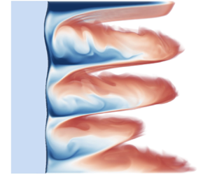
To reveal the effect of salinity on the shape evolution and the melt rate of the ice, we begin with a qualitative description of how the melt front shape depends on the vertical salinity gradient ${\rm \Delta} S_v$. In figure 2(c–e) typical temperature and salinity fields for three different 3D simulations are shown, where we fix ${\rm \Delta} T=20\ {\rm K}$, $H=5\ {\rm cm}$, $S_m=5\ {\rm g} \ {\rm kg}^{-1}$, and vary ${\rm \Delta} S_v$.

Figure 2.

(a) An illustration of the simulation set-up. Initially, the ice block is set at the right sidewall, the temperature of the water is set to be uniform as ${\rm \Delta} T$ and the salinity of the water is set with a vertical gradient depending on $S_m$ and ${\rm \Delta} S_v$. (b) Plot of relative density $\varDelta \rho$ versus temperature for different salinities. The dots mark the melting points. (c–e) Snapshots of temperature (left column), salinity field (centre) and contour of melt front (right) at (c) $S_v=0$, (d) $S_v=5\ {\rm g}\ {\rm kg}^{-1}$ and (e) $S_v=10\ {\rm g}\ {\rm kg}^{-1}$.

At relatively low or zero vertical salinity variation ${\rm \Delta} S_v =0$ (figure 2c), when there is no initial stable stratification, salinity and temperature are mostly uniform in the bulk, and a concave ice melt front forms because of the large-scale circulation, as shown in figure 2(c), right. At moderate ${\rm \Delta} S_v (=5\ {\rm g}\ {\rm kg}^{-1})$ (figure 2d), a layered structure occurs for the temperature and salinity fields, and correspondingly also for the ice melt front, similarly to the experiments of Huppert & Turner (Reference Huppert and Turner1980). With a further increase in ${\rm \Delta} S_v(=10\ {\rm g}\ {\rm kg}^{-1})$ (figure 2e), more layers appear in the liquid phase as compared to the case of ${\rm \Delta} S_v=5\ {\rm g}\ {\rm kg}^{-1}$, while the layer structure disappears on the melt front, since the convective flow at the interface is weakened by the stronger stable stratification. In figure 2(e), the top salinity value approaches zero, causing the fresh meltwater plume to intrude at the base of the broad upper layer. This colder plume, with the same salinity as the layer, enters at a level of neutral buoyancy. By contrast, for figure 2(c,d), the less saline meltwater forms a thin layer at the top of the domain. The density contrast between this thin upper layer and the ambient creates strong local stratification, hindering circulation and heat transport to the upper ice. This results in a concave shape at the top. In figure 2(e), warm water is transported to the upper ice through convection.

With this qualitative behaviour established, we now focus on a more detailed analysis of how both vertical and horizontal variations in salinity affect the system. In figure 3(a), we present the temperature and salinity fields from two-dimensional (2D) simulations at various horizontal and vertical salinity variations $S_m$ and ${\rm \Delta} S_v$. One can see that the structure of the flow and melt front depends mainly on ${\rm \Delta} S_v$. Therefore, the vertical salinity gradient and horizontal temperature gradients are the main driving factors of the flow structure, consistent with the findings of Huppert & Turner (Reference Huppert and Turner1980) and Chong et al. (Reference Chong, Yang, Wang, Verzicco and Lohse2020). Note that Weady et al. (Reference Weady, Tong, Zidovska and Ristroph2022) found a similar layer pattern in ice melting in fresh water near $4\,^\circ$C, which is explained by the density anomaly for fresh water. Unlike in fresh water, the layers in salty water are due to the competition between thermal and salinity-driven buoyancy.

Figure 3.

(a) Instantaneous snapshots of temperature field (left) and salinity field (right) for various $S_m$ and ${\rm \Delta} S_v$. The velocity field is shown by arrows in the temperature field. (b) The layer thickness $h$ per unit density as function of the density gradient, following the same representation as in figure 10 of Huppert & Turner (Reference Huppert and Turner1980). The reference density is $\rho _0$ and $\varDelta \rho _T=\rho (0, S_{\infty })-\rho (T_{\infty }, S_{\infty })$. The dashed line represents the theoretical result ($h$) (3.1).

The different diffusivities of heat and salt play a significant role in the dynamics outside the thin fresh layer. Since heat diffuses much faster than salt ($Le=100$), a region of cold, saline water is produced, which sinks because of thermal-induced buoyancy. At ${\rm \Delta} S_v = 0$, the lack of salt stratification allows this water to sink. The accumulation of cold water causes thicker ice at the bottom than in the middle; see the leftmost column in figure 3(a). Combined with the accumulation of fresh water at the top, which weakens the flow, this results in a concave shape for the ice, with the thinnest ice in the middle.

At ${\rm \Delta} S_v=5\ {\rm g}\ {\rm kg}^{-1}$, the physical explanation of the observed layer formation is as follows: after the ice starts to melt, there is an accumulation of cold water outside the thin fresh boundary layer. Being heavier than the surrounding fluid, the cold water sinks. The surrounding fluid, however, becomes denser with depth as the local salinity also increases, and eventually the cold water reaches a neutral buoyancy level, thus producing a sequence of layers as seen in figure 3(a). In this case, vertically stacked convection rolls form. The layered convection rolls sculpt a layered pattern in the melt front, since these rolls bring warm water from the bulk to the melt front and cause non-uniform heat flux at the interface. At ${\rm \Delta} S_v=10\ {\rm g}\ {\rm kg}^{-1}$, more layers in flow structure appear as compared to the case of ${\rm \Delta} S_v=5\ {\rm g}\ {\rm kg}^{-1}$, in accordance with our physical explanation of neutral buoyancy levels, while the amplitude of the layers becomes smaller than in the case of ${\rm \Delta} S_v=5\ {\rm g}\ {\rm kg}^{-1}$, owing to the weaker flow by the stable stratification. In contrast, at the top, the flow is still stronger because the water is relatively fresh. Thus, the ice morphology is closely linked to flow structures, such as layer formation and convective circulation. The ice morphology regimes depend intrinsically on the flow regimes. Chong et al. (Reference Chong, Yang, Wang, Verzicco and Lohse2020) investigated in more detail the flow structures and regime transitions between the convection-dominated regime and the stratification-dominated regime.

We next quantitatively describe the layer height $h$ of the melt front, which occurs in the presence of a stable stratification. We measure the layer thicknesses by calculating the distances between the maximum points at the contour of the ice front ($\phi =0.5$) and then average all these distances as the layer thicknesses. From the analysis of Huppert & Turner (Reference Huppert and Turner1980), by balancing the horizontal density difference due to temperature and the vertical density gradient due to salinity, one can quantify the thickness of these layers as

(3.1)\begin{equation} h=(0.65 \pm 0.06)[\rho(0, S_{\infty})-\rho(T_{\infty}, S_{\infty})]\left(\frac{\mathrm{d} \rho}{\mathrm{d} z}\right)^{{-}1},\end{equation}

where $\rho (T,S)$ is the fluid density at temperature $T$ and salinity $S$, ${\rm d}\rho /{\rm d}z$ is the ambient density stratification, and the subscript $\infty$ in $T_\infty$ and $S_\infty$ relates to the mean far-field value.

In figure 3(b), we plot the mean layer thickness $h$, normalized by the horizontal density difference, as a function of the stratification. We present data both from our simulations and also from the experiments of Huppert & Turner (Reference Huppert and Turner1980). Our simulation results agree very well quantitatively with the experimental data, with (3.1) also giving a good prediction of the layer thickness $h$. Moreover, our results on the melt front shape match well with those of Huppert & Turner (Reference Huppert and Turner1980), which can also be regarded as validation of our simulations of ice melting in saline water.

4. Physical mechanism of the dependence of the average melt rate on salinity

Our objective now is to quantify how salinity variations affect the average melt rate. In figure 4(a), we plot the volume of ice $V(t)$ (normalized by its initial value $V_0$) as a function of time for different $S_m$ with ${\rm \Delta} S_v=5\ {\rm g}\ {\rm kg}^{-1}$, ${\rm \Delta} T=20\ {\rm K}$ and $H=5\ {\rm cm}$. Interestingly, the melt rate shows a non-monotonic relationship with the mean ambient salinity $S_m$; see figure 4(b). In that figure, to further quantify the melt rate, we have calculated the average melt rate $\bar {f}=1/t_{1/2}$, where $t_{1/2}$ represents the time needed to melt half of the initial volume, shown as a dashed line in figure 4(a), and we show $\bar {f}$ as a function of $S_m$ for various ${\rm \Delta} S_v$. We normalize these results relative to the melt rate observed in the absence of salinity. From the data points, one can see a non-monotonic dependence of $\bar {f}$ on $S_m$ in both 2D and 3D simulations: as $S_m$ increases, $\bar {f}$ first decreases and then increases, with a local minimum point depending on ${\rm \Delta} S_v$. Note that we also tried using different thresholds to calculate $\bar {f}$; these change the absolute value of $\bar {f}$, but the trend remains the same. The drivers of this non-monotonicity are not obvious, motivating us to analyse what causes a minimum in the melt rate.

Figure 4.

(a) The normalized volume of ice $V(t)/V_0$ as a function of time $t/t_f$, where $t_f$ is the free-fall time unit. The dashed line represents the location of half of the initial ice volume. (b) The normalized melt rate $\bar {f}/\bar {f}_0$ as a function of $S_m$ for various ${\rm \Delta} S_v$ (colour-coded), where $\bar {f}_0$ is the melt rate without salinity. Circle data points represent 2D simulations, and square data points represent 3D simulations. The red circle data points represent the location of the minimum $\bar {f}$.

To understand this behaviour, we consider the force (per unit mass) balance in the system. A similar argument was adopted for melting in fresh water (Yang et al. Reference Yang, Chong, Liu, Verzicco and Lohse2022a), where the density maximum plays an important role. An illustration of the main sources of dominating terms driving the flow is shown in figure 5(a). The work of raising/sinking the fluid parcel in the stable stratification (${\rm \Delta} S_v$) is done by the buoyancy force, which is driven by both temperature ${\rm \Delta} T$ and salinity $S_m$. When $S_m$ is small, the temperature dominates the buoyancy, and the cold fresh meltwater moves downward (since the temperature is much larger than $4\,^\circ$C, so that the density maximum effect can be neglected). A circulation flow forms and transports cold water away from the ice and warm water towards the ice. When $S_m$ is large, the salinity dominates the buoyancy, and the cold fresh meltwater moves upward; a circulation flow is again generated and efficiently melts the ice. However, at intermediate $S_m$, the temperature- and salinity-induced buoyancy compensate for each other. In this case, fresh meltwater has almost the same density as the surroundings, which weakens the buoyancy-driven flow. The weakened flow near the melt front can be seen from figure 5(b), where we plot the vertical velocity profile in the horizontal direction for three different values of $S_m$. The value $S_m = 3.5\ {\rm g}\ {\rm kg}^{-1}$ is the one where the buoyancy due to the salt concentration and the buoyancy due to thermal effects compensate for each other, and where hence we find the lowest melting rate. More details of the velocity fields are shown in figure 6, following the same cases shown in figure 5(b). Frome figure 6(b,c), one can see that the magnitude of the velocity is correlated with the local melt rates: the location with a faster melt rate also has a larger velocity.

Figure 5.

(a) An illustration of the effects of temperature and salinity. The red and blue colours represent the buoyancy force driven by $T$ and $S$, with the arrows showing the direction of buoyancy. The black line represents the stable stratification. (b) The instantaneous vertical velocity profile (in free-fall velocity units) at mid-height along $x$. The quantity $S_m=3.5\ {\rm g}\ {\rm kg}^{-1}$ corresponds to the minimum melt rate. The inset figure illustrates the $T(x)$, $S(x)$ and $\rho (x)$ profiles at different ambient $S_m$. The dashed line shows the location of the melt front. (c) Location of the minimal melt rate in the parameter space spanned by $\varLambda _T$ and $\varLambda _S$ for various ${\rm \Delta} T$ and $H$. The dashed lines show the prediction from (4.1) and $\varLambda _S=1$ for reference. Regime I is ‘$T$-driven buoyancy’, regime II is ‘$S$-driven buoyancy’ and regime III is ‘fresh layer formation’. The shaded area shows the upper and lower bounds of $\varLambda _S$ from the simulation results.

Figure 6.

The instantaneous vertical velocity profiles at different heights along $x$. for ${\rm \Delta} S_v=0$ and (a) $S_m=0$; (b) $S_m=3.5\ {\rm g}\ {\rm kg}^{-1}$; (c) $S_m=10\ {\rm g}\ {\rm kg}^{-1}$, the same cases as in figure 5(b). (d–f) shows the instantaneous vertical velocity profiles at mid-height as a function of time, corresponding to the cases in (a–c). The black lines show the location of the ice front.

Quantitatively, when the stable stratification is weak, we consider the force balance between the thermal-driven buoyancy to raise the fluid parcel $F_{{\rm \Delta} T}=\frac {1}{2}C_bg{\rm \Delta} T^2$, and the saline-driven buoyancy $F_{{S_m}}=b_0gS_m$, both based on the equation of state (2.8) given above. We obtain

(4.1)\begin{equation} \tfrac{1}{2}C_bg{\rm \Delta} T^2=b_0gS_m\quad {\rm or}\quad \varLambda_T=1,\end{equation}

which means that the temperature- and salinity-induced buoyancies compensate for each other.

To check whether the results agree with the theory, we calculate the values of $\varLambda _T$ and $\varLambda _S$ corresponding to all minimum melt rate points. Then, in figure 5(c), we plot them in the parameter space spanned by $\varLambda _T$ and $\varLambda _S$ for various ${\rm \Delta} T$ and $H$. It can be seen that the data points for different ${\rm \Delta} T$ and $H$ follow the same trend of $\varLambda _T=1$ (I–II) at low ${\rm \Delta} S_v$. We also notice that at high ${\rm \Delta} S_v$, the minimum melt rate points instead follow roughly $\varLambda _S\sim 1$ (II–III) and are independent of the $\varLambda _T$, with a transition between the different regimes. We give our explanation on this second regime (II–III): when the stable stratification is strong (e.g. for large ${\rm \Delta} S_v$, rightmost column of figure 3a), at low $S_m$ a layer of fresh water emerges at the top, which has melted away faster because of the reduced local stratification. At large $S_m$, the salinity-induced buoyancy becomes larger, also resulting in stronger convection and thus faster melting. Therefore, the melt rate has a minimum at medium $S_m$, which results from the competition between buoyancy-driving and local stratification, which is modified by the fresh layer formation at low $S_m$.