





1. Introduction
In recent years, the dynamics of the flow field and aerodynamic loading on rotating wings at low Reynolds numbers have attracted significant scientific interest. This interest arises from the similarity between these conditions and the rotational phase of insect-wing motion. This analogy has motivated extensive study of leading-edge vortex (LEV) stability mechanisms on rotating wings. Researchers have proposed numerous unsteady mechanisms to explain the increased lift of insect wings (Dickinson, Lehmann & Sane Reference Dickinson, Lehmann and Sane1999; Sane Reference Sane2003; Sun Reference Sun2014; Chin & Lentink Reference Chin and Lentink2016). A key mechanism is the formation and stable attachment of the LEV, which enhances lift on insect wings (Ellington et al. Reference Ellington, Van Den, Coen, Alexander and Thomas1996; Van Den Berg & Ellington Reference Van Den and Ellington1997; Birch & Dickinson Reference Birch and Dickinson2001; Srygley & Thomas Reference Srygley and Thomas2002; Usherwood & Ellington Reference Usherwood and Ellington2002; Sane Reference Sane2003; Mao & Jianghao Reference Mao and Jianghao2004). Previous studies have proposed theories to explain LEV stability over rotating wings, such as spanwise vorticity convection from the LEV to the wing tip (Ellington et al. Reference Ellington, Van Den, Coen, Alexander and Thomas1996; Usherwood & Ellington Reference Usherwood and Ellington2002; Birch, Dickson & Dickinson Reference Birch, Dickson and Dickinson2004; Mao & Jianghao Reference Mao and Jianghao2004) and downwash induced by tip vortices (Birch & Dickinson Reference Birch and Dickinson2001), and by the spanwise gradient of incident velocity (Chen, Wu & Zhang Reference Chen, Wu and Zhang2025). Lentink & Dickinson (Reference Lentink and Dickinson2009a , Reference Lentink and Dickinsonb ) highlighted the significance of rotational accelerations (centrifugal, Coriolis, Euler) in maintaining LEV stability and thereby augmenting lift. Similar findings on the role of rotational accelerations have been noted by Jardin & David (Reference Jardin and David2014, Reference Jardin and David2015) and Paulson, Jardin & Buchholz (Reference Paulson, Jardin and Buchholz2023). Among the rotational accelerations, centrifugal acceleration (a radial acceleration that causes the fluid to follow a curved path) and Coriolis acceleration (arising from the relative velocity between the fluid and the rotating frame) critically affect the LEV dynamics during the quasi-steady phase (steady rotation). In contrast, Euler acceleration (associated with angular acceleration of the rotating frame) is pivotal during the transient wing motion phase (acceleration/deceleration). Numerous studies have examined the influence of these rotational accelerations on the flow dynamics and lift evolution, as detailed in the following sections.
1.1. Effects of Euler acceleration
Euler acceleration governs the transient phase of wing motion, where angular velocity is changing. A consistent finding across multiple studies is that wing acceleration enhances transient lift growth. Pitt Ford & Babinsky (Reference Ford and Babinsky2011), Jones & Babinsky (Reference Jones and Babinsky2010); Chen, Wu & Cheng (Reference Chen, Wu and Cheng2020); Mancini et al. (Reference Mancini, Manar, Granlund, Ol and Jones2015); Van Veen et al. (Reference van Veen, van Leeuwen, van Oudheusden and Muijres2022); Chowdhury & Ringuette (Reference Chowdhury and Ringuette2019) and Gururaj et al. (Reference Gururaj, Morris, Moaven, Thurow and Raghav2025) reported that lift growth increases with acceleration during this phase, achieving a higher peak lift. Similar observations have been made for the drag force on an accelerating $90^\circ$
flat plate (Grift et al. Reference Grift, Vijayaragavan, Tummers and Westerweel2019; Fernando, Weymouth & Rival Reference Fernando, Weymouth and Rival2020; Li et al. Reference Li, Xiang, Qin, Liu and Wang2022; Reijtenbagh, Tummers & Westerweel Reference Reijtenbagh, Tummers and Westerweel2023). Several studies, including Mancini et al. (Reference Mancini, Manar, Granlund, Ol and Jones2015), Chen et al. (Reference Chen, Wu and Cheng2020), Reijtenbagh et al. (Reference Reijtenbagh, Tummers and Westerweel2023) and Gururaj et al. (Reference Gururaj, Morris, Moaven, Thurow and Raghav2025), also analysed the impact of wing acceleration on the flow field, noting faster vortex growth and increased instantaneous circulation with higher acceleration. However, Chen et al. (Reference Chen, Wu and Cheng2020) found that acceleration beyond a threshold did not further influence vortex growth. To understand the mechanisms of vorticity amplification, Chen, Wu & Cheng (Reference Chen, Wu and Cheng2019) applied the vorticity-transport equation and identified tangential vorticity convection as the key contributor to LEV transport during the acceleration phase. These studies collectively establish that Euler acceleration directly modifies LEV growth and circulation, thereby governing the intensity of transient lift.
$90^\circ$
flat plate (Grift et al. Reference Grift, Vijayaragavan, Tummers and Westerweel2019; Fernando, Weymouth & Rival Reference Fernando, Weymouth and Rival2020; Li et al. Reference Li, Xiang, Qin, Liu and Wang2022; Reijtenbagh, Tummers & Westerweel Reference Reijtenbagh, Tummers and Westerweel2023). Several studies, including Mancini et al. (Reference Mancini, Manar, Granlund, Ol and Jones2015), Chen et al. (Reference Chen, Wu and Cheng2020), Reijtenbagh et al. (Reference Reijtenbagh, Tummers and Westerweel2023) and Gururaj et al. (Reference Gururaj, Morris, Moaven, Thurow and Raghav2025), also analysed the impact of wing acceleration on the flow field, noting faster vortex growth and increased instantaneous circulation with higher acceleration. However, Chen et al. (Reference Chen, Wu and Cheng2020) found that acceleration beyond a threshold did not further influence vortex growth. To understand the mechanisms of vorticity amplification, Chen, Wu & Cheng (Reference Chen, Wu and Cheng2019) applied the vorticity-transport equation and identified tangential vorticity convection as the key contributor to LEV transport during the acceleration phase. These studies collectively establish that Euler acceleration directly modifies LEV growth and circulation, thereby governing the intensity of transient lift.
The effect of Euler acceleration is often interpreted in terms of added-mass (non-circulatory) and circulatory forces. Added mass refers to the apparent increase in mass when a body accelerates through a fluid, with the corresponding non-circulatory force representing the fluid inertia. The circulatory force, in contrast, is associated with the evolving flow field and vortex development. Several theories suggest that superposing the potential-flow-derived added-mass lift with the circulatory force accurately predicts the forces on an accelerating wing (Chen, Colonius & Taira Reference Chen, Colonius and Taira2010; Percin & Van Oudheusden Reference Percin and van Oudheusden2015; Chowdhury & Ringuette Reference Chowdhury and Ringuette2019; Corkery, Babinsky & Graham Reference Corkery, Babinsky and Graham2019; Manar & Jones Reference Manar and Jones2019; Chen et al. Reference Chen, Wu and Cheng2020). In contrast, other studies argue that the potential flow framework for added mass is inadequate to fully capture acceleration-related forces (Lee et al. Reference Lee, Lua, Lim and Yeo2016b ; Grift et al. Reference Grift, Vijayaragavan, Tummers and Westerweel2019; Fernando et al. Reference Fernando, Weymouth and Rival2020; Reijtenbagh et al. Reference Reijtenbagh, Tummers and Westerweel2023). This divergence indicates that while added-mass concepts provide useful scaling, they may not encompass all unsteady effects relevant to accelerating wings.
Recent work has expanded these interpretations by incorporating classical unsteady aerodynamic models such as the Wagner effect. The Wagner function (Wagner Reference Wagner1925) describes the time-dependent build-up of circulation following a sudden change in wing motion and has been suggested as a useful framework for modelling acceleration-related forces. Studies such as Van Veen et al. (Reference van Veen, van Leeuwen, van Oudheusden and Muijres2022) and Wang et al. (Reference Wang, Goosen and van Keulen2016) have recommended considering Wagner-type contributions alongside added-mass and circulatory terms to improve predictions of lift during the transient phase. Together, these investigations suggest that Euler acceleration influences transient forces through a combination of added-mass effects, evolving circulation and history-dependent unsteady phenomena. While these studies clarify how acceleration influences transient lift, less attention has been given to how such effects interact with rotational accelerations.
1.2. Effects of Coriolis acceleration
A key debate in the literature concerns whether Coriolis acceleration stabilises or destabilises the LEV. Several studies, including Jardin & David (Reference Jardin and David2015) and Jardin (Reference Jardin2017), demonstrated that Coriolis acceleration is crucial for LEV attachment, while centrifugal effects play a comparatively minor role. Limacher, Morton & Wood (Reference Limacher, Morton and Wood2016) found that the Coriolis force significantly alters the spanwise extent of a stable LEV, tilting it from the leading edge into the wake. Similarly, Wabick et al. (Reference Wabick, Johnson, Berdon, Thurow and Buchholz2023) and Paulson et al. (Reference Paulson, Jardin and Buchholz2023) emphasised the importance of Coriolis effects on LEV stability and attachment, although they noted that Coriolis tilting made only a limited contribution to LEV circulation. In contrast, Garmann, Visbal & Orkwis (Reference Garmann, Visbal and Orkwis2013) and Garmann & Visbal (Reference Garmann and Visbal2014) attributed LEV attachment primarily to centrifugal effects, with Coriolis acceleration acting as a destabilising influence. The studies conducted by Ji et al. (Reference Ji, Jin, Huang, Wang, Ravi, Young, Lai and Tian2024) showed that the rotational acceleration terms affect the far-field acoustics. However, the study also showed that the divergence of the convection term in the Navier–Stokes equation dominates over the effects of centrifugal and Coriolis acceleration terms on the acoustics. These opposing conclusions highlight the sensitivity of LEV stability to how rotational accelerations are parameterised and motivate closer examination of governing non-dimensional groups.
Much of this disagreement stems from differences in Rossby number ( $ \textit{Ro}$
) and aspect ratio (
$ \textit{Ro}$
) and aspect ratio ( $ \textit{AR}$
), which strongly modulate Coriolis effects. Lentink & Dickinson (Reference Lentink and Dickinson2009b
) non-dimensionalised the Navier–Stokes equations in a rotating frame to highlight the significance of these parameters, showing that centrifugal and Coriolis accelerations scale with
$ \textit{AR}$
), which strongly modulate Coriolis effects. Lentink & Dickinson (Reference Lentink and Dickinson2009b
) non-dimensionalised the Navier–Stokes equations in a rotating frame to highlight the significance of these parameters, showing that centrifugal and Coriolis accelerations scale with $ \textit{Ro}$
, while viscous terms are associated with the Reynolds number (
$ \textit{Ro}$
, while viscous terms are associated with the Reynolds number ( $ \textit{Re}$
). The Rossby number, defined as the ratio of inertial to Coriolis acceleration, can be expressed as the radius of gyration divided by the wing chord. This radius depends on the root cutout and wing geometry, and is also related to
$ \textit{Re}$
). The Rossby number, defined as the ratio of inertial to Coriolis acceleration, can be expressed as the radius of gyration divided by the wing chord. This radius depends on the root cutout and wing geometry, and is also related to $ \textit{AR}$
, defined as the span-to-chord ratio. Several studies have explored the role of
$ \textit{AR}$
, defined as the span-to-chord ratio. Several studies have explored the role of $ \textit{AR}$
and
$ \textit{AR}$
and $ \textit{Ro}$
in shaping the LEV dynamics. Lee, Lua & Lim (Reference Lee, Lua and Lim2016a
) varied
$ \textit{Ro}$
in shaping the LEV dynamics. Lee, Lua & Lim (Reference Lee, Lua and Lim2016a
) varied $ \textit{AR}$
–
$ \textit{AR}$
– $ \textit{Ro}$
coupling and found that, at fixed
$ \textit{Ro}$
coupling and found that, at fixed $ \textit{Ro}$
, the mean lift coefficient (
$ \textit{Ro}$
, the mean lift coefficient ( $\overline {C_L}$
) increased with
$\overline {C_L}$
) increased with $ \textit{AR}$
until reaching a threshold, beyond which further increases had no effect. Similar results were reported by Garmann & Visbal (Reference Garmann and Visbal2014), Phillips, Knowles & Bomphrey (Reference Phillips, Knowles and Bomphrey2015) and Jardin & Colonius (Reference Jardin and Colonius2018), with Jardin & Colonius (Reference Jardin and Colonius2018) suggesting that optimal lift occurs at
$ \textit{AR}$
until reaching a threshold, beyond which further increases had no effect. Similar results were reported by Garmann & Visbal (Reference Garmann and Visbal2014), Phillips, Knowles & Bomphrey (Reference Phillips, Knowles and Bomphrey2015) and Jardin & Colonius (Reference Jardin and Colonius2018), with Jardin & Colonius (Reference Jardin and Colonius2018) suggesting that optimal lift occurs at $ \textit{AR}$
between 3 and 4 for impulsively started revolving wings. In contrast, Harbig, Sheridan & Thompson (Reference Harbig, Sheridan and Thompson2013), Carr, DeVoria & Ringuette (Reference Carr, DeVoria and Ringuette2015) and Bhat et al. (Reference Bhat, Zhao, Sheridan, Hourigan and Thompson2019) showed that, while moderate increases in
$ \textit{AR}$
between 3 and 4 for impulsively started revolving wings. In contrast, Harbig, Sheridan & Thompson (Reference Harbig, Sheridan and Thompson2013), Carr, DeVoria & Ringuette (Reference Carr, DeVoria and Ringuette2015) and Bhat et al. (Reference Bhat, Zhao, Sheridan, Hourigan and Thompson2019) showed that, while moderate increases in $ \textit{AR}$
initially increase
$ \textit{AR}$
initially increase $\overline {C_L}$
, excessively large
$\overline {C_L}$
, excessively large $ \textit{AR}$
reduces it. These results indicate that the
$ \textit{AR}$
reduces it. These results indicate that the $ \textit{AR}$
–
$ \textit{AR}$
– $ \textit{Ro}$
relationship sets the spanwise flow environment in which Coriolis effects act, making it difficult to disentangle their independent contributions.
$ \textit{Ro}$
relationship sets the spanwise flow environment in which Coriolis effects act, making it difficult to disentangle their independent contributions.
Recent work has refined this picture by considering local Rossby number and spanwise vorticity-transport mechanisms. Lee et al. (Reference Lee, Lua and Lim2016a
) found that decoupling $ \textit{AR}$
and
$ \textit{AR}$
and $ \textit{Ro}$
revealed that increasing
$ \textit{Ro}$
revealed that increasing $ \textit{Ro}$
at fixed
$ \textit{Ro}$
at fixed $ \textit{AR}$
reduced
$ \textit{AR}$
reduced $\overline {C_L}$
. At low
$\overline {C_L}$
. At low $ \textit{Ro}$
, the LEV was coherent from the wing root to two-thirds span, whereas at higher
$ \textit{Ro}$
, the LEV was coherent from the wing root to two-thirds span, whereas at higher $ \textit{Ro}$
it detached around half-span. Similar observations were reported by Schlueter et al. (Reference Schlueter, Jones, Granlund and Ol2014), Smith et al. (Reference Smith, Rockwell, Sheridan and Thompson2017), Jardin & Colonius (Reference Jardin and Colonius2018) and Bhat et al. (Reference Bhat, Zhao, Sheridan, Hourigan and Thompson2019). Jardin (Reference Jardin2017) observed that strong rotational accelerations promoted robust LEV attachment inboard, while the outboard region was unstable. Extending this work, Jardin & Colonius (Reference Jardin and Colonius2018) concluded that the transition from stable to unstable regions is governed by the local Rossby number and occurs near
$ \textit{Ro}$
it detached around half-span. Similar observations were reported by Schlueter et al. (Reference Schlueter, Jones, Granlund and Ol2014), Smith et al. (Reference Smith, Rockwell, Sheridan and Thompson2017), Jardin & Colonius (Reference Jardin and Colonius2018) and Bhat et al. (Reference Bhat, Zhao, Sheridan, Hourigan and Thompson2019). Jardin (Reference Jardin2017) observed that strong rotational accelerations promoted robust LEV attachment inboard, while the outboard region was unstable. Extending this work, Jardin & Colonius (Reference Jardin and Colonius2018) concluded that the transition from stable to unstable regions is governed by the local Rossby number and occurs near $ \textit{Ro}_{\textit{local}} = 3$
. Thus, lower
$ \textit{Ro}_{\textit{local}} = 3$
. Thus, lower $ \textit{Ro}$
supports LEV attachment through strong spanwise flow in the LEV core and wake, which drains spanwise vorticity, balances vorticity production and stabilises the LEV. Wolfinger & Rockwell (Reference Wolfinger and Rockwell2014, Reference Wolfinger and Rockwell2015) and Smith et al. (Reference Smith, Rockwell, Sheridan and Thompson2017) also reported that increasing
$ \textit{Ro}$
supports LEV attachment through strong spanwise flow in the LEV core and wake, which drains spanwise vorticity, balances vorticity production and stabilises the LEV. Wolfinger & Rockwell (Reference Wolfinger and Rockwell2014, Reference Wolfinger and Rockwell2015) and Smith et al. (Reference Smith, Rockwell, Sheridan and Thompson2017) also reported that increasing $ \textit{Ro}$
weakened LEV coherence, whereas Smith et al. (Reference Smith, Rockwell, Sheridan and Thompson2017) and Bhat et al. (Reference Bhat, Zhao, Sheridan, Hourigan and Thompson2019) noted that higher
$ \textit{Ro}$
weakened LEV coherence, whereas Smith et al. (Reference Smith, Rockwell, Sheridan and Thompson2017) and Bhat et al. (Reference Bhat, Zhao, Sheridan, Hourigan and Thompson2019) noted that higher $ \textit{Ro}$
increased LEV circulation by reducing spanwise vorticity convection due to weaker spanwise velocity. In contrast, Phillips, Knowles & Bomphrey (Reference Phillips, Knowles and Bomphrey2017) found that
$ \textit{Ro}$
increased LEV circulation by reducing spanwise vorticity convection due to weaker spanwise velocity. In contrast, Phillips, Knowles & Bomphrey (Reference Phillips, Knowles and Bomphrey2017) found that $\overline {C_L}$
increased with
$\overline {C_L}$
increased with $ \textit{Ro}$
. Jardin & David (Reference Jardin and David2017) further concluded that increasing
$ \textit{Ro}$
. Jardin & David (Reference Jardin and David2017) further concluded that increasing $ \textit{Ro}$
via root cutout inhibited LEV burst, aiding recovery of the pressure drop despite limited aerodynamic performance benefits. More recently, Wabick et al. (Reference Wabick, Johnson, Berdon, Thurow and Buchholz2023) applied the spanwise vorticity-transport formulation and showed that reducing
$ \textit{Ro}$
via root cutout inhibited LEV burst, aiding recovery of the pressure drop despite limited aerodynamic performance benefits. More recently, Wabick et al. (Reference Wabick, Johnson, Berdon, Thurow and Buchholz2023) applied the spanwise vorticity-transport formulation and showed that reducing $ \textit{Ro}$
stabilised the LEV over a larger wing area, while Chen et al. (Reference Chen, Zhou, Werner, Cheng and Wu2023) reported that higher
$ \textit{Ro}$
stabilised the LEV over a larger wing area, while Chen et al. (Reference Chen, Zhou, Werner, Cheng and Wu2023) reported that higher $ \textit{Ro}$
enlarged unsteady regions due to reduced Coriolis tilting and diminished vorticity tilting and stretching. Together, these studies underscore that Coriolis effects cannot be characterised by a single trend; rather, their influence depends on global
$ \textit{Ro}$
enlarged unsteady regions due to reduced Coriolis tilting and diminished vorticity tilting and stretching. Together, these studies underscore that Coriolis effects cannot be characterised by a single trend; rather, their influence depends on global $ \textit{Ro}$
, local
$ \textit{Ro}$
, local $ \textit{Ro}$
, and the spanwise vorticity dynamics.
$ \textit{Ro}$
, and the spanwise vorticity dynamics.
1.3. Motivation and objectives
In summary, prior studies have predominantly examined either the influence of wing acceleration (Euler acceleration) at fixed Rossby numbers or the effects of Rossby number (Coriolis acceleration) on the LEV dynamics and lift during the quasi-steady phase. While these efforts have advanced our understanding of transient and steady contributions separately, they have not fully addressed how the two interact. Research on Rossby number effects specifically during the transient phase of wing motion remains limited. Some studies suggest that higher Rossby numbers enhance maximum lift coefficients in this phase (Schlueter et al. Reference Schlueter, Jones, Granlund and Ol2014; Jardin & Colonius Reference Jardin and Colonius2018), but these observations provide little insight into the underlying physics of transient lift generation or its coupling with flow evolution around the rotating wing. This gap limits understanding of the relative importance of Euler and Coriolis accelerations under different operating conditions.
The objective of this study is therefore to decouple and evaluate the respective roles of Euler and Coriolis accelerations in governing the transient dynamics over a rotating wing. To achieve this, we independently vary wing acceleration and Rossby number, conducting experiments across a broad parametric space while holding pitch angle, aspect ratio and steady-state Reynolds number constant. The Rossby number is utilised here as the governing parameter for the Coriolis acceleration, following the scaling framework of Lentink and Dickinson (Reference Lentink and Dickinson2009a
,Reference Lentink and Dickinson
b
). While $ \textit{Ro}$
also influences the centripetal acceleration, the Coriolis force is the dominant term responsible for regulating the LEV stability, as noted in several past studies. Thus, variations in
$ \textit{Ro}$
also influences the centripetal acceleration, the Coriolis force is the dominant term responsible for regulating the LEV stability, as noted in several past studies. Thus, variations in $ \textit{Ro}$
are interpreted primarily as a regulation of the Coriolis-driven transport mechanisms. Detailed descriptions of experimental methods, parameters and data analysis techniques are provided in § 2. The individual influences of wing acceleration and Rossby number on the transient dynamics are examined in § 3, and a discussion on the relative importance of the Euler and Coriolis accelerations is provided in § 4. The summary and conclusions subsequently follow in § 5. To our knowledge, this is the first systematic experimental study that independently varies Euler and Coriolis accelerations to isolate their respective contributions to transient rotating-wing aerodynamics.
$ \textit{Ro}$
are interpreted primarily as a regulation of the Coriolis-driven transport mechanisms. Detailed descriptions of experimental methods, parameters and data analysis techniques are provided in § 2. The individual influences of wing acceleration and Rossby number on the transient dynamics are examined in § 3, and a discussion on the relative importance of the Euler and Coriolis accelerations is provided in § 4. The summary and conclusions subsequently follow in § 5. To our knowledge, this is the first systematic experimental study that independently varies Euler and Coriolis accelerations to isolate their respective contributions to transient rotating-wing aerodynamics.
2. Experimental methodology
In this section, the description of the experimental apparatus used to conduct the experiments over the rotating wing is detailed, along with the specifics of the force measurement, flow measurement methodology and parameter space considered. Additionally, the vortex identification and circulation measurement methodology, as well as the spanwise vorticity-transport methodology formulation, are discussed.
2.1. Hydrodynamic hover rotor facility
The experiments were conducted in a hydrodynamic hover rotor facility, depicted in figure 1. The facility consists of a $1.2$
m
$1.2$
m $\times \,1.2$
m
$\times \,1.2$
m $\times \,1.2$
m acrylic tank. Around the tank, a T-slotted frame measuring
$\times \,1.2$
m acrylic tank. Around the tank, a T-slotted frame measuring $2.4$
m
$2.4$
m $\times \,1.7$
m
$\times \,1.7$
m $\times \,0.6$
m was constructed to accommodate the rotational actuation mechanism and imaging system. A NEMA 34 stepper motor was used to drive the rotation shaft through timing pulleys and belts, maintaining a 1 : 6 gear ratio between the motor shaft and the rotation shaft. The azimuthal position of the wing was recorded using a US Digital HB6M rotary encoder with a resolution of
$\times \,0.6$
m was constructed to accommodate the rotational actuation mechanism and imaging system. A NEMA 34 stepper motor was used to drive the rotation shaft through timing pulleys and belts, maintaining a 1 : 6 gear ratio between the motor shaft and the rotation shaft. The azimuthal position of the wing was recorded using a US Digital HB6M rotary encoder with a resolution of $5000$
pulses per revolution, providing an angular resolution of
$5000$
pulses per revolution, providing an angular resolution of $0.072^\circ$
. At the opposite end of the rotation shaft, a mirror holder was installed. This holder served dual purposes: housing a load cell for measuring wing loads and mounting a first surface elliptical mirror measuring
$0.072^\circ$
. At the opposite end of the rotation shaft, a mirror holder was installed. This holder served dual purposes: housing a load cell for measuring wing loads and mounting a first surface elliptical mirror measuring $0.12$
m
$0.12$
m $\times \,0.09$
m with
$\times \,0.09$
m with $1/4$
wave flatness. Positioned at an angle of
$1/4$
wave flatness. Positioned at an angle of $50^\circ$
, the mirror facilitated visualisation of the flow field on the suction side and rotated synchronously with the wing. Further details regarding the load and flow-field measurement methodology will be discussed in §§ 2.2 and 2.3.
$50^\circ$
, the mirror facilitated visualisation of the flow field on the suction side and rotated synchronously with the wing. Further details regarding the load and flow-field measurement methodology will be discussed in §§ 2.2 and 2.3.
We performed the experiments on a rectangular flat plate wing with square edges positioned at a pitch angle of $45^\circ$
. The wing had a span (
$45^\circ$
. The wing had a span ( $b$
) of
$b$
) of $110$
mm and a chord (
$110$
mm and a chord ( $c$
) of
$c$
) of $55$
mm, resulting in an aspect ratio (
$55$
mm, resulting in an aspect ratio ( $ \textit{AR}$
) of
$ \textit{AR}$
) of $2$
. We considered a steady-state Reynolds number (
$2$
. We considered a steady-state Reynolds number ( $ \textit{Re}_g$
) of
$ \textit{Re}_g$
) of $3000$
(additional experiments were also conducted at
$3000$
(additional experiments were also conducted at $ \textit{Re}_g = 1000$
, which are discussed in Appendix A), defined at the radius of gyration (as shown in (2.1)). Here,
$ \textit{Re}_g = 1000$
, which are discussed in Appendix A), defined at the radius of gyration (as shown in (2.1)). Here, $\varOmega$
represents the steady-state angular velocity,
$\varOmega$
represents the steady-state angular velocity, $R_g$
denotes the radius of gyration and
$R_g$
denotes the radius of gyration and $\nu$
is the kinematic viscosity
$\nu$
is the kinematic viscosity
 \begin{align} R_g = \sqrt { \int _{r_{c}}^{b + r_{c}}r^2 c/bc \,\text{d}r} \qquad \qquad Ro_g = \frac {R_g}{c} \qquad \qquad Re_g = \frac {\varOmega R_g c}{\nu } . \end{align}
Summary of the experimental conditions considered for $ \textit{Re}_g = 3000$
.
$ \textit{Re}_g = 3000$
.

Computer-aided design representation of the hydrodynamic hover rotor facility (various sub-assemblies are shown in the insets) (adapted from Gururaj et al. (Reference Gururaj, Moaven, Tan, Thurow and Raghav2021)).

The Rossby number ( $ \textit{Ro}_g$
), defined as the ratio of convective to Coriolis acceleration, was defined at the radius of gyration (
$ \textit{Ro}_g$
), defined as the ratio of convective to Coriolis acceleration, was defined at the radius of gyration ( $R_g$
) according to (2.1). In the study, we varied the Rossby number by adjusting the root cutout (
$R_g$
) according to (2.1). In the study, we varied the Rossby number by adjusting the root cutout ( $r_c$
), thereby altering
$r_c$
), thereby altering $R_g$
. Five different Rossby numbers were examined, as detailed in table 1, and schematically depicted in figure 2. The objective of this study was to isolate the effects of Rossby number from wing acceleration. To achieve this, we considered a range of accelerations for each Rossby number. Instead of varying dimensional acceleration, a non-dimensional acceleration parameter
$R_g$
. Five different Rossby numbers were examined, as detailed in table 1, and schematically depicted in figure 2. The objective of this study was to isolate the effects of Rossby number from wing acceleration. To achieve this, we considered a range of accelerations for each Rossby number. Instead of varying dimensional acceleration, a non-dimensional acceleration parameter $\alpha ^*$
was varied.
$\alpha ^*$
was varied. $\alpha ^*$
represents the ratio of Euler acceleration to convective acceleration, as defined in (2.2)
$\alpha ^*$
represents the ratio of Euler acceleration to convective acceleration, as defined in (2.2)
 \begin{align} \alpha ^* = \frac {\dot {\varOmega } c^2}{\varOmega ^2 R_g^2} , \end{align}
where $\dot {\varOmega }$
denotes the angular acceleration of the wing (derivation of
$\dot {\varOmega }$
denotes the angular acceleration of the wing (derivation of $\alpha ^*$
can be found in Gururaj et al. (Reference Gururaj, Morris, Moaven, Thurow and Raghav2025)). It should be noted that, for the aspect ratio, Rossby number and
$\alpha ^*$
can be found in Gururaj et al. (Reference Gururaj, Morris, Moaven, Thurow and Raghav2025)). It should be noted that, for the aspect ratio, Rossby number and $\alpha ^*$
combination and in the measurement volume considered in the study, no dual LEV structures were observed. We employed a linear velocity profile, where the wing reached a steady-state velocity (dictated by
$\alpha ^*$
combination and in the measurement volume considered in the study, no dual LEV structures were observed. We employed a linear velocity profile, where the wing reached a steady-state velocity (dictated by $ \textit{Re}_g$
) under constant acceleration. Figure 3(a) illustrates an example motion profile for different Rossby numbers and
$ \textit{Re}_g$
) under constant acceleration. Figure 3(a) illustrates an example motion profile for different Rossby numbers and $\alpha ^*$
.
$\alpha ^*$
.
Schematic showing the different Rossby numbers considered in the study along with the root cutouts. The figure is not to scale.

(a) Motion profile considered for the rotating flat plate for $ \textit{Ro}_g = 2$
(red),
$ \textit{Ro}_g = 2$
(red), $ \textit{Ro}_g = 3$
(green) and
$ \textit{Ro}_g = 3$
(green) and $ \textit{Ro}_g = 4.5$
(blue) under different
$ \textit{Ro}_g = 4.5$
(blue) under different $\alpha ^*$
conditions. (b) Temporal variation of raw, averaged and filtered lift force.
$\alpha ^*$
conditions. (b) Temporal variation of raw, averaged and filtered lift force.

2.2. Load measurement
The lift force experienced by the wing was measured using an ATI Nano-17/IP68 six-axis load cell. This load cell has a resolution of $1/320$
N for force and
$1/320$
N for force and $1/64$
N-mm for torque in all three directions. To minimise fluid dynamic interference, the load cell, depicted in the inset of figure 1, was installed inside the mirror holder. The mounting configuration ensured that the
$1/64$
N-mm for torque in all three directions. To minimise fluid dynamic interference, the load cell, depicted in the inset of figure 1, was installed inside the mirror holder. The mounting configuration ensured that the $x$
- and
$x$
- and $y$
-axes of the load cell aligned with the directions of lift and drag forces experienced by the wing, respectively. Data acquisition of loads and encoder data was performed using an NI USB-6341 data acquisition system at a sampling rate of
$y$
-axes of the load cell aligned with the directions of lift and drag forces experienced by the wing, respectively. Data acquisition of loads and encoder data was performed using an NI USB-6341 data acquisition system at a sampling rate of $5000$
Hz. For each operating condition, five runs were acquired and averaged. The averaged data were then filtered using a fourth-order low-pass Butterworth filter with a cutoff frequency equal to the acceleration frequency (acceleration frequency is defined as the inverse of the time taken by the wing to accelerate to the steady state). This cutoff frequency was chosen to capture maximum lift without attenuation across all conditions. The raw, averaged and the filtered force signals are shown in figure 3(b).
$5000$
Hz. For each operating condition, five runs were acquired and averaged. The averaged data were then filtered using a fourth-order low-pass Butterworth filter with a cutoff frequency equal to the acceleration frequency (acceleration frequency is defined as the inverse of the time taken by the wing to accelerate to the steady state). This cutoff frequency was chosen to capture maximum lift without attenuation across all conditions. The raw, averaged and the filtered force signals are shown in figure 3(b).
2.3. Flow-field measurement
The three-dimensional (3-D) and time-resolved flow field around the rotating wing was measured using the rotating 3-D velocimetry (‘R3DV’) methodology (Gururaj et al. Reference Gururaj, Moaven, Tan, Thurow and Raghav2021). This technique employs a rotating mirror at the hub to visualise the flow field in the rotating frame, as illustrated in figure 4. A stationary plenoptic camera, mounted co-axially with the mirror, captures images, while a volumetric light source illuminates the flow field. As the wing rotates, the evolving flow field over the wing is reflected onto the mirror, which is then captured by the co-axially mounted camera. This enables the user to continuously study the 3-D, time-resolved flow field over the rotating wing.
Schematic (not to scale) of the rotating 3-D velocimetry methodology (Gururaj et al. Reference Gururaj, Moaven, Tan, Thurow and Raghav2021).

The plenoptic camera utilised in this methodology resembles a conventional camera but includes a microlens array positioned between the main lens and the image sensor. These microlenses split incoming light rays based on their angle of incidence, enabling plenoptic cameras to capture both spatial and angular information of the light striking the sensor (Fahringer, Lynch & Thurow Reference Fahringer, Lynch and Thurow2015). Through computational photography techniques, pixels from a raw plenoptic image can be decoded, allowing for the synthesis of images with varying focal points (‘refocusing’) and viewing angles (‘perspective shifting’). By synthesising multiple perspective views, the parallax of objects and hence their 3-D distances can be determined. These capabilities render the plenoptic camera an effective tool for obtaining instantaneous 3-D measurements of a flow field.
Acquisition rate, dimensions of the measurement volume and the vector grid for each Rossby number condition.

(a) Schematic of the measurement volume considered for R3DV measurements. (b) Three-dimensional flow field measured using R3DV methodology. The 3-D flow field is depicted by the iso-surface of spanwise vorticity and the slice showing the flow field at the radius of gyration.

In this study, the plenoptic imaging system utilised a Nikon $200$
mm main lens and a relay lens, both mounted co-axially on the same optical axis as the mirror, which was connected to a Phantom VEO 4K 990L high-speed camera (further details on the details and architecture of the plenoptic imaging system can be found in the papers by Tan et al. (Reference Tan, Johnson, Clifford and Thurow2019), Alarcon et al. (Reference Alarcon2020) and Tan & Thurow (Reference Tan and Thurow2020)). This camera can capture images at
$200$
mm main lens and a relay lens, both mounted co-axially on the same optical axis as the mirror, which was connected to a Phantom VEO 4K 990L high-speed camera (further details on the details and architecture of the plenoptic imaging system can be found in the papers by Tan et al. (Reference Tan, Johnson, Clifford and Thurow2019), Alarcon et al. (Reference Alarcon2020) and Tan & Thurow (Reference Tan and Thurow2020)). This camera can capture images at $938$
fps with a resolution of
$938$
fps with a resolution of $4096 \times 2304$
pixels. The relay lens contains a
$4096 \times 2304$
pixels. The relay lens contains a $471 \times 362$
array of hexagonal close-packed microlenses, each with a pitch of
$471 \times 362$
array of hexagonal close-packed microlenses, each with a pitch of $0.077$
mm and a focal length of
$0.077$
mm and a focal length of $0.308$
mm. Illumination for the flow field was provided by a LaVision Flashlight–300 LED, emitting warm white light with an intensity peak in the blue spectrum (
$0.308$
mm. Illumination for the flow field was provided by a LaVision Flashlight–300 LED, emitting warm white light with an intensity peak in the blue spectrum ( $445$
nm). Tracer particles used in visualising the flow field were polyamide rhodamine fluorescent particles with diameters ranging from
$445$
nm). Tracer particles used in visualising the flow field were polyamide rhodamine fluorescent particles with diameters ranging from $53{-} 63 \ {\unicode{x03BC}}\rm{m}$
. These particles absorb wavelengths in the range
$53{-} 63 \ {\unicode{x03BC}}\rm{m}$
. These particles absorb wavelengths in the range $430 {-} 565$
nm and emit light in the range
$430 {-} 565$
nm and emit light in the range $590 {-} 625$
nm. A
$590 {-} 625$
nm. A $52$
mm Tiffen Orange 21 filter was inserted into the main lens to filter out reflections from the light source.
$52$
mm Tiffen Orange 21 filter was inserted into the main lens to filter out reflections from the light source.
For data acquisition, we acquired the images in a time-series mode and the acquisition rate for each Rossby number is mentioned in table 2. The measurement volume for capturing the flow field over the rotating wing was centred around the radius of gyration for all Rossby numbers considered, as shown in figure 5. The dimensions of the measurement volume for each cases are tabulated in table 2. The R3DV technique employed a rotating mirror to capture the flow field in the rotating frame of reference, with the camera fixed in the laboratory frame. This arrangement results in a spanwise-rotating field of view within the camera’s frame of reference. To correct for this rotation, a rotational volumetric calibration methodology was used. Detailed information on this calibration and the velocimetry technique can be found in Gururaj et al. (Reference Gururaj, Moaven, Tan, Thurow and Raghav2021).
A plenoptic-adapted particle tracking velocimetry methodology was applied to the calibrated images. Initially, 3-D positions were estimated using light field ray bundling, where particle rays are projected into the measurement volume using image-to-object space mapping. Subsequently, tracking was performed independently within each perspective view to statistically aggregate predicted particle motions over time, aiding in 3-D trajectory estimation. Further details on this plenoptic particle tracking velocimetry methodology in the rotating frame can be found in Moaven et al. (Reference Moaven, Gururaj, Raghav and Thurow2024). The resultant vector grids for each Rossby number case is mentioned in table 2. Furthermore, for all the cases, a vector resolution of $1.25$
mm (
$1.25$
mm ( $0.023c$
) was achieved. Based on the R3DV particle tracking algorithms, the uncertainty in the far-field velocity vectors was estimated to be approximately
$0.023c$
) was achieved. Based on the R3DV particle tracking algorithms, the uncertainty in the far-field velocity vectors was estimated to be approximately $3.6\,\%$
of the steady-state velocity. Here, steady-state velocity is defined as the linear velocity (
$3.6\,\%$
of the steady-state velocity. Here, steady-state velocity is defined as the linear velocity ( $\varOmega r$
) at a distance,
$\varOmega r$
) at a distance, $r$
, from the centre of rotation. It should be noted that a single time-resolved realisation was captured for each kinematic case using R3DV. Unlike conventional methodologies such as 2-D particle image velocimetry (PIV) or tomo-PIV, which often necessitates phase -averaging across multiple cycles to reconstruct the flow history, R3DV provides a continuous, high-resolution volumetric evolution of the flow field throughout the entire wing motion. This allows for the direct calculation of instantaneous quantities – including circulation, growth rates and vorticity-transport quantities – without the errors introduced by phase-averaged independent runs.
$r$
, from the centre of rotation. It should be noted that a single time-resolved realisation was captured for each kinematic case using R3DV. Unlike conventional methodologies such as 2-D particle image velocimetry (PIV) or tomo-PIV, which often necessitates phase -averaging across multiple cycles to reconstruct the flow history, R3DV provides a continuous, high-resolution volumetric evolution of the flow field throughout the entire wing motion. This allows for the direct calculation of instantaneous quantities – including circulation, growth rates and vorticity-transport quantities – without the errors introduced by phase-averaged independent runs.
2.4. Data analysis
In this section, the vortex identification technique used to detect the vortex core is described first. This is followed by a brief description of the spanwise vorticity-transport formulation.
(a) Vortex core detected by the Graftieaux criteria (represented by the black dots). (b) Example control region defined to quantify the terms in the spanwise vorticity-transport equation. The red dotted line represents the line to extract the velocity and vorticity. The flow field is represented by the spanwise vorticity. The black solid line represents the position of the wing.

2.4.1. Vortex identification and circulation estimation
The centre and core of the vortex were estimated using the criteria formulated by Graftieaux, Michard & Grosjean (Reference Graftieaux, Michard and Grosjean2001). Here, the vortex centre is the point at which the fluid is rotating in a vortex, while the vortex core is defined as the region where the flow is rotational. The Graftieaux criteria offers a significant advantage over other vortex identification techniques derived from the velocity gradient tensor due to its robustness against noise in experimental data. The method calculates a scalar field, $\varGamma _1$
, to characterise the location of the centre by considering only the topology of the velocity field and not its magnitude. This scalar function for discrete spatial locations is given by (2.3), where
$\varGamma _1$
, to characterise the location of the centre by considering only the topology of the velocity field and not its magnitude. This scalar function for discrete spatial locations is given by (2.3), where $N$
is the number of points in the grid,
$N$
is the number of points in the grid, $M$
, within a bounded square region centred on the grid point. Here,
$M$
, within a bounded square region centred on the grid point. Here, $\varGamma _1$
is equivalent to the ensemble average of
$\varGamma _1$
is equivalent to the ensemble average of $\sin {\theta _M}$
, where
$\sin {\theta _M}$
, where $\theta _M$
is the angle between the velocity vector (
$\theta _M$
is the angle between the velocity vector ( $U_M$
) and the radius vector (
$U_M$
) and the radius vector ( $R_{\textit{PM}}$
), where
$R_{\textit{PM}}$
), where $P$
is any fixed point in the measurement domain as shown in (2.3). The parameter
$P$
is any fixed point in the measurement domain as shown in (2.3). The parameter $|\varGamma _1|$
is bounded by 1 and is calculated in a 2-D velocity plane in the chordwise direction, where
$|\varGamma _1|$
is bounded by 1 and is calculated in a 2-D velocity plane in the chordwise direction, where $z$
is the unit normal vector of the plane. The centre of the vortex is identified as a local maximum of the
$z$
is the unit normal vector of the plane. The centre of the vortex is identified as a local maximum of the $|\varGamma _1|$
field. Subsequently,
$|\varGamma _1|$
field. Subsequently, $\varGamma _1$
is modified to account for the local advection velocity
$\varGamma _1$
is modified to account for the local advection velocity $U_{\kern-1pt P}$
around
$U_{\kern-1pt P}$
around $P$
to calculate
$P$
to calculate $\varGamma _2$
(2.4). The parameter
$\varGamma _2$
(2.4). The parameter $\varGamma _2$
represents the ratio of the rotation rate (
$\varGamma _2$
represents the ratio of the rotation rate ( $\varOmega _r$
) to the strain rate (
$\varOmega _r$
) to the strain rate ( $\mu$
). Graftieaux et al. (Reference Graftieaux, Michard and Grosjean2001) suggested the regions where
$\mu$
). Graftieaux et al. (Reference Graftieaux, Michard and Grosjean2001) suggested the regions where $|\varGamma _2| \gt 2/\pi$
, are locally dominated by rotation and represent a vortex core (
$|\varGamma _2| \gt 2/\pi$
, are locally dominated by rotation and represent a vortex core ( $\varOmega _{r}/\mu \gt 1$
). The vortex core detected using the Graftieaux criterion is shown in figure 6(a). In the current study, a threshold of
$\varOmega _{r}/\mu \gt 1$
). The vortex core detected using the Graftieaux criterion is shown in figure 6(a). In the current study, a threshold of $\varGamma _1 = 0.6$
and a neighbourhood of
$\varGamma _1 = 0.6$
and a neighbourhood of $5 \times 5$
grid points were selected to identify the vortex centres. These parameters were applied consistently across all cases to ensure a robust detection of the LEV from its initial formation through to the separation stage. Sensitivity testing indicated that lowering the threshold below
$5 \times 5$
grid points were selected to identify the vortex centres. These parameters were applied consistently across all cases to ensure a robust detection of the LEV from its initial formation through to the separation stage. Sensitivity testing indicated that lowering the threshold below $0.6$
led to the detection of experimental noise as spurious vortical structures, whereas substantially increasing the threshold prevented the identification of the LEV during its early stages of development when the vortex is less intense
$0.6$
led to the detection of experimental noise as spurious vortical structures, whereas substantially increasing the threshold prevented the identification of the LEV during its early stages of development when the vortex is less intense
 \begin{align} \varGamma _{1}(P) = \frac {1}{N} \sum _{M} \frac {(\boldsymbol{R}_{\textit{PM}} \wedge \boldsymbol{U}_{\!M}).\boldsymbol{z}}{||\boldsymbol{R}_{\textit{PM}}||.||\boldsymbol{U}_{\!M}||} = \frac {1}{N}\sum _S \sin {\theta _M} , \\[-28pt] \nonumber \end{align}
 \begin{align} \varGamma _{2}(P) = \frac {1}{N} \sum _{M} \frac {[\boldsymbol{R}_{\textit{PM}} \wedge (\boldsymbol{U}_{\!M} - \boldsymbol{U}_{\!P})].\boldsymbol{z}}{||\boldsymbol{R}_{\textit{PM}}||.||\boldsymbol{U}_{\!M} - \boldsymbol{U}_{\!P}||} . \\[0pt] \nonumber \end{align}
With the vortex centre and core identified, the circulation was quantified by integrating the spanwise vorticity in the vortex core as shown in (2.5). In the equation, $\varGamma$
is the circulation,
$\varGamma$
is the circulation, $\omega$
is the vorticity and
$\omega$
is the vorticity and $A$
is the area of the vortex core detected by the criterion, with
$A$
is the area of the vortex core detected by the criterion, with $\omega$
being calculated by taking the curl of the velocity field. As dual LEV structures were not observed within the current parametric space, the circulation determined using the Graftieaux criteria corresponds exclusively to the evolution of a single primary LEV
$\omega$
being calculated by taking the curl of the velocity field. As dual LEV structures were not observed within the current parametric space, the circulation determined using the Graftieaux criteria corresponds exclusively to the evolution of a single primary LEV
 \begin{align} \varGamma = \int _{A} \omega\,\text{d}A . \end{align}
In addition to the calculation of the primary vorticity, the secondary vorticity was also isolated using a modified application of the Graftieaux criterion. While $\varGamma _2 \gt 2/\pi$
was used for the LEV, regions of secondary vorticity were delineated by selecting areas where
$\varGamma _2 \gt 2/\pi$
was used for the LEV, regions of secondary vorticity were delineated by selecting areas where $\varGamma _2 \lt 0$
. This topological thresholding allows for an objective identification of organised counter-rotational structures, independent of local vorticity magnitude. The circulation of the secondary vorticity was then determined by integrating the spanwise vorticity within these identified boundaries. This method was applied consistently across all cases to ensure the reproducibility of the growth rate calculations, even in cases where the secondary vorticity was closely adhered to the wing surface.
$\varGamma _2 \lt 0$
. This topological thresholding allows for an objective identification of organised counter-rotational structures, independent of local vorticity magnitude. The circulation of the secondary vorticity was then determined by integrating the spanwise vorticity within these identified boundaries. This method was applied consistently across all cases to ensure the reproducibility of the growth rate calculations, even in cases where the secondary vorticity was closely adhered to the wing surface.
2.4.2. Transport of spanwise vorticity
In this study, the spanwise vorticity-transport formulation developed by Buchholz et al. (Reference Buchholz, Thurow, Wabick, Johnson, Berdon and Randal2019) and Wabick et al. (Reference Wabick, Johnson, Berdon, Thurow and Buchholz2023) was employed to analyse the mechanisms influencing the growth of the LEV under varying operating conditions. The analysis was conducted within a rotating frame of reference (non-inertial frame) attached to the wing, within a rectangular planar control region (an example is depicted in figure 6(b)). The dimensions of the control region varied based on the Rossby number: for $ \textit{Ro}_g = 2$
, it spanned
$ \textit{Ro}_g = 2$
, it spanned $0.013 \leqslant x/c \leqslant 0.239$
and
$0.013 \leqslant x/c \leqslant 0.239$
and $0.019 \leqslant y/c \leqslant 0.247$
; for
$0.019 \leqslant y/c \leqslant 0.247$
; for $ \textit{Ro}_g = 3$
, it covered
$ \textit{Ro}_g = 3$
, it covered $0.011 \leqslant x/c \leqslant 0.238$
and
$0.011 \leqslant x/c \leqslant 0.238$
and $0.021 \leqslant y/c \leqslant 0.248$
; and for
$0.021 \leqslant y/c \leqslant 0.248$
; and for $ \textit{Ro}_g = 4.5$
, it encompassed
$ \textit{Ro}_g = 4.5$
, it encompassed $0.011 \leqslant x/c \leqslant 0.238$
and
$0.011 \leqslant x/c \leqslant 0.238$
and $0.006 \leqslant y/c \leqslant 0.233$
in the
$0.006 \leqslant y/c \leqslant 0.233$
in the $x$
and
$x$
and $y$
directions, respectively. The analysis was conducted at multiple spanwise locations. The control region used for calculating the terms in the vorticity-transport equation was sized based on the maximum spatial extent of the LEV observed across the entire parametric space. Most of the quantitative analysis was restricted to the transient phase of the wing motion, during which the LEV remains in close proximity to the wing. Furthermore, during the transient phase, only the primary LEV is formed. Therefore, the control region is not contaminated by other vortical structures, and only the effects of the primary LEV and the secondary vorticity are captured in it. To ensure the robustness of the integration, the region dimensions were determined using the most protracted LEV development case (
$y$
directions, respectively. The analysis was conducted at multiple spanwise locations. The control region used for calculating the terms in the vorticity-transport equation was sized based on the maximum spatial extent of the LEV observed across the entire parametric space. Most of the quantitative analysis was restricted to the transient phase of the wing motion, during which the LEV remains in close proximity to the wing. Furthermore, during the transient phase, only the primary LEV is formed. Therefore, the control region is not contaminated by other vortical structures, and only the effects of the primary LEV and the secondary vorticity are captured in it. To ensure the robustness of the integration, the region dimensions were determined using the most protracted LEV development case ( $ \textit{Ro} = 2$
,
$ \textit{Ro} = 2$
, $\alpha ^* = 0.19$
) at the end of its acceleration period, and it was noted that the LEV remained fully inside the defined domain. This ensured that the integration encompasses the entire vortical structure – even during stages of liftoff – and prevents bias in the vorticity-transport metrics or contamination from neighbouring flow structures.
$\alpha ^* = 0.19$
) at the end of its acceleration period, and it was noted that the LEV remained fully inside the defined domain. This ensured that the integration encompasses the entire vortical structure – even during stages of liftoff – and prevents bias in the vorticity-transport metrics or contamination from neighbouring flow structures.
The planar control region’s position and size were strategically chosen to encompass the LEV from its onset through its growth stage. This region, fixed to the wing, enabled the growth of the LEV and secondary vorticity to be captured. Given that the LEV and secondary vorticity are primarily associated with spanwise vorticity, the analysis focused solely on the transport of spanwise vorticity, which is nominally perpendicular to the local direction of travel of the wing. Following Wabick et al. (Reference Wabick, Johnson, Berdon, Thurow and Buchholz2023), the vorticity-transport budget within the planar control region can be expressed as
 \begin{align} \frac {\text{d}\varGamma _z}{\text{d}t} & = -\int _{A} u_z \frac {\partial {\omega _z}}{\partial {z}} \text{d}A - \oint _{\delta A} (u \boldsymbol{\cdot }n_{\delta A})\omega _z\,\text{d}s - \nu \int _{\textit{bound.}\,4} \frac {\partial \omega _z}{\partial y} \text{d}x \nonumber \\& \quad + \int _{A} \left(\omega _x \frac {\partial u_z}{\partial x} + \omega _y \frac {\partial u_z}{\partial y}\right) \text{d}A + \int _{A} \left(2\varOmega _x \frac {\partial u_z}{\partial x} + 2\varOmega _y \frac {\partial u_z}{\partial y}\right) \text{d}A . \end{align}
In (2.6), the left side represents the growth or decay of the circulation in the control region. The terms on the right side represent the spanwise convective flux of vorticity through the planar control region, in-plane convective fluxes of vorticity through the boundaries of the control region, the diffusive flux of vorticity from the wing surface, vorticity tilting and Coriolis tilting. Noting that tilting of a vortex does not change its circulation, Paulson et al. (Reference Paulson, Jardin and Buchholz2023) showed that the spanwise convective flux and tilting flux are not independent, but constituents of an out-of-plane convective flux that constitutes the 3-D component of vorticity transport in the control region. The Coriolis tilting term was considered a correction to the (physical) tilting term, and generally found to have insignificant magnitude. The complete derivation of the vorticity-transport equation can be found in Buchholz et al. (Reference Buchholz, Thurow, Wabick, Johnson, Berdon and Randal2019), Wabick et al. (Reference Wabick, Johnson, Berdon, Thurow and Buchholz2023) and Paulson et al. (Reference Paulson, Jardin and Buchholz2023).
Although the non-inertial accelerations present in the reference frame of the control region include Euler, centripetal and Coriolis accelerations, only Coriolis accelerations contribute to transport in the bulk fluid in (2.6). The surface diffusive flux of spanwise vorticity, from the suction surface of the wing, is dominated by the streamwise component of the surface pressure gradient, Euler and centripetal accelerations, as shown by Buchholz et al. (Reference Buchholz, Thurow, Wabick, Johnson, Berdon and Randal2019)
 \begin{align} \begin{aligned} -\nu \frac {\partial \omega _z}{\partial y} = \frac {1}{\rho } \frac {\partial p}{\partial x} - \dot {\varOmega } r + \varOmega ^2 r, \end{aligned} \end{align}
where the terms on the right side of (2.7) are evaluated on the boundary of the control region adjacent to the wing surface. The second and third terms on the right side are contributions from the Euler acceleration and the centripetal acceleration, respectively.
In (2.6), spanwise convection, vorticity tilting, Coriolis correction and the rate of change of circulation are evaluated within the interior of the control region itself. Meanwhile, the in-plane convective flux is quantified along the boundaries of the control region. The surface diffusive flux is determined by assuming equality between the left and right sides of (2.6). Past studies conducted by Eslam Panah et al. (Reference Panah, Azar, James and Buchholz2015) and Wabick et al. (Reference Wabick, Johnson, Berdon, Thurow and Buchholz2023) used estimates of the surface diffusive flux – derived from surface pressure measurements – to validate this assumption. Spatial derivatives and the temporal derivative of circulation are calculated using a second-order central difference scheme, and the circulation is quantified by integrating the spanwise vorticity inside the control region. Numerical integration within the control region and along its boundaries is performed using the trapezoidal rule.
3. Results and discussion
3.1. Effect of non-dimensional Euler acceleration ( $\alpha ^*$
)
$\alpha ^*$
)

3.1.1. Transient lift generation
Figure 7(a) illustrates the lift variation for a wing at different $\alpha ^*$
values when
$\alpha ^*$
values when $ \textit{Ro}_g = 2$
. Lift is plotted against
$ \textit{Ro}_g = 2$
. Lift is plotted against $\lambda$
, the non-dimensional azimuth defined by (3.1), where
$\lambda$
, the non-dimensional azimuth defined by (3.1), where $\psi$
specifies the azimuth in radians
$\psi$
specifies the azimuth in radians
 \begin{align} \begin{aligned} \lambda = \frac {\psi R_g}{c} \end{aligned} . \end{align}
(a) Temporal evolution of lift experienced by the wing under different $\alpha ^*$
conditions at
$\alpha ^*$
conditions at $ \textit{Ro}_g = 2$
. The dashed lines denote the end of the acceleration phase. (b) Variation of the maximum lift coefficient (
$ \textit{Ro}_g = 2$
. The dashed lines denote the end of the acceleration phase. (b) Variation of the maximum lift coefficient ( $C_{L_{\textit{max}}}$
, circular symbols) and non-circulatory lift coefficient (
$C_{L_{\textit{max}}}$
, circular symbols) and non-circulatory lift coefficient ( $C_{L_{\textit{NC}}}$
, solid line) with
$C_{L_{\textit{NC}}}$
, solid line) with $\alpha ^*$
. In (b),
$\alpha ^*$
. In (b), $C_{L_{\textit{max}}}$
,
$C_{L_{\textit{max}}}$
, $C_{L_{\textit{NC}}}$
and
$C_{L_{\textit{NC}}}$
and $\alpha ^*$
are plotted on logarithmic scales.
$\alpha ^*$
are plotted on logarithmic scales.

Initially, as the wing rotates, lift rises to a peak before decreasing to a steady level for all $\alpha ^*$
. A higher
$\alpha ^*$
. A higher $\alpha ^*$
results in a faster increase in transient lift and a greater maximum lift, although the steady-state lift remains constant. This behaviour is consistent with previous studies (Mancini et al. Reference Mancini, Manar, Granlund, Ol and Jones2015; Grift et al. Reference Grift, Vijayaragavan, Tummers and Westerweel2019; Chen et al. Reference Chen, Wu and Cheng2020; Reijtenbagh et al. Reference Reijtenbagh, Tummers and Westerweel2023; Gururaj et al. Reference Gururaj, Morris, Moaven, Thurow and Raghav2025). As mentioned in § 2, additional experiments were also conducted at
$\alpha ^*$
results in a faster increase in transient lift and a greater maximum lift, although the steady-state lift remains constant. This behaviour is consistent with previous studies (Mancini et al. Reference Mancini, Manar, Granlund, Ol and Jones2015; Grift et al. Reference Grift, Vijayaragavan, Tummers and Westerweel2019; Chen et al. Reference Chen, Wu and Cheng2020; Reijtenbagh et al. Reference Reijtenbagh, Tummers and Westerweel2023; Gururaj et al. Reference Gururaj, Morris, Moaven, Thurow and Raghav2025). As mentioned in § 2, additional experiments were also conducted at $ \textit{Re}_g = 1000$
, the results for which are discussed in Appendix A. The lift evolution trends reported here at
$ \textit{Re}_g = 1000$
, the results for which are discussed in Appendix A. The lift evolution trends reported here at $ \textit{Re}_g = 3000$
are consistent with those observed at
$ \textit{Re}_g = 3000$
are consistent with those observed at $ \textit{Re}_g = 1000$
(shown in Appendix A).
$ \textit{Re}_g = 1000$
(shown in Appendix A).
Figure 7(b) shows the maximum lift at different $\alpha ^*$
, denoted by
$\alpha ^*$
, denoted by $C_{L_{\textit{max}}}$
(3.2). Maximum lift is non-dimensionalised with steady-state dynamic pressure and wing area because it occurs near the end of acceleration, when the angular velocity is near steady state
$C_{L_{\textit{max}}}$
(3.2). Maximum lift is non-dimensionalised with steady-state dynamic pressure and wing area because it occurs near the end of acceleration, when the angular velocity is near steady state
 \begin{align} \begin{aligned} C_{L_{\textit{max}}} = \frac {2 L_{\textit{max}}}{\rho (\varOmega _{ss} R_g)^2 b c} \end{aligned} . \end{align}
In figure 7(b), $C_{L_{\textit{max}}}$
shows minimal change at low
$C_{L_{\textit{max}}}$
shows minimal change at low $\alpha ^*$
but increases with
$\alpha ^*$
but increases with $\alpha ^*$
at higher values. Gururaj et al. (Reference Gururaj, Morris, Moaven, Thurow and Raghav2025) identified these as quasi-steady and acceleration-dominated regimes, respectively. Similar
$\alpha ^*$
at higher values. Gururaj et al. (Reference Gururaj, Morris, Moaven, Thurow and Raghav2025) identified these as quasi-steady and acceleration-dominated regimes, respectively. Similar $C_{L_{\textit{max}}}$
behaviour with
$C_{L_{\textit{max}}}$
behaviour with $\alpha ^*$
is observed for other Rossby numbers. The figure also presents the non-circulatory lift coefficient,
$\alpha ^*$
is observed for other Rossby numbers. The figure also presents the non-circulatory lift coefficient, $C_{L_{\textit{NC}}}$
, calculated from the first term in (3.3) (Percin & Van Oudheusden Reference Percin and van Oudheusden2015; Chowdhury & Ringuette Reference Chowdhury and Ringuette2019)
$C_{L_{\textit{NC}}}$
, calculated from the first term in (3.3) (Percin & Van Oudheusden Reference Percin and van Oudheusden2015; Chowdhury & Ringuette Reference Chowdhury and Ringuette2019)
 \begin{align} \begin{aligned} C_L = \overbrace {\alpha ^* \frac {\pi }{4 b c}\big (b_t^2 - (b_t - b)^2\big ) \sin {\theta } \cos {\theta }}^{\substack {\textit{Non-circulatory lift coefficient}}} + \overbrace {2\!\left (\frac {\text{d}\varGamma _z^*}{\text{d}t^*} + \varGamma _z^*\right )}^{\substack {\textit{Circulatory lift coefficient}}} \end{aligned} . \end{align}
Here, $b_t$
is the wing-tip distance from the rotation centre and
$b_t$
is the wing-tip distance from the rotation centre and $\theta$
is the wing pitch angle. The non-circulatory part depends on wing geometry, orientation and acceleration (
$\theta$
is the wing pitch angle. The non-circulatory part depends on wing geometry, orientation and acceleration ( $\alpha ^*$
), while the circulatory part depends on the rate of change and instantaneous circulation. The equation shows that the non-circulatory component increases linearly with
$\alpha ^*$
), while the circulatory part depends on the rate of change and instantaneous circulation. The equation shows that the non-circulatory component increases linearly with $\alpha ^*$
, as seen in figure 7(b). Under quasi-steady conditions (lower
$\alpha ^*$
, as seen in figure 7(b). Under quasi-steady conditions (lower $\alpha ^*$
), the non-circulatory contribution to maximum lift is minor, indicating a dominance of the circulatory component. However, when acceleration dominates (higher
$\alpha ^*$
), the non-circulatory contribution to maximum lift is minor, indicating a dominance of the circulatory component. However, when acceleration dominates (higher $\alpha ^*$
), the non-circulatory component significantly affects transient lift. Because circulatory lift depends on the flow-field dynamics, we next examine how
$\alpha ^*$
), the non-circulatory component significantly affects transient lift. Because circulatory lift depends on the flow-field dynamics, we next examine how $\alpha ^*$
influences flow evolution.
$\alpha ^*$
influences flow evolution.
3.1.2. Leading-edge vortex evolution
Figure 8 shows the spatio-temporal evolution of the flow field at various $\alpha ^*$
for
$\alpha ^*$
for $ \textit{Ro}_g = 2$
. Iso-surfaces of spanwise vorticity (
$ \textit{Ro}_g = 2$
. Iso-surfaces of spanwise vorticity ( $\omega _z = 10\ \mathrm{s}^{-1}$
) highlight stages of LEV development, with colours indicating spanwise velocity. The sequences suggest that increasing
$\omega _z = 10\ \mathrm{s}^{-1}$
) highlight stages of LEV development, with colours indicating spanwise velocity. The sequences suggest that increasing $\alpha ^*$
at fixed Rossby number advances LEV development with respect to
$\alpha ^*$
at fixed Rossby number advances LEV development with respect to $\lambda$
without changing its spatial evolution. It is already known that higher acceleration will advance the flow development in time. However, our results show that higher acceleration not only accelerates flow development temporally, but the advancement occurs more quickly with azimuthal position of the wing too (LEV evolutions under different
$\lambda$
without changing its spatial evolution. It is already known that higher acceleration will advance the flow development in time. However, our results show that higher acceleration not only accelerates flow development temporally, but the advancement occurs more quickly with azimuthal position of the wing too (LEV evolutions under different $\alpha ^*$
conditions are shown in Movie 1.mp4 are available at https://doi.org/10.1017/jfm.2026.11600). For example, at
$\alpha ^*$
conditions are shown in Movie 1.mp4 are available at https://doi.org/10.1017/jfm.2026.11600). For example, at $\lambda = 0.25$
and
$\lambda = 0.25$
and $\alpha ^* = 0.19$
, no LEV is present (figure 8
a), while higher
$\alpha ^* = 0.19$
, no LEV is present (figure 8
a), while higher $\alpha ^*$
conditions show a clear LEV (figure 8
d,g, j) at this early displacement. At
$\alpha ^*$
conditions show a clear LEV (figure 8
d,g, j) at this early displacement. At $\lambda = 0.5$
, an LEV starts forming for
$\lambda = 0.5$
, an LEV starts forming for $\alpha ^* = 0.19$
(figure 8
b) but is more developed for
$\alpha ^* = 0.19$
(figure 8
b) but is more developed for $\alpha ^* = 0.29$
and
$\alpha ^* = 0.29$
and $1.1$
(figure 8
e,h). For
$1.1$
(figure 8
e,h). For $\alpha ^* = 4.1$
, an arch-type LEV is observed at
$\alpha ^* = 4.1$
, an arch-type LEV is observed at $\lambda = 0.5$
(figure 8
k). As the wing rotates, a similar arch-type LEV appears by
$\lambda = 0.5$
(figure 8
k). As the wing rotates, a similar arch-type LEV appears by $\lambda = 0.75$
for
$\lambda = 0.75$
for $\alpha ^* = 0.29$
and
$\alpha ^* = 0.29$
and $1.1$
(figure 8
f,i), whereas no such structure is seen for
$1.1$
(figure 8
f,i), whereas no such structure is seen for $\alpha ^* = 0.19$
.
$\alpha ^* = 0.19$
.
Spatio-temporal evolution of the flow field over the rotating wing under $\alpha ^* = 0.19$
(a–c),
$\alpha ^* = 0.19$
(a–c), $\alpha ^* = 0.29$
(d–f),
$\alpha ^* = 0.29$
(d–f), $\alpha ^* = 1.1$
(g–i) and
$\alpha ^* = 1.1$
(g–i) and $\alpha ^* = 4.1$
(j–l) at
$\alpha ^* = 4.1$
(j–l) at $ \textit{Ro}_g = 2$
. Flow structures are represented by isosurfaces of spanwise vorticity (
$ \textit{Ro}_g = 2$
. Flow structures are represented by isosurfaces of spanwise vorticity ( $\omega _z = 10\ \mathrm{s}^{-1}$
) and are coloured by spanwise velocity (
$\omega _z = 10\ \mathrm{s}^{-1}$
) and are coloured by spanwise velocity ( $u_z$
).
$u_z$
).

The figures also show positive spanwise flow near the root, diminishing toward mid-span and negative flow further outboard. Positive velocity at the root is due to strong Coriolis effects, and negative velocity near the tip stems from enhanced tip effects. These aspects are analysed further in the next section.
Temporal evolution of the flow field over the rotating wing for $\alpha ^*= 0.19$
(a–c),
$\alpha ^*= 0.19$
(a–c), $\alpha ^* = 0.29$
(d–f),
$\alpha ^* = 0.29$
(d–f), $\alpha ^* = 1.1$
(g–i) and
$\alpha ^* = 1.1$
(g–i) and $\alpha ^* = 4.1$
(j–l) at
$\alpha ^* = 4.1$
(j–l) at $ \textit{Ro}_g = 2$
. Contours of spanwise vorticity with overlaid velocity vectors at mid-span.
$ \textit{Ro}_g = 2$
. Contours of spanwise vorticity with overlaid velocity vectors at mid-span.

To further investigate the effects of $\alpha ^*$
, a 2-D slice at mid-span near the radius of gyration is analysed (figure 9). At
$\alpha ^*$
, a 2-D slice at mid-span near the radius of gyration is analysed (figure 9). At $\lambda = 0.25$
and 0.5, increasing
$\lambda = 0.25$
and 0.5, increasing $\alpha ^*$
strengthens the LEV. For each
$\alpha ^*$
strengthens the LEV. For each $\alpha ^*$
, the LEV strengthens with increasing
$\alpha ^*$
, the LEV strengthens with increasing $\lambda$
as vorticity is continuously fed from the shear layer. By
$\lambda$
as vorticity is continuously fed from the shear layer. By $\lambda = 0.75$
, the LEV detaches from the shear layer for
$\lambda = 0.75$
, the LEV detaches from the shear layer for $\alpha ^* = 1.1$
and
$\alpha ^* = 1.1$
and $4.1$
(figure 9
i,l), while remaining attached for lower
$4.1$
(figure 9
i,l), while remaining attached for lower $\alpha ^*$
(figure 9
c, f). This leads to subsequent weakening of the LEV, which has progressed further for
$\alpha ^*$
(figure 9
c, f). This leads to subsequent weakening of the LEV, which has progressed further for $\alpha ^* = 4.1$
at
$\alpha ^* = 4.1$
at $\lambda = 0.75$
.
$\lambda = 0.75$
.
(a) Temporal evolution of LEV circulation at mid-span under different $\alpha ^*$
conditions at
$\alpha ^*$
conditions at $ \textit{Ro}_g = 2$
. (b) Spanwise variation of the non-dimensional rate of change of circulation at the occurrence of maximum lift,
$ \textit{Ro}_g = 2$
. (b) Spanwise variation of the non-dimensional rate of change of circulation at the occurrence of maximum lift, ${\text{d}\varGamma _{z,max }^*}/{\text{d}t^*}$
, under different
${\text{d}\varGamma _{z,max }^*}/{\text{d}t^*}$
, under different $\alpha ^*$
at
$\alpha ^*$
at $ \textit{Ro}_g = 2$
.
$ \textit{Ro}_g = 2$
.

Figure 10(a) shows LEV circulation ( $\varGamma _z$
) vs
$\varGamma _z$
) vs $\lambda$
at mid-span for different
$\lambda$
at mid-span for different $\alpha ^*$
at
$\alpha ^*$
at $ \textit{Ro}_g = 2$
. Circulation is computed by integrating spanwise vorticity within the LEV core, detected via the Graftieaux criterion (see § 2.4.1). Consistent with figure 9, higher
$ \textit{Ro}_g = 2$
. Circulation is computed by integrating spanwise vorticity within the LEV core, detected via the Graftieaux criterion (see § 2.4.1). Consistent with figure 9, higher $\alpha ^*$
yields faster circulation growth and higher instantaneous circulation, in line with prior work (Mancini et al. Reference Mancini, Manar, Granlund, Ol and Jones2015; Chen et al. Reference Chen, Wu and Cheng2020; Reijtenbagh et al. Reference Reijtenbagh, Tummers and Westerweel2023; Gururaj et al. Reference Gururaj, Morris, Moaven, Thurow and Raghav2025).
$\alpha ^*$
yields faster circulation growth and higher instantaneous circulation, in line with prior work (Mancini et al. Reference Mancini, Manar, Granlund, Ol and Jones2015; Chen et al. Reference Chen, Wu and Cheng2020; Reijtenbagh et al. Reference Reijtenbagh, Tummers and Westerweel2023; Gururaj et al. Reference Gururaj, Morris, Moaven, Thurow and Raghav2025).
Because the LEV is strongly three-dimensional, we examine growth at multiple spanwise locations. Figure 10(b) presents the spatial variation of the maximum LEV growth rate, ${\text{d}\varGamma _{z,max }^*}/{\text{d}t^*}$
, averaged from start of motion to peak lift and non-dimensionalised per (3.4)
${\text{d}\varGamma _{z,max }^*}/{\text{d}t^*}$
, averaged from start of motion to peak lift and non-dimensionalised per (3.4)
 \begin{align} \begin{aligned} \frac {\text{d}\varGamma _{z,max }^*}{\text{d}t^*} = \frac {1}{\varOmega ^2 R_g^2} \frac {\text{d}\varGamma _{z,max }}{\text{d}t} \end{aligned} . \end{align}
Increasing $\alpha ^*$
increases LEV growth rate across the span. For both
$\alpha ^*$
increases LEV growth rate across the span. For both $\alpha ^*$
cases, the growth rate rises from the root toward mid-span, becomes relatively uniform and then decreases toward the tip. This agrees with Jardin (Reference Jardin2017) and Wabick et al. (Reference Wabick, Johnson, Berdon, Thurow and Buchholz2023), who identified a quasi-2-D region near mid-span. Reduced inboard growth is due to lower wing velocity (dynamic pressure) and substantial 3-D effects (Jardin Reference Jardin2017; Wabick et al. Reference Wabick, Johnson, Berdon, Thurow and Buchholz2023), whereas reduced outboard growth is attributed to tip effects. We next consider the transport mechanisms governing LEV growth during the transient phase.
$\alpha ^*$
cases, the growth rate rises from the root toward mid-span, becomes relatively uniform and then decreases toward the tip. This agrees with Jardin (Reference Jardin2017) and Wabick et al. (Reference Wabick, Johnson, Berdon, Thurow and Buchholz2023), who identified a quasi-2-D region near mid-span. Reduced inboard growth is due to lower wing velocity (dynamic pressure) and substantial 3-D effects (Jardin Reference Jardin2017; Wabick et al. Reference Wabick, Johnson, Berdon, Thurow and Buchholz2023), whereas reduced outboard growth is attributed to tip effects. We next consider the transport mechanisms governing LEV growth during the transient phase.
3.1.3. Mechanisms contributing to LEV growth
The spanwise vorticity-transport equation described in § 2.4.2 is used to analyse the mechanisms responsible for LEV growth under various operating conditions. The terms on the left- and right-hand sides of (2.6) are plotted in figure 11 for $\alpha ^* = 0.19$
and
$\alpha ^* = 0.19$
and $ \textit{Ro}_g = 2$
at
$ \textit{Ro}_g = 2$
at $z/b = 0.49$
. Note that the entire
$z/b = 0.49$
. Note that the entire $\lambda$
range in figure 11 lies within the acceleration period. In the figure (and those that follow),
$\lambda$
range in figure 11 lies within the acceleration period. In the figure (and those that follow), ${\text{d}\varGamma _z^*}/{\text{d}t^*}$
is the rate of change of circulation in the control region,
${\text{d}\varGamma _z^*}/{\text{d}t^*}$
is the rate of change of circulation in the control region, $ \textit{IPCF}^{\,*}$
denotes the in-plane convective flux,
$ \textit{IPCF}^{\,*}$
denotes the in-plane convective flux, $ \textit{CCF}^{\,*}$
the Coriolis correction and
$ \textit{CCF}^{\,*}$
the Coriolis correction and $ \textit{SDF}^{\,*}$
the surface diffusive flux. We also plot
$ \textit{SDF}^{\,*}$
the surface diffusive flux. We also plot $ \textit{OPCF}^{\,*}$
(out-of-plane circulation flux), defined as the net out-of-plane vorticity transport due to the combined effects of
$ \textit{OPCF}^{\,*}$
(out-of-plane circulation flux), defined as the net out-of-plane vorticity transport due to the combined effects of $ \textit{SPCF}^{\,*}$
(spanwise convective flux) and
$ \textit{SPCF}^{\,*}$
(spanwise convective flux) and $ \textit{VTF}^{\,*}$
(vorticity tilting flux). The derivation of
$ \textit{VTF}^{\,*}$
(vorticity tilting flux). The derivation of $ \textit{OPCF}^{\,*}$
is provided by Paulson et al. (Reference Paulson, Jardin and Buchholz2023). Fluxes are non-dimensionalised according to the reference values in (3.4).
$ \textit{OPCF}^{\,*}$
is provided by Paulson et al. (Reference Paulson, Jardin and Buchholz2023). Fluxes are non-dimensionalised according to the reference values in (3.4).
Temporal evolution of the terms in the spanwise vorticity-transport equation under $\alpha ^* = 0.19$
and
$\alpha ^* = 0.19$
and $ \textit{Ro}_g = 2$
at
$ \textit{Ro}_g = 2$
at $z/b = 0.49$
.
$z/b = 0.49$
.

The leading-edge shear layer is the primary source of LEV circulation within the control region at $z/b = 0.49$
; during the initial stages of wing motion,
$z/b = 0.49$
; during the initial stages of wing motion, $\text{d}\varGamma _z^*/\text{d}t^*$
is approximately equal to
$\text{d}\varGamma _z^*/\text{d}t^*$
is approximately equal to $ \textit{IPCF}^{\,*}$
. Compared with
$ \textit{IPCF}^{\,*}$
. Compared with $ \textit{IPCF}^{\,*}$
,
$ \textit{IPCF}^{\,*}$
, $ \textit{OPCF}^{\,*}$
remains relatively small. Paulson et al. (Reference Paulson, Jardin and Buchholz2023) noted that
$ \textit{OPCF}^{\,*}$
remains relatively small. Paulson et al. (Reference Paulson, Jardin and Buchholz2023) noted that $ \textit{SPCF}^{\,*}$
and
$ \textit{SPCF}^{\,*}$
and $ \textit{VTF}^{\,*}$
are negatively correlated, and as such, their combined influence, i.e.
$ \textit{VTF}^{\,*}$
are negatively correlated, and as such, their combined influence, i.e. $ \textit{OPCF}^{\,*}$
, on the LEV dynamics is relatively small. Vorticity in both the shear layer and LEV is predominantly positive (figures 9, 10). The diffusive flux, which primarily governs secondary-vorticity generation, is of similar magnitude to the 3-D fluxes, and small in comparison with
$ \textit{OPCF}^{\,*}$
, on the LEV dynamics is relatively small. Vorticity in both the shear layer and LEV is predominantly positive (figures 9, 10). The diffusive flux, which primarily governs secondary-vorticity generation, is of similar magnitude to the 3-D fluxes, and small in comparison with $ \textit{IPCF}^{\,*}$
. This contrasts with steady-state observations (Wojcik & Buchholz Reference Wojcik and Buchholz2014; Eslam Panah et al. Reference Panah, Azar, James and Buchholz2015; Onoue & Breuer Reference Onoue and Breuer2017; Paulson et al. Reference Paulson, Jardin and Buchholz2023 Wabick et al. Reference Wabick, Johnson, Berdon, Thurow and Buchholz2023), in which diffusive flux magnitude correlates with shear-layer flux and is of the same order but opposite sign.
$ \textit{IPCF}^{\,*}$
. This contrasts with steady-state observations (Wojcik & Buchholz Reference Wojcik and Buchholz2014; Eslam Panah et al. Reference Panah, Azar, James and Buchholz2015; Onoue & Breuer Reference Onoue and Breuer2017; Paulson et al. Reference Paulson, Jardin and Buchholz2023 Wabick et al. Reference Wabick, Johnson, Berdon, Thurow and Buchholz2023), in which diffusive flux magnitude correlates with shear-layer flux and is of the same order but opposite sign.
(a) Spatial variation of the in-plane convective flux ( $ \textit{IPCF}^{\,*}$
) under different
$ \textit{IPCF}^{\,*}$
) under different $\alpha ^*$
at
$\alpha ^*$
at $ \textit{Ro}_g = 2$
. (b) Spanwise convective flux (
$ \textit{Ro}_g = 2$
. (b) Spanwise convective flux ( $ \textit{SPCF}^{\,*}$
) under different
$ \textit{SPCF}^{\,*}$
) under different $\alpha ^*$
and spanwise locations at
$\alpha ^*$
and spanwise locations at $ \textit{Ro}_g = 2$
. Both are shown at the instant of maximum lift.
$ \textit{Ro}_g = 2$
. Both are shown at the instant of maximum lift.

Figure 12 shows $ \textit{IPCF}^{\,*}$
and
$ \textit{IPCF}^{\,*}$
and $ \textit{SPCF}^{\,*}$
vs the spanwise location at the instant of maximum lift. In figure 12(a), increasing
$ \textit{SPCF}^{\,*}$
vs the spanwise location at the instant of maximum lift. In figure 12(a), increasing $\alpha ^*$
increases
$\alpha ^*$
increases $ \textit{IPCF}^{\,*}$
across all spanwise locations, explaining the higher LEV growth rate with
$ \textit{IPCF}^{\,*}$
across all spanwise locations, explaining the higher LEV growth rate with $\alpha ^*$
(cf. figure 10
b). The spatial variation of
$\alpha ^*$
(cf. figure 10
b). The spatial variation of $ \textit{IPCF}^{\,*}$
resembles that of LEV circulation growth and is similar to the shear-layer flux trends reported by Wabick et al. (Reference Wabick, Johnson, Berdon, Thurow and Buchholz2023). From
$ \textit{IPCF}^{\,*}$
resembles that of LEV circulation growth and is similar to the shear-layer flux trends reported by Wabick et al. (Reference Wabick, Johnson, Berdon, Thurow and Buchholz2023). From $z/b = 0.3 {-} 0.7$
, the variation in
$z/b = 0.3 {-} 0.7$
, the variation in $ \textit{IPCF}^{\,*}$
is minimal, despite the increase in wing velocity. This behaviour is attributed to well-defined 2-D behaviour of the vortex in the central region of the wing (Wabick et al. Reference Wabick, Johnson, Berdon, Thurow and Buchholz2023).
$ \textit{IPCF}^{\,*}$
is minimal, despite the increase in wing velocity. This behaviour is attributed to well-defined 2-D behaviour of the vortex in the central region of the wing (Wabick et al. Reference Wabick, Johnson, Berdon, Thurow and Buchholz2023).
By contrast, figure 12(b) shows that variations in $\alpha ^*$
do not significantly impact the magnitude of
$\alpha ^*$
do not significantly impact the magnitude of $ \textit{SPCF}^{\,*}$
across spanwise locations, although
$ \textit{SPCF}^{\,*}$
across spanwise locations, although $ \textit{SPCF}^{\,*}$
itself varies with span. Near the root (
$ \textit{SPCF}^{\,*}$
itself varies with span. Near the root ( $z/b = 0.27$
),
$z/b = 0.27$
), $ \textit{SPCF}^{\,*}$
is significant for both cases, consistent with Bhat et al. (Reference Bhat, Zhao, Sheridan, Hourigan and Thompson2019) and Wabick et al. (Reference Wabick, Johnson, Berdon, Thurow and Buchholz2023), who reported higher spanwise convection near the root due to large root-to-tip velocity induced by rotational accelerations. In the mid-span region,
$ \textit{SPCF}^{\,*}$
is significant for both cases, consistent with Bhat et al. (Reference Bhat, Zhao, Sheridan, Hourigan and Thompson2019) and Wabick et al. (Reference Wabick, Johnson, Berdon, Thurow and Buchholz2023), who reported higher spanwise convection near the root due to large root-to-tip velocity induced by rotational accelerations. In the mid-span region, $ \textit{SPCF}^{\,*}$
becomes negligible due to higher local Rossby number and reduced rotational effects relative to inboard regions, together with growing tip effects that counteract rotational influences. Near the tip (
$ \textit{SPCF}^{\,*}$
becomes negligible due to higher local Rossby number and reduced rotational effects relative to inboard regions, together with growing tip effects that counteract rotational influences. Near the tip ( $z/b = 0.71$
),
$z/b = 0.71$
), $ \textit{SPCF}^{\,*}$
has the opposite sign to inboard regions due to the increased impact of the tip effects (Bhat et al. Reference Bhat, Zhao, Sheridan, Hourigan and Thompson2019).
$ \textit{SPCF}^{\,*}$
has the opposite sign to inboard regions due to the increased impact of the tip effects (Bhat et al. Reference Bhat, Zhao, Sheridan, Hourigan and Thompson2019).
(a) Spatial variation of the growth rate of secondary vorticity under different $\alpha ^*$
. (b) Secondary-vorticity growth rate at different
$\alpha ^*$
. (b) Secondary-vorticity growth rate at different $\alpha ^*$
at
$\alpha ^*$
at $z/b = 0.49$
. Shown for
$z/b = 0.49$
. Shown for $ \textit{Ro}_g = 2$
at the instant of maximum lift.
$ \textit{Ro}_g = 2$
at the instant of maximum lift.

To investigate the role of secondary vorticity, a control region, using the Graftieaux criterion as discussed in § 2.4.1, was defined to isolate it, and the rate of change of its circulation was quantified. Figure 13(a) shows the spanwise variation of the peak secondary-vorticity growth rate, ${\text{d} \varGamma _{z,max }^*}/{\text{d}t^*}$
, at maximum lift. At
${\text{d} \varGamma _{z,max }^*}/{\text{d}t^*}$
, at maximum lift. At $\alpha ^* = 0.19$
, the growth rate displays a spatial variation qualitatively similar to LEV growth (figure 10
b), but with opposite sign and an order of magnitude smaller; it is uniform near mid-span and vanishes near root and tip. In contrast, at
$\alpha ^* = 0.19$
, the growth rate displays a spatial variation qualitatively similar to LEV growth (figure 10
b), but with opposite sign and an order of magnitude smaller; it is uniform near mid-span and vanishes near root and tip. In contrast, at $\alpha ^* = 1.1$
, no secondary-vorticity growth is detected during the transient phase. Focusing on mid-span, figure 13(b) shows significant secondary-vorticity growth at
$\alpha ^* = 1.1$
, no secondary-vorticity growth is detected during the transient phase. Focusing on mid-span, figure 13(b) shows significant secondary-vorticity growth at $\alpha ^* = 0.19$
and
$\alpha ^* = 0.19$
and $0.29$
, and none for
$0.29$
, and none for $\alpha ^* = 1.1$
and
$\alpha ^* = 1.1$
and $4.1$
. Similar trends occur at other spans (not shown), suggesting that significant secondary vorticity is generated, and therefore regulates the LEV dynamics primarily at lower
$4.1$
. Similar trends occur at other spans (not shown), suggesting that significant secondary vorticity is generated, and therefore regulates the LEV dynamics primarily at lower $\alpha ^*$
. This is consistent with studies noted earlier, which found a correlation between shear-layer and secondary-vorticity fluxes for non-accelerating wings. In Gururaj et al. (Reference Gururaj, Morris, Moaven, Thurow and Raghav2025), the differing behaviour at low vs high
$\alpha ^*$
. This is consistent with studies noted earlier, which found a correlation between shear-layer and secondary-vorticity fluxes for non-accelerating wings. In Gururaj et al. (Reference Gururaj, Morris, Moaven, Thurow and Raghav2025), the differing behaviour at low vs high $\alpha ^*$
was attributed to the interplay between centripetal and Euler accelerations: at low
$\alpha ^*$
was attributed to the interplay between centripetal and Euler accelerations: at low $\alpha ^*$
, secondary vorticity regulates LEV growth; at high
$\alpha ^*$
, secondary vorticity regulates LEV growth; at high $\alpha ^*$
it is absent during acceleration and thus does not influence growth.
$\alpha ^*$
it is absent during acceleration and thus does not influence growth.
This can be further understood with a non-dimensional form of (2.7) using the reference values from Gururaj et al. (Reference Gururaj, Morris, Moaven, Thurow and Raghav2025), yielding
 \begin{align} \begin{aligned} -\frac {1}{Re_g} \frac {\partial \omega _z^{*}}{\partial y^{*}} = \frac {p_0}{\rho U^2} \frac {\partial p^*}{\partial x^*} - \alpha ^* Ro_g \dot {\varOmega }^* r^* + \frac {1}{Ro_g}\varOmega ^{*^{2}} r^* . \end{aligned} \end{align}
The surface diffusive flux thus depends on pressure gradient, Euler acceleration and centripetal acceleration. We do not directly measure pressure, so its dependence on $\alpha ^*$
and
$\alpha ^*$
and $ \textit{Ro}_g$
cannot be evaluated here. However, it is noteworthy that the Euler term appears with opposite sign to the pressure-gradient term in (3.5). Since an adverse (positive) pressure gradient is the primary source of (negative) secondary vorticity, increasing Euler acceleration tends to oppose its production. Nevertheless, variations in Euler acceleration may also modify the pressure gradient itself. Thus, the individual contributions of the pressure-gradient and Euler terms need not vary independently. The net effect observed in the present experiments indicates that their combined contribution results in a reduced
$ \textit{Ro}_g$
cannot be evaluated here. However, it is noteworthy that the Euler term appears with opposite sign to the pressure-gradient term in (3.5). Since an adverse (positive) pressure gradient is the primary source of (negative) secondary vorticity, increasing Euler acceleration tends to oppose its production. Nevertheless, variations in Euler acceleration may also modify the pressure gradient itself. Thus, the individual contributions of the pressure-gradient and Euler terms need not vary independently. The net effect observed in the present experiments indicates that their combined contribution results in a reduced $ \textit{SDF}^{\,*}$
with increasing
$ \textit{SDF}^{\,*}$
with increasing $\alpha ^*$
. Therefore, Euler acceleration affects LEV development by increasing the magnitude of
$\alpha ^*$
. Therefore, Euler acceleration affects LEV development by increasing the magnitude of $ \textit{IPCF}^{\,*}$
while simultaneously reducing the net surface diffusive flux. This suggests that Euler acceleration can attenuate the correlation between the shear-layer and secondary-vorticity sources that often appears to be robust in steady wings. Since the interaction between the LEV and secondary vorticity regulates the strength of the LEV (Eslam Panah et al. Reference Panah, Azar, James and Buchholz2015), we may consider Euler acceleration to be a means of control for a separated flow, and further exploration of this interaction for acceleration wings is warranted.
$ \textit{IPCF}^{\,*}$
while simultaneously reducing the net surface diffusive flux. This suggests that Euler acceleration can attenuate the correlation between the shear-layer and secondary-vorticity sources that often appears to be robust in steady wings. Since the interaction between the LEV and secondary vorticity regulates the strength of the LEV (Eslam Panah et al. Reference Panah, Azar, James and Buchholz2015), we may consider Euler acceleration to be a means of control for a separated flow, and further exploration of this interaction for acceleration wings is warranted.
3.2. Effect of Rossby number (
$ \textit{Ro}_g$
)

With the roles of $\alpha ^*$
on lift evolution and LEV development established, we now consider how Rossby number influences aerodynamic loads, LEV development and the underlying vorticity-transport processes for an accelerating wing.
$\alpha ^*$
on lift evolution and LEV development established, we now consider how Rossby number influences aerodynamic loads, LEV development and the underlying vorticity-transport processes for an accelerating wing.
3.2.1. Transient lift generation
Previous studies have shown that increasing Rossby number reduces rotational effects and thus the out-of-plane transport of vorticity, ultimately increasing LEV circulation (Lentink & Dickinson Reference Lentink and Dickinson2009b
; Lee et al. Reference Lee, Lua and Lim2016a
; Jardin & Colonius Reference Jardin and Colonius2018; Bhat et al. Reference Bhat, Zhao, Sheridan, Hourigan and Thompson2019) (see § 3.2.2 for circulation and § 3.2.3 for transport mechanisms). Increased circulation yields higher circulatory lift and hence higher transient lift at larger Rossby numbers, as shown by the lift evolution trends for different $ \textit{Ro}_g$
for
$ \textit{Ro}_g$
for $\alpha ^* = 1.1$
in figure 14(a). Similar to the effect of
$\alpha ^* = 1.1$
in figure 14(a). Similar to the effect of $\alpha ^*$
, the lift evolution trends under various
$\alpha ^*$
, the lift evolution trends under various $ \textit{Ro}_g$
at
$ \textit{Ro}_g$
at $ \textit{Re}_g = 3000$
are consistent with those observed at
$ \textit{Re}_g = 3000$
are consistent with those observed at $ \textit{Re}_g = 1000$
(Appendix A).
$ \textit{Re}_g = 1000$
(Appendix A).
In contrast to transient lift, increasing $ \textit{Ro}_g$
reduces steady-state lift, in agreement with past studies (Jardin & Colonius Reference Jardin and Colonius2018; Bhat et al. Reference Bhat, Zhao, Sheridan, Hourigan and Thompson2019). To clarify steady-state trends, the averaged steady-state lift is shown in figure 14(b), computed by averaging from
$ \textit{Ro}_g$
reduces steady-state lift, in agreement with past studies (Jardin & Colonius Reference Jardin and Colonius2018; Bhat et al. Reference Bhat, Zhao, Sheridan, Hourigan and Thompson2019). To clarify steady-state trends, the averaged steady-state lift is shown in figure 14(b), computed by averaging from $2\lambda _{acc}$
(where
$2\lambda _{acc}$
(where $\lambda _{acc}$
marks the end of acceleration) to
$\lambda _{acc}$
marks the end of acceleration) to $\lambda = 12$
. The averaged steady-state lift decreases with increasing
$\lambda = 12$
. The averaged steady-state lift decreases with increasing $ \textit{Ro}_g$
, while
$ \textit{Ro}_g$
, while $\alpha ^*$
has a negligible effect.
$\alpha ^*$
has a negligible effect.
Transient effects of $ \textit{Ro}_g$
are also evident in figure 14(c), which shows
$ \textit{Ro}_g$
are also evident in figure 14(c), which shows $C_{L_{\textit{max}}}$
vs
$C_{L_{\textit{max}}}$
vs $\alpha ^*$
for all the
$\alpha ^*$
for all the $ \textit{Ro}_g$
conditions considered. At fixed
$ \textit{Ro}_g$
conditions considered. At fixed $\alpha ^*$
, increasing
$\alpha ^*$
, increasing $ \textit{Ro}_g$
increases
$ \textit{Ro}_g$
increases $C_{L_{\textit{max}}}$
. As in § 3.1.1, a key contributor to higher
$C_{L_{\textit{max}}}$
. As in § 3.1.1, a key contributor to higher $C_{L_{\textit{max}}}$
with increasing
$C_{L_{\textit{max}}}$
with increasing $ \textit{Ro}_g$
is the larger non-circulatory component. Figure 14(d) shows
$ \textit{Ro}_g$
is the larger non-circulatory component. Figure 14(d) shows $C_{L_{\textit{NC}}}$
vs
$C_{L_{\textit{NC}}}$
vs $\alpha ^*$
across
$\alpha ^*$
across $ \textit{Ro}_g$
. Because wing geometry is constant, the added mass is constant, but increasing root cutout means the linear acceleration at a given spanwise location is higher at larger
$ \textit{Ro}_g$
. Because wing geometry is constant, the added mass is constant, but increasing root cutout means the linear acceleration at a given spanwise location is higher at larger $ \textit{Ro}_g$
. This yields a larger net non-circulatory component at higher
$ \textit{Ro}_g$
. This yields a larger net non-circulatory component at higher $ \textit{Ro}_g$
and hence higher
$ \textit{Ro}_g$
and hence higher $C_{L_{\textit{max}}}$
, as seen in figures 14(a) and 14(c). For all the Rossby numbers considered, a difference in the behaviour of
$C_{L_{\textit{max}}}$
, as seen in figures 14(a) and 14(c). For all the Rossby numbers considered, a difference in the behaviour of $C_{L_{\textit{max}}}$
is noted at high
$C_{L_{\textit{max}}}$
is noted at high $\alpha ^*$
conditions at
$\alpha ^*$
conditions at $ \textit{Re}_g = 1000$
(Appendix A), indicating that Reynolds-number-dependent LEV coherence may alter how Euler and Coriolis accelerations interact.
$ \textit{Re}_g = 1000$
(Appendix A), indicating that Reynolds-number-dependent LEV coherence may alter how Euler and Coriolis accelerations interact.
Comparing the trends presented in this section with the effects of $\alpha ^*$
in § 3.1.1 reveals similarities: increasing either
$\alpha ^*$
in § 3.1.1 reveals similarities: increasing either $\alpha ^*$
or
$\alpha ^*$
or $ \textit{Ro}_g$
increases transient lift, primarily through increased non-circulatory lift. We next examine how
$ \textit{Ro}_g$
increases transient lift, primarily through increased non-circulatory lift. We next examine how $ \textit{Ro}_g$
affects LEV evolution to clarify similarities and differences with
$ \textit{Ro}_g$
affects LEV evolution to clarify similarities and differences with $\alpha ^*$
.
$\alpha ^*$
.
(a) Temporal evolution of lift under different $ \textit{Ro}_g$
at
$ \textit{Ro}_g$
at $\alpha ^* = 1.1$
(dashed lines: end of acceleration). (b) Variation of averaged steady-state lift,
$\alpha ^* = 1.1$
(dashed lines: end of acceleration). (b) Variation of averaged steady-state lift, $\overline {L_{ss}}$
, with
$\overline {L_{ss}}$
, with $\alpha ^*$
under different
$\alpha ^*$
under different $ \textit{Ro}_g$
(
$ \textit{Ro}_g$
( $\alpha ^*$
on a log scale). (c) Variation of
$\alpha ^*$
on a log scale). (c) Variation of $C_{L_{\textit{max}}}$
with
$C_{L_{\textit{max}}}$
with $ \textit{Ro}_g$
under different
$ \textit{Ro}_g$
under different $\alpha ^*$
. (d) Variation of
$\alpha ^*$
. (d) Variation of $C_{L_{\textit{NC}}}$
with
$C_{L_{\textit{NC}}}$
with $\alpha ^*$
under different
$\alpha ^*$
under different $ \textit{Ro}_g$
(
$ \textit{Ro}_g$
( $C_{L_{\textit{NC}}}$
and
$C_{L_{\textit{NC}}}$
and $\alpha ^*$
on log scales).
$\alpha ^*$
on log scales).

3.2.2. LEV evolution
Figure 15 shows the 3-D evolution of the flow at fixed $\alpha ^* = 1.1$
for
$\alpha ^* = 1.1$
for $ \textit{Ro}_g = 2, 3, 4.5$
. It should be noted that for
$ \textit{Ro}_g = 2, 3, 4.5$
. It should be noted that for $\alpha ^* = 1.1$
, the wing acceleration ends by
$\alpha ^* = 1.1$
, the wing acceleration ends by $\lambda = 0.25$
for all Rossby numbers considered, and the azimuths beyond
$\lambda = 0.25$
for all Rossby numbers considered, and the azimuths beyond $\lambda = 0.25$
lie in the constant velocity region. A uniform LEV forms across all Rossby numbers at
$\lambda = 0.25$
lie in the constant velocity region. A uniform LEV forms across all Rossby numbers at $\lambda = 0.25$
(figure 15
a,d,g). For
$\lambda = 0.25$
(figure 15
a,d,g). For $ \textit{Ro}_g = 2$
, the uniform LEV develops into a localised arch-type structure by
$ \textit{Ro}_g = 2$
, the uniform LEV develops into a localised arch-type structure by $\lambda = 0.5$
(figure 15
b), whereas a uniform LEV persists at the higher Rossby numbers (figure 15
e, h). By
$\lambda = 0.5$
(figure 15
b), whereas a uniform LEV persists at the higher Rossby numbers (figure 15
e, h). By $\lambda = 0.75$
, an arch-type LEV is evident for
$\lambda = 0.75$
, an arch-type LEV is evident for $ \textit{Ro}_g = 2$
and
$ \textit{Ro}_g = 2$
and $3$
(figure 15
c, f and figure 16
a,b), while for
$3$
(figure 15
c, f and figure 16
a,b), while for $ \textit{Ro}_g = 4.5$
the LEV has lifted off along most of the span (figures 15
i, 16
c). These observations indicate that vortex-structure formation is influenced by Rossby number, consistent with Wolfinger & Rockwell (Reference Wolfinger and Rockwell2014) and Wabick et al. (Reference Wabick, Johnson, Berdon, Thurow and Buchholz2023) (LEV evolution under different
$ \textit{Ro}_g = 4.5$
the LEV has lifted off along most of the span (figures 15
i, 16
c). These observations indicate that vortex-structure formation is influenced by Rossby number, consistent with Wolfinger & Rockwell (Reference Wolfinger and Rockwell2014) and Wabick et al. (Reference Wabick, Johnson, Berdon, Thurow and Buchholz2023) (LEV evolution under different $ \textit{Ro}_g$
conditions are shown in Movie 2.mp4). In figure 15(a–c), positive spanwise flow near the root and significant negative spanwise flow near the tip are evident. As discussed in § 3.1.3, these patterns reflect stronger Coriolis effects inboard and tip-vortex influence outboard. At
$ \textit{Ro}_g$
conditions are shown in Movie 2.mp4). In figure 15(a–c), positive spanwise flow near the root and significant negative spanwise flow near the tip are evident. As discussed in § 3.1.3, these patterns reflect stronger Coriolis effects inboard and tip-vortex influence outboard. At $ \textit{Ro}_g = 4.5$
, spanwise-velocity magnitudes remain lower across the span (figure 15
g–i) due to reduced Coriolis effects at higher
$ \textit{Ro}_g = 4.5$
, spanwise-velocity magnitudes remain lower across the span (figure 15
g–i) due to reduced Coriolis effects at higher $ \textit{Ro}_g$
(Wolfinger & Rockwell Reference Wolfinger and Rockwell2014, Reference Wolfinger and Rockwell2015; Jardin Reference Jardin2017; Bhat et al. Reference Bhat, Zhao, Sheridan, Hourigan and Thompson2019; Wabick et al. Reference Wabick, Johnson, Berdon, Thurow and Buchholz2023).
$ \textit{Ro}_g$
(Wolfinger & Rockwell Reference Wolfinger and Rockwell2014, Reference Wolfinger and Rockwell2015; Jardin Reference Jardin2017; Bhat et al. Reference Bhat, Zhao, Sheridan, Hourigan and Thompson2019; Wabick et al. Reference Wabick, Johnson, Berdon, Thurow and Buchholz2023).
Spatio-temporal evolution of the flow structure at $\alpha ^* = 1.1$
for
$\alpha ^* = 1.1$
for $ \textit{Ro}_g = 2$
(a–c),
$ \textit{Ro}_g = 2$
(a–c), $ \textit{Ro}_g = 3$
(d–f) and
$ \textit{Ro}_g = 3$
(d–f) and $ \textit{Ro}_g = 4.5$
(g–i). Isosurfaces of spanwise vorticity (
$ \textit{Ro}_g = 4.5$
(g–i). Isosurfaces of spanwise vorticity ( $\omega _z = 10\ \mathrm{s}^{-1}$
) coloured by spanwise velocity (
$\omega _z = 10\ \mathrm{s}^{-1}$
) coloured by spanwise velocity ( $u_z$
).
$u_z$
).

Three-dimensional vortex structures at $\lambda = 0.75$
for (a)
$\lambda = 0.75$
for (a) $ \textit{Ro}_g = 2$
, (b)
$ \textit{Ro}_g = 2$
, (b) $ \textit{Ro}_g = 3$
and (c)
$ \textit{Ro}_g = 3$
and (c) $ \textit{Ro}_g = 4.5$
. Isosurfaces of spanwise vorticity (
$ \textit{Ro}_g = 4.5$
. Isosurfaces of spanwise vorticity ( $\omega _z = 10\ \mathrm{s}^{-1}$
) coloured by spanwise velocity (
$\omega _z = 10\ \mathrm{s}^{-1}$
) coloured by spanwise velocity ( $u_z$
).
$u_z$
).

Temporal evolution of the mid-span flow for $ \textit{Ro}_g = 2$
(a–c),
$ \textit{Ro}_g = 2$
(a–c), $ \textit{Ro}_g = 3$
(d–f) and
$ \textit{Ro}_g = 3$
(d–f) and $ \textit{Ro}_g = 4.5$
(g–i) at
$ \textit{Ro}_g = 4.5$
(g–i) at $\alpha ^* = 1.1$
. Contours of spanwise vorticity with velocity vectors.
$\alpha ^* = 1.1$
. Contours of spanwise vorticity with velocity vectors.

To further analyse the influence of $ \textit{Ro}_g$
, a mid-span slice is examined (figure 17). At
$ \textit{Ro}_g$
, a mid-span slice is examined (figure 17). At $\lambda = 0.25$
, increasing
$\lambda = 0.25$
, increasing $ \textit{Ro}_g$
produces higher vorticity concentration in the LEV (figures 17
a,d,g). At
$ \textit{Ro}_g$
produces higher vorticity concentration in the LEV (figures 17
a,d,g). At $\lambda = 0.5$
, the LEV exhibits the highest vorticity concentration for
$\lambda = 0.5$
, the LEV exhibits the highest vorticity concentration for $ \textit{Ro}_g = 4.5$
(figure 17
h), followed by
$ \textit{Ro}_g = 4.5$
(figure 17
h), followed by $ \textit{Ro}_g = 3$
(figure 17
e) and then
$ \textit{Ro}_g = 3$
(figure 17
e) and then $ \textit{Ro}_g = 2$
(figure 17
b). At
$ \textit{Ro}_g = 2$
(figure 17
b). At $\lambda = 0.75$
, the LEV appears to detach from the shear layer for
$\lambda = 0.75$
, the LEV appears to detach from the shear layer for $ \textit{Ro}_g = 4.5$
(figure 17
i), while remaining attached for
$ \textit{Ro}_g = 4.5$
(figure 17
i), while remaining attached for $ \textit{Ro}_g = 2$
and
$ \textit{Ro}_g = 2$
and $3$
(figure 17
c, f). These qualitative observations suggest that, at a given
$3$
(figure 17
c, f). These qualitative observations suggest that, at a given $\alpha ^*$
, increasing
$\alpha ^*$
, increasing $ \textit{Ro}_g$
strengthens the LEV.
$ \textit{Ro}_g$
strengthens the LEV.
Comparing 3-D structures across $ \textit{Ro}_g$
(figure 15) and across
$ \textit{Ro}_g$
(figure 15) and across $\alpha ^*$
(figure 8) reveals a key difference. At fixed
$\alpha ^*$
(figure 8) reveals a key difference. At fixed $ \textit{Ro}_g$
, varying
$ \textit{Ro}_g$
, varying $\alpha ^*$
accelerates LEV development with respect to
$\alpha ^*$
accelerates LEV development with respect to $\lambda$
but does not alter the spatial sequence of structures. Conversely, at fixed
$\lambda$
but does not alter the spatial sequence of structures. Conversely, at fixed $\alpha ^*$
, varying
$\alpha ^*$
, varying $ \textit{Ro}_g$
changes the spatial evolution over the span. A principal reason is the evolution of spanwise velocity and thus spanwise vorticity transport, discussed next in § 3.2.3.
$ \textit{Ro}_g$
changes the spatial evolution over the span. A principal reason is the evolution of spanwise velocity and thus spanwise vorticity transport, discussed next in § 3.2.3.
(a) Temporal evolution of LEV circulation at mid-span under different $ \textit{Ro}_g$
at
$ \textit{Ro}_g$
at $\alpha ^* = 1.1$
. (b) Spanwise variation of the maximum non-dimensional circulation-growth rate,
$\alpha ^* = 1.1$
. (b) Spanwise variation of the maximum non-dimensional circulation-growth rate, ${\text{d}\varGamma _{z,max }^*}/{\text{d}t^*}$
, at
${\text{d}\varGamma _{z,max }^*}/{\text{d}t^*}$
, at $\alpha ^* = 1.1$
(evaluated at maximum lift).
$\alpha ^* = 1.1$
(evaluated at maximum lift).

Figure 18(a) shows that increasing $ \textit{Ro}_g$
increases instantaneous LEV circulation at a given
$ \textit{Ro}_g$
increases instantaneous LEV circulation at a given $\lambda$
. The rate at which circulation increases with
$\lambda$
. The rate at which circulation increases with $\lambda$
is similar between cases; the magnitude difference is primarily introduced during acceleration, where the slope is significantly larger for
$\lambda$
is similar between cases; the magnitude difference is primarily introduced during acceleration, where the slope is significantly larger for $ \textit{Ro}_g = 4.5$
. Consistently, figure 18(b) shows that the maximum non-dimensional circulation-growth rate (occurring during acceleration) is higher across all spans at larger
$ \textit{Ro}_g = 4.5$
. Consistently, figure 18(b) shows that the maximum non-dimensional circulation-growth rate (occurring during acceleration) is higher across all spans at larger $ \textit{Ro}_g$
. Thus, larger
$ \textit{Ro}_g$
. Thus, larger $ \textit{Ro}_g$
yields higher circulatory lift. Combined with the larger non-circulatory lift at larger
$ \textit{Ro}_g$
yields higher circulatory lift. Combined with the larger non-circulatory lift at larger $ \textit{Ro}_g$
, this explains the higher transient lift (figure 14
a,c). With LEV trends established, we now examine the growth mechanisms and emphasise similarities/differences between
$ \textit{Ro}_g$
, this explains the higher transient lift (figure 14
a,c). With LEV trends established, we now examine the growth mechanisms and emphasise similarities/differences between $ \textit{Ro}_g$
and
$ \textit{Ro}_g$
and $\alpha ^*$
effects.
$\alpha ^*$
effects.
3.2.3. Mechanisms contributing to LEV growth
Figure 19 shows $ \textit{IPCF}^{\,*}$
and
$ \textit{IPCF}^{\,*}$
and $ \textit{SPCF}^{\,*}$
for
$ \textit{SPCF}^{\,*}$
for $ \textit{Ro}_g = 2$
and
$ \textit{Ro}_g = 2$
and $4.5$
at
$4.5$
at $\alpha ^* = 1.1$
, evaluated at maximum lift (as in figure 12). For both Rossby numbers,
$\alpha ^* = 1.1$
, evaluated at maximum lift (as in figure 12). For both Rossby numbers, $ \textit{IPCF}^{\,*}$
is lowest near the root, increases sharply toward mid-span and then decreases gradually in the outboard region (
$ \textit{IPCF}^{\,*}$
is lowest near the root, increases sharply toward mid-span and then decreases gradually in the outboard region ( $z/b \gt 0.6$
) within the measurement domain. Larger
$z/b \gt 0.6$
) within the measurement domain. Larger $ \textit{Ro}_g$
produces larger
$ \textit{Ro}_g$
produces larger $ \textit{IPCF}^{\,*}$
across the span. To interpret this, we examined the in-plane convective flux (primarily the leading-edge shear-layer term in (2.6)), which depends on in-plane velocity and spanwise vorticity. Following Onoue & Breuer (Reference Onoue and Breuer2017), we extracted profiles along a line approximately normal to the shear layer (figure 6, red dashed line) and averaged them at the instant of peak lift. Figure 20(a) shows similar averaged velocities across
$ \textit{IPCF}^{\,*}$
across the span. To interpret this, we examined the in-plane convective flux (primarily the leading-edge shear-layer term in (2.6)), which depends on in-plane velocity and spanwise vorticity. Following Onoue & Breuer (Reference Onoue and Breuer2017), we extracted profiles along a line approximately normal to the shear layer (figure 6, red dashed line) and averaged them at the instant of peak lift. Figure 20(a) shows similar averaged velocities across $ \textit{Ro}_g$
, while figure 20(b) shows higher averaged vorticity at larger
$ \textit{Ro}_g$
, while figure 20(b) shows higher averaged vorticity at larger $ \textit{Ro}_g$
. Hence, increasing
$ \textit{Ro}_g$
. Hence, increasing $ \textit{Ro}_g$
enhances vorticity generation at the leading edge, increasing
$ \textit{Ro}_g$
enhances vorticity generation at the leading edge, increasing $ \textit{IPCF}^{\,*}$
.
$ \textit{IPCF}^{\,*}$
.
(a) Spatial variation of in-plane convective flux ( $ \textit{IPCF}^{\,*}$
) under different
$ \textit{IPCF}^{\,*}$
) under different $ \textit{Ro}_g$
at
$ \textit{Ro}_g$
at $\alpha ^* = 1.1$
. (b) Spanwise convective flux (
$\alpha ^* = 1.1$
. (b) Spanwise convective flux ( $ \textit{SPCF}^{\,*}$
) under different
$ \textit{SPCF}^{\,*}$
) under different $ \textit{Ro}_g$
at three spanwise stations,
$ \textit{Ro}_g$
at three spanwise stations, $\alpha ^* = 1.1$
. Values shown at maximum lift.
$\alpha ^* = 1.1$
. Values shown at maximum lift.

In figure 19(b), $ \textit{SPCF}^{\,*}$
is shown at three spanwise locations. Unlike figure 12(b), which showed that
$ \textit{SPCF}^{\,*}$
is shown at three spanwise locations. Unlike figure 12(b), which showed that $ \textit{SPCF}^{\,*}$
depends on
$ \textit{SPCF}^{\,*}$
depends on $z/b$
but is insensitive to
$z/b$
but is insensitive to $\alpha ^*$
, here,
$\alpha ^*$
, here, $ \textit{SPCF}^{\,*}$
depends on both spanwise location and
$ \textit{SPCF}^{\,*}$
depends on both spanwise location and $ \textit{Ro}_g$
. At
$ \textit{Ro}_g$
. At $z/b = 0.27$
,
$z/b = 0.27$
, $ \textit{SPCF}^{\,*}$
is significant at
$ \textit{SPCF}^{\,*}$
is significant at $ \textit{Ro}_g = 2$
but negligible at
$ \textit{Ro}_g = 2$
but negligible at $ \textit{Ro}_g = 4.5$
, consistent with distinct spanwise regimes (Jardin Reference Jardin2017; Jardin & Colonius Reference Jardin and Colonius2018; Wabick et al. Reference Wabick, Johnson, Berdon, Thurow and Buchholz2023). In inboard regions (‘region 1’ of Wabick et al. Reference Wabick, Johnson, Berdon, Thurow and Buchholz2023), substantial spanwise transport mediates LEV growth. At mid-span (
$ \textit{Ro}_g = 4.5$
, consistent with distinct spanwise regimes (Jardin Reference Jardin2017; Jardin & Colonius Reference Jardin and Colonius2018; Wabick et al. Reference Wabick, Johnson, Berdon, Thurow and Buchholz2023). In inboard regions (‘region 1’ of Wabick et al. Reference Wabick, Johnson, Berdon, Thurow and Buchholz2023), substantial spanwise transport mediates LEV growth. At mid-span ( $z/b = 0.49$
),
$z/b = 0.49$
), $ \textit{SPCF}^{\,*}$
is negligible for both Rossby numbers because rotational effects are reduced and tip effects influence grows, counteracting rotational accelerations. Moving outboard,
$ \textit{SPCF}^{\,*}$
is negligible for both Rossby numbers because rotational effects are reduced and tip effects influence grows, counteracting rotational accelerations. Moving outboard, $ \textit{SPCF}^{\,*}$
becomes negative for both
$ \textit{SPCF}^{\,*}$
becomes negative for both $ \textit{Ro}_g$
.
$ \textit{Ro}_g$
.
(a) Averaged resultant velocity in the shear layer and (b) averaged vorticity in the shear layer under different $ \textit{Ro}_g$
at
$ \textit{Ro}_g$
at $z/b = 0.49$
. Values extracted along a line approximately normal to the shear layer at the instant of maximum lift.
$z/b = 0.49$
. Values extracted along a line approximately normal to the shear layer at the instant of maximum lift.

Secondary-vorticity growth rate under different $ \textit{Ro}_g$
and
$ \textit{Ro}_g$
and $\alpha ^*$
at
$\alpha ^*$
at $z/b = 0.49$
(evaluated at maximum lift).
$z/b = 0.49$
(evaluated at maximum lift).

We also examined the influence of Rossby number on secondary-vorticity generation. Figure 21 shows the secondary-vorticity growth rate at maximum lift, ${\text{d}\varGamma _{z,max }^*}/{\text{d}t^*}$
, at
${\text{d}\varGamma _{z,max }^*}/{\text{d}t^*}$
, at $z/b = 0.49$
for different
$z/b = 0.49$
for different $ \textit{Ro}_g$
and
$ \textit{Ro}_g$
and $\alpha ^* = 0.19$
and
$\alpha ^* = 0.19$
and $1.1$
. At
$1.1$
. At $\alpha ^* = 0.19$
, substantial secondary vorticity is generated with minimal variation across Rossby numbers. However, as observed in § 3.1.3, at higher
$\alpha ^* = 0.19$
, substantial secondary vorticity is generated with minimal variation across Rossby numbers. However, as observed in § 3.1.3, at higher $\alpha ^*$
(
$\alpha ^*$
( $1.1$
,
$1.1$
, $4.1$
), no secondary-vorticity generation is observed during the transient phase regardless of
$4.1$
), no secondary-vorticity generation is observed during the transient phase regardless of $ \textit{Ro}_g$
(the
$ \textit{Ro}_g$
(the $\alpha ^* = 4.1$
case is not shown). We can, again, use (3.5) to interpret the action of
$\alpha ^* = 4.1$
case is not shown). We can, again, use (3.5) to interpret the action of $ \textit{Ro}_g$
on the secondary vorticity. For constant
$ \textit{Ro}_g$
on the secondary vorticity. For constant $\alpha ^*$
, the Euler term is unchanged; hence the diffusive flux (secondary generation) is influenced by pressure gradient and centripetal acceleration. At
$\alpha ^*$
, the Euler term is unchanged; hence the diffusive flux (secondary generation) is influenced by pressure gradient and centripetal acceleration. At $\alpha ^* = 0.19$
, the centripetal contribution increases with
$\alpha ^* = 0.19$
, the centripetal contribution increases with $ \textit{Ro}_g$
, which would typically increase spanwise vorticity transport. However, as figure 19(b) shows,
$ \textit{Ro}_g$
, which would typically increase spanwise vorticity transport. However, as figure 19(b) shows, $ \textit{SPCF}^{\,*}$
remains negligible at
$ \textit{SPCF}^{\,*}$
remains negligible at $z/b = 0.49$
for all
$z/b = 0.49$
for all $ \textit{Ro}_g$
. A similar behaviour occurs in the control region defined for secondary vorticity: at
$ \textit{Ro}_g$
. A similar behaviour occurs in the control region defined for secondary vorticity: at $ \textit{Ro}_g = 2$
,
$ \textit{Ro}_g = 2$
, $ \textit{SPCF}^{\,*}$
is negligible because rotational and tip effects counteract and at
$ \textit{SPCF}^{\,*}$
is negligible because rotational and tip effects counteract and at $ \textit{Ro}_g = 4.5$
, rotational effects are weaker, again yielding negligible out-of-plane transport. Consequently, by (3.5), secondary-vorticity generation depends primarily on Euler acceleration; since
$ \textit{Ro}_g = 4.5$
, rotational effects are weaker, again yielding negligible out-of-plane transport. Consequently, by (3.5), secondary-vorticity generation depends primarily on Euler acceleration; since $\alpha ^*$
is fixed, similar magnitudes are produced across Rossby numbers.
$\alpha ^*$
is fixed, similar magnitudes are produced across Rossby numbers.
In summary, increasing $ \textit{Ro}_g$
and increasing
$ \textit{Ro}_g$
and increasing $\alpha ^*$
both yield higher LEV circulation and higher transient lift. The difference lies in the growth mechanisms. Increasing
$\alpha ^*$
both yield higher LEV circulation and higher transient lift. The difference lies in the growth mechanisms. Increasing $\alpha ^*$
accelerates LEV growth primarily via increased shear-layer transport (
$\alpha ^*$
accelerates LEV growth primarily via increased shear-layer transport ( $ \textit{IPCF}^{\,*}$
) and delayed secondary-vorticity generation. Increasing
$ \textit{IPCF}^{\,*}$
) and delayed secondary-vorticity generation. Increasing $ \textit{Ro}_g$
accelerates LEV growth via increased shear-layer vorticity transport and reduced out-of-plane transport (
$ \textit{Ro}_g$
accelerates LEV growth via increased shear-layer vorticity transport and reduced out-of-plane transport ( $ \textit{SPCF}^{\,*}$
). Although the mechanisms differ, the resulting effects on transient lift and the LEV dynamics are similar. With the effects of
$ \textit{SPCF}^{\,*}$
). Although the mechanisms differ, the resulting effects on transient lift and the LEV dynamics are similar. With the effects of $ \textit{Ro}_g$
and
$ \textit{Ro}_g$
and $\alpha ^*$
on the transient dynamics established, the next section will focus on the discussion of the results and understanding the relative contributions of the Euler and Coriolis accelerations on the overall dynamics.
$\alpha ^*$
on the transient dynamics established, the next section will focus on the discussion of the results and understanding the relative contributions of the Euler and Coriolis accelerations on the overall dynamics.
4. Relative contribution of Euler and Coriolis accelerations
The preceding sections analysed the individual influences of $\alpha ^*$
and
$\alpha ^*$
and $ \textit{Ro}_g$
on transient lift, flow-field evolution and LEV growth mechanisms. As discussed in Gururaj et al. (Reference Gururaj, Morris, Moaven, Thurow and Raghav2025), Euler acceleration scales with
$ \textit{Ro}_g$
on transient lift, flow-field evolution and LEV growth mechanisms. As discussed in Gururaj et al. (Reference Gururaj, Morris, Moaven, Thurow and Raghav2025), Euler acceleration scales with $\alpha ^*$
, while Coriolis acceleration scales with
$\alpha ^*$
, while Coriolis acceleration scales with $1/Ro_g$
. Thus, variations in
$1/Ro_g$
. Thus, variations in $\alpha ^*$
at fixed
$\alpha ^*$
at fixed $ \textit{Ro}_g$
primarily reflect Euler effects, whereas variations in
$ \textit{Ro}_g$
primarily reflect Euler effects, whereas variations in $ \textit{Ro}_g$
at fixed
$ \textit{Ro}_g$
at fixed $\alpha ^*$
primarily reflect Coriolis effects. We now compare their relative contributions.
$\alpha ^*$
primarily reflect Coriolis effects. We now compare their relative contributions.
Comparison of in-plane convective flux ( $ \textit{IPCF}^{\,*}$
), spanwise convective flux (
$ \textit{IPCF}^{\,*}$
), spanwise convective flux ( $ \textit{SPCF}^{\,*}$
) and secondary-vorticity growth rate at (a,b)
$ \textit{SPCF}^{\,*}$
) and secondary-vorticity growth rate at (a,b) $z/b = 0.27$
, (c,d)
$z/b = 0.27$
, (c,d) $z/b = 0.49$
and (e, f)
$z/b = 0.49$
and (e, f) $z/b = 0.71$
under different
$z/b = 0.71$
under different $\alpha ^*$
and
$\alpha ^*$
and $ \textit{Ro}_g$
. Panels (a,c,e) show
$ \textit{Ro}_g$
. Panels (a,c,e) show $ \textit{Ro}_g = 2$
with varying
$ \textit{Ro}_g = 2$
with varying $\alpha ^*$
; panels (b,d, f) show
$\alpha ^*$
; panels (b,d, f) show $\alpha ^* = 1.1$
with varying
$\alpha ^* = 1.1$
with varying $ \textit{Ro}_g$
. Panels (a,c,e) isolate Euler effects at fixed Coriolis; panels (b,d, f) isolate Coriolis effects at fixed Euler, demonstrating separable signatures in
$ \textit{Ro}_g$
. Panels (a,c,e) isolate Euler effects at fixed Coriolis; panels (b,d, f) isolate Coriolis effects at fixed Euler, demonstrating separable signatures in $ \textit{IPCF}^{\,*}$
/
$ \textit{IPCF}^{\,*}$
/ $ \textit{SPCF}^{\,*}$
and secondary-vorticity terms.
$ \textit{SPCF}^{\,*}$
and secondary-vorticity terms.

In figures 22(a) 22(c) and 22(e), we show the mechanisms responsible for LEV growth under varying $\alpha ^*$
(Euler effect) with
$\alpha ^*$
(Euler effect) with $ \textit{Ro}_g = 2$
held constant, at three spanwise locations. In the first column, the Euler acceleration magnitude is significantly lower than the Coriolis magnitude; in the second, they are similar in order. Euler acceleration primarily influences the shear-layer flux (
$ \textit{Ro}_g = 2$
held constant, at three spanwise locations. In the first column, the Euler acceleration magnitude is significantly lower than the Coriolis magnitude; in the second, they are similar in order. Euler acceleration primarily influences the shear-layer flux ( $ \textit{IPCF}^{\,*}$
) and secondary-vorticity generation, while the spanwise flux (
$ \textit{IPCF}^{\,*}$
) and secondary-vorticity generation, while the spanwise flux ( $ \textit{SPCF}^{\,*}$
) remains largely unaffected across the span. Comparing
$ \textit{SPCF}^{\,*}$
) remains largely unaffected across the span. Comparing $z/b$
locations shows that both Euler and Coriolis play important roles inboard (figure 22
a); at mid-span, Euler dominates because Coriolis effects are diminished and counteracted by tip effects (figure 22
c); further outboard, Coriolis continues to weaken while tip effects grow, so Euler acceleration and tip effects together dictate LEV growth (figure 22
e). Increasing
$z/b$
locations shows that both Euler and Coriolis play important roles inboard (figure 22
a); at mid-span, Euler dominates because Coriolis effects are diminished and counteracted by tip effects (figure 22
c); further outboard, Coriolis continues to weaken while tip effects grow, so Euler acceleration and tip effects together dictate LEV growth (figure 22
e). Increasing $\alpha ^*$
enhances shear-layer transport and reduces secondary generation, increasing LEV growth rate across the span. Inboard, where Coriolis is also important,
$\alpha ^*$
enhances shear-layer transport and reduces secondary generation, increasing LEV growth rate across the span. Inboard, where Coriolis is also important, $ \textit{SPCF}^{\,*}$
moderates growth; outboard, tip effects reduce the growth rate.
$ \textit{SPCF}^{\,*}$
moderates growth; outboard, tip effects reduce the growth rate.
In figures 22(b) 22(d) and 22(f), we show the mechanisms under varying $ \textit{Ro}_g$
(Coriolis effect) with
$ \textit{Ro}_g$
(Coriolis effect) with $\alpha ^* = 1.1$
held constant. Coriolis primarily affects
$\alpha ^* = 1.1$
held constant. Coriolis primarily affects $ \textit{IPCF}^{\,*}$
and
$ \textit{IPCF}^{\,*}$
and $ \textit{SPCF}^{\,*}$
; secondary-vorticity accumulation remains small and unchanged across the span. Although
$ \textit{SPCF}^{\,*}$
; secondary-vorticity accumulation remains small and unchanged across the span. Although $\alpha ^*$
is fixed (suggesting similar
$\alpha ^*$
is fixed (suggesting similar $ \textit{IPCF}^{\,*}$
), the observed increase of
$ \textit{IPCF}^{\,*}$
), the observed increase of $ \textit{IPCF}^{\,*}$
with
$ \textit{IPCF}^{\,*}$
with $ \textit{Ro}_g$
indicates a Coriolis-mediated enhancement of shear-layer vorticity. At
$ \textit{Ro}_g$
indicates a Coriolis-mediated enhancement of shear-layer vorticity. At $z/b = 0.27$
, both Euler and Coriolis are significant (figure 22
b): at low
$z/b = 0.27$
, both Euler and Coriolis are significant (figure 22
b): at low $ \textit{Ro}_g$
,
$ \textit{Ro}_g$
, $ \textit{SPCF}^{\,*}$
is substantial alongside
$ \textit{SPCF}^{\,*}$
is substantial alongside $ \textit{IPCF}^{\,*}$
; at high
$ \textit{IPCF}^{\,*}$
; at high $ \textit{Ro}_g$
,
$ \textit{Ro}_g$
, $ \textit{SPCF}^{\,*}$
diminishes, but Coriolis influence persists via increased
$ \textit{SPCF}^{\,*}$
diminishes, but Coriolis influence persists via increased $ \textit{IPCF}^{\,*}$
. Toward mid-span, Euler becomes dominant:
$ \textit{IPCF}^{\,*}$
. Toward mid-span, Euler becomes dominant: $ \textit{SPCF}^{\,*}$
is negligible and the
$ \textit{SPCF}^{\,*}$
is negligible and the $ \textit{Ro}_g$
-induced increase in
$ \textit{Ro}_g$
-induced increase in $ \textit{IPCF}^{\,*}$
is small relative to the
$ \textit{IPCF}^{\,*}$
is small relative to the $ \textit{Ro}_g = 2$
magnitude (figure 22
d). Outboard, Euler and tip effects primarily dictate LEV growth (figure 22
f).
$ \textit{Ro}_g = 2$
magnitude (figure 22
d). Outboard, Euler and tip effects primarily dictate LEV growth (figure 22
f).
Across the explored parameter space, increasing $\alpha ^*$
and increasing
$\alpha ^*$
and increasing $ \textit{Ro}_g$
both raise transient lift and LEV circulation, but by distinct pathways. The similarities/differences are tabulated in table 3 and are discussed here as well. Higher
$ \textit{Ro}_g$
both raise transient lift and LEV circulation, but by distinct pathways. The similarities/differences are tabulated in table 3 and are discussed here as well. Higher $\alpha ^*$
primarily amplifies the shear-layer influx (
$\alpha ^*$
primarily amplifies the shear-layer influx ( $ \textit{IPCF}^{\,*}$
) and delays secondary-vorticity generation, accelerating the development of otherwise similar spatial structures. In contrast, higher
$ \textit{IPCF}^{\,*}$
) and delays secondary-vorticity generation, accelerating the development of otherwise similar spatial structures. In contrast, higher $ \textit{Ro}_g$
enhances shear-layer vorticity while suppressing out-of-plane transport (
$ \textit{Ro}_g$
enhances shear-layer vorticity while suppressing out-of-plane transport ( $ \textit{SPCF}^{\,*}$
), thereby modifying the spanwise evolution of structures and accelerating the LEV development. Euler effects dominate in the mid/outboard regions (where Coriolis and
$ \textit{SPCF}^{\,*}$
), thereby modifying the spanwise evolution of structures and accelerating the LEV development. Euler effects dominate in the mid/outboard regions (where Coriolis and $ \textit{SPCF}^{\,*}$
are weak and tip effects grow), whereas Coriolis effects remain influential inboard via
$ \textit{SPCF}^{\,*}$
are weak and tip effects grow), whereas Coriolis effects remain influential inboard via $ \textit{SPCF}^{\,*}$
. Thus, the two accelerations leave separable signatures in the vorticity-transport budget enabling attribution of transient lift changes to either
$ \textit{SPCF}^{\,*}$
. Thus, the two accelerations leave separable signatures in the vorticity-transport budget enabling attribution of transient lift changes to either $\alpha ^*$
-driven added-mass/LEV dynamics or
$\alpha ^*$
-driven added-mass/LEV dynamics or $ \textit{Ro}_g$
-driven spanwise-transport modulation.
$ \textit{Ro}_g$
-driven spanwise-transport modulation.
Qualitative comparison of mechanisms and outcomes when increasing $\alpha ^*$
vs. increasing
$\alpha ^*$
vs. increasing $ \textit{Ro}_g$
(at fixed other parameters).
$ \textit{Ro}_g$
(at fixed other parameters).

We would also like the readers to note that it is plausible that the relative contributions and the interactions between Euler and Coriolis accelerations depends on whether the LEV remains coherent or undergoes bursting. At lower Reynolds number, where the LEV is more stable (discussed in Appendix A), the balance between spanwise and in-plane transport mechanisms may differ, warranting further study in the future.
5. Conclusions
Experimental investigations were carried out to isolate the effects of Euler and Coriolis accelerations on the transient dynamics over a rotating wing. Systematic variations in $\alpha ^*$
(wing acceleration) and Rossby number were performed while maintaining constant aspect ratio, steady-state Reynolds number and pitch angle. The distinct influences of
$\alpha ^*$
(wing acceleration) and Rossby number were performed while maintaining constant aspect ratio, steady-state Reynolds number and pitch angle. The distinct influences of $\alpha ^*$
and Rossby number on aerodynamic loading and LEV dynamics were examined through load measurements and flow-field measurements in the rotating frame of reference.
$\alpha ^*$
and Rossby number on aerodynamic loading and LEV dynamics were examined through load measurements and flow-field measurements in the rotating frame of reference.
The results revealed several similarities between increasing Euler acceleration (larger $\alpha ^*$
) and decreasing Coriolis acceleration (larger
$\alpha ^*$
) and decreasing Coriolis acceleration (larger $ \textit{Ro}_g$
). In both cases, the maximum lift achieved by the wing increased. This rise in peak lift was primarily due to increases in both the non-circulatory and circulatory components of the lift. Flow-field analysis likewise showed that stronger Euler acceleration or weaker Coriolis acceleration produced a higher LEV circulation-growth rate and thus a higher instantaneous circulation across all spanwise locations within the measurement domain.
$ \textit{Ro}_g$
). In both cases, the maximum lift achieved by the wing increased. This rise in peak lift was primarily due to increases in both the non-circulatory and circulatory components of the lift. Flow-field analysis likewise showed that stronger Euler acceleration or weaker Coriolis acceleration produced a higher LEV circulation-growth rate and thus a higher instantaneous circulation across all spanwise locations within the measurement domain.
Despite these similarities in lift generation and global flow behaviour, major differences emerged in the spatial evolution of the flow structures. Varying Euler acceleration ( $\alpha ^*$
) advanced the LEV development with respect to the azimuthal position of the wing without altering the spatial sequence of structures. By contrast, varying Coriolis acceleration (
$\alpha ^*$
) advanced the LEV development with respect to the azimuthal position of the wing without altering the spatial sequence of structures. By contrast, varying Coriolis acceleration ( $ \textit{Ro}_g$
) strongly affected the spanwise organisation of the LEV. At stronger Coriolis acceleration (lower
$ \textit{Ro}_g$
) strongly affected the spanwise organisation of the LEV. At stronger Coriolis acceleration (lower $ \textit{Ro}_g$
), an arch-type LEV developed, with the vortex pinned closer to the surface and leading edge near the root and tip while lifting off in the mid-span region. As Coriolis acceleration decreased (higher
$ \textit{Ro}_g$
), an arch-type LEV developed, with the vortex pinned closer to the surface and leading edge near the root and tip while lifting off in the mid-span region. As Coriolis acceleration decreased (higher $ \textit{Ro}_g$
), a nearly lifted-off LEV appeared across the span. These differences were driven by distinct spanwise distributions of LEV growth: stronger Coriolis acceleration produced lower growth near the root, increasing toward mid-span and decreasing again toward the tip, whereas weaker Coriolis acceleration led to a more uniform growth rate along the span.
$ \textit{Ro}_g$
), a nearly lifted-off LEV appeared across the span. These differences were driven by distinct spanwise distributions of LEV growth: stronger Coriolis acceleration produced lower growth near the root, increasing toward mid-span and decreasing again toward the tip, whereas weaker Coriolis acceleration led to a more uniform growth rate along the span.
A second key difference concerned the mechanisms governing LEV growth. Euler acceleration primarily affected the in-plane convective flux and the generation of secondary vorticity: increasing $\alpha ^*$
increased the in-plane convective flux across all spanwise locations while reducing secondary-vorticity generation, owing to the interplay between Euler and centrifugal (often termed ‘centripetal’ in some contexts) accelerations. Changes in
$\alpha ^*$
increased the in-plane convective flux across all spanwise locations while reducing secondary-vorticity generation, owing to the interplay between Euler and centrifugal (often termed ‘centripetal’ in some contexts) accelerations. Changes in $\alpha ^*$
did not affect the spanwise convective flux, which helps explain why the spatial evolution of the LEV sequence was unchanged. In contrast, Coriolis acceleration influenced both the in-plane convective flux and the spanwise convective flux: decreasing Coriolis acceleration reduced the spanwise convective flux while increasing the in-plane convective flux from the shear layer to the LEV. The spanwise convective flux also varied strongly with location, being higher near the root, decreasing toward mid-span and reversing sign near the tip. These spatial variations arose from the combined effects of weakening rotational influences and strengthening tip effects from root to tip. Consequently, variations in Coriolis acceleration produced the observed changes in spanwise LEV structure. Taken together, while increasing Euler acceleration or decreasing Coriolis acceleration yielded similar outcomes for overall lift and LEV circulation, the underlying mechanisms that governed LEV growth along the span were markedly different.
$\alpha ^*$
did not affect the spanwise convective flux, which helps explain why the spatial evolution of the LEV sequence was unchanged. In contrast, Coriolis acceleration influenced both the in-plane convective flux and the spanwise convective flux: decreasing Coriolis acceleration reduced the spanwise convective flux while increasing the in-plane convective flux from the shear layer to the LEV. The spanwise convective flux also varied strongly with location, being higher near the root, decreasing toward mid-span and reversing sign near the tip. These spatial variations arose from the combined effects of weakening rotational influences and strengthening tip effects from root to tip. Consequently, variations in Coriolis acceleration produced the observed changes in spanwise LEV structure. Taken together, while increasing Euler acceleration or decreasing Coriolis acceleration yielded similar outcomes for overall lift and LEV circulation, the underlying mechanisms that governed LEV growth along the span were markedly different.
This study underscores the critical roles of both Coriolis and Euler accelerations in shaping transient dynamics over a rotating wing. It further shows that conclusions about Coriolis effects drawn from steady-state behaviour do not directly extend to accelerating motion. These insights provide guidance for bio-inspired micro-air-vehicle (MAV) design: accounting for the combined, phase-dependent influences of Euler and Coriolis accelerations is essential. Furthermore, the insights gained from this study offer a framework for optimising the lifting capabilities of bio-mimetic MAVs. By understanding the influence of Euler and Coriolis accelerations on vortex stability, designers can implement strategies to manipulate secondary-vorticity generation. For instance, refining wing planforms or employing active flow control techniques could be used to manage vortex-core growth and delay separation, thereby maximising transient lift generation during critical manoeuvres such as stroke initiation. Finally, because aspect ratio and Rossby number are inherently coupled through wing geometry, and prior work has largely focused on steady-state aspect-ratio effects; steady-state trends do not fully predict transient behaviour. Future investigations should therefore focus on decoupling the effects of aspect ratio, Rossby number and wing acceleration to obtain a more detailed understanding of transient rotating-wing aerodynamics.
Supplementary movies
Supplementary movies are available at https://doi.org/10.1017/jfm.2026.11600.
Acknowledgements
The authors would like to acknowledge the members of the Advanced Flow Diagnostics Laboratory, the Applied Fluid Research Group, and Dr E. Triggs and Mr A. Weldon in the Department of Aerospace Engineering at Auburn University.
Funding
This research was sponsored by the Army Research Office and was accomplished under Grant Number W911NF-19-1-0052 and W911NF-19-1-0124 (DURIP) monitored by Dr K. Granlund. The views and conclusions contained in this document are those of the authors and should not be interpreted as representing the official policies, either expressed or implied, of the Army Research Office or the U.S. Government. The U.S. Government is authorised to reproduce and distribute reprints for Government purposes notwithstanding any copyright notation herein.
Declaration of interests
The authors report no conflict of interest.
Appendix A. Effects of Reynolds number on transient lift generation
In this study, the experiments were conducted at a Reynolds number of $3000$
. Previous studies had demonstrated that the LEV undergoes vortex bursting and loses its coherence at Reynolds number above
$3000$
. Previous studies had demonstrated that the LEV undergoes vortex bursting and loses its coherence at Reynolds number above $2500$
(Garmann et al. Reference Garmann, Visbal and Orkwis2013; Medina & Jones Reference Medina and Jones2016). Given the consideration of a steady-state Reynolds number of
$2500$
(Garmann et al. Reference Garmann, Visbal and Orkwis2013; Medina & Jones Reference Medina and Jones2016). Given the consideration of a steady-state Reynolds number of $3000$
, additional experiments were carried out at a steady-state Reynolds number of
$3000$
, additional experiments were carried out at a steady-state Reynolds number of $1000$
. These experiments encompassed all Rossby numbers and a selected subset of
$1000$
. These experiments encompassed all Rossby numbers and a selected subset of $\alpha ^*$
conditions. The objective was to investigate whether changes in vortex behaviour affect transient lift generation under different Rossby number conditions. The experimental parameters for this set of tests are detailed in table 4.
$\alpha ^*$
conditions. The objective was to investigate whether changes in vortex behaviour affect transient lift generation under different Rossby number conditions. The experimental parameters for this set of tests are detailed in table 4.
Summary of the experimental conditions considered for $ \textit{Re}_g = 1000$
.
$ \textit{Re}_g = 1000$
.

Temporal variation of lift experienced by the wing under (a) different $\alpha ^*$
conditions at
$\alpha ^*$
conditions at $ \textit{Ro}_g = 2$
and (b) different
$ \textit{Ro}_g = 2$
and (b) different $ \textit{Ro}_g$
conditions at
$ \textit{Ro}_g$
conditions at $\alpha ^* = 1.1$
at a steady-state Reynolds number of
$\alpha ^* = 1.1$
at a steady-state Reynolds number of $1000$
. The dashed lines depict the end of the acceleration phase.
$1000$
. The dashed lines depict the end of the acceleration phase.

Figures 23(a) and 23(b) show the lift variation under different $\alpha ^*$
and
$\alpha ^*$
and $ \textit{Ro}_g$
conditions at
$ \textit{Ro}_g$
conditions at $ \textit{Re}_g = 1000$
. From the figures, it is evident that the trends regarding
$ \textit{Re}_g = 1000$
. From the figures, it is evident that the trends regarding $\alpha ^*$
and
$\alpha ^*$
and $ \textit{Ro}_g$
at this reduced
$ \textit{Ro}_g$
at this reduced $ \textit{Re}_g$
are consistent with those observed at the higher
$ \textit{Re}_g$
are consistent with those observed at the higher $ \textit{Re}_g$
(as shown in figures 7
a and 14
a). This consistency is maintained across all
$ \textit{Re}_g$
(as shown in figures 7
a and 14
a). This consistency is maintained across all $ \textit{Ro}_g$
and
$ \textit{Ro}_g$
and $\alpha ^*$
conditions at the lower
$\alpha ^*$
conditions at the lower $ \textit{Re}_g$
.
$ \textit{Re}_g$
.
Figures 24(a) and 24(b) illustrate the variation of $C_{L_{\textit{max}}}$
with
$C_{L_{\textit{max}}}$
with $\alpha ^*$
for
$\alpha ^*$
for $ \textit{Ro}_g = 2.25$
and
$ \textit{Ro}_g = 2.25$
and $ \textit{Ro}_g = 3$
, respectively at
$ \textit{Ro}_g = 3$
, respectively at $ \textit{Re}_g = 1000$
(triangular symbols) and
$ \textit{Re}_g = 1000$
(triangular symbols) and $ \textit{Re}_g = 3000$
(circular symbols). It can be observed that at lower
$ \textit{Re}_g = 3000$
(circular symbols). It can be observed that at lower $\alpha ^*$
values, there is a minimal variation in the maximum lift experienced by the wing for both
$\alpha ^*$
values, there is a minimal variation in the maximum lift experienced by the wing for both $ \textit{Re}_g$
conditions. Furthermore, at these
$ \textit{Re}_g$
conditions. Furthermore, at these $\alpha ^*$
conditions, the maximum lift magnitude remains similar under both
$\alpha ^*$
conditions, the maximum lift magnitude remains similar under both $ \textit{Re}_g$
conditions. However, the differences in the behaviour of the maximum lift are noted around
$ \textit{Re}_g$
conditions. However, the differences in the behaviour of the maximum lift are noted around $\alpha ^* \gtrapprox 2$
. In the acceleration-dominated regime, depicted in figures 24(a) and 24(b), the maximum lift increases proportionally with the non-circulatory lift as
$\alpha ^* \gtrapprox 2$
. In the acceleration-dominated regime, depicted in figures 24(a) and 24(b), the maximum lift increases proportionally with the non-circulatory lift as $\alpha ^*$
increases for
$\alpha ^*$
increases for $ \textit{Re}_g = 3000$
. However, at
$ \textit{Re}_g = 3000$
. However, at $ \textit{Re}_g = 1000$
, figures 24(a) and 24(b) shows deviations at higher
$ \textit{Re}_g = 1000$
, figures 24(a) and 24(b) shows deviations at higher $\alpha ^*$
values. For
$\alpha ^*$
values. For $\alpha ^* \gt 2$
, a notable change in the rate of increase of maximum lift with
$\alpha ^* \gt 2$
, a notable change in the rate of increase of maximum lift with $\alpha ^*$
is observed for both Rossby numbers (other Rossby numbers also show a similar behaviour). Given that the non-circulatory lift coefficient remains consistent across both the Reynolds numbers (since
$\alpha ^*$
is observed for both Rossby numbers (other Rossby numbers also show a similar behaviour). Given that the non-circulatory lift coefficient remains consistent across both the Reynolds numbers (since $\alpha ^*$
is held constant), these observations suggests an enhanced contribution of circulatory lift component. This suggests that the higher circulatory lift is due to a more coherent vortex at
$\alpha ^*$
is held constant), these observations suggests an enhanced contribution of circulatory lift component. This suggests that the higher circulatory lift is due to a more coherent vortex at $ \textit{Re}_g = 1000$
, as suggested by previous studies (Garmann et al. Reference Garmann, Visbal and Orkwis2013; Medina & Jones Reference Medina and Jones2016).
$ \textit{Re}_g = 1000$
, as suggested by previous studies (Garmann et al. Reference Garmann, Visbal and Orkwis2013; Medina & Jones Reference Medina and Jones2016).
In summary, while the qualitative lift trends with $\alpha ^*$
and
$\alpha ^*$
and $ \textit{Ro}_g$
remain similar at
$ \textit{Ro}_g$
remain similar at $ \textit{Re}_g = 1000$
and
$ \textit{Re}_g = 1000$
and $3000$
, the absence of LEV bursting as reported by Garmann et al. (Reference Garmann, Visbal and Orkwis2013) and Medina & Jones (Reference Medina and Jones2016) at lower
$3000$
, the absence of LEV bursting as reported by Garmann et al. (Reference Garmann, Visbal and Orkwis2013) and Medina & Jones (Reference Medina and Jones2016) at lower $ \textit{Re}_g$
suggests that the relative contributions of Euler and Coriolis accelerations may evolve differently when the vortex remains fully coherent. Further exploration of this regime is needed to clarify how rotational accelerations couple before vortex breakdown.
$ \textit{Re}_g$
suggests that the relative contributions of Euler and Coriolis accelerations may evolve differently when the vortex remains fully coherent. Further exploration of this regime is needed to clarify how rotational accelerations couple before vortex breakdown.
Variation of $C_{L_{\textit{max}}}$
(denoted by the symbols) and
$C_{L_{\textit{max}}}$
(denoted by the symbols) and $C_{L_{\textit{NC}}}$
(denoted by the solid line) for (a)
$C_{L_{\textit{NC}}}$
(denoted by the solid line) for (a) $ \textit{Ro}_g = 2.25$
and (b)
$ \textit{Ro}_g = 2.25$
and (b) $ \textit{Ro}_g = 3$
for a steady-state Reynolds number of
$ \textit{Ro}_g = 3$
for a steady-state Reynolds number of $1000$
(triangular symbols) and
$1000$
(triangular symbols) and $3000$
(circular symbols). Here,
$3000$
(circular symbols). Here, $C_{L_{\textit{max}}}$
,
$C_{L_{\textit{max}}}$
, $C_{L_{\textit{NC}}}$
and
$C_{L_{\textit{NC}}}$
and $\alpha ^*$
are plotted in the log scale.
$\alpha ^*$
are plotted in the log scale.


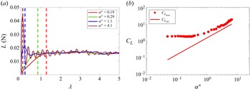


 Open access

