


1. Introduction
Fluctuations in wall pressure induced by turbulent wall-bounded flows can cause structural vibrations and acoustic radiation. Their prediction and an understanding of their fluid dynamic sources are crucial to the reduction of aircraft cabin noise, automobile interior noise, underwater vehicle noise, and noise and vibrations in various other flow systems.
Wall-pressure fluctuations can be split into two components caused by hydrodynamic motions and acoustics (or more generally, compressibility effects). Their wavenumber– frequency spectrum  $\varPhi _{pp}(\boldsymbol {k},\omega )$ is considered to have a shape illustrated schematically in figure 1 as a function of the streamwise wavenumber
  $k_1$ at a fixed frequency
  $\omega$ and the zeroth spanwise wavenumber,
  $k_3=0$ (Blake Reference Blake2017). The hydrodynamic component is peaked at the convective wavenumber
  $k_c=\omega /U_c$, where
  $U_c$ is the convection velocity. The acoustic component is peaked conceptually at the acoustic wavenumber
  $k_0=\omega /c_0$, where
  $c_0$ is the ambient speed of sound, in the limit of diminishing Mach number. The low-wavenumber region before the start of the convective ridge is known as the subconvective wavenumber range that includes the sonic and supersonic wavenumber range,
  $|\boldsymbol {k}| \le k_0$. The latter is responsible for direct sound radiation.
Schematic of the wavenumber–frequency spectrum of wall-pressure fluctuations versus the streamwise wavenumber at a fixed frequency and the zeroth spanwise wavenumber.

In low-Mach-number flows, there is a large length-scale (wavenumber) separation between the convective and acoustic peaks, and the acoustic energy is very weak compared to the hydrodynamic energy, making investigation of the low-wavenumber spectrum a significant challenge both numerically and experimentally. Pressure fluctuations in the subconvective wavenumber range are important practically despite their small magnitude because longer waves are more easily coupled to structural modes to excite vibrations. There is an acute lack of knowledge of their spectral behaviour, particularly with regard to the existence and strength of acoustic peaks and their dependence on the flow Mach number. Acoustic peaks have rarely been measured in experiments, and existing theoretical models predict qualitatively different behaviour at low wavenumbers (see, for example, the review article by Graham Reference Graham1997).
The hydrodynamic component of wall-pressure fluctuations has been studied extensively using incompressible direct numerical simulations (DNS) and large-eddy simulations (LES) (e.g. Kim Reference Kim1989; Choi & Moin Reference Choi and Moin1990; Singer Reference Singer1996; Hu, Morfey & Sandham Reference Hu, Morfey and Sandham2006; Yang & Yang Reference Yang and Yang2022). However, incompressible simulations are incapable of capturing the acoustic contributions. The acoustic component has received only recent attention due to computational difficulties. Commonly used hybrid approaches for aeroacoustics based on acoustic analogy (Wang, Freund & Lele Reference Wang, Freund and Lele2006) are impractical due to lack of separation between source and propagation effects. High-fidelity compressible simulations with high accuracy, high resolution and low dissipation are necessary to capture the weak acoustic signals in wall-pressure fluctuations. Gloerfelt & Berland (Reference Gloerfelt and Berland2013) and Cohen & Gloerfelt (Reference Cohen and Gloerfelt2018) conducted the only studies to date of the acoustic component of wall-pressure fluctuations in subsonic turbulent boundary layers. Through carefully performed LES of flat-plate boundary layers at free-stream Mach number  $0.5$, they identified acoustic peaks corresponding to upstream and downstream propagating waves in the wall-pressure wavenumber–frequency spectra, and investigated their dependence on the mean pressure gradient. However, as they noted, their results were not entirely free of spurious sound from computational boundaries. Artificial noise from numerical boundary conditions is a major obstacle to the study of boundary-layer acoustics, and the problem becomes increasingly severe with decreasing Mach number. Note that at Mach
  $0.5$, the separation between convective and acoustic wavenumbers is limited to a factor of two in Gloerfelt & Berland (Reference Gloerfelt and Berland2013) and Cohen & Gloerfelt (Reference Cohen and Gloerfelt2018).
In the present study, wall-pressure fluctuations are investigated in a plane channel using compressible DNS. With periodic boundary conditions, channel flow provides a clean configuration free of artificial boundary noise, thus facilitating direct computation of flow-generated acoustics at low Mach numbers. This is, to the authors’ knowledge, the first set of DNS that quantifies the acoustic contributions to wall-pressure fluctuations in subsonic channel flow and their Mach number dependence. Simulations are performed at friction Reynolds number  $180$ for bulk Mach numbers
  $0.4$,
  $0.2$ and
  $0.1$, which provide increasingly larger scale separations between the convective and acoustic ridges up to an unprecedented factor of ten. In addition to longitudinal acoustic waves, the present channel-flow simulations also allow an investigation of the obliquely propagating acoustic waves corresponding to various duct modes, and demonstrate the ability of DNS to capture them.
2. Numerical procedure
Turbulent flows in a plane channel are computed using an in-house-developed DNS code that solves the three-dimensional, compressible Navier–Stokes equations in conservative form along with the continuity equation and the equation of state for a calorically perfect gas. The spatial discretization of the inviscid fluxes is based on the locally conservative, non-dissipative finite-difference scheme of Pirozzoli (Reference Pirozzoli2010) to ensure numerical stability without introducing artificial dissipation. The viscous fluxes are discretized based on the scheme of Sun et al. (Reference Sun, Ren, Zhang and Yang2011) to avoid odd–even decoupling. Sixth-order central differencing is employed except for the wall-normal derivatives at the wall and the first and second off-wall points, where fourth-order one-sided, one-side-biased and central differences are used, respectively. The standard fourth-order Runge–Kutta method is adopted for time integration.
A total of five simulations are carried out as summarized in table 1 in terms of the bulk Mach number  $M_b$, computational domain size, number of grid points, and grid spacings in wall units. The main simulations for
  $M_b=0.4$,
  $0.2$ and
  $0.1$ (cases 1–3) are conducted in a computational domain of size
  $16{\rm \pi} \delta \times 2\delta \times 4{\rm \pi} \delta /3$, where
  $\delta$ is the half-channel width, using
  $1024 \times 192 \times 256$ grid points. The grid resolution, with
  $\Delta x_1^+ = 9$,
  $\Delta x_3^+ = 3$ and
  $\Delta x_2^+$ ranging from
  $0.5$ at the wall to
  $3.3$ at the channel centre (
 $\Delta x_2/\eta$ from
  $0.5$ to
  $0.8$ in terms of the local Kolmogorov length
  $\eta$), compares favourably with resolutions in the literature. For
  $M_b=0.4$, two additional simulations are conducted in a shorter domain with
  $L_1=4 {\rm \pi}\delta$ (cases 4 and 5) and with a 50 % grid refinement in each direction (case 5) to examine the domain-length and grid resolution effects. While
  $L_1=4{\rm \pi} \delta$ is commonly used in earlier channel-flow simulations, it is rather restrictive for the long acoustic waves, thus the longer domain with
  $L_1=16{\rm \pi} \delta$ is used as the baseline. The results discussed below are from cases 1–3 unless stated otherwise. In all cases, the friction Reynolds number is
  ${\textit {Re}}_\tau =180$ and the Prandtl number is
  ${\textit {Pr}}=0.72$. No-slip and isothermal boundary conditions are imposed on the walls, and periodic boundary conditions are imposed in the streamwise and spanwise directions. The initial field consists of a parabolic streamwise-velocity profile with random perturbations and uniform density and temperature. Simulations are conducted with
  $\Delta t = 0.005\delta /c$, where
  $c$ is the speed of sound at the wall temperature, corresponding to a CFL limit of
  $1.8$. Statistics are computed based on sampling period
  $250\,\delta /U_b$, or approximately five flow-through times for the long domain, after the flow has become fully developed, which takes approximately twenty flow-through times starting from the initial field.
Simulation Mach numbers, domain and grid sizes, and grid spacings in wall units.

The accuracy of the velocity statistics is demonstrated in figure 2 in comparison with those from the incompressible DNS of Kim et al. (Reference Kim, Moin and Moser1987) using a spectral method, and the DNS of Modesti & Pirozzoli (Reference Modesti and Pirozzoli2016) at  $M_b=0.1$ using a numerical scheme similar to the present one. The two reference simulations were performed in shorter domains, with a focus on flow but not acoustic quantities. Both the mean velocity and turbulence intensity profiles, normalized by the friction velocity
  $u_\tau$, agree well with the previous incompressible and nearly incompressible results because the compressibility effect is small even at the largest Mach number, 0.4, and the agreement is notably better as the bulk Mach number decreases. When the mean velocity is van Driest transformed (not shown), the curves become hardly discernible from one another. The flow is found to be nearly isothermal, with mean-temperature (sound-speed) variations across the channel not exceeding
  $2.8\,\%$ (
 $1.4\,\%$) relative to the wall value for
  $M_b=0.4$, and much smaller for
  $M_b=0.2$ and
  $0.1$.
Comparisons of (a) mean velocity profiles and (b) root mean square (rms) of velocity fluctuations at the three Mach numbers with previous DNS results: blue dotted line,  $M_b=0.4$; green dashed line,
  $M_b=0.2$; red solid line,
  $M_b=0.1$; black dash-dotted line, Kim, Moin & Moser (Reference Kim, Moin and Moser1987); orange dash-dot-dot line, Modesti & Pirozzoli (Reference Modesti and Pirozzoli2016).

To analyse the spectral features of wall-pressure fluctuations, the time series of the fluctuating wall pressure,  $p(x_1, x_3, t)$, is first discrete-Fourier-transformed into
  $\hat {p}(k_1,k_3,\omega )$, and the two-dimensional (2-D) wavenumber–frequency spectrum is calculated as
  $\varPhi _{pp}(k_1,k_3,\omega ) = \langle \hat {p}(k_1,k_3,\omega )\,\hat {p}^*(k_1,k_3,\omega )\rangle /(L_1L_3T)$, where
  $T$ is the sample period, and
  $\langle \,\cdot\, \rangle$ denotes averaging over temporal samples. To obtain statistically converged spectra, the data time series is divided into multiple temporal samples with a
  $50\,\%$ overlap, each corresponding to one flow-through time. A Hanning window is applied to each time segment, and the Fourier-transformed data are then multiplied by
  $\sqrt {8/3}$ to compensate for the energy loss caused by windowing.
From the 2-D wavenumber–frequency spectrum, the one-dimensional (1-D) streamwise wavenumber–frequency spectrum can be calculated as  $\phi _{pp}(k_1,\omega ) = \int \varPhi _{pp}(k_1,k_3,\omega )\,\mathrm {d} k_3$. Both the 2-D and 1-D wavenumber–frequency spectra are examined in this paper. In particular, the 2-D spectrum at the zeroth spanwise wavenumber,
  $\varPhi _{pp}(k_1,k_3=0,\omega )$, is of fundamental importance. The frequency spectrum and streamwise wavenumber spectrum can be calculated by integrating
  $\phi _{pp}(k_1,\omega )$ over
  $k_1$ and
  $\omega$, respectively.
3. Results and discussion
3.1. One-dimensional wavenumber–frequency spectra
Isocontours of the streamwise wavenumber–frequency spectrum,  $\phi _{pp}(k_1,\omega )/(\rho _b^2 U_b^3 \delta ^2)$, where
  $\rho _b$ is the bulk density, and
  $U_b$ the bulk velocity, are shown in figure 3(a) for
  $M_b=0.4$. The corresponding contours for the
  $M_b=0.2$ and
  $0.1$ cases are visually the same. The spectral contours are dominated by the right-tilting convective ridge while no acoustic ridges can be found, indicating that the acoustic contribution is too weak to be delineated in the 1-D spectrum. The dashed line in the figure represents the approximate location of the peak of the convective ridge given by
  $\omega /k_1=U_c$, where
  $U_c$ is the overall convection velocity defined as the value of
  $u$ that maximizes
  $\int \phi _{pp}(k_1,uk_1)\,\mathrm {d} k_1$ (Choi & Moin Reference Choi and Moin1990). In the present case,
  $U_c \approx 0.88U_b$. Note that more precisely, the convection velocity depends on
  $k_1$ and
  $\omega$, thus the precise spectral peak may deviate slightly from the straight line in figure 3(a).
Streamwise wavenumber–frequency spectrum of wall-pressure fluctuations. (a) Isocontours of  $\phi _{pp}(k_1,\omega )/(\rho _b^2 U_b^3 \delta ^2)$ for
  $M_b=0.4$. (b) Plot of
  $\phi _{pp}(k_1,\omega )$ versus
  $k_1$ at selected frequencies for three Mach numbers: dotted lines,
  $M_b=0.4$; dashed lines,
  $M_b=0.2$; solid lines,
  $M_b=0.1$.

To provide a more quantitative view of the spectrum, its values at six selected frequencies are shown in figure 3(b) as a function of  $k_1$ for all three Mach numbers. The effect of Mach number is very small, and there are no acoustic peaks except at the very low frequency of
  $\omega \delta /U_b=1$, suggesting that the acoustic energy is generally weaker than the hydrodynamic energy even at sonic and supersonic wavenumbers. As expected, the hydrodynamic energy is not much affected by the flow Mach number.
To validate the simulation method and evaluate the compressibility effect on the wall-pressure spectra, the present results are compared with the incompressible DNS results of Choi & Moin (Reference Choi and Moin1990). Figure 4(a) shows a comparison of the dimensionless streamwise wavenumber spectra  $\phi _{pp}(k_1)/(\rho _b^2 u_\tau ^4 \delta )$. The compressible DNS results match well the incompressible spectrum. The latter was computed in a shorter domain,
  $L_1=4{\rm \pi} \delta$, and was therefore unable to capture the lowest two wavenumbers in the present study. Similar agreement is observed between the compressible and incompressible frequency spectra, which closely resemble the streamwise wavenumber spectra because the two are known to satisfy Taylor's hypothesis (Choi & Moin Reference Choi and Moin1990).
Spectral comparisons with the incompressible results of Choi & Moin (Reference Choi and Moin1990). (a) Streamwise wavenumber spectrum, (b) streamwise wavenumber–frequency spectrum at  $\omega \delta /u_\tau =262$, for: blue dotted line,
  $M_b=0.4$; green dashed line,
  $M_b=0.2$; red solid line,
  $M_b=0.1$; black dash-dotted line, Choi & Moin (Reference Choi and Moin1990); purple dash-dot-dot line,
  $-1$ slope; orange dash-dot-dot line,
  $-5$ slope.

Figure 4(b) compares the streamwise wavenumber–frequency spectra  ${\phi _{pp}(k_1,\omega )/ (\rho _b^2 u_\tau ^3 \delta ^2)}$ with the result of Choi & Moin (Reference Choi and Moin1990) at frequency
  $\omega \delta /u_{\tau }=262$ (
 $\omega \delta /U_b=16.5$). The compressibility effect is small although discernible, and no acoustic peaks are present. The convective peaks from all cases are in general agreement, and with decreasing Mach number, they approach the incompressible result of Choi & Moin (Reference Choi and Moin1990). However, their spectral curve exhibits a secondary peak at the low-wavenumber end, which they termed ‘artificial acoustics’ since the incompressible simulation could not possibly capture real acoustics. Similar low-wavenumber peaks were also observed in other incompressible studies (e.g. Singer Reference Singer1996; Yang & Yang Reference Yang and Yang2022). The spectra from the present compressible DNS are free of such a secondary peak, suggesting that the ones observed in the literature are indeed numerical artefacts. Additionally, the spectra from compressible simulations decay rapidly with wavenumber at subconvective wavenumbers, whereas the incompressible spectrum flattens out at a significant level, which is likely also a numerical artefact.
3.2. Two-dimensional wavenumber–frequency spectra
Of all wavenumbers, the zeroth spanwise wavenumber of the 2-D wavenumber–frequency spectrum of wall-pressure fluctuations is of particular importance as it corresponds to disturbances travelling along the channel. Isocontours of  $\varPhi _{pp}(k_1,k_3=0,\omega )/(\rho _b^2 U_b^3 \delta ^3)$ for the three Mach numbers are shown in figure 5, where figures 5(d–f) are close-up views of figures 5(a–c) at lower wavenumbers and frequencies. In addition to the convective ridge as in the 1-D spectrum in figure 3(a), distinct acoustic ridges corresponding to various duct modes in the plane-channel flow (Wang & Kassoy Reference Wang and Kassoy1992; Rienstra & Hirschberg Reference Rienstra and Hirschberg2004) are identified, as can be seen most clearly in figures 5(d–f). For sound propagation in a 2-D duct with a uniform flow of Mach number
  $M_b$, the duct modes satisfy (Rienstra & Hirschberg Reference Rienstra and Hirschberg2004)
 \begin{equation} \frac{k_1}{k_a} = \frac{-M_b\pm \sqrt{1-\beta^2q_n^2}}{\beta^2}, \end{equation}
where  $k_a = \omega /c$ is the acoustic wavenumber in the absence of flow,
  $\beta =\sqrt {1-M_b^2}$ is the Prandtl–Glauert parameter, and
  $q_n=n{\rm \pi} c/(2\omega \delta )$. The theoretical predictions of the duct modes for different mode numbers
  $n$ are depicted in figures 5(d–f) as dotted lines. They coincide with the thin ridges outside of the convective ridge, confirming the acoustic nature of these ridges. A closer inspection of the acoustic ridges reveals that energy is concentrated at discrete wavenumbers because the periodic boundary condition imposed over the finite domain length can accommodate
  $k_{1} \delta = 2{\rm \pi} m \delta /L_1$ (
 $= m/8$ for the long domain) only for
  $m$ from
  $- N_1/2$ to
  $N_1/2$.
Contours of  $\varPhi _{pp}(k_1,k_3=0,\omega )/(\rho _b^2 U_b^3 \delta ^3)$ for three different Mach numbers: (a,d)
  $M_b=0.4$, (b,e)
  $M_b=0.2$, (c,f)
  $M_b=0.1$. Here, (d–f) are close-up views of (a–c) in lower wavenumber–frequency ranges. The dotted lines represent the
  $n$th duct acoustic modes predicted by theory, and the dash-dotted line represents the locus of cut-on frequencies for the duct modes.

At  $n=0$, the theoretical phase speeds from (3.1) reduce to
  $\omega /k_1 = U_b \pm c$. They are represented by the two straight dotted-lines in figures 5(a–f) and define the supersonic wavenumber range in between. The acoustic ridges along these two lines correspond to the longitudinal waves propagating in the downstream (rightward) and upstream (leftward) directions. The length-scale (wavenumber) separation between the acoustic and convective ridges grows with decreasing Mach number, resulting in an increasingly smaller supersonic region. The wall-pressure spectral peaks associated with the downstream propagating waves are stronger than those associated with upstream propagating waves, especially at higher Mach numbers. The same trend was observed in the boundary-layer studies of Gloerfelt & Berland (Reference Gloerfelt and Berland2013) and Cohen & Gloerfelt (Reference Cohen and Gloerfelt2018). This is likely due to refraction by the mean-velocity gradient, which channels acoustic energy towards the wall for downstream propagating waves, and away from the wall for upstream propagating waves (Wang & Kassoy Reference Wang and Kassoy1992). Theory predicts that the refraction effect increases with frequency and mean flow Mach number. Both trends are exhibited in the numerical results.
The  $n>0$ modes, corresponding to the curved acoustic ridges in the supersonic wavenumber range, represent the oblique acoustic waves that are reflected repeatedly from the channel walls as they propagate upstream or downstream. The number of oblique modes increases with frequency, and at a given frequency, with the flow Mach number. The cut-on frequency for the
  $n$th mode is the bottom of the curved ridge. Its value, obtained by setting the radical in (3.1) to zero, is
  $\omega \delta /U_b = (n{\rm \pi} /2)(1/M_b^2 - 1)^{1/2}$. The locus of cut-on frequencies for the various duct modes is indicated in the figure by the dash-dotted lines, which separate the upstream and downstream propagating oblique waves. As the flow Mach number decreases, the acoustic ridges at low frequencies become less pronounced but remain identifiable even at
  $M_b = 0.1$. At high frequencies (
 $\omega \delta /U_b \gtrsim 20$), propagating acoustic waves can no longer be identified, but there is a broader rise in spectral level around the sonic lines, particularly the downstream propagating one, forming broader ridges as illustrated in figures 5(a–c). Interestingly, these ridges are more prominent at lower Mach numbers.
In figure 6,  $\varPhi _{pp}(k_1,k_3=0,\omega )$ is plotted against
  $k_1$ at six distinct frequencies for the three Mach numbers. The symbols on the spectral curves correspond to the expected wavenumbers of the upstream and downstream propagating longitudinal waves,
  $k_1=\omega /(U_b\pm c)$. They are in close agreement with the computed peak wavenumbers of the longitudinal waves. Additional peaks corresponding to oblique waves can be seen between the two longitudinal-wave peaks at higher Mach numbers and frequencies, when the frequency exceeds their cut-on frequencies. This figure also demonstrates quantitatively that the wall-pressure spectrum outside the supersonic wavenumber range is virtually independent of the flow Mach number. The pressure spectra in the positive
  $k_1$ range are replotted in figure 7(a) on a log-log scale to allow a closer examination of their low-wavenumber behaviour. It shows that the spectral level of the longitudinal acoustic peak decreases with flow Mach number, and the difference becomes smaller with increasing frequency. At high frequencies, no discernible acoustic peaks exist, and the broadband spectral level in the subconvective range becomes higher at lower Mach numbers, as seen previously in the spectral contours in figure 5. In figure 7(b), the same spectral curves are rescaled such that the spectral level is normalized based on the frequency spectrum
  $\phi _{pp}(\omega )$, and
  $k_1$ is normalized by the convective wavenumber
  $k_c(\omega )$, defined as the peak wavenumber of
  $\phi _{pp}(k_1,\omega )$. This scaling is seen to collapse the convective peaks for
  $\omega \delta /U_b \ge 10$, and align the longitudinal acoustic wavenumbers at various frequencies for a given Mach number. The increasing length-scale separation between the hydrodynamic and acoustic motions with decreasing Mach number is highlighted by the decreasing
  $k_1/k_c$ value of the acoustic peaks.
Wall-pressure spectrum  $\varPhi _{pp}(k_1,k_3=0,\omega )$ versus streamwise wavenumber
  $k_1$ at six selected frequencies for three different Mach numbers: dotted lines,
  $M_b=0.4$; dashed lines,
  $M_b=0.2$; solid lines,
  $M_b=0.1$. The symbols indicate the theoretical longitudinal acoustic wavenumbers:
  $\diamond$,
  $M_b=0.4$;
  $\circ$,
  $M_b=0.2$;
  ${\square}$,
  $M_b=0.1$.

Wall-pressure spectrum  $\varPhi _{pp}(k_1,k_3=0,\omega )$ versus positive streamwise wavenumber
  $k_1$ at six selected frequencies with two different normalizations: (a) same as in figure 6; (b) normalization based on frequency spectrum
  $\phi _{pp}(\omega )$ and convective wavenumber
  $k_c(\omega )$. The different lines represent: dotted lines,
  $M_b=0.4$; dashed lines,
  $M_b=0.2$; solid lines,
  $M_b=0.1$. The symbol on each curve corresponds to the theoretical acoustic wavenumber of the downstream propagating longitudinal wave.

In addition to the zeroth spanwise wavenumber, isocontours of  $\varPhi _{pp}(k_1,k_3,\omega )$ at the first three non-zero spanwise wavenumbers,
  $k_3\delta =1.5$,
  $3$ and
  $4.5$, are shown in figure 8 in the low streamwise wavenumber range for the
  $M_b=0.4$ case. Distinct acoustic ridges are observed clearly. They are associated with propagating waves that are oblique relative to both wall-normal and spanwise directions, with higher cut-on frequencies and slower propagation speeds in the streamwise direction compared to the corresponding zeroth spanwise modes (cf. figure 5d). The acoustic energy decays with increasing spanwise wavenumber. It is worth noting that the convective ridge is relatively unchanged within the spanwise wavenumber range plotted. The
  $M_b=0.2$ and
  $0.1$ cases exhibit the same qualitative behaviour for
  $\varPhi _{pp}(k_1,k_3,\omega )$ but with fewer acoustic ridges (
 $1/2$ and
  $1/4$ of the
  $M_b=0.4$ value), and are omitted here for brevity.
Contours of  $\varPhi _{pp}(k_1,k_3,\omega )/(\rho _b^2 U_b^3 \delta ^3)$ at the first three non-zero spanwise wavenumbers for the
  $M_b=0.4$ case: (a)
  $k_3\delta =1.5$, (b)
  $k_3\delta =3$, (c)
  $k_3\delta =4.5$.

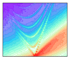
Figure 9 shows contours of  $\varPhi _{pp}(k_1,k_3,\omega )$ in the
  $k_1$–
 $k_3$ plane at three frequencies,
  $\omega \delta /U_b=5$,
  $10$ and
  $15$, for the
  $M_b=0.4$ case. The convective ridge is elongated and slow-varying with respect to the spanwise wavenumber, which explains its relative invariance exhibited in figure 8. The dotted ellipse in each plot indicates the theoretical boundary of the supersonic wavenumber region defined by (Gloerfelt & Berland Reference Gloerfelt and Berland2013):
 \begin{equation} \frac{(k_1+ M_b k_a/\beta^2)^2}{(k_a/\beta^2)^2} + \frac{k_3^2}{(k_a/\beta)^2} = 1. \end{equation}
As can be observed, the supersonic region is very small and hardly separated from the convective ridge at low frequencies. It grows in area and becomes more distant from the convective ridge as frequency increases, and multiple acoustic modes appear within the supersonic region. The modes along the ellipse represent waves propagating parallel to the wall, whereas those inside the ellipse represent waves oblique to the wall. Note that the low-wavenumber resolution of the numerical simulation is significantly lower in the spanwise direction relative to the streamwise direction because  $L_3$ is much smaller than
  $L_1$. Ideally, an equally large
  $L_3$ would be used to provide equal wavenumber resolution in both directions and thereby a better description of the acoustic cone. Nonetheless, the present results provide a meaningful estimate of the significance of the acoustic region in the subconvective wall-pressure spectra, particularly for the zeroth spanwise wavenumber component.
Contours of  $\varPhi _{pp}(k_1,k_3,\omega )/(\rho _b^2U_b^3\delta ^3)$ at three selected frequencies for the
  $M_b=0.4$ case: (a)
  $\omega \delta /U_b=5$, (b)
  $\omega \delta /U_b=10$, (c)
  $\omega \delta /U_b=15$. The dotted ellipse represents the theoretical boundary of the supersonic wavenumber region.

As a measure of the energy contained within the acoustic region, the wavenumber– frequency spectra of the fluctuating wall-pressure for the three Mach number cases are integrated over the supersonic wavenumbers and compared in figure 10. Figure 10(a) depicts the integrated 2-D spectra,  $\phi _{pp,{sup}}(\omega ) = \int _{supersonic}\varPhi _{pp}(k_1,k_3,\omega )\,\mathrm {d} k_1\,\mathrm {d} k_3$, which are related to acoustic waves in all directions. Figure 10(b) shows the spectra for the zeroth spanwise wavenumber integrated over supersonic streamwise wavenumbers,
  $\phi _{pp,{sup}}(\omega, k_3=0) = \int _{supersonic}\varPhi _{pp}(k_1,k_3=0,\omega )\,\mathrm {d} k_1$, pertaining to waves propagating in the
  $x_1$–
 $x_2$ directions only. For each Mach number, the vertical dash-dotted line of the same colour denotes the theoretical cut-on frequency of the first oblique mode. It is observed that the onset of the first oblique duct mode drastically amplifies the energy level, whereas the onset of subsequent oblique modes is hardly noticeable. The oscillations with frequency exhibited by the curves stem from the discrete acoustic wavelengths accommodated by the finite computational domain, as discussed previously. Despite the oscillations, which are most prominent prior to the onset of oblique modes, and somewhat obfuscate the relative magnitudes among the curves, it can be recognized that at lower frequencies, the energy in the acoustic region decreases with flow Mach number, and the difference is magnified by the earlier onset of oblique waves at higher Mach numbers. However, this trend reverses at higher frequencies (
 $\omega \delta /U_b\gtrsim 22$ for
  $\phi _{{pp},{sup}}(\omega )$, and
  $\omega \delta /U_b\gtrsim 19$ for
  $\phi _{{pp},{sup}}(\omega, k_3=0)$), as also observed earlier in figures 5–7. Relative to the total energy in figure 10(a), the energy associated with
  $k_3=0$ waves exhibits weaker Mach number dependence at lower frequencies and a more pronounced trend reversal at higher frequencies. When the spectra in figures 10(a,b) are normalized by their respective spectra integrated over all wavenumbers, the results show that the energy in the supersonic wavenumber range as a fraction of the total energy (dominated by hydrodynamics) is smallest in the mid-frequency range and rises at higher frequencies, as the convective ridge weakens faster with frequency than the acoustic ridges. It should be noted that the pressure fluctuations in the supersonic wavenumber range are not purely acoustic; the hydrodynamic motions of the fluid also make broadband contributions to these wavenumbers. Since the entire channel is both the acoustic source field and the medium of propagation, a separation of acoustic waves from their source processes is a challenge that warrants future investigation.
Wall-pressure spectra integrated over the supersonic wavenumber range for (a) fully 2-D spectrum, and (b) 2-D spectrum at zeroth spanwise wavenumber, for the three Mach numbers: blue dotted line,  $M_b=0.4$; green dashed line,
  $M_b=0.2$; red solid line,
  $M_b=0.1$. The vertical dash-dotted lines represent the theoretical cut-on frequencies of the first oblique mode for the three Mach numbers.

3.3. Grid and domain-size effects
The grid resolution employed in the present DNS is comparable to those of various previous DNS studies in the literature. Nevertheless, since the earlier studies were focused on hydrodynamics only, a grid-convergence study is conducted to assess the accuracy of the acoustic component of wall-pressure fluctuations. Two additional simulations are carried out for  $M_b=0.4$ in a shorter domain on the original and refined grids, cases 4 and 5 respectively, in table 1, and the results are compared in figure 11(a) in terms of
  $\varPhi _{pp}(k_1,k_3=0,\omega )$ at selected frequencies. Although small discrepancies are seen at high wavenumbers, both convective and acoustic peaks are grid-converged at dimensionless spectral levels above
  $10^{-17}$, for over an eleven-decade range. The shorter domain simulation on the original grid also allows an evaluation of the domain-size effect by comparing
 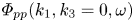 $\varPhi _{pp}(k_1,k_3=0,\omega )$ obtained from the two domains, cases 1 and 4 in table 1. The results, shown in figure 11(b), indicate that even with a factor of 4 difference in domain length, the acoustic peaks are consistent except at near-zero wavenumbers, where they are better resolved by the long domain, as expected.
Wall-pressure spectrum  $\varPhi _{pp}(k_1,k_3=0,\omega )$ versus streamwise wavenumber
  $k_1$ at selected frequencies for
  $M_b=0.4$. (a) Grid-refinement comparison: solid line, original grid; dashed line, refined grid. (b) Domain-length comparison: solid line,
  $L_1=16{\rm \pi} \delta$; dashed line,
  $L_1=4{\rm \pi} \delta$.

Statistical convergence of the wall-pressure spectra is verified through comparisons of results with different sampling times. To double-check independence of the spectra on initial disturbances, which is particularly important given the non-dissipative numerical scheme employed, the  $M_b=0.2$ simulation (case 2) is repeated with two different initial fields: a fully-developed
  $M_b=0.4$ field, and a fully-developed
  $M_b=0.1$ field. The results are virtually identical and agree with that produced by the simulation with random initial disturbances.
4. Conclusion
Wall-pressure fluctuations induced by turbulent channel flow are investigated using compressible DNS at three bulk Mach numbers,  $M_b=0.4$,
  $0.2$ and
  $0.1$, and friction Reynolds number
  $180$, with a focus on the spectral behaviour at subconvective wavenumbers. The results, for the first time to the authors’ knowledge, capture contributions from the propagating acoustic waves including longitudinal and oblique duct modes. The three Mach numbers considered allow increasingly larger separations between hydrodynamic and acoustic length scales. While the acoustic contributions are nearly invisible in the 1-D streamwise wavenumber–frequency spectrum, they are clearly identified in the 2-D wavenumber–frequency spectrum. The acoustic ridges are orders of magnitude weaker than the convective ridge and decay with the flow Mach number in the lower frequency range, but remain distinctly identifiable even at
  $M_b = 0.1$. The longitudinal and oblique acoustic modes compare well with the theoretical predictions of 2-D duct modes with a uniform mean flow. At higher frequencies, propagating acoustic waves are diminished, but the spectral level is broadly elevated in the supersonic wavenumber range, and its variation with Mach number is reversed.
The 1-D streamwise wavenumber–frequency spectra of the fluctuating wall pressure are little affected by the compressibility effect and agree well with previous incompressible DNS results in the convective wavenumber range. They exhibit lower subconvective spectral levels and are free of the ‘artificial acoustics’ peak observed in the incompressible solutions, confirming that the latter is indeed a numerical artefact. It is worth pointing out that although the present study indicates very low acoustic energy overall relative to the hydrodynamic energy in a plane channel, small surface inhomogeneities can cause a drastic increase in acoustic power in real-world applications through acoustic diffraction and turbulence generation (Ji & Wang Reference Ji and Wang2010; Yang & Wang Reference Yang and Wang2013; Devenport et al. Reference Devenport, Alexander, Glegg and Wang2018).
Acknowledgements
M.W. is indebted to William Blake for inspirational discussions. A portion of this work was presented in AIAA Paper 2021-2142, AIAA AVIATION Forum (Virtual Event), 2–6 August 2021.
Funding
This research was supported by the Office of Naval Research under grants N00014-17-1-2686 and N00014-20-1-2687, with K.-H. Kim and Y.L. Young as Program Officers. Computer time was provided by the US Department of Defense High Performance Computing Modernization Program.
Declaration of interests
The authors report no conflict of interest.


 Open access