


Introduction
Surprising asymmetries referred to as ‘spokes’ are known to arise in the numerical solutions of thermomechanically coupled ice-sheet flow (Reference Payne and BaldwinPayne and Baldwin, 2000; Reference PaynePayne and others, 2000; Reference HindmarshHindmarsh, 2004, Reference Hindmarsh2006; Reference Saito, Abe-Ouchi and BlatterSaito and others, 2006). In this paper we clarify some of the numerical difficulties in shallow ice-sheet modelling which make the interpretation of these spokes difficult.
While wishing to clarify the spokes problem in a pragmatic manner, we are also intrinsically interested in demonstrating agreement between the results of a standard numerical scheme and the predictions of the continuum model. Indeed, such verification of numerical schemes (Reference RoacheRoache, 1998; Reference Bueler, Lingle, Covey and BowmanBueler and others, 2005) is a desirable step for ice-sheet modelling because validation (comparison of numerical results with observed ice flow) is relatively difficult. Glaciologists cannot completely observe the actual flow, temperature and basal fields required to validate numerical ice-sheet models. (Compare this situation with that of shallow-water modellers using wave tanks, for example.)
At issue are the numerical solutions of a partial differential equation (PDE) free boundary problem, namely the thermomechanically coupled, cold (not polythermal; cf. Reference GreveGreve, 1997) shallow-ice approximation (SIA) (Hutter, 1983). In this continuum model, detailed in the following section, all stresses are neglected with the exception of shear stresses in planes parallel to the geoid. This model is the same continuum model used in the important intercomparison experiments described by Reference PaynePayne and others (2000), referred to here as EISMINT (European Ice Sheet Modelling INiTiative) II.
Our tools for assessing numerical results are exact solutions of the whole problem, which includes all equations, all coupling terms and all boundary conditions. The exact solutions are described and illustrated in the Exact Solutions section. A complete derivation of the exact solutions derivation is given in a separate technical report (Reference Bueler and BrownBueler and Brown, 2006), as are computer codes to compute the exact solutions. It is envisaged that they can be incorporated into ice-sheet codes for routine verification purposes, as they have been for our group.
In Results we use these solutions to verify, for the first time, a numerical scheme for fully thermomechanically coupled ice sheets. We have chosen to verify a particular finite-difference scheme, described in Appendix A, but many other numerical schemes are likely to perform equally well (or better) and can be verified by the same means. We satisfy the usual standard for verification by comparing numerical results with exact solutions in situations which exercise all terms (Reference RoacheRoache, 1998) and, in particular, all thermocoupling mechanisms. For verification, we use both a steady-state and a time-dependent exact solution. Clear evidence of convergence of the numerical solutions to the exact continuum values under grid refinement is found.
The application of our code to EISMINT II experiment F is also described in Results. Spokes are observed in the basal temperature field even though the continuum problem has angular symmetry. In other words, although verification is accomplished for the numerical scheme, there remain initial/boundary value problems for which the numerical results are significantly far from the continuum solution. This situation is interpreted in Analysis and Discussion.
The continuum ice-sheet model used here consists of two evolution-in-time PDEs: one for mass conservation and one for conservation of energy (see following section). Approximations of the decoupled versions of these equations are, naturally, better understood. For instance, numerical schemes for solving the isothermal shallow problem can be verified by the methods described by Reference Bueler, Lingle, Covey and BowmanBueler and others (2005). The stability of several numerical schemes for the isothermal problem has been studied by Reference Hindmarsh, Payne, Hooke and HutterHindmarsh and Payne (1996) and Reference Hindmarsh, Straughan, Greve, Ehrentraut and WangHindmarsh (2001). On the other hand, the numerical analysis of linear advection–conduction equations such as the decoupled temperature equation is relatively well understood. In particular, a finite-element method for the decoupled temperature equation for ice sheets, with a non-linear source term corresponding to strain heating, is carefully described and, to a limited extent, verified by Reference Calvo, Durany and VazquezCalvo and others (1999). A semi-coupled finite-element approximation, with moving upper surface, is carefully analyzed by Reference Calvo, Durany and VazquezCalvo and others (2002a).
One benefit of our verification is the ability to clearly identify and separate the numerical issues affecting the ice-sheet modeller. Since these issues have not been sufficiently identified in the literature, we list them below and expand upon them in the Analysis.
-
1. The equilibrium grounded margin of an ice sheet always has infinite gradient. In the isothermal case, the inevitable numerical consequences of this fact are explored by Reference Bueler, Lingle, Covey and BowmanBueler and others (2005), and those consequences also apply to the thermomechanically coupled case. We believe, for reasons which remain poorly understood, that the geometry of thermomechanically coupled margins is intrinsically more difficult to approximate than the geometry of isothermal margins. Purely numerical techniques, ones not used to produce the results in this paper, may significantly improve numerical approximation of margins in the thermomechanically coupled case (Reference Saito, Abe-Ouchi and BlatterSaito and others, 2007).
-
2. A ‘diffusivity’ can be assigned to the mass conservation equation, in both the thermomechanically coupled and isothermal cases. (See Analysis for a precise definition.) Its magnitude controls stability and maximum time-step for an explicit numerical scheme (Reference Hindmarsh, Straughan, Greve, Ehrentraut and WangHindmarsh, 2001). In particular, the longest allowed time-step for an explicit scheme to maintain stability is one inversely proportional to the maximum of this diffusivity. The time-step is also proportional to the square of the spatial step. Inclusion of implicitness in the numerical treatment of the equation largely resolves this problem, but explicit methods are also effective, especially when adaptive time-stepping is used. Here, we verify an explicit scheme.
-
3. Large numerically computed velocities, especially large vertical velocities arising through incompressibility from rapidly varying (in space) horizontal velocities, can cause the temperature equation to be overly dominated by vertical advection. The primary numerical consequence is that the temperature time-step must be reduced to maintain a good approximation of advection; this is the Courant-Friedrichs-Lewy (CFL) condition for advection (Reference Morton and MayersMorton and Mayers, 2005).
-
4. The mass conservation and temperature equation are nonlinearly coupled. This is due to the temperature dependence in the flow law for ice and the strong dependence of the strain-heating term in the temperature equation on the geometrically determined effective shear stress. This feedback drives an instability which can create spokes in near-basal temperatures. They are seen in angularly symmetric (Reference PaynePayne and others, 2000) and rectangular (Reference Payne and DongelmansPayne and Dongelmans, 1997) cases. In terms of numerical analysis, these spokes are diagnosed as errors caused by large derivatives, with respect to the temperature, of the strain-heating term. A precise error analysis of our finite-difference scheme supports this conclusion (Appendix B). On the other hand, and without any contradiction, these spokes are also a property of the continuum dynamical system itself. In particular, as described in the Discussion, the continuum problem experienced by the EISMINT II experiment F set-up is believed to have an unstable (repelling) equilibrium solution.
The numerical issues described above differ in detail among numerical schemes, but we believe issues (1), (3) and (4) are universal among finite-difference and finite-element schemes, while (2) applies at least to all explicit time-stepping schemes. The techniques of this paper deal in practical ways with all of these issues.
From one point of view, the above issues all address numerical errors, that is, numerical results which differ from the generally unknowable predictions of the differential equations themselves. It is possible for numerical schemes which take excessively long time-steps to experience numerical instabilities, numerical errors in which small irregularities of the gridded values (‘wiggles’) grow exponentially. In the current non-linear circumstances it is possible for such wiggles to grow to bounded maximum magnitude, though they may grow exponentially at small magnitude. This can happen for implicit and semi-implicit schemes (Reference Hindmarsh, Payne, Hooke and HutterHindmarsh and Payne, 1996) which would be unconditionally stable when applied to linear differential equations. On the other hand, bad margin approximation, issue (1) above, is an example of a stable numerical error of large magnitude.
A deeper issue is whether the thermomechanically coupled SIA can be regarded as a trustworthy continuum mathematical problem. This question is an area of active research (Reference HindmarshHindmarsh, 2004, Reference Hindmarsh2006; Reference Saito, Abe-Ouchi and BlatterSaito and others, 2006). The verification results of this paper, as well as the spoke-free results from many numerical codes for the better-behaved EISMINT II experiments (e.g. experiments A, B, C, D, E and G, in particular), give strong evidence that for many initial/ boundary value problems and for equations with additional source terms this continuum model can be effectively approximated by numerical schemes. In fact, as described in the Discussion, we find no clear evidence that the time-dependent thermomechanically coupled SIA is ill-posed.
As noted, we do observe that the spokes of EISMINT II experiment F strongly suggest an unstable equilibrium point of the continuum dynamical system. Furthermore, as addressed in the Discussion, it may be the case that the equilibrium thermomechanically coupled SIA is ill-posed in EISMINT II experiment F circumstances, but only in the sense that the solution of the continuum problem is not a continuous function of the data of the problem (accumulation, bed elevation and surface temperature).
Clear identification of the sources and nature of numerical errors is critical to the assessment of increasingly sophisticated codes which approximate the many coupled continuum processes in ice flow. Identification and understanding of errors can only occur using reasonably precise tools, and this is one value of exact solutions. An additional practical benefit is that if a suite of exact solutions are available during the code development process, then the effect of various numerical choices and changes may be immediately assessed. One can determine whether a change puts the numerical results closer to or further from the continuum solution. This situation contrasts strongly with the use of the results of intercomparison exercises as ‘benchmarks’.
Continuum Model
The flat-bed, non-sliding base case of the (cold) SIA is, for the purposes of this paper, taken to be the following pair of evolution-in-time PDEs:


Here H(t, x, y) is the ice-sheet thickness and T(t, x, y, z) is the ice temperature. Coordinates x, y, z form a Cartesian system with z positive above the flat base at z = 0. Here and in all of the following, the dot product, gradient and divergence are in the horizontal variables only. Also, (a, b) will denote a two-component vector, so ∇f = (∂f/∂x, ∂f/∂y) and ∇ · (a, b) = ∂a/∂x + ∂ɓ/∂y. The remaining notation in Equations (1) and (2) is listed with values of physical constants in Table 1. Our notation matches that of EISMINT II when possible.
Notation and units for functions and constants used in the construction of exact solutions tests F and G

The first of the above equations enforces mass conservation in the map plane, and the second is the shallow approximation of conservation of energy. These two evolution equations are coupled by the following relations and definitions:






The vector (σ xz , σ yz ) represents the non-negligible part of the deviatoric stress tensor in the SIA. The effective shear stress σ is the length of this vector, so by Equation (3),

The constitutive relation

relates the strain rate tensor  to the deviatoric stress tensor σij
by the scalar factor F(T, σ) which we specify in Equation (4).
to the deviatoric stress tensor σij
by the scalar factor F(T, σ) which we specify in Equation (4).
We use Glen’s exponent n = 3 throughout this paper. Note that the form of the constitutive relation Equation (10) allows much more general dependence on temperature and effective shear stress than the chosen Arrhenius–Glen form in Equation (4). However, we will employ Equation (4) for the construction of exact solutions.
The physics included in thismodel is described by Reference PatersonPaterson (1994), among other sources. A derivation from the Stokes equations for slowfluid flow, including the appropriate smallaspect-parameter shallowness argument, is provided by Reference FowlerFowler (1997). This model is referred to as the SIA in this paper and elsewhere (Hutter, 1983).
Some additional comments on the above equations can be made. The horizontal ice flux Q = Q(t , x, y) can be represented 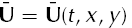 if is the average horizontal velocity in each column. Equation (5) can be derived from the constitutive relation by vertically integrating the nonnegligible components of the strain rate tensor. The vertical velocity w(t , x, y, z) is found, as described in Equation (7), by vertically integrating the incompressibility equation
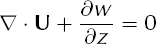
and setting w = 0 at the frozen base of the ice on a stationary bed. Equations (1), (6) and (7) imply

which is referred to as the surface kinematic equation. Indeed, Equation (1) is equivalent to Equation (12) in the coupled system. Finally, note that Equations (2), (3), (5) and (8) all incorporate shallowness assumptions.
Regarding conservation of energy, Equation (2), we have assumed that the ice is cold and that no liquid is present in the ice lattice, so the ice is not polythermal (Reference GreveGreve, 1997). As is standard in the SIA, we include both advection and conduction terms in the vertical direction but neglect conduction of heat in the horizontal direction (Reference FowlerFowler, 1997).
Quantities σ, U, w, Q, Σ and F(T , σ) can all be eliminated. Thiswould reduce the systemof equations (1), . . . , (9) to only two equations for the evolution of H and T. This would not improve clarity, but one might say that the resulting coupled systemof two scalar evolution equations is the systemthatwe are actually solving. These two equations would be integrodifferential equations because velocities are built from integrals of the z-dependent temperature function.
It is by no means true that the above system incorporates all features of existing ice-sheet models. Most existing codes based upon the SIA include additional continuum processes (polythermal ice, bedrock heat storage, bed deformation, coupling to ice shelves, etc.). Evidently, such models exhibit even more complex dynamics. Verification of a numerical scheme for the continuum model in this paper is not sufficient to verify numerical schemes for those complex models.
Some ice-sheet models include more elaborate, or simply different, stress balances than are included in the SIA. These models, which are based on the full Stokes system or on other shallow approximations thereof (Reference MacAyealMacAyeal, 1989; Reference BlatterBlatter, 1995), cannot be meaningfully verified using the exact solutions of this paper. These other continuum models must evidently be verified using exact solutions of the relevant equations. For example, Reference SchoofSchoof (2006) describes a non-trivial exact solution to the equations for an isothermal ice stream with purely plastic till.
Note that a simplification of the continuum model described here is the isothermal shallow-ice equation, a single PDE for thickness H. It is derived from Equation (1) by supposing a constant temperature in Equation (5). The flat-bed result, after eliminating σ, U and Q, may be written

where A 0 is a softness parameter corresponding to a constant temperature.
Boundary conditions
PDEs (1) and (2) require boundary and initial conditions to complete a (presumed) well-posed mathematical problem.
Because the margin is allowed to move, the boundary condition for Equation (1) used here (and in Reference Bueler, Lingle, Covey and BowmanBueler and others, 2005) is

which is really a constraint on the allowed thickness functions. In fact, it is essential to note that Equation (1) is solved (in general) as a free boundary problem. The map-plane region covered by ice is not predetermined. This free boundary problem is known to be well posed in the isothermal case (Reference Calvo, Dſaz, Durany, Schiavi and VasquezCalvo and others, 2002b). In particular, it is shown by Reference Calvo, Dſaz, Durany, Schiavi and VasquezCalvo and others (2002b) that at a free margin where H = 0 the flux Q is also zero in the correctly (weakly) formulated mathematical problem including inequality (14). Finding the location of the margin is part of the problem. To make up for the added unknown boundary location, at the boundary both the thickness and the flux are equal to zero. (These would be overdetermined boundary conditions if they were regarded as boundary values for a PDE in the classical sense.)
A numerical approximation of this free boundary problem is available in an appropriately formulated finite-element method (Reference Calvo, Dſaz, Durany, Schiavi and VasquezCalvo and others, 2002b). A principled approximation is much less clear for a finite-difference method such as the one used here. That is, it is harder to know in advance that a given finite-difference approximation treats the moving margin boundary condition correctly. We note, however, that straightforward enforcement of inequality (14) at each time-step and at each point of the finite-difference grid gives verifiably reasonable results in the current paper and in the isothermal case (Reference Bueler, Lingle, Covey and BowmanBueler and others, 2005).
The three-dimensional (3-D) region on which Equation (2) applies varies in time, but the boundary conditions are of the classic type. On the upper surface of the ice,

where r 2 = x 2 + y 2 and (x, y) = (0, 0) is taken to be the center of the angularly symmetric ice sheet. In this paper, as in EISMINT II, the surface temperature is a specified function of the map-plane position. For construction of exact solutions (below) we take T min = 223.15 K, the value used in experiment F of EISMINT II. Note that experiment F has the strongest basal temperature spokes of the EISMINT II nonsliding base experiments. (See Table 1 for values of constants not discussed in the text.) A constant geothermal flux is applied at the base of the ice, z = 0:
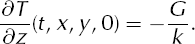
There is no bedrock thermal model.
Exact Solutions
The differential equations describing ice flow are complicated and highly non-linear. It is generally correct to say that they do not possess exact solutions that can be computed by hand. More precisely, for arbitrary initial/boundary values and arbitrary source functions it is rare to find analytical solutions. (By ‘source functions’ we mean known functions which appear additively as terms in the differential equations. The accumulation M in the ice flow Equation (1) is a source function.)
If, however, one seeks an exact (analytical) solution only for the purpose of testing the accuracy of a numerical code, there is hope for producing such solutions. One idea, implemented in this section, is to choose reasonable solution functions, in this case analytical functions of time and space for ice thickness and temperature. Source functions are then adjusted to accommodate the chosen solution functions. One thereby makes the chosen functions into actual solutions. Reference RoacheRoache (1998) refers to this general technique as the ‘method of manufactured solutions’.
For instance, in the isothermal case, Equation (13) can be used to determine the accumulation function M given a choice for H; Reference Bueler, Lingle, Covey and BowmanBueler and others (2005) call such M ‘compensatory’. One can test a code for approximating Equation (13) by comparing the numerical thickness to the chosen exact thickness function. In particular, the exact compensatory accumulation M is used at each time-step during the numerical run, while the exact thickness is used as the initial condition and at the end of the run to evaluate the accuracy of the numerical thickness.
To manufacture solutions in the thermomechanically coupled case, we must replace Equation (2) with a more general form incorporating an additional heat source (denoted Σc):

By adding a term to Equation (2) we are solving a more general version of the conservation of energy. The reader may interpret Equation (17) as modelling ice in which a chemical reaction is occurring, either endo- or exothermic according to the sign of Σc, for instance.
We have already made two other modifications of the standard SIA model to allow the manufacture of exact solutions. These modifications, which are less significant than the addition of a source term in Equation (17), are: (i) the constitutive relation (4) used for the exact solutions in this paper is of simple Arrhenius–Glen–Nye form with constant A and Q; specifically we use the cold part of the Paterson–Budd relation (1982); and (ii) the temperature T used in Equation (4) is the non-homologous (absolute) temperature.
We then adopt the following strategy for manufacturing a solution to the simultaneous equations (1), (1 7), (3),..., (9): Once H and T are chosen, the coupling quantities σ, U, w and Σ are determined by the appropriate equations (3),..., (9). The compensatory heat source Σc is then calculated as the quantity necessary to make Equation (17) true. Likewise, a compensatory accumulation function M is determined, through the full system, as the quantity which makes Equation (1) true.
Note that the continuum model has precisely two evolution-in-time equations: Equations (1) and (17). This means that we have the flexibility to adjust two source functions, M and Σc, to allow arbitrary chosen functions H and T to be a solution of the system. Because the thermomechanically coupled system involves both partial derivatives and integrals, however, our procedure for computing M and Σc involves both manual differentiation and integration. The need for exact manual integration, in particular, constrains the form of our flow law and our choice of analytical forms for H and T; see below.
A universal caveat about manufactured solutions is that the computed source functions – the accumulation M and the heat source Σc in our case – are not physical. This caveat does not strongly affect verification of numerical codes, fortunately. Note, furthermore, that if one can find expressions for H and T close to a physical solution then M will be close to physical and Σc will be close to zero. Complicated forms for H and T will, however, inevitably yield difficult manual or computer algebra system calculations when one uses the equations to compute the source functions. The increased potential for error in these calculations may reduce the utility of the exact solutions for the purpose of verification.
Chosen thickness and temperature functions
We calculate two angularly symmetric exact solutions, denoted tests F and G, which are proposed additions to the suite of exact solutions in Reference Bueler, Lingle, Covey and BowmanBueler and others (2005). Test F is a steady-state solution and test G is a time-dependent perturbation of that steady state. The following solution is described as time-dependent, that is, we describe test G. The derivation of test F is a strict simplification.
We also restrict ourselves, in the remainder of this section, to the angularly symmetric case; cylindrical coordinates r =  and z are used. The numerical computations in Results are all on a Cartesian grid, however.
To be reasonably physical, we choose H = H(t, r) based on an angularly symmetric steady-state solution of the isothermal Equation (13), namely the test D thickness function from Reference Bueler, Lingle, Covey and BowmanBueler and others (2005):

where s = r/L. Here r = L is the (constant) location of the margin. This function solves a steady-state version of Equation (13) as shown in Reference Bueler, Lingle, Covey and BowmanBueler and others (2005).
The profile given by Equation (18) is a smooth function of r. The smoothness of H s(r) is important because of the derivative-intensive exact calculations which (eventually) yield the compensatory accumulation M and heat source Σc.
Next, we define a perturbed thickness function

where, concretely,
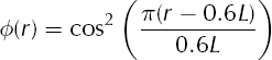
if 0.3L < r < 0.9L while φ(r) = 0 otherwise, and

The term +φ(r)γ(t) is an annular perturbation with amplitude A p and period t p. It also appears in isothermal test D (Reference Bueler, Lingle, Covey and BowmanBueler and others, 2005).
For the steady-state solution test F, we will choose A p = 0 so the perturbation vanishes. For test G we set A p = 200 m and t p = 2000 years. In particular, our choice of A p in test G is small enough so that ∂H/∂r is always negative for all r and t; a consistent sign for ∂H/∂r is convenient in the computation of compensatory sources.
Next, we define the temperature field for the exact solutions test F and G by

where ν is found from H and T s by

Then T satisfies boundary conditions (15) and (16), that is, T = T s at the surface and ∂T /∂z = –G/k at the base.
Illustrations and comments
Figure 1 shows a radial section of the test F ice sheet defined by Equation (19) with temperature field defined by Equation (22). Figure 2 shows the same quantities for test G at t = 500 years, that is, at one-quarter of the perturbation period tp when the perturbation has maximum magnitude.
Thickness and temperature field (K) in test F.

Thickness and temperature field (K) in test G, evaluated at t = 500 years.

Equation (22) defines a vertical temperature profile which (unfortunately) is not very realistic. Note that the ice warms as one goes from the surface to the bed, but the magnitude of ∂T/∂z is relatively constant in each column of ice and there is no horizontal advection bulge in the temperature contours.
The compensatory heat source Σc, derived from H and T via the full thermomechanically coupled system, is non-zero and thus also non-physical. In fact, Σc is larger in magnitude than Σ, though the maximum magnitudes of these functions are within a factor of five.
Because our particular continuum model has a simple Arrhenius term in the constitutive relation (4), and because we do not impose T ≤ T pmp, where T pmp is the pressuremelting temperature, we restrict ourselves to cold ice. This is achieved by using a relatively cold surface temperature (the EISMINT II experiment F surface temperature condition, with a range 223 K < T s < 235 K) and a relatively thin sheet (with dome height H 0 = 3000 m compared to H 0 = 3600m in EISMINT II). It follows from Equations (22) and (23) that 223 K < T < 273 K for all points in the ice; see Figures 1 and 2.
A crucial technical point is that T(t , r , z) in Equation (22) satisfies the boundary conditions (15) and (16) and possesses the property that the integrals for horizontal velocity, flux and vertical velocity can be computed analytically. Specifically, because integrals of the form ∫ ez zn dz can be expressed in terms of elementary functions, and because of the form of the Arrhenius term, we see that functions T with z dependence of the form 1/(C+z) are convenient for purposes of analytical computation. In fact, the integrand in the expression for horizontal velocity (see Equations (4) and (5)) takes the form ez zn multiplied by a complicated z-independent factor. Thus, the integrals (5), (6) and (7) can each be computed exactly. These admittedly technical issues explain choices (22) and (23).
Interestingly, T defined by Equation (22) satisfies
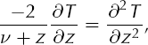
and thus it can be regarded as having a steady-state profile generated by vertical conduction and downward (vertical) advection with a hypothetical vertical velocity w
hyp =  . This may suggest some measure of physical reasonableness, but W
hyp is not the vertical velocity w in the solution which follows. Indeed, T satisfies Equation (17) by design while it satisfies Equation (24) incidentally.
. This may suggest some measure of physical reasonableness, but W
hyp is not the vertical velocity w in the solution which follows. Indeed, T satisfies Equation (17) by design while it satisfies Equation (24) incidentally.
The substitution of H and T into Equations (3) and (5), respectively, and use of the constitutive relation (4), gives analytical formulae for effective stress σ and horizontal velocity U. Taking the horizontal divergence of U and vertically integrating the result (see Equations (6) and (7)) gives analytical formulae for the vertical velocity w and for the term ∇ · Q in Equation (1). Substitution of H and ∇ · Q into Equation (1) gives an analytical formula for the compensatory accumulation M. Substitution of T, U and w into Equations (8) and (17) gives an analytical formula for the compensatory heat source Σc.
The formulae derived for M and Σc have the following property. If Equations (1), (17) and coupling relations (3–8) are solved using the initial values found from the exact H and T, and if the derived formulae for M, Σc are used as accumulation and heat source for the whole coupled system during the solution, then H in Equation (19) and T in Equation (22) solve the whole initial/boundary problem. The previous sentence is at the heart of the matter: we have used the continuum model to find, from chosen H and T, the functions U, w, M, Σ and Σc so that all of the coupled equations are simultaneously true. As long as we believe in the uniqueness of solutions of the continuum problem, then we have the exact solution to that problem. We have manufactured a continuum truth against which to compare numerical approximations. In the following section, we will perform such a comparison against the result of a finite-difference scheme.
The calculations summarized above are both tedious and non-trivial, but their detailed form appears in Reference Bueler and BrownBueler and Brown (2006). We can, however, communicate many of the essential features of the exact solutions by illustrating the various coupling quantities in the thermomechanically coupled system: Figures 3–7 show test F, and Figures 7–9 show test G at time t = 500 years.
Magnitude |U| (m a-1) of horizontal velocity in test F; the vector field U points in the positive r direction.

Vertical velocity w (ma–1) in test F.

Strain heating Σ(10–3 Ka–1) in test F.

Compensatory heating term Σc (10–3 Ka–1) in test F.

Compensatory accumulation M(m a-1) in test G (solid line) at time t = 500 years and in test F (dashed line). The equilibrium radius for test F is r = 403.6 km.

Magnitude |U| of horizontal velocity (m a–1) in test G at time t = 500 years.

Strain heating Σ(10–3 Ka–1) in test G at time t = 500 years.

In some of these figures the margin is not shown. This is in order to avoid division by zero. All quantities H, T, U, w, Σ, Σc and M are bounded all the way to the margin, but in some cases the formulae have 0/0 limits at the margin (Reference Bueler and BrownBueler and Brown, 2006). Numerical errors which might arise by numerically evaluating the exact formulae near these 0/0 limits are avoided in the illustrations here. Similarly, evaluating the exact formulae very close to the (exactly known) location of the margin can and should be avoided when the exact solutions are used for verification. In particular, one should check that a gridpoint is at least a few meters inside the exact margin r = L before evaluating the exact solutions at that gridpoint, in order to determine the numerical error there.
Results
Verification
The exact solutions described above were specifically designed for the purpose of verification. The verification procedure described next is permanently built into our comprehensive ice-sheet model PISM (https://gna.org/projects/ pism/). When we make code changes we redo verification to determine whether numerical results are still close to continuum values.
The data presented here involved substantial grid refinement and represent many thousands of processor hours, but use of exact solutions tests F and G for basic verification should be within the resources of all ice-sheet modelling groups.
We briefly summarize our scheme in Appendix A. The reader not interested in the details of the scheme or in reproducing these results need not read Appendix A but should note that we use an explicit finite-difference scheme for Equation (1), with Reference MahaffyMahaffy (1976)-type evaluation of the diffusivity (see also method 2 in Hindmarsh and Payne, 1996). Furthermore, we use a semi-implicit and first-order upwinded scheme (Reference Morton and MayersMorton and Mayers, 2005) with equal spacing in the vertical, for Equations (2) and (17). Roughly speaking, our scheme uses the simplest consistent choices. The local truncation error (Reference Morton and MayersMorton and Mayers, 2005) of our scheme for Equation (1) is O(Δx2, Δy2, Δt) while the local truncation error for our temperature scheme is O(Δx, Δy, Δz, Δt); see Appendix B. A major purpose of this paper is to quantify the ways in which actual numerical errors for the coupled free boundary problem relate to these local errors.
To verify our thermomechanically coupled SIA scheme using tests F and G, we initialize with the exact continuum values of all quantities and run the code using the exact values of the compensatory accumulation M and heat source Σc at every step. The quantities H, T, u, v, w and Σ are computed numerically at each time-step, and no reference is made to their exact values after initialization except to measure errors at the end of the run. Boundary conditions are held to their exact values at every step. Of course, the numerical solution gradually diverges from the exact values; the results below describe this quantitatively.
The runs reported here were for a fixed time of 25 kyr. This was sufficient time for the scheme to diverge measurably from the exact values. As the exact values are known, there is no reason to run to numerical equilibrium, by whatever standard might be determined. Instead, the actual errors were computed at the final time. Our verification results would not have been significantly different if we had run all computations for 200 kyr.
All runs were completed with adaptive time-stepping, with maximum time-step ▽t limited to 10 years. In particular, Δt satisfied both constraints (25) and (27) at each step; see Analysis below. (Inequality (25) was the active constraint because the maximum velocities in tests F and G are relatively modest. By contrast, the computations of EISMINT II experiment F reported below were affected by both constraints.)
We use a computational ‘box’ with dimensions 1800 km × 1800 km × 4000 m. For example, a spatial grid with spacing Δx = Δy = 10 km and Δz = 40 m corresponds to a threedimensional grid with 181 × 181 × 201 ≈ 6.6 × 10⁶ points. Note that our simple scheme has equal spacing in the vertical (Appendix A).
Our first use of test F for verification is to refine the horizontal grid, namely to use Δx = Δy = 30, 15, 10, 7.5 and 5 km, and to consider thickness errors. Figure 10 shows that there is reasonable decay, under horizontal grid refinement only, of average and dome thickness errors. (Various Δz in the range 6.7–80 m were used to produce Figure 10. The role of Δz is addressed next.) This experiment gives an apparently disappointing result for maximum thickness error, however, as refinement produces maximum thickness errors which are all in the range 25–29 m. These maximum errors do not significantly reduce with refinement (not shown).
Average and dome thickness errors for test F. Several values of Δz were used for each horizontal refinement level; see text.

The maximum thickness and temperature errors always occur in the vicinity of the inevitably poorly approximated margin (Reference Bueler, Lingle, Covey and BowmanBueler and others, 2005). As discovered by Reference Calvo, Dſaz, Durany, Schiavi and VasquezCalvo and others (2002b), however, the quantity η = H(2n+2)/n = H 8/3 is much better approximated than the thickness H itself because η has a bounded gradient at the margin. As shown in Figure 11, the maximum error in η converges at a reasonable rate under purely horizontal grid refinement. For clarity we report the relative maximum of η, that is, max |η∏um _ ηexact\/η exact.
Maximum relative error of η = H 8/3 in test F. Convergence under grid refinement is clear and occurs at a reasonable rate. Several values of Δz were used for each horizontal refinement level.

The grid refinement study reported in Figures 10 and 11 was carried out with several choices of Δz in the range 6.7–80 m. Thickness errors depend weakly on Δz. We can expect temperature errors to depend on the size of Δz, however. If Δx = Δy = 10 km are fixed and Δz is reduced steadily from 80 m to 6.7 m then the average temperature error in test F falls steadily from 0.12 to 0.02 K (not shown).
Clearly grid refinement is a 3-D matter. Instead of reassessing test F in this light, we turn to test G which is time-dependent and therefore of greater interest anyway.
For test G we chose a fixed 3-D refinement path Δx = Δy = 1800/N km and Δz = 4000/N m with N = 60, 90, 120, 180, 240 and 360. In particular, Δx ranges from 30 km down to 5 km while Δz ranges from 66.7 m down to 11.1m. The time-step Δt is limited to 10 years in all runs, but this constraint is only active in the Δx = 20, 30 km cases since for finer grids the time-step was further reduced by adaptive time-stepping (constraints (25) and (27); see Analysis).
We observed reasonable convergence of all the quantities measured. The convergence is predictable for the part of the refinement path with Δx ≤ 15 km. The observed rates O(Δx1’90) and O(Δx1.98) in Figures 12 and 13, respectively, for the average thickness and relative maximum η errors, are essentially optimal for our O(Δx2) local truncation error scheme for the mass conservation equation (Reference Morton and MayersMorton and Mayers, 2005). In fact, given that there is a free boundary problem for thickness, with margin location not determined in advance, these rates are remarkably good.
Average and dome thickness errors for test G. In this and the following two figures the horizontal and vertical grids are simultaneously refined. Rate of convergence given for Δx ≤ 15 km runs.

Maximum relative error of n = H8/3 in test G.

The horizontal location of the margin is at best approximated up to O(Δx) error (Reference Calvo, Dſaz, Durany, Schiavi and VasquezCalvo and others, 2002b; Reference Bueler, Lingle, Covey and BowmanBueler and others, 2005), but this rate is hard to observe because the location of the margin is discrete. There either is or is not ice at a given gridpoint.
Figure 14 shows the numerical errors in temperature using test G. Note that the thickness error made at a single point, namely the dome, and the temperature error at a single point, under the dome at the base, can be somewhat unpredictable. Reports of average and maximum errors are more meaningful.
Temperature errors for test G.

It is believed that Figures 12–14 are the strongest possible indication that we have chosen and correctly coded an effective thermomechanically coupled scheme. In the continuum circumstances of tests F and G, grid refinement produces good agreement between the numerical result and the continuum solution, as well as good rates of convergence.
The angular symmetry of the basal temperature map is of obvious interest. It is shown for test G at the end of a 200 kyr model run with Δx = 30 km in Figure 15. There is no significant angular asymmetry even on this rough grid, and grid refinement clearly reduces the asymmetry. Figure 14 already addresses angular symmetry because the maximum temperature error is less than 2 K at every point in the 3-D domain of ice (for all levels of refinement). This shows that spokes of greater angular variation than 2 K cannot exist, as the reported error compares the numerical result to the exact and angularly symmetric solution to the continuum problem.
Basal temperatures in test G at 200 kyr with Δx = Δy = 30 km and Δz = 66.7m. Grey shaded region is at or above pressure-melting temperature. Contour interval is 2 K, and the first contour outside the grey shading is 270 K.

The non-existence of spokes in tests F and G is not asserted to be physically interesting. Tests F and G are, as noted, not based on the physical conservation of energy but rather on the more general Equation (17). We emphasize, however, that because an angularly symmetric exact solution is known, any spokes would appear as numerical errors in a figure such as Figure 14.
Note that test G is as cold as EISMINT II experiment F. Figure 15 recalls another fact, however, namely that the temperature regimes of tests F and G are not physical. Tests F and G solve Equation (17) while EISMINT II experiment F describes a temperature field solving Equation (2).
Note that the temperature in tests F and G is allowed to rise above the pressure-melting point, although the absolute temperature remains below 273 K, and thus the shaded region in Figure 15 is merely for illustrating the contrast of basal temperature regime.
On the spokes in EISMINT II experiment F
We now have a ‘verified’ numerical scheme, verified to the extent allowed by known exact solutions. We can apply our numerical scheme to EISMINT II experiment F. When comparing 11 models, experiment F produced spokes for all schemes which included horizontal advection (Reference PaynePayne and others, 2000). For this numerical experiment, one solves the thermomechanically coupled system including Equation (2). We also return to the Reference Paterson and BuddPaterson and Budd (1982) flow law and use a 1500 km × 1500 km × 5000 m computational box.
Our verified scheme produces spokes for EISMINT II experiment F. Furthermore, they do not disappear under, nor are they reduced by, grid refinement. Our results confirm those of Reference Payne and BaldwinPayne and Baldwin (2000) and Reference Saito, Abe-Ouchi and BlatterSaito and others (2006). Figure 17 shows their configuration on a modestly refined Δx = Δy = 12.5 km grid (a factor of 2 finer than the EISMINT II choice). Note that our code produces results with angular symmetry for EISMINT II experiment A (not shown).
Computed thickness and temperature field (K) in EISMINT experiment F. This is a slice along a flowline of a full 3-D computation with Δx = Δy = 12.5km and Δz = 25m. Compare with Figure 1.

Basal temperatures in EISMINT experiment F with Δx = Δy = 12.5 km and Δz = 25m. Shaded region is at pressure melting temperature. Contour interval is 2K and innermost, coldest contour is at 244K.

The temperature distribution at depth for experiment F is significantly different from that of tests F and G; (cf. Figs 1 and 16). It may also be the case that the margin in experiment F is more singular than that in tests F and G (Reference Saito, Abe-Ouchi and BlatterSaito and others, 2006), but this is difficult to evaluate as we have only gridded approximate margin shapes for experiment F.
We will analyze our EISMINT II experiment F numerical results as solutions close to continuum solutions of importance, in the Discussion section.
Analysis
In this section we identify the most important accuracy issues which arise in any numerical simulation of a thermomechanically coupled ice-sheet model which uses the SIA. Many of these issues are widely observed in the literature, but we believe that no comprehensive analysis of their effect exists, though partial analyses appear in several places (Reference Payne and BaldwinPayne and Baldwin, 2000; Reference PaynePayne and others, 2000; Reference Hindmarsh, Straughan, Greve, Ehrentraut and WangHindmarsh, 2001; Reference Bueler, Lingle, Covey and BowmanBueler and others, 2005; Reference Saito, Abe-Ouchi and BlatterSaito and others, 2006). The analysis in this section was strongly influenced by the verification process described above. It is also supported by the precise analysis of numerical errors in the temperature equation described in Appendix B.
As summarized in the Introduction, we believe that the most important numerical issues are:
margin approximation,
the effect of diffusivity of the flow equation, in the coupled system, on time-stepping,
domination of the temperature problem by vertical advection, and
the role of a derivative of the strain-heating term in the non-linear ‘thermal runaway’ of the numerical error.
By separating and clarifying the first three of these issues we can clearly identify the source of the spokes in the fourth.
By definition, the numerical error at a grid location is the difference between the computed quantity at that grid location and the (usually unknown) exact solution of the continuum initial/boundary problem at the same grid location (Reference Morton and MayersMorton and Mayers, 2005). The numerical error at a gridpoint is simply a number, even if we do not know it.
Because of current controversies in numerical ice-sheet modelling, we feel obliged to caution the reader that stating that a numerically computed quantity has a numerical error should not imply that the possible physical import of the error can be neglected. Conversely, one need not deny that a numerical error has occurred in order to claim physical importance of a numerical result.
Many more numerical issues than those addressed here can, of course, be expected to arise if additional physics is added to the continuum model (e.g. thermal bedrock, coupling to ice shelves or ice streams, etc.).
Some modellers have used the Reference JenssenJenssen (1977) change of vertical coordinate to simplify the numerics of the thermal problem by avoiding the manipulation of a free boundary, namely the surface of the ice within the numerical grid. This coordinate change introduces an additional issue, namely singular conductivity as one approaches the margin. See, for example, equation (3) in Reference Payne and DongelmansPayne and Dongelmans (1997). Our numerical scheme avoids this issue (Appendix A).
The issues raised in this section are universal for thermo-mechanically coupled ice-sheet simulations, all of which involve approximating a continuum dynamical system on a finite grid in space and time. The detailed effects of the issues raised here obviously depend on the particular numerical scheme, however.
Margin approximation
It is well known that at a stationary grounded ice-sheet margin in the SIA approximation, |∇ H| is unbounded. It follows that all known numerical methods are subject to large numerical thickness errors at the margin. In fact, these errors completely dominate the numerical thickness errors made anywhere else in an ice-sheet computation (Reference Bueler, Lingle, Covey and BowmanBueler and others, 2005). The only solution to this difficulty is to recognize that the (isothermal) SIA is well posed for transformed thickness η = H(2n+2)/n (Reference Calvo, Dſaz, Durany, Schiavi and VasquezCalvo and others, 2002b). The quantity η has bounded gradient at the margin and is well approximated by many numerical schemes.
We are describing here the issue of agreement between numerical and continuum solutions to our model (the SIA). A distinct issue is whether the SIA is adequate for particular modelling goals, in other words whether margins must be handled by the full, non-shallow Stokes equations in order to adequately model real ice sheets. The results of Reference Leysinger Vieli and GudmundssonLeysinger Vieli and Gudmundsson (2004) suggest that even in surprisingly non-shallow circumstances the isothermal SIA produces results close to those of the isothermal Stokes model.
The margins of interest to users of the thermomechanically coupled SIA have strongly varying temperatures within the ice near the margin. This affects their shape in a poorly understood manner. For the exact solutions described in the previous section, however, the margin is chosen to have the same profile as the isothermal, stationary, ablation-zone margin. For such isothermal margins, if × is the distance from the margin then the thickness satisfies H ~ x 1/2 for small × (Reference FowlerFowler, 1997).
Based only on numerical computation we believe that realistic thermomechanically coupled, stationary, ablation-zone margins are more singular than isothermal margins (cf. Figs 1 and 16). It is, however, very difficult to diagnose the shape of a margin based purely on numerical evidence. Better numerical techniques may clarify the situation (Reference Saito, Abe-Ouchi and BlatterSaito and others, 2007). No complete asymptotic analysis of thermomechanically coupled margin shape, for the SIA, has been found in the literature, although Reference Fowler, Straughan, Greve, Ehrentraut and WangFowler (2001) analyses the shape of the margin in the case that advection is ignored.
Diffusivity of the mass conservation equation
Because we are considering the SIA, Equation (1) and its isothermal version (13) can each be written in the form of a non-linear diffusion equation
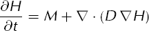
with diffusivity coefficient

(Reference Hindmarsh, Payne, Hooke and HutterHindmarsh and Payne, 1996; Reference Saito and Abe-OuchiSaito and Abe-Ouchi, 2005). The thermomechanically coupled formula combines Equations (1), (5) and (6). It is correct for arbitrary flow laws F(T, σ). This scalar quantity D, the diffusivity coefficient, is known numerically at every mass conservation time-step because it is the scalar factor involved in computing the flux Q. The identification Q = –D∇H is the ice flow analogue of Fourier’s law for heat, although the expression  where
where  is the vertically averaged horizontal velocity, also holds. As diffusion equations, (1) and (13) are simultaneously highly non-linear and highly degenerate. (‘Degenerate’ applies because D → 0 at margins and divides, where H → 0 and |∇H| → 0, respectively.)
The maximum value of D anywhere on an ice sheet controls the largest stable time-step for explicit approximations of Equation (1) (Reference Hindmarsh, Payne, Hooke and HutterHindmarsh and Payne, 1996; Reference Hindmarsh, Straughan, Greve, Ehrentraut and WangHindmarsh, 2001). Indeed, in the thermomechanically coupled case using the explicit numerical scheme described in Appendix A, we observe the stability restriction

The maximum is taken over values of D computed at every horizontal grid location (xi, yj ) on the simulated ice sheet at the current time-step tl.
Restriction (25) is reliable enough to use in an adaptive time-stepping scheme if advection in the temperature equation is also well approximated; see the comments on numerical approximation of the advection below. Our observed restriction (25) is only slightly more restrictive than that in the isothermal case, where Reference Hindmarsh, Straughan, Greve, Ehrentraut and WangHindmarsh (2001) predicts a critical value of the righthand side of (25) of 1/(2n) = 1/6. When the time-step violates inequality (25) the resulting stability problems (wiggles) emerge at locations on the ice sheet where the function H n+2|∇H| n–1 is largest. This will generically occur away from divides and margins.
Implicit schemes for Equation (1) avoid stability restrictions such as (25), but fully coupled implicit schemes are significantly harder to implement. In any case, there is an additional restriction on thermomechanically coupled timestepping, described next.
Domination of the temperature problem by vertical advection
In simulating real ice sheets, rough surfaces sometimes produce large vertical velocities in columns of ice below the roughness. Similarly, sliding laws which allow an abrupt onset of sliding adjacent to frozen bed areas can produce unreasonably large vertical velocities (through incompressibility). These large velocities can produce a poor approximation of the advection part of the temperature problem if the numerical time-step is not restricted.
To explain why large vertical velocities appear, supposewe combine Equations (5) and (7), and suppose for completeness there is a possibly non-zero basal horizontal velocity field U b and a possibly non-flat bed z = b. (We now need to distinguish between the surface elevation z = h and the thickness H.) Then
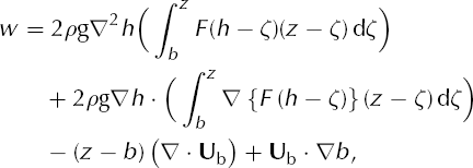
where F = F(T, σ) and ∇2 h = ∇·(∇h).One sees that the vertical velocity is affected by both the first and second derivatives of the surface h, by the divergence of U b and by the gradient of b. The integrals here are not the point;we are simply identifying dependencies on horizontal derivatives and thus on possible numerically induced inaccuracies.
Because the vertical velocity depends on the second derivative of the surface, it is more sensitive to surface roughness than are the horizontal velocity components (which depend only on the first derivatives of the surface elevation). In particular, a gridded (rectangular or triangular mesh) approximation of the surface elevation which is acceptable for computing horizontal velocity may be rough enough to cause unreasonable vertical velocities in some columns of ice. We observe, for instance, that digital elevation maps for Antarctica drive this effect in many locations when these maps are used as initial conditions for ice-sheet simulation.
The dependence of w upon the divergence of the basal horizontal velocity field has been observed before. For instance, EISMINT II experiment H, which involved pressuremelting temperature-activated basal sliding, has been criticized because it used basal velocities U b proportional to the effective shear stress and involved sudden transitions of the basal velocity as one moves from frozen base to melted base (Reference Fowler, Straughan, Greve, Ehrentraut and WangFowler, 2001). The resulting jump in U b produces unbounded vertical velocity within the ice in the continuum limit. Such discontinuities in basal velocity are presumably avoidable by using more complete physical models of the basal conditions.
Flow velocities are of importance here because they advect heat, and this advection must be numerically approximated. Numerical schemes for Equation (2) may have conditions on the length of the time-step in terms of the magnitude of the advection velocities. Upwinded schemes of any finite order require some version of the CFL condition (Reference Morton and MayersMorton and Mayers, 2005) for stability.
For example, we use a first-order upwind for temperature Equation (2); see Equation (A2) in Appendix A. This method sacrifices accuracy and it produces some artificial diffusivity but it is essentially as stable as possible (Reference Morton and MayersMorton and Mayers, 2005). For our scheme a precise form of the CFL condition for pure advection is the inequality

See Appendix B and Equation (B3) in particular. Here the numerators of the terms within parentheses are the gridded values of the components of velocity. The maximum is over the whole 3-D gridded region of ice at the time tl . Condition (27) is combined with condition (25) in our adaptive timestepping scheme, and the shorter of the two time-steps is used.
We observe in practice that condition (27) is more likely to be activated by large vertical velocities than horizontal velocities. Of course, vertical speeds in an ice sheet are typically lower in absolute terms than horizontal speeds, but the vertical mesh is always much finer. As described above, numerically computed vertical velocities can be of surprisingly large magnitude because of surface roughness and/or large gradients in the basal velocity field.
Payne and Dongelmans (1997) introduced a scheme with unequally spaced five-point upwinding which maintains stability with higher-order local truncation error.We believe this scheme, which is subject to some unstated CFL condition, is used in several current ice-sheet models. Such a scheme is definitely worthwhile if it can be shown that the global approximation error – the actual error – is reduced. The exact solutions of this paper are well suited to demonstrating such improved performance.
The strain-heating term: emergence of spokes
A standard finite-difference convergence analysis (Appendix B) of our scheme for Equation (2) reveals that if condition (27) holds for each time-step then the growth of the numerical error is controlled by two quantities. One quantity is the smoothness of the continuum solution to Equation (2), as reflected in the local truncation error of the scheme (Reference Morton and MayersMorton and Mayers, 2005). The other quantity, however, is the size of a derivative of the strain-heating term ∑. Recall that

Let El
be the maximum of the numerical temperature errors  over the entire spatial grid at time-step tl
. That is, consider the maximum of the difference between the computed approximate temperature Tijkl
and the exact temperature T(x, y, z, t) predicted by the continuum equations but evaluated at the gridpoint (xi
, yj
, zk
) at time tl; this is an instance of the definition of numerical error above. One can show (Appendix B) that
over the entire spatial grid at time-step tl
. That is, consider the maximum of the difference between the computed approximate temperature Tijkl
and the exact temperature T(x, y, z, t) predicted by the continuum equations but evaluated at the gridpoint (xi
, yj
, zk
) at time tl; this is an instance of the definition of numerical error above. One can show (Appendix B) that

where τl is the local truncation error at time tl . Note that τl depends on the size of higher partial derivatives of the exact solution to the temperature equation, that is, it depends on the smoothness of the continuum solution.
By inequality (29) the local truncation error can, at worst, cause arithmetic growth in the actual error El . By contrast, in estimate (29) the error El multiplies ∂Σ/∂T. The worst-case error can therefore grow exponentially (geometrically) if ∂Σ/∂T is large. The quantity ∂Σ/∂T acts like an interest rate for growth of error. A refined form of inequality (29) is inequality (B7), which shows that the exponential growth can be greatest at the locations where ∂Σ/∂T is maximum.
Consider the spokes which appear in EISMINT II experiment F, and are illustrated in Results above. Note that the EISMINT II experiment F continuum set-up has perfect angular symmetry. The exact solution of this initial/boundary value problem, which is unknown, also has this angular symmetry. Thus the magnitude of the spokes, as measured by the deviation from a given temperature value as one follows a curve of fixed z and r in a circle within the ice around the z axis, is a lower bound for the numerical temperature error. (In this literal sense, the spokes unequivocally are a numerical error.)
Figure 18 shows that ∂Σ/∂T has strong maxima along the warm spokes in EISMINT II experiment F. (In this figure, large values of ∂Σ/∂T for points where the thickness is less than 1000m are set to zero. We assert that these values are corrupted by margin mis-approximation, but that the slow flow very close to the margin (e.g. within 20 km of the margin) is unable to feed back to affect the surface slopes and near-basal strain rates at the upstream locations of the onset of spokes. Better numerical schemes for approximation of the fields near the margin may remove this issue (Reference Saito, Abe-Ouchi and BlatterSaito and others, 2007).)
Basal values of ∂∑/∂T (10–12s–1) from EISMINT experiment F, from the same computation which provided Figure 17. To give clear detail, only one-quarter of the computational region is shown.

Thus the spokes emerge under a version of the well-known thermocoupling feedback mechanism, with warmer spokes locally drawing down the surface and steepening the gradient nearby, thus increasing the strain heating upstream of the warm spokes, and generally accelerating flow to produce more strain heating, and so on. This describes ‘thermal runaway’, which is also observed in fluid systems other than ice (Reference Fowler, Straughan, Greve, Ehrentraut and WangFowler, 2001). The spokes themselves are errors, however, because the continuum problem and its unknown (exact) solution have angular symmetry. Thus the quantity which is ‘running away’ in this analysis is the size of the numbers  the numerical temperature errors.
The analysis here usefully predicts that spokes emerge in locations of peak values of the diagnostically computable quantity ∂Σ/∂T. On the other hand, the derivative of Σ with respect to T, using the second form of Σ in Equation (28), is:
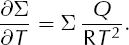
This quantity is always positive. From Equation (30) it follows that if a realistic Arrhenius-type term in the flow law is used with the Reference Paterson and BuddPaterson and Budd (1982) law as the representative case, then as the temperature rises from cold to within 10 K of the melting point the quantity ∂Σ/∂T will jump up discontinuously. The jump occurs at a temperature of 263.15 K in the Paterson–Budd relation, where Q changes from 6.0 to 13.9 (in units of 104 J mol–1): see Figure 19. Note Σ is a continuous function of temperature but ∂Σ/∂T is not in the Paterson-Budd case. The Hooke (1981) flow law, which has been demonstrated to produce spokes for experiment F in practice (Reference Payne and BaldwinPayne and Baldwin, 2000), apparently behaves in an even worse manner because the value of ∂Σ/∂T near melting is even larger, although there is no actual jump. This seems to cause even stronger error growth in the immediate vicinity of the margin.
Graphs A(T) for the Reference Paterson and BuddPaterson and Budd (1982) and Hooke (1981) flow laws, and of the cold and warm simple Arrhenius parts of the Paterson–Budd law extended to all temperatures. For the Paterson–Budd and Hooke laws the slope of A(T) jumps or changes rapidly as one approaches the melting temperature. Therefore ∂Σ/∂T jumps or changes rapidly; see Equation (28).

However, if the contribution of Σ to the temperature field as in Equation (2) is non-physically ‘smeared’ then the spokes go away. In particular, suppose we smooth the strain-heating term Σ in horizontal directions, at each temperature time-step, by replacing gridded values Σijk,l with an average of horizontally neighboring values. An example of the result for the basal temperature map is shown in Figure 20; the spokes are gone. In this case, the smoothing was by a finite-support averaging kernel which was approximately Gaussian and had a standard deviation of about two grid spaces (25 km) and a maximum range of four grid spaces (50 km) on this 12.5 km grid. From runs on various grids we believe the smoothing is effective in eliminating the spokes if it has a range (standard deviation) of the order of 25 km for a 1 year time-step.

The average was globally energy-conserving for the ice, that is, all of the heat generated by strain heating (and no more heat) was put into the ice. The location of that heating was spread in the horizontal by a mechanism not explained by the missing horizontal conduction terms in the conservation-of-energy equation, however. Easy estimates of the thermal diffusivity of ice show that our ad hoc smoothing is significantly greater than would be the effect of reintroducing horizontal conduction of heat through the ice or bed. (Neither of these reintroductions was numerically tested, however.) An interesting possibility is that the inclusion of longitudinal stresses into the coupled system would spread the strain heating itself in the horizontal (Reference HindmarshHindmarsh, 2006) and provide a physical mechanism which smears the spokes.
The ‘thermal runaway’ of the numerical temperature errors is rather slow in that it takes at least thousands of model years to become significant. It can only occur if the conditions causing the runaway remain in place for a significant time and apply over significant spatial extent. In particular, EISMINT II experiment F results show spokes in its flat base and smoothly varying accumulation conditions but they take more than 10 kyr to stabilize after the geometry is roughly in place. It is therefore likely that in conditions of significantly varying bed elevation, or of varying surface temperature and accumulation boundary conditions, the necessary coherence for thermomechanically coupled runaway of error does not occur. Thus the spokes phenomenon might be minimally influential for the simulation of real ice sheets.
The ‘thermal runaway’ of the error, though it may grow exponentially in some cases, has a maximal exponential rate if the geometry is fixed. In fact, one can turn inequality (29) into a proof of convergence of our numerical scheme for temperature under the assumption of fixed geometry and also stringent smoothness assumptions about the velocity fields (Reference Bueler and BrownBueler and Brown, 2006). This proof yields a maximum exponential rate based on the largest value of ∂Σ/∂T as described above.
We see no strong reason to believe that some version of the spokes will not appear when numerical 3-D thermomechanically coupled Stokes simulations are applied to circumstances similiar to EISMINT II experiment F. This is because the temperature equation keeps its same strain-heating term, and thus an analysis of the numerical error in the temperature equation will reveal the same possibility (at least) of ‘thermal runaway’ of the error. Indeed it appears that in at least one higher-order stress balance scheme there are still spokes for the EISMINT II experiment F boundary values (Reference Saito, Abe-Ouchi and BlatterSaito and others, 2006).
Discussion
The above analysis of the spokes in EISMINT II experiment F, which identifies them mathematically as numerical errors, is correct but it is also impoverished scientifically. The spokes are not merely telling us that there is some divergence of the numerical solution from the exact (and angularly symmetric) solution. Indeed, there is pattern to the numerical error, and the pattern comes from a mechanism in the thermomechanically coupled SIA which allows the ice flow to concentrate into spokes (Reference Payne and DongelmansPayne and Dongelmans, 1997). We would not want to claim that the spokes are solely a numerical artifact (Reference Saito, Abe-Ouchi and BlatterSaito and others, 2006) even though our mathematical analysis clearly identifies them as numerical errors. We now attempt to include both of these complementary interpretations of the spokes in the same discussion.
First note that, based on the verification performed in this paper, we can exclude the possibility that the spokes arose because the numerical scheme does not consistently approximate all the terms and all the coupling mechanisms in the continuum thermomechanically coupled SIA.
We have not observed any numerical evidence which suggests an unequivocal ill-posedness of the time-dependent problem. That is, we have never observed the effect that the numerical scheme is unable to maintain stability by choosing appropriately small time-steps. This would be the symptom if any numerical scheme were applied to the ill-posed backward heat equation ∂u/∂t = —∂2u/∂x 2, for instance. In such a case, the continuum dynamical system has the property that the rate of exponential explosion of modes of various spatial frequencies is an unbounded increasing function of the frequency. Numerically, all wiggles blow up and the more ‘wiggly’ they are the faster they blow up. Shortening the time-step would never help in this kind of problem.
On the other hand, the kind of ill-posedness claimed by Reference HindmarshHindmarsh (2004, Reference Hindmarsh2006), in particular, would be more subtle. Itwould correspond merely to non-decay of the rate of exponential growth of the modes as a function of the spatial frequency. We have not observed this phenomenon either, however. In particular, Figure 17 shows spokes with smooth contours. This must be because the highest-frequency components of the temperature variation actually decay slightly (i.e. some smoothing occurs). Note, however, that the spokes which appear when we use the Hooke (1981) flow law (not shown, but see similar results in Reference Payne and BaldwinPayne and Baldwin, 2000), do not have much smoothness. This could be evidence for the Reference HindmarshHindmarsh (2004) interpretation in the (non-standard) Hooke flow-law version of EISMINT II experiment F.
We believe that the specific time-dependent continuum dynamical system in question has an unstable equilibrium point. In particular, we believe that as the continuum solution evolves from the prescribed zero-ice initial condition, any added perturbation from perfect symmetry becomes a path which diverges from the intended path of ice sheets with perfect symmetry. Perturbations will, of course, inevitably happen with numerical errors, including rounding errors. But the unstable equilibrium is a property of the continuum dynamical system itself.
We propose that by tuning the central surface temperature from T min = 243 K (experiment A) to T min = 223 K (experiment F) the angularly symmetric equilibrium solution undergoes a bifurcation (Reference Guckenheimer and HolmesGuckenheimer and Holmes, 1983) from stable to unstable. The spokes we see represent a new stable equilibrium of a slightly perturbed continuum problem, which is significantly far away from the unstable angularly symmetric equilibrium of the unperturbed problem. Furthermore, it seems that the new stable equilibrium is relatively dependent on the details of the numerical discretization. Thus, one sees different forms for the spokes coming from different numerical schemes (Reference PaynePayne and others, 2000; Reference Saito, Abe-Ouchi and BlatterSaito and others, 2006; this paper).
Note that, if desired, one could approximate the angularly symmetric equilibrium by computing on a r, z cylindrical coordinate grid and thereby enforcing symmetry. We suspect that the instability is occurring in directions (in the relevant function space) which are orthogonal to the angularly symmetric states; compare the form of the most unstable mode in Reference HindmarshHindmarsh (2006). In other words, if we restrict ourselves to the angularly symmetric subspace then we expect there to be a stable equilibrium.
It is possible that a change to a more complete continuum model will eliminate the spokes problem by making the equilibrium stable. The addition of higher-order stresses by the Reference BlatterBlatter (1995) shallow approximation, however, seems not to eliminate the spokes (Reference Saito, Abe-Ouchi and BlatterSaito and others, 2006). On the other hand, Reference HindmarshHindmarsh (2006) performs a stability analysis which suggests that use of the Reference BlatterBlatter (1995) approximation should dampen the spokes instability.
We certainly believe that the form of the spokes, and even the existence of spoked stable equilibria, is sensitive to the source and boundary functions of the problem. We expect that the equilibrium solution is sensitive to the spatial distribution of the surface accumulation rate. Similarly, the equilibrium solution is a sensitive function of the surface temperature and of the shape of the bed. We therefore expect that the solution of the equilibrium continuum problem is very sensitive to the equilibrium climate. It might even be a discontinuous function of such an equilibrium climate. If the spokes represent the steady state that arises as the surface temperature parameter Tmin passes a bifurcation point, then the solution of the problem is certainly a discontinuous function of the climate.
We do not believe that the time-dependent problem is meaningfully ill-posed. But it seems likely to us that the equilibrium thermomechanically coupled problem is ill-posed in the sense that it depends discontinuously on the climate inputs to the ice-sheet model. It is an interesting question whether this situation applies to any continuum model of ice sheets which is sufficiently complete.
Conclusion
We have described the first non-trivial exact solutions of the thermomechanically coupled SIA. These exact solutions come with the caveat that a compensatory heat source is used in their construction. In these exact solutions, the temperature field at depth is not physical. We believe, however, that the glaciology community can substantially replace intercomparison with verification using exact solutions as a test method for numerical models of thermomechanically-coupled ice sheets based on the SIA.
The numerical scheme used by our group shows clear evidence of convergence under grid refinement when approximating these exact solutions.
Our numerical scheme also exhibits spokes, however, when approximating the unknown continuum solution to the EISMINT II experiment F boundary value problem (Reference PaynePayne and others, 2000). We assert that the spokes are literally a numerical error relative to the exact solution (which has angular symmetry). On the other hand, the spokes grow to a finite size through a physically significant mechanism (e.g. the mechanism discussed by Reference Payne and DongelmansPayne and Dongelmans, 1997). We show that a numerical solution can diverge exponentially from the exact solution at a rate which depends on the size of the derivative of the strain-heating term with respect to temperature. The equilibrium solution of EISMINT II experiment F is unstable, so this actually occurs.
The resulting spokes suggest that the function (map) from the climate data used in the model, in particular the accumulation and surface temperature data, to the solution of the equilibrium thermomechanically coupled SIA, is probably discontinuous.
Acknowledgements
We thank the NASA Cryospheric Sciences Program for support from grant No. NAG5-11371. The Arctic Region Supercomputing Center (ARSC), Fairbanks, Alaska, provided many hours of supercomputer time, and D. Bahls at ARSC, in particular, helped port our code to the big machines. D. Covey worked on early versions of our codes. Conversations and correspondence with F. Saito, M. Hagdorn, O. Lawlor and M. Truffer were invaluable. Finally, comments by referees A. Payne and C. Schoof significantly improved the paper and were much appreciated. In particular, our assessment of the ‘spokes’ in the Discussion was strongly influenced by Schoof’s insightful comments.
Appendix A: Numerical Scheme
The numerical scheme used to produce the results on verification and on EISMINT II experiment F is described here.
Note that the notation used here does not completely conform to Table 1. We assume, for the purposes of notational simplicity in this Appendix only, that there is only one horizontal coordinate x. A space–time gridpoint is denoted (xi, zk, tl ). We suppose that the ice sheet is, at all times, contained within a box (x, z) ∈ [–L max, L max] × [0, H max] and that Δ x = 2L max/N, Δ∑ = H max/N z. Gridded values of quantities independent of z are denoted here as Hij , etc., while quantities dependent on z are denoted Tikl , etc.
Equation (1) is approximated by

(In fact, Q = (Qx , Qy ) is a vector, but we are suppressing the y coordinate.) This is an explicit scheme because the right side contains only time tl values.
The temperature Equation (2) is approximated by an up-winded semi-implicit scheme. Let  and let Up
 The scheme is
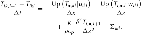
Both the upwinding and the semi-implicitness are chosen so that relatively long time-steps can be computed stably, but the time-step is still constrained by condition (27). Using boundary conditions (15) and (16), Equation (A2) can be rearranged to be a rapidly solvable tridiagonal system for the unknowns {T i,•,l+1} in the ith column of ice.
Note that boundary condition (15) is approximated by applying the value of the surface temperature to the highest gridpoint within the ice (at the given horizontal grid location). That is, boundary condition (15) is applied at the moving surface up to an error of order O(Δz). The Reference JenssenJenssen (1977) change of coordinates is not used.
To complete the above finite-difference equations we need to approximate u,w,Qx and Σ at time-step tl . We will both suppress the time index l and revert to two horizontal coordinates x and y. The surface gradient ΔH = ∂H/∂x, ∂H/∂y) is computed on a staggered grid by the Reference MahaffyMahaffy (1976) scheme:
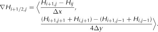
A similar formula computes ∇Hi,j+1/2. Using Equation (5) we compute the horizontal velocity on the staggered grid by integrating a scalar function in the vertical:

The integral is computed numerically by the trapezoid rule. Note  at ζ = zq
; see constitutive relation (4) for F(T , σ). Note that
at ζ = zq
; see constitutive relation (4) for F(T , σ). Note that 
 where Hi+1/2,j = (Hi+1,j + Hij)/2. Note also that the value Ti+1/2,j,k
is computed by averaging horizontal non-staggered grid neighbors. We find ui,j+1/2,k
and vi,j+1/2,k
by similar formulae to (A4).
where Hi+1/2,j = (Hi+1,j + Hij)/2. Note also that the value Ti+1/2,j,k
is computed by averaging horizontal non-staggered grid neighbors. We find ui,j+1/2,k
and vi,j+1/2,k
by similar formulae to (A4).
To compute  we vertically integrate the staggered grid values of u, computed from Equation (A4), by the trapezoid rule. To compute u
ikl for the first upwinded term in Equation (A2), we average horizontal staggered grid neighbors. To compute wikl
for the second upwinded term in Equation (A2), we use Equation (A4) and compute (∂u/∂x)ikl ≈ (ui+1/2,kl – ui–1/2,kl)/Δx and then integrate the result vertically by the trapezoid rule; see Equation (7). Finally, note that Σ = 2(ρcp)—1
F(T, σ)σ2 is first computed on the staggered grid by the Mahaffy choices for ∇H| and H in σ = ρg(H – z) |∇H|. These are then averaged onto the regular grid.
we vertically integrate the staggered grid values of u, computed from Equation (A4), by the trapezoid rule. To compute u
ikl for the first upwinded term in Equation (A2), we average horizontal staggered grid neighbors. To compute wikl
for the second upwinded term in Equation (A2), we use Equation (A4) and compute (∂u/∂x)ikl ≈ (ui+1/2,kl – ui–1/2,kl)/Δx and then integrate the result vertically by the trapezoid rule; see Equation (7). Finally, note that Σ = 2(ρcp)—1
F(T, σ)σ2 is first computed on the staggered grid by the Mahaffy choices for ∇H| and H in σ = ρg(H – z) |∇H|. These are then averaged onto the regular grid.
Appendix B: A Finite-Difference Error Analysis
Here we analyze the error in the finite-difference scheme (A2) which applies to the temperature Equation (2). This analysis of error is standard for finite-difference approximations of many PDEs (Reference Morton and MayersMorton and Mayers, 2005), but no similar analysis is known to the authors for the shallow ice flow conservation-of-energy equation. The most important assumptions made here are that the components of the velocity field are assumed to be fixed functions of space and time (independent of the temperature) and also that the geometry of the ice sheet is fixed. This analysis nonetheless provides enough information to build a reliable adaptive time-stepping scheme for the temperature equation in the fully coupled system. It also reveals a significant point of numerical error growth.
We analyze the numerical scheme in three spatial dimensions, that is, we add a second horizontal dimension to Equation (A2). In particular, the upwinded approximation to the advection term v ∂T/∂y is added. We suppose Equation (2) applies on some bounded region Ω which is fixed in time. We enclose Ω in a rectangular computational domain. We set a rectangular grid on that computational domain with spacing Δx, Δy, Δz. We denote the gridpoints by (x i, y, Zk). The interval of time is divided in an unequally spaced manner, but we use Δt for the current time-step in the analysis.
Let uijkl = u(xi, yj, Zk, tl ), etc. Let Tijkl be our numerical approximation of the temperature at a gridpoint. The gridded value of the exact solution is denoted T(xi, yj, Zk, tl ).
The local truncation error τijkl is defined to be the non-zero result of applying the finite-difference scheme to the exact solution T(x, y, z, t) (Reference Morton and MayersMorton and Mayers, 2005). It plays a supporting role in the analysis of the global approximation error (the actual numerical error). The local truncation error of our scheme decays to zero at rate O(Δt, Δx, Δy, Δz) as the grid is refined. Including the Taylor expansions and all cases of upwinding, it has the more detailed form of
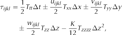
where the partial derivatives of T are evaluated somewhere in the neighborhood of (xi, yj, zk, tl ) and where K = k/(ρcp). We see that the finite-difference scheme is consistent (Reference Morton and MayersMorton and Mayers, 2005), that is, the local truncation error tends to zero as the grid is refined, assuming the exact solution is smooth enough. (This is the minimal situation in which we may proceed.)
Let eijkl = Tijki – T(xi, yj, zk, tl) be the (signed) numerical error at a gridpoint. Since Tijkl solves scheme (A2) exactly, and by the definition of the local truncation error,
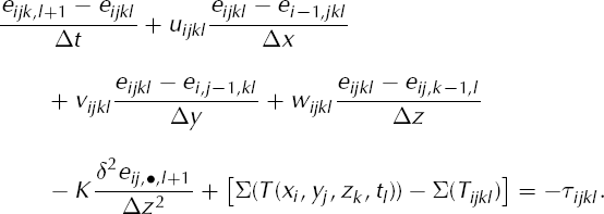
Equation (B2) and also (B3) below apply as stated only in the upwinding case of all positive components of velocity.
We are interested in the evolution of error so we solve for the error at gridpoint (x i, y j, zk ) at time t l+1:
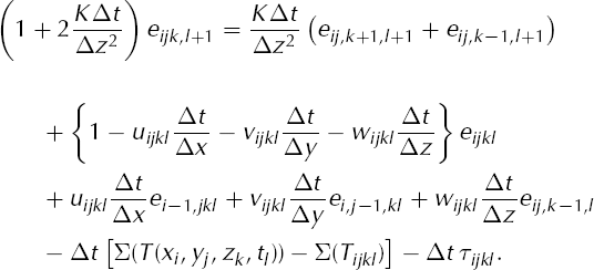
We now assume that the quantity in braces in Equation (B3) is non-negative in all upwinding cases, which is precisely the CFL condition (27). This assumption, which limits our time-step and generates part of the adaptive time-stepping scheme, allows us to proceed with a version of the standard maximum principle argument for a finite-difference scheme (Reference Morton and MayersMorton and Mayers, 2005, especially section 2.15). As is standard in such arguments, our plan is to use as a stability condition the assumption that all coefficients of errors are non-negative in Equation (B3).
Let El = maxi,j,k |eijkl and τl = maxi,j,k |τijkl|. Our goal is to know how much El can grow in one time-step. Equation (B3), considering all upwinding cases, and condition (27) together imply

The size of the |Σ(T(xi , yj , zk , tl )) – Σ(Tijkl )| term is very important, and we must make another assumption. It amounts to knowing that the derivative of Σ with respect to the temperature T is finite. This assumption is fully justified in the case of existing flow laws, but the size of this derivative, and of the coefficient L which appears next, is of importance in connection with the spokes; see Analysis.
We assume there exists a bounded non-negative function L(x, y, z, t) ≥ 0 such that

Note that the strain-heating term Σ actually depends on coordinates x, y, z and t as well as temperature T through its dependence on the thickness and surface slope of the ice sheet. In particular, if the partial derivative ∂Σ/∂T exists and is bounded, and if we define
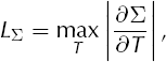
then we may take L = L Σ to make inequality (B5) true. The result is the inequality:
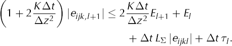
Inequality (B7) gives inequality (29) by considering the worst case location on the grid at time tl+1 , that is, at i, j, k such that |eijk,l +1| = El +1.
Regarding inequalities of the form of (B7) and/or (29), note that if

for some abstract sequence {αl}, given A > 0 and particular values B0, B1,..., then

Thus, coefficient A in (B8) controls exponential growth of {αl}, while the effect of large values of can only contribute linearly (arithmetically) to {αl }.
In the text we have exploited inequality (29) to substantially explain the spokes as numerical errors. In Reference Bueler and BrownBueler and Brown (2006) we also use inequality (B7) to build a convergence theorem for the finite-difference scheme under additional (admittedly stringent) smoothness assumptions.



