


1. Introduction
The Atlantic Meridional Overturning Circulation (AMOC) is a key process within the climate system, responsible for regulating the large-scale redistribution of heat, salinity and nutrient fluxes from low to high latitudes. The AMOC is driven by a combination of wind forcing in the subtropical gyres and buoyancy fluxes originating from surface cooling and brine rejection at high latitudes (Buckley & Marshall Reference Buckley and Marshall2016). In the subpolar North Atlantic, dense cold water forms through intense winter cooling, sinking to depth and returning southward along isopycnals. The upper branches of the AMOC typically carry warm, saline water northward, completing the loop. However, disentangling the relative contributions of wind-driven Ekman transports and density-driven convection to the overall overturning remains an area of active debate and dispute (Klocker et al. Reference Klocker, Munday, Gayen, Roquet and LaCasce2023). Specifically, to isolate solely the density-driven component, we present a reduced model, which is not intended to represent the full physical reality but rather to capture the buoyancy-driven component of the circulation in a simplified geometry. Therefore, the expression ‘AMOC in a box’ is used in a strictly idealised thermohaline sense, following previous minimal overturning models (Quon & Ghil Reference Quon and Ghil1992; Thual & Mcwilliams Reference Thual and Mcwilliams1992; Soons, Grafke & Dijkstra Reference Soons, Grafke and Dijkstra2025). The model is therefore not intended to represent the full wind- and buoyancy-driven ocean circulation.
As a very simplified model system for large-scale ocean circulation, horizontal convection (HC) has been suggested (Rossby Reference Rossby1965; Whitehead Reference Whitehead1995; Hughes & Griffiths Reference Hughes and Griffiths2008), where heat is supplied and removed through the upper surface. A significant number of studies have been dedicated to the characterisation of such a system, with the aim of analysing mean flow structure and heat transport scaling with the control parameters (Rossby Reference Rossby1965; Griffiths, Hughes & Gayen Reference Griffiths, Hughes and Gayen2013; Shishkina, Grossmann & Lohse Reference Shishkina, Grossmann and Lohse2016; Passaggia, Cohen & Scotti Reference Passaggia, Cohen and Scotti2024; Passaggia & Scotti Reference Passaggia and Scotti2024). Horizontal convection and/or a combination of HC and Rayleigh–Bénard convection is also used as a model system for subglacial lake (Couston, Nandaha & Favier Reference Couston, Nandaha and Favier2022; Rabaux et al. Reference Rabaux, Bu, Couston, Chillà and Salort2026). In order to mimic the AMOC dynamics, in the present study the combined effect of both temperature and salinity will be considered, namely double-diffusive horizontal convection (DDHC), whose defining property is a horizontal variability in both temperature and salinity. In double-diffusive convection (DDC) the fluid density depends on two scalar fields with, in general, different molecular diffusivities (Stern Reference Stern1960). Heat diffuses through water much faster than salt, giving rise to interesting and rich flow behaviour. Two types of DDC are of particular interest in the oceanographic context: salt-finger convection appears when warm, salty water overlies cooler and fresher water, as typical in the tropical oceans, whereas diffusive DDC forms when it is driven by an unstable temperature gradient, while the salinity gradient is stabilising (typically in the Arctic or Antarctic). This latter type of DDC can cause layer formation that controls vertical heat–salt exchange. A comprehensive overview of this topic can be found in Radko (Reference Radko2013) and Garaud (Reference Garaud2018). Both numerical (Schladow, Thomas & Koseff Reference Schladow, Thomas and Koseff1992; Simeonov & Stern Reference Simeonov and Stern2004; Radko Reference Radko2011; Yang et al. Reference Yang, Chen, Verzicco and Lohse2020) and experimental (Ruddick, Phillips & Turner Reference Ruddick, Phillips and Turner1999; Ruddick Reference Ruddick2003; Krishnamurti Reference Krishnamurti2006) studies have been performed with the goal of investigating horizontally spreading intrusions.
The effect of a background shear in a DDC configuration and its influence on the temperature and salt transport have been analysed by Radko et al. (Reference Radko, Ball, Colosi and Flanagan2015), Sichani et al. (Reference Sichani, Marchioli, Zonta and Soldati2020) and Yang et al. (Reference Yang, Verzicco, Lohse and Caulfield2022). Recent simulations of Li & Yang (Reference Li and Yang2022) demonstrate that even a very weak background shear can modify salt fingers into well-organised structure, markedly increasing the vertical salinity flux. Shear-affected DDC is particularly relevant in the present study because the double-diffusive dynamics develops within a persistent large-scale circulation, which naturally introduces velocity shear that interacts with the formation, growth and advection of double-diffusive structures.
The majority of the above cited studies has focused on a configuration in presence of vertical and horizontal gradients of temperature and salinity, including a uniform gradient and heated sidewall. The effect of imposed temperature and salinity gradients at the top boundary i.e. DDHC, has been less investigated. Whitehead (Reference Whitehead2021) carried out two-dimensional simulations in a rectangular domain with aspect ratio ( $\varGamma =W/H=8$
), imposing linear temperature and salinity distributions along the upper boundary. The salinity Rayleigh number was held fixed (
$\varGamma =W/H=8$
), imposing linear temperature and salinity distributions along the upper boundary. The salinity Rayleigh number was held fixed ( $\textit{Ra}_S=\mathcal{O}(10^5)$
) while the temperature Rayleigh number was varied, yielding a rich variety of flow patterns, including salty blobs and stripe-like structures. In the present work we focus on a slightly different forcing configuration and parameter range, and complement the phenomenological characterisation using global response parameters. Li & Yang (Reference Li and Yang2021) investigated, through three-dimensional numerical simulations, the flow-field features due to a smoothened step profile on the top wall for both salinity and temperature. That study, however, considers only the case where the buoyancy originated from temperature and salinity compensates. Their results extend the range of conditions under which thermohaline intrusions arise, demonstrating that they not only develop along horizontal density gradients but may also originate via vertical propagation between adjacent layers, scalar gradients at the bottom boundary and horizontal fluxes in overlying and underlying fluid layers.
$\textit{Ra}_S=\mathcal{O}(10^5)$
) while the temperature Rayleigh number was varied, yielding a rich variety of flow patterns, including salty blobs and stripe-like structures. In the present work we focus on a slightly different forcing configuration and parameter range, and complement the phenomenological characterisation using global response parameters. Li & Yang (Reference Li and Yang2021) investigated, through three-dimensional numerical simulations, the flow-field features due to a smoothened step profile on the top wall for both salinity and temperature. That study, however, considers only the case where the buoyancy originated from temperature and salinity compensates. Their results extend the range of conditions under which thermohaline intrusions arise, demonstrating that they not only develop along horizontal density gradients but may also originate via vertical propagation between adjacent layers, scalar gradients at the bottom boundary and horizontal fluxes in overlying and underlying fluid layers.
In this investigation, we present a series of numerical simulations aimed at extending the work of Li & Yang (Reference Li and Yang2021) across a broad range of density ratios. We identify four distinct regimes, each characterised by unique flow structures, and quantify their effects on global transport parameters. The paper is organised as follows: In § 2 we present the numerical set-up, the governing equations and the explored parameter space. Section 3 is split into two parts. In § 3.1 we discuss the global transport properties, while § 3.2 analyses the resulting flow-field structures. Finally, § 4 summarises the key findings and outlines possible future directions.
2. The ‘AMOC in a box’ system: geometry and underlying equations
The computational domain is sketched in figure 1. The upper wall is split into three parts: two side regions with fixed temperature and salinity, while the central part is assumed to be adiabatic with respect to both of them (zero flux). The left lateral region is warm and more salty $(T_+,\;S_+)$
, while the right counterpart is cold and less salty
$(T_+,\;S_+)$
, while the right counterpart is cold and less salty $(T_-,\;S_-)$
(see figure 1). We refer to the first as the equatorial plate and the second as the polar plate. Such a configuration has been inspired by several studies of HC (Shishkina & Wagner Reference Shishkina and Wagner2016; Shishkina Reference Shishkina2017), but here the focus is on DDHC.
$(T_-,\;S_-)$
(see figure 1). We refer to the first as the equatorial plate and the second as the polar plate. Such a configuration has been inspired by several studies of HC (Shishkina & Wagner Reference Shishkina and Wagner2016; Shishkina Reference Shishkina2017), but here the focus is on DDHC.
Sketch of the set-up with boundary conditions of the upper plate. In red the hot and more salty $(T_+,S_+)$
plate and in blue the cool and less salty
$(T_+,S_+)$
plate and in blue the cool and less salty $(T_-,S_-)$
plate, both of extension H in lateral direction.
$(T_-,S_-)$
plate, both of extension H in lateral direction.

To ensure a smooth transition between the isothermal and adiabatic horizontal walls, a Robin-type boundary condition
 \begin{equation} \chi (x)(T_{y=0}-T_{+,-}) + (1-\chi (x))\frac {\partial T}{\partial y}\Big |_{(y=0)}=0, \end{equation}
 \begin{equation} \chi (x)(S_{y=0}-S_{+,-}) + (1-\chi (x))\frac {\partial S}{\partial y}\Big |_{(y=0)}=0, \end{equation}
has been implemented. Depending on the $\chi$
value both Dirichlet and Neumann boundary conditions can be achieved. Indeed,
$\chi$
value both Dirichlet and Neumann boundary conditions can be achieved. Indeed, $\chi =1$
allows us to simulate Dirichlet boundary conditions, while
$\chi =1$
allows us to simulate Dirichlet boundary conditions, while $\chi =0$
corresponds to Neumann ones. Accordingly, the transition between the isothermal and adiabatic parts has been obtained by imposing a hyperbolic tangent variation of
$\chi =0$
corresponds to Neumann ones. Accordingly, the transition between the isothermal and adiabatic parts has been obtained by imposing a hyperbolic tangent variation of $\chi (x)$
between 1 and 0. The hyperbolic–tangent profile parameters were chosen so that the transition region spans
$\chi (x)$
between 1 and 0. The hyperbolic–tangent profile parameters were chosen so that the transition region spans $5\,\%$
of the isothermal plate length. This choice of parameters localises the transition zone while avoiding extreme sharpening. Even with an alternative boundary-condition configuration, our results remain in good agreement with Li & Yang (Reference Li and Yang2021), so the boundary-condition configuration has only a minor influence on the results.
$5\,\%$
of the isothermal plate length. This choice of parameters localises the transition zone while avoiding extreme sharpening. Even with an alternative boundary-condition configuration, our results remain in good agreement with Li & Yang (Reference Li and Yang2021), so the boundary-condition configuration has only a minor influence on the results.
At the bottom and vertical walls, a zero flux is set for both salinity and temperature and a no-slip condition is imposed. We perform both two-dimensional (2-D) and three-dimensional (3-D) numerical simulations. In the latter cases, periodicity is assumed in spanwise direction. We solve the Navier–Stokes equations, employing the Oberbeck–Boussinesq approximation (thus ignoring the density anomaly of water around $4\,^{\circ }\mathrm{C}$
), which in dimensionless form, read
$4\,^{\circ }\mathrm{C}$
), which in dimensionless form, read
 \begin{equation} \boldsymbol{\nabla } \boldsymbol{\cdot }\boldsymbol{u} = 0, \end{equation}
 \begin{equation} \frac {\partial \boldsymbol{u}}{\partial t} + \boldsymbol{\nabla }\boldsymbol{\cdot }(\boldsymbol{u} \boldsymbol{u}) = -\boldsymbol{\nabla } p + \left ( T - \frac {S}{\varLambda } \right ) \boldsymbol{\hat {e}}_y + \sqrt {\frac {\textit{Pr}}{\textit{Ra}_T}}{\nabla} ^2 \boldsymbol{u}, \end{equation}
 \begin{equation} \frac {\partial T}{\partial t} + \boldsymbol{\nabla } \boldsymbol{\cdot }(\boldsymbol{u} T) = \sqrt {\frac {1}{{\textit{Ra}_T \textit{Pr}}}} \, {\nabla} ^2 T, \end{equation}
 \begin{equation} \frac {\partial S}{\partial t} + \boldsymbol{\nabla } \boldsymbol{\cdot }(\boldsymbol{u} S) = \sqrt {\frac {1}{{\textit{Ra}_S \textit{Sc} }}}\,{\nabla} ^2 S. \end{equation}
In (2.3)–(2.6) ${\boldsymbol{u}}({x},t)$
denotes the velocity field,
${\boldsymbol{u}}({x},t)$
denotes the velocity field, $T(\boldsymbol{x},t)$
and
$T(\boldsymbol{x},t)$
and $S(\boldsymbol{x},t)$
are the temperature and salinity, respectively,
$S(\boldsymbol{x},t)$
are the temperature and salinity, respectively, $p(\boldsymbol{x},t)$
is the pressure and
$p(\boldsymbol{x},t)$
is the pressure and $\boldsymbol{\hat {e}}_y$
is the unit vector in the vertical direction . To non-dimensionalise the problem, the height of box
$\boldsymbol{\hat {e}}_y$
is the unit vector in the vertical direction . To non-dimensionalise the problem, the height of box $H$
is assumed as reference length scale and
$H$
is assumed as reference length scale and $\Delta T=T_+- T_-$
and
$\Delta T=T_+- T_-$
and $\Delta S=S_+-S_-$
are the temperature and salinity reference values, with
$\Delta S=S_+-S_-$
are the temperature and salinity reference values, with $T_{\pm }, S_{\pm } = \pm 0.5$
. As reference velocity we take the free fall velocity
$T_{\pm }, S_{\pm } = \pm 0.5$
. As reference velocity we take the free fall velocity $U_T=\sqrt {g \alpha H\Delta T}$
,
$U_T=\sqrt {g \alpha H\Delta T}$
, $g$
being the gravitational acceleration and
$g$
being the gravitational acceleration and $\alpha$
the thermal expansion coefficient. The problem is fully defined by the following dimensionless numbers: the Prandtl number, Schmidt number and Rayleigh numbers for both temperature and salinity
$\alpha$
the thermal expansion coefficient. The problem is fully defined by the following dimensionless numbers: the Prandtl number, Schmidt number and Rayleigh numbers for both temperature and salinity
 \begin{equation} \textit{Pr} = \nu /\kappa _T, \quad \textit{Sc} = \nu /\kappa _S, \quad \textit{Ra}_T = \frac { g \alpha H^3 \Delta T}{\nu \kappa _T}, \quad \textit{Ra}_S = \frac { g \beta H^3 \Delta S}{\nu \kappa _S}, \end{equation}
with $\nu$
the kinematic viscosity,
$\nu$
the kinematic viscosity, $\beta$
the salinity expansion coefficient and
$\beta$
the salinity expansion coefficient and $\kappa _T$
and
$\kappa _T$
and $\kappa _S$
the thermal and salinity diffusivity, respectively. Based on the dimensionless groups, the density ratio
$\kappa _S$
the thermal and salinity diffusivity, respectively. Based on the dimensionless groups, the density ratio $\varLambda$
is defined
$\varLambda$
is defined
 \begin{equation} \varLambda = \frac {\textit{Ra}_{\textit{TSc}}}{\textit{Ra}_S \textit{Pr}} = \frac {\alpha \Delta T}{\beta \Delta S}, \end{equation}
which quantifies the relative strength of buoyancy forces arising from temperature differences to those arising from salinity differences. From an oceanographic perspective, with the focus on AMOC, the inverse $\varLambda ^{-1}$
of the density ratio can be regarded as a proxy for the amount of freshwater introduced into the upper Arctic Ocean by melting glaciers. Lots of meltwater implies a large salinity difference
$\varLambda ^{-1}$
of the density ratio can be regarded as a proxy for the amount of freshwater introduced into the upper Arctic Ocean by melting glaciers. Lots of meltwater implies a large salinity difference $\Delta S$
and thus a small
$\Delta S$
and thus a small $\varLambda$
or large
$\varLambda$
or large $\varLambda ^{-1}$
. The ratio of the thermal and saline diffusivities can also be quantified by the Lewis number,
$\varLambda ^{-1}$
. The ratio of the thermal and saline diffusivities can also be quantified by the Lewis number, $\textit{Le} = \kappa _T / \kappa _S = \textit{Sc} / \textit{Pr}$
.
$\textit{Le} = \kappa _T / \kappa _S = \textit{Sc} / \textit{Pr}$
.
In the present investigation, fixed values of both the Prandtl and Schmidt numbers have been assumed, namely $\textit{Pr}=7$
and
$\textit{Pr}=7$
and $\textit{Sc}=21$
(and thus
$\textit{Sc}=21$
(and thus $\textit{Le}=3$
). Although
$\textit{Le}=3$
). Although $\textit{Sc}=21$
is far below the typical oceanic value of
$\textit{Sc}=21$
is far below the typical oceanic value of $\mathcal{O}(700)$
, lower Schmidt numbers are frequently employed in numerical investigations of DDC, e.g. Paparella & Von Hardenberg (Reference Paparella and Von Hardenberg2012) and Li & Yang (Reference Li and Yang2021), for computational ease. With the present value of the Schmidt number we have reproduced the effect of a reduced salinity diffusivity compared with that of temperature while still making it possible to adequately resolve the flow scales. Such a choice allowed us to investigate the effect of the density ratio. The complete list of simulations is presented in tables 1 and 2. Furthermore, by using
$\mathcal{O}(700)$
, lower Schmidt numbers are frequently employed in numerical investigations of DDC, e.g. Paparella & Von Hardenberg (Reference Paparella and Von Hardenberg2012) and Li & Yang (Reference Li and Yang2021), for computational ease. With the present value of the Schmidt number we have reproduced the effect of a reduced salinity diffusivity compared with that of temperature while still making it possible to adequately resolve the flow scales. Such a choice allowed us to investigate the effect of the density ratio. The complete list of simulations is presented in tables 1 and 2. Furthermore, by using $\textit{Sc}=21$
, we adopt a spatial resolution compatible with that used by Li & Yang (Reference Li and Yang2021). In particular, all simulations were performed with a resolution of
$\textit{Sc}=21$
, we adopt a spatial resolution compatible with that used by Li & Yang (Reference Li and Yang2021). In particular, all simulations were performed with a resolution of $288$
grid points in the wall–normal direction and
$288$
grid points in the wall–normal direction and $512$
points in the streamwise direction and, for the 3-D cases,
$512$
points in the streamwise direction and, for the 3-D cases, $128$
points in the spanwise direction. For the highest thermal Rayleigh number,
$128$
points in the spanwise direction. For the highest thermal Rayleigh number, $\textit{Ra}_T = 10^8$
, and for density ratios
$\textit{Ra}_T = 10^8$
, and for density ratios $\varLambda \leqslant 0.125$
, the resolution was doubled. To adequately resolve the boundary layers, a stretched grid was employed, see Chong et al. (Reference Chong, Yang, Wang, Verzicco and Lohse2020). Specifically, three values of
$\varLambda \leqslant 0.125$
, the resolution was doubled. To adequately resolve the boundary layers, a stretched grid was employed, see Chong et al. (Reference Chong, Yang, Wang, Verzicco and Lohse2020). Specifically, three values of $\textit{Ra}_T$
have been simulated, namely
$\textit{Ra}_T$
have been simulated, namely $10^6$
,
$10^6$
, $10^7$
and
$10^7$
and $10^8$
. Conversely, several values of
$10^8$
. Conversely, several values of $\textit{Ra}_S$
have been considered to cover a span of
$\textit{Ra}_S$
have been considered to cover a span of $\varLambda$
from
$\varLambda$
from $0.032$
up to
$0.032$
up to $32$
. The parameter space in an
$32$
. The parameter space in an $\varLambda -\textit{Ra}_T$
plane is shown figure 2(a). Numerical simulations have been performed by employing our in-house code which uses the fractional time step technique along with the finite-difference method (Van Der Poel et al. Reference Van Der Poel, Ostilla-Mónico, Donners and Verzicco2015) to solve the governing equations ((2.3)–(2.6)). The code has been widely applied to simulate convection flow, including DDC and wall-bounded turbulence; see Ostilla-Mónico et al. (Reference Ostilla-Mónico, Yang, Van Der Poel, Lohse and Verzicco2015) and Yang, Verzicco & Lohse (Reference Yang, Verzicco and Lohse2016). The complete documentation can be found in Howland (Reference Howland2022).
$\varLambda -\textit{Ra}_T$
plane is shown figure 2(a). Numerical simulations have been performed by employing our in-house code which uses the fractional time step technique along with the finite-difference method (Van Der Poel et al. Reference Van Der Poel, Ostilla-Mónico, Donners and Verzicco2015) to solve the governing equations ((2.3)–(2.6)). The code has been widely applied to simulate convection flow, including DDC and wall-bounded turbulence; see Ostilla-Mónico et al. (Reference Ostilla-Mónico, Yang, Van Der Poel, Lohse and Verzicco2015) and Yang, Verzicco & Lohse (Reference Yang, Verzicco and Lohse2016). The complete documentation can be found in Howland (Reference Howland2022).
(a) Phase diagram in the ( $\varLambda$
,
$\varLambda$
, $\textit{Ra}_T$
) parameter space. The circles indicate three-dimensional simulations, while the crosses represent two-dimensional simulations. (b) Reynolds numbers
$\textit{Ra}_T$
) parameter space. The circles indicate three-dimensional simulations, while the crosses represent two-dimensional simulations. (b) Reynolds numbers $\textit{Re}$
as function of the density ratio
$\textit{Re}$
as function of the density ratio $\varLambda$
for the different
$\varLambda$
for the different $\textit{Ra}_T$
, (c), (d) Nusselt numbers
$\textit{Ra}_T$
, (c), (d) Nusselt numbers $\textit{Nu}_T$
and
$\textit{Nu}_T$
and $\textit{Nu}_S$
, as functions of
$\textit{Nu}_S$
, as functions of $\varLambda$
, for different Rayleigh temperature numbers. The inset in (c) shows the temperature-driven HC scaling
$\varLambda$
, for different Rayleigh temperature numbers. The inset in (c) shows the temperature-driven HC scaling $\textit{Nu}_T \sim \textit{Ra}_T^{1/4}$
at
$\textit{Nu}_T \sim \textit{Ra}_T^{1/4}$
at $\varLambda = 32$
, while the inset in (d) shows the salinity-driven HC scaling
$\varLambda = 32$
, while the inset in (d) shows the salinity-driven HC scaling $\textit{Nu}_S \sim \textit{Ra}_S^{1/4}$
at low values of
$\textit{Nu}_S \sim \textit{Ra}_S^{1/4}$
at low values of $\varLambda$
, both consistent with the HC scalings relation of the Shishkina–Grossmann–Lohse (SGL) theory (Shishkina et al. Reference Shishkina, Grossmann and Lohse2016). The background colours highlight different regimes: blue represents temperature-driven HC, red oscillating regime, yellow layering and green salinity-driven HC.
$\varLambda$
, both consistent with the HC scalings relation of the Shishkina–Grossmann–Lohse (SGL) theory (Shishkina et al. Reference Shishkina, Grossmann and Lohse2016). The background colours highlight different regimes: blue represents temperature-driven HC, red oscillating regime, yellow layering and green salinity-driven HC.

Homogeneous initial conditions have been assumed for velocity, temperature and salinity. Initial temperature and salinity fields have been perturbed by superimposing random noise with an amplitude of $1\,\%$
. Furthermore, to investigate the dependence of the results on the initial conditions and the occurrence of hysteretic behaviour, specific analyses have been carried out. In more detail, at a given
$1\,\%$
. Furthermore, to investigate the dependence of the results on the initial conditions and the occurrence of hysteretic behaviour, specific analyses have been carried out. In more detail, at a given $\varLambda$
, the solution has been also computed starting from the available flow field determined with a lower
$\varLambda$
, the solution has been also computed starting from the available flow field determined with a lower $\varLambda$
value and increasing the ratio of the buoyancy forces. A similar procedure has been applied starting from the flow field computed with a larger
$\varLambda$
value and increasing the ratio of the buoyancy forces. A similar procedure has been applied starting from the flow field computed with a larger $\varLambda$
value, reducing the ratio of the buoyancy forces. It has been found that the solution is statistically independent of the initial conditions and hysteresis does not occur for the boundary conditions employed in this paper, in contrast to conceptually similar systems such as that in Soons et al. (Reference Soons, Grafke and Dijkstra2025).
$\varLambda$
value, reducing the ratio of the buoyancy forces. It has been found that the solution is statistically independent of the initial conditions and hysteresis does not occur for the boundary conditions employed in this paper, in contrast to conceptually similar systems such as that in Soons et al. (Reference Soons, Grafke and Dijkstra2025).
Temperature (a,b,c) and salinity (d,e, f) vertical profiles from the 2-D simulations, averaged in time and along the streamwise direction, in the warm and more salty (a,d), adiabatic (b,e) and cold and less salty (c, f) regions of the domain for various density ratios $\varLambda$
. Spatial averages are performed, excluding the transition zone. These profiles are representative of the four identified regimes. From 2-D simulation for
$\varLambda$
. Spatial averages are performed, excluding the transition zone. These profiles are representative of the four identified regimes. From 2-D simulation for $\textit{Ra}_T = 10^8$
.
$\textit{Ra}_T = 10^8$
.

3. Results
3.1. Transport properties
The background colours of figure 2 refer to four different regimes which have been identified in the present study and they will be described in detail in the following. The existence of these regimes was discerned through an analysis of the (temperature and salinity) Nusselt and Reynolds numbers as a function of $\varLambda$
. The temperature and salinity Nusselt numbers,
$\varLambda$
. The temperature and salinity Nusselt numbers, $\textit{Nu}_T$
and
$\textit{Nu}_T$
and $\textit{Nu}_S$
and the Reynolds number
$\textit{Nu}_S$
and the Reynolds number $\textit{Re}$
are defined as follows:
$\textit{Re}$
are defined as follows:
 \begin{equation} \textit{Nu}_T =\frac {\left \langle \partial T/\partial y\right \rangle _+ }{H/\Delta T}=-\frac {\left \langle \partial T/\partial y\right \rangle _- }{H/\Delta T}, \end{equation}
 \begin{equation} \textit{Nu}_S =\frac {\left \langle \partial S/\partial y\right \rangle _+ }{H/\Delta S}=-\frac {\left \langle \partial S/\partial y\right \rangle _- }{H/\Delta S}, \end{equation}
 \begin{equation} \textit{Re} = \frac {U_{\textit{rms}}H}{\nu }. \end{equation}
The symbol $\langle \boldsymbol{\cdot }\rangle _+$
represents the spatial mean on the warm and more salty plate, as well as over time. Similarly, the symbol
$\langle \boldsymbol{\cdot }\rangle _+$
represents the spatial mean on the warm and more salty plate, as well as over time. Similarly, the symbol $\langle \boldsymbol{\cdot }\rangle _-$
denotes the spatial mean on the cold and less salty plate, including the transition region, and over time.
$\langle \boldsymbol{\cdot }\rangle _-$
denotes the spatial mean on the cold and less salty plate, including the transition region, and over time.
As illustrated in figure 2, for large values of $\varLambda$
, as expected, the temperature-driven-dominated HC regime with a clockwise circulation is found. Both Nusselt and Reynolds numbers exhibit a tendency to a constant (
$\varLambda$
, as expected, the temperature-driven-dominated HC regime with a clockwise circulation is found. Both Nusselt and Reynolds numbers exhibit a tendency to a constant ( $\varLambda$
-independent) value, for a given
$\varLambda$
-independent) value, for a given $\textit{Ra}_T$
. Moreover, as expected, in this regime the temperature Nusselt is broadly consistent with the scaling
$\textit{Ra}_T$
. Moreover, as expected, in this regime the temperature Nusselt is broadly consistent with the scaling $\textit{Nu}_T \sim \textit{Ra}_T^{1/4}$
predicted by the SGL theory for HC (Shishkina et al. Reference Shishkina, Grossmann and Lohse2016), which is based on the Grossmann-Lohse theory for Rayleigh–Bénard convection (Grossmann & Lohse Reference Grossmann and Lohse2000; Lohse & Shishkina Reference Lohse and Shishkina2024), as visible in the inset of figure 2(c). It is worth noting, however, that the compensated curves retain a slight residual slope, indicating an effective exponent that is slightly smaller than
$\textit{Nu}_T \sim \textit{Ra}_T^{1/4}$
predicted by the SGL theory for HC (Shishkina et al. Reference Shishkina, Grossmann and Lohse2016), which is based on the Grossmann-Lohse theory for Rayleigh–Bénard convection (Grossmann & Lohse Reference Grossmann and Lohse2000; Lohse & Shishkina Reference Lohse and Shishkina2024), as visible in the inset of figure 2(c). It is worth noting, however, that the compensated curves retain a slight residual slope, indicating an effective exponent that is slightly smaller than $1/4$
for the present finite-
$1/4$
for the present finite- $\textit{Ra}_T$
dataset. For comparison, the
$\textit{Ra}_T$
dataset. For comparison, the $\textit{Nu}_T \sim \textit{Ra}_T^{1/5}$
scaling is also shown, valid for low Prandtl numbers (Shishkina et al. Reference Shishkina, Grossmann and Lohse2016). Furthermore, the results of the 3-D and 2-D simulations are in excellent agreement, showing that in this regime the flow field is essentially two–dimensional. The vertical salinity profiles averaged in time and along the streamwise direction within the equatorial (figure 3
d), purely adiabatic (figure 3
e) and polar (figure 3
f) regions of the domain, exhibit the characteristic behaviour of HC. As expected, in this temperature-dominated regime, salinity plays only a marginal role. The horizontal temperature gradient drives a flow toward the destabilising polar plate (see figure 3
f), where cold and less salty plumes form and penetrate the full depth, then return laterally along the bottom boundary.
$\textit{Nu}_T \sim \textit{Ra}_T^{1/5}$
scaling is also shown, valid for low Prandtl numbers (Shishkina et al. Reference Shishkina, Grossmann and Lohse2016). Furthermore, the results of the 3-D and 2-D simulations are in excellent agreement, showing that in this regime the flow field is essentially two–dimensional. The vertical salinity profiles averaged in time and along the streamwise direction within the equatorial (figure 3
d), purely adiabatic (figure 3
e) and polar (figure 3
f) regions of the domain, exhibit the characteristic behaviour of HC. As expected, in this temperature-dominated regime, salinity plays only a marginal role. The horizontal temperature gradient drives a flow toward the destabilising polar plate (see figure 3
f), where cold and less salty plumes form and penetrate the full depth, then return laterally along the bottom boundary.
As the density ratio $\varLambda$
decreases, we move into the convected finger regime, i.e. the red region of figure 2(d). The salinity transport
$\varLambda$
decreases, we move into the convected finger regime, i.e. the red region of figure 2(d). The salinity transport $(\textit{Nu}_S)$
increases, whereas the heat transport
$(\textit{Nu}_S)$
increases, whereas the heat transport $(\textit{Nu}_T)$
and the Reynolds number remain mostly unchanged. The
$(\textit{Nu}_T)$
and the Reynolds number remain mostly unchanged. The $\textit{Nu}_S$
enhancement arises from the formation of coherent, salinity-rich structures that are horizontally advected, increasing the convective transport. This is evident from the salinity profiles in figure 3: while they retain the shape of the HC, the cold and less salty plate regions exhibit an enhanced near-wall salinity (figure 3
e). This high concentration arises from the advection of coherent, salinity-rich structures onto the cold surface.
$\textit{Nu}_S$
enhancement arises from the formation of coherent, salinity-rich structures that are horizontally advected, increasing the convective transport. This is evident from the salinity profiles in figure 3: while they retain the shape of the HC, the cold and less salty plate regions exhibit an enhanced near-wall salinity (figure 3
e). This high concentration arises from the advection of coherent, salinity-rich structures onto the cold surface.
To rationalise this transition, we consider the ratio of relevant time scales, following the argument of Reiter & Shishkina (Reference Reiter and Shishkina2020). Specifically, convected fingers can develop when the growth time of salt-finger (SF) instabilities, $t_{\textit{SF}}$
, becomes shorter than the advection time scale
$t_{\textit{SF}}$
, becomes shorter than the advection time scale $t_{w\textit{ind}}$
associated with the temperature-driven HC. The advection time scale is defined as
$t_{w\textit{ind}}$
associated with the temperature-driven HC. The advection time scale is defined as $t_{w\textit{ind}} = L^2 / (\textit{Re}_L \nu )$
, where
$t_{w\textit{ind}} = L^2 / (\textit{Re}_L \nu )$
, where $\textit{Re}_L$
is the Reynolds number based on the horizontal length
$\textit{Re}_L$
is the Reynolds number based on the horizontal length $L$
. The time scale for the fastest-growing SF mode is given by the inverse of the growth rate
$L$
. The time scale for the fastest-growing SF mode is given by the inverse of the growth rate $\sigma _{\textit{max}}$
, derived from classical SF theory (Kunze Reference Kunze2003) (and shown as a plot in the supplementary material at https://doi.org/10.1017/jfm.2026.11442)
$\sigma _{\textit{max}}$
, derived from classical SF theory (Kunze Reference Kunze2003) (and shown as a plot in the supplementary material at https://doi.org/10.1017/jfm.2026.11442)
 \begin{align} \frac {{t}_{w\textit{ind}}}{{t}_{\textit{SF}}} = \frac {1}{2}\frac {\varGamma ^2}{\textit{Sc}\, \textit{Re}_L}\sqrt {\frac {\textit{Ra}_T \textit{Sc}}{\textit{Pr}}} \;\varPhi \left (\varLambda \right ) , \quad \text{with} \quad \varPhi \left (\varLambda \right ) =\sqrt { \frac {\textit{Sc}}{\textit{Pr} \varLambda }-1}\, \left (\sqrt { \varLambda }-\sqrt { \varLambda -1}\right )\! \end{align}
This relation indicates that unstable conditions are permitted only for density ratios in the range $1 \lt \varLambda \lt \textit{Sc}/\textit{Pr}$
. For a fixed
$1 \lt \varLambda \lt \textit{Sc}/\textit{Pr}$
. For a fixed $\textit{Ra}_T$
, the function
$\textit{Ra}_T$
, the function $\varPhi (\varLambda )$
increases as
$\varPhi (\varLambda )$
increases as $\varLambda$
decreases within this interval, so reducing
$\varLambda$
decreases within this interval, so reducing $\varLambda$
favours the condition
$\varLambda$
favours the condition $t_{\textit{SF}} \lt t_{w\textit{ind}}$
: SF instabilities can then grow before being swept away by the mean flow, and convected fingers appear. Conversely, for a fixed
$t_{\textit{SF}} \lt t_{w\textit{ind}}$
: SF instabilities can then grow before being swept away by the mean flow, and convected fingers appear. Conversely, for a fixed $\varLambda$
, the ratio
$\varLambda$
, the ratio $t_{w\textit{ind}}/t_{\textit{SF}}$
decreases as
$t_{w\textit{ind}}/t_{\textit{SF}}$
decreases as $\textit{Ra}_T$
decreases, because the increase of
$\textit{Ra}_T$
decreases, because the increase of $\textit{Re}_L$
with
$\textit{Re}_L$
with $\textit{Ra}_T$
is weaker than the
$\textit{Ra}_T$
is weaker than the $\sqrt {\textit{Ra}_T}$
factor in (3.4). If we take the value of
$\sqrt {\textit{Ra}_T}$
factor in (3.4). If we take the value of $t_{w\textit{ind}}/t_{\textit{SF}}$
obtained from (3.4) at
$t_{w\textit{ind}}/t_{\textit{SF}}$
obtained from (3.4) at $\textit{Ra}_T = 10^8$
and
$\textit{Ra}_T = 10^8$
and $\varLambda = 2.5$
as a threshold above which the instability can fully develop, then the same threshold is reached at lower values of
$\varLambda = 2.5$
as a threshold above which the instability can fully develop, then the same threshold is reached at lower values of $\varLambda$
when
$\varLambda$
when $\textit{Ra}_T$
is smaller. This behaviour is fully consistent with our direct numerical simulation (DNS) results: at high
$\textit{Ra}_T$
is smaller. This behaviour is fully consistent with our direct numerical simulation (DNS) results: at high $\textit{Ra}_T$
convected fingers appear over a broader portion of the salt-fingering interval.
$\textit{Ra}_T$
convected fingers appear over a broader portion of the salt-fingering interval.
A further $\varLambda$
reduction, i.e. an increase of
$\varLambda$
reduction, i.e. an increase of $\textit{Ra}_S$
, leads to the third regime (the layering regime), which is characterised by strong reductions of the
$\textit{Ra}_S$
, leads to the third regime (the layering regime), which is characterised by strong reductions of the $\textit{Nu}_S$
,
$\textit{Nu}_S$
, $\textit{Nu}_T$
and
$\textit{Nu}_T$
and $\textit{Re}$
values (see yellow region in figure 2). In this regime, in which
$\textit{Re}$
values (see yellow region in figure 2). In this regime, in which $\varLambda$
is of the order of unity, the buoyancy leading to circulation due to temperature is balanced by that due to salinity. The presence of layers strongly inhibits vertical transport, as observed in other work with different set-ups and flow conditions (Corcione, Grignaffini & Quintino Reference Corcione, Grignaffini and Quintino2015).
$\varLambda$
is of the order of unity, the buoyancy leading to circulation due to temperature is balanced by that due to salinity. The presence of layers strongly inhibits vertical transport, as observed in other work with different set-ups and flow conditions (Corcione, Grignaffini & Quintino Reference Corcione, Grignaffini and Quintino2015).
By further decreasing $\varLambda$
, the layers start to weaken and eventually disappear (salinity-driven HC regime). This fourth regime is again characterised by an horizontal convective flow, but, differently from the temperature-driven HC regime, it is governed by salinity and therefore the circulation is still horizontal, but with a reversed sign. This transition is smooth, and thus no sharply defined boundary can be identified; this is also evident from the gradual change in the flow structures, as the vertically migrating layers give way to the large-scale overturning patterns characteristic of salinity-driven HC. Figure 2(d) shows that
$\varLambda$
, the layers start to weaken and eventually disappear (salinity-driven HC regime). This fourth regime is again characterised by an horizontal convective flow, but, differently from the temperature-driven HC regime, it is governed by salinity and therefore the circulation is still horizontal, but with a reversed sign. This transition is smooth, and thus no sharply defined boundary can be identified; this is also evident from the gradual change in the flow structures, as the vertically migrating layers give way to the large-scale overturning patterns characteristic of salinity-driven HC. Figure 2(d) shows that $\textit{Nu}_S$
increases as
$\textit{Nu}_S$
increases as $\varLambda$
is reduced, and the inset suggests
$\varLambda$
is reduced, and the inset suggests $\textit{Nu}_S \sim \textit{Ra}_S^{1/4}$
, consistent with SGL scaling (Shishkina et al. Reference Shishkina, Grossmann and Lohse2016). The mean salinity profiles in figure 3(d–f) are also consistent with a salinity-driven HC structure. We therefore define the cross-over operationally from the compensated plots, using the onset of a flat compensated curve.
$\textit{Nu}_S \sim \textit{Ra}_S^{1/4}$
, consistent with SGL scaling (Shishkina et al. Reference Shishkina, Grossmann and Lohse2016). The mean salinity profiles in figure 3(d–f) are also consistent with a salinity-driven HC structure. We therefore define the cross-over operationally from the compensated plots, using the onset of a flat compensated curve.
Temporal history of salinity (top) and salinity convective flux in the lateral direction (bottom), both averaged across the purely adiabatic region of the domain, i.e. the region between the polar and equatorial plates: temperature-driven HC $\varLambda = 8$
(a), convected fingers
$\varLambda = 8$
(a), convected fingers $\varLambda = 1.5$
(b), layering
$\varLambda = 1.5$
(b), layering $\varLambda = 0.75$
(c) and salinity-driven HC
$\varLambda = 0.75$
(c) and salinity-driven HC $\varLambda = 0.06$
(d). In order to make the plot clearer we choose to report only part of the time history, dropping the first
$\varLambda = 0.06$
(d). In order to make the plot clearer we choose to report only part of the time history, dropping the first $42\,000$
time units. From 2-D simulation for
$42\,000$
time units. From 2-D simulation for $\textit{Ra}_T = 10^8$
.
$\textit{Ra}_T = 10^8$
.

3.2. Flow structures
Having discussed the global parameters and the time- and streamwise-averaged salinity profiles in § 3.1, we proceed examining the flow structures.
In the temperature driven HC regime, the imposed horizontal thermal gradient drives a clockwise circulation. The time histories of the salinity $ \langle S \rangle _a$
and its convective flux
$ \langle S \rangle _a$
and its convective flux $\langle u_xS \rangle _a$
, both averaged over the adiabatic region, show that there is a thin less salty layer near the top and a negative salinity convective flow flux near the wall (see figure 4
a).
$\langle u_xS \rangle _a$
, both averaged over the adiabatic region, show that there is a thin less salty layer near the top and a negative salinity convective flow flux near the wall (see figure 4
a).
The transition from the temperature-driven HC regime to one dominated by salt fingering is evident not only from the global parameters reported in figure 2 and from the time-scale argument discussed in § 3.1, but also from the temporal evolution of the absolute value of the salinity Nusselt number. As $\varLambda$
decreases, the time series
$\varLambda$
decreases, the time series $\textit{Nu}_S(t)$
(figure 5) display intermittent peaks associated with convective SF events. The quasi-periodicity of this oscillating SF can be interpreted in terms of the same time-scale balance introduced in § 3.1. In this regime, SFs repeatedly form, grow, detach and are advected horizontally by the large-scale circulation; one oscillation cycle corresponds to the time required for a finger to grow, detach and be swept away before a new one forms in its place. To illustrate this mechanism, we consider the case
$\textit{Nu}_S(t)$
(figure 5) display intermittent peaks associated with convective SF events. The quasi-periodicity of this oscillating SF can be interpreted in terms of the same time-scale balance introduced in § 3.1. In this regime, SFs repeatedly form, grow, detach and are advected horizontally by the large-scale circulation; one oscillation cycle corresponds to the time required for a finger to grow, detach and be swept away before a new one forms in its place. To illustrate this mechanism, we consider the case $\textit{Ra}_T = 10^8$
and
$\textit{Ra}_T = 10^8$
and $\varLambda = 2.5$
(figure 5
b). From the DNS signal we measure an oscillation period of the salinity flux
$\varLambda = 2.5$
(figure 5
b). From the DNS signal we measure an oscillation period of the salinity flux $t_{\textit{Nu}_S} \approx 400$
, as shown in figure 5(e). The advection time scale associated with the large-scale HC cell, estimated from the DNS Reynolds number and the aspect ratio, is
$t_{\textit{Nu}_S} \approx 400$
, as shown in figure 5(e). The advection time scale associated with the large-scale HC cell, estimated from the DNS Reynolds number and the aspect ratio, is $t_{w\textit{ind}} \approx 438$
, so that the two time scales are of the same order, with
$t_{w\textit{ind}} \approx 438$
, so that the two time scales are of the same order, with $t_{w\textit{ind}}/t_{\textit{Nu}_S} \approx 1.1 \gt 1$
. Higher-frequency overtones in the signal, with periods much shorter than
$t_{w\textit{ind}}/t_{\textit{Nu}_S} \approx 1.1 \gt 1$
. Higher-frequency overtones in the signal, with periods much shorter than $t_{w\textit{ind}}$
, are therefore expected to be unstable according to the SF stability criterion. Moreover, as
$t_{w\textit{ind}}$
, are therefore expected to be unstable according to the SF stability criterion. Moreover, as $\varLambda$
is reduced further, the peaks in the
$\varLambda$
is reduced further, the peaks in the $\textit{Nu}_S(t)$
time series become progressively more frequent (figure 5
c). The generation and propagation become almost continuous, precluding the identification of a single fundamental frequency.
$\textit{Nu}_S(t)$
time series become progressively more frequent (figure 5
c). The generation and propagation become almost continuous, precluding the identification of a single fundamental frequency.
Time series of the absolute salinity Nusselt number, $|\textit{Nu}_S|$
, on both plates for density ratios
$|\textit{Nu}_S|$
, on both plates for density ratios $\varLambda =4$
(a),
$\varLambda =4$
(a), $\varLambda =2.5$
(b) and
$\varLambda =2.5$
(b) and $\varLambda =1.5$
(c), at fixed
$\varLambda =1.5$
(c), at fixed $\textit{Ra}_T=10^8$
. As done in figure 4 for the purpose of graphic clarity, the times have been set to zero in the plot by dropping the first 42 000 time units.
$\textit{Ra}_T=10^8$
. As done in figure 4 for the purpose of graphic clarity, the times have been set to zero in the plot by dropping the first 42 000 time units.

Temporal and spatial averages $\textit{Re}_\tau$
vs
$\textit{Re}_\tau$
vs $\varLambda$
on the three plates: (a) equatorial plate on hot/more salty wall, (b) adiabatic plate centre on adiabatic wall and (c) polar plate on cold/less salty wall. The blue colour refers to
$\varLambda$
on the three plates: (a) equatorial plate on hot/more salty wall, (b) adiabatic plate centre on adiabatic wall and (c) polar plate on cold/less salty wall. The blue colour refers to $\textit{Ra}_T = 10^8$
, the red colour to
$\textit{Ra}_T = 10^8$
, the red colour to $\textit{Ra}_T = 10^7$
and the green colour
$\textit{Ra}_T = 10^7$
and the green colour $\textit{Ra}_T = 10^6$
. The circles represent 3-D simulations, while the crosses represent 2-D simulations.
$\textit{Ra}_T = 10^6$
. The circles represent 3-D simulations, while the crosses represent 2-D simulations.

The 2-D simulations show that extcolorblack convected SFs are periodically generated at the salt plate by the combined effects of horizontal shear-driven convection and salt fingering. These small SFs are subsequently advected in the streamwise direction toward the less salty side. A similar phenomenon has been observed by Whitehead (Reference Whitehead2021) in studying a DDHC set-up with a different distribution of the top wall temperature and salinity. The presence of these convected SFs causes the $\textit{Nu}_S (t )$
increase. Their periodical formation and propagation is responsible for the
$\textit{Nu}_S (t )$
increase. Their periodical formation and propagation is responsible for the $\textit{Nu}_S (t )$
oscillation. The SF migration has a direct influence onto the salinity profiles in the vertical direction, as shown in the § 3.1, and in addition on the friction Reynolds number
$\textit{Nu}_S (t )$
oscillation. The SF migration has a direct influence onto the salinity profiles in the vertical direction, as shown in the § 3.1, and in addition on the friction Reynolds number $\textit{Re}_\tau = u_\tau H/ (2 \nu )$
, where
$\textit{Re}_\tau = u_\tau H/ (2 \nu )$
, where $u_\tau = ( \langle \nu \partial _y u_x\rangle )^{1/2}$
.
$u_\tau = ( \langle \nu \partial _y u_x\rangle )^{1/2}$
.
Indeed, figure 6, reporting $\langle \textit{Re}_\tau \rangle$
versus
$\langle \textit{Re}_\tau \rangle$
versus $\varLambda$
, shows that in this regime the convected SFs generate an increase of the friction localised at the hot and more salty plate. Unlike the temperature-driven HC regime, in the second regime the 3-D simulations reveal the presence of SFs. In addition, 3-D simulations show that these fingers are unable to penetrate into the bulk region and to alter the circulation. However, they are convected by temperature-driven circulation and assume the form of a ‘streak-like’ pattern (figure 7
b). An analogous pattern was identified in the study of Li & Yang (Reference Li and Yang2022). The time periodic convected SF generation process is evidenced also by the time history of
$\varLambda$
, shows that in this regime the convected SFs generate an increase of the friction localised at the hot and more salty plate. Unlike the temperature-driven HC regime, in the second regime the 3-D simulations reveal the presence of SFs. In addition, 3-D simulations show that these fingers are unable to penetrate into the bulk region and to alter the circulation. However, they are convected by temperature-driven circulation and assume the form of a ‘streak-like’ pattern (figure 7
b). An analogous pattern was identified in the study of Li & Yang (Reference Li and Yang2022). The time periodic convected SF generation process is evidenced also by the time history of $\langle S \rangle _a$
(see figure 4
b). Indeed, figure 4 shows that positive salinity peaks begin to appear with a well-defined frequency. Such a phenomenon is more evident in the convective flux
$\langle S \rangle _a$
(see figure 4
b). Indeed, figure 4 shows that positive salinity peaks begin to appear with a well-defined frequency. Such a phenomenon is more evident in the convective flux $\langle u_xS \rangle _a$
history. In the convected fingers regime, figure 8 shows that, when decreasing
$\langle u_xS \rangle _a$
history. In the convected fingers regime, figure 8 shows that, when decreasing $\varLambda$
, SFs propagate progressively deeper. When the fingers penetrate sufficiently into the bulk region, eventually they produce the multi-layer structure illustrated by the 3-D salinity field in the figure 7(c).
$\varLambda$
, SFs propagate progressively deeper. When the fingers penetrate sufficiently into the bulk region, eventually they produce the multi-layer structure illustrated by the 3-D salinity field in the figure 7(c).
Instantaneous 3-D renderings of the salinity field at different density ratios $\varLambda$
:
$\varLambda$
: $\varLambda =8$
(a),
$\varLambda =8$
(a), $\varLambda =2$
(b),
$\varLambda =2$
(b), $\varLambda =0.75$
(c),
$\varLambda =0.75$
(c), $\varLambda =0.25$
(d); in all cases
$\varLambda =0.25$
(d); in all cases $\textit{Ra}_T=10^8$
.
$\textit{Ra}_T=10^8$
.

Instantaneous salinity fields in the spanwise wall-normal plane at $x = 0.5$
. Moving from left to right, the value of
$x = 0.5$
. Moving from left to right, the value of $\varLambda$
decreases, making the SFs become more and more prominent; in all cases
$\varLambda$
decreases, making the SFs become more and more prominent; in all cases $\textit{Ra}_T=10^8$
.
$\textit{Ra}_T=10^8$
.

In the layering regime, as $\varLambda$
decreases, the layers become more and more vigorous and begin to spread in the vertical direction. The process of layer migration, from the bottom toward the top walls, is clearly highlighted by the time history of both salinity
$\varLambda$
decreases, the layers become more and more vigorous and begin to spread in the vertical direction. The process of layer migration, from the bottom toward the top walls, is clearly highlighted by the time history of both salinity $\langle S\rangle _a$
and the salinity flux
$\langle S\rangle _a$
and the salinity flux $ \langle u_xS\rangle _a$
(figure 4
c). The
$ \langle u_xS\rangle _a$
(figure 4
c). The $\textit{Nu}_S$
time history, reported in figure 9, is characterised by the presence of a well-defined periodicity, with a low frequency,
$\textit{Nu}_S$
time history, reported in figure 9, is characterised by the presence of a well-defined periodicity, with a low frequency, $f_{\textit{Nu}_S}= 1/t_{\textit{Nu}_S}$
. This behaviour is related to the layer formation process, as shown in the snapshots of the streamwise velocity component at four different times, reported in figure 9. Moreover, figure 9 shows that the temporal evolution of
$f_{\textit{Nu}_S}= 1/t_{\textit{Nu}_S}$
. This behaviour is related to the layer formation process, as shown in the snapshots of the streamwise velocity component at four different times, reported in figure 9. Moreover, figure 9 shows that the temporal evolution of $\textit{Nu}_S$
occurs in opposite phase at the two plates. The quasi-periodic oscillations of
$\textit{Nu}_S$
occurs in opposite phase at the two plates. The quasi-periodic oscillations of $\textit{Nu}_S$
reflect the slow upward migration of the thermohaline layers. Across all
$\textit{Nu}_S$
reflect the slow upward migration of the thermohaline layers. Across all $\textit{Ra}_T$
, the relation
$\textit{Ra}_T$
, the relation $U_{\!s} \approx 2h/t_{\textit{Nu}_S}$
holds, indicating that each oscillation corresponds to an upward displacement of approximately two layer thicknesses, where
$U_{\!s} \approx 2h/t_{\textit{Nu}_S}$
holds, indicating that each oscillation corresponds to an upward displacement of approximately two layer thicknesses, where $U_{\!s}$
is the layer propagation speed and
$U_{\!s}$
is the layer propagation speed and $h$
the layer thickness. The spectral analysis of the
$h$
the layer thickness. The spectral analysis of the $\textit{Nu}_S(t)$
time series at
$\textit{Nu}_S(t)$
time series at $\varLambda = 0.75$
allowed us to find the fundamental period of the signal. Moreover, the same value of the fundamental period is found by analysing the time history of many pointwise quantities, such as the salinity, temperature and velocity components, at several points of the domain (results not shown here in the sake of conciseness).
$\varLambda = 0.75$
allowed us to find the fundamental period of the signal. Moreover, the same value of the fundamental period is found by analysing the time history of many pointwise quantities, such as the salinity, temperature and velocity components, at several points of the domain (results not shown here in the sake of conciseness).
Temporal history of $\textit{Nu}_S(t)$
for the right and left walls, in the layering regime
$\textit{Nu}_S(t)$
for the right and left walls, in the layering regime $\varLambda = 0.75$
,
$\varLambda = 0.75$
, $\textit{Ra}_T = 10^8$
. The panels show the streamwise velocity field at different times during the period. The times have been set to zero in the plot for clarity by dropping the first
$\textit{Ra}_T = 10^8$
. The panels show the streamwise velocity field at different times during the period. The times have been set to zero in the plot for clarity by dropping the first $42\,000$
time units.
$42\,000$
time units.

The difference between the first and last regimes in the plume generation and transport processes is clearly evidenced by figure 6. Indeed, figure 6 points out that, while over the cold/less salty plate higher $\langle \textit{Re}_{\tau } \rangle$
values are found at high
$\langle \textit{Re}_{\tau } \rangle$
values are found at high $\varLambda$
values (first regime), over the hot/more salty plate higher
$\varLambda$
values (first regime), over the hot/more salty plate higher $\langle \textit{Re}_{\tau } \rangle$
values occur at low
$\langle \textit{Re}_{\tau } \rangle$
values occur at low $\varLambda$
(last regime). This observation is consistent with the direction of the circulation. In the first regime, the plumes are generated below the cold/less salty plate, while in the last the opposite happens.
$\varLambda$
(last regime). This observation is consistent with the direction of the circulation. In the first regime, the plumes are generated below the cold/less salty plate, while in the last the opposite happens.
4. Conclusions and outlook
In this paper we have analysed the dynamics emerging in horizontal DDC phenomena as the density ratio varies. Four different regimes were found by observing both global response parameters and flow structures. The regime characterised by a ratio of the buoyancy forces $\varLambda$
close to unity (layering regime) presents a multi-layered structure that inhibits heat and salinity transport. Conversely, when
$\varLambda$
close to unity (layering regime) presents a multi-layered structure that inhibits heat and salinity transport. Conversely, when $\varLambda$
is slightly larger than one (oscillating convected SF regime), an increase in salinity transport is observed. For both high (temperature-driven HC regime) and low (salinity-driven HC regime)
$\varLambda$
is slightly larger than one (oscillating convected SF regime), an increase in salinity transport is observed. For both high (temperature-driven HC regime) and low (salinity-driven HC regime) $\varLambda$
values the scalings of standard HC are found and the SGL theory yields a unifying model for heat and salt transfer scaling.
$\varLambda$
values the scalings of standard HC are found and the SGL theory yields a unifying model for heat and salt transfer scaling.
The AMOC is characterised by a warmer northward flow at the top and a colder southward flow at the bottom. Therefore, its dynamics is similar to that of the temperature-driven HC regime. Although our model is highly idealised compared with the real AMOC, our results suggest that a reduction in the buoyancy ratio, caused, for instance, by an increase of glacial melting, could lead the system into a different regime, with significant consequences for heat and salt transport. However, the impact of different temperature and salinity boundary conditions on the system response remains to be assessed.
In future work we will explore mixed boundary conditions, i.e. combining fixed flux and fixed temperature at the top wall, with the aim of investigating the occurrence of hysteretic behaviour and the potential tipping points (Dijkstra & Molemaker Reference Dijkstra and Molemaker1997; Soons et al. Reference Soons, Grafke and Dijkstra2025) which were not found in the present configuration. Other interesting directions include more realistic boundary conditions, such as the effects of sea ice and solar radiation, as well as multi-ocean domain configurations, given the emerging evidence of Atlantic–Pacific coupling in driving the overturning circulation (Baker et al. Reference Baker, Bell, Jackson, Vallis, Watson and Wood2025). In addition, it would be natural to explore systematically the role of the Prandtl and Lewis numbers. This study is thus only a small step to better understand, from a fundamental and highly simplified point of view, the AMOC and other ocean circulations driven by DDC.
Supplementary material and movies
Supplementary material and movies are available at https://doi.org/10.1017/jfm.2026.11442.
Acknowledgements
We thank J. Salort and L. Couston for helpful discussions and the anonymous referees for helpful comments on the manuscript.
Funding
This work was financially supported by the European Union (ERC, MultiMelt, 101094492). Numerical resources were provided by the Gauss Centre for Supercomputing through project ID pr74sa on SuperMUC-NG, and by the EuroHPC Joint Undertaking for awarding the projects EHPC-REG-2022r03-208 and EHPC-REG2023R03-178 to access the EuroHPC supercomputer Discoverer, hosted by Sofia Tech Park (Bulgaria). We also acknowledge the Dutch national e-infrastructure with the support of SURF Cooperative.
Declaration of interests
The authors report no conflicts of interest.
Data availability statement
The data that support the findings of this study are available upon reasonable request.
Appendix
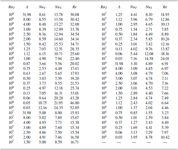
Summary of the control parameters and numerical results for the three-dimensional simulations.

Summary of the control parameters and numerical results for the two-dimensional simulations.


 Open access