


1. Introduction
Previously, research on aircraft icing was focused on the freezing of supercooled water droplets on the exterior of aircraft or on a sub-freezing engine surface. Since the mid-1990s, more than 200 engine power loss events were documented at altitudes of more than 7000 m where there is hardly any supercooled water content. In 2006, Mason et al. attributed these events to the ingestion of ice crystals generated by thunderstorms or convective storms (Mason, Strapp & Chow Reference Mason, Strapp and Chow2006). Under subfreezing conditions, ice crystals normally bounce off cold surfaces, and are relatively unproblematic; however, within an aeroengine compressor, the air temperature increases to above freezing. After ingestion into the compressor, ice crystals can melt, stick and accrete on the interior warm metal surfaces, leading eventually to flow blockage and subsequent engine power loss, stall and surge. Shedding of accumulated ice further damages engine components, promoting engine failure (Mason et al. Reference Mason, Strapp and Chow2006). Therefore, it has been recognised within the aeroengine industry that a deep understanding of the mechanisms and consequences of ice-crystal icing (ICI), including the accretion processes, is vital to ensure flight safety (Yamazaki, Jemcov & Sakaue Reference Yamazaki, Jemcov and Sakaue2021). Such an understanding is crucial for the implementation of safety protocols, the provision of pilot guidance and aircraft certification requirements and in underpinning the development of new technologies that can mitigate ice accretion and subsequent engine damage.
Experimental work performed in e.g. the NASA Glenn Research Center (Currie et al. Reference Currie, Struk, Tsao, Fuleki and Knezevici2012; Currie, Fuleki & Mahallati Reference Currie, Fuleki and Mahallati2014), RATFac Canada (Bucknell et al. Reference Bucknell, McGilvray, Gillespie, Parker, Forsyth, Ifti, Jones, Collier and Reed2019b) and Icing Wind Tunnel Braunschweig (Baumert et al. Reference Baumert, Bansmer, Trontin and Villedieu2018) has improved the understanding of the physical mechanisms of the ICI. It was shown that the accretion of mixed-phase water content was dependent on the ice fraction of the impinging water content, the ambient temperature and humidity conditions.
Numerous models have been adapted in order to account for ice-crystal accretion, including by Kintea et al. (Reference Kintea, Schremb, Roisman and Tropea2014), Kintea, Roisman & Tropea (Reference Kintea, Roisman and Tropea2016), Tsao, Struk & Oliver (Reference Tsao, Struk and Oliver2016), Bartkus, Struk & Tsao (Reference Bartkus, Struk and Tsao2018), Bartkus, Tsao & Struk (Reference Bartkus, Tsao and Struk2019), Villedieu, Trontin & Chauvin (Reference Villedieu, Trontin and Chauvin2014), Trontin & Villedieu (Reference Trontin and Villedieu2018), Bucknell et al. (Reference Bucknell, McGilvray, Gillespie, Jones and Collier2019a) and Ayan & Özgen (Reference Ayan and Özgen2018); these are often an extension of the model proposed by Messinger (Reference Messinger1953). More recent models that are based on the extended Messinger model (EMM) are by Ayan & Özgen (Reference Ayan and Özgen2018), who allowed for mixed-phase and glaciated conditions but only for sub-freezing temperatures, as well as Bucknell et al. (Reference Bucknell, McGilvray, Gillespie, Jones and Collier2019a), who adapted the EMM for above freezing temperatures. A summary of previous works on ICI can be found in table 1.
A selection of different formulations used for modelling ICI in engines. We introduce the following notation to refer to the substratum (substr.): FT (freezing temperature), C (coupling between the accretion and substratum), P (prescribed heat flux or temperature) and U (unspecified).

Bucknell et al. (Reference Bucknell, McGilvray, Gillespie, Jones and Collier2019a) developed a three-layer thermodynamic model for ice accretion, which accounts for warm surfaces and mixed-phase conditions. In the case of a warm substrate, the model is split into two regimes: (i) running wet conditions where there exists only a water film and all impinging ice is melted; (ii) if the water layer surface temperature reaches freezing, an ice layer forms over the water film and is in turn below a small surface-water film. However, the model is based on the assumption that all the impinging ice in the second regime accumulates into a pure solid ice layer. This is not a representation of the ice accretion physics observed by Malik et al. (Reference Malik, Köbschall, Bansmer, Tropea, Hussong and Villedieu2024), who showed that the accretion layer is a mixed-phase combination of water and ice. Therefore, this paper is to present a novel one-dimensional (1-D) model of ICI with a warm substrate and a mixed-phase icing layer.
At the melting point, the liquid water and ice have the same temperature but different enthalpies. This enthalpy difference is referred to as the latent heat of fusion. The enthalpy level of the mixture can be used to quantify the ice fraction. In addition, the interface between the pure water layer and the mixed-phase layer can be determined from the enthalpy distribution, which, as discussed by Crank (Reference Crank1984), simplifies the simulation of moving boundary problems. Further advances in numerical schemes for enthalpy such as the flag scheme developed by Bridge & Wetton (Reference Bridge and Wetton2007) ensure accuracy with reduced computation cost. Therefore, we study the enthalpy formulation of the problem. In addition, the formulation of the model used by Bucknell et al. (Reference Bucknell, McGilvray, Gillespie, Jones and Collier2019a) is also studied for comparison. The main differences between the two models are:
(i) The three-layer model of Bucknell et al. (Reference Bucknell, McGilvray, Gillespie, Jones and Collier2019a), outlined in § 2, serves as an extension to the EMM (Myers Reference Myers2001) for substrate temperatures above freezing. The model initially contains one water layer. When the water surface reaches freezing temperature, it transitions to a three-layer configuration, consisting of water, ice and water layers. The partially melted ice particles lead to surface accretion. In the presence of just one water layer, it is assumed that this ice immediately melts. When all three layers are present, the surface accretion contributes to both the ice layer and the top water layer. It is important to note that the quasi-steady model used in Bucknell et al. (Reference Bucknell, McGilvray, Gillespie, Jones and Collier2019a) ignores the contribution of the transient terms when solving heat transfer within accretion layers; in this work, we show that this effect may be significant under certain engine representative conditions.
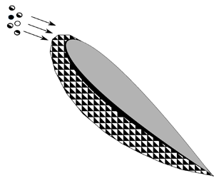
(ii) The new enthalpy model, developed in § 3, ultimately leads to a two-layer configuration consisting of a water phase and a mixed water/ice phase (mush), as illustrated in figure 1. This is a partial differential equation (PDE) with a single free boundary at the surface. Since the enthalpy is defined as the sum of sensible and latent heats, it is capable of capturing multiple layers, and phase changes, without the specification of interfacial equations. After freezing temperature is reached, the model effectively contains a lower water layer, and an upper mushy layer with mixed-phase properties of ice and water.
The governing equations are non-dimensionalised, showing that the icing problem is controlled by a substantial group of non-dimensional parameters, including the Péclet number  $Pe$, Stefan number $St$, melt ratio $Mr$, Biot number $Bi$, non-dimensional evaporative mass flux $\dot {m}_{ev}$, ratio of latent heats $L$ and the kinetic ratio $D$. In addition, we shall develop asymptotic approximations in the limit of $Pe \to 0$; these provide simple expressions for water and ice growth rates for both the three-layer and enthalpy models. The leading-order approximation is equivalent to the solution if the heat transfer within the accretion layers is assumed to be quasi-steady (the transient term in heat equations are ignored, which, in fact, is the assumption used by Bucknell et al. (Reference Bucknell, McGilvray, Gillespie, Jones and Collier2019a) to solve the temperature distribution within the accretion layers). The asymptotic approximations are compared with numerical simulations of the transient equations for both models. The difference between the accretion characteristics of both models are compared and discussed, and parametric studies are conducted to show the effects of non-dimensional parameters. Our analysis, including the asymptotic approximations, allows clear identification of the role of different parameters in the dynamics of the ICI problem. Prior works of the general ICI problem have not performed asymptotic analysis to this level of detail; as the complexity of the problem increases (to include, e.g. three-dimensional dynamics) the asymptotic growth laws developed in this work is useful for benchmarking and validation purposes.
Schematic of the accretion composition for incoming mass flux on a warm substrate as described by the enthalpy model in § 3. This consists of a thin water layer on the substrate, with a mixed-phase water/ice (mush) composition on top.

1.1. Outline of the paper
The transient, three-layer formulation of water–ice–water is derived in § 2. We develop our enthalpy model in § 3; this captures mixed-phase regions of water and ice. The key dimensional and non-dimensional parameters are given in § 4, in which the values used in our models are provided. Asymptotic solutions for small Péclet number are developed in § 5, for both phases of the three-layer model and for our enthalpy model. Comparisons with numerical solutions are presented in § 6. Section 7 summarises the key conclusions, and further discussion occurs in § 8.
2. Mathematical formulation of a three-layer model
Previously, ICI models which implemented the supercooled droplet model of Messinger (Reference Messinger1953) or the EMM (Myers Reference Myers2001) have assumed a substrate temperature that is below or equal to freezing temperature (Ayan & Özgen Reference Ayan and Özgen2018). In such models, ice is the first layer present on the solid surface. This incorrectly models the formation of ice within engines, in which the first layer must be water due to the presence of a warm substrate (Bucknell et al. Reference Bucknell, McGilvray, Gillespie, Yang, Jones and Collier2019c). The three-layer water–ice–water model, developed by Bucknell et al. (Reference Bucknell, McGilvray, Gillespie, Jones and Collier2019a), was designed as a further extension to the EMM, primarily to allow for substrate temperatures above freezing. In this section, we review this latter model; however, instead of assuming quasi-steady heat transfer we solve the transient equations using a fixed front method in which the interface between the water and ice layers is tracked and must be determined as part of the solution. The EMM is formulated in § 2.1, the modifications required to include a warm substrate are detailed in the water layer formulation of § 2.2 and the water–ice–water layer formulation of § 2.3. We non-dimensionalise the governing system in § 2.4, and discuss its connection with the enthalpy model of ICI, developed later in § 3.
2.1. A review of the extended Messinger model
We now introduce the dimensional formulation of the EMM, for which a typical solution is shown in figure 2. Solutions of this formulation will depend on the coordinates  $z$ and $t$, where $z$ is the spatial coordinate orthogonal to the lower substrate, and $t$ is time. We denote the thickness of the lower ice layer by $h_{ice}(t)$, and the thickness of the upper water layer by $h_{water}(t)$, both of which will be solved for as part of the solution. The total height of the domain is then given by $z = h_{ice}(t)+ h_{water}(t)$. The ice temperature, $T_{ice}(z,t)$, will then be solved for across $0 \leq z \leq h_{ice}(t)$, and the water temperature, $T_{water}(z,t)$, will be solved for across $h_{ice}(t) \leq z \leq h_{ice}(t) + h_{water}(t)$.
Form of icing captured in the original Messinger model, as depicted in Myers (Reference Myers2001).

The governing equations consist of mass conservation for the total growth of the system
 \begin{equation} \rho_{w}\frac{{\rm d}h_{water}}{{\rm d}t} + \rho_{i}\frac{{\rm d}h_{ice}}{{\rm d}t} = \dot{m}_{imp}-\dot{m}_{{ev,sub}}, \end{equation}
where  $\dot {m}_{imp}$ is the impinging mass flux which can be broken into water and ice contributions; this contribution crucially depends on the melt ratio, which is the ratio of liquid water content to total (ice + water) water content in the incoming ice particles (Currie et al. Reference Currie, Fuleki, Knezevici and MacLeod2013). Note that we assume the temperature of the incoming liquid water and ice content stays at the freezing temperature ( $T_{frz}=0\,^\circ {\rm C}$). We also have mass transfer via the evaporative/sublimative flux, $\dot {m}_{{ev,sub}}$; dependent on the surrounding conditions, this evaporative/sublimative flux can then model the gain or loss of mass (cf. Appendix B). Above, $\rho _w$ and $\rho _i$ correspond to the densities of water and ice, respectively. Typical values of these parameters are listed later in table 2.
Typical values of dimensional quantities under engine representative conditions, as used in the existing literature. Note that some estimates given in the references are more specified and single valued. Others are variable under variable engine or flow conditions.

The temperatures in the ice and water layers are given by 1-D heat equations
 $$\begin{gather} \rho_{i} c_{i} \frac{\partial T_{ice}}{\partial t} =k_{i}\frac{\partial^2 T_{ice}}{\partial z^2} \quad \text{for} \ 0 \leq z \leq h_{ice}(t), \end{gather}$$
 $$\begin{gather}\rho_{w} c_{w} \frac{\partial T_{water}}{\partial t} =k_{w}\frac{\partial^2 T_{water}}{\partial z^2} \quad \text{for} \ h_{ice}(t) \leq z \leq h_{ice}(t)+h_{water}(t), \end{gather}$$
where  $c_{w}, k_{w},c_{i},k_{i}$ denote the heat capacity and thermal conductivity of water and ice, and typical values can be found in table 2.
In the original model by Messinger (Reference Messinger1953) (and also discussed in the extended model by Myers (Reference Myers2001)), only supercooled water droplets are assumed, and the substrate, at  $z = 0$, is considered to be held at a temperature below the point of freezing. As a result, all incoming water is assumed to freeze, leading to the instantaneous formation of an ice layer with $T_{ice} < 0$ – this is the situation of rime ice. As it concerns (2.1a), only the growth of the ice layer needs to be considered ( $h_{water} = 0$), and we only need to consider the temperature profile in the ice given by (2.1b).
As noted by Myers (Reference Myers2001), in certain situations and under suitable flux conditions, the surface temperature of the ice layer, i.e.  $T_{ice}(h_{ice}(t), t)$, can reach the freezing temperature, thus allowing formation of a water layer on top; this leads to the setup known as glaze ice. In this case, we also need to consider the temperature of the water given by (2.1c), as well as an additional energy balance on the ice-water interface given by the Stefan condition
 \begin{equation} \rho_{i}L_{f} \frac{\mathrm{d}h_{ice}}{\mathrm{d}t}={-}k_{w} \frac{\partial T_{water}}{\partial z} + k_{i} \frac{\partial T_{ice}}{\partial z} \quad \text{at} \ z = h_{ice}(t), \end{equation}
where we have introduced the latent heat of fusion given by  $L_{f}$. Note that non-dimensionalising (2.1c) leads to the Péclet number
 \begin{equation} Pe = \frac{\rho_{w} c_{w} [H]^2}{k_{w}[t]}, \end{equation}
where  $[H]$ and $[t]$ correspond to typical length and temporal scales. Then $Pe$ governs the balance between advective and diffusive effects, and is often assumed to be small. When $Pe \ll 1$, the problem becomes quasi-steady as the time derivative components in each heat equation become subdominant. Indeed this assumption was used by a number of authors including Bucknell et al. (Reference Bucknell, McGilvray, Gillespie, Jones and Collier2019a) and Gallia et al. (Reference Gallia, Rausa, Martuffo and Guardone2023).
Finally, there are a number of assumptions that underpin the above model. These include: (i) lateral conduction is neglected; (ii) there is perfect thermal contact between the accretion and the substrate; (iii) the ice–water interfaces are at the freezing temperature; (iv) conduction within the substrate is not considered and the substrate temperature is prescribed.
The model developed by Bucknell et al. (Reference Bucknell, McGilvray, Gillespie, Jones and Collier2019a), denoted by the three-layer model, builds on the EMM discussed above, but considers two stages for the situation of a warm substrate and partially melted impinging water content. The original dimensional quasi-steady form of the model was presented in Bucknell et al. (Reference Bucknell, McGilvray, Gillespie, Jones and Collier2019a). Our goal in the next two subsections is to re-interpret the fully transient formulation of the model rigorously and to derive a non-dimensional form.
2.2. Stage 1 of Bucknell's model for ice-crystal icing (water only)
In stage 1, all the ice in the impinging water content melts, and leads to the formation of a water layer on the solid substrate. The formation of the initial water layer serves to trap more incoming particles, and thus leads to additional build-up of water. If the energy from melting is not balanced from other contributions, such as via convective and kinetic transport, this leads to a reduction in the water surface temperature. Then, if the temperature at the water surface drops to the freezing temperature, this then brings the model to stage 2, which permits the modelling of both an ice layer and a surface-water layer. These two stages are shown in figure 3.
Schematic of the two stages in the three-layer model of ICI as developed in Bucknell et al. (Reference Bucknell, McGilvray, Gillespie, Jones and Collier2019a). Initially, (a) in stage 1, there is only a water film; then in (b) stage 2, an water–ice–water layer is used.

We begin by considering the water-only state, as shown in figure 3(a). In this first stage, we are interested in the height and temperature of the water. Note that, in contrast to the EMM, the water layer,  $h_{water}(t)$, is now resting on the substrate. We seek to solve
 $$\begin{gather} \rho c_{w} \frac{\partial T_{water}}{\partial t} =k_{w}\frac{\partial^2 T_{water}}{\partial z^2} \quad \text{for} \ 0 \leq z \leq h_{water}(t), \end{gather}$$
 $$\begin{gather}\rho \frac{\mathrm{d}h_{water}}{\mathrm{d}t}= \dot{m}_{imp} - \dot{m}_{ev}(T_{water}) \quad \text{at} \ z=h_{water}(t). \end{gather}$$
The growth of the water layer is given by the continuity equation (2.3b). Our system starts from a clean substrate, and thus we have the following initial condition for the water layer:
 \begin{equation} h_{water}(0) = 0. \end{equation}
We then impose boundary conditions for the temperature
 $$\begin{gather} T_{water}=T_{subs} \quad \text{at} \ z=0, \end{gather}$$
 $$\begin{gather}-k_{w}\frac{\partial T_{water}}{\partial z} = \varPhi_{I}(T_{water}) \quad \text{at} \ z=h_{water}(t), \end{gather}$$
where the water adopts the positive substrate temperature,  $T_{subs}>0$, on the substrate, and there is a heat flux $\varPhi _{I}$ on the exposed water surface. The function $\varPhi _{I}$ can be broken down into components that are dependent on the surface temperature $T_{water}(h_{water}(t),t)$, such as evaporation, convection and sensible heat fluxes; it should also be considered as functions of components that are independent of $T_{surf}$, such as the melting/freezing and kinetic energies. For the sensible heat flux, we assume that impinging water and ice are at the freezing temperature, $T_{frz}$. Thus, following Bucknell et al. (Reference Bucknell, McGilvray, Gillespie, Jones and Collier2019a), we have the following makeup of the flux term:
 \begin{align} \varPhi_{I}(T_{water}) &= [\underbrace{\vphantom{\tfrac{1}{2}}h_{tc}(T_{water}-T_{rec})}_{convection}] + [\underbrace{\vphantom{\tfrac{1}{2}}L_{v}\dot{m}_{ev}(T_{water})}_{evaporation}] + [\underbrace{\vphantom{\tfrac{1}{2}}L_{f}\dot{m}_{{imp,i}}}_{{melt/freeze}}] \nonumber\\ &\quad +[\underbrace{\vphantom{\tfrac{1}{2}}c_{w}\dot{m}_{imp}(T_{water}-T_{frz})}_{sensible}] - [\underbrace{\tfrac{1}{2}\dot{m}_{imp}\bar{U}^2}_{kinetic}]. \end{align}
Here, we have introduced the recovery temperature  $T_{rec}$ and velocity of the incoming particles $\bar {U}$. We shall later provide typical parameter ranges of the contributions above in § 2.4. While complicated, the functional form of $\varPhi _{I}(T)$ in (2.4) is linear in $T$ for all terms with the exception of the evaporation, $\dot {m}_{ev}(T)$, which is a nonlinear function. Later, it will be further non-dimensionalised. A typical non-dimensional shape for $\varPhi _{I}$ is shown in figure 4. Note that at $T_{water}(h_{water}(t),t)=0$, we observe a jump to $\varPhi _{II}$ as the system enters stage two, described in § 2.3.


Under the appropriate conditions (i.e. an incoming flux of ice and water), the above system is evolved until the surface temperature reaches freezing, i.e.  $T_{water}(h_{water}(t^*),t^*)=T_{frz}=0\,^{\circ }{\rm C}$. Here, $t^*$ denotes the critical time at which point freezing occurs at the corresponding water thickness, $h_{water}^*=h_{water}(t^*)$. Dependent on initial and boundary conditions, such a finite-time freezing event may not occur; in this work, we focus on situations where it does.
2.3. Stage 2 of the three-layer model for ice-crystal icing
Once a freezing event occurs at a critical time,  $t = t^*$, and height, $h_{water} = h_{water}^*$, in the single-layer formulation of § 2.2, we proceed to the second stage in which three distinct water–ice–water layers are modelled. As is shown in figure 3(b), the domain is now bounded by $0 \leq z \leq h_{water}(t) + h_{ice}(t) + h_{surf}(t)$. This corresponds to internal water height $h_{water}$, middle ice layer $h_{ice}$, and top surface-water layer $h_{surf}$. We therefore introduce the following notation for the absolute heights:
 \begin{equation} \left.\begin{array}{@{}c@{}} z_{w}(t) \equiv h_{water}(t), \\ z_{wi}(t) \equiv h_{water}(t) + h_{ice}(t), \\ z_{top}(t) \equiv h_{water}(t) + h_{ice}(t) + h_{surf}(t), \end{array}\right\} \end{equation}
in addition to the corresponding domain for each layer
 \begin{equation} \left.\begin{array}{@{}c@{}} \varOmega_{b.\ water} \ \text{(bottom water region)} = \{z: z\in [0, z_{w}(t)]\}, \\ \varOmega_{ice} \ \text{(middle ice region)} = \{z: z\in [z_{w}(t), z_{wi}(t)]\}, \\ \varOmega_{t.\ water} \ \text{(top water region)} = \{z: z\in [z_{wi}(t), z_{top}(t)]\}. \end{array}\right\} \end{equation}
We also need to solve for the temperatures within each of the three different layers, which are given by  $T_{water}(z,t)$ for $z \in \varOmega _{b.\ water}$; $T_{ice}(z,t)$ for $z \in \varOmega _{ice}$; and $T_{surf}(z,t)$ for $z \in \varOmega _{t.\ water}$.
Only the temperatures of the internal water and ice layers will be solved for in this model. These are
 $$\begin{gather} \rho c_{w} \frac{\partial T_{water}}{\partial t} =k_{w}\frac{\partial^2 T_{water}}{\partial z^2} \quad \text{for} \ z \in \varOmega_{b.\ water}, \end{gather}$$
 $$\begin{gather}\rho c_{i} \frac{\partial T_{ice}}{\partial t} =k_{i}\frac{\partial^2 T_{ice}}{\partial z^2} \quad \text{for} \ z \in \varOmega_{ice}. \end{gather}$$
As noted in § 2.1, the above heat equations are typically solved under the quasi-steady assumption (cf. Myers (Reference Myers2001) for supercooled water and by Bucknell et al. (Reference Bucknell, McGilvray, Gillespie, Jones and Collier2019a) for ICI). Thus, the time-dependent left-hand sides are often neglected in implementations within the literature.
On the bottom substrate, we have
 \begin{equation} T_{water}(z,t)=T_{subs} \quad \text{at}\ z=0. \end{equation}
 In order to model the top water film, and in consideration of the fact that there is a complicated exchange of ice and water from the incoming flux, an additional assumption is made over the original Messinger model of § 2.1. Since the surface water film is typically very thin, (Bucknell et al. Reference Bucknell, McGilvray, Gillespie, Yang, Jones and Collier2019c, p. 5) assumes that the temperature gradient can be ignored and (since  $T_{surf}(z_{wi}(t),t)=0$), the top water film can be considered homogeneous in temperature
 \begin{equation} T_{surf}(z,t) \equiv 0 \quad \text{for} \ z \in \varOmega_{t.\ water}. \end{equation}
We also provide the interfacial boundary conditions for the internal water and ice layers, which by assumption from § 2.1 are all at the freezing temperature
 \begin{equation} T_{water}(z_{w}(t),t)=T_{ice}(z_{w}(t),t)=T_{ice}(z_{wi}(t),t) = 0. \end{equation}
The temperature gradient across the surface-water layer is related to the heat flux on the exposed surface, hence by (2.7d) the net heat flux is zero. Then on the exposed surface
 \begin{equation} \varPhi_{II}(\dot{m}_f) =0 \quad \text{at}\ z=z_{top}(t), \end{equation}
where the flux,  $\varPhi _{II}(\dot {m}_{f})$, takes a similar form to that of $\varPhi _{I}$ presented previously for the water-only case in (2.4)
 \begin{align} \varPhi_{II}(\dot{m}_{f})& = \underbrace{h_{tc}(T_{surf}-T_{rec})}_{convection} + \underbrace{L_{v}\dot{m}_{ev}(T_{surf})}_{evaporation}-\underbrace{L_{f}\dot{m}_{f}}_{{melting/freezing}}\nonumber\\ &\quad +\underbrace{\vphantom{\tfrac{1}{2}}c_{w}\dot{m}_{imp}(T_{surf}-T_{frz})}_{sensible} -\underbrace{\tfrac{1}{2}\dot{m}_{imp}\bar{U}^2}_{kinetic}, \end{align}
where, from (2.7d),  $T_{surf} = 0$, and as before $T_{frz}=0$ is the freezing temperature.
Studying (2.7g), we see that  $\varPhi _{II}$ has the same convection, evaporation, sensible and kinetic terms as the water-only case with $\varPhi _I$, but now the surface temperature $T_{surf}$ has replaced the former $T_{water}(h_{water}(t),t)$. Another difference is that the freezing/melting contributions on the right hand-side take a different form as we have entered stage 2, and we no longer require that all particles melt. The melting contribution ( $L_{f}\dot {m}_{{imp,i}}$) from $\varPhi _{I}$ (2.4) is then replaced with a freezing contribution, $-L_{f}\dot {m}_{f}$, in $\varPhi _{II}$.
In the end, (2.7f) and (2.7g) provide an equation which is solved for the mass flux between the ice and surface-water layer which is freezing, denoted by  $\dot {m}_{f}$.
For the internal water growth of  $h_{water}(t)$, a Stefan condition drives the water–ice interface, similar to the original EMM
 \begin{equation} \rho_{w}L_{f} \frac{\mathrm{d}h_{water}}{\mathrm{d}t}={-}k_{w} \frac{\partial T_{water}}{\partial z} + k_{i} \frac{\partial T_{ice}}{\partial z} \quad \text{at} \ z=z_{w}(t).\end{equation}
From (2.7e), the temperature within the ice layer should be invariant at the freezing temperature and the temperature gradient should be zero, hence  $T_{ice}=0$ and ${\partial T_{ice}}/{\partial z} = 0$. The ice layer, $h_{ice}(t)$, must consider the evolution of both interfaces, at $z=z_{w}(t)$ and $z=z_{wi}(t)$. It is modelled by
 \begin{equation} \rho_{i}\frac{{\rm d}h_{ice}}{{\rm d}t} ={-} \rho_{w}\frac{{\rm d}h_{water}}{{\rm d}t} +(\dot{m}_{{imp,i}}+ \dot{m}_{f}). \end{equation}
Above, the first term on the right-hand side is from the Stefan condition, as any growth from the internal water layer corresponds to melting from the ice layer. The second term on the right-hand side,  $\dot {m}_{imp,i}$, is from the impingement of penetrating ice particles. The last term on the right-hand side, $\dot {m}_{f}$, is the melting/freezing mass flux which is a solution of the boundary condition (2.7c).
The surface-water film,  $h_{surf}(t)$, grows according to
 \begin{equation} \rho \frac{\mathrm{d}h_{surf}}{\mathrm{d}t}= \dot{m}_{{imp,w}} - \dot{m}_{f} - \dot{m}_{ev}(T_{surf}) \quad \text{at} \ z=z_{top}(t), \end{equation}
where  $\dot {m}_{{imp,w}}$ is the liquid portion of the incoming mass, and $\dot {m}_{f}$ is the melting/freezing contribution between the surface-water layer and the ice layer, as solved above from (2.7c).
To close the system, we provide initial conditions for the heights of the different layers, which are given by
 \begin{equation} h_{water}(t^*) = h_{water}^*, \quad h_{ice}(t^*) = 0. \end{equation}
We note that Bucknell et al. (Reference Bucknell, McGilvray, Gillespie, Jones and Collier2019a) uses a quasi-steady assumption, in which time dependence is neglected in each of the heat equations for the water and ice. This includes (2.3a) for the water in stage 1, and (2.7a,b) for the lower water and middle ice layers, respectively, in stage 2. Time dependence only appeared in their model through the evolution equations for each interface. The model that we have presented in §§ 2.2 and 2.3 contains fully transient behaviour.
2.3.1. A remark on the instantaneous passage of ice to the ice layer
We mention one key remark with how the above governing equations are developed from Bucknell et al. (Reference Bucknell, McGilvray, Gillespie, Jones and Collier2019a). When considering the surface-water film and ice layer, the authors allow the ice contributions from incoming particles to (instantaneously) penetrate through the water layer, so that ice is added directly to the ice layer below. This behaviour is implemented via a split of the impinging mass flux,  $\dot {m}_{imp}$, into the water ( $\dot {m}_{imp,w}$) and ice ( $\dot {m}_{imp,i}$) contributions. Thus, water is added to the top water layer directly via a source term (cf. (2.7j)) while ice is added directly to the ice layer (cf. (2.7i)). Although unphysical, this modelling assumption has the advantage that the constituent makeup of the top-most layer (i.e. whether it is water, ice, or a mixture) does not have to be considered.
2.4. Non-dimensionalisation of the three-layer model
We begin by examining the different mass fluxes appearing in (2.7i) and (2.7j). We can split our impinging mass flux into water and ice contributions which is determined by the melt ratio,  $M_r$. Thus, we introduce this parameter to distinguish between water and ice impingement, setting
 \begin{equation} \dot{m}_{imp,w} = M_{r}\dot{m}_{imp} \quad \text{and} \quad \dot{m}_{imp,i} = (1-M_{r}) \dot{m}_{imp}. \end{equation}
We now scale our different mass flux by the total impingement, using the notation of hats to denote non-dimensional quantities
 \begin{equation} \left.\begin{array}{@{}c@{}} \hat{\dot{m}}_{imp,w} = \dfrac{ \dot{m}_{imp,w}}{\dot{m}_{imp}}=M_{r}, \quad \hat{\dot{m}}_{imp,i} = \dfrac{ \dot{m}_{imp,i}}{\dot{m}_{imp}}=1-M_{r}, \\[12pt] \hat{\dot{m}}_{f} = \dfrac{ \dot{m}_{f}}{\dot{m}_{imp}}, \quad \hat{\dot{m}}_{ev} = \dfrac{\dot{m}_{ev}}{\dot{m}_{imp}}. \end{array}\right\} \end{equation}
2.4.1. Stage 1 (water only)
We now non-dimensionalise the water-only system of (2.3). The following non-dimensional scalings are introduced for the spatial and temporal variables:
 \begin{equation} \left.\begin{array}{@{}c@{}} \hat{z}=\dfrac{z}{[H]}, \quad \hat{h}_{water}=\dfrac{{h_{water}}}{[H]}, \quad \hat{t}=\dfrac{t}{[t]}=\dfrac{\dot{m}_{imp} t}{\rho_{w} [H]},\\[12pt] \hat{T}_{water}=\dfrac{{T_{water}}}{T_{rec}}, \quad \hat{T}_{subs}=\dfrac{T_{subs}}{T_{rec}}. \end{array}\right\} \end{equation}
The time scale has been chosen to correspond to the rate at which mass enters the system via  $\dot {m}_{imp}$. Note that we relabel the temperature $\hat {T}_{water} \mapsto \hat {T}$ on the assumption that it is clear where the temperature is measured.
This yields the following non-dimensional governing equations:
 $$\begin{gather} Pe\frac{\partial {\hat{T}}}{\partial {\hat{t}}}=\frac{\partial^2 {\hat{T}}}{\partial {\hat{z}}^2}, \quad \text{for } \hat{z}\in\varOmega_{b.\ water}, \end{gather}$$
 $$\begin{gather}\frac{\mathrm{d}{\hat{h}_{water}}}{\mathrm{d}{\hat{t}}}= 1 - \hat{\dot{m}}_{ev}, \quad \text{at } \hat{z} = \hat{h}_{water}(\hat{t}). \end{gather}$$
The temperature conditions (2.7f) and (2.7c) at the solid substrate and free surface, respectively, satisfy
 $$\begin{gather} \hat{T} =\hat{T}_{subs}, \quad \text{at } \hat{z} = 0, \end{gather}$$
 $$\begin{gather}-\frac{\partial \hat{T}}{\partial \hat{z}} = \varPhi_{I}(\hat{T}(\hat{z}, \hat{t})), \quad \text{at } \hat{z} = \hat{h}_{water}(\hat{t}). \end{gather}$$
Above, and from (2.4) we have the flux,  $\varPhi _{I}$ defined as
 \begin{equation} \hat{\varPhi}_{I} \equiv {Bi}(\hat{T}-1) + {St}\,L \hat{\dot{m}}_{ev}(\hat{T}) +{St} (1-M_{r}) +Pe\,\hat{T}- {St}\,D. \end{equation}
We have also introduced the following non-dimensional parameters:
 \begin{equation} \left.\begin{array}{@{}c@{}} Pe = \dfrac{\dot{m}_{imp} c_{w} [H]}{k_{w}}, \quad {Bi}=\dfrac{h_{tc}[H]}{k_{w}}, \quad {St} = \dfrac{\dot{m}_{imp} L_{f}[H]}{k_{w} T_{rec}},\\[12pt] D=\dfrac{\bar{U}^2}{2L_{f}}, \quad L = \dfrac{L_{v}}{L_{f}}, \quad H = \dfrac{c_{i}}{c_{w}}, \end{array}\right\} \end{equation}
respectively corresponding to the Péclet number, Biot number, Stefan number, a ratio of kinetic to freezing energy and the ratio of latent heats. We will discuss typical parameter ranges in § 4. For the water height, a reasonable estimate is  $[H] \approx 10^{-4}$ m (Bucknell Reference Bucknell2018).
2.4.2. Stage 2 (three-layer configuration)
In addition to the above, we non-dimensionalise  $h_{ice}(t)$ and $h_{surf}(t)$ with respect to $[H]$, as well as temperature with respect to $T_{rec}$. This yields the additional non-dimensional quantities
 \begin{equation} \hat{h}_{ice}=\frac{{h_{ice}}}{[H]}, \quad \hat{h}_{surf}=\frac{{h_{water}}}{[H]}, \quad \hat{T}_{ice} = \frac{T_{ice}}{T_{rec}}. \end{equation}
 It should be noted that, in the three-layer model, the ice and top surface-water layer are always assumed to be at  $\hat {T}_{ice} \equiv 0$ and $\hat {T}_{surf} \equiv 0$. Therefore, only the temperature of the lower water layer must be solved
 \begin{equation} Pe_{w} \frac{\partial \hat{T}}{\partial \hat{t}} =\frac{\partial^2 \hat{T}}{\partial \hat{z}^2}, \quad \text{for} \ \hat{z} \in \varOmega_{b.\ water}, \end{equation}
with  $\hat {T} = \hat {T}_{water}$ above.
The layer growths are rewritten from (2.7h), (2.7i) and (2.7j) as
 $$\begin{gather} \frac{\mathrm{d}\hat{h}_{water}}{\mathrm{d}\hat{t}}= \frac{1}{St} \left(- \frac{\partial \hat{T}}{\partial \hat{z}} \right) \quad \text{at}\ \hat{z}=\hat{h}_{water}(\hat{t}), \end{gather}$$
 $$\begin{gather}\frac{{\rm d}\hat{h}_{ice}}{{\rm d}\hat{t}} = \frac{1}{R} \left[ -\frac{{\rm d}\hat{h}_{water}}{{\rm d}\hat{t}}+(1-M_{r})+ \hat{\dot{m}}_{f} \right], \end{gather}$$
 $$\begin{gather}\frac{\mathrm{d}\hat{h}_{surf}}{\mathrm{d}\hat{t}}= M_{r} - \hat{\dot{m}}_{f} - \hat{\dot{m}}_{ev}(\hat{T} = 0). \end{gather}$$
Again, since  $\hat {T}_{ice} \equiv 0$, the ice temperature disappears in the Stefan condition of (2.14b), and because $\hat {T}_{surf} \equiv 0$, the surface-water temperature is set to zero within the evaporative term of (2.14d).
Above, we have introduced the additional conductivity and density ratios
 \begin{equation} K = \frac{k_{i}}{k_{w}} \quad \text{and} \quad R = \frac{\rho_{i}}{\rho_{w}}. \end{equation}
It remains to specify the boundary conditions on the temperature of the lower water layer. We have
 $$\begin{gather} \hat{T} =\hat{T}_{subs} \quad \text{at } \hat{z} = 0, \end{gather}$$
 $$\begin{gather}\hat{T} = 0 \quad \text{at } \hat{z} = \hat{h}_{water}(\hat{t}), \end{gather}$$
 $$\begin{gather}0 = \hat{\varPhi}_{II}(\hat{T} = 0; \hat{\dot{m}}_{f}) \quad \text{at } \hat{z} = \hat{h}_{surf}(\hat{t}). \end{gather}$$
The substrate boundary condition (2.16a) remains the same as the water-only case presented in § 2.4.1. At the surface, the temperature is assumed to be zero according to (2.7d). Therefore, we consider the adjusted flux given previously by (2.7g). As before, by setting this flux to zero, the melting/freezing contribution,  $\hat {\dot {m}}_{f}$, is obtained as a solution from (2.16c).
It follows that in non-dimensional form
 \begin{equation} \hat{\varPhi}_{II}(\hat{T} = 0, \hat{\dot{m}}_{f}) \equiv{-}{Bi} + {St}\,L\hat{\dot{m}}_{ev}(\hat{T} = 0) - {St} \,D-{St} \,\dot{m}_{f} = 0. \end{equation}
Hence, solving for  $\hat {\dot {m}}_{f}$ yields
 \begin{equation} \hat{\dot{m}}_{f} \equiv L\hat{\dot{m}}_{ev}(0)- \frac{Bi}{St} - D. \end{equation}
If  $\hat {\dot {m}}_{f} < 0$, this implies that melting rather than freezing occurs. The above expression can now be substituted into (2.14c) and (2.14d).
We remind the reader that the above set of equations is non-dimensional. In order to retrieve the dimensional forms, each quantity should be multiplied by its respective scaling, e.g.  $\hat {z} \mapsto [H]z$.
In summary, the solution of the three-layer model consists of solving: (i) three unknown heights,  $\hat {h}_{water}$, $\hat {h}_{ice}$ and $\hat {h}_{surf}$ using (2.14b)–(2.14d); (ii) a temperature, $\hat {T}(\hat {z}, \hat {t})$, for the water layer using (2.14a); and (iii) a mass flux value $\hat {\dot {m}}_{f}$ for the melting/freezing between the top water and ice layer using the surface boundary condition (2.18). In denoting $\hat {t}=\hat {t}^*$ as the time at which ice first forms and we transition to the three-layer model presented in this section, the initial conditions for $\hat {T}(\hat {z},\hat {t}^*)$ and $\hat {h}_{water}(\hat {t}^*)$ are those obtained from stage 1 in § 2.4.1, and additionally $\hat {h}_{ice}(\hat {t}^*)=0$ and $\hat {h}_{surf}(\hat {t}^*)=0$. Many parameters are required in this model, and these will be summarised and discussed in § 4.
3. Formulation of the enthalpy model
The enthalpy model that we formulate in this section captures different physical phenomena to that of the three-layer model previously outlined in § 2. Rather than assuming that each of the water–ice–water phases are distinct layers separated by interfaces, we allow for the top ice and water layers to mix, forming a mixed-phase layer (denoted later by  $h_{mush}$). At high altitudes, the internal accretion can consist of partly melted ice particles (Currie et al. Reference Currie, Struk, Tsao, Fuleki and Knezevici2012, Reference Currie, Fuleki, Knezevici and MacLeod2013, Reference Currie, Fuleki and Mahallati2014), and mixed-phase accretion has also been observed in experiments on ICI (Malik et al. Reference Malik, Köbschall, Bansmer, Tropea, Hussong and Villedieu2024). Therefore, mixed-phase models may better reflect the physical conditions encountered in ICI. Below, we refer to this mixed-phase layer as a mushy region. Another advantage of the enthalpy formulation is its ability to capture phase changes; for instance, the transition between an initial water phase and a mixed-phase solution due to surface ice accretion.
We begin by formulating the 1-D model with respect to dimensional quantities. The domain we consider is given by  $0 \leq {t} < \infty$, and $0 \leq {z} \leq {h_{total}}({t})$. Here, ${z}$ is the spatial coordinate orthogonal to the lower substrate, which lies at ${z}=0$. The unknown surface, denoted by ${z}={h_{total}}({t})$, will form part of our solution.
Following Crank (Reference Crank1984), the enthalpy,  ${E}({z},{t})$, and Kirchoff transform on temperature, ${v}({z},{t})$, are introduced according to
 $$\begin{gather} {E}(z,t) = \left\{\begin{array}{@{}ll@{}} \rho c_{w}{T} + \rho L_{f} & \text{for}\ T>0, \quad \text{(water)}\\ \in {[}0,\rho L_{f} ] & \text{for}\ T=0, \quad \text{(mixed-phase)} \\ \rho c_{i}{T} & \text{for}\ T<0, \quad \text{(pure ice)} \end{array}\right. \end{gather}$$
 $$\begin{gather}{v}(z,t) = \left\{\begin{array}{@{}ll@{}} k_{w}{T} & \text{for}\ T \geq 0, \\ k_{i}{T} & \text{for}\ T < 0, \end{array}\right. \end{gather}$$
where  ${T}({z},{t})$ is the usual temperature. We have assumed that the density of ice and water is the same, and given by the constant $\rho$. Further, $c_{w}$ is heat capacity of the fluid, $L_{f}$ is the latent heat of fusion, and $k_{w}$ is the thermal conductivity of the fluid. These constants are specified later in table 2, in which typical parameter values are given.
We note that the relations in (3.1a) and (3.1b) for the case of  ${T}<0$ (Crank Reference Crank1984), which describe pure ice, will not be used in the remainder of this work as our temperature field takes only non-negative values due to the positive wet bulb temperature considered. This assumption is consistent with experimental results reported by Bartkus et al. (Reference Bartkus, Struk and Tsao2018), Struk et al. (Reference Struk, King, Bartkus, Tsao, Fuleki, Neuteboom and Chalmers2018) and Bucknell et al. (Reference Bucknell, McGilvray, Gillespie, Yang, Jones and Collier2019c). However, this relation must be included when examining all the different configurations of aircraft icing, as some can involve engine conditions or substrates which are below freezing temperature.
The enthalpy in (3.1a) is evolved according to the heat equation
 \begin{equation} \frac{\partial {E}}{\partial {t}}=\frac{\partial^2 {v}}{\partial {z}^2} \quad \text{for} \ 0 \leq {z} \leq {h_{total}}({t}). \end{equation}
On the solid substrate, we impose
 \begin{equation} {T}(0,{t})=T_{subs}, \end{equation}
for the specified temperature  $T_{subs}$. On the surface, $z = h_{total}$, we also have a comparable flux condition to (2.4) that comprises convection, kinetic, evaporation and melting contributions
 \begin{align} -k_{w}\frac{\partial {T}}{\partial {z}} &= [h_{tc}(T-T_{rec})] + [L_{v}\dot{m}_{ev}(T)]+ [L_{f}\dot{m}_{{imp,i}}] \nonumber\\ &\quad + [c_{w}\dot{m}_{imp}(T-T_{frz})] - [\tfrac{1}{2}\dot{m}_{imp}\bar{U}^2]. \end{align}
 We wish to use an alternative form of the sensible and melting heat fluxes (third and fourth square brackets), which is more convenient for the enthalpy formulation. Recalling the definition of enthalpy for temperatures above freezing (3.2a), and evaluating our temperature at the accretion surface, we have  $E(h,t) = \rho c_{w} T(h,t) + \rho L_f$. In addition, we define our impinging enthalpy by $E_{imp} = M_{r} \rho L_f$. Thus, we can write the difference between our enthalpy at the surface and impinging enthalpy as
 \begin{equation} \frac{\dot{m}_{imp}}{\rho}( E(h,t) - E_{imp}) =\dot{m}_{imp} c_{w} T(h,t) +\dot{m}_{imp,i} L_f. \end{equation}
Above, we have used the fact that  $1-M_{r} = \dot {m}_{imp,i}/\dot {m}_{imp}$, which follows from (2.8). The right hand-side includes the sensible and melting heat contributions, as written in (2.4), while the left hand-side expresses the enthalpy-specific version. Substituting the above into (3.2c) we have our enthalpic surface boundary condition given by
 \begin{equation} {-}k_{w}\frac{\partial {T}}{\partial {z}} = \underbrace{[\vphantom{\frac{\dot{m}_{imp}}{\rho}}h_{tc}({T}-T_{rec})]}_{convection} + \underbrace{[\vphantom{\frac{\dot{m}_{imp}}{\rho}}L_{v}\dot{m}_{ev}({T})]}_{evaporation} +\underbrace{\left[\frac{\dot{m}_{imp}}{\rho}(E-E_{imp})\right]}_{{freeze/melt+sensible}} -\underbrace{\left[\vphantom{\frac{\dot{m}_{imp}}{\rho}}\frac{1}{2}\dot{m}_{imp}\bar{U}^2\right]}_{kinetic}, \end{equation}
at  $z=h_{total}(t)$.
Additionally, the unknown total height,  $h_{total}(t)$, evolves according to
 \begin{equation} \rho \frac{\mathrm{d}{h_{total}}}{\mathrm{d}{t}}= \dot{m}_{imp} - \dot{m}_{ev}(T \rvert_{z=h_{total}(t)}), \end{equation}
where  $\dot {m}_{imp}$ is the constant impingement flux, and $\dot {m}_{ev}({T})$ is the evaporation rate. As reviewed in Appendix B, the evaporation must be temperature-dependent, and by using the model proposed by Wexler, Hyland & Stewart (Reference Wexler, Hyland and Stewart1983) it is assumed to take the form
 \begin{equation} \dot{m}_{ev}(T) = A[ \mathrm{e}^{c_1T^{{-}1}+c_2+c_3T+c_4T^2+c_5T^3+c_6 \log (T)} - P_{{vap,sat},\infty}]. \end{equation}
Here,  $A$,
$A$,  $P_{{vap,sat},\infty }$ and $c_i$ are dimensional constants specified in Appendix B. We define the constant $A$ in (B1), and experimentally determined values for $c_i$, from Wexler et al. (Reference Wexler, Hyland and Stewart1983), are given in table 5.
3.1. Non-dimensionalisation
We now non-dimensionalise the boundary-value problem (3.2) for the enthalpy formulation, in which  ${E}$ and ${v}$ are related to the temperature, ${T}$, by (3.1a) and (3.1b), respectively. We non-dimensionalise $z$ and $h_{total}$ with respect to the length scale $[H]$, and $t$ with the time scale $[t]=\rho [H]/\dot {m}_{imp}$. Additionally, the temperature, $T$, is non-dimensionalised with respect to the recovery temperature, $T_{rec}$, $v$ with respect to $k_{w} T_{rec}$ and the enthalpy, $E$, by $\rho c_{w} T_{rec}$. Combined, this yields the relations
 \begin{equation} \left.\begin{array}{@{}c@{}} \hat{z}=\dfrac{z}{[H]}, \quad \hat{h}_{total}=\dfrac{{h_{total}}}{[H]}, \quad \hat{t}=\dfrac{{t}\dot{m}_{imp}}{\rho [H]},\\[13pt] \hat{T}=\dfrac{T}{T_{rec}}, \quad \hat{v}=\dfrac{v}{k_{w}T_{rec}}, \quad \hat{E}=\dfrac{E}{\rho c_{w} T_{rec}}, \end{array}\right\} \end{equation}
in which non-dimensional quantities are denoted with hats. The equations governing these non-dimensional quantities are now derived.
Firstly, we consider the equations relating  $E(z,t)$ and $v(z,t)$ to the temperature, $T(z,t)$, from (3.1a) and (3.1b), which yields in non-dimensional form
 \begin{equation} \hat{E}(\hat{z}, \hat{t}) =\left\{\begin{array}{@{}ll@{}} \hat{T} + \dfrac{St}{Pe} & \text{for}\ \hat{T}>0,\\[13pt] \in \left(0, \dfrac{St}{Pe} \right] & \text{for}\ \hat{T}=0, \end{array}\right.\quad \text{and} \quad \hat{v}(\hat{z},\hat{t})=\hat{T}\quad \text{for}\ \hat{T} \geq 0. \end{equation}
Here,  $Pe$ is the Péclet number, and ${St}$ is the Stefan number, both defined previously in (2.12). Next, the non-dimensional heat equation for the enthalpy is found by substituting relations (3.4) into (3.2a), which yields
 \begin{equation} Pe\frac{\partial {\hat{E}}}{\partial {\hat{t}}}=\frac{\partial^2 {\hat{v}}}{\partial {\hat{z}}^2} \quad \text{for} \ 0 \leq {\hat{z}} \leq {\hat{h}_{total}}({\hat{t}}). \end{equation}
The two boundary conditions for the temperature are found from (3.2b) and (3.2e) to be
 $$\begin{gather} {\hat{T}}(0,\hat{t}) =\hat{T}_{subs}, \end{gather}$$
 $$\begin{gather}-\frac{\partial \hat{T}}{\partial \hat{z}} = \hat{\varPhi}_E \equiv {Bi}(\hat{T}-1) +{St}\,L\hat{\dot{m}}_{ev}(\hat{T}) +Pe(\hat{E}-\hat{E}_{imp})- {St} \,D \quad \text{at}\ \hat{z}=\hat{h}_{total}(\hat{t}), \end{gather}$$
where we show the variation of  $\hat{\varPhi} _{E}(\hat {E})$ with regards to $\hat {E}$ in the right side of figure 5. In figure 5 we note the value that the heat flux is zero, denoted by $E^{*}$, which we will discuss later in § 3.2. Note also that in (3.5e), we have defined $\hat {E}_{imp} = M_{r}\,{St}/Pe$.


The evolution equation for the interface is given by
 \begin{equation} \frac{\mathrm{d}{\hat{h}_{total}}}{\mathrm{d}{\hat{t}}}= 1 - \hat{\dot{m}}_{ev}(\hat{T}\rvert_{\hat{z}={\hat{h}_{total}}(\hat{t})}). \end{equation}
 In the above,  $\hat {\dot {m}}_{ev}(\hat {T})$ is the non-dimensional evaporative mass flux. Our expression for this, given later in (B2), is found by substituting for the non-dimensional relations (2.9) and (3.4) into the dimensional evaporative mass flux in (3.3). This expression contains several experimental fitted constants, which we specify in Appendix B.
Our non-dimensional parameters are the same as those defined in (2.12) of § 2.4, in which the three-layer formulation was presented. Note that in the lower boundary condition (3.5d), we have defined  $\hat {T}_{subs}=T_{subs}/T_{rec}$, which is non-dimensional.
In summary, the solution of the enthalpy model consists of solving for the height,  $\hat {h}_{total}(\hat {t})$, and the enthalpy, $\hat {E}(\hat {z},\hat {t})$. These solutions are coupled via the boundary condition (3.5e) and evolution equation (3.5f). As an initial condition, at $\hat {t}=0$ we will specify $\hat {h}_{total}(0)=0$ and $\hat {T}(0,0)=\hat {T}_{subs}$. Only the non-dimensional formulations of the three-layer and enthalpy models are considered from this point onward in our work. We therefore abuse notation by removing the notation of hats, e.g. $\hat {T}(\hat {z},\hat {t})\mapsto T(z,t)$, for non-dimensional quantities in the following sections.
3.2. Interpretation and prediction of  $h_{water}$ and $h_{mush}$ from the enthalpy solution


The three-layer model from § 2 provides explicit solutions for the height of each layer corresponding to the lower water layer,  $h_{water}(t)$, the middle ice layer, $h_{ice}(t)$, and the top water layer, $h_{surf}(t)$. However, the enthalpy method only yields the total height
 \begin{equation} h_{total}(t) = h_{water}(t) + h_{mush}(t), \end{equation}
and does not explicitly provide insight on the lower water layer,  $h_{water}$, and upper mixed-phase layer, $h_{mush}$. In this section, we discuss how these components can be extracted from a computed solution, and how to measure the proportion of ice in the mixed-phase layer. This then facilitates comparison with the traditional three-layer model.
(i) We first anticipate the numerical computations shown in § 6 and show a typical solution,
$E(z, t)$, in figure 6$(a)$ corresponding to $t = 0.8$. The simulation begins with the initial condition of $h_{total} = 0$ and $T =T_{subs}>0$, and therefore the entire domain will initially consist of water only. This remains the case as long as $E(h_{total},t) > {St}/Pe$ across the spatial domain, which by relation (3.5a) is equivalent to $T >0$. In this case, we have that all the accumulation is water, and therefore $h_{water}(t)=h_{total}(t)$ and $h_{mush}(t)=0$. This stage lasts until a mixed-phase region forms with $T(z,t)=0$.(ii) After the inception of the mixed-phase layer induced by ice accretion, the domain consists of a lower water layer, within which
$E(z,t) \geq {St}/Pe$, and the mixed-phase layer with ${St}/Pe > E(z,t)>0$. The boundary, $z=h_{water}(t)$, between these two regions is defined by $E(h_{water}(t),t)={St}/Pe$. Then the mixed-phase layer height is subsequently given by $h_{mush}(t)=h_{total}(t)-h_{water}(t)$. An example solution in this regime is shown in figure 6$(b)$, corresponding to $t =5$.(iii) Note that the enthalpy of the mixed-phase layer may be further restricted to the range
${St}/Pe > E(z,t) \geq E^{*}$, where $E^{*}$ is the ‘balancing enthalpy’. The constant $E^{*}$ may be found analytically by equating the right-hand side of (3.5e) to zero. It is further assumed that $T=0$, and subbing in for the impinging enthalpy discussed earlier in § 3, we find
(3.7)As we are currently not considering the sub-freezing regime,\begin{equation} E^{*} \equiv (M_{r}\,{St} -{St} \,L\dot{m}_{ev} + {Bi} + {St}\,D)/Pe. \end{equation}$E^{*} \in (0,{St}/Pe]$ and its value depends on each of the non-dimensional constants in (3.7). For instance, for those parameters given in figure 6, $E^* \approx 2.2$.


Through examination of the enthalpy within the mixed-phase layer, we can also extricate the ice contribution. Dividing by the enthalpy jump,  ${St}/Pe$, gives the mushy phase enthalpy fraction
 \begin{equation} \beta = \frac{E^{*}}{{St}/Pe} = M_{r} + ({Bi}/{St} + D - L\dot{m}_{ev}), \end{equation}
which is analogous to the melt ratio,  $M_{r}$, but relates to the accretion instead of the impingement. Similarly to dividing the total impingement into water and ice contributions, via the melt ratio as in (2.9), we can estimate the total water and ice contributions by
 \begin{equation} \text{water component} = \beta h_{mush}, \quad \text{ice component} = (1-\beta) h_{mush}. \end{equation}
Note that the enthalpy fraction  $\beta$ can be related to the freezing contribution of the three-layer model, calculated earlier in (2.18) via
 \begin{equation} \beta = M_{r} - \dot{m}_{f}. \end{equation}
A typical solution profile for the enthalpy,  $E(z,t)$, is shown at $t=0.8$ in $(a)$ and $t=5$ in $(b)$. The solution in $(a)$, with $E>{St}/Pe$ corresponds to a pure water layer. The solution in $(b)$ contains both a pure water layer for $0 \leq z < 2.7$, and a mixed-phase region for $2.7 \leq z \leq h_{total}$. In $(b)$, there is a thin transition region about $z=2.7$ in which the proportion of ice particles in the mixed-phase layer varies from 0 % to 75 %. This numerical simulation used the method outlined in Appendix A, with parameter values ${St}=1.618$, $Pe=0.185$, $T_{subs}=10$, ${Bi}=0.070$, $L=6.711$, $M_{r} = 0.2$ and $D=0.028$. A value of $N=400$ grid points was used for simulations.

It is useful to compare our definitions of  $M_r$ and $\beta$ with parameters introduced in the melt/freeze-dominated regime model of Bartkus et al. (Reference Bartkus, Struk and Tsao2018, Reference Bartkus, Tsao and Struk2019). With $m_0$ and $n_0$ defined in their (7) and (10) of Bartkus et al. (Reference Bartkus, Struk and Tsao2018), we have $m_0 = (\beta -M_{r})/(1-M_{r})$ and $n_0 = (M_{r}-\beta )/M_{r}$, which correspond to the fraction of ice that melts and fraction of water that freezes, respectively. In the situation of $\beta = 1$, we have running wet conditions $m_0 = 1$, as the balancing enthalpy is at the pure water enthalpy value and all impinging ice is melting. If $\beta = 0$, there is no water contribution in the enthalpy as $n_0 = 1$, and all impinging water is freezing.
4. Parameters of the model
One of the many challenges in the study of ICI is the number of parameters involved, and the identification of the different icing stages in the system (Mason, Chow & Riley Reference Mason, Chow and Riley2020). Although we focus primarily on the accretion dynamics in this work, full models may also consider the effects of e.g. ice-particle tracking, and resultant impact and shedding on the surfaces. Consideration of these extra effects will introduce additional parameters.
We consider parameters as roughly categorised into four categories.
The first group of parameters corresponds to well-established physical properties, such as the properties of water, ice and air (Myers Reference Myers2001).
The second group of parameters is related to icing conditions in aircraft engines, and are documented in various experiments. These include quantities such as Mach number, wet bulb temperature, total temperature, substrate temperature, substrate heat flux, melt ratio of particles, total pressure, particle diameter distribution size and so on (Currie et al. Reference Currie, Struk, Tsao, Fuleki and Knezevici2012; Hauk et al. Reference Hauk, Bonaccurso, Villedieu and Trontin2016; Baumert et al. Reference Baumert, Bansmer, Trontin and Villedieu2018; Bucknell et al. Reference Bucknell, McGilvray, Gillespie, Jones, Reed and Collier2018; Malik et al. Reference Malik, Köbschall, Bansmer, Tropea, Hussong and Villedieu2024). Note that some of these are known in the context of experiments and do not necessarily translate fully to realistic engine conditions.
The third group of parameters correspond to the physical set-up; these are often associated with calculation of the airflow via computational fluid dynamics. This relates to the particle tracking and heat transfer, and parameters such as the heat transfer coefficient are needed to then relate to other quantities such as the mass transfer coefficient. These are correlated by the non-dimensional parameters such as the Sherwood, Nusselt, Prandtl numbers, etc. (Bucknell Reference Bucknell2018). In the full system, parameters such as the pressure and shear stresses will be critical in determining the effects of water runback and break-off (Mason et al. Reference Mason, Chow and Riley2020).
Finally, consider parameters which are used in most modern codes, which may be empirical or phenomenological, and that may be employed to fill a gap in existing physics-based understanding. These include parameters such as the collection/sticking efficiency (Currie et al. Reference Currie, Fuleki, Knezevici and MacLeod2013) or parameters related to other physical effects such as erosion or shedding, which have either been taken from experiments (Bartkus et al. Reference Bartkus, Struk and Tsao2018) or relate to numerous other parameters such as the erosion efficiency in Trontin, Blanchard & Villedieu (Reference Trontin, Blanchard and Villedieu2016) and Bucknell et al. (Reference Bucknell, McGilvray, Gillespie, Yang, Jones and Collier2019c).
A complete listing of dimensional parameters used in this work are summarised in table 2. In table 3, we list the resultant non-dimensional parameters, derived using values from table 2. The non-dimensional values in this table establish the ‘baseline values’ which are referred to in the rest of the paper.
Non-dimensional parameters in the ICI models and their typical values used in this work. *Note that  $\beta$ is found as a solution based on the other parameter values according to (3.8).

4.1. Thresholds for freezing
Earlier, at the end of § 2.2 we mentioned that a finite time freezing event might not occur if the surface temperature never reaches freezing. Here, we obtain critical thresholds in parameters whereby we would not expect ice growth in either the three-layer or enthalpy models. By examining (2.11e) (or (3.5e)), we set  $\varPhi _I=0$ and identify the non-dimensional temperature at which this occurs
 \begin{equation} T = \frac{{Bi}-{St}(L\dot{m}_{ev}(T)+1-M_{r}-D)}{{Bi}+Pe}. \end{equation}
 Note that, above,  $\dot {m}_{ev}(T)$ is a nonlinear function of temperature. We are typically interested in the case of $T>0$ and $T \rightarrow 0^+$ for the critical temperature. Thus we can develop an approximate threshold
 \begin{equation} {Bi} = {Bi}_{crit}({St}, L, \dot{m}_{ev}, M_r, D) \equiv {St}(L\dot{m}_{ev}(0)+1-M_{r}-D), \end{equation}
with freezing expected for  ${Bi} < {Bi}_{crit}$. Therefore we observe an approximate linear relationship between the Biot and Stefan numbers which categorises the region of freezing.
Note that, as either the evaporation increases, the melt ratio decreases or the kinetic ratio is reduced, the gradient of the critical curve increases, thus increasing the potential for freezing. Conversely, with increasing melt ratio or kinetic ratio or decreasing evaporative flux, this reduces the slope, resulting in a higher threshold for freezing. These relationships are visualised in figure 7.
The critical curve separating freezing from non-freezing conditions as measured via (4.2). The solid line corresponds to the baseline conditions given in table 3 discussed in § 4. The upper dashed line modifies  $M_{r} = 0.1$ from baseline, thus decreasing the melt ratio. The lower dashed line modifies $RH = 0.65$ from baseline, thus increasing the relative humidity, and decreasing the evaporative flux. The critical lines rotate anticlockwise for increasing evaporative flux, decreasing melt ratio or decreasing kinetic ratio. The black and white circles denote parameter values used in figure 11, which consist of our baseline Stefan number, along with two other values, denoted ${St}_1$ and ${St}_2$, respectively.

5. Asymptotic analysis for small Péclet number
The Péclet number,  $Pe$, is important in determining the governing form of heat transfer. In the case that the Péclet number is small, we have the effect of diffusion dominating over advection in the transfer of heat. From examining the definition of the Péclet number given in table 3, $Pe=\dot {m}_{imp} c_{w} [H]/k_{w}$, we can determine characteristic values of the Péclet number. In our baseline case, we consider $\dot {m}_{imp}=0.25$ kg (m $^2$ s) $^{-1}$ and $[H] = 10^{-4}$ m (cf. Bucknell (Reference Bucknell2018), Currie (Reference Currie2020) and Villedieu et al. (Reference Villedieu, Trontin and Chauvin2014)); these we combine with the typical values of $c_{w}$ and $k_{w}$ given in table 2 to calculate a Péclet value of 0.185. In different conditions, such as those where the impinging mass flux is smaller, we can have $Pe \approx 10^{-2}$. Conversely, if dealing with a larger mass flux, or hotter engine surface temperatures which produce a thicker water layer, we could have $Pe \approx 10$.
The situation of small Péclet number leads to many simplifications when studying the system. The heat equation becomes quasi-static which means that the temperature will have a linear profile and thus, easier implementation in icing code. In this section, we shall develop leading-order asymptotics of the enthalpy model in the limit of  $Pe \to 0$ and the first-order corrections.
5.1. Water-only state ($0 \leq t < t^*$)

In this section we provide leading- and first-order asymptotic solutions for the running wet conditions, in the limit of  $Pe \to 0$. We first present this for the enthalpy formulation, but it can be verified that the analysis of the water-only regime in § 2.4.1 follows identically, which we expand on later in this section.
We expand the temperature,  $T$, and water height, $h$, as asymptotic expansions in powers of small Péclet number as
 \begin{equation} T(z, t) \sim T_0(z,t)+Pe T_1(z,t)+\cdots \quad \text{and} \quad h(t) \sim h_0(t)+Pe \,h_1(t)+\cdots. \end{equation}
Note that, from the enthalpy relations (3.5), we have  $v(z,t) \sim T_0 + Pe T_1 +\cdots$ and $Pe E(z,t) \sim {St} +Pe T_0 + Pe^2 T_1 + \cdots$. The governing equations for the leading- and first-order components of each expansion (5.1) are now derived. We begin by expanding the heat equation (3.5c), which yields at $O(Pe^0)$ and $O(Pe)$ the equations
 \begin{equation} \frac{\partial^2 T_0}{\partial z^2}=0 \quad \text{and} \quad \frac{\partial^2 T_1}{\partial z^2}=\frac{\partial T_0}{\partial t}, \end{equation}
respectively. These are second-order PDEs, for which one boundary condition arises from the fixed substrate temperature (3.5d), which when expanded yields the conditions
 \begin{equation} T_0(0,t)=T_{subs} \quad \text{and} \quad T_1(0,t)=0. \end{equation}
The second boundary condition for temperature comes from the surface flux condition (3.5e), which we now expand as  $Pe \to 0$. Note that this boundary condition contains components evaluated at the surface $z=h(t)$, which itself is expanded asymptotically in powers of $Pe$ by (5.1b). Taylor expanding each of these components then allows for the isolation of terms of $O(Pe^{0})$ and $O(Pe)$, which yields
 $$\begin{gather} -\frac{\partial T_0}{\partial z}={Bi}[T_0-1] +{St} \,L \dot{m}_{ev}(T_0)+{St}(1-M_{r} - D), \end{gather}$$
 $$\begin{gather}- \frac{\partial T_1}{\partial z} -h_1 \frac{\partial^2 T_0}{\partial z^2}=\left({Bi}+{St}\, L \frac{\mathrm{d} \dot{m}_{ev}}{\mathrm{d}T}(T_0) \right)\left(T_1 +h_1 \frac{\partial T_0}{\partial z}\right)+T_0, \end{gather}$$
both of which hold at  $z=h_0(t)$. The sensible components of the heat flux are not retained at leading order, which is consistent with Roychowdhury et al. (Reference Roychowdhury, Poornima, Bokade, Jebauer, Vanacore and Malik2023) who observed that the sensible heat from the particle temperature was negligible compared with other heat sources. Note the dependence on $h_0$ and $h_1$ in conditions (5.4) above. The equations governing these may be derived from the evolution equation (3.5f). As before, we use expansions (5.1) to Taylor expand $T(h,t) \sim T_0(h_0,t)+Pe [T_1(h_0,t)+h_1T_{0z}(h_0,t)] +\cdots$, and collect terms at each order of $Pe$ in (3.5f). This yields at $z=h_0(t)$ the evolution equations
 \begin{equation} \frac{\mathrm{d}h_0}{\mathrm{d}t}=1- \dot{m}_{ev}(T_0) \quad \text{and} \quad \frac{\mathrm{d}h_1}{\mathrm{d}t}={-}\left(h_1 \frac{\partial T_0}{\partial z} +T_1\right)\frac{\mathrm{d} \dot{m}_{ev}}{\mathrm{d}T}(T_0), \end{equation}
with initial conditions  $h_0(0)=0$ and $h_1(0)=0$.
These equations form a closed system for  $T_0$, $h_0$, $T_1$ and $h_1$. For instance, $T_0$ satisfies the PDE (5.2a), with boundary conditions (5.3a) and (5.4a). The evolution equation (5.5a) and initial condition $h_0(0)=0$ then govern $h_0$. Note, however, the coupling between these; the equations for $T_0$ involve $h_0$ and vice versa. Similar equations are found for the $O(Pe)$ solutions of each expansion, but with additional forcing terms involving leading-order solutions.
The solutions of PDEs (5.2) that satisfy boundary conditions (5.3) at  $z=0$ are given by
 \begin{equation} T_0(z,t) =a_0(t)z +T_{subs} \quad \text{and} \quad T_1(z,t)= a_1(t)z +\frac{a_0^{\prime}(t)z^3}{6}, \end{equation}
where  $a_0(t)$ and $a_1(t)$ are to be determined and prime $(^\prime )$ denotes differentiation. Substitution of solutions (5.6) into (5.4) and (5.5) then yields the four equations
 $$\begin{gather} \frac{\mathrm{d}h_0}{\mathrm{d}t}=1-\dot{m}_{ev}(a_0h_0+T_{subs} ), \end{gather}$$
 $$\begin{gather}\frac{\mathrm{d}h_1}{\mathrm{d}t} ={-}\left(a_0h_1+a_1h_0+\frac{a_0^{\prime}h_0^3}{6} \right)\frac{\mathrm{d}\dot{m}_{ev}}{\mathrm{d}T}(a_0h_0+T_{subs}), \end{gather}$$
 $$\begin{gather}a_0(t)={Bi} [1-a_0h_0-T_{subs}]-{St}\, L \dot{m}_{ev} ( a_0h_0+T_{subs} )+{St} (D+M_{r}-1), \end{gather}$$
 \begin{gather}\begin{aligned}[b] a_1(t)&={-}\frac{a_0^{\prime}h_0^2}{2}-\left({Bi}+{St}\, L \frac{\mathrm{d}\dot{m}_{ev}}{\mathrm{d}T} ( a_0h_0+T_{subs}) \right) \left(a_0h_1+a_1h_0 +\frac{a_0^{\prime}h_0^3}{6}\right)\\ &\quad -(a_0h_0 + T_{subs}),\end{aligned} \end{gather}
with solutions given by  $h_0(t)$, $h_1(t)$, $a_0(t)$ and $a_1(t)$. The difficulty now in solving system (5.7) above is the form of the function $\dot {m}_{ev}(T)$. For our numerical solutions calculated later in § 6, we use the nonlinear model (3.3) from Wexler et al. (Reference Wexler, Hyland and Stewart1983) in which $\dot {m}_{ev}(T)=A\exp {(c_1/T + c_2 + c_3 T + c_4 T^2 +c_5 T^3 + c_6 \log {(T)})}-AP_{{vap,sat},\infty }$. In § 5.1.1, we assume this evaporation rate is constant to make analytical progress.
Note that an equivalent asymptotic analysis of the three-layer model from § 2.4.1 leads to the same results as those presented in this section. This is because when only the initial water layer is present, the difference between this and the enthalpy formulation is in the form of the surface flux boundary conditions, (2.11d) and (3.5e). However, by the definition of  $E_{imp} = M_{r}{St}/Pe$, we have that these two conditions are equivalent.
5.1.1. An approximation for the evaporation, $\dot {m}_{ev}$

We now simplify the form of  $\dot {m}_{ev}(T)$ in order to make analytical progress in finding the solution of (5.7). Simplifications used in numerical work by previous authors include linear and piecewise linear approximations for this function (Myers Reference Myers2001; Bucknell et al. Reference Bucknell, McGilvray, Gillespie, Jones and Collier2019a). However, if we take $\dot {m}_{ev}(T)=\alpha _1 +\alpha _2 T$ for instance, the exact solutions of (5.7) are given in terms of special functions which are difficult to evaluate directly.
In the remainder of this section, we consider a constant approximation for this function in order to obtain more explicit solutions. Our approximation here,  $\dot {m}_{ev}{(T)}=\dot {m}_{ev}{(0)}$, assumes that the evaporation rate is unaffected by temperature. Under this assumption, (5.7) have the solutions
 \begin{equation} \left.\begin{array}{@{}ll@{}} h_0(t)=[1-\dot{m}_{ev}(0)]t, & a_0(t)=\dfrac{{Bi} [1-T_{subs}]+{St}[D+M_{r}-1-L\dot{m}_{ev}(0)] }{1+{Bi} h_0},\\[14pt] h_1(t)=0, & a_1(t)={-}\dfrac{a_0h_0 +T_{subs}}{1+{Bi} h_0}-\dfrac{a_0^{\prime} h_0^2[3+{Bi}\, h_0]}{6[1+{Bi} \,h_0]}. \end{array}\right\} \end{equation}
We will now use these solutions to calculate the time, and height of the water layer, when freezing first occurs.
5.2. The freezing point, $t=t^*$

The time,  $t^*$, at which freezing temperature is reached at the water surface, $z=h(t)$, may be found by solving the equation $T(h(t^*),t^*)=0$. In expanding both $T(z,t)$ and $h(t)$ as $Pe \to 0$ as in (5.1), and also expanding
 \begin{equation} t^* \sim t^*_0 + Pe \,t^*_1 + \cdots, \end{equation}
we have that  $t_0^*$ is a solution of the equation $T_0(h_0(t_0^*),t_0^*)=0$, and $t_1^*$ is a solution of $T_1(h_0(t_0^*),t_0^*) + t_1^*\partial _t T_0(h_0(t_0^*),t_0^*)+[h_1(t_0^*) + t_1^*h_0^{\prime }(t_0^*)]\partial _z T_0(h_0(t_0^*),t_0^*)=0$. Substitution of the solutions for $T_0$ and $T_1$ given in (5.6) then yields
 \begin{equation} a_0(t_0^*) h_0(t_0^*) +T_{subs}=0, \end{equation}
from which  $t_0^*$ is a solution, and an explicit solution for $t_1^*$ given by
 \begin{equation} t_1^*={-}\frac{a_1(t_0^*)h_0(t_0^*)+a_0(t_0^*) h_1(t_0^*) + a_0^{\prime}(t_0^*) h_0^3(t_0^*)/6}{a_0^{\prime}(t_0^*)h_0(t_0^*)+a_0(t_0^*)h_0^{\prime}(t_0^*)}. \end{equation}
 We may now calculate  $t_0^*$ by substituting solutions (5.8) for $h_0$ and $a_0$ into (5.10). The height of the leading-order water layer at this critical time may then also be found. Combined, these yield the solutions
 $$\begin{gather} t_0^* = \frac{T_{subs}}{(1-\dot{m}_{ev}(0))({St}[1+L \dot{m}_{ev}(0)-D-M_{r}]-{Bi})}, \end{gather}$$
 $$\begin{gather}h_0(t_0^*) = \frac{T_{subs}}{{St}[1+L \dot{m}_{ev}(0)-D-M_{r}]-{Bi}}. \end{gather}$$
Note that these are the leading-order approximations as  $Pe \to 0$ for the freezing time and water height. The fact that we have found the first-order correction to $h(t)$ to be identically zero in (5.8) is a consequence of assumption of constant evaporative flux made only in this section. The first-order correction, $t_1^*$, to the freezing time can be calculated from (5.11). This leads to
 \begin{equation} t_1^*={-}\frac{a_1(t_0^*)t_0^* + a_0^{\prime}(t_0^*) [1-\dot{m}_{ev}(0)]^2(t_0^*)^3/6}{a_0^{\prime}(t_0^*)t_0^*+a_0(t_0^*)}. \end{equation}
Later in § 6, we use the first two orders calculated in this section,  $t^* \sim t_0^* + Pe \,t_1^*$, to compare with values obtained numerically.
5.3. Three-layer state for $t>t^*$

As noted in § 2.3, a key assumption of the three-layer model is that the ice layer and the top water layer are fixed at freezing temperature. Thus, we previously set  $T_{ice}(z, t) = 0$ and $T_{surf}(z, t)=0$ in their respective regions.
We begin by expanding the heat (2.14a), which yields at  $O(Pe^0)$ and $O(Pe)$ the equations
 \begin{equation} \frac{\partial^2 T_0}{\partial z^2}=0 \quad \text{and} \quad \frac{\partial^2 T_1}{\partial z^2}=\frac{\partial T_0}{\partial t}, \end{equation}
respectively. These are second-order PDEs, for which one boundary condition arises from the fixed substrate temperature (2.16a), for which expansion yields
 \begin{equation} T_0(0,t)=T_{subs} \quad \text{and} \quad T_1(0,t)=0. \end{equation}
The other boundary condition for temperature arises from fixing the water–ice interface to be at freezing temperature,  $T(h_{water}(t),t) = 0$. Expanding both $T$ and $h_{water}$ as $Pe \to 0$ yields
 \begin{equation} T_0(h_0,t)=0 \quad \text{and} \quad T_1(h_0,t)+h_1(t)T_{0z}(h_0,t)=0. \end{equation}
Next, we consider the evolution equations for the widths of the lower water layer,  $h_{water}(t)$, ice layer, $h_{ice}(t)$, and top water layer, $h_{surf}(t)$. Beginning with equation (2.14b) for $h_{water} \sim h_0+Pe \,h_1 +\cdots$ yields
 \begin{equation} \frac{\mathrm{d}h_0}{\mathrm{d}t}={-}\frac{1}{St}\frac{\partial T_0}{\partial z} \quad \text{and} \quad \frac{{\rm d}h_1}{{\rm d}t} ={-}\frac{1}{St} \left(\frac{\partial T_1}{\partial z} + h_1\frac{\partial^2 T_0}{ \partial z^2} \right), \end{equation}
at  $z=h_0(t)$. Expanding as well the ice layer height, $h_{ice} \sim h_{ice}^{(0)} + Pe \,h_{ice}^{(1)} + \cdots$, and top water layer $h_{surf} \sim h_{surf}^{(0)} + Pe\, h_{surf}^{(1)}$, we have from (2.14c) and (2.14d)
 \begin{equation} \left.\begin{array}{@{}ll@{}} \displaystyle\dfrac{{\rm d}h_{ice}^{(0)}}{{\rm d}t} = \dfrac{1}{R} \left[ -\dfrac{{\rm d}h_0}{{\rm d}t}+(1-M_{r})+ \dot{m}_{f} \right], & \displaystyle\dfrac{{\rm d}h_{ice}^{(1)}}{{\rm d}t} ={-}\dfrac{1}{R}\dfrac{{\rm d}h_1}{{\rm d}t},\\[13pt] \dfrac{\mathrm{d}h_{surf}^{(0)}}{\mathrm{d}t}= M_{r} - \dot{m}_{f} - \dot{m}_{ev}(0), & \dfrac{\mathrm{d} h_{surf}^{(1)}}{\mathrm{d}t}=0. \end{array}\right\} \end{equation}
 The initial conditions for the three-layer model are given at  $t=t^*$. Those for the ice and top water layer are $h_{ice}(t^*)=0$ and $h_{surf}(t^*)=0$. For the lower water height and temperature, we have $h_{water}(t^*)=\tilde {h}_{water}(t^*)$ and $T(z,t^*)=\tilde {T}(z,t^*)$, where $\tilde {h}_{water}(t^*)$ and $\tilde {T}(z,t^*)$ are the functions obtained at the onset of freezing in the single-layer model. Expanding each of these as $Pe \to 0$, along with $t^*\sim t_0^*+Pe\, t_1^* +\cdots$ yields the initial conditions
 \begin{equation} \left.\begin{array}{@{}ll@{}} T_0(z,t_0^*)=\tilde{T}_0(z,t_0^*), & T_1(z,t_0^*)=\tilde{T}_1(z,t_0^*)+t_1^* [\partial_{t}\tilde{T}_0(z,t_0^*)-\partial_{t}T_0(z,t_0^*)],\\[4pt] h_0(t_0^*)=\tilde{h}_0(t_0^*) \equiv h_0^*, & h_1(t_0^*)=\tilde{h}_1(t_0^*)+t_1^*[\tilde{h}^{\prime}_0(t_0^*)-h^{\prime}_0(t_0^*)],\\[4pt] h_{ice}^{(0)} (t_0^*)=0, & h_{ice}^{(1)} (t_0^*)={-}t_1^*h_{ice}^{(0)\prime}(t_0^*),\\[4pt] h_{surf}^{(0)} (t_0^*)=0, & h_{surf}^{(1)} (t_0^*)={-}t_1^* h_{surf}^{(0)\prime}(t_0^*). \end{array}\right\} \end{equation}
5.3.1. Leading-order solutions
We begin by solving PDE (5.14a) for the leading-order temperature,  $T_0$, which with boundary conditions (5.15a) and (5.16a) yields
 \begin{equation} T_0(z,t) = T_{subs} \left(1-\frac{z}{h_0(t)}\right). \end{equation}
The leading-order temperature profile (5.20) can then be substituted into (5.17a), which yields a nonlinear ordinary differential equation (ODE) for  $h_0(t)$. By integrating this and applying the initial condition from (5.19), we obtain the solution
 \begin{equation} h_0(t) = \sqrt{(h_0^*)^2+\frac{2T_{subs}}{St}(t-t_0^*)}. \end{equation}
The leading-order solutions for the ice and surface-water layer,  $h_{ice}^{(0)}$ and $h_{surf}^{(0)}$, can be found by integrating (5.18) with initial conditions from (5.19), yielding
 $$\begin{gather} h_{ice}^{(0)}(t) = \frac{1}{R} \left[h_0^*-\sqrt{(h_0^*)^2+\frac{2T_{subs}}{St}(t-t_0^*)} +(1-M_{r}+ \dot{m}_{f})(t-t_0^*)\right], \end{gather}$$
 $$\begin{gather}h_{surf}^{(0)}(t) = (M_{r} - \dot{m}_{f} - \dot{m}_{ev}(0))(t-t_0^*), \end{gather}$$
respectively.
5.3.2. First-order correction
We begin by solving for the first-order temperature profile,  $T_1$. Substitution of $T_0$ from (5.20) into the governing PDE (5.14b) yields a second-order problem with a forcing term, which we integrate along with boundary conditions (5.15b) and (5.16b) to find
 \begin{equation} T_1(z,t)= T_{subs}\left[ \frac{z^3}{6h_0^2}\frac{\mathrm{d}h_0}{\mathrm{d} t} + \left(\frac{h_1}{h_0^2}-\frac{1}{6}\frac{\mathrm{d}h_0}{\mathrm{d}t}\right)z\right]. \end{equation}
The ODE for  $h_1(t)$ is found by substituting (5.24) into (5.17b), which gives
 \begin{equation} \frac{{\rm d}h_1}{{\rm d}t} + \frac{T_{subs}}{{St}\, h_0^2}h_1 ={-} \frac{T_{subs}}{3{St}}\frac{{\rm d}h_0}{{\rm d}t}. \end{equation}
This linear first-order ODE may be solved using an integrating factor, with the initial condition from (5.19), to find
 \begin{equation} h_1(t) ={-}\frac{T_{subs}^2}{3{St}^2}\frac{t-t_0^*}{h_0(t)}+\left(1-\dot{m}_{ev}(0)-\frac{T_{subs}}{{St}\, h_0^*}\right)\frac{t_1^* h_0^*}{h_0(t)}. \end{equation}
To solve for  $h_{ice}^{(1)}$ and $h_{surf}^{(1)}$, we integrate the respective equation from (5.18) and enforce the initial conditions from (5.19). This yields
 $$\begin{gather} h_{ice}^{(1)}(t) = \frac{1}{R}\left[\frac{T_{subs}^2}{3{St}^2}\frac{t-t_0^*}{h_0(t)}-\left(1-\dot{m}_{ev}(0)-\frac{T_{subs}}{ {St} \,h_0^*}\right)\frac{t_1^* h_0^*}{h_0(t)} +(M_{r}-\dot{m}_{ev}(0)-\dot{m}_{f})t_1^*\right], \end{gather}$$
 $$\begin{gather}h_{surf}^{(1)} ={-}t_1^*(M_{r} - \dot{m}_{f} - \dot{m}_{ev}(0)). \end{gather}$$
5.3.3. Summary of asymptotic results for $t>t^*$

We summarise the leading- and first-order results. The temperature profiles are given by
 $$\begin{gather} T_0(z,t) = T_{subs} \left(1-\frac{z}{h_0(t)}\right), \end{gather}$$
 $$\begin{gather}T_1(z,t) = T_{subs}^2\frac{z^3}{{h_0^3(t)}}+\left(\frac{T_{subs} h_1(t)}{h_0(t)}-\frac{T_{subs}^2}{6{St}}\right)\frac{z}{h_0(t)}. \end{gather}$$
The height is the water film is given by
 $$\begin{gather} h_0(t) = \sqrt{(h_0^*)^2+\frac{2T_{subs}}{St}(t-t_0^*)}, \end{gather}$$
 $$\begin{gather}h_1(t)={-}\frac{T_{subs}^2}{3{St}^2}\frac{t-t_0^*}{h_0(t)}+\left(1-\dot{m}_{ev}(0)-\frac{T_{subs}}{{St}\, h_0^*}\right)\frac{t_1^* h_0^*}{h_0(t)}. \end{gather}$$
The ice thickness was solved to yield
 $$\begin{gather} h_{ice}^{(0)}(t) = \frac{1}{R} \left[h_0^*-\sqrt{(h_0^*)^2+\frac{2T_{subs}}{St}(t-t_0^*)} +(1-M_{r}+ \dot{m}_{f})(t-t_0^*) \right], \end{gather}$$
 $$\begin{gather}h_{ice}^{(1)}(t) = \frac{1}{R}\left[\frac{T_{subs}^2}{3{St}^2}\frac{t-t_0^*}{h_0(t)}-\left(1-\dot{m}_{ev}(0)-\frac{T_{subs}}{{St}\, h_0^*}\right)\frac{t_1^* h_0^*}{h_0(t)} +(M_{r}-\dot{m}_{ev}(0)-\dot{m}_{f} )t_1^*\right]. \end{gather}$$
Finally, the surface-water film evolves as
 $$\begin{gather} h_{surf}^{(0)} = (M_{r} - \dot{m}_{f} - \dot{m}_{ev}(0))(t-t_0^*), \end{gather}$$
 $$\begin{gather}h_{surf}^{(1)} ={-}t_1^*(M_{r} - \dot{m}_{f} - \dot{m}_{ev}(0)). \end{gather}$$
5.4. Enthalpy mixed-phase layer for $t > t^*$

As discussed in § 3, for  $t>t^*$, a mush layer appears above the water layer, and there is a sudden drop of enthalpy from ${St}/Pe$ to a value between $0$ and ${St}/Pe$. Again we examine the $Pe \to 0$ limit and conclude that in the region $z \in [0, h_{water}]$, $\partial _{zz} v = 0$, and therefore $v^{(0)}(z) = a(t)z + b(t)$. Note in addition that we can verify that the temperature in the mushy region is everywhere zero, hence $v = 0$ for $z \in [h_{water}, h_{total}]$. it follows
 \begin{equation} v^{(0)}(z,t) = \begin{cases} a_1(t) z + b_1(t), & \text{for } 0 \leq z \leq h_{water}, \\ 0, & \text{for } h_{water} < z \leq h_{total}. \end{cases} \end{equation}
Note as well that  $b_1(t) = T_{subs}$ by the wall condition. We also require a matching condition imposing continuity of temperature at $h_{water}$. This yields $v^{(0)}=0$ at $z=h_{water}$ and in turn $a_1(t) = -T_{subs}/h_{water}$. Note that the water layer height $h_{water}$ will be different with the value in the three-layer model at $t>t^*$ as the Stefan condition is changed, which is discussed below. There is a change in gradient $\partial _z v$ at $z=h_{water}$ because $v \equiv 0$ for $z > h_{water}$.
In order to close the system, it remains to determine the water-line position  $h_{water}$. For our enthalpy model, we do not have a full phase transition between water and ice, but rather a transition between water and a mush. This idea was shown earlier in figure 6, where the mush will settle at some intermediate enthalpy $0 \leq E^* \leq {St}/Pe$. This reduces the latent heat jump required for phase change, where now it is now the difference between the enthalpy value of water, ${St}/Pe$, and the enthalpy of the mush, $E^{*}$. Thus, the effective enthalpy jump is given by ${St}/Pe( 1-\beta )$ where $\beta$, as in (3.8), is the fraction of water in the mushy region. The change of water layer height can be determined using
 \begin{equation} \frac{{\rm d}h_{water}}{{\rm d}t} ={-}\left.\frac{1}{{St}_{eff}} \frac{\partial v}{\partial z}\right|_{z = h_{water}^-}, \end{equation}
where we have defined an effective Stefan number by
 \begin{equation} {St}_{eff} \equiv {St}(1- \beta). \end{equation}
The mush layer can be determined by the difference between the total growth and the water layer. We can now write the governing equations similar to § 5.3. Beginning with (5.31) for  $h_{water}\sim h_0 + Pe \,h_1 + \cdots$ we can write
 \begin{equation} \frac{\mathrm{d}h_0}{\mathrm{d}t}={-}\frac{1}{St_{eff}}\frac{\partial T_0}{\partial z} \quad \text{and} \quad \frac{{\rm d}h_1}{{\rm d}t} ={-}\frac{1}{St_{eff}} \left(\frac{\partial T_1}{\partial z} + h_1\frac{\partial^2 T_0}{ \partial z^2} \right), \end{equation}
at  $z=h_0(t)$. Expanding the mush layer $h_{mush} \sim h_{mush}^{(0)} + Pe \,h_{mush}^{(1)}$ we get
 \begin{equation} \frac{\mathrm{d}h_{mush}^{(0)}}{\mathrm{d}t}= \frac{{\rm d}h_{total}}{{\rm d}t} - \frac{{\rm d}h_0}{{\rm d}t} \quad \text{and} \quad \frac{{\rm d}h_{mush}^{(1)}}{{\rm d}t} ={-}\frac{{\rm d}h_1}{{\rm d}t}. \end{equation}
Similar to the previous section, we can write the initial conditions of both layers as
 \begin{equation} \left.\begin{array}{@{}ll@{}} h_0(t_0^*)=\tilde{h}_0(t_0^*) \equiv h_0^*, & h_1(t_0^*)=\tilde{h}_1(t_0^*)+t_1^*[\tilde{h}^{\prime}_0(t_0^*)-h^{\prime}_0(t_0^*)],\\[5pt] h_{mush}^{(0)} (t_0^*)=0, & h_{mush}^{(1)} (t_0^*)={-}t_1^* h_{mush}^{(0)\prime}(t_0^*). \end{array}\right\} \end{equation}
The enthalpy system can be solved nearly identically to § 5.3 to obtain the following results. The temperature profile is given by
 $$\begin{gather} T_0(z,t) = T_{subs}\left(1-\frac{z}{h_0(t)}\right), \end{gather}$$
 $$\begin{gather}T_1(z,t)=T_{subs}^2\frac{z^3}{{h_0(t)}^3}+\left(\frac{T_{subs} h_1(t)}{h_0(t)} -\frac{T_{subs}^2}{6St_{eff}}\right)\frac{z}{h_0(t)}. \end{gather}$$
The internal water grows as
 $$\begin{gather} h_0(t) = \sqrt{(h_0^*)^2+\frac{2T_{subs}}{{St}_{eff}}(t-t_0^*)}, \end{gather}$$
 $$\begin{gather}h_1(t)={-}\frac{T_{subs}^2}{3{St}_{eff}^2}\frac{t-t_0^*}{h_0(t)}+\left(1-\dot{m}_{ev}(0)-\frac{T_{subs}}{{St}_{eff} h_0^*}\right)\frac{t_1^* h_0^*}{h_0(t)}, \end{gather}$$
and the mixed-phase region is solved to give
 $$\begin{gather} h_{mush}^{(0)}(t) = h_0^*-\sqrt{(h_0^*)^2+\frac{2T_{subs}}{{St}_{eff}}(t-t_0^*)} +(1-\dot{m}_{ev})(t-t_0^*) , \end{gather}$$
 $$\begin{gather}h_{mush}^{(1)}(t) = \frac{T_{subs}^2}{3{St}_{eff}^2}\frac{t-t_0^*}{h_0(t)}-\left(1-\dot{m}_{ev}(0)-\frac{T_{subs}}{{St}_{eff} h_0^*}\right)\frac{t_1^* h_0^*}{h_0(t)}, \end{gather}$$
which are solutions valid for  $t > t^*$.
6. Numerical simulations
In this section, we present typical numerical simulations showing comparisons between the three-layer formulation and the new enthalpy-based formulation.
6.1. Numerical details for the three-layer formulation
The simulation is initiated in stage 1 (§ 2.4.1) with only the water film present. A change of variables, with  $\xi = z/h_{water} \in [0,1]$, is used to account for the growing domain. The profile height, $h_{water}(t)$, is evolved using a forward Euler scheme applied to (2.11b), while the temperature, given by (2.11a), is solved using an implicit finite difference scheme. Typically, it is sufficient to discretise the spatial domain using $N = 100$ points, and the temporal domain is discretised with a time step equal to $0.0025$.
Once the temperature reaches freezing, we enter stage 2 (§ 2.4.2). We then solve for the additional two profile heights,  $h_{ice}(t)$ and $h_{surf}(t)$. The bottom water temperature is solved via (2.14a), but now with a top condition setting the temperature to zero (2.7e). Once the surface temperature is at freezing, the evaporation mass flux will remain constant, and thus $\dot {m}_{f}$ from (2.18) will also constant. The three heights are all solved using explicit Euler time stepping applied to (2.14b)–(2.14d). For the simulations presented in this section, we use time steps of $\Delta t = 0.01$ for figures 8 and 9, and $\Delta t = 0.0001$ for figures 10 and 11.
Typical evolution of the different heights for the two models using the baseline parameters as in table 3. Solid lines are the full numerical prediction, dotted and dashed are the  $O(Pe^0)$ and $O(Pe^1)$ solutions respectively for the $(a)$ three-layer model (5.29); and $(b)$ enthalpy model (5.36).

The same numerical experiment as in figure 8 but now with the Péclet number 20 times the baseline value,  $Pe = 3.69$. We show $(a)$ the three-layer model; and $(b)$ the enthalpy model. The two-term asymptotic approximation, valid as $Pe \to 0$, is shown dashed, while the leading order is shown dotted.

Plot of the numerical (solid lines), leading order (dot-dash lines) and two-term approximation (dashed lines) for various heights at  $t=5$ vs the Péclet number, using the baseline parameters. The heights depicted are the $(a)$ Three-layer inner water; $(b)$ three-layer ice; $(c)$ enthalpy inner water; $(d)$ enthalpy mush.
 $(a)$ Log–log plot of $Pe$ vs $t^*$. Solid lines give full numerical solutions while dashed lines is the leading-order asymptotic prediction from setting $T_0 = 0$ where we have $T_0$ from (5.10), and we solve for $h_0^*$ (5.12b) and $t_0^*$ (5.12a) The scaling is also confirmed to be $t^* = O(1/Pe)$ for large $Pe$ which is shown by the dash-dotted line. $(b)$ Log–log plot of $Pe$ vs $t^*-t_0^{*}$. Solid lines give full numerical solutions, while dashed lines are the first-order correction $t_1^{*}$. We calculate $t_1^{*}$ from (5.11). Both use the baseline parameters found in table 3 but adjust the Péclet and Stefan numbers. We sweep the Péclet number over three values of the Stefan number: our baseline value of ${St}=1.68$ along with ${St}_1=0.5$ and ${St}_2=5$, which were used previously in figure 7.

6.2. Numerical details for the enthalpy formulation
We now detail our numerical implementation for solving the enthalpy formulation presented in § 3.1. This system comprises the four unknowns  $E(z,t)$, $v(z,t)$, $T(z,t)$ and $h_{total}(t)$, which are specified by PDE (3.5c), relations (3.5a,b) and the ODE (3.5f). The boundary conditions are given by (3.5d) at $z=0$ and (3.5e) at $z=h_{total}(t)$, and the initial conditions are $T(0,t)=T_{subs}$ and $h_{total}(0)=0$.
A review of methods to deal with implicit enthalpy schemes is presented in Prakash et al. (Reference Prakash, Hariharan, Arivazhagan, Sheeja, Raj and Velraj2021). Similar to Voller (Reference Voller1985), our numerical implementation solves for both the latent and sensible heat contributions. This means that both the temperature,  $T$, and the enthalpy jump, $S$ (defined by $S=E-T$), form our desired solution. We will rescale to a fixed spatial domain, and then implement an implicit time-evolution scheme in conjunction with a ‘flag-update’ method. Due to the implicit time evolution, the solution must be solved for at each time step. Note that as currently posed, the enthalpy formulation is nonlinear due to the piecewise definition of $E(T)$ in (3.5a). The flag-update scheme allows us to circumvent this difficulty; in solving for both the temperature $T$ and enthalpy jump $S$, the equations obtained at each time step may be formulated as a linear system which we invert directly. This method is analogous to that implemented by Bridge & Wetton (Reference Bridge and Wetton2007).
6.2.1. Change of variables
We begin by performing a change of variables from  $(z,t)$ to $(\xi,\tau )$. In defining
 \begin{equation} \xi = \frac{z}{h_{total}(t)} \quad \text{and} \quad \tau=t, \end{equation}
the spatial domain  $z \in [0,h_{total}(t)]$ becomes $\xi \in [0, 1]$. In the following, we abuse notation when considering each solution to be a function of $\xi$ and $\tau$, for example by writing $T(\xi,\tau )$ and $h_{total}(\tau )$. By using the chain rule for partial derivatives, we can write down our system of equations in the new coordinate system. These become
 \begin{equation} \left.\begin{array}{@{}ll@{}} \displaystyle Pe \left[ \dfrac{\partial E}{\partial\tau} - \dfrac{\xi}{h_{total}}\dfrac{\mathrm{d}h_{total}}{\mathrm{d}\tau}\dfrac{\partial E}{\partial\xi} \right] = \dfrac{1}{h_{total}^2}\dfrac{\partial^2 v}{\partial \xi^2}, & \dfrac{\mathrm{d}h_{total}}{\mathrm{d}\tau}=1-\dot{m}_{ev}(T(1,\tau)),\\ \displaystyle T(0,\tau)=T_{subs} \quad \text{at } \xi=0, & \displaystyle -\dfrac{1}{h_{total}}\dfrac{\partial T}{\partial\xi}=\varPhi_{E} \quad \text{at } \xi=1, \end{array}\right\} \end{equation}
with initial conditions  $T(0,0)=T_{subs}$ and $h_{total}(0)=0$. Note that, for the PDE in (6.2) above, there are four unknowns ( $E$,
$E$,  $v$,
$v$,  $T$ and $h_{total}$) and two equations. However, $v=T$ and $T$ can be related to $E$ through (3.5a).
In the following, we detail the discretisation of our ‘flag-update’ formulation, in which both the temperature  $T(\xi,\tau )$ and enthalpy jump $S(\xi,\tau ):=E-T$ form the unknowns instead of $T$ and $E$. Since we are dealing with a warm substrate, the initial condition and boundary condition for $S$ are given as $S(0,0)={St}/Pe$ and $S(0,\tau )={St}/Pe$.
6.2.2. Discretisation
The spatial domain is discretised with  $N$ points, yielding the stepsize $\Delta \xi =1/(N-1)$. We also introduce the time step $\Delta \tau$. Combined, these yield the mesh points
 \begin{equation} \xi_i = (i-1)\Delta \xi,\quad \tau_{j}=(j-1)\Delta \tau, \end{equation}
for  $i=1, \ldots, N$, and $j \in \mathbb {N}$. We introduce the notation $h_{total}^{j}:=h_{total}(\tau _{j})$, $T_{i}^{j}:=T(\xi _i,\tau _j)$ and $S_{i}^{j}:=S(\xi _i,\tau _j)$ for solution values at each mesh point. The unknowns at the next time step are therefore given by
 \begin{equation} h_{total}^{j+1} \quad \text{and} \quad \boldsymbol{e} = [T_{1}^{j+1}, \ \ldots, T_{N}^{j+1}, S_{1}^{j+1}, \ \ldots,\ S_{N}^{j+1}]^{\rm T}, \end{equation}
where  $\boldsymbol {e}$ is the solution vector and $T$ denotes transpose. With this notation, the initial conditions are written as $h_{total}^{1}=0$, $T_{i}^{1}=T_{subs}$, and $S_{i}^{1}={St}/Pe$.
We begin by using an explicit forward Euler scheme to discretise the ODE for  $h_{total}(\tau )$, yielding
 \begin{equation} h_{total}^{j+1} = h_{total}^j + [1 - \dot{m}_{ev}(T_N^{j})]\Delta \tau. \end{equation}
Given values for  $h_{total}^{j}$ and $T_{N}^{j}$, we use (6.5a) to find $h_{total}^{j+1}$. Next, we discretise the enthalpy PDE. We use an implicit backward Euler method to discretise $\partial E/\partial \tau$, a first-order one sided approximation for $\partial E/\partial \xi$, and a second-order centred approximation for $\partial ^2 v/\partial \xi ^2$. In the coefficients of this PDE, we treat $h_{total}(\tau )$ implicitly, and the nonlinear function $\dot {m}_{ev}(T(\xi,\tau ))$ explicitly. This yields
 \begin{align} &\left[ Pe\left(1 + \frac{\xi_i \Delta \tau}{h_{total}^{j+1}\Delta \xi}[1-\dot{m}_{ev}^j] \right)+ \frac{2\Delta \tau}{(h_{total}^{j+1} \Delta \xi )^2} \right] T_{i}^{j+1}- \left[\frac{\Delta \tau}{(h_{total}^{j+1} \Delta \xi)^2}\right] T_{i-1}^{j+1}\nonumber\\ &\qquad - \left[ Pe\left(\frac{\xi_i \Delta \tau}{h_{total}^{j+1}\Delta \xi}[1-\dot{m}_{ev}^j] \right)+ \frac{\Delta \tau}{(h_{total}^{j+1}\Delta \xi)^2} \right]T_{i+1}^{j+1}\nonumber\\ &\qquad + \left[ Pe\left(1 + \frac{\xi_i \Delta \tau}{h_{total}^{j+1}\Delta \xi}[1-\dot{m}_{ev}^j] \right)\right] S_{i}^{j+1} - Pe\left[\frac{\xi_i \Delta \tau}{h_{total}^{j+1}\Delta \xi}[1-\dot{m}_{ev}^j] \right] S_{i+1}^{j+1}\nonumber\\ &\quad =Pe(T_{i}^{j}+S_{i}^{j}), \end{align}
where we have denoted  $\dot {m}_{ev}^{j}:=\dot {m}_{ev}(T_N^{j})$. This expression holds for $2 \leq i \leq N-1$ and $j\geq 1$. We also discretise the boundary conditions at $\xi =0$ and $\xi =1$ from (6.2), which gives
 \begin{align} &T_1^{j+1} = T_{subs}, \quad S_1^{j+1} = {St}/Pe, \end{align}
 \begin{align} &- \frac{T_{N}^{j+1}-T_{N-1}^{j+1}}{h_{total}^{j+1} \Delta \xi}-{Bi}\, T_N^{j+1} -Pe\, T_N^{j+1}-Pe \,S_N^{j+1}\nonumber\\ &\quad ={-}{Bi} + {St}\, L \dot{m}_{ev}^j +{-}Pe\,E_{imp}-{St} \,D. \end{align}
Note once more that all terms are treated implicitly, except for the nonlinear function  $\dot {m}_{ev}(T)$, which is treated explicitly. This concludes our discretisation.
6.2.3. The linear system of equations
We then seek to solve the linear system
 \begin{equation} \boldsymbol{Me} = \boldsymbol{f}, \end{equation}
where the  $2N \times 2N$ matrix $\boldsymbol {M}$ and $2N \times 1$ vector $\boldsymbol {f}$ are known, and the $2N \times 1$ solution vector $\boldsymbol {e}$ defined in (6.4) contains the unknown values $T^{j+1}_{i}$ and $S^{j+1}_{i}$. The vector $\boldsymbol {f}$ is split into two halves, the first of which contains entries $f_{1}=T_{subs}$ from (6.5c), $f_{i}=Pe (T^j_i+S^{j}_i)$ for $2 \leq i \leq N-1$ (corresponding to the right-hand side of (6.5b)), and $f_{N}=-{Bi} +{St} \,L \dot {m}_{ev}^{j} -Pe\,E_{imp} -{St} \,D$ from (6.5d). The second half of the vector $\boldsymbol {f}$ provides the latent heat contribution, as will be given by a regime flag update (cf. Appendix A). These entries are either $f_{N+i}=\phi _{i} = 0$ or $f_{N+i}=\phi _{i}={St}/Pe$, the value of which depends on the flag at the $i$th grid point.
The matrix  $\boldsymbol {M}$ consists of four smaller sparse matrices, each of size $N \times N$
 \begin{equation} \boldsymbol{M} = \begin{pmatrix} \boldsymbol{T} & \boldsymbol{S}\\ \boldsymbol{A} & \boldsymbol{B} \end{pmatrix}. \end{equation}
The matrix  $\boldsymbol {T}$ is tridiagonal. In general, the $i$th row contains the coefficients of $T_{i-1}^{j+1}$, $T_{i}^{j+1}$ and $T_{i+1}^{j+1}$ from (6.5b). The exception to this is the first row, whose only non-zero entry is the coefficient of $T_{1}^{j+1}$ from (6.5c), and the last row whose two non-zero entries are the coefficients of $T_{N-1}^{j+1}$ and $T_{N}^{j+1}$. For the matrix $\boldsymbol {S}$, only two diagonal bands contain non-zero entries. These are the main diagonal, and that immediately above it. The non-zero entry in the first row of $\boldsymbol {S}$ is $1$, the coefficient of $S_{1}^{j+1}$ from (6.5c). The last row contains the coefficient of $S_{N}^{j+1}$ from (6.5d). The rows in between these, for $2 \leq i \leq N-1$, contain the coefficients of $S_{i}^{j+1}$ and $S_{i+1}^{j+1}$ from (6.5b).
The entries of the diagonal matrices  $\boldsymbol {A}$ and $\boldsymbol {B}$ are either 0 or 1 on the main diagonal, with the value dependent on the flag value at $\xi _{i}$. The matrix $\boldsymbol {B}$ is used to specify the enthalpy jump in the cases of non-freezing temperatures, while the matrix $\boldsymbol {A}$ is used to specify freezing temperature. Their diagonal entries are defined by
 \begin{equation} A_{ii} = \begin{cases} 0 & \textrm{for } T \neq 0 , \\ 1 & \textrm{for } T = 0, \end{cases}\quad B_{ii} = \begin{cases} 1 & \textrm{for } T \neq 0 \textrm{ (flag specifies water or ice)}, \\ 0 & \textrm{for } T = 0\textrm{ (flag specifies mixed phase)}. \end{cases} \end{equation}
The matrices  $\boldsymbol {A}$, $\boldsymbol {B}$, and the second half of $\boldsymbol {f}$ are used to represent the relationship between temperature and enthalpy, which can be solved efficiently under an implicit scheme. Further details of the flag updates are given in Appendix A. This concludes our specification of the sparse matrix $\boldsymbol {M}$. We solve the linear system (6.7) by constructing the matrix $\boldsymbol {M}$ and vector $\boldsymbol {f}$ in MATLAB, and then directly inverting the matrix using the function ‘inv(M)’ to find $\boldsymbol {e}=\boldsymbol {M}^{-1} \boldsymbol {f}$. This yields solution values at the next time step. Note that the flag values in $\boldsymbol {A}$, $\boldsymbol {B}$ and $\boldsymbol {f}$, need to be iterated on for consistency to be reached. The iterative process to achieve this is described in Appendix A. Once the flag values are consistent, we end this iterative process and obtain the final set of solution values, $T_{i}^{j+1}$ and $S_{i}^{j+1}$, at time step $\tau _{j+1}$.
This process is repeated until a certain time is reached, typically  $t=\tau =10$. For our enthalpy simulations we pick the time step as $\Delta \tau = 0.01$, and the number of spatial gridpoints to be $N=400$ yielding $\Delta \xi =0.0025$. A typical computational time on a desktop computer for evolution from $t=0$ to $t=50$ is one second. This efficiency is the reason why a flag-update scheme was implemented. While this ‘flag-update’ method used to reformulate the enthalpy problem at each time step into a linear system presents new complications, it results in much faster calculation of numerical solutions in comparison with a standard iterative method. This is because without the flag-update scheme, the enthalpy model is nonlinear.
6.3. Numerical results
6.3.1. Dynamics of the water/ice layers
We now show typical evolutions of the different heights for both the three-layer model and the enthalpy model in the cases of  $Pe = 0.185$ (figure 8) and $Pe = 3.69$ (figure 9). Firstly, in the insets $(a)$ of both figures, we plot the absolute heights of the three-layer model $z_{w}, z_{wi},z_{top}$ as defined earlier in (2.5). Similarly, in insets $(b)$ of both figures, we show the total height of the enthalpy method $h_{total}$ and the extracted internal water layer $h_{water}$. In all cases, the asymptotic solutions to $O(Pe^0)$ and $O(Pe^1)$ are presented. For the three-layer model, asymptotic approximations of layer heights are given by (5.29c)–(5.29h); for the enthalpy model, the approximations are given in (5.36c)–(5.36f).
For the parameters we have investigated, the evolution of the system is typically qualitatively similar: in each figure, the single water layer grows until some critical height,  $h^*$, and time, $t^*$, followed by the growth of the ice/water layers. The agreement with both the $O(Pe^0)$ and the two-term ( $O(Pe^1)$, $h^{(0)}+Pe \,h^{(1)}$) asymptotic approximation is excellent for the baseline value of $Pe=0.185$. For example, at $t = 5$ there is <1 % error between the numerical and $O(Pe^1)$ solutions for both the enthalpy and three-layer models, where the asymptotic curve (dashed) is nearly visually indistinguishable from the full numerics (solid). However, as we increase the Péclet number to twenty times from the baseline value of $Pe=3.69$, we observe that the correction term $h_1(t)$ overcompensates, resulting in a reduced water layer. We observe an increased reduction for the enthalpy model compared with the three-layer model, as a result of dependence on $St_{eff}$ rather than ${St}$.
In figure 10, we plot the numerical, leading-order solution, and two term solution at  $t=5$, for different heights, against the Péclet number. The three-layer model water height is shown in figure 10 $(a)$ and the ice height in $(b)$. The enthalpy water height is plotted in figure 10 $(c)$ and the mush in $(d)$. As Péclet number increases, we observe divergence between the numerical and the asymptotic expansion, and thus show that neither the leading order nor two term approximation can accurately predict the evolution of the different layers for large Péclet.
All existing ICI models assume quasi-steady-state heat transfer within the accretion layers, which is equivalent to the  $O(Pe^0)$ approximation. However, as shown in figure 10, a deviation of more than 10 % occurs at $Pe\approx 0.5$, showing the inaccuracy of quasi-steady-state assumption. Note that $Pe$ for the baseline is calculated using an impingement flux on the lower end from the literature. The highest impingement flux given in table 2 leads to a Péclet number of 0.799, which will result in an even larger difference between the full transient and quasi-steady-state solutions. Therefore, it is important to evaluate the Péclet condition when the quasi-steady-state assumption is taken. The effect of $Pe$ and ${St}$ on the critical time of freezing is explained in detail in § 6.3.2.
An apparent difference between the enthalpy model and the three-layer model is the thickness of the icing layer. As the enthalpy model is developed based on the physically observed mixed-phase nature of the icing layer, it results in a much thicker icing layer compared with the pure ice layer in the three-layer model. The solutions of both models during the water-only stage are identical, as shown in figures 8 and 9 and table 4. However, after the onset of icing accretion ( $t=t^*$), the water layer thickness of the enthalpy model develops faster, owing to the lower enthalpy level of the mushy layer and, hence, the modified Stefan condition on the interface with the mushy layer (see (5.31)).
Variation of the Biot number –  ${Bi}$, and melt ratio – $M_{r}$, to typical minimum and maximum values, examining critical height, $h^*$ and time, $t^*$, for freezing to occur, as well as the height of the internal water and ice at a representative time, $t=5$. Note that, in the case of the enthalpy model, we have extracted the ice component from the mush height as described in (3.9). Other parameters are at the baseline value given in table 3. Note that ${Bi}=1.138 < {Bi}_{crit}$ (4.2) for the baseline conditions and thus freezing would eventually occur.

The modified  ${St}$ is determined by the mushy phase enthalpy fraction, which is in turn determined by the convective heat transfer parameter ${Bi}$ and the impinging melt ratio $M_{r}$. If ${Bi}$ increases for positive recovery temperatures, we would expect more heat transfer from convection, resulting in more water content. As we adjust melt ratio, smaller values reduce the time of freezing and significantly increase the ice layer. Table 4 presents the effects of ${Bi}$ and $M_{r}$ on $h_{water}^*$, $t^*$, $h(t=5)$ and $h_{ice}(t=5)$ at the baseline $Pe$. As $M_{r}$ is multiplied by 5, the onset of icing is delayed by 0.193 with a thicker $h_{water}^*$. As ${Bi}$ increases, there will be eventually no icing due to enhanced heating on the top surface (see figure 7). In addition, the kinetic energy parameter $D$ will also affect the growth, as an increased $D$ will lead to greater kinetic energy in the heat flux, leading to more water content.
6.3.2. Bifurcation curves of the critical time of freezing
In figure 11 $(a)$, we show the effect of the Péclet number on the critical time $t^*$ over a range of Stefan numbers, where the surface temperature reaches freezing. For small Péclet, $Pe \ll 1$, the value of $t^*$ remains fairly constant. As the Péclet increases, there is a sharp decrease in the critical time. We also observe that agreement between the numerical and asymptotic solutions for small Péclet is dependent on the Stefan number. The three Stefan numbers consist of our baseline value, and ${St}_1 = 0.5$, ${St}_2=5$, where all three are shown on figure 7. There is almost perfect agreement between the leading-order and numerical solutions up until about $Pe \approx 1$ for ${St} =5$, $Pe \approx 0.5$ for ${St} = 1.61$, and $Pe \approx 0.1$ for ${St} = 0.5$. After these Péclet values, the critical time begins to decrease in the numerical solution leading to over prediction in the leading-order asymptotic solution. We also note, that as the Stefan number is decreased, the range of agreement between the leading-order and numerical solutions decreases. In figure 11 $(b)$, we plot the difference between the numerical solution $t^*$ and leading-order prediction ( $t_0^*$ from (5.12a)) and compare this with the first-order solution ( $Pe \,t_1^*$ from (5.10)). We observe a linear trend for $Pe < 1$ in the case of ${St} =0.5$ and until $Pe \approx 10$ for ${St} =5$. We must note, however, that both $t_0^*$ and $t_1^*$ are solved under the constant evaporation approximation from § 5.1.1 and thus the discrepancy between the solid and dashed lines for small Péclet highlight the effect of this simplification.
7. Conclusions
Motivated by a previous three-layer formulation for modelling ICI, in this work, we have developed a novel alternative that uses enthalpy to allow the simulation of mixed-phase icing. Our model shares similarities with a formulation presented in the computational experiments of Malik et al. (Reference Malik, Bennani, Bansmer, Trontin and Villedieu2023, Reference Malik, Köbschall, Bansmer, Tropea, Hussong and Villedieu2024); our analysis carefully performs the analysis for the 1-D growth of the early mix-phase ice accretion layer for a warm substrate. The enthalpy model is compared with an existing three-layer model (Bucknell et al. Reference Bucknell, McGilvray, Gillespie, Jones and Collier2019a), which is also reformulated, non-dimensionalised, and studied more rigorously. In its simplest form, the icing problem is controlled by a group of non-dimensional parameters, including  $Pe$,
$Pe$,  $St$,
$St$,  $M_{r}$, $Bi$,
$Bi$,  $\dot {m}_{ev}$, $L$,
$L$,  $D$ which categorise regions of freezing and determine accretion growth.
Asymptotic solutions in the limit of  $Pe \to 0$ are derived, and these compare favourably with the numerical solutions showing the evolution of the accretion in both models. For $Pe\lessapprox 0.5$, the asymptotic approximations present good agreement with numerical solutions. As the Péclet number increases, we observe divergence between the numerical and the asymptotic expansion; in this regime, neither the leading-order nor two-term approximation can accurately predict the evolution of the different layers. Prior works of the general ICI problem have not performed asymptotic analysis to this level of detail; these analytical solutions also show clearly the effects of modifying parameters such as $Bi$ and $St$. The comparison between the asymptotic and numerical solutions shows that the assumption of quasi-steady-state heat transfer within accretion layers, which was widely used in existing icing models, can only be valid at $Pe\lessapprox 0.5$.
As compared with the three-layer model, the enthalpy model presents a thicker mushy accretion layer relative to the pure ice accretion of the three layer. The thickness of this layer, within the enthalpy model, is less than the sum of the ice and surface-water layers within the three-layer model. The enthalpy model predicts a greater internal water thickness, driven by the modified Stefan number determined by the enthalpy fraction. In the three-layer model, this difference is attributed to the application of an ad hoc melting condition imposed on the top water layer by Bucknell et al. (Reference Bucknell, McGilvray, Gillespie, Jones and Collier2019a), and a resulting thicker surface-water layer. Such differences are enhanced at large Péclet numbers.
8. Discussion
In performing this work, the authors developed a significant appreciation for the hidden complexity of the three-layer model of ICI introduced in the recent work of Bucknell et al. (Reference Bucknell, McGilvray, Gillespie, Jones and Collier2019a). Although this layered model is only one of many reductions considered in the recent literature (see e.g. review by Yamazaki et al. Reference Yamazaki, Jemcov and Sakaue2021), it has found some success in providing a sufficiently simple conceptual model of the icing process that can form the basis of more complicated geometries and setups. To some extent, the complexity of the three-layer model is unavoidable: it must account for the multiple surface heat fluxes, which includes the effects of convection, evaporation, melting/freezing, sensible heat and kinetic energy. Within a real aeroengine geometry, which is the primary motivator for this research, such contributions would be provided via flow analysis of the engine; therefore flexibility in specifying such fluxes is paramount. One of the contributions of this work has been to present the three-layer model in a more systematic and clear way, where the underlying assumptions are more transparent. The importance of non-dimensionalisation in highlighting key effects has also been stressed, and our survey of typical parameter sizes is useful for modelling. We have been able to develop asymptotic analysis in the limit of  $Pe \to 0$, which provides simple expressions for water and ice growth rates.
Previously, a quasi-steady approach was taken to model the water layer (Bucknell Reference Bucknell2018; Connolly Reference Connolly2021) (equivalent to considering  $Pe = 0$). In our work, we have more carefully justified under what conditions this assumption is valid, and we explored how the system is affected by the adjustment of further non-dimensional parameters. Key behaviours, such as the time of freezing and the corresponding water thickness, are characterised numerically and asymptotically.
The complexity of the three-layer model, along with its inability to model situations of mixed ice-water phases, thus motivated the development of the enthalpy model in this work. The enthalpy model is able to deal with conditions where the substrate temperature is above freezing, and can account for a ‘mushy’ layer as has been observed in icing under warm conditions. The framework is also computationally advantageous in that the temperature field can be solved within the entire domain, including both ice and water, and without requiring evolution of the interior interfaces. Our work also highlights the importance of the ‘balancing enthalpy’, i.e. the enthalpic value for which the heat flux is zero (cf. (3.7)). In § 3.2, we demonstrated the connections between the balancing enthalpy and the previous melt/freeze rates established in Bartkus et al. (Reference Bartkus, Struk and Tsao2018) and Bucknell et al. (Reference Bucknell, McGilvray, Gillespie, Jones and Collier2019a). Note also that we have assumed equal densities for water and ice in this work. It is possible to extend the enthalpy model to account for different water  $\rho _{w}$ and ice $\rho _{i}$ densities. This requires a modification of the enthalpy definition (3.1a), for which the varying density of the mixed-phase ‘mushy’ layer would be given by $\rho _{m}(z,t)=[1-E(z,t)/(\rho _{w} L_{f})]\rho _{i}+E(z,t)/L_{f}$.
The enthalpy model solves the transient heat transfer equation, whereas the existing quasi-steady model overestimate the heat flux at the water–ice interface and hence the water layer thickness. The difference in height prediction is more apparent at  $Pe>0.5$. In addition, the enthalpy model solves the enthalpy distributions directly, which is then used to determine the water–ice interface; hence there is no need to track the interface. Most importantly, instead of a pure solid ice layer, this model enables an ice layer containing both liquid and solid water content, which is consistent with the physical observation of Malik et al. (Reference Malik, Bennani, Bansmer, Trontin and Villedieu2023). Finally, the enthalpy model allows the modelling of features that may be of key importance in the complex environment, e.g. ice layer porosity or variable thermal and mechanical properties of the fluid. Therefore, the enthalpy model presents strong advantageous in modelling of ICI.
Following prior work by e.g. Bucknell et al. (Reference Bucknell, McGilvray, Gillespie, Jones and Collier2019a), we have focused on the formulation and analysis of simplified 1-D dynamics for the three-layer and enthalpy models. In terms of replicating real engine environments, a number of extensions should be examined. For example, as a means of comparison with prior models, we have used assumptions of perfect thermal contact and infinite thermal capacity, e.g. imposing  $T(0, t) = T_{subs}$. However, there has been experimental evidence that suggests that it is important to consider the response of the substrate, itself, which may cool down due to particle impingement (Bartkus et al. Reference Bartkus, Struk and Tsao2018; Currie Reference Currie2020; Connolly Reference Connolly2021; Malik et al. Reference Malik, Bennani, Bansmer, Trontin and Villedieu2023). Other important effects neglected include considerations of shear and pressure on water runback and erosion. There is a need for further analysis in realistic engine conditions that will establish thresholds for early-time icing, as functions of shear stress, mass flux, substrate temperature and so forth.
Currently, the present authors are preparing an extension of this work that studies ICI with 2-D dynamics, i.e. where the water and ice layers are allowed to be functions of a substrate coordinate. In the 2-D case, two substantial complexities are introduced. First, the temperature or enthalpy fields now require the solution of the 2-D diffusion equation within the ice/water regions. Second, the advection and thin-film dynamics must be considered, instead of (3.5c) and (3.5f); such dynamics captures the effects of water runback, shear and pressure (Myers, Charpin & Chapman Reference Myers, Charpin and Chapman2002). Such thin-film models have also been considered by e.g. Wright et al. (Reference Wright, Struk, Bartkus and Addy2015), Currie (Reference Currie2020) and Connolly (Reference Connolly2021); like the detailed analysis between layered and enthalpy models presented here for the 1-D case, 2-D dynamics introduces significant and fascinating complexity.
Beyond consideration of the water/ice phases itself, further analyses of the effects of particle impact and erosion are crucial. Previously, such effects have been incorporated in computational studies via phenomenological or empirical laws. While there have been advances in our understanding of ice-particle impact (Reitter et al. Reference Reitter, Lohmann, Schremb, Roisman, Hussong and Tropea2022; Senoner et al. Reference Senoner, Trontin, Reitter, Karpen, Schremb, Vargas and Villedieu2022), detailed analyses of e.g. the conditions for which an ice crystal adheres to a thin water film or solid surface in a high-speed flow, remain challenging. We highlight work done by e.g. Hicks & Smith (Reference Hicks and Smith2011), Jolley, Palmer & Smith (Reference Jolley, Palmer and Smith2021) and Jolley & Smith (Reference Jolley and Smith2023) on understanding ice-particle impact on surfaces; the work of e.g. Cimpeanu & Moore (Reference Cimpeanu and Moore2018) and Fudge et al. (Reference Fudge, Cimpeanu, Antkowiak, Castrejón-Pita and Castrejón-Pita2023) may be helpful in formulating mixed-phase problems where there are both water, ice and air phases.
Acknowledgements
We thank Rory Clarkson from Rolls-Royce plc for many useful discussions, and for his boundless enthusiasm and support of the research. This project primarily emerged from the Integrative Think Tank workshops organised by the Statistical Applied Mathematics Centre for Doctoral Training (SAMBa) at the University of Bath.
Funding
T.P. acknowledges support from the EPSRC Centre for Doctoral Training in Statistical Applied Mathematics at Bath (EPSRC grant no. EP/S022945/1). J.S. and P.H.T. acknowledge support from EP/V012479/1, and J.S. is additionally supported by EP/W522491/1.
Declaration of interests
The authors report no conflict of interest.
Appendix A. Further details for the numerical computation of the enthalpy model
For our enthalpy simulation described in § 6.2, the implicit discretisation of the equation yielded a linear system of equations,  $\boldsymbol {Me}=\boldsymbol {f}$, to be solved at each time step. Here, $\boldsymbol {M}$ is a $2N \times 2N$ matrix. The top half of this, consisting of the $N \times N$ matrices $\boldsymbol {T}$ and $\boldsymbol {S}$ formed from discretisation of the PDE and boundary conditions, was detailed in § 6.2.3. In this appendix, we describe how the lower half of $\boldsymbol {M}$ is formed. This lower half is split into the two $N \times N$ matrices $\boldsymbol {A}$ and $\boldsymbol {B}$, which consist of ones on the main diagonal and are dependent on the flag regime. In addition, $\boldsymbol {A} + \boldsymbol {B} = \boldsymbol {I}$, where $\boldsymbol {I}$ is the identity matrix. Finally, we have the flag vector given by
 \begin{equation} \boldsymbol{F} = [F_{1}, \ldots F_{N}], \end{equation}
for which the corresponding entries,  $F_i$, indicate the phase at location $\xi = \xi _i$.
A.1. Flag updates
Each flag entry  $F_i$ takes a value if $0$,
$0$,  $1$ or $2$, corresponding to whether the corresponding substance is ice, water or mush, respectively. We consider the different cases and how it affects $\boldsymbol {A}, \boldsymbol {B}$ and the values of $\phi$ in $\boldsymbol {f}$.
(i)
$F_i = 0 \Rightarrow$ IceThere is no latent heat contribution for the enthalpy. This results in
$\phi _i = 0$, $A_{i,i} = 0$, $B_{i,i} = 1$. Intuitively, this is setting $S_i = 0$.(ii)
$F_i = 1 \Rightarrow$ WaterThere is a latent heat contribution for the enthalpy. This results in
$\phi _i = {St}/Pe$, $A_{i,i} = 0$, $B_{i,i} = 1$. Intuitively, this is setting $S_i = {St}/Pe$.(iii)
$F_i = 2 \Rightarrow$ MushyThe temperature is zero, resulting in
$S \in [0, {St}/Pe]$. This results in $\phi _i = 0$, $A_{i,i} = 1$, $B_{i,i} = 0$. Intuitively, this is setting $T_i = 0$.


After each time step, we check the flag, examining the consistency of the solution. If the solution is inconsistent, we change the flag updating the matrices and run again. This is done in the following way, by comparing the flag with the temperature/latent heat at each grid point:
(i) ‘Warm ice’
$(F_i = 0 \land T_i > 0)$The flag indicates the ice regime but the temperature is positive which is inconsistent. We set the flag to the mushy regime (
$\Rightarrow F_i = 2)$.(ii) ‘Freezing water’
$(F_i = 1 \land T_i < 0)$The flag indicates the water regime but the temperature is negative which is inconsistent. We set the flag to the mushy regime (
$\Rightarrow F_i = 2)$.(iii) ‘Negative latent heat’
$(F_i = 2 \land S_i < 0)$The flag indicates the mushy regime but the latent heat contribution is negative which is inconsistent. We set the flag to the ice regime (
$\Rightarrow F_i = 0)$.(iv) ‘Super latent heat’
$(F_i = 2 \land S_i > {St}/Pe)$The flag indicates the mushy regime but the latent heat contribution exceeds the threshold which is inconsistent. We set the flag to the water regime (
$\Rightarrow F_i = 1)$.


This process is iterated at each time step until consistency is reached. Only  $\boldsymbol {A}, \boldsymbol {B}$ and the values of $\phi$ in $\boldsymbol {f}$ need to be changed in this process.
Appendix B. Evaporative mass flux
In (2.1a) and (3.2f), we assume that the evaporative mass flux,  $\dot {m}_{ev}$, evaporation is determined by the following formula:
 \begin{equation} \dot{m}_{ev}(T) = \left[\frac{h_{tc}}{P_0 c_{a}\,Le^{1-b}}\frac{M_{w}}{M_{a}}\right](P_{{vap,sat,surf}}(T)-P_{{vap,sat},\infty}), \end{equation}
where  $h_{tc}$ is the heat transfer coefficient, $P_0$ is the air pressure, $c_{a}$ is the heat capacity of air, $Le$ is the Lewis number, $b$ is a coefficient based on the Chilton–Colburn heat–mass transfer analogy, $M_{w}, M_{a}$ are the molar mass of water and air respectively, $P_{{vap,sat,surf}}$ is the vapour saturation pressure at the surface, $P_{{vap,sat}}(T_{surf})$, and $P_{{vap,sat},\infty }$ is the vapour saturation pressure at $T_{\infty }$ multiplied by the relative humidity, $P_{{vap},\infty } = RH_\infty P_{{vap,sat}}(T_\infty )$. The above is taken from (A8) in Bucknell et al. (Reference Bucknell, McGilvray, Gillespie, Jones and Collier2019a).
Various equations can be used to calculate the vapour saturation pressure,  $P_{vap,sat}$. Here Hyland & Wexler's equation is used (Wexler et al. Reference Wexler, Hyland and Stewart1983), and can be written as
 \begin{equation} P_{vap,sat}(T)= \begin{cases} \displaystyle \exp \left[c_4\log (T + T_K)+ \sum_{i={-}1}^3 c_i (T + T_K)^i \right] & T \geq 0, \\[14pt] \displaystyle \exp \left[d_4\log (T + T_K)+ \sum_{i={-}1}^3 d_i (T + T_K)^i \right] & T < 0, \end{cases} \end{equation}
where  $T_K=273.15$ is the temperature shift from Celsius to Kelvin and the coefficients, $c_i$ and $d_i$, for $i = -1, 0, 1, \ldots, 4$, are different for vapour over liquid water and solid ice, and are listed in table 5.
Coefficients from Wexler et al. (Reference Wexler, Hyland and Stewart1983) used to calculate vapour saturation pressure in (B2).

Previously, Myers (Reference Myers2001) provided a linear fit for the evaporative flux, while Bucknell et al. (Reference Bucknell, McGilvray, Gillespie, Jones and Collier2019a) used a piecewise linear fit for the saturation pressure. By writing a linear fit for the saturation pressure, this leads to a linear fit for the nondimensional evaporative flux  $\dot {m}_{ev}$ for $T \in [0,10]\,^\circ \textrm {C}$, which is then used in § 5. This is
 \begin{equation} \left.\begin{array}{@{}c@{}} \dot{m}_{ev}(T) \approx \left[\dfrac{h_{tc}}{P_0 c_{a}\,Le^{1-b}}\dfrac{M_{w}}{M_{a}}\right](\tilde{e}_1 + \tilde{e}_2 T - RH(\tilde{e}_1 + \tilde{e}_2 T_\infty)),\\[14pt] \dot{m}_{ev}'(T) \approx \left[\dfrac{h_{tc}}{P_0 c_{a}\,Le^{1-b} \dot{m}_{imp} T_{rec}}\dfrac{M_{w}}{M_{a}}\right](\tilde{e}_1 - RH(\tilde{e}_1 + \tilde{e}_2 T_\infty) + \tilde{e}_2 T),\\[5pt] \dot{m}_{ev}'(T) \approx \alpha_1 + \alpha_2 T, \end{array}\right\} \end{equation}
where  $\alpha _1 = 0.003$ and $\alpha _2=0.0017$ and are both non-dimensional. This is accurate to within 7 % over the specific range. Since for the most part use of (B3) does not structurally yield so much more simplification than the full model (B1), we have used the full model in our numerical work.
Appendix C. Further equations for numerical methods
We use a forward Euler scheme to evolve the total height. Thus we can write (3.5f) as
 \begin{equation} h_{total}^{n+1} = h_{total}^n + (1 - \dot{m}_{ev}(T_N))\Delta t. \end{equation}
Rewriting our boundary condition for our discretisation, we have
 $$\begin{gather} T_1 = T_{subs}, \quad S_1 = {St}/Pe, \end{gather}$$
 $$\begin{gather}- \frac{T_{N+1}-T_N}{h_{total} \Delta \xi} = {Bi}(T_N - 1) + {St} \,L \dot{m}_{ev}(T_N) + Pe(T_N+S_N-E_{imp})-{St} \,D. \end{gather}$$


 Open access