2. Quasilinear theory

2.1. Generalised quasilinear approximation

The GQL approximation was introduced by Marston, Chini & Tobias (Reference Marston, Chini and Tobias2016) to extend the applicability of QL theories and to enable the derivation of more useful statistical theories. Here, we briefly review the approximation.

We consider the evolution of $\boldsymbol {q}$, a vector of state variables that satisfies a nonlinear evolution equation with quadratic nonlinearities, given by

(2.1)\begin{equation} \partial_t\boldsymbol{q}={\mathcal{L}}[\boldsymbol{q}] +{\mathcal{N}}[\boldsymbol{q},\boldsymbol{q}]. \end{equation}

Here, ${\mathcal {L}}$ is a linear operator and ${\mathcal {N}}$ is the nonlinear operator acting on the state variables. Each physical quantity $q=q_{l}+q_{h}$ can be split into ‘low’ modes (‘$l$’) and ‘high’ modes (‘$h$’), where the separation is achieved via spectral filtering. For a two-dimensional spatial separation in $x$ and $y$ we define the low and high modes via the set of wavevectors given by $\boldsymbol {k}\equiv (k_x,k_y)$

(2.2a)\begin{gather} \textbf{L} \equiv \{{ (k_x,k_y) : |k_x|\leq\varLambda\ \mbox{and}\ |k_y|\leq\varLambda }\}, \end{gather}

(2.2b)\begin{gather}\textbf{H} \equiv \{{(k_x,k_y) : |k_x|>\varLambda\ \mbox{or}\ |k_y|>\varLambda}\}. \end{gather}

The filter is therefore a square in wavenumber space with a size prescribed by the cutoff $\varLambda$ (e.g. see figure 1 showing a choice of $\varLambda =5$). If $\varLambda =0$ then the filter is equivalent to taking a formal mean and GQL reduces to QL. The ‘low’ and ‘high’ variables can then be written as partial Fourier series given by

(2.3a)\begin{gather} q_{\boldsymbol{l}}(x,y,z)=\sum_{\boldsymbol{k}\in\boldsymbol{\mathsf{L}} } {\tilde{q}_{l}}({\boldsymbol{k},z}) \exp\left[{2{\rm \pi} {\rm i}\left({{\frac{k_xx}{L_x}} +{\frac{k_yy}{L_y}} }\right)}\right] \end{gather}

(2.3b)\begin{gather}q_{h}(x,y,z) = \sum_{\boldsymbol{k}\in\boldsymbol{\mathsf{H}} } {\tilde{q}_{h}}({\boldsymbol{k},z}) \exp\left[{2{\rm \pi} {\rm i}\left({{\frac{k_xx}{L_x}} +{\frac{k_yy}{L_y}} }\right)}\right], \end{gather}

where the tilde denotes the coefficients in Fourier space, $L_x$ and $L_y$ are the horizontal grid sizes. In this paper we do not distinguish between the two horizontal directions and we set the coefficient $\varLambda$ to be the same in each direction, although in principle they could differ (for an example of this, see Tobias & Marston Reference Tobias and Marston2017).

Figure 1. Schematic of the GQL scheme in horizontal Fourier space, with discrete modes at integer $(k_x,k_y)$. In this example, the set of low modes ($\!\textbf {L}$) is within the orange box with cutoff $\varLambda =5$; and the high modes ($\!\textbf {H}$) include everything outside (cyan). The pink circle represents taking the spectral filter at $K=6$ (for example), during the calculation of kinetic energy transfer functions (5.1)–(5.3).

The corresponding equations of motion for the ‘low’ and ‘high’ modes then take the form

(2.4a)\begin{gather} \partial_t\boldsymbol{q}_{l} ={\mathcal{L}}[\boldsymbol{q}_{l}] +{\mathcal{N}}_{l}[\boldsymbol{q}_{l},\boldsymbol{q}_{l}] +{\mathcal{N}}_{l}[\boldsymbol{q}_{h},\boldsymbol{q}_{h}], \end{gather}

(2.4b)\begin{gather}\partial_t\boldsymbol{q}_{h} ={\mathcal{L}}[\boldsymbol{q}_{h}] +{\mathcal{N}}_{h}[\boldsymbol{q}_{l},\boldsymbol{q}_{h}] +{\mathcal{N}}_{h}[\boldsymbol{q}_{h},\boldsymbol{q}_{l}], \end{gather}

where the ‘$l$’ and ‘$h$’ subscripts on nonlinear operators symbolise low-pass and high-pass filtering. The nonlinear terms in these equations contain the essence of the GQL approximation; certain nonlinear interactions are removed in the evolution equations. In the evolution equations for the low modes the interaction of low modes with high modes to yield low modes $({\mathcal {N}}_{l}[\boldsymbol {q}_{l},\boldsymbol {q}_{h}])$ is removed, whilst in the evolution equation for the high modes two interactions are removed; the interaction of low modes with high modes to yield high modes $({\mathcal {N}}_{h}[\boldsymbol {q}_{l},\boldsymbol {q}_{h}])$ and the interaction of high modes with high modes to yield high modes $({\mathcal {N}}_{h}[\boldsymbol {q}_{h},\boldsymbol {q}_{h}])$. This is the so-called ‘pain-in-the-neck’ or eddy–eddy nonlinear (EENL) term that is ignored in all QL theories.

We note that the nonlinear interactions have been removed in pairs and that GQL is an example of Kraichnan's triad decimation in pairs (Kraichnan Reference Kraichnan1985). Hence, the equation sets continue to obey conservation laws for all global linear and quadratic invariants (Marston & Tobias Reference Marston and Tobias2023).

Two more properties of the system of equations are worthy of note at this point. The first is that, although there is no scope for direct nonlinear interactions of $q_{h}$ with $q_{h}$ to affect $\partial _t q_{h}$ (so-called high/high $\rightarrow$ high interactions), high modes can interact indirectly via the mediation of low modes (so-called eddy scattering off the mean flows). Meanwhile the low modes self-interact fully, equivalent to a model of lower resolution $\varLambda$, but also receive external transfers from high modes. Finally, we emphasise again that, when $\varLambda =0$, the GQL approximation reverts to the QL approximation, where the low modes are formal means and all the spatially fluctuating activity belongs to the high modes. Previous studies have shown that selection of $\varLambda > 0$ may strongly influence the physical realism of QL results, as it can better represent the natural scales of energy exchanges (Child et al. Reference Child, Hollerbach, Marston and Tobias2016; Marston et al. Reference Marston, Chini and Tobias2016; Hernández & Hwang Reference Hernández and Hwang2020).

2.2. Theory for applicability of quasilinear systems: ordering of time scales

Our hypothesis is that the efficacy of QL-type approximations will vary as the ordering of time scales in the turbulence changes. A simple argument is to consider the nonlinear interactions in the momentum equation for the fluctuating turbulent velocity (for QL) or the momentum equation for the ‘high’ modes (for GQL). Here, we give the argument for QL and consider a velocity with mean flow $\bar {{\boldsymbol {u}}}$ and fluctuation ${\boldsymbol {u}}^\prime$. The equation for the fluctuating velocity then reads

(2.5)\begin{equation} \partial_t{{\boldsymbol{u}}^\prime} + {\boldsymbol{u}}^\prime \boldsymbol{\cdot} \boldsymbol{\nabla} \bar{{\boldsymbol{u}}} + \bar{{\boldsymbol{u}}} \boldsymbol{\cdot} \boldsymbol{\nabla} {\boldsymbol{u}}^\prime ={-}[{\boldsymbol{u}}^\prime \boldsymbol{\cdot} \boldsymbol{\nabla} {\boldsymbol{u}}^\prime - \overline{{\boldsymbol{u}}^\prime \boldsymbol{\cdot} \boldsymbol{\nabla} {\boldsymbol{u}}^\prime}] + \nu \nabla^2 {\boldsymbol{u}}^\prime + {\boldsymbol f}^\prime, \end{equation}

where overbar indicates a mean and primed variables are fluctuations. All linear driving and redistribution terms such as buoyancy and Coriolis forces are included in ${\boldsymbol f}^\prime$. Quasilinear theory can be an accurate description of the mean dynamics if the ‘pain-in-the-neck’ term in brackets on the right-hand side of (2.5) is formally smaller than some of the other terms in the equation. What is needed is to provide estimates for the amplitudes of these terms. We note that this is perforce a crude estimation of the importance of nonlinear terms since it is the projection of these terms back onto the mean (or the low modes) that really determines the role of these terms and whether they can be discarded. We shall test whether the ratio of the magnitude of these terms does in fact give a reliable indication of the applicability of QL theory here.

The magnitude of the terms in (2.5) can be calculated by estimating the scales of local spatial and temporal derivatives. These are characterised by a correlation length $\ell _{c}$ (spatial) and time $\tau _{c}$ (temporal) (we shall describe the procedure adopted for calculating these in the results section). It is also useful to define the convective turnover time based on root mean square (rms) velocity fluctuation,

(2.6)\begin{equation} \tau_{o}\approx \frac{\ell_{c}}{u_{rms}}, \end{equation}

and a shear time

(2.7)\begin{equation} \tau_{s} \approx \left(\frac{\mathrm{d}\bar{{\boldsymbol{u}}}}{\mathrm{d}z}\right)^{{-}1}. \end{equation}

The ratio of the EENL term to the shearing term is given by $S = \tau _{s}/\tau _{o}$. If $S$, sometimes termed the Strouhal number, is small then the EENL term is negligible compared with the shear term, and the ‘pain-in-the-neck’ term may safely be relegated. Another interesting ratio of time scales is that which compares the importance the EENL term with the local acceleration $\partial {\boldsymbol {u}}^\prime /\partial t$ for which the time scale is the correlation time. This ratio is measured by the Kubo number $K=\tau _{c}/\tau _{o}$. If $K$ is small then the turbulence rapidly decorrelates and so the EENL term may be discarded. For convective turbulence in the absence of rotation and shear, $K$ is often found to be order unity and so QL theories might not be applicable. However, the presence of rotation can lead to flows and structures that remain correlated on time scales longer than the turnover time of the eddy (sometimes termed coherent structures), whilst the presence of shear can lead to a shortening of the correlation time (as the eddies are sheared apart rapidly before having the opportunity to turn over).

In § 4 we calculate the time scales defined above for a range of parameters and thermal wind strengths, before testing the theory that the ratio of these time scales will provide a measure of how effective a QL (or GQL) theory is. A nice feature of the model we examine is that the time scales can be efficiently re-ordered by varying a single parameter, which is the relative strength of the horizontal temperature gradient.

3. Formulation of the model

The model is set up similarly to that considered by Hathaway & Somerville (Reference Hathaway and Somerville1986) and Currie (Reference Currie2014). We consider Boussinesq convection in a local three-dimensional Cartesian domain $(x,y,z)$ rotating with angular velocity $\boldsymbol {\varOmega } = \varOmega \boldsymbol {\hat {\varOmega }}$ at an angle ${\rm \pi} /2-\phi$ to the direction of gravity (${\hat {\boldsymbol {z}}}$), as shown in figure 2. The Boussinesq equations are non-dimensionalised; lengths are non-dimensionalised with the layer depth $d$, whilst time is non-dimensionalised with the thermal diffusion time $\tau = d^2/\kappa$, given thermal diffusivity $\kappa$. The fluid is subjected to both vertical and horizontal temperature gradients, and temperatures are non-dimensionalised with the vertical temperature difference across the layer $\Delta T = \beta d$, where $\beta = |\partial T/\partial z|$ of the conducting state.

Figure 2. Computational domain. The background temperature is illustrated in colour in addition to the geometry of the constant shear thermal wind.

With this non-dimensionalisation we write the non-dimensional basic state temperature as

(3.1)\begin{equation} T_\text{B} = T_0 - z + {T_y} y, \end{equation}

where $(0 \leq x < L_x, 0 \leq y < L_y, 0 \leq z \leq 1)$. The latitudinal temperature gradient drives a thermal wind via the interaction with rotation. The basic state velocity is orientated in the $x$-direction and takes the form of a linear flow with constant shear (Hathaway & Somerville Reference Hathaway and Somerville1986; Currie Reference Currie2014) that is given by

(3.2)\begin{equation} U_\text{B} ={-}\frac{{{Ra}} {T_y}}{{{Ta}}^{1/2} \sin \phi} \left( z - \frac{1}{2}\right). \end{equation}

Here, the non-dimensional parameters are the Rayleigh number ${{Ra}} \equiv g \alpha d^3 \Delta T/\kappa \nu$, and Taylor number ${{Ta}} \equiv 4 \varOmega ^2 d^4/\nu ^2$. In this paper we hold fixed both the Taylor number ${{Ta}} = 10^5$ and the other non-dimensional parameter, which is the Prandtl number, ${\textit {Pr}} \equiv \nu /\kappa = 1$. The horizontal dimensions are set as $L_x=5$, $L_y=5$. We set the angle $\phi ={\rm \pi} /4$ so the box is placed at midlatitude.

We solve for perturbations to the basic state, which satisfy

(3.3)\begin{gather} \frac{\mathrm{D} {\boldsymbol{u}}}{\mathrm{D} t} +{{Ta}} {\textit{Pr}} \boldsymbol{\hat{\varOmega}} \times {\boldsymbol{u}} ={-}{\textit{Pr}} \boldsymbol{\nabla} p + {{Ra}} {\textit{Pr}} \theta {\hat{\boldsymbol{z}}} + {\textit{Pr}} \nabla^2 {\boldsymbol{u}}, \end{gather}

(3.4)\begin{gather}\boldsymbol{\nabla}\boldsymbol{\cdot} {\boldsymbol{u}} = 0, \end{gather}

(3.5)\begin{gather}\frac{\mathrm{D}}{\mathrm{D} t} (T_\text{B} + \theta) = \nabla^2 \theta, \end{gather}

where the total convective derivative is given by $\mathrm {D}/\mathrm {D}t \equiv (\partial /\partial t + (U_\text {B} {\hat {\boldsymbol {x}}} + {\boldsymbol {u}}) \boldsymbol {\cdot } \boldsymbol {\nabla })$. The boundary conditions at $z=0,1$ are impenetrable, stress free (on the velocity perturbations to the thermal wind – so that the total stress is fixed on the boundaries) and isothermal. The system is periodic in the horizontal directions.

4. Direct numerical solutions and calculation of time scale ordering

We initially perform fully nonlinear three-dimensional direct numerical simulations (DNS) of (3.3)–(3.5) using the fully open source Dedalus pseudo-spectral code (Burns et al. Reference Burns, Vasil, Oishi, Lecoanet and Brown2020). We use Fourier bases in the horizontal ($x$ and $y$) directions, and a Chebyshev representation in $z$. We perform simulations for three different choices of latitudinal temperature gradient (${T_y} = 0$, $-0.5$ and $-2$) leading to different thermal wind strengths. We also consider DNS for five different choices of Rayleigh number to calculate the time scale ordering. Two of these Rayleigh number choices (${{Ra}} = 4\times 10^4$ and $2\times 10^5$) are further used to compare the fully nonlinear results with QL and GQL calculations, leading to six different dynamical regimes for that comparison. Resolutions are $(n_x,n_y,n_z) = (64,64,64)$ for ${ {Ra}} = 4\times 10^4$; $(64,64,128)$ for ${{Ra}} = 2\times 10^5$, ${T_y}=0$; and $(128,128,64)$ for ${{Ra}} = 2\times 10^5$, ${T_y}=-2$.

Figure 3 shows snapshots of the out-of-plane ($y$-component of the) vorticity in the $(x,z)$ plane for four fiducial parameter choices. These show the typical structure of the eddies in the convection simulations. For all the parameters considered, the solution settles down into a statistically steady state after an initial transient; for each case the temporal behaviour of the statistically steady state is chaotic. The convection takes the form of cellular structures and, unsurprisingly, as the vertical thermal driving (as measured by ${{Ra}}$) is increased the level of turbulence increases and the structures become stronger, more time dependent and stay coherent for less time (as will be shown later). Moreover, as the latitudinal thermal gradient is increased in magnitude, the thermal wind strengthens (as shown by (3.1)) and the solutions become more sheared, with a strongest horizontal vorticity.

Figure 3. Results of DNS. (a,b) The $y$ component of vorticity for ${T_y} = 0$: ${{Ra}} = 4\times 10^4$ (a), ${{Ra}} = 2\times 10^5$ (b); (c,d) $y$ component of vorticity for ${T_y} = -2$: ${{Ra}} = 4\times 10^4$ (c), ${{Ra}} = 2\times 10^5$ (d).

Figure 4(a–c) shows how the relevant time scales of the flow, $\tau _{s}$, $\tau _{o}$ (given by (2.6)–(2.7)) and $\tau _{c}$, change as a function of ${{Ra}}$ and ${T_y}$. The correlation length and correlation time are calculated using the procedure of Käpylä et al. (Reference Käpylä, Korpi, Ossendrijver and Tuominen2006), which is briefly summarised here. The calculation of the correlation time uses timeseries of velocity components for each spatial location. We deduct the local temporal mean to obtain the fluctuations, form the temporal autocorrelation function of the fluctuating velocities at times $t$ and $t+\tau$ and normalise by the temporal variance. The local correlation time at point $(x,y,z)$ is the first root where this autocorrelation drops from unity to half its value (similar to calculations by Käpylä et al. Reference Käpylä, Korpi, Ossendrijver and Tuominen2006). The global correlation time $\tau _{c}$ is then given by the globally representative peak of the distribution of local correlation times.

Figure 4. Time scales of the DNS. (a–c) Overturning, correlation and shear time scales $\tau _{o}$, $\tau _{c}$, $\tau _{s}$ as a function of ${{Ra}}$ for ${T_y} = 0, -0.5, -2$ (left to right).

Spatial correlation scales in three principal directions are obtained more simply from the spatially integrated autocorrelation function of velocity fluctuations and again calculating where this drops by a factor of half. The correlation length is then given by the Pythagorean mean of these directed correlation lengths, i.e. $\ell _{c}=( x_{c}^2+y_{c}^2+z_{c}^2)^{1/2}$.

Robustly measuring all three characteristic time scales from DNS ideally requires each scale be resolved by a large number of temporal snapshots, and also requires a simulation prolonged enough to show many cycles.

In the case of no thermal wind (regular rotating convection), shown in figure 4(a), the extremely weak and intermittent shear leads to a shear time $\tau _{s}$ that is long compared with both the turnover time $\tau _{o}=\ell _{c}/u_{rms}$ and correlation time $\tau _{c}$. As the Rayleigh number increases, the stronger flows lead to a decrease of the shear time. For non-sheared convection, the correlation time of the convective structures is roughly of the same order as the turnover time, as is expected; cells stay coherent for the order of a turnover time. Again, as ${{Ra}}$ in increased both the correlation time and turnover time of the stronger convection decrease, remaining much smaller than the shear time scale. Hence, $S$ is large and $K\sim {{O}}(1)$ here; QL theory is not expected to be successful for any of these cases.

For the case with strong thermal wind ${T_y}=-2$, shown in figure 4(c) the situation has changed dramatically. In this case the shear is strong and the shear time scale is short. Moreover, interestingly for this case the correlation time of the convective eddies can now be shorter than their turnover time at high ${{Ra}}$ – the eddies are ripped apart by the strong shear before they can turn over once. Hence, we are in the regime where $\tau _{s} \ll \tau _{o}$ and $\tau _{c} < \tau _{o}$. Hence, for this case, the Strouhal number $S \ll 1$ and the Kubo number is small ($K<1$). Our prediction, therefore, is that QL-type theories will work better for this case with a strong thermal wind.

For the case with ${T_y}=-0.5$, all time scales are roughly of the same order for all values of the Rayleigh number; both the Strouhal number and the Kubo number are therefore of order unity and there is no compelling reason why QL or GQL should provide an accurate description of the statistics of the flow.

5. Effectiveness of quasilinear theories and nonlinear transfers

In order to assess the effectiveness of the QL approximations, we apply GQL approximations to calculations at two different values of the Rayleigh number for three different choices of the thermal wind parameter. We consider GQL at different wavenumber threshold cutoffs $\varLambda$; i.e. $k_x,k_y \le \varLambda$ are considered low modes whilst all others are considered high modes, as discussed in § 2.1. We present results for $\varLambda =0$, a choice that corresponds to QL evolution in both horizontal directions. Higher cutoffs set at $\varLambda =1,5,10$ yield GQL evolution in the horizontal.

In figure 5 we calculate the total kinetic energy as a function of ${{Ra}}$, ${T_y}$ and cutoff threshold $\varLambda$, and compare with results from the full DNS. The figure shows the average kinetic energy in the saturated state as a fraction of that obtained for DNS, for the various degrees of QL and GQL approximation (i.e. as $\varLambda$ varies). The first thing to note is that all QL approximations (for all the parameters) overestimate the kinetic energy in convection. This is unsurprising and is easily explained; the lack of the EENL term usually leads to underestimated dissipation (and hence overestimated energy) owing to the missing local cascades; it is these cascades that are important for carrying the energy that is input into the system at large or intermediate scales down to the dissipative scale where it can be decay. The absence of the local cascade makes this process significantly less efficient. For straight rotating convection (no thermal wind; ${T_y}=0$), all the GQL approximations perform poorly until $\varLambda =10$. As $\varLambda$ increases, the approximation does improve – and the kinetic energy more closely matches that found for the DNS solutions. This demonstrates that GQL performs better than QL ($\varLambda =0$). This agrees with previous studies that demonstrate how GQL can lead to improved performance over QL by including energy transfer between high modes via non-local (in spectral space) interactions (Child et al. Reference Child, Hollerbach, Marston and Tobias2016; Tobias & Marston Reference Tobias and Marston2017). This eddy-scattering effect is important, as it allows energy transfer between high modes via scattering off the low modes.

Figure 5. Results of QL/GQL simulations. Time-averaged kinetic energy (KE) in saturation normalised by DNS kinetic energy as a function of GQL cutoff $\varLambda$ for ${T_y}= -2, -0.5, 0$.

The fact that GQL does not produce reasonable results until $\varLambda =10$ shows that the rotating convection system is not very amenable to QL-type approximations – even if eddy scattering off the mean flow is included – and that the EENL plays an important role. This is in agreement with our arguments in the previous section, based on the ratio of time scales; there is not much scope for neglecting the EENL term a priori in favour of either of the advective terms in the equation for the fluctuating velocity.

As $|{T_y}|$ is increased, the QL approximations begin to perform better. In all cases, however, the QL approximation ($\varLambda =0$) significantly overestimates the kinetic energies. However, when the shear time is small compared with the overturning time, GQL (even with $\varLambda =1$, the least elaborate version of the theory) provides a good approximation to the full system – at least in representing global quantities such as the kinetic energy.

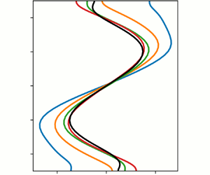
Figure 6 demonstrates how well the various levels of approximation reproduce the mean flow profiles (where the average is taken horizontally). Again, for straight convection, the means are poorly represented by the QL theories. However, as the separation of time scales becomes more pronounced and the EENL term becomes subdominant, GQL, even with $\varLambda =1$, provides an accurate representation of the saturated mean flow structures. It is precisely in these regimes that QL theories become effective, as predicted by the theory in § 2.1.

Figure 6. Results of QL/GQL simulations. Vertical ($z$) profiles of time and $(x,y)$-averaged $u$ velocity perturbations as a function of GQL cutoff $\varLambda$ for ${T_y}= -2, -0.5, 0$.

The QL approximation and its generalisations are examples of approximation via constrained triad decimation in pairs (Kraichnan Reference Kraichnan1985). The removal of certain interactions prevents certain routes for energy transfer. The effectiveness of the approximation presumably depends on how important these transfers were in the fully nonlinear DNS and how much damage removing them does to the dynamics and statistics of the system.

To reveal the preferred paths for transfer under the various degrees of approximation, we calculate energy transfer functions for the kinetic energy using methods outlined in Verma (Reference Verma2004), Alexakis, Mininni & Pouquet (Reference Alexakis, Mininni and Pouquet2005, Reference Alexakis, Mininni and Pouquet2007), Lesur & Longaretti (Reference Lesur and Longaretti2011), Favier, Silvers & Proctor (Reference Favier, Silvers and Proctor2014) and Currie & Tobias (Reference Currie and Tobias2020). Briefly, we calculate the transfer in horizontal wavenumber at a fixed $z$ location, so that each physical variable such as $q=q(x,y,z)$ has a corresponding Fourier transform $\tilde {q}=\tilde {q}(k_x,k_y,z)$. We denote a circular shell in Fourier space (e.g. pink in figure 1) where wavenumbers are near absolute value $K$

(5.1)\begin{equation} \textbf{K}\equiv \{{ (k_x,k_y) : K<\sqrt{k_x^2+k_y^2}\leq K+1 }\}.\end{equation}

This leads to a $K$-filtered representation

(5.2)\begin{equation} q_{K}(x,y,z)\equiv \sum_{\boldsymbol{k}\in\boldsymbol{\mathsf{K}}} \tilde{q}(k_x,k_y,z) \exp\left[{ 2{\rm \pi} {\rm i}\left({ {\frac{k_x x}{L_x}}+{\frac{k_y y}{L_y}} }\right) }\right], \end{equation}

which forms an orthogonal basis. Given the $K$-filtered vector velocity $\boldsymbol {u}_{K}\equiv (u_{K},v_{K},w_{K})$, the $K$-component of kinetic energy is $E_{K}={\frac 12}\boldsymbol {u}_{K}\boldsymbol {\cdot }\boldsymbol {u}_{K}$. The equation for $\partial E_{K}/\partial t$ leads to the energy ‘transfer function’ from modes at scale $Q$ to modes at a different scale $K$

(5.3)\begin{equation} \mathcal{T}(Q,K)\equiv{-}\iiint{\mathrm{d}\kern0.7pt x\,\mathrm{d}y\,\mathrm{d}z\,\boldsymbol{u}_{K} \boldsymbol{\cdot} (\boldsymbol{u}\boldsymbol{\cdot}\boldsymbol{\nabla})\boldsymbol{u}_{Q}}. \end{equation}

Vertically integrated transfer functions should ideally be antisymmetric about the line $Q=K$. In practice, the transfers at low $K$ and low $Q$ are noisy.

Figure 7 shows some examples of these $\mathcal {T}(Q,K)$ maps (temporally averaged); here the colour scales are proportional to absolute values, but coloured to indicate the sign (blue for $\mathcal {T}<0$; red for $\mathcal {T}>0$). Figure 7 shows these transfer functions for two different choices of ${T_y}=0, -2$ (${{Ra}}$ is fixed at the higher value of ${{Ra}} = 2 \times 10^5$) and two different choices of $\varLambda =0, 1$ and for DNS. In all cases the QL version cuts off most of the channels for interaction and so no cascades are available for energy transfer. Utilising GQL provides channels for non-local interactions and energy is scattered among modes.

Figure 7. Spectral transfer function $\mathcal {T}(k, p)$ between two wavenumbers $(k, p)$. Panels (a–c) show ${T_y} = 0$; (d–f) show ${T_y} = -2$.

The transfer function figure clearly shows that when $|{T_y}|$ is small, almost all transfers occurring in triad interactions between fluctuating modes and the EENL term are important. This is most obvious from the presence of energy transfer just above and below the diagonal. The local cascade is therefore dominant for turbulent flows with no mean flows. Note that in the case ${T_y}=0$, QL saturates via interaction of turbulent fluctuations with the mean flow (figure 7a), even though this is not the dominant mechanism in the DNS (c); the system has to saturate by altering the means, rather than utilising a cascade to increase dissipation.

However, when ${T_y}=-2$ nearly all of the energy is transferred via the mean flow in DNS; energy is transferred between turbulent modes in the cascade because of the interaction with the mean. It is this interaction that is more readily captured via QL descriptions; with GQL with $\varLambda =1$ giving a nearly perfect representation of the transfers for this case. A similar improvement in the accuracy of QL was found for the case of Langmuir turbulence which also breaks horizontal isotropy (Skitka, Marston & Fox-Kemper Reference Skitka, Marston and Fox-Kemper2020).