


Impact Statement
To the best of our knowledge, this is the first study to generate text discussions from images of numerical weather forecasts. We introduce (i) the largest benchmark dataset, comprising 1,367,041 image-text samples, to run experiments that explore the potential to generate text discussions from numerical weather prediction; and (ii) a methodology for evaluating generated text discussions of synoptic weather and climate.
1. Introduction
Recent advances in vision-language models (VLMs) have enabled substantial progress on complex multimodal tasks such as image captioning, document understanding, visual question answering (QA), and multimodal summarization. As these models improve in capability and are increasingly deployed or proposed for deployment in high-stakes settings, there is a growing need for evaluation frameworks that go beyond surface-level text similarity and instead quantify whether generated language is faithful, spatially grounded, and domain-relevant.
To this end, weather forecasting is a particularly consequential and technically challenging high-stakes domain. Numerical weather prediction (NWP) is deeply integrated into business operations, agriculture, government decision-making, public safety, and daily life for billions of people (Jones et al., Reference Jones, Hansen, Royce and Messina2000; World Meteorological Organization, 2015; Jain and Jain, Reference Jain and Jain2017; Uccellini and Ten Hoeve, Reference Uccellini and Ten Hoeve2019; Ukhurebor et al., Reference Ukhurebor, Adetunji, Olugbemi, Nwankwo, Akinola Samson Olayinka and Hefft2022). Vast observation networks and reanalysis products have enabled continual improvements in model development, data assimilation, and assessments of predictive reliability (Randles et al., Reference Randles, Da Silva, Buchard, Colarco, Darmenov, Govindaraju, Smirnov, Holben, Ferrare, Hair, Shinozuka and Flynn2017; Hersbach et al., Reference Hersbach, Bell, Berrisford, Hirahara, Horányi, Muñoz-Sabater, Nicolas, Peubey, Radu, Schepers, Simmons, Soci, Abdalla, Abellan, Balsamo, Bechtold, Biavati, Bidlot, Bonavita, De Chiara, Dahlgren, Dee, Diamantakis, Dragani, Flemming, Forbes, Fuentes, Geer, Haimberger, Healy, Hogan, Hólm, Janisková, Keeley, Laloyaux, Lopez, Lupu, Radnoti, Rosnay D, Rozum, Vamborg, Villaume and Thépaut2020). However, atmospheric dynamics are chaotic and span a wide range of spatial and temporal scales, which is why forecast verification relies on many complementary skill metrics (e.g., Anomaly Correlation Coefficient, RMSE, MAE, and skill scores) to characterize different aspects of performance (Brady and Spring, Reference Brady and Spring2021). In contrast, despite the operational importance of narrative forecasting products, methods to verifiably quantify the reliability of textual representations of atmospheric states and evolution remain limited.
Recent years have seen a growing body of work that explores multimodal learning for atmospheric data, including fine-tuning frontier VLMs and dataset creation for meteorological QA and event understanding. Examples include CLLMate (Li et al., Reference Li, Wang, Wang, Wang, Lau and Qu2024), which pairs extreme-event news with reanalysis for QA; RadarQA (He et al., Reference He, You, Gong, Liu, Yue, Zhuang, Zhang and Bai2025), which introduces radar annotations and heuristics for VLM fine-tuning; and hazard-focused datasets such as SEVIR (Veillette et al., Reference Veillette, Samsi, Mattioli, Larochelle, Ranzato, Hadsell, Balcan and Lin2020) and GridRad-Severe (Murphy et al., Reference Murphy, Homeyer and Allen2023). Additional efforts pair structured meteorological inputs with textual outputs for QA-oriented benchmarks, such as MeteorPred (Tang et al., Reference Tang, Xu, Zhang, Chen, Jin, Shen, Liu and Xiang2025), Climate IQA (Chen et al., Reference Chen, Zhou, Hua, Chong, Cao, Li, Chen, Zhu, Liang and Yuan2025), Zephyrus (Varambally et al., Reference Varambally, Fisher, Thakker, Chen, Xia, Jafari, Niu, Jain, Manivannan, Novack, Han, Eranky, Cachay, Berg-Kirkpatrick, Watson-Parris, Ma and Yu2025), and WeatherQA (Ma et al., Reference Ma, Hua, Anderson-Frey, Iyer, Liu and Qin2024). While these studies demonstrate the promise of multimodal models for atmospheric applications, direct comparisons across benchmarks are often confounded by rigid constraints on target outputs, spatial scales, forecast horizons, and training data choices. Moreover, many evaluations emphasize QA accuracy or rely heavily on traditional text metrics (Bleu, Rouge, Meteor, BertScore) and/or LLM-judge scoring, which can be insufficient for assessing whether generated discussions correctly identify synoptic phenomena, capture their spatial extent, and reflect scale-dependent relevance to a forecast domain.
1.1. Present work
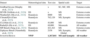
To address all the aforementioned gaps, we introduce a new benchmark and evaluation methodology designed specifically for the generation and verification of synoptic-scale forecast discussions. We present SynopticBench, a large-scale dataset comprising 1,367,041 National Weather Service (NWS) Area Forecast Discussions paired with forecast images of 500 mb geopotential height, 2 m temperature, and 850 mb wind velocity over the continental United States. In contrast to existing benchmarks, SynopticBench is the first benchmark to evaluate NWP meteorological samples across both mesoscale and synoptic spatial scales for all weather (see Table 3). Critically, we also propose Synoptic Phenomena Alignment and Coverage Evaluation (Space), an evaluation framework that explicitly accounts for the scale-dependent nature of atmospheric phenomena and the differing spatial precision required across variables (e.g., precipitation versus pressure patterns). Space is designed to evaluate distinct phenomena separately while incorporating spatial coverage and relevance, enabling more faithful estimation of a VLM’s skill in generating meteorological text. Building on SynopticBench, we train models for synoptic discussion generation and fine-tune widely used VLMs. Our results show that the ability of the models to conduct physical reasoning is improved from fine-tuning. The key goal of SynopticBench is to advance the study and understanding of VLMs in weather forecasting. Therefore, we share the dataset, metric, and fine-tuned weights of a range of VLMs to support reproducible research and more rigorous, domain-appropriate evaluation of VLMs in weather forecasting (Table 1).
Comparison between SynopticBench and existing work using multimodal datasets for atmospheric data
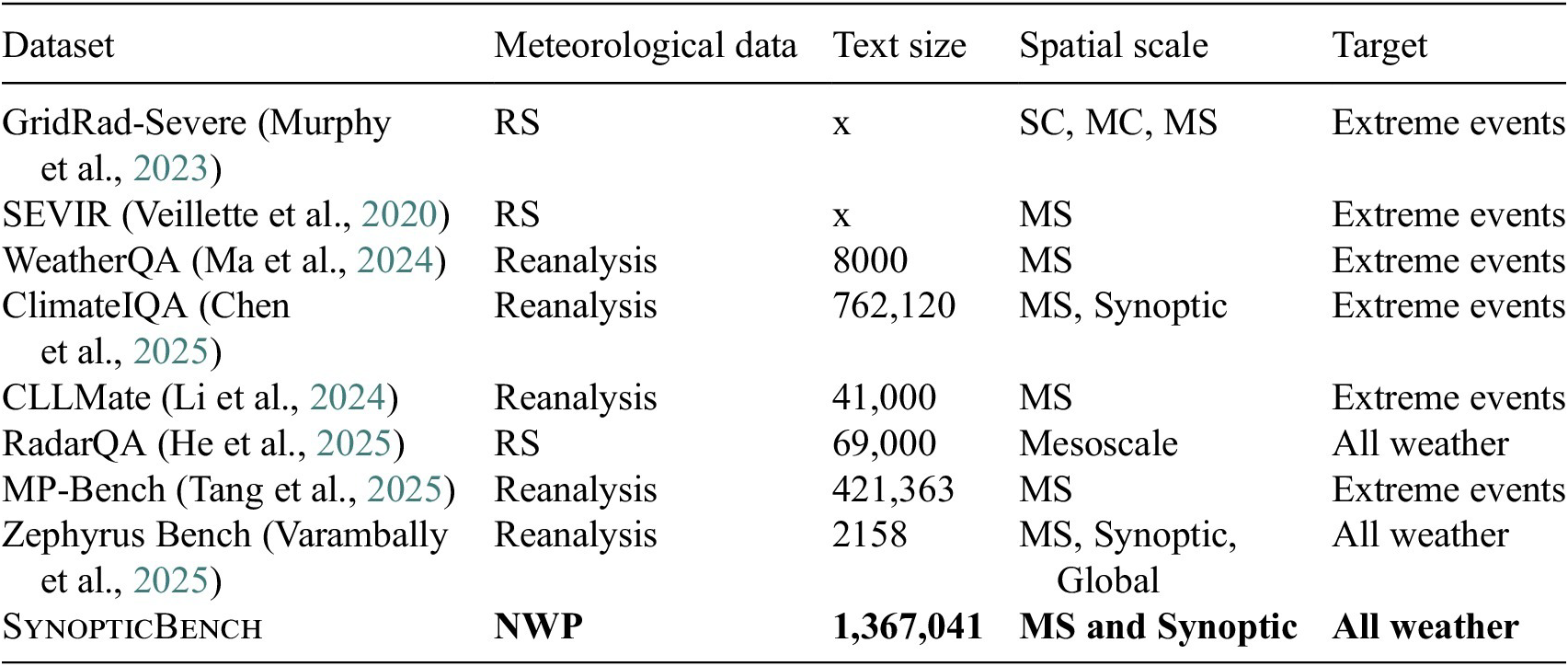
Table 1. Long description
The table consists of five columns: Dataset, Meteorological data, Text size, Spatial scale, and Target.
* GridRad-Severe (Murphy et al., 2023): RS data, text size x, spatial scales SC, MC, MS, targeting Extreme events.
* SEVIR (Veillette et al., 2020): RS data, text size x, spatial scale MS, targeting Extreme events.
* Weather QA (Ma et al., 2024): Reanalysis data, text size 8000, spatial scale MS, targeting Extreme events.
* Climate IQA (Chen et al., 2025): Reanalysis data, text size 762,120, spatial scales MS and Synoptic, targeting Extreme events.
* CLLMate (Li et al., 2024): Reanalysis data, text size 41,000, spatial scale MS, targeting Extreme events.
* Radar QA (He et al., 2025): RS data, text size 69,000, spatial scale Mesoscale, targeting All weather.
* MP-Bench (Tang et al., 2025): Reanalysis data, text size 421,363, spatial scale MS, targeting Extreme events.
* Zephyrus Bench (Varambally et al., 2025): Reanalysis data, text size 2158, spatial scales MS, Synoptic, and Global, targeting All weather.
* SynopticBench: NWP data, text size 1,367,041, spatial scales MS and Synoptic, targeting All weather.
Note: RS stands for Remote sensing, NWP for Numerical weather prediction, SC for Single-cell, MC for Multi-cell, and MS for Mesoscale.
Note. Here, we present the type of meteorological data (RS
$ \to $
 Remote sensing; NWP
$ \to $
Remote sensing; NWP
$ \to $
 Numerical weather prediction), the number of text samples, the relevant spatial scales (SC
$ \to $
Numerical weather prediction), the number of text samples, the relevant spatial scales (SC
$ \to $
 Single-cell; MC
$ \to $
Single-cell; MC
$ \to $
 Multi-cell; MS
$ \to $
Multi-cell; MS
$ \to $
 Mesoscale), and the target of each study. SynopticBench is the first large-scale benchmark that generates text from NWP and contains 1,367,041 text samples.
2. SynopticBench
Here, we detail the dataset building pipeline (Section 2.1), data collection (Section 2.2), data preprocessing (Section 2.3), and our proposed Space metric (Section 2.5).
2.1. Dataset building pipeline
One of the largest bottlenecks that stunts progress for multimodal models for atmospheric data is the scarcity of high-quality text that can be paired with numerical data. We propose using Area Forecast Discussions (AFDs) created by the NWS as a potential solution to the multimodal data problem. The AFD text data are publicly available and were extracted from the Iowa Environmental Mesonet (https://mesonet.agron.iastate.edu/wx/afos/list.phtml). AFDs exist at NWS stations across the United States and are typically issued multiple times per day. They reliably describe weather forecasts to an exceptionally high degree of detail, often informing the public about the weather a week in advance (National Research Council, 2006). In addition, they describe numerous physical variables, vertical levels, spatial scales, and processes. AFDs also typically include high-quality descriptions of the temporal evolution of weather phenomena, creating potential for training models to generate text that describes how atmospheric data changes over time.
2.2. Dataset collection
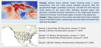
We create SynopticBench by pairing the National Centers for Environmental Prediction (NCEP) Global Forecast System (GFS) model (National Centers for Environmental Prediction/National Weather Service/NOAA/U.S. Department of Commerce, 2015) to AFDs. This dataset contains GFS forecasts issued four times per day from January 1, 2016, to December 31, 2025 (14,159 total forecasts) paired with 1,367,041 AFD text samples. Each GFS forecast consists of 2 m temperature, precipitation rate, 500 mb geopotential height, 850 mb zonal wind, and 850 mb meridional wind that is matched to the nearest AFD in time (always within several hours) for each location. We pair each forecast with 117 text samples, as there are 117 NWS station locations used in the study ( Figure 1 ). This creates consistency among the text samples for descriptions of the primary synoptic features occurring over the US for a given forecast.
An example case of a single sample from the training set (top panel). Each training sample image has a yellow box indicating the location of the discussion. The example answer is a filtered AFD. All of the locations used in the discussions are shown in the bottom panel. The format of the training samples is also shown, with 117 AFDs matched to each forecast.
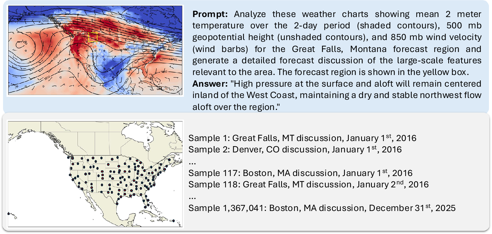
Figure 1. Long description
The top panel contains a meteorological map of North America on the left, displaying shaded temperature contours in red and blue, unshaded geopotential height lines, and wind barbs. A small yellow box is centered over Montana. To the right of the map is a text block labeled Prompt, which asks for an analysis of the weather charts for Great Falls, Montana, followed by an Answer providing a forecast discussion. The bottom panel features a map of the United States on the left with numerous black dots indicating data collection locations across the country. To the right is a vertical list of training samples. Sample 1 is Great Falls, MT discussion, January 1st, 2016. Sample 2 is Denver, CO discussion, January 1st, 2016. The list continues to Sample 117 for Boston, MA, then Sample 118 for Great Falls on January 2nd, 2016, and concludes with Sample 1,367,041 for Boston, MA, December 31st, 2025.
2.3. Preprocessing
Before we begin training and evaluating VLMs, we apply several data preprocessing steps to both AFDs and GFS forecasts. During preprocessing, we first discard all lead times beyond 48 hours. Although AFDs primarily align with GFS forecasts, they are sometimes based on other models as well, which diverge as the lead time increases due to the chaotic nature of the atmosphere. The spatial domain is cropped from 15°N to 65°N and 60°W to 160°W. We plot mean 2 m temperature anomalies in shaded contours along with mean 500 mb geopotential height in line contours and 850 mb wind velocity in the form of wind barbs. A yellow 5°
$ \times $
 5° box is centered on the location of each discussion that is paired to an image.
Keeping the goal of matching text that can be represented in the images, we preprocessed the information in the AFDs for the experiments. AFDs are often informed by GFS forecasts but can use information from a variety of different models. We remove sentences including any reference to other forecast models or synoptic pressure systems that do not exist at the scale or vertical level that the images show. We also only use sentences including keywords that do describe synoptic pressure systems and temperature anomalies including trough, ridge, low pressure, high pressure, cold front, and warm front. The full list of inclusion and exclusion keywords is included in the Supplementary Appendix. When evaluating synoptic phenomena with lead times up to 48 hours, we can also expect robust consistency of large-scale patterns. The information described in AFDs occurs chronologically, often including the day of the week on which different phenomena occur. Once a day of the week that is more than two days after the issue day is mentioned, all text that follows is removed to stay consistent with the forecast lead times.
2.4. Baselines
We used four different baselines to add perspective to the results. Gemini-3.1 Pro is used as a baseline for current state-of-the-art models. The nearest neighbor baseline is created by first computing the SSIM scores between each test set image and all training set images. The text paired with the training set image with the highest SSIM score is used as the text for each sample in the baseline. The climatology is created by choosing text from a random sample in the training set from the same month and location as each sample in the test set. The blind LLM baseline strips the image tokens from test before running LLaMA-3.2-11B.
2.5. Synoptic phenomena alignment and coverage evaluation (Space) metric
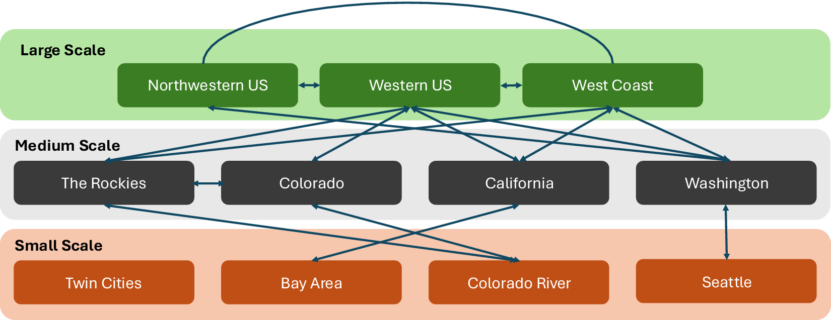
Traditional metrics for text evaluation are not sufficient for text describing atmospheric processes because they do not include any physical reasoning. The purpose of Space is to evaluate the ability of the VLM to generate text that predicts the correct phenomenon in the target location. Evaluating location accuracy from text can be a complex task because many terms may differ entirely but represent similar locations (e.g., The Rockies versus Colorado) and the precision of location terms may be more or less acceptable depending on the scale of the phenomenon (e.g., “trough moving through the Denver area” vs. “trough moving through Colorado” is preferred more than “rain in the Denver area” vs. “rain in Colorado”). To accommodate these relations, we introduce a spatial hierarchy tree specifically created for evaluating text describing synoptic phenomena. The hierarchy comprises three levels that capture terms commonly used to detail the locations of synoptic weather phenomena in North America (see Figure 2 for an example of a small portion of the hierarchy tree).
Several examples of matching large- (green), medium- (purple), and small-scale (orange) location keywords. Blue lines indicate the potential matches that these locations would make if found in the predicted or reference text.
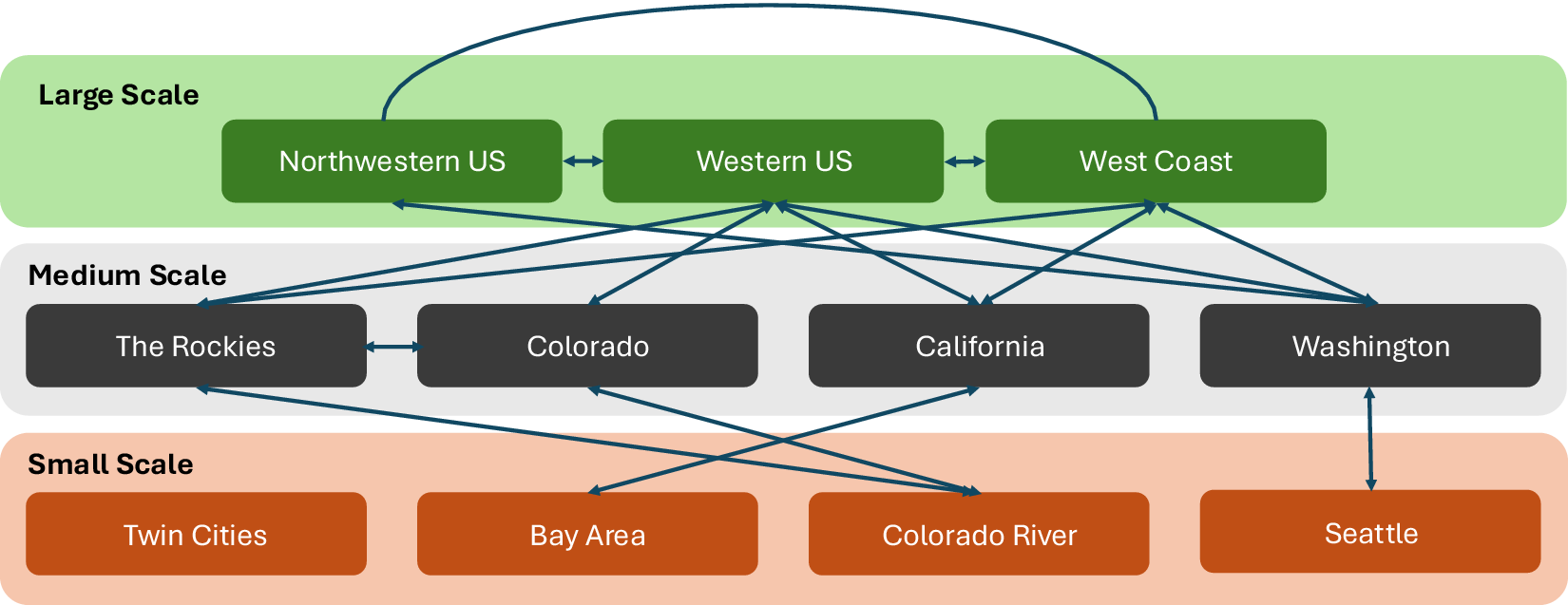
Figure 2. Long description
The diagram is organized into three horizontal bands representing different geographic scales.
At the top is the Large Scale band in light green. It contains three dark green nodes: Northwestern US, Western US, and West Coast. Horizontal double-headed arrows connect Northwestern US to Western US, and Western US to West Coast. A curved blue line also connects Northwestern US directly to West Coast.
The middle band is Medium Scale in light gray. It contains four dark gray nodes: The Rockies, Colorado, California, and Washington. A horizontal arrow connects The Rockies and Colorado. This layer is heavily interconnected with the Large Scale layer above. Northwestern US points to The Rockies and Washington. Western US points to The Rockies, Colorado, California, and Washington. West Coast points to California and Washington.
The bottom band is Small Scale in light orange. It contains four dark orange nodes: Twin Cities, Bay Area, Colorado River, and Seattle. Inter-layer connections include Colorado in the Medium Scale pointing to Colorado River in the Small Scale. California points to the Bay Area. Washington points to Seattle. Additionally, Western U S from the top layer points directly down to the Colorado River and Bay Area nodes.
Space can be applied toward various types of synoptic weather phenomena that have positive and negative phase categorizations (e.g., high/low pressure systems, warm/cold fronts, wet/dry events). Next, to demonstrate the methodology of Space, we use pressure systems as an example. We begin Space by matching pressure terms to locations. If “low pressure,” “high pressure,” “trough” (excluding instances of “shortwave trough”), or “ridge” exists in the text, the term is first matched to any location that follows in the sentence. For a sample of text, this creates a list of pressure systems matched to different locations. Pressure terms are then matched to other instances for locations that are equal or related (see connections in
Figure 2
). Locations with a common relative can also match with the exception of those that cover a large portion of the continent (see Supplementary Appendix). This logic creates groups of pressure objects for both the generated and the AFD text sample. Objects can be grouped for single discussions (Space-local) or aggregated across all locations (Space-aggregate) for a single forecast. If any object from a group has the same pressure sign and a location related to any object in the corresponding text sample, the object groups form a match. We consider “trough” to be synonymous with “low pressure,” and “ridge” to be synonymous with “high pressure.” The match score,
$ {s}_m $
 , is a measure of the quality of the matches and is defined below:
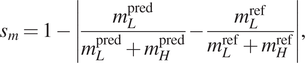
where
$ {m}_L^{\mathrm{pred}} $
 is the number of matching negative phase objects in the predicted text,
$ {m}_L^{\mathrm{ref}} $
is the number of matching negative phase objects in the predicted text,
$ {m}_L^{\mathrm{ref}} $
 is the number of matching negative phase objects in the reference text,
$ {m}_H^{\mathrm{pred}} $
is the number of matching negative phase objects in the reference text,
$ {m}_H^{\mathrm{pred}} $
 is the number of matching positive phase objects in the predicted text, and
$ {m}_H^{\mathrm{ref}} $
is the number of matching positive phase objects in the predicted text, and
$ {m}_H^{\mathrm{ref}} $
 is the number of matching positive phase objects in the reference text. The coverage ratio,
$ {r}_c $
is the number of matching positive phase objects in the reference text. The coverage ratio,
$ {r}_c $
 , is the percentage of pressure objects that are included in matches and is defined as:

where
$ {n}_L $
 is the total number of negative phase objects and
$ {n}_H $
is the total number of negative phase objects and
$ {n}_H $
 is the total number of positive phase objects in the combined predicted and observed text. The coverage ratio is designed to penalize the generated text for creating hallucinations and for failing to mention key terms. The final Space score is calculated as the product of the matching score and coverage ratio, that is,
$ s={s}_m\cdot {r}_c $
is the total number of positive phase objects in the combined predicted and observed text. The coverage ratio is designed to penalize the generated text for creating hallucinations and for failing to mention key terms. The final Space score is calculated as the product of the matching score and coverage ratio, that is,
$ s={s}_m\cdot {r}_c $
 .
.
3. Results
3.1. Traditional metrics are not sufficient
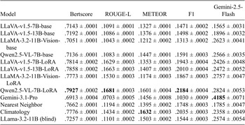
Base model versions for LLaVA-v1.5-7B, LLaVA-v1.5-13B, Qwen2-VL-7B, and LLaMA-3.2-11B-Vision were run on the test set. We first evaluate each of the four base models, fine-tuned models, and baselines on traditional skill metrics (Table 2). LoRA fine-tuning improved performance on all traditional metrics except METEOR for LLaMA-3.2-11B-Vision. The climatology baseline had the highest METEOR score, while fine-tuned Qwen2.5-VL-7B had the highest Bertscore, ROUGE-L, and F1 scores. Gemini-3.1-Pro had the lowest Bertscore, ROUGE-L score, METEOR score, and F1 score while having the highest LLM-as-a-judge score. The climatology baseline used text from real NWS AFDs issued from the same exact station, which may have allowed it to have relatively high scores for traditional metrics by using similar discussion styles. Despite slight variations in the performance of all models, all scores were low, indicating that the language in the generated discussions had little overlap with the NWS discussions. The traditional scores cannot determine the models’ ability to discuss the primary relevant features in the images, which creates a need for further evaluation.
Traditional metrics for base models, fine-tuned models, and baselines are shown
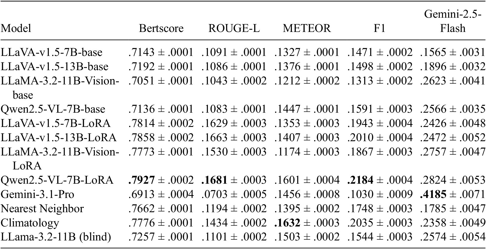
Table 2. Long description
The table contains six columns: Model, Bertscore, ROUGE dash L, METEOR, F1, and Gemini dash 2 dot 5 dash Flash. Data is presented as mean plus or minus standard error.
* LLaVA dash v1 dot 5 dash 7B dash base: Bertscore .7143, ROUGE dash L .1091, METEOR .1327, F1 .1471, Gemini .1565.
* LLaVA dash v 1 dot 5 dash 13B dash base: Bertscore .7192, ROUGE dash L .1086, METEOR .1376, F1 .1498, Gemini .1896.
* LLaMA dash 3 dot 2 dash 11B dash Vision dash base: Bertscore .7051, ROUGE dash L .1043, METEOR .1212, F 1 .1313, Gemini .2623.
* Qwen 2 dot 5 dash VL dash 7B dash base: Bertscore .7136, ROUGE dash L .1083, METEOR .1447, F1 .1591, Gemini .2566.
* LLaVA dash v 1 dot 5 dash 7B dash L o RA: Bertscore .7814, ROUGE dash L .1629, METEOR .1353, F1 .1943, Gemini .2426.
* LLaVA dash v 1 dot 5 dash 13B dash L o RA: Bertscore .7858, ROUGE dash L .1663, METEOR .1407, F1 .2010, Gemini .2472.
* LLaMA dash 3 dot 2 dash 11B dash Vision dash L o RA: Bertscore .7773, ROUGE dash L .1530, METEOR .1174, F1 .1867, Gemini .2757.
* Qwen 2 dot 5 dash VL dash 7B dash L o RA: Bertscore .7927, ROUGE dash L .1681, METEOR .1601, F1 .2184, Gemini .2824. This model has the highest Bertscore, ROUGE dash L, and F1 among the fine-tuned models.
* Gemini dash 3 dot 1 dash Pro: Bertscore .6913, ROUGE dash L .0703, METEOR .1456, F1 .1030, Gemini .4185. This model has the highest Gemini dash 2 dot 5 dash Flash score.
* Nearest Neighbor: Bertscore .7662, ROUGE dash L .1194, METEOR .1395, F1 .1748, Gemini .1785.
* Climatology: Bertscore .7776, ROUGE dash L .1434, METEOR .1632, F1 .2035, Gemini .2358. This model has the highest METEOR score.
* LLaMA dash 3 dot 2 dash 11B blind: Bertscore .7257, ROUGE dash L .1101, METEOR .1503, F1 .1544, Gemini .2574.
Note. We calculate the mean and standard error of the mean Bertscore, ROUGE-L, METEOR, F1, and LLM-judge scores across samples within the test set. The range of possible scores for all metrics is 0–1, with 1 being a perfect score.
The bold values are the highest value for each column.
3.2. Space scores can reduce evaluation uncertainty
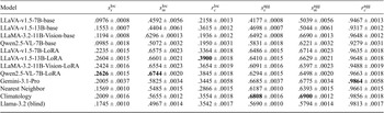
Although Space could be used for various types of weather phenomena, we demonstrate the utility of Space on pressure systems in this study. Here, we show how Space scores can help the user understand how each model performs in identifying the correct relevant pressure systems for the area and referring to them in the correct locations. Space-aggregate uses all locations at a given time to create a large sample size of pressure objects matched to specific locations for evaluation. It is useful for understanding the model’s ability to determine the general large-scale pressure features that occur in the forecast. Space-local uses a single location at a given time to create a much smaller sample size of pressure objects but can be useful for understanding the model’s ability to discuss the features impacting a specific location. All Space scores for pressure systems are shown in Table 3. Space-aggregate scores are considerably higher than Space-local scores because the increased sample size of text increases the chances that relevant locations for synoptic phenomena are mentioned in both the generated text and the AFDs. Theoretically, a model that always randomly guesses between high pressure and low pressure would have a match score of roughly 0.5 without any knowledge of climatology, which indicates that the fine-tuned models likely all have some skill in distinguishing between high and low pressure. The local coverage ratios (
$ {r}_c $
 ) are lower than the match scores for every model, demonstrating that predicting the phenomena in the correct location is a more challenging task for these VLMs than accurately describing the correct polarity of synoptic phenomena.
SPACE was used for synoptic pressure system evaluation for base models, fine-tuned models, and baselines
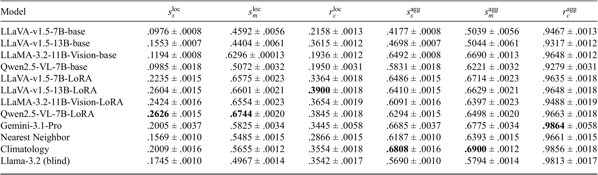
Table 3. Long description
The table consists of 7 columns and 13 rows. The columns are labeled: Model, s sub s super loc, s sub m super loc, r sub c super loc, s sub s super agg, s sub m super agg, and r sub c super agg.
* LLaVA-v1.5-7B-base: .0976 plus or minus .0008, .4592 plus or minus .0056, .2158 plus or minus .0013, .4177 plus or minus .0008, .5039 plus or minus .0056, .9467 plus or minus .0013.
* LLaVA-v1.5-13B-base: .1553 plus or minus .0007, .4404 plus or minus .0061, .3615 plus or minus .0012, .4698 plus or minus .0007, .5044 plus or minus .0061, .9317 plus or minus .0012.
* LLaMA-3.2-11B-Vision-base: .1194 plus or minus .0008, .6296 plus or minus .00013, .1936 plus or minus .0012, .6492 plus or minus .0008, .6690 plus or minus .0013, .9648 plus or minus .0012.
* Qwen2.5-V L-7B-base: .0985 plus or minus .0018, .5072 plus or minus .0032, .1950 plus or minus .0031, .5831 plus or minus .0018, .6221 plus or minus .0032, .9279 plus or minus .0031.
* LLaVA-v1.5-7B-LoRA: .2235 plus or minus .0015, .6575 plus or minus .0023, .3364 plus or minus .0018, .6486 plus or minus .0015, .6714 plus or minus .0023, .9635 plus or minus .0018.
* LLaVA-v1.5-13B-LoRA: .2604 plus or minus .0015, .6601 plus or minus .0021, bold .3900 plus or minus .0018, .6410 plus or minus .0015, .6629 plus or minus .0021, .9648 plus or minus .0018.
* LLaMA-3.2-11B-Vision-LoRA: .2424 plus or minus .0016, .6554 plus or minus .0023, .3654 plus or minus .0019, .6091 plus or minus .0016, .6397 plus or minus .0023, .9488 plus or minus .0019.
* Qwen2.5-V L-7B-LoRA: bold .2626 plus or minus .0015, bold .6744 plus or minus .0020, .3845 plus or minus .0018, .6294 plus or minus .0015, .6498 plus or minus .0020, .9663 plus or minus .0018.
* Gemini-3.1-Pro: .2005 plus or minus .0037, .5825 plus or minus .0034, .3445 plus or minus .0058, .6685 plus or minus .0037, .6775 plus or minus .0034, bold .9864 plus or minus .0058.
* Nearest Neighbor: .1569 plus or minus .0010, .5485 plus or minus .0015, .2866 plus or minus .0015, .6187 plus or minus .0010, .6393 plus or minus .0015, .9661 plus or minus .0015.
* Climatology: .2009 plus or minus .0016, .5655 plus or minus .0012, .3554 plus or minus .0018, bold .6808 plus or minus .0016, bold .6900 plus or minus .0012, .9856 plus or minus .0018.
* Llama-3.2 blind: .1745 plus or minus .0010, .4967 plus or minus .0014, .3542 plus or minus .0017, .5690 plus or minus .0010, .5794 plus or minus .0014, .9813 plus or minus .0017.
Note. We calculate the mean and standard error of the SPACE-local and SPACE-aggregate scores (
$ {s}_s $
 ), match scores (
$ {s}_m $
), match scores (
$ {s}_m $
 ), and coverage ratios (
$ {r}_c $
), and coverage ratios (
$ {r}_c $
 ) within the test set. The range of possible scores for all metrics is 0 to 1, with 1 being a perfect score.
The bold values are the highest value for each column.
The Qwen2.5-VL-7B fine-tuned model had the highest Space-local scores, while Climatology had the highest Space-aggregate scores. The fine-tuned models had higher Space-local scores than all of the base models and baselines. The Space-aggregate scores for the fine-tuned models were generally higher than those of the base models with the exception of LLaMA-3.2-11B-Vision. The improvement of Space-aggregate scores over base models is impacted by both improved coverage ratios and match scores. The Space scores often agree with the traditional metrics, with the fine-tuned Qwen-VL-7B configuration generally having the highest scores. One clear exception is Gemini-3.1-Pro, which has some of the lowest scores when evaluated on traditional metrics and fairly high Space scores. The Space scores and traditional metrics also suggest that increasing the parameters from 7 billion to 13 billion in LLaVA does not drastically improve generated discussion quality and the fine-tuning approach is far more effective.
3.3. Case studies illustrate the advantages of Space
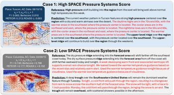
An example of the evaluation of both Space and traditional metrics in two different cases is shown in Figure 3. In Case 1, there is a high-pressure system over the southwestern United States, which is the most influential pressure system relevant to the station location (Tuscon, Arizona). The NWS discussion mentions high pressure in the region, and the generated VLM text also discusses high-pressure systems in the same region. This leads to a perfect Space-local score for pressure systems. The traditional metrics for this case were generally close to average for this model. In Case 2, there is a high-pressure system over much of the southeastern US, which is the most influential pressure system to the station location (Columbia, South Carolina). The NWS discussion mentions a ridge in the forecast area while the VLM’s generated text discusses a trough in the southeastern United States. This leads to a Space score of 0. Despite having a Space-local score of 0, the traditional metrics were unable to show a clear difference in the quality of both cases. Case 2 also shows some instances of hallucinations in which the model discusses phenomena that it could not possibly see based on the image (e.g., 1 inch of snow), which does not penalize the Space score because Space only evaluates one type of phenomenon at a time. This case study demonstrates a clear example of the reliability of Space scores relative to traditional metrics for the evaluation of individual types of phenomena in weather discussions. Several additional cases are shown in the Supplementary Appendix.
Two cases demonstrating differences between Space scores and traditional skill metrics. The reference text samples are filtered NWS AFDs, and the prediction text samples are generated from the fine-tuned version of LLaVA-v1.5-7B. The terms in bold are used to compute Space scores for pressure systems. Sentences that are irrelevant to the Space scores are shown in red.
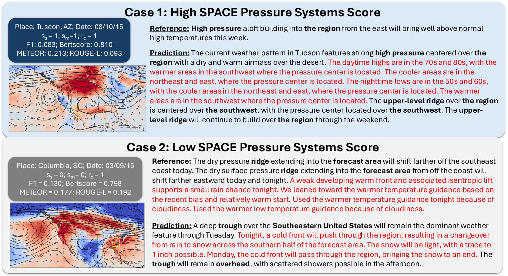
Figure 3. Long description
The image consists of two horizontal panels labeled Case 1 and Case 2.
Case 1: High SPACE Pressure Systems Score.
- Left side: Metadata for Tucson, AZ on August 10, 2015. Metrics include s sub s = 1, s sub m = 1, r sub c = 1, F1 = 0.083, Bertscore = 0.810, METEOR = 0.213, and ROUGE-L = 0.093. Below this is a weather map showing a large red high-pressure ridge over the Southwestern United States.
- Right side: Reference text describes high pressure building into the region. Prediction text correctly identifies high pressure over the region and the southwest, though it contains several redundant sentences in red regarding temperature and pressure center locations.
Case 2: Low SPACE Pressure Systems Score.
- Left side: Metadata for Columbia, SC on March 9, 2015. Metrics include s sub s = 0, s sub m = 0, r sub c = 1, F1 = 0.130, Bertscore = 0.798, METEOR = 0.177, and ROUGE-L = 0.192. Below this is a weather map showing a blue low-pressure trough over the Eastern United States.
- Right side: Reference text describes a dry pressure ridge shifting off the southeast coast. Prediction text incorrectly identifies a deep trough over the Southeastern United States and mentions a cold front with rain and snow in red text, which contradicts the reference’s ridge description.
4. Conclusion
In this work, we introduce a dataset with more than one million samples that we use to train a VLM for discussion generation from images of weather forecasts across North America. We also introduce a skill metric (Space) to evaluate the ability of language models to identify important synoptic features in the correct locations. Fine-tuning VLM projector weights with LoRA adapters leads to greater overall performance than the base models on both Space and traditional metrics. Climatology and fine-tuned Qwen2.5-VL-7B had the highest scores in most of the metrics in this study, with Qwen2.5-VL-7B excelling more in describing features relevant to a precise location. The failure of any model to score higher than climatology in the Space-aggregate scores demonstrates a key limiting factor in the ability of the models in this study to accurately describe synoptic features throughout the entire system.
The dataset used in this study pairs highly complex forecast discussions from the NWS with images of weather forecasts. This study performed experiments on synoptic pressure systems as an example use case and focused entirely on the United States, which creates an opportunity for future work. Human expert evaluation for text describing various types of atmospheric phenomena would also be valuable for strengthening confidence in any current or future metrics. The size and complexity of the dataset allow the user to perform experiments on other types of phenomena, specific locations or regions, spatial scales, and temporal ranges. Although the fine-tuned models often outperformed the base models on Space scores, improved model architectures and loss functions, agentic frameworks, and video-language models could add additional benefits.
Weather forecasts are highly complex, and complete descriptions of them therefore often require long and detailed discussions. None of the models used in this study comes close to rivaling the reliability nor complexity of NWS AFDs, so the evaluation of text generation for weather and climate applications must begin with basic isolated tasks. Space scores excel in capturing similarities in some of the most important details of text samples. They can help evaluate the ability of the models to demonstrate physical understanding of atmospheric processes rather than only learning common textual patterns. By determining the ability of the model to do so, the user can better understand when to stop training, which can help prevent overfitting.
Although Space scores are a useful method for evaluating text for multimodal language models for weather and climate applications, they do not fully capture the level of quality in generated forecast discussions, and additional metrics that evaluate text would help create a more comprehensive evaluation framework. Future improvements could involve temporal accuracy (more relevant for longer lead times), system evolution (more relevant for models that can handle videos), and vertical levels (more relevant for models that can handle more channels).
Supplementary material
The supplementary material for this article can be found at http://doi.org/10.1017/eds.2026.10050.
Acknowledgments
The authors thank the reviewers of this work for their dedication toward supporting the research community and providing comments that were critical toward improving the manuscript.
Author contribution
Conceptualization, Investigation, Methodology, Project administration, Validation and Writing - review & editing: T.H., A.M., and C.A.; Data curation, Formal analysis, Software, Visualization and Writing - original draft: T.H.; Funding acquisition, Resources, Supervision: A.M., and C.A. T.H., A.M., and C.A. contributed new analytic metrics and wrote the manuscript. T.H. wrote all the codes, retrieved, processed, and harmonized datasets, and performed the analyses for technical validation of the new resource. A.M. and C.A. conceived the study.
Competing interests
The author declare none.
Data availability statement
The code used to conduct this study can be found at Higgins (Reference Higgins2026). The dataset can be found here: https://huggingface.co/datasets/Aikyam-Lab/Synoptic-Bench.
Author contribution
Conceptualization, Investigation, Methodology, Project administration, Validation and Writing - review & editing: T.H., A.M., and C.A.; Data curation, Formal analysis, Software, Visualization and Writing - original draft: T.H.; Funding acquisition, Resources, Supervision: A.M., and C.A.
Ethics statement
The research meets all ethical guidelines, including adherence to the legal requirements of the study country.
Funding statement
This work was funded by the University of Virginia Environmental Institute Climate Fellows Program Grant DN002057.
Provenance statement
This article is part of the Climate Informatics 2026 proceedings and was accepted in Environmental Data Science on the basis of the Climate Informatics peer-review process.


 Open access

