

Introduction
The present increase in global temperatures has been associated with human activities, and the increase has been projected to accelerate in the next 100 years (Reference HoughtonHoughton and others, 2001). However, it is imperative to understand the natural variability of climate to assess the human impact and make better predictions of future climates. In a sense, the Holocene climate is the key to the future (personal communication from R.S. Bradley, 2006). Direct observations or indirect geological/geomorphological evidences of glacier fluctuations have been one of the main sources of information about past climate variability in the northern high latitudes in the past (e.g. Reference Karlén, Mörner and KarlénKarlén, 1984; Reference LuckmanLuckman, 1993). Before aerial photographs or satellite images came into use, direct observations were made during the occasional survey of mountainous areas or in connection with specific changes of a glacier (e.g. a rapid advance of a valley glacier). These ‘snapshots’ of glacier volume provide valuable information, but the mechanism behind the observed change is difficult to assess. Using geological/geomorphological evidence, such as terminal moraines or proglacial lacustrine sediments, it is possible to attain chronologies of (at least relative) glacier fluctuations. Lichenomertry can provide estimates of when moraines were formed, and moraines and sediments (if they contain organic matter) can be dated by the 14C method (Reference Karlén and DentonKarlén and Denton, 1976) or dendrochronological methods (Reference LuckmanLuckman, 1993; Reference Carter, LeRoy, Nelson, Laroque and SmithCarter and others, 1999). Historical records (e.g. written records or photographs) can be used to date certain events. Together, these indicators yield information on past glacier fluctuations, but usually with large uncertainty regarding the timing of events. This, in turn, results in uncertainties regarding the rate of change, and it may be difficult to set the glacier changes into proper climatological context. To fully understand how glaciers respond to climate variability and to interpret past changes as well as infer glacier responses to future climate change, high-resolution records of glacier fluctuations are needed.
Direct measurements of glacier mass balance provide a detailed picture of the volume change of glaciers. Measurement methods vary, but the records provide means to compare glacier variability to measured meteorological parameters. Unfortunately, the majority of mass-balance records are short, and very few span more than 50 years. To extend these records back in time, proxies for the mass balance with similar high time resolution are needed.
In cases where the summer balance variability dominates the net balance variability, proxies for summer ablation, such as tree rings, have been used to reconstruct glacier mass balance (Matthews, 1977; Reference Karlén, Mörner and KarlénKarlén, 1984; Reference NicolussiNicolussi, 1994; Reference Lewis and SmithLewis and Smith, 2004). Mass-balance variations, especially winter balance, have also been linked to large-scale atmospheric changes rather than just single meteorological parameters (Reference Walters, Meier and PetersonWalters and Meier, 1989; Reference Pohjola and RogersPohjola and Rogers, 1997a, Reference Pohjola and Rogersb; Reference Hodge, Trabant, Krimmel, Heinrichs, March and JosbergerHodge and others, 1998; Reference McCabe, Fountain and DyurgerovMcCabe and others, 2000; Reference Nesje, Lie and DahlNesje and others, 2000). However the lack of long, high-resolution atmospheric circulation records has resulted in only few attempts to reconstruct glacier mass balance using such data (e.g. Reference Nordli, Lie, Nesje and BenestadNordli and others, 2005; Reference Linderholm, Jansson and ChenLinderholm and others, 2007).
Reconstructions based on either summer or winter conditions should in general be viewed as approximations. Furthermore, such reconstructions rely on the assumption that the relationship between net balance and summer or winter balance (i.e. summer temperatures or winter precipitation) is stationary, which is not certain, as has been shown for Storglaciären, northern Sweden, by Reference HolmlundHolmlund (1987), for example. To obtain more reliable reconstructions, winter and summer balances should be reconstructed separately. In recent years, new reconstructions of glacier mass balance have appeared where the approach is similar to that of the actual in situ measurements of glacier mass balance, i.e. separate treatment of summer and winter balance. Reference Nordli, Lie, Nesje and BenestadNordli and others (2005) modelled glacier mass balance in southern Norway back to 1781 using circulation indices, based on monthly mean sea-level pressure (MSLP) data for winter balance, and spring–summer temperatures (partly deduced from farmers’ diaries) for summer balance. The same approach was used in northern Sweden by Reference Linderholm, Jansson and ChenLinderholm and others (2007), but with tree-ring data as the summer balance proxy. In North America, Reference Watson and LuckmanWatson and Luckman (2004) and Reference Larocque and SmithLarocque and Smith (2005) both used dendrochronological data to infer summer and winter balances separately.
In this paper, we take a similar approach to that of Reference Linderholm, Jansson and ChenLinderholm and others (2007) to extend the reconstruction of the Storglaciären mass-balance record back in time. In their study, tree-ring data from the region served as a proxy for summer balance (b S). Circulation indices, based on a dataset containing MSLP data on a 5˚ latitude by 10˚ longitude grid, where the pressure data from 1987 to 1995 were extracted for an area bounded by 0–30˚ E and 55–70˚N (Reference ChenChen, 2000), were used as a proxy for winter balance (b W). Both proxies yielded correlations with the corresponding seasonal mass balances of ~0.7 (p = 0.01 for both), and the resulting reconstructed net balance (b N) of Storglaciären was well correlated to the observations (r = 0.8 (p = 0.01), 1946–80). Here we examine the influence of regional summer temperatures (inferred from tree-ring data) and winter accumulation (inferred from the North Atlantic Oscillation (NAO)) on both annual and decadal timescales and attempt to extend the Storglaciären mass-balance record further back in time, to AD 1500.
Storglaciären
Storglaciären is a small valley glacier (67˚55' N, 18˚35' E; 3.1km2; 1130–1700ma.s.l.) in the northern part of the Scandinavian Mountains (e.g. Reference SchyttSchytt, 1959; Reference JanssonJansson, 1996). It can be classified (based on its temperature regime) as a polythermal glacier and has a perennially cold (<0˚C) surface layer in its ablation area (Reference Holmlund and ErikssonHolmlund and Eriksson, 1989; Reference Pettersson, Jansson and HolmlundPettersson and others, 2003). The glacier is located in an area and at an altitude with patchy permafrost (e.g. Reference KingKing, 1983; Reference Isaksen, Holmlund, Sollid and HarrisIsaksen and others, 2001). The mass-balance record of Storglaciären is the longest continuous record in the world, and mass balance has been measured annually since 1946. The net balance is decided using the full method (e.g. Reference Østrem and BrugmanØstrem and Brugman, 1991), where both b W and b S are determined separately (for a detailed description of the method, see Reference Holmlund and JanssonHolmlund and Jansson, 1999; Reference JanssonJansson; 1999; Reference Holmlund, Jansson and PetterssonHolmlund and others, 2005). The transitions between accumulation and ablation seasons in northern Sweden are quite distinct: maximum and minimum mass balance occurs in May and September, respectively. The period June– August usually represents the ablation season. Reference SchyttSchytt (1973) concluded that Storglaciären b N was largely caused by variations in summer temperatures. This has been supported by Reference Linderholm, Jansson and ChenLinderholm and others (2007), although an increasing influence of winter climate on b N is evident in the latter half of the 20th century (Reference Jansson and PetterssonJansson and Pettersson, in press).
Data
Summer temperatures reconstructed from tree-ring data
Tree-ring data from northern Sweden have proven to be excellent proxies for regional summer temperatures (Reference GruddGrudd, 2006). To reconstruct the b S of Storglaciären, we thus used a reconstruction of northern Fennoscandian summer temperatures (T S) for the period AD 500–1980 based on Scots pine (Pinus sylvestris) tree-ring data (Reference BriffaBriffa and others, 1992). In this regional reconstruction, both tree-ring width and maximum density data were combined and calibrated against gridded temperatures, averaged over a defined area (65–60˚ N, 10–30˚ W), to produce a reconstruction of summer mean temperatures. To capture T S changes on both short and long timescales, the tree-ring data were standardized (a procedure which aims to maximize the climate signal and remove the effects of the ageing of the trees (Reference FrittsFritts, 1976)) using regional curve standardization (see Reference BriffaBriffa and others, 1992). In order to utilize the full length of the mass-balance record, we used June–August average temperatures from the gridpoint closest to Storglaciären in a Fennoscandian subset of gridded monthly air temperatures for global land regions, where the spatial resolution of the grid is 0.5˚ longitude by 0.5˚ latitude, available for the 1901–2000 period (Reference Mitchell, Carter, Jones, Hulme and NewMitchell and others, 2004), as a predictor in a simple regression model to extend the T S record to year 2000.
Atmospheric circulation indices: the NAO
To establish a link between a specific glacier and the atmospheric circulation, regional circulation indices should be used since these better represent the local conditions. Reference Pohjola and RogersPohjola and Rogers (1997a) found higher correlations between their own regional Norwegian Sea Index (NSI) and Storglaciären mass balance than when the larger-scale NAO was used. Reference Linderholm, Jansson and ChenLinderholm and others (2007) used monthly circulation indices defined for northern Scandinavia, similar to those used by Reference ChenChen (2000) for Sweden, to successfully model the Storglaciären b W. Unfortunately, regional circulation index datasets, which are based on observations, do not extend further back than the 18th century, so another proxy for the atmospheric circulation over the North Atlantic region is needed to reach further back in time. We chose to use the reconstruction of NAO back to AD 1500 by Reference LuterbacherLuterbacher and others (2002), since it provides monthly resolution back to December 1658 and seasonal estimates for 1500–1658, and also because it does not include tree-ring data, which other NAO reconstructions have utilized. This reconstruction was developed using principal component regression analysis based on the combination of early instrumental station series (pressure, temperature and precipitation) and documentary proxy data from Eurasian sites (see Reference LuterbacherLuterbacher and others, 2001, Reference Luterbacher2002). The NAO index is defined as the standardized (1901–80) difference between the sea-level pressure (SLP) average of four gridpoints on a 5×5 longitude–latitude grid over the Azores and over Iceland. Even though the winter balance period technically encompasses September–May, studies of the relation between air-pressure indices and Storglaciären mass balance show that air-pressure indices for a shorter period have a higher correlation with the b W (Reference Pohjola and RogersPohjola and Rogers, 1997b), and in this study we use the averaged NAO index for January–March (based on correlation between monthly NAO and mass balance). This constraint restricted our reconstruction based on the NAO record to reach back to 1658 with a monthly resolution.
Reconstructing Storglaciären Mass Balance Back to AD 1500
Our first step was to assess the relationships between the observed mass-balance measurements and the chosen proxies. Pearson’s correlation coefficients were computed on both annual and decadal timescales (Table 1). The annually resolved time series were smoothed with a Gaussian filter with σ = 3, to express variability on decadal timescales, where the output of the Gaussian filter is the weighted mean of the input values (here 17 years, 8 years before and 8 years after the targeted year). It should, however, be noted that comparison of smoothed data automatically will yield higher correlations than unsmoothed data, and the same significance criterion does not apply as for unsmoothed data. Consequently, no significance levels are given for the smoothed correlations.
Table 1. Correlations (1946–2000) between Storglaciären mass balances and tree-ring data and NAO on annual and decadal (smoothed; italics) timescales. Significance levels are only given for the interannual correlations: ** is 0.01 level, * is 0.05 level (Pearson correlation analyses)
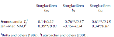
The results show that reconstructed summer temperature serves as a better proxy for b S than the NAO is for b W on annual timescales. In addition, a stronger relationship was found between the tree-ring data and b N than for NAO and b N. On decadal timescales, the relationship between proxies and mass balances changes. There is a strong relationship between NAO and both b W and b N, while the relationship between T S and b S is much weaker than on annual timescales and there is no correlation with b N. This may indicate that the importance of winter and summer climate on b N is timescale-dependent, where the influence on b N of winter accumulation (precipitation) increases, while summer temperatures become less important on decadal timescales. Comparison of the smoothed observed mass-balance records supports this: winter accumulation has more influence on b N (r = 0.93) than summer ablation (r = 0.67) on decadal timescales.
Our approach to reconstructing Storglaciären mass balances was straightforward: we used simple linear regression, with our chosen proxies as predictors, to infer the seasonal and annual mass balance back in time. Since our aim was to reconstruct Storglaciären b N back to 1500, we made several models depending on the relationships found in the correlation analyses. On both annual and decadal timescales, b W and b S were modelled separately and bN was computed by subtracting bS from b W. In addition, both proxies were used together as b N predictors (or a single proxy if a strong relationship was found between that particular proxy and the b N), to model the b N directly. All models were based on linear regression techniques, and the models were initially calibrated using half of the available data, withholding the remaining data for verification. Consequently, 1946–73 was used for calibration and 1974–2000 for verification. The procedure was then reversed, i.e. calibrating the model in 1974–2000 and verifying it in 1946–73. The final models, to reconstruct the Storglaciären b N record back in time, were then based on calibration over the full 1946–2000 period (Table 2).
Table 2. The upper part of the table gives the variance in observed b N explained by the selected predictors as given by regression over two calibration periods. The predictors were summer (June–August) temperatures estimated from tree-ring data (T S; Reference BriffaBriffa and others, 1992) and January–March NAO (Reference LuterbacherLuterbacher and others, 2001). Bold numbers indicate significance at 95% level (only for annual calibrations/verifications). In the lower part, regression equations predicting the net mass balance (b N) of Storglaciären on annual and decadal timescales (decadal values shown in italics) are shown for the full calibration period 1946–2000 (1954–92 decadal), together with the explained variance (r 2)

Results
A total of six estimations of the Storglaciären b N were made, three on each timescale (Table 2). On annual timescales, T S was the dominating predictor, and for that reason all three reconstructions are almost identical regardless of whether or not NAO was included in the model as a predictor. The decadal estimations were largely dependent on NAO as a predictor. However, here there are some differences among the reconstructions, especially between that only based on NAO indices and the others, and for reasons discussed below we chose to focus on the reconstruction based on both NAO and T S data or T S alone. Figure 1 shows reconstructed b N plotted against observed b N on the two timescales. On annual timescales (Fig. 1a), when T S is the most important predictor, all records generally agree well (correlations between observed and reconstructed ranging from 0.61 to 0.68; p = 0.01). The correspondence between reconstructed and observed b N decreases on decadal timescales; disagreements are evident from the mid-1950s to the mid-1970s (Fig. 1b). Looking at the full reconstructions (Fig. 2a), the two reconstructions of the annual b N are almost identical, again indicating that the influence of NAO on b N is very low. On decadal timescales, however, there is a considerable difference between the b N record where b S and b W were reconstructed separately and the record where only NAO was used (Fig. 2b). This is especially conspicuous between the 1740s and 1820s, when the two records are out of phase. The change around 1820 coincides with increased uncertainty in the NAO record; station pressure data from Gibraltar and Reykjavıík were included in the reconstruction from 1820 (Reference LuterbacherLuterbacher and others, 2001). To further evaluate the validity of the reconstructions, b N reconstructions based on both T S and NAO were compared to the Reference Linderholm, Jansson and ChenLinderholm and others (2007) reconstruction of Storglaciären b N (the reconstruction is henceforth referred to as L07) (Fig. 3). L07 was based on more regional proxies (a local tree-ring chronology and circulation indices for northern Scandinavia), and was well correlated (r = 0.8) to the observed b N of Storglaciären. The interannual variabilities of the two reconstructions follow each other well, but the new reconstruction yields slightly higher (more positive) values than L07, except for a few years around 1950. The two reconstructions correspond well on decadal timescales, but again L07 suggests lower b N, especially during the periods ~1830–90 and ~1905–40.

Fig. 1. Observed and modelled (using two different approaches) net mass balances (b N) for Storglaciären: (a) annual resolution; (b) decadal resolution; and (c) scatter plots of the above.

Fig. 2. The full reconstructions of Storglaciären b N based on northern Fennoscandian summer temperatures, reconstructed from tree rings, and the NAO, reconstructed from observed data and documentary sources: (a) annual resolution, and (b) decadal resolution.

Fig. 3. Comparison between the new Storglaciären bN reconstruction and that from Reference Linderholm, Jansson and ChenLinderholm and others (2007) (L07) on both annual and decadal timescales.
The frequency of negative/positive b N years in the last 500 years shows almost equal occurrences of both (53% negative, 47% positive), and there is considerable interannual variability (Fig. 3). Negative b N years dominate the first part of the record, with the two decades 1545–65 being the longest spell of consecutive negative years in the record. From 1570 to 1750, more than two-thirds of the years have positive balances, and b N values increase steadily from 1570 to ~1650, peaking in 1641 with a b N value of 1.72 mw.e. In the following century, positive b N years dominate, but the long-term average is now closer to the zero line. The years with negative b N years between 1751 and 1767 mark a change to a predominantly negative b N phase (63% of the years having negative b N values from 1751 to 2000). However, mass balance becomes progressively more positive in the late 19th and early 20th centuries, peaking in 1902–04 when all three years reach b N > 1.00mw.e. During the 20th century, positive b N years indicate lower net accumulation than earlier in the record, and negative years occasionally reach –1mw.e. or below (the lowest b N year in the record is found in 1937: b N = –1.76mw.e.). On a decadal timescale, the 20th century is very similar to the negative b N period of the 16th century.
Discussion
The large differences in the relationship between mass balance and T S/NAO on different timescales suggest that summer temperatures are more important to mass-balance variability on short timescales, but that the large-scale atmospheric circulation (representing winter accumulation) is more dominant on decadal timescales. However, much of the strong relationship between b N and NAO, on decadal timescales, is based on good correlation from the early 1970s to the present; prior to that it is virtually non-existent (Table 2; Fig. 1b). The nature of this change affects the interpretation of the b N reconstructions back in time that include NAO as a predictor. The change in the influence of the large-scale atmospheric circulations on Storglaciären mass balance since the 1970s corresponds to the NAO having become more pronounced (due to an unusually strong and positive phase). A question that arises is whether the strong relationship between NAO and b N on decadal timescales is an anomaly caused by this unusually strong NAO phase, or whether the lack of correspondence between b N and NAO prior to the 1970s is due to a period of very weak NAO from the mid-1950s to the late 1960s (perhaps the longest negative NAO phase in the last 200 years (e.g. Reference Jacobeit, Jönsson, Bärring, Beck and EkströmJacobeit and others, 2001)). Unfortunately this question is difficult to answer since the Storglaciären mass-balance record starts in 1946. The NAO is more strongly linked to the mass balance of glaciers in southern Norway than those in northern Sweden, mainly due to the progressively decreasing influence on climate of the NAO above 60˚N (Reference Jansson and LinderholmJansson and Linderholm, 2005). Possibly, a large-scale feature like the NAO mainly influences the Storglaciären mass balance during very strong and positive phases (and possibly during single extreme years). If so, we cannot expect that using the NAO as a proxy for high-resolution mass balance of a glacier like Storglaciären will yield realistic results. Previous studies by Reference Pohjola and RogersPohjola and Rogers (1997a), Reference Nordli, Lie, Nesje and BenestadNordli and others (2005) and Reference Linderholm, Jansson and ChenLinderholm and others (2007) have shown that regionally defined circulation indices can be used to provide reasonable estimates of annually resolved winter balances on Scandinavian glaciers, showing that indices on smaller spatial scales than that of the NAO should be preferred.
When NAO and T S are combined to reconstruct Storglaciären b N on annual timescales, the results are identical to those when only T S are used as a predictor. This means that the influence of T S is stronger than that from NAO in the reconstruction, to the extent that it virtually becomes based on T S. This raises the question, to what extent can Storglaciären b N reconstructed from T S be viewed as a good estimate of the actual conditions? Such a scenario requires that b S dominates b N throughout the 500 years. We know that this is not true for the last few decades, when the influence of b W, due to a more maritime climate over Scandinavia, increased. However, Reference Linderholm, Jansson and ChenLinderholm and others (2007) found stronger correlations for (reconstructed) b N = f (b S) than b N = f (b W) between 1781 and 1980, where b S and b W were independently derived and were equally strong proxies of corresponding seasonal mass balance. Furthermore, when compared, the present b N reconstruction and L07 are in good agreement (Fig. 3) (b N(TS) vs L07: r = 0.78, p = 0.01; b N(TS+NAO) vs L07: r = 0.80, p = 0.01). Also the decadal evolutions of the reconstructions shown in Figure 3 are well correlated, although b N based on T S is better correlated to L07 (r = 0.82) than b N based on T S and NAO (r = 0.71). This may be surprising when the correlation between b N and T S is low over the full 1954–92 period. However, Table 2 shows that when the correlation is computed in the two subgroups, it is almost as strong as that for NAO. The reason for this is a change in the sign of the correlation in the late 1970s, where T S is negatively correlated to b N before 1980 but positively correlated thereafter. We may assume that the T S-based reconstruction of Storglaciären bN provides a good estimate of the actual conditions back to AD 1500, but it is likely that the reconstruction is biased during years or periods of increased (positive) NAO strength provided that conditions have been similar to those of the last few decades. If so, it is likely that T S underestimates b N.
The cumulative b N from a number of reconstructions (Fig. 4) on both timescales suggests that the b N values in the late 16th century were as low as those of the late 20th century. The b N then steadily increases to a maximum around 1750, which falls into the period (17th century and beginning of 18th century) when glaciers in Sweden probably reached their greatest Holocene extent (Karlen, 1988). This is followed by a general decrease that continues until today, but the b N variability between 1750 and 1900 is higher than in other periods. The decrease is punctuated by periods of increasing b N, which may correspond to inferred glacier advances (e.g. 1780, 1800–10; Reference KarlénKarlén, 1988). Our new b N reconstruction better supports glacier build-up and expansion in the late 19th century and early 20th century, when the post-18th-century maximum of Storglaciären was reached (Reference HolmlundHolmlund, 1987), compared to L07.

Fig. 4. Cumulative reconstructed and observed b N for Storglaciären. For easier comparison, they have been scaled to a zero mass balance in 1946 (when actual observations began).
From Figure 4 it is clear that all reconstructions overestimate the observed b N during most of the calibration period of the models, so it is very likely that the reconstructed b N prior to 1946 also are overestimated. Furthermore, when our (smoothed) b N reconstructions are compared to a reconstruction of Storglaciären volume back to AD 500 by Reference Raper, Briffa and WigleyRaper and others (1996) (Fig. 5), our reconstructions (and especially L07) provide much less variability between 1750 and 1900. Still, there is a large measure of agreement between our records and those of Raper and others, mainly because they also used the tree-ring-based reconstruction of Fennoscandian summer temperatures by Reference BriffaBriffa and others (1992) as a forcing of their model. One of the limitations in Reference Raper, Briffa and WigleyRaper and others’ (1996) volume reconstruction was that, due to lack of long-term accumulation data, they could only reconstruct the summer-temperature-dependent part of the volume changes (e.g. see their fig 5b, where the volume is overestimated). The closest agreement we obtained with observed b N values on decadal timescales was provided when using both T S and NAO, so it is likely that inclusion of proxies for both winter and summer balances (despite the records being large-scale) will provide better estimates than using only the summer part of the mass balance when attempting to reconstruct the net balance.

Fig. 5. Cumulative mass balances (decadal) from this work and L07 compared to a reconstruction of Storglaciären volume from Reference Raper, Briffa and WigleyRaper and others (1996). The curves have been adjusted to roughly correspond to the observed values of Storglaciären volume at the end of the record.
It is surprising that the b N record (L07), which is the best estimate of interannual variability in the observed record (r = 0.8), displayed an unrealistic b N evolution (cumulative).
This is probably due to the lack of low-frequency variability in the data used to infer the winter balance (regional circulation indices; see Reference LuterbacherLinderholm and others, 2007). Thus, the next step to provide a better reconstruction of Storglaciären mass balance, to be used to attempt to improve the model of past volume changes, is to devise a long, regional circulation index with variability on short to long timescales.
Conclusion
We show that regional summer temperatures (here reconstructed from tree-ring data) can be used to infer past changes in both summer and net balance of Storglaciären on an annual timescale. On decadal timescales, the relationship was much weaker. The opposite was true for winter NAO as a proxy for winter and net balance. A strong link was found between NAO and net balance on decadal timescales, suggesting that on longer timescales winter accumulation (as a function of large-scale atmospheric circulation) increases its influence on the net balance. However, this feature may depend on an unusually strong and positive phase of the NAO in the 1980s and 1990s. The winter NAO possibly influences the net balance in unusually strong positive phases or single years; otherwise summer temperatures (representing summer ablation) are more important for the net balance of a glacier of the Storglaciären type. Despite the uncertainties regarding the influence of winter balance, we suggest that a reconstruction based on summer temperatures can provide an acceptable estimate of past net balance variability. The Storglaciären net balance reconstructed back to AD 1500 with annual resolution agrees well with previous (shorter) reconstructions but also with other evidence of glacier fluctuations (historical, geomorphological, etc.). However, to better understand the influence and variability of the winter accumulation on the net balance, efforts should be made to extend regional–local proxies (e.g. atmospheric circulation indices).
Acknowledgements
We acknowledge K. Briffa for providing the Fennoscandian temperature reconstruction and J. Luterbacher for providing the NAO data used in this study. This research was supported by the Swedish Research Council (VR, grant to H. Linderholm). The comments from two anonymous reviewers helped sharpen the manuscript.


