





1. Introduction
The actuator disk model is one of the most fundamental models in fluid dynamics for analysing turbine rotors and propellers (van Kuik Reference van Kuik2022). First proposed by Rankine and later refined into its classical form by Froude in 1889 (Okulov & Van Kuik Reference Okulov and Van Kuik2012), it is now commonly referred to as Froude’s actuator disk theory. The model represents the complex loading of a rotor as a simple pressure jump across an infinitely thin, permeable disk of the same diameter, known as an actuator disk. Despite its simplicity, the theory remains a cornerstone of rotor fluid dynamics because it provides clear and intuitive insights into rotor performance. Froude’s actuator disk theory is typically one of the very first conceptual models introduced to students and researchers interested in the fluid mechanics of turbomachinery. It appears in almost every major wind energy textbook (e.g. Burton et al. Reference Burton, Sharpe, Jenkins and Bossanyi1995; Spera Reference Spera2009; Manwell, McGowan & Rogers Reference Manwell, McGowan and Rogers2010; Hansen Reference Hansen2015; Sørensen Reference Sørensen2016; Branlard Reference Branlard2017, among others), and classical aerodynamics and hydrodynamic textbooks on propellers and rotors (e.g. Breslin & Andersen Reference Breslin and Andersen1994; Leishman Reference Leishman2006; Seddon & Newman Reference Seddon and Newman2011; Carlton Reference Carlton2018, among others).
Despite its historical importance and value as a simple conceptual model, Froude’s theory has important limitations. First, it does not describe how flow variables evolve with streamwise distance and only relates conditions far upstream and far downstream to those on the actuator disk. Second, the model does not describe the turbulent wake behaviour since the predicted downstream velocity asymptotes to $U_0 (1 - 2a)$
, where
$U_0 (1 - 2a)$
, where $U_0$
is the incoming velocity and
$U_0$
is the incoming velocity and $a$
is the induction factor, and the wake width becomes constant after an initial expansion. In reality, following the initial velocity reduction due to pressure recovery, the wake gradually recovers through turbulent mixing, and wake expansion continues downstream. For these reasons, Froude’s theory is generally regarded as conceptually relevant only in the region immediately downstream of the disk, before turbulence dominates.
$a$
is the induction factor, and the wake width becomes constant after an initial expansion. In reality, following the initial velocity reduction due to pressure recovery, the wake gradually recovers through turbulent mixing, and wake expansion continues downstream. For these reasons, Froude’s theory is generally regarded as conceptually relevant only in the region immediately downstream of the disk, before turbulence dominates.
The limitations become especially severe for highly loaded actuator disks (with induction factors $a \gt 0.5$
), where the model even predicts negative wake velocities. Likewise, the well-known relation for the thrust coefficient
$a \gt 0.5$
), where the model even predicts negative wake velocities. Likewise, the well-known relation for the thrust coefficient $C_T = 4a(1-a)$
breaks down in this regime and fails to provide meaningful results (Manwell et al. Reference Manwell, McGowan and Rogers2010). This breakdown is believed to result from strong shear that drives the wake into a fully turbulent state and promotes strong interactions with the ambient flow, effects absent from Froude’s formulation. To mitigate these limitations, empirical corrections are often introduced to adjust the
$C_T = 4a(1-a)$
breaks down in this regime and fails to provide meaningful results (Manwell et al. Reference Manwell, McGowan and Rogers2010). This breakdown is believed to result from strong shear that drives the wake into a fully turbulent state and promotes strong interactions with the ambient flow, effects absent from Froude’s formulation. To mitigate these limitations, empirical corrections are often introduced to adjust the $C_T$
–
$C_T$
– $a$
relationship (Burton et al. Reference Burton, Sharpe, Jenkins and Bossanyi1995; Buhl Reference Buhl2005). For a highly loaded actuator disk (i.e. a disk with low porosity), where a significant portion of the fluid bypasses the disk rather than passing through it, the actuator disk behaves more like a solid plate. In this case, intense wake turbulence and flow separation generate a strong negative pressure behind the disk, contributing to pressure drag (Roshko Reference Roshko1955). Steiros & Hultmark (Reference Steiros and Hultmark2018) accounted for this negative wake pressure by formulating governing equations for a control volume (CV) surrounding the disk that has non-zero pressure at the outlet, unlike Froude’s original formulation. The flow inside the CV is assumed to be inviscid and irrotational, and the outlet is placed immediately before the region where turbulent mixing becomes significant. However, because introducing a non-zero outlet pressure adds an extra unknown, additional information is needed to close the system of equations. To address this, they modelled the actuator disk using potential flow theory. As representing the disk as a distribution of potential sources results in an unrealistic velocity discontinuity at the disk plane, they rescaled the wake velocities to enforce mass conservation and validated their predictions against water-channel experiments of porous flat plates. More recently, Liew, Heck & Howland (Reference Liew, Heck and Howland2024) adopted a similar CV analysis, but determined the negative pressure at the CV outlet by solving the two-dimensional pressure Poisson equation proposed by Madsen (Reference Madsen2023). They assumed that the CV outlet coincides with the end of the near wake, whose length was estimated using the method of Bastankhah & Porté-Agel (Reference Bastankhah and Porté-Agel2016). They also extended this framework to yawed rotors to predict a
$a$
relationship (Burton et al. Reference Burton, Sharpe, Jenkins and Bossanyi1995; Buhl Reference Buhl2005). For a highly loaded actuator disk (i.e. a disk with low porosity), where a significant portion of the fluid bypasses the disk rather than passing through it, the actuator disk behaves more like a solid plate. In this case, intense wake turbulence and flow separation generate a strong negative pressure behind the disk, contributing to pressure drag (Roshko Reference Roshko1955). Steiros & Hultmark (Reference Steiros and Hultmark2018) accounted for this negative wake pressure by formulating governing equations for a control volume (CV) surrounding the disk that has non-zero pressure at the outlet, unlike Froude’s original formulation. The flow inside the CV is assumed to be inviscid and irrotational, and the outlet is placed immediately before the region where turbulent mixing becomes significant. However, because introducing a non-zero outlet pressure adds an extra unknown, additional information is needed to close the system of equations. To address this, they modelled the actuator disk using potential flow theory. As representing the disk as a distribution of potential sources results in an unrealistic velocity discontinuity at the disk plane, they rescaled the wake velocities to enforce mass conservation and validated their predictions against water-channel experiments of porous flat plates. More recently, Liew, Heck & Howland (Reference Liew, Heck and Howland2024) adopted a similar CV analysis, but determined the negative pressure at the CV outlet by solving the two-dimensional pressure Poisson equation proposed by Madsen (Reference Madsen2023). They assumed that the CV outlet coincides with the end of the near wake, whose length was estimated using the method of Bastankhah & Porté-Agel (Reference Bastankhah and Porté-Agel2016). They also extended this framework to yawed rotors to predict a $C_T$
–
$C_T$
– $a$
relationship that shows good agreement with large-eddy simulation (LES) data for various cases. While these approaches provide improved predictions for highly loaded disks, they still do not overcome the important limitation of Froude’s actuator disk theory; namely, its inability to incorporate effects of turbulent mixing induced by strong velocity shear that may occur in the immediate downstream vicinity of a highly loaded disk.
$a$
relationship that shows good agreement with large-eddy simulation (LES) data for various cases. While these approaches provide improved predictions for highly loaded disks, they still do not overcome the important limitation of Froude’s actuator disk theory; namely, its inability to incorporate effects of turbulent mixing induced by strong velocity shear that may occur in the immediate downstream vicinity of a highly loaded disk.
Turbulent wake development is more realistically represented in far-wake analytical models, which are widely used in wind energy applications to characterise wake interactions in wind farms (see reviews by Stevens & Meneveau Reference Stevens and Meneveau2017; Porté-Agel et al. Reference Porté-Agel, Bastankhah and Shamsoddin2020, and references therein). These models are generally based on momentum theory, where pressure effects are neglected under the far-wake assumption, so that the thrust force balances the streamwise flux of momentum deficit (Bastankhah & Porté-Agel Reference Bastankhah and Porté-Agel2014). Although recent wake models aim to use more realistic velocity profiles in the near wake (e.g. Shapiro et al. Reference Shapiro, Starke, Meneveau and Gayme2019; Blondel & Cathelain Reference Blondel and Cathelain2020; Schreiber, Balbaa & Bottasso Reference Schreiber, Balbaa and Bottasso2020; Ali, Stallard & Ouro Reference Ali, Stallard and Ouro2024, among others), their neglect of pressure effects prevents them from accurately capturing the flow immediately behind the disk, where such effects remain significant. Consequently, analytical wake models typically require assumptions about near-wake conditions as inputs. Examples include specifying the onset of the far-wake region, the initial wake width or the downstream location where the velocity deficit reaches its maximum. Moreover, commonly used far-wake models typically fail to provide reliable predictions for induction factors $a \gt 0.25$
in the far-wake region (Bempedelis & Steiros Reference Bempedelis and Steiros2022). For instance, the widely used top-hat model of Frandsen et al. (Reference Frandsen, Barthelmie, Pryor, Rathmann, Larsen, Højstrup and Thøgersen2006) and the Gaussian model of Bastankhah & Porté-Agel (Reference Bastankhah and Porté-Agel2014) may predict a decrease in the maximum wake velocity deficit as the induction factor
$a \gt 0.25$
in the far-wake region (Bempedelis & Steiros Reference Bempedelis and Steiros2022). For instance, the widely used top-hat model of Frandsen et al. (Reference Frandsen, Barthelmie, Pryor, Rathmann, Larsen, Højstrup and Thøgersen2006) and the Gaussian model of Bastankhah & Porté-Agel (Reference Bastankhah and Porté-Agel2014) may predict a decrease in the maximum wake velocity deficit as the induction factor $a$
increases beyond 0.25 (i.e.
$a$
increases beyond 0.25 (i.e. $C_T \gt 0.75$
), which is not physically expected. Although more recent studies (e.g. Bempedelis & Steiros Reference Bempedelis and Steiros2022) have incorporated pressure effects into the far-wake evolution of highly loaded disks, they remain limited to the far-wake region, where velocity monotonically increases with streamwise distance from the disk. This behaviour is not valid in the region immediately behind the disk.
$C_T \gt 0.75$
), which is not physically expected. Although more recent studies (e.g. Bempedelis & Steiros Reference Bempedelis and Steiros2022) have incorporated pressure effects into the far-wake evolution of highly loaded disks, they remain limited to the far-wake region, where velocity monotonically increases with streamwise distance from the disk. This behaviour is not valid in the region immediately behind the disk.
This paper aims to bridge the gap between two traditionally separate areas of research, actuator disk theory and turbulent wakes. We show that it is possible to overcome the limitations outlined earlier by developing a new actuator disk theory that includes wake recovery due to turbulent entrainment. While still idealised, the proposed approach provides a more accurate and physically meaningful representation of actuator-disk flows.
2. Generalised actuator disk theory including wake development
We consider the ‘hybrid’ CV around a disk, as shown in figure 1. Upwind of the disk, as in Froude’s theory, we assume there is no mass exchange between the CV and the surroundings, so the CV is the streamtube encompassing the rotor disk. This assumption implies that turbulent mixing does not play a significant role in shaping the flow distribution upstream of the disk. This notion is supported by previous studies showing that inviscid solutions often provide satisfactory predictions in this region (e.g. Medici et al. Reference Medici, Ivanell, Dahlberg and Alfredsson2011; Bastankhah & Porté-Agel Reference Bastankhah and Porté-Agel2017; Segalini Reference Segalini2021). Downstream of the rotor disk, however, the CV is not a streamtube, but is assumed to coincide with the outer boundary of the wake, where turbulence drives entrainment of the ambient flow through the lateral surface of the CV, until the wake is fully recovered. For this CV, at each streamwise position $x$
, the velocity
$x$
, the velocity $U(x)$
and pressure
$U(x)$
and pressure $P(x)$
are assumed to be uniform, with the diameter of the CV cross-section denoted by
$P(x)$
are assumed to be uniform, with the diameter of the CV cross-section denoted by $\sigma (x)$
. The disk is located at
$\sigma (x)$
. The disk is located at $x=0$
and the diameter of the CV at
$x=0$
and the diameter of the CV at $x=0$
is equal to the disk diameter
$x=0$
is equal to the disk diameter $D$
. Subscripts
$D$
. Subscripts $0$
and
$0$
and $\infty$
denote the asymptotic far-upstream (
$\infty$
denote the asymptotic far-upstream ( $x\!\to \!-\infty$
) and far-downstream (
$x\!\to \!-\infty$
) and far-downstream ( $x\!\to \!\infty$
) values, respectively.
$x\!\to \!\infty$
) values, respectively.
In Froude’s original formulation, the CV extends from far upstream to far downstream. Here, to capture the streamwise variations of the flow quantities, we retain the inlet at far upstream, but place the CV outlet at an arbitrary streamwise location $x$
, where
$x$
, where $x$
can take on positive or negative values. The goal of our analysis is to determine
$x$
can take on positive or negative values. The goal of our analysis is to determine $P(x)$
,
$P(x)$
, $U(x)$
,
$U(x)$
, $\sigma (x)$
and thrust coefficient
$\sigma (x)$
and thrust coefficient $C_T$
for a given induction factor
$C_T$
for a given induction factor $a$
(or for a known
$a$
(or for a known $C_T$
, to determine
$C_T$
, to determine $a$
).
$a$
).
Schematic of the control volume (CV) used in the new proposed actuator disk theory. The upstream part of the CV is a streamtube, while the downstream part follows the wake borders and therefore there is flow entrainment from the lateral area. The outlet is at an arbitrary downstream location with a diameter of $\sigma (x)$
, pressure
$\sigma (x)$
, pressure $P=P(x)$
and velocity
$P=P(x)$
and velocity $U=U(x)$
. The disk is located at
$U=U(x)$
. The disk is located at $x=0$
.
$x=0$
.

2.1. Mass conservation
The conservation of mass for this CV is written as
 \begin{equation} \dot {m}(x)=\dot {m}_0+\dot {m}_e(x), \end{equation}
where $\dot {m}_0=({\pi }/{4}) \rho \sigma ^2_0 U_0$
and
$\dot {m}_0=({\pi }/{4}) \rho \sigma ^2_0 U_0$
and $\dot {m}(x)=({\pi }/{4}) \rho \sigma ^2(x) U(x)$
are the mass flow rates at the inlet and outlet, respectively, and
$\dot {m}(x)=({\pi }/{4}) \rho \sigma ^2(x) U(x)$
are the mass flow rates at the inlet and outlet, respectively, and $\dot {m}_e(x)$
represents the mass flow rate of the entrained flow across the lateral surface. Also,
$\dot {m}_e(x)$
represents the mass flow rate of the entrained flow across the lateral surface. Also, $\rho$
is the air density. If we define the entrainment velocity as
$\rho$
is the air density. If we define the entrainment velocity as $U_e(x)$
, the axial rate of change of
$U_e(x)$
, the axial rate of change of $\dot {m}_e(x)$
can be written as the product of perimeter times entrainment velocity and is given by
$\dot {m}_e(x)$
can be written as the product of perimeter times entrainment velocity and is given by
 \begin{equation} \frac {\mathrm{d}\dot {m}_e}{\mathrm{d}x}=\rho \pi \,\sigma (x) \, U_e(x) \, \mathrm{H}(x), \end{equation}
where $\mathrm{H}(x)$
is the Heaviside function, which ensures that the entrainment driven by turbulence only takes place downwind of the actuator disk. Taking the derivative of (2.1) with respect to
$\mathrm{H}(x)$
is the Heaviside function, which ensures that the entrainment driven by turbulence only takes place downwind of the actuator disk. Taking the derivative of (2.1) with respect to $x$
and using (2.2), we obtain
$x$
and using (2.2), we obtain
 \begin{equation} \frac {\mathrm{d}\big (\sigma ^2 U\big )}{\mathrm{d}x}=4\sigma U_e\mathrm{H}(x), \end{equation}
which can be expanded and rearranged as
 \begin{equation} \frac {\mathrm{d}\sigma }{\mathrm{d}x} = \frac {1}{2U} \left (\! - \sigma \frac {\mathrm{d}U}{\mathrm{d}x} + 4U_e\mathrm{H}(x)\right )\!. \end{equation}
2.2. Choice of entrainment velocity $U_e$
$U_e$

2.2.1. Wake-shear driven entrainment
In the absence of ambient turbulence, turbulent entrainment is primarily driven by wake shear. In studies applying entrainment theory to wake flows (Morton Reference Morton1961; Luzzatto-Fegiz Reference Luzzatto-Fegiz2018; Luzzatto-Fegiz & Caulfield Reference Luzzatto-Fegiz and Caulfield2018; Bempedelis & Steiros Reference Bempedelis and Steiros2022; Bempedelis, Laizet & Deskos Reference Bempedelis, Laizet and Deskos2023), the entrainment rate is typically modelled as a function of the characteristic velocity difference, so the entrainment velocity is modelled as
 \begin{equation} \frac {U_e^w(x)}{U_0} = E_1 \frac {\Delta U(x)}{U_0}, \end{equation}
where $\Delta U(x) = U_0 - U(x)$
represents the velocity deficit, the superscript
$\Delta U(x) = U_0 - U(x)$
represents the velocity deficit, the superscript $w$
denotes wake-shear driven entrainment and the parameter
$w$
denotes wake-shear driven entrainment and the parameter $E_1$
is the shear-driven entrainment coefficient. Here, we assume
$E_1$
is the shear-driven entrainment coefficient. Here, we assume $E_1 = 0.1$
, consistent with classical entrainment studies (Morton Reference Morton1961).
$E_1 = 0.1$
, consistent with classical entrainment studies (Morton Reference Morton1961).
2.2.2. Background-turbulence-driven entrainment
In addition to wake shear, background turbulence also plays a significant role in the entrainment process and wake evolution. This is particularly relevant for cases where the actuator disk (e.g. a wind turbine) operates in a deep atmospheric boundary layer that contains large-scale energetic eddies. These eddies typically have a cross-stream length scale comparable to the height from the ground, and often a streamwise length considerably larger than the wake width $\sigma$
, scaling closer to the overall boundary layer thickness. We denote their overall size by an integral length scale
$\sigma$
, scaling closer to the overall boundary layer thickness. We denote their overall size by an integral length scale $\varLambda$
in this work. Under these conditions, the wake is transported and meandered by the incoming large-scale turbulent eddies (Larsen et al. Reference Larsen, Madsen, Thomsen and Larsen2008). Therefore, the entrainment velocity in this regime is determined primarily by the inflow characteristics. We assume that the entrainment velocity driven by background turbulence is proportional to the root-mean-square of the incoming streamwise velocity fluctuations. When normalised by the incoming velocity
$\varLambda$
in this work. Under these conditions, the wake is transported and meandered by the incoming large-scale turbulent eddies (Larsen et al. Reference Larsen, Madsen, Thomsen and Larsen2008). Therefore, the entrainment velocity in this regime is determined primarily by the inflow characteristics. We assume that the entrainment velocity driven by background turbulence is proportional to the root-mean-square of the incoming streamwise velocity fluctuations. When normalised by the incoming velocity $U_0$
, this implies that the normalised entrainment velocity is proportional to the streamwise turbulence intensity
$U_0$
, this implies that the normalised entrainment velocity is proportional to the streamwise turbulence intensity $I$
. It is worth noting that the dependency of the entrainment velocity on the integral length scale
$I$
. It is worth noting that the dependency of the entrainment velocity on the integral length scale $\varLambda$
is neglected here for simplicity, which may not be completely true (Hodgson, Madsen & Andersen Reference Hodgson, Madsen and Andersen2023; Li et al. Reference Li, Zhang, Li and Yang2024; Vahidi & Porté-Agel Reference Vahidi and Porté-Agel2024). We further note that the turbulence intensity can be defined based on either the total turbulent kinetic energy or its streamwise component alone. While the former may be more physically grounded, the latter is easier to measure and is the standard definition used in most current wind energy research (Porté-Agel et al. Reference Porté-Agel, Bastankhah and Shamsoddin2020). There is a subtle point regarding the onset of entrainment due to background turbulence that also needs to be discussed. Previous studies (e.g. Lignarolo et al. Reference Lignarolo, Ragni, Scarano, Ferreira and Van Bussel2015) have demonstrated that the strong vortex layer surrounding the near wake inhibits interaction with the ambient flow. To capture this shielding effect, we link the entrainment contribution from background turbulence to the degree of pressure recovery downstream of the wake. This implies that the entrainment due to background turbulence is effectively suppressed at
$\varLambda$
is neglected here for simplicity, which may not be completely true (Hodgson, Madsen & Andersen Reference Hodgson, Madsen and Andersen2023; Li et al. Reference Li, Zhang, Li and Yang2024; Vahidi & Porté-Agel Reference Vahidi and Porté-Agel2024). We further note that the turbulence intensity can be defined based on either the total turbulent kinetic energy or its streamwise component alone. While the former may be more physically grounded, the latter is easier to measure and is the standard definition used in most current wind energy research (Porté-Agel et al. Reference Porté-Agel, Bastankhah and Shamsoddin2020). There is a subtle point regarding the onset of entrainment due to background turbulence that also needs to be discussed. Previous studies (e.g. Lignarolo et al. Reference Lignarolo, Ragni, Scarano, Ferreira and Van Bussel2015) have demonstrated that the strong vortex layer surrounding the near wake inhibits interaction with the ambient flow. To capture this shielding effect, we link the entrainment contribution from background turbulence to the degree of pressure recovery downstream of the wake. This implies that the entrainment due to background turbulence is effectively suppressed at $x=0$
and asymptotically approaches its maximum value as the wake pressure recovers. Inspired by the pressure variation downstream of the actuator disk derived later in § 2.4 (2.14), we propose the following relation:
$x=0$
and asymptotically approaches its maximum value as the wake pressure recovers. Inspired by the pressure variation downstream of the actuator disk derived later in § 2.4 (2.14), we propose the following relation:
 \begin{equation} \frac {U_e^{b}}{U_0} = E_2 I \frac {x}{\sqrt {x^2+R^2}}, \end{equation}
where $E_2$
is the background-driven entrainment coefficient, superscript
$E_2$
is the background-driven entrainment coefficient, superscript $b$
stands for background turbulence and
$b$
stands for background turbulence and $R=D/2$
is the rotor radius. It will be shown later in § 3.2.2 that
$R=D/2$
is the rotor radius. It will be shown later in § 3.2.2 that $E_2$
is expected to be in the range of
$E_2$
is expected to be in the range of $[0.25{-}1]$
. In this study, we use the value
$[0.25{-}1]$
. In this study, we use the value $E_2=0.6$
as it provides reasonable agreement with experimental and LES data presented later in § 3.3.
$E_2=0.6$
as it provides reasonable agreement with experimental and LES data presented later in § 3.3.
2.2.3. Total entrainment driven by wake shear and background turbulence
We propose that the total entrainment velocity is proportional to the generalised mean of the normalised velocity deficit and the incoming turbulence intensity:
 \begin{equation} \frac {U_e(x)}{U_0} = \left [ \left ( \frac {U_e^w}{U_0}\right )^n + \left ( \frac {U_e^{b}}{U_0} \right )^n \right ]^{1/n}\!, \end{equation}
where $n$
is a positive integer. Here, we assume
$n$
is a positive integer. Here, we assume $n=4$
, noting that larger values do not lead to a considerable difference. The advantage of using (2.7) is that the entrainment velocity closely approaches the larger of the two contributing factors. Consequently, under typical conditions, the near-wake entrainment velocity is dominated by the wake shear, which is generally larger in that region, while in the far wake, the entrainment velocity is dominated by background turbulence.
$n=4$
, noting that larger values do not lead to a considerable difference. The advantage of using (2.7) is that the entrainment velocity closely approaches the larger of the two contributing factors. Consequently, under typical conditions, the near-wake entrainment velocity is dominated by the wake shear, which is generally larger in that region, while in the far wake, the entrainment velocity is dominated by background turbulence.
2.3. Momentum balance
The momentum equation for the CV shown in figure 1 is given by
 \begin{equation} \rho \frac {\pi }{4}\sigma ^{2}(x)\, U(x) \, [U_{0}-U(x)] =\rho \frac {\pi }{8} C_{T}U_{0}^{2} D^{2} \mathrm{H}(x)+\frac {\pi }{4}\sigma ^{2}(x) P(x) -F_{\!P_s}(x), \end{equation}
where the momentum deficit flux term on the left-hand-side is written using the mass conservation (2.1), i.e. $\dot {m}_e=({\pi }/{4}) \rho (\sigma ^2 U- \sigma ^2_0 U_0)$
and its associated momentum flux
$\dot {m}_e=({\pi }/{4}) \rho (\sigma ^2 U- \sigma ^2_0 U_0)$
and its associated momentum flux $\dot {m}_e U_0$
. In (2.8), the term
$\dot {m}_e U_0$
. In (2.8), the term $F_{\!P_s}(x)$
is the axial component of the force exerted by the pressure on the lateral surface of the streamtube, given by
$F_{\!P_s}(x)$
is the axial component of the force exerted by the pressure on the lateral surface of the streamtube, given by
 \begin{equation} F_{\!P_s}(x)= \frac {\pi }{4}\int _{-\infty }^{x}P(x') \, \frac {{\,\mathrm{d}} \sigma ^2(x')}{{\,\mathrm{d}} x'} {\,\mathrm{d}} x', \end{equation}
where $x'$
is a dummy variable. Equation (2.9) is obtained by integrating the pressure force exerted on an infinitesimal lateral area, shown in figure 2(a), from far upstream to
$x'$
is a dummy variable. Equation (2.9) is obtained by integrating the pressure force exerted on an infinitesimal lateral area, shown in figure 2(a), from far upstream to $x$
. In Froude’s actuator theory, the lateral pressure term is neglected because the CV’s outlet is assumed to be sufficiently far downstream, such that the lateral pressure force contribution downstream cancels that upstream, resulting in a net effect of zero. This zero net contribution in the far wake can be understood by considering a spherical control volume of very large radius,
$x$
. In Froude’s actuator theory, the lateral pressure term is neglected because the CV’s outlet is assumed to be sufficiently far downstream, such that the lateral pressure force contribution downstream cancels that upstream, resulting in a net effect of zero. This zero net contribution in the far wake can be understood by considering a spherical control volume of very large radius, $R_s\!\to \! \infty$
, surrounding the disk, as shown in figure 2(b). For this CV, the lateral pressure forces are all internal (van Kuik Reference van Kuik2022) and the pressure at the control surface is atmospheric everywhere. Consequently, (2.8) reduces to a simple balance between the thrust force and the net momentum flux across the control surface. However, it is important to note that for a finite
$R_s\!\to \! \infty$
, surrounding the disk, as shown in figure 2(b). For this CV, the lateral pressure forces are all internal (van Kuik Reference van Kuik2022) and the pressure at the control surface is atmospheric everywhere. Consequently, (2.8) reduces to a simple balance between the thrust force and the net momentum flux across the control surface. However, it is important to note that for a finite $x$
(either positive or negative) considered here, the net contribution of the lateral pressure term is non-zero and must be retained in the momentum equation.
$x$
(either positive or negative) considered here, the net contribution of the lateral pressure term is non-zero and must be retained in the momentum equation.
(a) Pressure force exerted on an infinitesimal lateral area. (b) Schematic of a spherical CV with an infinitely large radius surrounding the disk. For this CV, unlike the one shown in figure 1 that is used in our present model formulation, lateral pressure forces are internal forces and do not appear in the momentum equation.

Taking the derivative of (2.8) with respect to $x$
and rearranging terms leads to
$x$
and rearranging terms leads to
 \begin{equation} U\frac {\mathrm{d}U}{\mathrm{d}x}+ \frac {1}{\rho }\frac {\mathrm{d}P}{\mathrm{d}x}=\left (\frac {2U}{\sigma }\frac {\mathrm{d}\sigma }{\mathrm{d}x}+\frac {\mathrm{d}U}{\mathrm{d}x}\right )(U_0-U)-\frac {1}{2} C_{T}U_{0}^{2} \mathrm{\delta }(x), \end{equation}
where $\delta (x)$
is the Dirac delta function. Using (2.4) to express
$\delta (x)$
is the Dirac delta function. Using (2.4) to express ${\mathrm{d}}\sigma /{\,\mathrm{d}} x$
allows (2.10) to be written as
${\mathrm{d}}\sigma /{\,\mathrm{d}} x$
allows (2.10) to be written as
 \begin{equation} U(x)\frac {\mathrm{d}U}{\mathrm{d}x}+ \frac {1}{\rho }\frac {\mathrm{d}P}{\mathrm{d}x}=-\frac {1}{2} C_{T}U_{0}^{2} \mathrm{\delta }(x) + \frac {4U_e(x)[U_0-U(x)]\, \mathrm{H}(x)}{\sigma (x)}. \end{equation}
It is worth noting that (2.11) bears a strong resemblance to the differential Reynolds-averaged Navier–Stokes (RANS) equation in the $x$
-direction, provided the Reynolds shear stress term is simplified using scaling arguments (i.e. replacing radial gradients with variations over wake radius
$x$
-direction, provided the Reynolds shear stress term is simplified using scaling arguments (i.e. replacing radial gradients with variations over wake radius $\sigma /2$
). This comparison also suggests that
$\sigma /2$
). This comparison also suggests that $U_e\sigma$
essentially acts as an effective turbulent viscosity. Integrating (2.11) from
$U_e\sigma$
essentially acts as an effective turbulent viscosity. Integrating (2.11) from $-\infty$
to
$-\infty$
to $x$
results in the following Bernoulli-type equation:
$x$
results in the following Bernoulli-type equation:
 \begin{align} \frac {1}{\rho }\,P(x)+\frac {1}{2}U^2(x)=\frac {1}{2}U_0^2\left (1- C_T \mathrm{H}(x) \right )+ 4 \int _0^{\textit{max}(x,0)} \frac {U_e(x')\,[U_0-U(x')]}{\sigma (x')} \, \mathrm{d}x', \end{align}
which represents the variation of the mechanical energy with $x$
. It can also be regarded as a generalised form of the Bernoulli equation, with two additional effects incorporated: the extraction of energy by the disk (i.e. the
$x$
. It can also be regarded as a generalised form of the Bernoulli equation, with two additional effects incorporated: the extraction of energy by the disk (i.e. the $-C_T\mathrm{H}(x)$
term on the right-hand side) and the entrainment of energy by turbulence (the last term on the right-hand side). When
$-C_T\mathrm{H}(x)$
term on the right-hand side) and the entrainment of energy by turbulence (the last term on the right-hand side). When $C_T=U_e = 0$
, this equation reduces to a Bernoulli equation. It is also important to note that the derivation of this generalised form of the Bernoulli equation from mass and momentum equations is possible when the momentum equation is written in its complete form including the lateral pressure term
$C_T=U_e = 0$
, this equation reduces to a Bernoulli equation. It is also important to note that the derivation of this generalised form of the Bernoulli equation from mass and momentum equations is possible when the momentum equation is written in its complete form including the lateral pressure term $F_{\!P_s}$
.
$F_{\!P_s}$
.
Finally, (2.11) can be rearranged as
 \begin{equation} \frac {\mathrm{d}U}{\mathrm{d}x} = \frac {1}{U} \left (\! -\frac {1}{\rho } \frac {\mathrm{d}P}{\mathrm{d}x} - \frac {1}{2} C_{T} U_0^2\, \delta (x) + \frac {4U_e(U_0 - U)\, \mathrm{H}(x)}{\sigma } \right )\!. \end{equation}
We then have a system of two ordinary differential equations comprising (2.13) for $\mathrm{d}U/\mathrm{d}x$
and (2.4) for
$\mathrm{d}U/\mathrm{d}x$
and (2.4) for $\mathrm{d}\sigma /\mathrm{d}x$
. However, there are three dependent variables,
$\mathrm{d}\sigma /\mathrm{d}x$
. However, there are three dependent variables, $U(x)$
,
$U(x)$
, $\sigma (x)$
and
$\sigma (x)$
and $P(x)$
, with
$P(x)$
, with $x$
as the independent variable. The required third equation (for
$x$
as the independent variable. The required third equation (for $\mathrm{d}P/\mathrm{d}x$
) is obtained in the next section.
$\mathrm{d}P/\mathrm{d}x$
) is obtained in the next section.
2.4. Pressure variations for lightly loaded actuator disks
Here, we aim to solve a simplified form of the pressure Poisson equation to determine $P(x)$
. Previous studies have solved the linearised pressure Poisson equation over the entire domain (
$P(x)$
. Previous studies have solved the linearised pressure Poisson equation over the entire domain ( $-\infty \! \lt \! x\! \lt \! \infty$
) that includes actuator-disk forcing using three-dimensional (3-D) axisymmetric (Koning Reference Koning1935; Segalini Reference Segalini2021) and two-dimensional (2-D) Cartesian (Madsen Reference Madsen2023; Liew et al. Reference Liew, Heck and Howland2024) formulations, although 2-D approaches are inherently less realistic for 3-D rotors. Since linearised solutions neglect nonlinear terms in the pressure Poisson equation, they yield pressure jumps across the rotor disk that are strictly valid only for small values of induction factor. To overcome this limitation, Madsen (Reference Madsen2023) used a scaled
$-\infty \! \lt \! x\! \lt \! \infty$
) that includes actuator-disk forcing using three-dimensional (3-D) axisymmetric (Koning Reference Koning1935; Segalini Reference Segalini2021) and two-dimensional (2-D) Cartesian (Madsen Reference Madsen2023; Liew et al. Reference Liew, Heck and Howland2024) formulations, although 2-D approaches are inherently less realistic for 3-D rotors. Since linearised solutions neglect nonlinear terms in the pressure Poisson equation, they yield pressure jumps across the rotor disk that are strictly valid only for small values of induction factor. To overcome this limitation, Madsen (Reference Madsen2023) used a scaled $C_T$
to match the pressure jump obtained from the Poisson equation to the one obtained from the Bernoulli equation, while Liew et al. (Reference Liew, Heck and Howland2024) solved the pressure Poisson equation numerically to retain the effects of nonlinear terms. In this study, we take a different approach. We solve the linearised pressure Poisson equation separately for the upwind and downwind half-spaces with no actuator-disk forcing, which effectively simplifies it to Laplace’s equation. By enforcing the correct pressure jump, obtained from the Bernoulli equation (2.12) as a boundary condition, we reduce the error caused by omitting the nonlinear terms, at least in the region immediately upstream and downstream of the actuator disk.
$C_T$
to match the pressure jump obtained from the Poisson equation to the one obtained from the Bernoulli equation, while Liew et al. (Reference Liew, Heck and Howland2024) solved the pressure Poisson equation numerically to retain the effects of nonlinear terms. In this study, we take a different approach. We solve the linearised pressure Poisson equation separately for the upwind and downwind half-spaces with no actuator-disk forcing, which effectively simplifies it to Laplace’s equation. By enforcing the correct pressure jump, obtained from the Bernoulli equation (2.12) as a boundary condition, we reduce the error caused by omitting the nonlinear terms, at least in the region immediately upstream and downstream of the actuator disk.
As discussed previously, for a lightly loaded actuator disk (i.e. small values of the induction factor, $a$
), the axisymmetric pressure Poisson equation can be simplified to the Laplace equation
$a$
), the axisymmetric pressure Poisson equation can be simplified to the Laplace equation ${\nabla} ^2P=0$
as a leading-order approximation (see Appendix A for details). In the half-space upstream of the rotor disk, the Dirichlet boundary condition on the disk
${\nabla} ^2P=0$
as a leading-order approximation (see Appendix A for details). In the half-space upstream of the rotor disk, the Dirichlet boundary condition on the disk $P(x=0^-)=P^+_D$
is used, while on the downstream half-space, one uses
$P(x=0^-)=P^+_D$
is used, while on the downstream half-space, one uses $P(x=0^+)=P^-_D$
, where
$P(x=0^+)=P^-_D$
, where $P_D^{+}$
and
$P_D^{+}$
and $P_D^{-}$
are the values of pressure immediately upstream and downstream of the actuator disk, respectively. Along the centreline, the solution to the Laplace equation is given by
$P_D^{-}$
are the values of pressure immediately upstream and downstream of the actuator disk, respectively. Along the centreline, the solution to the Laplace equation is given by
 \begin{equation} P(x)=P_D^{+}\left (1+\frac {x}{\sqrt {x^2+R^2}}\right )\mathrm{H}(-x)+P_D^{-}\left (1-\frac {x}{\sqrt {x^2+R^2}}\right )\mathrm{H}(x). \end{equation}
The interested reader is referred to Appendix A for the complete mathematical solution of the pressure Poisson equation (including nonlinear terms), and underlying assumptions and simplifications leading to (2.14). From (2.12) with $U_D=U_0(1-a)$
,
$U_D=U_0(1-a)$
, $P_D^{+}$
and
$P_D^{+}$
and $P_D^{-}$
are respectively given by
$P_D^{-}$
are respectively given by
 \begin{equation} P_D^+ = \frac {1}{2}\rho U_0^2a(2-a), \quad P_D^- = \frac {1}{2}\rho U_0^2\left (a(2-a) - C_T\right ). \end{equation}
We compare $P(x)$
from (2.14) with those from numerical simulations. The interested reader is referred to Shapiro, Gayme & Meneveau (Reference Shapiro, Gayme and Meneveau2018) and Bastankhah et al. (Reference Bastankhah, Shapiro, Shamsoddin, Gayme and Meneveau2022) for more information on the numerical set-up, which consists of a LES with laminar uniform inflow towards an actuator disk and negligible effects of turbulence in the near-rotor region. Results are shown in figure 3 for three different values of
$P(x)$
from (2.14) with those from numerical simulations. The interested reader is referred to Shapiro, Gayme & Meneveau (Reference Shapiro, Gayme and Meneveau2018) and Bastankhah et al. (Reference Bastankhah, Shapiro, Shamsoddin, Gayme and Meneveau2022) for more information on the numerical set-up, which consists of a LES with laminar uniform inflow towards an actuator disk and negligible effects of turbulence in the near-rotor region. Results are shown in figure 3 for three different values of $a$
. The model (dashed lines) requires specification of
$a$
. The model (dashed lines) requires specification of $C_T$
for the downstream portion of the flow. As will be shown later in § 2.6, for the case
$C_T$
for the downstream portion of the flow. As will be shown later in § 2.6, for the case $U_e=0$
, the classical Froude relation
$U_e=0$
, the classical Froude relation $C_T=4a(1-a)$
holds. Since for
$C_T=4a(1-a)$
holds. Since for $x/D\lt 3$
the effects of turbulence were negligible in the simulations, we use
$x/D\lt 3$
the effects of turbulence were negligible in the simulations, we use $C_T=4a(1-a)$
to specify
$C_T=4a(1-a)$
to specify $C_T$
in this comparison with idealised simulation results. Results shown in figure 3 confirm that (2.14) yields satisfactory predictions of the pressure distribution, with accuracy improving as
$C_T$
in this comparison with idealised simulation results. Results shown in figure 3 confirm that (2.14) yields satisfactory predictions of the pressure distribution, with accuracy improving as $ a$
decreases. It is worthwhile mentioning that, according to (2.15), the pressure drop across the actuator disk is not necessarily symmetric. In fact, for typical values of
$ a$
decreases. It is worthwhile mentioning that, according to (2.15), the pressure drop across the actuator disk is not necessarily symmetric. In fact, for typical values of $C_T$
, the magnitude of the immediate upstream pressure increase,
$C_T$
, the magnitude of the immediate upstream pressure increase, $|P_D^+|$
, is greater than the immediate downstream pressure drop,
$|P_D^+|$
, is greater than the immediate downstream pressure drop, $|P_D^-|$
. This subtle fact is also important for determining the pressure variations (see Appendix A for details).
$|P_D^-|$
. This subtle fact is also important for determining the pressure variations (see Appendix A for details).
Taking the derivative of (2.14), and inserting values of $P_D^{+}$
and
$P_D^{+}$
and $P_D^{-}$
from (2.15) gives
$P_D^{-}$
from (2.15) gives
 \begin{equation} \frac {{\,\mathrm{d}} P}{{\,\mathrm{d}} x} = \frac {1}{2} \rho U_0^2 \left ( \frac {R^2}{(x^2 + R^2)^{3/2}} \left [ a(a - 2) \operatorname {sgn}(x) + C_T\,\mathrm{H}(x) \right ] - C_T \, \delta (x) \right )\!, \end{equation}
where $ \operatorname {sgn}(x)$
is the sign function, defined as
$ \operatorname {sgn}(x)$
is the sign function, defined as $\operatorname {sgn}(x) = -1$
if
$\operatorname {sgn}(x) = -1$
if $x\lt 0$
and
$x\lt 0$
and $\operatorname {sgn}(x) = 1$
if
$\operatorname {sgn}(x) = 1$
if $x\gt 0$
. We now have the three relations needed to obtain the streamwise evolution of velocity
$x\gt 0$
. We now have the three relations needed to obtain the streamwise evolution of velocity $U(x)$
, pressure
$U(x)$
, pressure $P(x)$
and CV diameter
$P(x)$
and CV diameter $\sigma (x)$
for given values of the induction factor
$\sigma (x)$
for given values of the induction factor $a$
and thrust coefficient
$a$
and thrust coefficient $C_T$
.
$C_T$
.
Comparison of the predictions of (2.14) with LES data under laminar inflow conditions.

2.5. Solving for
$U(x)$
,
$\sigma (x)$
and
$P(x)$


Here, we determine $\sigma (x)$
,
$\sigma (x)$
, $U(x)$
and
$U(x)$
and $P(x)$
for given
$P(x)$
for given $C_T=C_T(a)$
. Inserting
$C_T=C_T(a)$
. Inserting ${\mathrm{d}} P/{\,\mathrm{d}} x$
from (2.16) in (2.13) and using (2.4), we obtain a system of equations that can be solved to find
${\mathrm{d}} P/{\,\mathrm{d}} x$
from (2.16) in (2.13) and using (2.4), we obtain a system of equations that can be solved to find $U(x)$
and
$U(x)$
and $\sigma (x)$
:
$\sigma (x)$
:
 \begin{align} \frac {\mathrm{d}\sigma }{\mathrm{d}x} &= \frac {1}{2U} \left ( - \sigma \frac {\mathrm{d}U}{\mathrm{d}x} + 4U_e\mathrm{H}(x) \right )\!, \\[-12pt]\nonumber \end{align}
 \begin{align} \frac {\mathrm{d}U}{\mathrm{d}x} &= \frac {U_0^2}{2U} \left ( \frac {R^2}{(x^2 + R^2)^{3/2}} \left ( a(2-a)\, \operatorname {sgn}(x) - C_T \, \mathrm{H}(x) \right ) + \frac {8}{\sigma }\frac {U_e}{U_0}\frac {U_0 - U}{U_0}\, \mathrm{H}(x) \right )\!. \\[10pt] \nonumber \end{align}
For the upwind region ( $x\lt 0$
), (2.17) is readily solved, yielding
$x\lt 0$
), (2.17) is readily solved, yielding
 \begin{align} \frac {U(x\lt 0)}{U_0} &= \sqrt {a(a-2)\left (\frac {x}{\sqrt {x^2+R^2}}+1\right )+1}, \\[-12pt]\nonumber \end{align}
 \begin{align} \frac {\sigma (x\lt 0)}{D} &= \sqrt {\frac {U_0(1-a)}{U(x)}} = \sqrt {1-a} \,\left [ a(a-2)\left (\frac {x}{\sqrt {x^2+R^2}}+1\right )+1 \right ]^{-1/4}. \end{align}
For the downwind region ( $x\gt 0$
), no analytical solution was found due to the presence of
$x\gt 0$
), no analytical solution was found due to the presence of $U_e(x)$
. Instead, a basic forward marching numerical scheme (or more efficient Runge–Kutta methods) can be used, starting at
$U_e(x)$
. Instead, a basic forward marching numerical scheme (or more efficient Runge–Kutta methods) can be used, starting at $x=0$
. The initial values
$x=0$
. The initial values $U(0)=U_0(1-a)$
and
$U(0)=U_0(1-a)$
and $\sigma (0)=D$
can be used to solve (2.17) numerically and compute
$\sigma (0)=D$
can be used to solve (2.17) numerically and compute $U(x)$
and
$U(x)$
and $\sigma (x)$
. Pressure
$\sigma (x)$
. Pressure $P(x)$
is directly obtained from (2.14).
$P(x)$
is directly obtained from (2.14).
2.6. Determining the thrust coefficient
$C_T$

So far, we have not determined a general relationship between $a$
and
$a$
and $C_T$
. Next, we apply the proposed generalised actuator disk model with turbulent entrainment to develop a relationship for
$C_T$
. Next, we apply the proposed generalised actuator disk model with turbulent entrainment to develop a relationship for $C_T$
and establish a framework in which all three flow quantities (
$C_T$
and establish a framework in which all three flow quantities ( $U,\sigma$
and
$U,\sigma$
and $P$
) and
$P$
) and $C_T$
are determined for a given value of
$C_T$
are determined for a given value of $a$
. The obtained relations can also be inverted to obtain
$a$
. The obtained relations can also be inverted to obtain $a$
for any prescribed
$a$
for any prescribed $C_T$
, since it is the latter quantity that is generally known a priori for a given rotor.
$C_T$
, since it is the latter quantity that is generally known a priori for a given rotor.
Section 2.3 discussed that the net contribution of the lateral pressure term in the momentum equation must asymptote to zero as $x\!\to \!\infty$
. By enforcing this condition, a new relation for
$x\!\to \!\infty$
. By enforcing this condition, a new relation for $C_T$
can be obtained. The total force from the side pressure contribution is given by
$C_T$
can be obtained. The total force from the side pressure contribution is given by $F_{\!P_s}(x\to \infty )$
from (2.9) and implies
$F_{\!P_s}(x\to \infty )$
from (2.9) and implies
 \begin{equation} \frac {\pi }{4}\int _{-\infty }^{0} P(x) \, \frac {{\,\mathrm{d}} \sigma ^2(x)}{{\,\mathrm{d}} x} {\,\mathrm{d}} x + \frac {\pi }{4}\int _{0}^{\infty }P(x) \, \frac {{\,\mathrm{d}} \sigma ^2(x)}{{\,\mathrm{d}} x} {\,\mathrm{d}} x = 0. \end{equation}
Denoting the first and second integrals as $F_{\!P_s}^+$
and
$F_{\!P_s}^+$
and $F_{\!P_s}^-$
, respectively, we can evaluate the upwind lateral pressure force as
$F_{\!P_s}^-$
, respectively, we can evaluate the upwind lateral pressure force as
 \begin{equation} F_{\!P_s}^+=\frac {\pi }{4}\int _{-\infty }^{0} P(x) \, \frac {{\,\mathrm{d}} \sigma ^2(x)}{{\,\mathrm{d}} x} {\,\mathrm{d}} x = \frac {\pi }{8}\rho D^2U_0^2a^2, \end{equation}
where we have used (2.14) and (2.15) for $P(x)$
, and (2.18b
) for
$P(x)$
, and (2.18b
) for $\sigma (x)$
. From (2.19),
$\sigma (x)$
. From (2.19), $F_{\!P_s}^- = - F_{\!P_s}^+$
and (2.20), we conclude that
$F_{\!P_s}^- = - F_{\!P_s}^+$
and (2.20), we conclude that
 \begin{equation} \int _0^{\infty }P(x) \frac {{\,\mathrm{d}} \sigma ^2(x)}{{\,\mathrm{d}} x}{\,\mathrm{d}} x= -\frac {1}{2}\rho D^2U_0^2a^2, \end{equation}
which can be expanded using (2.14) and (2.15) to
 \begin{equation} \int _0^{\infty }\left (a(2-a) - C_T\right )\left (1-\frac {x}{\sqrt {x^2+R^2}}\right )\frac {{\,\mathrm{d}} \sigma ^2(x)}{{\,\mathrm{d}} x}{\,\mathrm{d}} x=-D^2a^2. \end{equation}
Solving for $C_T$
gives
$C_T$
gives
 \begin{equation} C_T=2a+\left (\frac {1}{Y}-1\right )a^2, \end{equation}
where
 \begin{equation} Y=\frac {1}{D^2}\int _0^{\infty }\left (1-\frac {x}{\sqrt {x^2+R^2}}\right )\frac {{\,\mathrm{d}} \sigma ^2(x)}{{\,\mathrm{d}} x}{\,\mathrm{d}} x. \end{equation}
To solve (2.23) with $Y$
given by (2.24),
$Y$
given by (2.24), $\sigma (x)$
is required. However, from (2.17), determining
$\sigma (x)$
is required. However, from (2.17), determining $\sigma (x)$
itself requires knowledge of
$\sigma (x)$
itself requires knowledge of $C_T$
. Consequently, (2.17) and (2.23) must be solved iteratively. We begin by guessing a value for
$C_T$
. Consequently, (2.17) and (2.23) must be solved iteratively. We begin by guessing a value for $C_T$
(e.g. using
$C_T$
(e.g. using $C_T = 4a(1-a)$
or other models such as those of Buhl (Reference Buhl2005), Steiros & Hultmark (Reference Steiros and Hultmark2018), Liew et al. (Reference Liew, Heck and Howland2024)) and use it in (2.17) to compute
$C_T = 4a(1-a)$
or other models such as those of Buhl (Reference Buhl2005), Steiros & Hultmark (Reference Steiros and Hultmark2018), Liew et al. (Reference Liew, Heck and Howland2024)) and use it in (2.17) to compute $\sigma (x)$
. The resulting
$\sigma (x)$
. The resulting $\sigma (x)$
is then substituted into (2.24) and (2.23) to obtain an updated
$\sigma (x)$
is then substituted into (2.24) and (2.23) to obtain an updated $C_T$
. This updated value is fed back into (2.17) and the process is repeated until convergence is achieved.
$C_T$
. This updated value is fed back into (2.17) and the process is repeated until convergence is achieved.
If, instead of $a$
, we are provided with
$a$
, we are provided with $C_T$
, we begin by guessing a value of
$C_T$
, we begin by guessing a value of $a$
and use it in (2.17) to compute
$a$
and use it in (2.17) to compute $\sigma (x)$
. The resulting
$\sigma (x)$
. The resulting $\sigma (x)$
is then substituted into (2.24) to find the value of
$\sigma (x)$
is then substituted into (2.24) to find the value of $Y$
, which is inserted in (2.23) to find a new value for
$Y$
, which is inserted in (2.23) to find a new value for $a$
, and the process is repeated until convergence is achieved. Implementations of these iterative procedures can be found in the computational notebooks associated with figures 6 or 12 (see the figure captions for details).
$a$
, and the process is repeated until convergence is achieved. Implementations of these iterative procedures can be found in the computational notebooks associated with figures 6 or 12 (see the figure captions for details).
It is worth noting that the integral $Y$
in (2.24) converges only if the wake width scales as
$Y$
in (2.24) converges only if the wake width scales as $\sigma \propto x^{\alpha }$
with
$\sigma \propto x^{\alpha }$
with $\alpha \lt 1$
. The choice of a constant background entrainment velocity
$\alpha \lt 1$
. The choice of a constant background entrainment velocity $U_e^b$
results in a linear asymptotic wake expansion, which technically causes the integral to slowly diverge. Physically, however, the wake cannot grow linearly indefinitely. For wind turbines, its expansion is eventually constrained by the ground. More importantly, the underlying assumption that
$U_e^b$
results in a linear asymptotic wake expansion, which technically causes the integral to slowly diverge. Physically, however, the wake cannot grow linearly indefinitely. For wind turbines, its expansion is eventually constrained by the ground. More importantly, the underlying assumption that $\varLambda \gtrsim \sigma$
becomes invalid at very large streamwise distances. In light of these considerations, we truncate the integration in (2.24) at
$\varLambda \gtrsim \sigma$
becomes invalid at very large streamwise distances. In light of these considerations, we truncate the integration in (2.24) at $x=3D$
, where according to (2.14), approximately 99 % of the pressure recovery is already achieved by this distance.
$x=3D$
, where according to (2.14), approximately 99 % of the pressure recovery is already achieved by this distance.
2.7. Reduction to classical Froude theory for
$U_e=0$

Solving (2.17) for $U_e=0$
at
$U_e=0$
at $x\gt 0$
, we obtain
$x\gt 0$
, we obtain
 \begin{equation} \frac {U(x\gt 0)}{U_0}= \sqrt {(1-a)^2+\big [(2a-a^2)-C_T\big ]\frac {x}{\sqrt {x^2+R^2}}}, \end{equation}
and $\sigma (x)=D\sqrt {U_0(1-a)/U(x)}$
. For the upwind region (
$\sigma (x)=D\sqrt {U_0(1-a)/U(x)}$
. For the upwind region ( $x\lt 0$
), the solution is the same as (2.18). From (2.25), the asymptotic velocity at
$x\lt 0$
), the solution is the same as (2.18). From (2.25), the asymptotic velocity at $x\to \infty$
is
$x\to \infty$
is $U_{\infty }=U_0\sqrt {1-C_T}$
or
$U_{\infty }=U_0\sqrt {1-C_T}$
or $U_{\infty }=U_0(1-2a)$
if
$U_{\infty }=U_0(1-2a)$
if $C_T=4a(1-a)$
. The well-known relation of
$C_T=4a(1-a)$
. The well-known relation of $C_T=4a(1-a)$
can be also derived from our new generalised theory for
$C_T=4a(1-a)$
can be also derived from our new generalised theory for $U_e=0$
. Inserting (2.25) into (2.24) yields
$U_e=0$
. Inserting (2.25) into (2.24) yields $ Y = -1 + (( {2(1-a)})/({\,a(2-a)-C_T\,}) )(\sqrt {1-C_T} - (1-a) )$
, which can then be substituted into (2.23), whose only non-trivial solution becomes
$ Y = -1 + (( {2(1-a)})/({\,a(2-a)-C_T\,}) )(\sqrt {1-C_T} - (1-a) )$
, which can then be substituted into (2.23), whose only non-trivial solution becomes $ C_T = 4a(1-a)$
.
$ C_T = 4a(1-a)$
.
3. Results and discussions
3.1. Model predictions and trends
The influence of entrainment velocity on model predictions is first illustrated in figure 4, which presents results for various values of the entrainment coefficients $E_1$
, with
$E_1$
, with $E_2 = 3E_1$
and
$E_2 = 3E_1$
and $I = 5\,\%=0.05$
. Results are presented for two different values of induction factor
$I = 5\,\%=0.05$
. Results are presented for two different values of induction factor $a$
of
$a$
of $0.25$
and
$0.25$
and $0.45$
. When
$0.45$
. When $E_1 =E_2= 0$
, there is no turbulent entrainment and the far-wake velocity approaches
$E_1 =E_2= 0$
, there is no turbulent entrainment and the far-wake velocity approaches $U_0(1 - 2a)$
, as shown in figure 4. As expected, with increasing the level of turbulent entrainment, the wake velocity recovers more rapidly for both cases shown. However, the effect of entrainment on
$U_0(1 - 2a)$
, as shown in figure 4. As expected, with increasing the level of turbulent entrainment, the wake velocity recovers more rapidly for both cases shown. However, the effect of entrainment on $\sigma$
in the near wake differs between the two induction factors. At
$\sigma$
in the near wake differs between the two induction factors. At $x \lt 2.5D$
, turbulent entrainment slightly increases
$x \lt 2.5D$
, turbulent entrainment slightly increases $\sigma$
for the lower induction factor (
$\sigma$
for the lower induction factor ( $a=0.25$
), whereas for the higher induction factor (
$a=0.25$
), whereas for the higher induction factor ( $a = 0.45$
), turbulent entrainment significantly reduces the near-wake width compared with the case without turbulence. This behaviour can be interpreted using (2.17a
). According to this relation,
$a = 0.45$
), turbulent entrainment significantly reduces the near-wake width compared with the case without turbulence. This behaviour can be interpreted using (2.17a
). According to this relation, $\sigma$
in the near-wake region may increase due to two mechanisms: (i) turbulent entrainment (second term on the right-hand side,
$\sigma$
in the near-wake region may increase due to two mechanisms: (i) turbulent entrainment (second term on the right-hand side, $4U_e\mathrm{H}(x)$
) and (ii) flow deceleration occurring behind the disk (first term on the right-hand side,
$4U_e\mathrm{H}(x)$
) and (ii) flow deceleration occurring behind the disk (first term on the right-hand side, $-\sigma \,{\,\mathrm{d}} U/{\,\mathrm{d}} x$
). However, as shown in figure 4, flow deceleration behind the disk is less in the presence of turbulent entrainment. Consequently, it has opposing effects on
$-\sigma \,{\,\mathrm{d}} U/{\,\mathrm{d}} x$
). However, as shown in figure 4, flow deceleration behind the disk is less in the presence of turbulent entrainment. Consequently, it has opposing effects on $\sigma$
, and the net outcome, whether
$\sigma$
, and the net outcome, whether $\sigma$
increases or decreases, depends on which one dominates.
$\sigma$
increases or decreases, depends on which one dominates.
Variations of flow properties for different entrainment coefficients $E_1$
(
$E_1$
( $E_2 = 0.6$
,
$E_2 = 0.6$
, $I = 0.05$
) at two axial induction factors: (a)
$I = 0.05$
) at two axial induction factors: (a) $a = 0.25$
and (b)
$a = 0.25$
and (b) $a = 0.45$
.
$a = 0.45$
.


Figure 5 shows how the entrainment velocity varies with the streamwise distance downwind of the actuator disk for a typical case with $a = 0.3$
and
$a = 0.3$
and $I = 5\,\%$
, using values of
$I = 5\,\%$
, using values of $E_1 = 0.1$
and
$E_1 = 0.1$
and $E_2 = 0.6$
. According to (2.7), the total entrainment velocity
$E_2 = 0.6$
. According to (2.7), the total entrainment velocity $U_e$
consists of two components: (i) the wake-shear driven entrainment velocity
$U_e$
consists of two components: (i) the wake-shear driven entrainment velocity $U_e^w$
in (2.5) and (ii) the background-turbulence-driven entrainment velocity
$U_e^w$
in (2.5) and (ii) the background-turbulence-driven entrainment velocity $U_e^b$
in (2.6). The figure shows that turbulent entrainment is predominantly driven by wake shear in the region immediately downstream of the actuator disk. At intermediate streamwise distances (e.g.
$U_e^b$
in (2.6). The figure shows that turbulent entrainment is predominantly driven by wake shear in the region immediately downstream of the actuator disk. At intermediate streamwise distances (e.g. $2D\!\lt \! x \! \lt \! 7D$
), the entrainment process is governed by a combination of wake shear and background turbulence. However, in the far-wake region (
$2D\!\lt \! x \! \lt \! 7D$
), the entrainment process is governed by a combination of wake shear and background turbulence. However, in the far-wake region ( $x \gt 7D$
), background turbulence becomes the dominant mechanism driving wake recovery. The precise location of the transition between these regimes depends on the thrust coefficient
$x \gt 7D$
), background turbulence becomes the dominant mechanism driving wake recovery. The precise location of the transition between these regimes depends on the thrust coefficient $C_T$
and ambient turbulence intensity
$C_T$
and ambient turbulence intensity $I$
(Bastankhah & Porté-Agel Reference Bastankhah and Porté-Agel2016), as well as the values chosen for the coefficients
$I$
(Bastankhah & Porté-Agel Reference Bastankhah and Porté-Agel2016), as well as the values chosen for the coefficients $E_1$
and
$E_1$
and $E_2$
.
$E_2$
.
Streamwise variations of $U$
,
$U$
, $\sigma$
and
$\sigma$
and $P$
for different values of induction factor
$P$
for different values of induction factor $a$
. The entrainment coefficients are set to
$a$
. The entrainment coefficients are set to $ E_1 = 0.1$
and
$ E_1 = 0.1$
and $ E_2 = 0.6$
, and the incoming turbulence intensity
$ E_2 = 0.6$
, and the incoming turbulence intensity $I=5\,\%$
. A computational notebook is provided at https://www.cambridge.org/S0022112026117327/JFM-Notebooks/Figure_6/figure6.ipynb that computes
$I=5\,\%$
. A computational notebook is provided at https://www.cambridge.org/S0022112026117327/JFM-Notebooks/Figure_6/figure6.ipynb that computes $U(x/D)/U_0$
,
$U(x/D)/U_0$
, $\sigma (x/D)/D$
and
$\sigma (x/D)/D$
and $P(x/D)/({1}/{2}) \rho U_0^2$
for given parameters
$P(x/D)/({1}/{2}) \rho U_0^2$
for given parameters $a$
(or
$a$
(or $C_T$
),
$C_T$
), $E_1$
,
$E_1$
, $E_2$
and
$E_2$
and $I$
.
$I$
.

Model predictions for five different values of the induction factor $a$
are shown in figure 6. For all cases, the entrainment coefficients are set to
$a$
are shown in figure 6. For all cases, the entrainment coefficients are set to $E_1 = 0.1$
and
$E_1 = 0.1$
and $E_2 = 0.3$
, and the incoming turbulence intensity is
$E_2 = 0.3$
, and the incoming turbulence intensity is $I = 5\,\%$
. Figure 6(a) shows the streamwise variation of velocity. In all cases, as expected, the velocity upstream decreases from
$I = 5\,\%$
. Figure 6(a) shows the streamwise variation of velocity. In all cases, as expected, the velocity upstream decreases from $U_0$
to
$U_0$
to $U_0(1-a)$
at the disk. Immediately downstream, it drops further, mainly due to pressure recovery (
$U_0(1-a)$
at the disk. Immediately downstream, it drops further, mainly due to pressure recovery ( ${\mathrm{d}} p/{\,\mathrm{d}} x \gt 0$
resulting in
${\mathrm{d}} p/{\,\mathrm{d}} x \gt 0$
resulting in ${\mathrm{d}} U/{\,\mathrm{d}} x\lt 0$
according to (2.13)), until reaching a minimum value (i.e. maximum deficit) approximately one rotor diameter downstream. Our model predicts the maximum deficit to be smaller than
${\mathrm{d}} U/{\,\mathrm{d}} x\lt 0$
according to (2.13)), until reaching a minimum value (i.e. maximum deficit) approximately one rotor diameter downstream. Our model predicts the maximum deficit to be smaller than $2aU_0$
predicted by Froude’s theory, due to the inclusion of turbulent entrainment already beginning at
$2aU_0$
predicted by Froude’s theory, due to the inclusion of turbulent entrainment already beginning at $x=0$
. Further downstream, when pressure is mostly recovered, flow entrainment becomes the dominant mechanism, resulting in
$x=0$
. Further downstream, when pressure is mostly recovered, flow entrainment becomes the dominant mechanism, resulting in ${\mathrm{d}} U/{\,\mathrm{d}} x \gt 0$
according to (2.13). Moreover, as expected, higher values of
${\mathrm{d}} U/{\,\mathrm{d}} x \gt 0$
according to (2.13). Moreover, as expected, higher values of $a$
produce greater velocity deficits.
$a$
produce greater velocity deficits.
As shown in figure 6(b), the cross-sectional width $\sigma$
of the CV generally increases with
$\sigma$
of the CV generally increases with $x$
in both the upwind and downwind regions. According to (2.4), velocity reduction (
$x$
in both the upwind and downwind regions. According to (2.4), velocity reduction ( ${\mathrm{d}} U/{\,\mathrm{d}} x \lt 0$
) contributes to cross-sectional expansion both upstream and downstream, with downstream growth further enhanced by flow entrainment. Figure 6(b) also shows that
${\mathrm{d}} U/{\,\mathrm{d}} x \lt 0$
) contributes to cross-sectional expansion both upstream and downstream, with downstream growth further enhanced by flow entrainment. Figure 6(b) also shows that $\sigma$
increases with
$\sigma$
increases with $a$
downstream, indicating a wider wake for actuator disks with higher loading. In far-wake engineering models (for instance, Bastankhah & Porté-Agel Reference Bastankhah and Porté-Agel2014), this impact of disk loading on the wake width is often incorporated through a semi-empirical initial wake width that depends on the thrust coefficient
$a$
downstream, indicating a wider wake for actuator disks with higher loading. In far-wake engineering models (for instance, Bastankhah & Porté-Agel Reference Bastankhah and Porté-Agel2014), this impact of disk loading on the wake width is often incorporated through a semi-empirical initial wake width that depends on the thrust coefficient $C_T$
.
$C_T$
.
An interesting feature is observed for $a = 0.5$
and
$a = 0.5$
and $a = 0.6$
, where the wake undergoes a rapid initial expansion followed by a contraction and then gradually re-expands due to turbulent entrainment. Such non-monotonic behaviour has been extensively reported in the literature (Wilson & Lissaman Reference Wilson and Lissaman1974; Hansen Reference Hansen2015; Martínez-Tossas et al. Reference Martínez-Tossas, Branlard, Shaler, Vijayakumar, Ananthan, Sakievich and Jonkman2022, among others) and is often attributed to the formation of complex turbulent wake structures, including vortex rings, characteristic of the turbulent state with
$a = 0.6$
, where the wake undergoes a rapid initial expansion followed by a contraction and then gradually re-expands due to turbulent entrainment. Such non-monotonic behaviour has been extensively reported in the literature (Wilson & Lissaman Reference Wilson and Lissaman1974; Hansen Reference Hansen2015; Martínez-Tossas et al. Reference Martínez-Tossas, Branlard, Shaler, Vijayakumar, Ananthan, Sakievich and Jonkman2022, among others) and is often attributed to the formation of complex turbulent wake structures, including vortex rings, characteristic of the turbulent state with $a\gt 0.4$
. It is interesting that our simpler model reproduces such features. Nonetheless, we should bear in mind that the developed pressure relation, (2.14), is an approximate solution of the pressure Poisson equation for lightly loaded disks. Therefore, model predictions for large values of
$a\gt 0.4$
. It is interesting that our simpler model reproduces such features. Nonetheless, we should bear in mind that the developed pressure relation, (2.14), is an approximate solution of the pressure Poisson equation for lightly loaded disks. Therefore, model predictions for large values of $a$
should be interpreted with caution. Finally, figure 6(c) shows the pressure distribution, where the asymmetric pressure drop on the disk plane, discussed earlier in § 2.4, is evident, particularly for large values of
$a$
should be interpreted with caution. Finally, figure 6(c) shows the pressure distribution, where the asymmetric pressure drop on the disk plane, discussed earlier in § 2.4, is evident, particularly for large values of $a$
. The figure suggests that pressure is recovered downstream within the first two rotor diameters. This behaviour may however differ from some findings in the literature on highly loaded disks (Bempedelis & Steiros Reference Bempedelis and Steiros2022; Martínez-Tossas et al. Reference Martínez-Tossas, Branlard, Shaler, Vijayakumar, Ananthan, Sakievich and Jonkman2022), where pressure persists longer. As noted previously, this is likely because the simplified pressure relation used here is a first-order approximation for lightly loaded disks, in which we neglected nonlinear terms in the pressure Poisson equation, as discussed in detail in Appendix A. For highly loaded actuator disks, Bempedelis & Steiros (Reference Bempedelis and Steiros2022) developed a relation that describes the far-wake pressure as a function of the wake velocity deficit and entrainment velocity. While accurately predicting the wake pressure for highly loaded disks is beyond the scope of the present study, future work could adopt an approach similar to that of Bempedelis & Steiros (Reference Bempedelis and Steiros2022) to model the nonlinear terms in the pressure Poisson equation (terms
$a$
. The figure suggests that pressure is recovered downstream within the first two rotor diameters. This behaviour may however differ from some findings in the literature on highly loaded disks (Bempedelis & Steiros Reference Bempedelis and Steiros2022; Martínez-Tossas et al. Reference Martínez-Tossas, Branlard, Shaler, Vijayakumar, Ananthan, Sakievich and Jonkman2022), where pressure persists longer. As noted previously, this is likely because the simplified pressure relation used here is a first-order approximation for lightly loaded disks, in which we neglected nonlinear terms in the pressure Poisson equation, as discussed in detail in Appendix A. For highly loaded actuator disks, Bempedelis & Steiros (Reference Bempedelis and Steiros2022) developed a relation that describes the far-wake pressure as a function of the wake velocity deficit and entrainment velocity. While accurately predicting the wake pressure for highly loaded disks is beyond the scope of the present study, future work could adopt an approach similar to that of Bempedelis & Steiros (Reference Bempedelis and Steiros2022) to model the nonlinear terms in the pressure Poisson equation (terms $f_1$
and
$f_1$
and $f_2$
, defined in (A3) and (A4), respectively) as a function of the wake velocity deficit and entrainment velocity.
$f_2$
, defined in (A3) and (A4), respectively) as a function of the wake velocity deficit and entrainment velocity.
3.2. Far-wake solution
Here, we examine model predictions for the asymptotic far-wake case, where $x \to \infty$
. In this case, both the normal and lateral pressure force terms in the momentum equation (2.8) vanish, and
$x \to \infty$
. In this case, both the normal and lateral pressure force terms in the momentum equation (2.8) vanish, and $U\to U_0$
. From the momentum equation (2.8) for large values of
$U\to U_0$
. From the momentum equation (2.8) for large values of $x$
, we obtain
$x$
, we obtain
 \begin{equation} \mathrm{d} \big (\sigma ^{2} U (U_{0}-U) \big )\approx \mathrm{d} \big (\sigma ^{2} (U_{0}-U)\big )\approx 0. \end{equation}
This means that
 \begin{equation} U_0\mathrm{d}\sigma ^{2}\approx \textrm {d}\big (\sigma ^2 U\big ). \end{equation}
Inserting (3.2) in the conservation of mass expression in (2.3) leads to
 \begin{equation} \frac {{\,\mathrm{d}} \sigma }{{\,\mathrm{d}} x}= 2\frac {U_e}{U_0}\quad \mathrm{if} \quad x\to \infty . \end{equation}
3.2.1. Entrainment driven by wake shear
First, we assume the ambient turbulence is negligible and the main driving force for turbulent entrainment is the wake shear. In this case, $E_2=0$
, so
$E_2=0$
, so $U_e=E_1(U_0-U)$
. From the simplified form of the momentum equation (2.8) for
$U_e=E_1(U_0-U)$
. From the simplified form of the momentum equation (2.8) for $x\to \infty$
(i.e. no pressure effects and
$x\to \infty$
(i.e. no pressure effects and $U\to U_0$
), we substitute
$U\to U_0$
), we substitute $U_0-U$
to have
$U_0-U$
to have
 \begin{equation} U_e=E_1(U_0-U)=\left (\frac {1}{2}E_1C_TU_0D^2\right )\sigma ^{-2}. \end{equation}
Inserting (3.4) in (3.3) and integrating leads to
 \begin{equation} \frac {\sigma }{D}=\left (3E_1C_T\right )^{1/3}\left (\frac {x-x_0}{D}\right )^{1/3}, \end{equation}
where $x_0\lt 0$
is the virtual origin defined as the location where
$x_0\lt 0$
is the virtual origin defined as the location where $\sigma (x_0)=0$
. There are two interesting points about (3.5). First, it shows that the far wake grows with downstream distance as
$\sigma (x_0)=0$
. There are two interesting points about (3.5). First, it shows that the far wake grows with downstream distance as $x^{1/3}$
in the absence of ambient turbulence, as reported in previous studies that assumed
$x^{1/3}$
in the absence of ambient turbulence, as reported in previous studies that assumed $U_e\propto (U_0-U)$
(Luzzatto-Fegiz Reference Luzzatto-Fegiz2018). This is consistent with the extensive literature of three-dimensional wakes subject to laminar free stream flows (see Pope Reference Pope2001 and references therein). Moreover, this shows that the spreading rate of the wake depends on
$U_e\propto (U_0-U)$
(Luzzatto-Fegiz Reference Luzzatto-Fegiz2018). This is consistent with the extensive literature of three-dimensional wakes subject to laminar free stream flows (see Pope Reference Pope2001 and references therein). Moreover, this shows that the spreading rate of the wake depends on $C_T$
. This supports George’s theory (Johansson, George & Gourlay Reference Johansson, George and Gourlay2003; George & Davidson Reference George and Davidson2004) that although canonical free shear flows may reach universal asymptotic states in terms of self-similarity, their spreading rate is not universal and it depends on upstream (i.e. initial) conditions. This is clear in figure 7(a), which shows variations of
$C_T$
. This supports George’s theory (Johansson, George & Gourlay Reference Johansson, George and Gourlay2003; George & Davidson Reference George and Davidson2004) that although canonical free shear flows may reach universal asymptotic states in terms of self-similarity, their spreading rate is not universal and it depends on upstream (i.e. initial) conditions. This is clear in figure 7(a), which shows variations of $\sigma ^3$
with respect to
$\sigma ^3$
with respect to $x$
for different values of
$x$
for different values of $a$
, where
$a$
, where $E_1=0.1$
and
$E_1=0.1$
and $E_2=0$
. To verify (3.5), we rearrange it assuming that
$E_2=0$
. To verify (3.5), we rearrange it assuming that $x_0$
is chosen such that
$x_0$
is chosen such that $\sigma (x=0)=D$
. Under this assumption, (3.5) simplifies to
$\sigma (x=0)=D$
. Under this assumption, (3.5) simplifies to $(\sigma /D)^3 - 1 \propto x$
, which further reduces to
$(\sigma /D)^3 - 1 \propto x$
, which further reduces to $(\sigma /D)^3 \propto x$
when
$(\sigma /D)^3 \propto x$
when $\sigma \gg D$
, as shown in figure 7(a).
$\sigma \gg D$
, as shown in figure 7(a).
Asymptotic far-wake behaviour. (a) Variations of $\sigma$
with
$\sigma$
with $x$
where
$x$
where $E_1=0.1$
and
$E_1=0.1$
and $E_2=0$
for different values of induction factor
$E_2=0$
for different values of induction factor $a$
. (b) Variations of
$a$
. (b) Variations of $\sigma$
with
$\sigma$
with $x$
where
$x$
where $E_1=0.1$
and
$E_1=0.1$
and $E_2=0.6$
for
$E_2=0.6$
for $a=0.3$
and different values of incoming turbulence intensity
$a=0.3$
and different values of incoming turbulence intensity $I$
. (c) For the same dataset as in panel (b), variations of
$I$
. (c) For the same dataset as in panel (b), variations of $k = 0.5{\,\mathrm{d}} \sigma / {\,\mathrm{d}} x$
with
$k = 0.5{\,\mathrm{d}} \sigma / {\,\mathrm{d}} x$
with $x$
are shown as solid lines, with the asymptotic value
$x$
are shown as solid lines, with the asymptotic value $k_{\infty }$
included as a dashed line.
$k_{\infty }$
included as a dashed line.

3.2.2. Entrainment driven by both wake shear and background turbulence
For the case where large-scale background turbulence is present, (2.7) simplifies to $U_e/U_0 = E_2 I$
as
$U_e/U_0 = E_2 I$
as $x \to \infty$
. Substituting this relation into (3.3) and integrating yields
$x \to \infty$
. Substituting this relation into (3.3) and integrating yields
 \begin{equation} \frac {\sigma }{D} = 2k_\infty \left (\frac {x - x_0}{D}\right )\!, \end{equation}
where $k_{\infty } = ({1}/{2}) {\,\mathrm{d}} \sigma _{\infty } / {\,\mathrm{d}} x = E_2 I$
is the expansion rate of the far-wake radius. The parameter
$k_{\infty } = ({1}/{2}) {\,\mathrm{d}} \sigma _{\infty } / {\,\mathrm{d}} x = E_2 I$
is the expansion rate of the far-wake radius. The parameter $k_{\infty }$
is an empirical constant that is also widely used in far-wake engineering models of wind turbines (e.g. Park model developed by Jensen Reference Jensen1983; Katić, Højstrup & Jensen Reference Katić, Højstrup and Jensen1987). Peña et al. (Reference Peña, Réthoré and van der Laan2016) suggested
$k_{\infty }$
is an empirical constant that is also widely used in far-wake engineering models of wind turbines (e.g. Park model developed by Jensen Reference Jensen1983; Katić, Højstrup & Jensen Reference Katić, Højstrup and Jensen1987). Peña et al. (Reference Peña, Réthoré and van der Laan2016) suggested $k_{\infty } = 0.4 I$
, which corresponds to
$k_{\infty } = 0.4 I$
, which corresponds to $E_2 = 0.4$
. Traditionally, values of
$E_2 = 0.4$
. Traditionally, values of $k_{\infty } = 0.04-0.05$
are used for offshore cases (Barthelmie et al. Reference Barthelmie2009; Barthelmie & Jensen Reference Barthelmie and Jensen2010). More recently, considering wind farm wakes and wake evolution at large downwind distance, Nygaard et al. (Reference Nygaard, Poulsen, Svensson and Pedersen2022) reported that
$k_{\infty } = 0.04-0.05$
are used for offshore cases (Barthelmie et al. Reference Barthelmie2009; Barthelmie & Jensen Reference Barthelmie and Jensen2010). More recently, considering wind farm wakes and wake evolution at large downwind distance, Nygaard et al. (Reference Nygaard, Poulsen, Svensson and Pedersen2022) reported that $k_{\infty } = 0.02$
provides results in closer agreement with operational data from offshore wind farms. For offshore turbulence intensity at turbine hub height in the range of
$k_{\infty } = 0.02$
provides results in closer agreement with operational data from offshore wind farms. For offshore turbulence intensity at turbine hub height in the range of $5\,\%$
–
$5\,\%$
– $7.5\,\%$
, these reported values of
$7.5\,\%$
, these reported values of $k_{\infty }$
translate to
$k_{\infty }$
translate to $E_2 = 0.25$
–
$E_2 = 0.25$
– $1$
. While the aim of our study is not to determine the universal value of
$1$
. While the aim of our study is not to determine the universal value of $E_2$
, the validation analysis presented in § 3.3 against multiple numerical and experimental datasets suggest
$E_2$
, the validation analysis presented in § 3.3 against multiple numerical and experimental datasets suggest $E_2=0.6$
. Variations of
$E_2=0.6$
. Variations of $\sigma /D-1$
with
$\sigma /D-1$
with $x/D$
are shown in figure 7(b) for different values of incoming turbulence intensity
$x/D$
are shown in figure 7(b) for different values of incoming turbulence intensity $I$
. In this figure,
$I$
. In this figure, $E_1 = 0.1$
,
$E_1 = 0.1$
, $E_2 = 0.6$
and
$E_2 = 0.6$
and $a = 0.3$
are used. Similar to the approach used in figure 7(a) and to verify (3.6), here, we plot
$a = 0.3$
are used. Similar to the approach used in figure 7(a) and to verify (3.6), here, we plot $\sigma /D - 1$
, which is basically the normalised increase of the wake width with respect to its initial value. The results illustrate that linear wake growth begins earlier for higher values of incoming turbulence intensity. For the same parameter set, the corresponding values of
$\sigma /D - 1$
, which is basically the normalised increase of the wake width with respect to its initial value. The results illustrate that linear wake growth begins earlier for higher values of incoming turbulence intensity. For the same parameter set, the corresponding values of $k(x) =({1}/{2}) {\,\mathrm{d}} \sigma / {\,\mathrm{d}} x$
are shown in figure 7(c) as solid lines, with the asymptotic value
$k(x) =({1}/{2}) {\,\mathrm{d}} \sigma / {\,\mathrm{d}} x$
are shown in figure 7(c) as solid lines, with the asymptotic value $k_{\infty }$
included as a dashed line for reference. This figure shows that the wake expansion rate
$k_{\infty }$
included as a dashed line for reference. This figure shows that the wake expansion rate $k$
asymptotes to
$k$
asymptotes to $k_{\infty }$
at large downwind distances. This variable wake recovery rate is consistent with observations in the literature (Nygaard et al. Reference Nygaard, Steen, Poulsen and Pedersen2020; Vahidi & Porté-Agel Reference Vahidi and Porté-Agel2022).
$k_{\infty }$
at large downwind distances. This variable wake recovery rate is consistent with observations in the literature (Nygaard et al. Reference Nygaard, Steen, Poulsen and Pedersen2020; Vahidi & Porté-Agel Reference Vahidi and Porté-Agel2022).
3.2.3. Far-wake behaviour for a generic entrainment velocity relation
In general, if the entrainment velocity in the far wake is expressed as $U_e \propto (U_0-U)^{\alpha }{}u_*^{1-\alpha }$
, where
$U_e \propto (U_0-U)^{\alpha }{}u_*^{1-\alpha }$
, where $\alpha$
is a constant and
$\alpha$
is a constant and $u_*$
is the characteristic velocity scale of the background turbulence (e.g. the root-mean-square of velocity fluctuations or the friction velocity), one can conclude from (3.1) and (3.3) that
$u_*$
is the characteristic velocity scale of the background turbulence (e.g. the root-mean-square of velocity fluctuations or the friction velocity), one can conclude from (3.1) and (3.3) that $\sigma \propto x^{1/(1+2\alpha )}$
and
$\sigma \propto x^{1/(1+2\alpha )}$
and $(U_0-U) \propto x^{-2/(1+2\alpha )}$
. For
$(U_0-U) \propto x^{-2/(1+2\alpha )}$
. For $\alpha =1$
and
$\alpha =1$
and $\alpha =0$
, these expressions simplify to the well-known scalings of
$\alpha =0$
, these expressions simplify to the well-known scalings of $\sigma \propto x^{1/3}$
and
$\sigma \propto x^{1/3}$
and $\sigma \propto x$
, respectively, as discussed earlier.
$\sigma \propto x$
, respectively, as discussed earlier.
Other scalings can, however, be retrieved by choosing a different value for $\alpha$
. For instance, several studies have suggested that an axisymmetric turbulent wake may scale with
$\alpha$
. For instance, several studies have suggested that an axisymmetric turbulent wake may scale with $\sigma \propto x^{1/2}$
. Nedić et al. (Reference Nedić, Vassilicos and Ganapathisubramani2013) made this prediction based on the assumption of non-equilibrium turbulence dissipation. Eames et al. (Reference Eames, Johnson, Roig and Risso2011) suggested that
$\sigma \propto x^{1/2}$
. Nedić et al. (Reference Nedić, Vassilicos and Ganapathisubramani2013) made this prediction based on the assumption of non-equilibrium turbulence dissipation. Eames et al. (Reference Eames, Johnson, Roig and Risso2011) suggested that $\sigma \propto x^{1/2}$
may occur in the very far-field wake, where
$\sigma \propto x^{1/2}$
may occur in the very far-field wake, where $(U_0-U) \ll u_*$
and
$(U_0-U) \ll u_*$
and $\sigma \gg \varLambda$
. In this case, according to Taylor’s dispersion theory (Taylor Reference Taylor1922), the turbulent eddies are much smaller than the wake length scale, such that they effectively act like molecular diffusion and the wake evolves with a constant diffusivity coefficient (akin to laminar wakes). A similar conclusion was drawn by Johansson et al. (Reference Johansson, George and Gourlay2003) based on a different approach. They showed that the local Reynolds number (
$\sigma \gg \varLambda$
. In this case, according to Taylor’s dispersion theory (Taylor Reference Taylor1922), the turbulent eddies are much smaller than the wake length scale, such that they effectively act like molecular diffusion and the wake evolves with a constant diffusivity coefficient (akin to laminar wakes). A similar conclusion was drawn by Johansson et al. (Reference Johansson, George and Gourlay2003) based on a different approach. They showed that the local Reynolds number ( ${Re}_l=\sigma (U_0-U)/\nu$
, where
${Re}_l=\sigma (U_0-U)/\nu$
, where $\nu$
is the kinematic viscosity) of an axisymmetric wake diminishes with streamwise distance. This ultimately leads to the wake transitioning from a high to a low local Reynolds number regime, where it spreads as
$\nu$
is the kinematic viscosity) of an axisymmetric wake diminishes with streamwise distance. This ultimately leads to the wake transitioning from a high to a low local Reynolds number regime, where it spreads as $\sigma \propto x^{1/2}$
. The choice of
$\sigma \propto x^{1/2}$
. The choice of $\alpha =0.5$
for the entrainment velocity (i.e.
$\alpha =0.5$
for the entrainment velocity (i.e. $U_e^2\propto (U_0-U)u_*$
) leads to this scaling.
$U_e^2\propto (U_0-U)u_*$
) leads to this scaling.
3.3. Comparison of flow predictions with experimental and numerical data
In this section, we compare flow predictions based on the proposed actuator disk theory with three different datasets, covering both LES and wind-tunnel measurements across a range of inflow conditions and $C_T$
values. For all comparisons shown in this section, we use a wake-shear entrainment coefficient of
$C_T$
values. For all comparisons shown in this section, we use a wake-shear entrainment coefficient of $E_1=0.1$
(Morton Reference Morton1961) and a background-turbulence entrainment coefficient of
$E_1=0.1$
(Morton Reference Morton1961) and a background-turbulence entrainment coefficient of $E_2=0.6$
.
$E_2=0.6$
.
3.3.1. LES data of a porous disk in free stream turbulence
We compare predictions of the proposed actuator disk model against the LES data of Li et al. (Reference Li, Zhang, Li and Yang2024). The reference study investigated the flow past a porous disk subject to uniform inflow with synthetic turbulence (Mann Reference Mann1994), covering a range of thrust coefficients, turbulence intensities and integral length scales. From these datasets, we selected the inflow with an integral length scale of $\varLambda = 1.5D$
to best approximate typical turbine operating conditions in the atmosphere. The comparison is performed for two thrust coefficients (
$\varLambda = 1.5D$
to best approximate typical turbine operating conditions in the atmosphere. The comparison is performed for two thrust coefficients ( $C_T = 0.2$
and
$C_T = 0.2$
and $0.7$
) and two ambient turbulence intensities (
$0.7$
) and two ambient turbulence intensities ( $I = 10\,\%$
and
$I = 10\,\%$
and $25\,\%$
). The LES data are reported as averages over the fixed disk area, which may introduce discrepancies when they are compared with our model predictions, particularly in the far wake where the physical wake expands beyond the rotor disk area.
$25\,\%$
). The LES data are reported as averages over the fixed disk area, which may introduce discrepancies when they are compared with our model predictions, particularly in the far wake where the physical wake expands beyond the rotor disk area.
Comparison of actuator-disk model predictions (lines) against LES data of Li et al. (Reference Li, Zhang, Li and Yang2024) (markers) for (a) normalised velocity $U/U_0$
and (b) normalised pressure
$U/U_0$
and (b) normalised pressure $P/(\rho U_0^2)$
. Results are presented for two thrust coefficients,
$P/(\rho U_0^2)$
. Results are presented for two thrust coefficients, $C_T=0.2$
(blue) and
$C_T=0.2$
(blue) and $C_T=0.7$
(orange), at ambient turbulence intensities of
$C_T=0.7$
(orange), at ambient turbulence intensities of $I=10\,\%$
(LES, circles; Model, solid lines) and
$I=10\,\%$
(LES, circles; Model, solid lines) and $I=25\,\%$
(LES, squares, Model: dashed lines).
$I=25\,\%$
(LES, squares, Model: dashed lines).

Figure 8 compares the model predictions with the LES data. In terms of velocity (figure 8
a), the model captures the expected physical trends: the wake recovers faster with increased ambient turbulence intensity ( $I$
) and the velocity deficit is more pronounced for the higher thrust coefficient (
$I$
) and the velocity deficit is more pronounced for the higher thrust coefficient ( $C_T=0.7$
). Overall, the agreement between the model and LES is good for all four cases considered. Regarding the pressure distribution (figure 8
b), the model tends to overpredict the magnitude of the pressure increase upstream of the disk. This discrepancy likely arises because the pressure value used in the model is the centreline pressure computed from (2.15), whereas the LES data represent disk-averaged values. Furthermore, the disk-averaged pressure values obtained from LES can be sensitive to the force smoothing regularisation applied at the edges of the actuator disk. It is worth noting that the LES study reported no noticeable impact of inflow turbulence on pressure variations; consequently, LES pressure data are plotted for only one inflow condition in figure 8(b). The model predicts that inflow turbulence has a small effect on the pressure field. A more detailed discussion on the impact of inflow turbulence on pressure and rotor performance is provided in § 3.4.
$C_T=0.7$
). Overall, the agreement between the model and LES is good for all four cases considered. Regarding the pressure distribution (figure 8
b), the model tends to overpredict the magnitude of the pressure increase upstream of the disk. This discrepancy likely arises because the pressure value used in the model is the centreline pressure computed from (2.15), whereas the LES data represent disk-averaged values. Furthermore, the disk-averaged pressure values obtained from LES can be sensitive to the force smoothing regularisation applied at the edges of the actuator disk. It is worth noting that the LES study reported no noticeable impact of inflow turbulence on pressure variations; consequently, LES pressure data are plotted for only one inflow condition in figure 8(b). The model predicts that inflow turbulence has a small effect on the pressure field. A more detailed discussion on the impact of inflow turbulence on pressure and rotor performance is provided in § 3.4.
3.3.2. Wind-tunnel data of a porous disk in free stream turbulence
Here, we compare model predictions against the wind tunnel measurements of Bourhis et al. (Reference Bourhis, Messmer, Hölling and Buxton2025), which characterise the wake of a porous disk subjected to grid-generated free stream turbulence. We use a portion of this dataset that covers a broad parameter space, comprising three thrust coefficients ( $C_T \in \{0.5, 0.7, 0.9\}$
) and six distinct inflow conditions with turbulence intensities ranging from
$C_T \in \{0.5, 0.7, 0.9\}$
) and six distinct inflow conditions with turbulence intensities ranging from $I \approx 0.9\,\%$
to
$I \approx 0.9\,\%$
to $10.8\,\%$
, amounting to 18 different cases. To enable a direct comparison with the top-hat profiles predicted by the actuator disk model, the experimental transverse velocity profiles were projected onto equivalent top-hat shapes defined by a uniform wake velocity
$10.8\,\%$
, amounting to 18 different cases. To enable a direct comparison with the top-hat profiles predicted by the actuator disk model, the experimental transverse velocity profiles were projected onto equivalent top-hat shapes defined by a uniform wake velocity $U$
and a wake width
$U$
and a wake width $\sigma$
. These two unknowns are determined uniquely by equating the mass flux deficit (
$\sigma$
. These two unknowns are determined uniquely by equating the mass flux deficit ( $m$
) and momentum flux deficit (
$m$
) and momentum flux deficit ( $M$
) of the experimental profile to those of the equivalent top-hat profile. Specifically, if
$M$
) of the experimental profile to those of the equivalent top-hat profile. Specifically, if $U_{\textit{exp}}(x,r)$
is the measured velocity and
$U_{\textit{exp}}(x,r)$
is the measured velocity and ${\rm d}A = 2\pi r\, {\rm d}r$
is the elemental area, we calculate
${\rm d}A = 2\pi r\, {\rm d}r$
is the elemental area, we calculate $ m(x) = \int (U_0 - U_{\textit{exp}}(x,r) )\, {\rm d}A,$
and
$ m(x) = \int (U_0 - U_{\textit{exp}}(x,r) )\, {\rm d}A,$
and $M(x) = \int U_{\textit{exp}}(x,r) (U_0 - U_{ {exp}}(x,r) ) \,{\rm d}A.$
The equivalent uniform velocity
$M(x) = \int U_{\textit{exp}}(x,r) (U_0 - U_{ {exp}}(x,r) ) \,{\rm d}A.$
The equivalent uniform velocity $U$
and width
$U$
and width $\sigma$
are then derived algebraically from the conservation of these two quantities:
$\sigma$
are then derived algebraically from the conservation of these two quantities:
 \begin{equation} U = \frac {M}{m}, \quad \sigma = \sqrt {\frac {4}{\pi } \frac {m^2}{U_0 m - M}}. \end{equation}
An advantage of this flux-based approach is that it forms a closed system for the two unknowns ( $U, \sigma$
) without relying on arbitrary velocity thresholds (e.g. defining the wake edge at 10 % wake-centre deficit).
$U, \sigma$
) without relying on arbitrary velocity thresholds (e.g. defining the wake edge at 10 % wake-centre deficit).
Streamwise evolution of the normalised velocity $U/U_0$
. The comparison shows model predictions (orange solid lines) against the experimental data of Bourhis et al. (Reference Bourhis, Messmer, Hölling and Buxton2025) (blue markers). The panels are organised in a grid where columns represent different thrust coefficients (
$U/U_0$
. The comparison shows model predictions (orange solid lines) against the experimental data of Bourhis et al. (Reference Bourhis, Messmer, Hölling and Buxton2025) (blue markers). The panels are organised in a grid where columns represent different thrust coefficients ( $C_T \in \{0.5, 0.7, 0.9\}$
) and rows represent different inflow conditions with increasing ambient turbulence intensity (
$C_T \in \{0.5, 0.7, 0.9\}$
) and rows represent different inflow conditions with increasing ambient turbulence intensity ( $I$
) ranging from
$I$
) ranging from $0.9\,\%$
(S1) to
$0.9\,\%$
(S1) to $10.8\,\%$
(L8). The inflow labels follow the nomenclature used in the original study.
$10.8\,\%$
(L8). The inflow labels follow the nomenclature used in the original study.

Streamwise evolution of the normalised wake width $\sigma /D$
. The comparison shows model predictions (orange solid lines) against the experimental data of Bourhis et al. (Reference Bourhis, Messmer, Hölling and Buxton2025) (blue markers). The figure layout follows the same convention as figure 9.
$\sigma /D$
. The comparison shows model predictions (orange solid lines) against the experimental data of Bourhis et al. (Reference Bourhis, Messmer, Hölling and Buxton2025) (blue markers). The figure layout follows the same convention as figure 9.

Figure 9 presents a comparison of the streamwise velocity evolution downstream of the disk between the model predictions and the wind tunnel measurements. Note that the labelling convention for the inflow conditions (e.g. S1, L8) follows the nomenclature used in the original study. The figure shows that overall velocity predictions are in agreement with the experimental data across the majority of the parameter space. However, a deviation is observed for cases combining high thrust coefficients ( $C_T=0.9$
) with low ambient turbulence intensities (e.g. case S1 with
$C_T=0.9$
) with low ambient turbulence intensities (e.g. case S1 with $C_T=0.9$
). In this regime, the model tends to overpredict the near-wake velocity immediately downstream of the disk.
$C_T=0.9$
). In this regime, the model tends to overpredict the near-wake velocity immediately downstream of the disk.
The comparison for the normalised wake width evolution $\sigma /D$
is shown in figure 10. While the agreement is fairly satisfactory in the near-to-intermediate wake (
$\sigma /D$
is shown in figure 10. While the agreement is fairly satisfactory in the near-to-intermediate wake ( $x \lt 10D$
), discrepancies emerge in the far wake (
$x \lt 10D$
), discrepancies emerge in the far wake ( $x \gt 10D$
), particularly for cases with high turbulence intensity (e.g. L7 and L8). In these instances, the model predicts a continued expansion of the wake, whereas the experimental data indicate a distinct reduction in the spreading rate. This difference is likely due to the formulation of the background-turbulence entrainment term in (2.6). This formulation assumes a constant entrainment velocity based on the inflow turbulence level, leading to a linear wake expansion, as shown in § 3.2. This assumption is expected to be valid for actuator disks subjected to large-scale atmospheric eddies, which will be verified later in § 3.3.3. However, in laboratory experiments with uniform inflows where free stream turbulence has small or moderate integral length scales (
$x \gt 10D$
), particularly for cases with high turbulence intensity (e.g. L7 and L8). In these instances, the model predicts a continued expansion of the wake, whereas the experimental data indicate a distinct reduction in the spreading rate. This difference is likely due to the formulation of the background-turbulence entrainment term in (2.6). This formulation assumes a constant entrainment velocity based on the inflow turbulence level, leading to a linear wake expansion, as shown in § 3.2. This assumption is expected to be valid for actuator disks subjected to large-scale atmospheric eddies, which will be verified later in § 3.3.3. However, in laboratory experiments with uniform inflows where free stream turbulence has small or moderate integral length scales ( $\varLambda \leqslant 2D$
for this dataset), the entrainment velocity requires further refinement to accurately capture the asymptotic wake expansion. See the discussion in § 3.2.3 for more details on the impact of the entrainment velocity model on wake expansion.
$\varLambda \leqslant 2D$
for this dataset), the entrainment velocity requires further refinement to accurately capture the asymptotic wake expansion. See the discussion in § 3.2.3 for more details on the impact of the entrainment velocity model on wake expansion.
3.3.3. LES data of a turbine in atmospheric turbulence
Finally, we compare model predictions against the LES data of Wu & Porté-Agel (Reference Wu and Porté-Agel2012), which simulate a utility-scale wind turbine operating in a neutral atmospheric boundary layer. The turbine operates at a thrust coefficient of $C_T=0.8$
and is subjected to three different inflow conditions with hub-height turbulence intensities of
$C_T=0.8$
and is subjected to three different inflow conditions with hub-height turbulence intensities of $I=6.9\,\%$
,
$I=6.9\,\%$
, $9.4\,\%$
and
$9.4\,\%$
and $13.4\,\%$
. Consistent with the methodology applied to the wind tunnel measurements, the characteristic wake velocity
$13.4\,\%$
. Consistent with the methodology applied to the wind tunnel measurements, the characteristic wake velocity $U$
and wake width
$U$
and wake width $\sigma$
were extracted from the LES flow fields using the flux-conservation approach described in § 3.3.2. Since the wake expands asymmetrically in the atmospheric boundary layer (due to shear and ground effects), the reported values for
$\sigma$
were extracted from the LES flow fields using the flux-conservation approach described in § 3.3.2. Since the wake expands asymmetrically in the atmospheric boundary layer (due to shear and ground effects), the reported values for $U$
and
$U$
and $\sigma$
represent the average of the characteristics derived from the horizontal (
$\sigma$
represent the average of the characteristics derived from the horizontal ( $xy$
) and vertical (
$xy$
) and vertical ( $xz$
) mid-planes. The comparison between the model predictions and the LES data is presented in figure 11. Overall, the model demonstrates good agreement with the simulation results for both the velocity deficit and the wake expansion rate across the tested turbulence intensities. The most notable discrepancy is observed in the far wake (
$xz$
) mid-planes. The comparison between the model predictions and the LES data is presented in figure 11. Overall, the model demonstrates good agreement with the simulation results for both the velocity deficit and the wake expansion rate across the tested turbulence intensities. The most notable discrepancy is observed in the far wake ( $x \gt 10D$
) for the lowest turbulence intensity case (
$x \gt 10D$
) for the lowest turbulence intensity case ( $I=6.9\,\%$
), where the model underpredicts the velocity recovery.
$I=6.9\,\%$
), where the model underpredicts the velocity recovery.
Comparison of model predictions (solid lines) against the LES data of Wu & Porté-Agel (Reference Wu and Porté-Agel2012) (markers) for a wind turbine operating at $C_T=0.8$
. The panels show the streamwise evolution of (a) the normalised velocity deficit
$C_T=0.8$
. The panels show the streamwise evolution of (a) the normalised velocity deficit $\Delta U / U_0$
and (b) the normalised wake width
$\Delta U / U_0$
and (b) the normalised wake width $\sigma /D$
. Results are presented for three ambient turbulence intensities:
$\sigma /D$
. Results are presented for three ambient turbulence intensities: $I=6.9\,\%$
,
$I=6.9\,\%$
, $9.4\,\%$
and
$9.4\,\%$
and $13.4\,\%$
. The experimental wake characteristics
$13.4\,\%$
. The experimental wake characteristics $U$
and
$U$
and $\sigma$
are derived using the same flux-conservation approach used for the wind-tunnel data in § 3.3.2.
$\sigma$
are derived using the same flux-conservation approach used for the wind-tunnel data in § 3.3.2.

3.4. Relation between thrust coefficient and induction factor
Next, we discuss the predictions of thrust coefficient $C_T$
and power coefficient
$C_T$
and power coefficient $C_{\!P} = C_T (1-a)$
based on the developed actuator disk model and the iterative process explained in § 2.6. Figure 12 shows variations of
$C_{\!P} = C_T (1-a)$
based on the developed actuator disk model and the iterative process explained in § 2.6. Figure 12 shows variations of $C_T$
and
$C_T$
and $C_{\!P}$
with the induction factor
$C_{\!P}$
with the induction factor $a$
for different values of
$a$
for different values of $E_1 = (0.02, 0.05, 0.1)$
and
$E_1 = (0.02, 0.05, 0.1)$
and $E_2 = (0, 0.6)$
. For comparison, the figure also shows Froude’s relation (
$E_2 = (0, 0.6)$
. For comparison, the figure also shows Froude’s relation ( $C_T=4a(1-a)$
), the LES data of Martínez-Tossas et al. (Reference Martínez-Tossas, Branlard, Shaler, Vijayakumar, Ananthan, Sakievich and Jonkman2022), and the models of Steiros & Hultmark (Reference Steiros and Hultmark2018) and Liew et al. (Reference Liew, Heck and Howland2024). The figure shows that in the windmill state (
$C_T=4a(1-a)$
), the LES data of Martínez-Tossas et al. (Reference Martínez-Tossas, Branlard, Shaler, Vijayakumar, Ananthan, Sakievich and Jonkman2022), and the models of Steiros & Hultmark (Reference Steiros and Hultmark2018) and Liew et al. (Reference Liew, Heck and Howland2024). The figure shows that in the windmill state ( $a \lt 0.4$
), model predictions are not very sensitive to the value of entrainment coefficients and provide results similar to Froude’s theory, albeit with slightly smaller values. However, in the turbulent state (
$a \lt 0.4$
), model predictions are not very sensitive to the value of entrainment coefficients and provide results similar to Froude’s theory, albeit with slightly smaller values. However, in the turbulent state ( $a \gt 0.4$
), results are highly sensitive to the value of
$a \gt 0.4$
), results are highly sensitive to the value of $E_1$
and the inclusion of entrainment considerably improves predictions of actuator disk models in comparison to the unphysical predictions of Froude’s theory in this region, where higher values of
$E_1$
and the inclusion of entrainment considerably improves predictions of actuator disk models in comparison to the unphysical predictions of Froude’s theory in this region, where higher values of $E_1$
lead to higher values of
$E_1$
lead to higher values of $C_T$
. A value of
$C_T$
. A value of $E_1 = 0.05$
seems to provide results in satisfactory agreement with the model of Liew et al. (Reference Liew, Heck and Howland2024), validated against LES data, while a value of
$E_1 = 0.05$
seems to provide results in satisfactory agreement with the model of Liew et al. (Reference Liew, Heck and Howland2024), validated against LES data, while a value of $E_1 = 0.1$
provides results in very good agreement with the model of Steiros & Hultmark (Reference Steiros and Hultmark2018), validated against laboratory experiments. It is worth noting that the iterative method described in § 2.6 does not converge for cases with high values of
$E_1 = 0.1$
provides results in very good agreement with the model of Steiros & Hultmark (Reference Steiros and Hultmark2018), validated against laboratory experiments. It is worth noting that the iterative method described in § 2.6 does not converge for cases with high values of $a$
(e.g.
$a$
(e.g. $a \gt 0.6$
) and small values of
$a \gt 0.6$
) and small values of $E_1$
(e.g.
$E_1$
(e.g. $E_1 = 0.02$
). This may be due to the fact that, in highly loaded cases, turbulent mixing and entrainment play such an important role in shaping the wake structure downstream of the disk that minimising their effect does not lead to meaningful predictions. Furthermore, while the linearised pressure relation in (2.14) is fundamentally a first-order approximation, figure 12 shows that the model still provides realistic predictions of
$E_1 = 0.02$
). This may be due to the fact that, in highly loaded cases, turbulent mixing and entrainment play such an important role in shaping the wake structure downstream of the disk that minimising their effect does not lead to meaningful predictions. Furthermore, while the linearised pressure relation in (2.14) is fundamentally a first-order approximation, figure 12 shows that the model still provides realistic predictions of $C_T$
and
$C_T$
and $C_{\!P}$
beyond classical Froude theory’s limit of
$C_{\!P}$
beyond classical Froude theory’s limit of $a \sim 0.4$
. As discussed in § 2.4, this success is driven not only by the inclusion of turbulent entrainment, but also by directly enforcing the exact pressure jumps derived from the Bernoulli equation as boundary conditions in the partial differential equation for pressure solution. This approach reduces the errors that would otherwise arise from neglecting nonlinear terms in highly loaded regimes.
$a \sim 0.4$
. As discussed in § 2.4, this success is driven not only by the inclusion of turbulent entrainment, but also by directly enforcing the exact pressure jumps derived from the Bernoulli equation as boundary conditions in the partial differential equation for pressure solution. This approach reduces the errors that would otherwise arise from neglecting nonlinear terms in highly loaded regimes.
In reality, the entrainment coefficient $E_1$
may not be strictly constant and may have some dependencies on the actuator disk characteristics, inflow properties and streamwise location (i.e.
$E_1$
may not be strictly constant and may have some dependencies on the actuator disk characteristics, inflow properties and streamwise location (i.e. $E_1 = E_1(x/D,a,I)$
). However, the key physical insight provided by figure 12 is that a universal relation between
$E_1 = E_1(x/D,a,I)$
). However, the key physical insight provided by figure 12 is that a universal relation between $a$
and
$a$
and $C_T$
may not exist; rather, their exact relationship depends on the interaction of the actuator disk flow with the ambient flow and the turbulent entrainment, particularly immediately downstream of the disk. This is especially important for highly loaded disks, where the interaction between the wake and the surrounding flow is strong and cannot be neglected. This dependence may also explain why observations of
$C_T$
may not exist; rather, their exact relationship depends on the interaction of the actuator disk flow with the ambient flow and the turbulent entrainment, particularly immediately downstream of the disk. This is especially important for highly loaded disks, where the interaction between the wake and the surrounding flow is strong and cannot be neglected. This dependence may also explain why observations of $C_T = C_T(a)$
performed in different studies typically show good agreement in the windmill state, while the data become widely scattered in the turbulent state, as shown in figure 12 and reported in previous works (e.g. Buhl Reference Buhl2005).
$C_T = C_T(a)$
performed in different studies typically show good agreement in the windmill state, while the data become widely scattered in the turbulent state, as shown in figure 12 and reported in previous works (e.g. Buhl Reference Buhl2005).
Variations of thrust coefficient $C_T$
(panel a) and power coefficient
$C_T$
(panel a) and power coefficient $C_{\!P}$
(panel b) for different values of entrainment coefficients
$C_{\!P}$
(panel b) for different values of entrainment coefficients $E_1$
and
$E_1$
and $E_2$
, where the incoming turbulence intensity
$E_2$
, where the incoming turbulence intensity $I=5\,\%$
. As a reference, predictions of Froude’s actuator disk theory, more recent models of Steiros & Hultmark (Reference Steiros and Hultmark2018) and Liew et al. (Reference Liew, Heck and Howland2024), and the LES data of Martínez-Tossas et al. (Reference Martínez-Tossas, Branlard, Shaler, Vijayakumar, Ananthan, Sakievich and Jonkman2022) (constant
$I=5\,\%$
. As a reference, predictions of Froude’s actuator disk theory, more recent models of Steiros & Hultmark (Reference Steiros and Hultmark2018) and Liew et al. (Reference Liew, Heck and Howland2024), and the LES data of Martínez-Tossas et al. (Reference Martínez-Tossas, Branlard, Shaler, Vijayakumar, Ananthan, Sakievich and Jonkman2022) (constant $C_T$
method) are also shown. Additionally, the theoretical limits from the model of Dehtyriov (Reference Dehtyriov2023) are shown as shaded regions: the blue shaded area represents the operating zone between the lower mixing bound and the far-wake mixing limit, while the red shaded area represents the zone between the far-wake mixing limit and the near-wake mixing limit. A computational notebook is provided at https://www.cambridge.org/S0022112026117327/JFM-Notebooks/files/Figure_12/figure12.ipynb to compute
$C_T$
method) are also shown. Additionally, the theoretical limits from the model of Dehtyriov (Reference Dehtyriov2023) are shown as shaded regions: the blue shaded area represents the operating zone between the lower mixing bound and the far-wake mixing limit, while the red shaded area represents the zone between the far-wake mixing limit and the near-wake mixing limit. A computational notebook is provided at https://www.cambridge.org/S0022112026117327/JFM-Notebooks/files/Figure_12/figure12.ipynb to compute $C_T$
and
$C_T$
and $C_{\!P}$
for given parameters
$C_{\!P}$
for given parameters $a$
,
$a$
, $E_1$
,
$E_1$
, $E_2$
and
$E_2$
and $I$
.
$I$
.

Figure 12 also shows the theoretical limits derived by Dehtyriov (Reference Dehtyriov2023) for $C_T$
and
$C_T$
and $C_{\!P}$
of an actuator disk that is subject to turbulent wake mixing. Dehtyriov (Reference Dehtyriov2023) considered the region behind an actuator disk as a sequence of small control volumes in which the core wake flow mixes with the ambient flow, and this mixing continues until the wake velocity is fully recovered. This led to determining three theoretical limits (i.e. bounds) based on far-wake mixing and near-wake mixing. Building on the work of Nishino & Willden (Reference Nishino and Willden2013), Dehtyriov (Reference Dehtyriov2023) defined near-wake mixing as the mixing that occurs right behind the actuator disk where the pressure in the core of the wake is different from the surrounding layer (i.e. bypass flow). Far-wake mixing, however, is defined as the mixing that occurs after the pressure in the core of the wake is equal to the pressure of the surrounding layer. The bottom of the blue shaded region in figure 12 shows model predictions derived by modelling far-wake mixing as a sudden single-step process. The upper limit for gradual (i.e. sequential) far-wake mixing is shown as the top of the blue shaded region in the figure, and finally, the upper limit of the near-wake mixing is shown as the top of the red shaded region. The figure shows that experimental and LES data, as well as other model predictions, lie between the sudden and sequential far-wake mixing theoretical limits.
$C_{\!P}$
of an actuator disk that is subject to turbulent wake mixing. Dehtyriov (Reference Dehtyriov2023) considered the region behind an actuator disk as a sequence of small control volumes in which the core wake flow mixes with the ambient flow, and this mixing continues until the wake velocity is fully recovered. This led to determining three theoretical limits (i.e. bounds) based on far-wake mixing and near-wake mixing. Building on the work of Nishino & Willden (Reference Nishino and Willden2013), Dehtyriov (Reference Dehtyriov2023) defined near-wake mixing as the mixing that occurs right behind the actuator disk where the pressure in the core of the wake is different from the surrounding layer (i.e. bypass flow). Far-wake mixing, however, is defined as the mixing that occurs after the pressure in the core of the wake is equal to the pressure of the surrounding layer. The bottom of the blue shaded region in figure 12 shows model predictions derived by modelling far-wake mixing as a sudden single-step process. The upper limit for gradual (i.e. sequential) far-wake mixing is shown as the top of the blue shaded region in the figure, and finally, the upper limit of the near-wake mixing is shown as the top of the red shaded region. The figure shows that experimental and LES data, as well as other model predictions, lie between the sudden and sequential far-wake mixing theoretical limits.
Finally, the figure indicates that the value of $ E_2$
has minimal impact on the variation of
$ E_2$
has minimal impact on the variation of $ C_T$
and
$ C_T$
and $ C_{\!P}$
. This is expected, as
$ C_{\!P}$
. This is expected, as $ E_2$
mainly governs entrainment in the far-wake region where background turbulence effects dominate, whereas the near-wake region, where wake-shear driven entrainment mainly occurs, has a more direct influence on the thrust force and power output. Therefore, the model predicts that background turbulence has a negligible impact on both
$ E_2$
mainly governs entrainment in the far-wake region where background turbulence effects dominate, whereas the near-wake region, where wake-shear driven entrainment mainly occurs, has a more direct influence on the thrust force and power output. Therefore, the model predicts that background turbulence has a negligible impact on both $C_T$
and
$C_T$
and $C_{\!P}$
, which is consistent with the experimental findings of Graham (Reference Graham1976). Background-turbulence-driven entrainment is expected to have some possible impact on
$C_{\!P}$
, which is consistent with the experimental findings of Graham (Reference Graham1976). Background-turbulence-driven entrainment is expected to have some possible impact on $C_T$
only in the asymptotic case of
$C_T$
only in the asymptotic case of $a \to 0$
, since in this case, the entrainment induced by ambient turbulence can dominate even in the region immediately behind the turbine. It is also worth noting that our model does not account for the increase in total kinetic energy (i.e. mean plus turbulent components) of the incoming flow caused by background turbulence. Because power production has a nonlinear relationship with incoming velocity, this additional turbulent kinetic energy may increase power output, as documented in previous studies (e.g. Sheinman & Rosen Reference Sheinman and Rosen1992; Gambuzza & Ganapathisubramani Reference Gambuzza and Ganapathisubramani2021).
$a \to 0$
, since in this case, the entrainment induced by ambient turbulence can dominate even in the region immediately behind the turbine. It is also worth noting that our model does not account for the increase in total kinetic energy (i.e. mean plus turbulent components) of the incoming flow caused by background turbulence. Because power production has a nonlinear relationship with incoming velocity, this additional turbulent kinetic energy may increase power output, as documented in previous studies (e.g. Sheinman & Rosen Reference Sheinman and Rosen1992; Gambuzza & Ganapathisubramani Reference Gambuzza and Ganapathisubramani2021).
Zoomed-in view of the (a) $C_T$
and (b)
$C_T$
and (b) $C_{\!P}$
versus induction factor
$C_{\!P}$
versus induction factor $a$
near the maximum-
$a$
near the maximum- $C_{\!P}$
operating point, for various values of the turbulent entrainment parameter
$C_{\!P}$
operating point, for various values of the turbulent entrainment parameter $E_1$
. Panels (c) and (d) show the maximum power coefficient
$E_1$
. Panels (c) and (d) show the maximum power coefficient $C_{P,max}$
and the corresponding optimal induction factor
$C_{P,max}$
and the corresponding optimal induction factor $a_{opt}$
, respectively, as functions of
$a_{opt}$
, respectively, as functions of $E_1$
. Background-turbulence-driven coefficient
$E_1$
. Background-turbulence-driven coefficient $E_2$
is set to zero in this figure.
$E_2$
is set to zero in this figure.

3.5. Optimal power and revised Betz limit
Here, we examine predictions of the new theory for the maximum power coefficient $C_{P, \textit{max}}$
and its corresponding optimal induction factor
$C_{P, \textit{max}}$
and its corresponding optimal induction factor $a_{\textit{opt}}$
. Figures 13(a) and 13(b) show zoomed-in portions of the
$a_{\textit{opt}}$
. Figures 13(a) and 13(b) show zoomed-in portions of the $C_T$
–
$C_T$
– $a$
and
$a$
and $C_{\!P}$
–
$C_{\!P}$
– $a$
curves near
$a$
curves near $a_{\textit{opt}}$
, while figures 13(c) and 13(d) illustrate the variations of
$a_{\textit{opt}}$
, while figures 13(c) and 13(d) illustrate the variations of $C_{P, \textit{max}}$
and
$C_{P, \textit{max}}$
and $a_{\textit{opt}}$
as functions of
$a_{\textit{opt}}$
as functions of $E_1$
. The results indicate that as the turbulence parameter
$E_1$
. The results indicate that as the turbulence parameter $E_1$
increases,
$E_1$
increases, $a_{\textit{opt}}$
exceeds its classical value of
$a_{\textit{opt}}$
exceeds its classical value of $1/3$
and
$1/3$
and $C_{P, \textit{max}}$
slightly surpasses the Betz limit of
$C_{P, \textit{max}}$
slightly surpasses the Betz limit of $16/27 \approx 0.593$
. Exceeding the Betz limit can be explained by turbulent mixing, which enables a greater recovery of the negative gauge pressure (
$16/27 \approx 0.593$
. Exceeding the Betz limit can be explained by turbulent mixing, which enables a greater recovery of the negative gauge pressure ( $P_D^-$
) behind the disk to its ambient value (
$P_D^-$
) behind the disk to its ambient value ( $P=0$
). Therefore, in the presence of turbulence, the magnitude of
$P=0$
). Therefore, in the presence of turbulence, the magnitude of $|P_D^-|$
can be larger than in the non-turbulent case. The thrust coefficient depends on the pressure drop across the disk (
$|P_D^-|$
can be larger than in the non-turbulent case. The thrust coefficient depends on the pressure drop across the disk ( $({1}/{2})\rho U_0^2 C_T = P_D^+ - P_D^-$
) and the upstream pressure (
$({1}/{2})\rho U_0^2 C_T = P_D^+ - P_D^-$
) and the upstream pressure ( $P_D^+$
) is unaffected by downstream mixing. Therefore, a larger
$P_D^+$
) is unaffected by downstream mixing. Therefore, a larger $|P_D^-|$
leads to a larger
$|P_D^-|$
leads to a larger $C_T$
and also a larger
$C_T$
and also a larger $C_{\!P} = C_T(1-a)$
.
$C_{\!P} = C_T(1-a)$
.
Exceeding the Betz limit can be also explained by (2.21), which dictates that the integral of the product of wake expansion and pressure must remain constant. In Froude’s classical actuator disk theory, the lack of wake recovery by turbulent entrainment causes the model to overpredict the initial flow expansion at high values of $a$
, where the wake area approaches
$a$
, where the wake area approaches $\infty$
as
$\infty$
as $a \to 0.5$
. To satisfy (2.21), this unrealistic flow expansion forces an unrealistic reduction in the predicted magnitude of
$a \to 0.5$
. To satisfy (2.21), this unrealistic flow expansion forces an unrealistic reduction in the predicted magnitude of $P_D^-$
, which in turn lowers
$P_D^-$
, which in turn lowers $C_T$
and
$C_T$
and $C_{\!P}$
at high induction factors. In our framework, however, turbulent mixing restrains the wake expansion to more moderate, realistic levels due to turbulent recovery. This is shown in figure 4(b) for
$C_{\!P}$
at high induction factors. In our framework, however, turbulent mixing restrains the wake expansion to more moderate, realistic levels due to turbulent recovery. This is shown in figure 4(b) for $a=0.45$
(comparing the mixing case,
$a=0.45$
(comparing the mixing case, $E_1 \gt 0$
, with the no-mixing case,
$E_1 \gt 0$
, with the no-mixing case, $E_1=0$
). This moderated flow expansion allows for a larger
$E_1=0$
). This moderated flow expansion allows for a larger $|P_D^-|$
(and therefore larger
$|P_D^-|$
(and therefore larger $C_T$
and
$C_T$
and $C_{\!P}$
), explaining why the classical limit can be exceeded. Values of
$C_{\!P}$
), explaining why the classical limit can be exceeded. Values of $C_{\!P}$
exceeding the Betz limit have been reported in several previous studies (e.g. Nishino & Willden Reference Nishino and Willden2012; Dehtyriov Reference Dehtyriov2023; Liew et al. Reference Liew, Heck and Howland2024) due to factors such as flow mixing and flow confinement.
$C_{\!P}$
exceeding the Betz limit have been reported in several previous studies (e.g. Nishino & Willden Reference Nishino and Willden2012; Dehtyriov Reference Dehtyriov2023; Liew et al. Reference Liew, Heck and Howland2024) due to factors such as flow mixing and flow confinement.
It is worth noting that for $a \lt 1/3$
, the effect of turbulent mixing is the opposite, as seen in figures 13(a) and 13(b). In this case, mixing slightly increases the near-wake expansion (see figure 4
a), which reduces
$a \lt 1/3$
, the effect of turbulent mixing is the opposite, as seen in figures 13(a) and 13(b). In this case, mixing slightly increases the near-wake expansion (see figure 4
a), which reduces $|P_D^-|$
according to (2.21), and consequently lowers both
$|P_D^-|$
according to (2.21), and consequently lowers both $C_T$
and
$C_T$
and $C_{\!P}$
. As already shown, however, the influence of turbulence mixing on the rotor performance for
$C_{\!P}$
. As already shown, however, the influence of turbulence mixing on the rotor performance for $a \lt 1/3$
is much weaker than for
$a \lt 1/3$
is much weaker than for $a \gt 1/3$
. In reality, the impact of wake turbulent mixing on rotor performance for small induction factors (
$a \gt 1/3$
. In reality, the impact of wake turbulent mixing on rotor performance for small induction factors ( $a \lt 1/3$
) may be even smaller than shown here if entrainment does not begin immediately behind the disk; for instance, if shedding tip vortices act as a barrier between the wake and the ambient flow (Lignarolo et al. Reference Lignarolo, Ragni, Scarano, Ferreira and Van Bussel2015). In the current formulation, we assume that wake-shear-driven entrainment (2.5) starts immediately behind the disk, while background-turbulence-driven entrainment (2.6) is zero at
$a \lt 1/3$
) may be even smaller than shown here if entrainment does not begin immediately behind the disk; for instance, if shedding tip vortices act as a barrier between the wake and the ambient flow (Lignarolo et al. Reference Lignarolo, Ragni, Scarano, Ferreira and Van Bussel2015). In the current formulation, we assume that wake-shear-driven entrainment (2.5) starts immediately behind the disk, while background-turbulence-driven entrainment (2.6) is zero at $x=0$
and reaches its maximum value further downstream.
$x=0$
and reaches its maximum value further downstream.
4. Summary and conclusions
In this work, we develop a generalised actuator disk theory that extends the classical formulation by: (i) describing how flow properties vary with the streamwise coordinate $x$
, rather than limiting the analysis to far-upstream and far-downstream conditions; (ii) incorporating the effects of turbulent mixing in the wake and its contribution to wake recovery; and (iii) providing physically consistent predictions of the thrust coefficient
$x$
, rather than limiting the analysis to far-upstream and far-downstream conditions; (ii) incorporating the effects of turbulent mixing in the wake and its contribution to wake recovery; and (iii) providing physically consistent predictions of the thrust coefficient $C_T$
for a given induction factor
$C_T$
for a given induction factor $a$
(or vice versa) for highly loaded disks.
$a$
(or vice versa) for highly loaded disks.
The mass and momentum equations are formulated for a hybrid CV encompassing the streamtube and the wake, upstream and downstream of the actuator disk, respectively. In the downwind region, wake recovery is modelled as the result of turbulent entrainment across the lateral surface of the CV with an entrainment velocity that depends on both the wake shear and the ambient turbulence. Moreover, it is shown that at finite streamwise positions, pressure forces acting on the lateral surface of the CV contribute a non-negligible term to the axial momentum balance and must be included for a self-consistent formulation.
By integrating mass and momentum balances between far upstream and an arbitrary downstream position $x$
, we derive a generalised Bernoulli-type equation that accounts for both energy extraction by the disk and energy injection into the wake via turbulent mixing. An additional pressure equation is obtained by solving a simplified, axisymmetric form of the pressure Poisson equation, yielding accurate predictions for lightly loaded disks when compared with LES data. Together, the system consists of three governing relations: two differential equations (obtained from mass and momentum equations) and one algebraic equation (obtained from an approximate solution of the pressure Poisson equation), which can be solved to obtain the streamwise evolution of velocity
$x$
, we derive a generalised Bernoulli-type equation that accounts for both energy extraction by the disk and energy injection into the wake via turbulent mixing. An additional pressure equation is obtained by solving a simplified, axisymmetric form of the pressure Poisson equation, yielding accurate predictions for lightly loaded disks when compared with LES data. Together, the system consists of three governing relations: two differential equations (obtained from mass and momentum equations) and one algebraic equation (obtained from an approximate solution of the pressure Poisson equation), which can be solved to obtain the streamwise evolution of velocity $U(x)$
, pressure
$U(x)$
, pressure $P(x)$
and CV diameter
$P(x)$
and CV diameter $\sigma (x)$
for given values of the induction factor
$\sigma (x)$
for given values of the induction factor $a$
and thrust coefficient
$a$
and thrust coefficient $C_T$
. The upwind region can be solved analytically, while the downwind region must be solved numerically using a forward marching scheme. The model predicts a physically consistent wake evolution, with an initial flow deceleration due to pressure recovery followed by re-acceleration from turbulent entrainment, along with a gradual wake expansion. Also, the asymptotic far-wake behaviour is examined. If entrainment is driven solely by wake shear, the wake width expands as
$C_T$
. The upwind region can be solved analytically, while the downwind region must be solved numerically using a forward marching scheme. The model predicts a physically consistent wake evolution, with an initial flow deceleration due to pressure recovery followed by re-acceleration from turbulent entrainment, along with a gradual wake expansion. Also, the asymptotic far-wake behaviour is examined. If entrainment is driven solely by wake shear, the wake width expands as $x^{1/3}$
. When background turbulence is also included, the wake expansion becomes linear with
$x^{1/3}$
. When background turbulence is also included, the wake expansion becomes linear with $x$
(i.e. a constant wake expansion rate). However, for small values of the incoming turbulent intensity, the wake expands linearly only at sufficiently large downstream distances and, at intermediate downwind distances, the wake experiences a variable expansion rate. Flow quantities predicted by the new actuator disk model are compared with a wide range of experimental and numerical data.
$x$
(i.e. a constant wake expansion rate). However, for small values of the incoming turbulent intensity, the wake expands linearly only at sufficiently large downstream distances and, at intermediate downwind distances, the wake experiences a variable expansion rate. Flow quantities predicted by the new actuator disk model are compared with a wide range of experimental and numerical data.
The new theory provides a new framework to determine the $C_T$
–
$C_T$
– $a$
relationship. This relation is achieved by enforcing the condition that the axial component of the net pressure force on the lateral control surface asymptotically vanishes as
$a$
relationship. This relation is achieved by enforcing the condition that the axial component of the net pressure force on the lateral control surface asymptotically vanishes as $x \to \infty$
. A simple iterative method then yields
$x \to \infty$
. A simple iterative method then yields $U$
,
$U$
, $P$
,
$P$
, $\sigma$
and
$\sigma$
and $C_T$
as functions of
$C_T$
as functions of $a$
. The results show that for small values of
$a$
. The results show that for small values of $a$
or
$a$
or $C_T$
, the dependence between
$C_T$
, the dependence between $C_T$
and
$C_T$
and $a$
is largely unaffected by wake turbulent mixing, whereas for larger values of
$a$
is largely unaffected by wake turbulent mixing, whereas for larger values of $a$
or
$a$
or $C_T$
, it becomes highly sensitive to the level of turbulent entrainment in the near-rotor downstream wake region. The maximum power coefficient can slightly exceeds the Betz limit and we analyse the causes for this effect. Notably, the model reduces to the Froude classical actuator disk relationship between
$C_T$
, it becomes highly sensitive to the level of turbulent entrainment in the near-rotor downstream wake region. The maximum power coefficient can slightly exceeds the Betz limit and we analyse the causes for this effect. Notably, the model reduces to the Froude classical actuator disk relationship between $a$
and
$a$
and $C_T$
when turbulence entrainment is neglected.
$C_T$
when turbulence entrainment is neglected.
As discussed in § 3.1, future works could model the neglected nonlinear terms in the pressure Poisson equation to have more realistic predictions of pressure $P(x)$
for highly loaded disks. Future work could also investigate the applicability of the developed framework to propellers, which operate with negative induction factors. For
$P(x)$
for highly loaded disks. Future work could also investigate the applicability of the developed framework to propellers, which operate with negative induction factors. For $a \lt 0$
, the model captures the expected velocity increase and flow contraction downwind of the propeller. However, further research is needed to validate the entrainment model and its suitability for propeller flows.
$a \lt 0$
, the model captures the expected velocity increase and flow contraction downwind of the propeller. However, further research is needed to validate the entrainment model and its suitability for propeller flows.
Supplementary material
Computational Notebook files are available as supplementary material at https://doi.org/10.1017/jfm.2026.11732 and online at https://www.cambridge.org/S0022112026117327/JFM-Notebooks.
Acknowledgements
The authors used AI tools for grammar checking and proofreading of the manuscript.
Funding
M.B. acknowledges the support of the EPSRC Impact Acceleration Account at Durham University. C.M. and D.G. acknowledge support from the National Science Foundation and the Department of Energy (via NSF grant CBET-2401013).
Declaration of interests
The authors report no conflict of interest.
Appendix A. Pressure Poisson equation for actuator disk flows
Let us consider an axisymmetric, steady, incompressible flow without swirl around an actuator disk of radius $ R = D/2$
, subjected to an incoming flow with velocity
$ R = D/2$
, subjected to an incoming flow with velocity $ U_0$
. Note that in this appendix, unlike the rest of the paper, our variables (e.g.
$ U_0$
. Note that in this appendix, unlike the rest of the paper, our variables (e.g. $P$
and
$P$
and $U$
) depend on both streamwise
$U$
) depend on both streamwise $x$
and radial
$x$
and radial $r$
coordinates. The flow is described using cylindrical coordinates
$r$
coordinates. The flow is described using cylindrical coordinates $(x, r)$
, and
$(x, r)$
, and $ U$
and
$ U$
and $ V$
represent the time-averaged streamwise and radial velocity components, respectively. Taking the divergence of the momentum equation (including the actuator disk force and an eddy-viscosity term for turbulence) and combining with the continuity equation yields the mean pressure Poisson equation, which can written as
$ V$
represent the time-averaged streamwise and radial velocity components, respectively. Taking the divergence of the momentum equation (including the actuator disk force and an eddy-viscosity term for turbulence) and combining with the continuity equation yields the mean pressure Poisson equation, which can written as
 \begin{equation} \frac {1}{\rho }{\nabla} ^2P=- \frac {1}{\rho }\Delta P_D \frac {\partial \delta (x)}{\partial x}H(R-r) + f_1(x,r)+f_2(x,r), \end{equation}
where
 \begin{equation} {\nabla} ^2=\frac {\partial ^2}{\partial x^2} + \frac {1}{r}\frac {\partial }{\partial r}\left (r\frac {\partial }{\partial r}\right )\!, \end{equation}
and $\Delta P_D=0.5\rho C_T U_0^2$
is the total pressure drop due to forcing at
$\Delta P_D=0.5\rho C_T U_0^2$
is the total pressure drop due to forcing at $x=0$
. The non-homogenous terms
$x=0$
. The non-homogenous terms $f_1(x,r)$
and
$f_1(x,r)$
and $f_2(x,r)$
are respectively defined as
$f_2(x,r)$
are respectively defined as
 \begin{equation} f_1(x,r)=-\left (\frac {\partial U}{\partial x}\right )^2 - \frac {1}{r}\frac {\partial (rU)}{\partial r} \frac {\partial V}{\partial x} \end{equation}
and
 \begin{equation} f_2(x,r)= \frac {\partial \nu _t}{\partial x} \frac {1}{r} \frac {\partial }{\partial r} \left ( r \frac {\partial U}{\partial r} \right )+\frac {\partial \nu _t}{\partial r}\frac {\partial }{\partial r}\left (\frac {1}{r}\frac {\partial \left (rV\right )}{\partial r}\right )\!. \end{equation}
A.1. Neglecting non-homogenous terms in pressure Poisson equation
We here show that the terms $f_1$
and
$f_1$
and $f_2$
are small compared with the expected impact of the actuator disk force which must be balanced by the pressure Laplacian. The term
$f_2$
are small compared with the expected impact of the actuator disk force which must be balanced by the pressure Laplacian. The term $f_1$
arises from the advective nonlinearity of the RANS equations (see (A3)), while the term
$f_1$
arises from the advective nonlinearity of the RANS equations (see (A3)), while the term $f_2$
originates from spatial variations in turbulent viscosity (see (A4)). Therefore, removing
$f_2$
originates from spatial variations in turbulent viscosity (see (A4)). Therefore, removing $f_1$
and
$f_1$
and $f_2$
terms is equivalent to solving the linearised RANS equations with constant turbulent viscosity. To estimate the order of magnitude of each term, we introduce characteristic velocity and length scales:
$f_2$
terms is equivalent to solving the linearised RANS equations with constant turbulent viscosity. To estimate the order of magnitude of each term, we introduce characteristic velocity and length scales: $\mathcal{U}_0$
represents the magnitude of the inflow velocity, while
$\mathcal{U}_0$
represents the magnitude of the inflow velocity, while $\mathcal{U}_d$
characterises the velocity deficit. The cross-stream and streamwise length scales are denoted by
$\mathcal{U}_d$
characterises the velocity deficit. The cross-stream and streamwise length scales are denoted by $\mathcal{L}_r$
and
$\mathcal{L}_r$
and $\mathcal{L}_x$
, respectively. The following equation expresses the order of magnitude of each term in the pressure Poisson equation:
$\mathcal{L}_x$
, respectively. The following equation expresses the order of magnitude of each term in the pressure Poisson equation:
 \begin{equation} \underbrace {\frac {1}{\rho }\frac {\partial ^2 P}{\partial x^2}}_{\large \frac {\mathcal{U}_0\mathcal{U}_d}{\mathcal{L}_x^2}} + \underbrace {\frac {1}{\rho }\frac {1}{r}\frac {\partial }{\partial r}\left (r\frac {\partial P}{\partial r}\right )}_{\large \frac {\mathcal{U}_0\mathcal{U}_d}{\mathcal{L}_r^2}} = - \frac {1}{\rho }\Delta P_D \frac {\partial \delta (x)}{\partial x}H(R-r) \, + \underbrace {f_1(x, r)}_{\large \frac {\mathcal{U}_d^2}{\mathcal{L}_x^2}} + \underbrace {f_2(x, r)}_{\large \frac {\mathcal{U}_d^2}{\mathcal{L}_x \mathcal{L}_r}}. \end{equation}
To estimate the pressure variation scale, we assume based on Bernoulli’s equation that $\delta P/\rho \propto U_0 \, \delta U \sim \mathcal{U}_0\mathcal{U}_d$
when
$\delta P/\rho \propto U_0 \, \delta U \sim \mathcal{U}_0\mathcal{U}_d$
when $\mathcal{U}_d \ll \mathcal{U}_0$
. For the turbulent viscosity
$\mathcal{U}_d \ll \mathcal{U}_0$
. For the turbulent viscosity $\nu _t$
in
$\nu _t$
in $f_2(x,r)$
, we assume
$f_2(x,r)$
, we assume $\mathcal{O}(\nu _t) = \mathcal{U}_d \mathcal{L}_r$
(Tennekes & Lumley Reference Tennekes and Lumley1972). From (A5), it follows that for lightly loaded disks (i.e. small values of
$\mathcal{O}(\nu _t) = \mathcal{U}_d \mathcal{L}_r$
(Tennekes & Lumley Reference Tennekes and Lumley1972). From (A5), it follows that for lightly loaded disks (i.e. small values of $a$
) where
$a$
) where $\mathcal{U}_d/\mathcal{U}_0 \to 0$
, the terms
$\mathcal{U}_d/\mathcal{U}_0 \to 0$
, the terms $f_1$
and
$f_1$
and $f_2$
become negligible compared with the terms in the Laplacian, as a leading-order approximation. In this case, the two Laplacian terms on the left-hand side must balance each other away from the disk (
$f_2$
become negligible compared with the terms in the Laplacian, as a leading-order approximation. In this case, the two Laplacian terms on the left-hand side must balance each other away from the disk ( $\mathcal{L}_x \propto \mathcal{L}_r$
) and each still much larger than
$\mathcal{L}_x \propto \mathcal{L}_r$
) and each still much larger than $f_1$
and
$f_1$
and $f_2$
near the disk. Therefore, while we present the complete solution of the pressure Poisson equation in the following for the sake of completeness, we omit the effects of
$f_2$
near the disk. Therefore, while we present the complete solution of the pressure Poisson equation in the following for the sake of completeness, we omit the effects of $f_1$
and
$f_1$
and $f_2$
for simplicity in the final result.
$f_2$
for simplicity in the final result.
A.2. Solving the Poisson equation in an infinite domain
First, we solve
 \begin{equation} \frac {1}{\rho }{\nabla} ^2P=- \frac {1}{\rho }\Delta P_D \frac {\partial \delta (x)}{\partial x}H(R-r) \end{equation}
for an infinite domain $-\infty \lt x\lt \infty$
using the Greens function method. For our model, we seek the solution
$-\infty \lt x\lt \infty$
using the Greens function method. For our model, we seek the solution $ P(x, r)$
evaluated at the centreline
$ P(x, r)$
evaluated at the centreline $ r = 0$
, i.e.
$ r = 0$
, i.e. $ P(x, 0)$
. The domain of the variables is
$ P(x, 0)$
. The domain of the variables is
 \begin{align} x \in (-\infty , \infty ), \quad r \in [0, \infty ), \end{align}
with the following boundary conditions:
 \begin{align} \begin{aligned} &\lim _{x \to \pm \infty } P(x, r) = 0, \\ &\lim _{r \to \infty } P(x, r) = 0, \\[3pt] &\left . \frac {\partial P}{\partial r} \right |_{r = 0} = 0 \quad \text{(due to axisymmetry)}. \end{aligned} \end{align}
In Cartesian coordinates, the general solution of $(1/\rho ){\nabla} ^2 p= q(x,y,z)$
on
$(1/\rho ){\nabla} ^2 p= q(x,y,z)$
on $\mathbb{R}^3$
, subject to zero Dirichlet conditions at infinity is
$\mathbb{R}^3$
, subject to zero Dirichlet conditions at infinity is
 \begin{align} \frac {1}{\rho }p(x,y,z)=\int _{x'=-\infty }^\infty \int _{y'=-\infty }^\infty \int _{z'=-\infty }^\infty \frac {-q(x',y',z')}{4\pi \sqrt {(x-x')^2+(y-y')^2+(z-z')^2}}\, {\,\mathrm{d}} z' {\,\mathrm{d}} y' {\,\mathrm{d}} x'. \end{align}
In polar coordinates, with $P(x,r,\theta )=p(x,r\cos \theta ,r\sin \theta )$
,
$P(x,r,\theta )=p(x,r\cos \theta ,r\sin \theta )$
, $Q(x,r,\theta )=q(x,r\cos \theta,{} r\sin \theta )$
, this amounts to
$Q(x,r,\theta )=q(x,r\cos \theta,{} r\sin \theta )$
, this amounts to
 \begin{align} \frac {1}{\rho }P(x,r,\theta )=\int _{x'=-\infty }^\infty \int _{r'=0}^\infty \int _{\theta '=0}^{2\pi } \frac {-\,r'Q(x',r',\theta ')}{4\pi \sqrt {(x-x')^2+(r')^2-2rr'\cos (\theta -\theta ')+r^2}}\, {\,\mathrm{d}} \theta ' {\,\mathrm{d}} r' {\,\mathrm{d}} x'. \end{align}
If $Q$
is axisymmetric, integrate over
$Q$
is axisymmetric, integrate over $\theta '$
and set
$\theta '$
and set $a=(x-x')^2+(r')^2+r^2,\ b=2rr',\ \phi =\theta '-\theta$
to get
$a=(x-x')^2+(r')^2+r^2,\ b=2rr',\ \phi =\theta '-\theta$
to get
 \begin{align} \int _{\theta '=0}^{2\pi }\frac {{\,\mathrm{d}} \theta '}{\sqrt {a-b\cos (\theta -\theta ')}}=&\int _{\phi =-\theta }^{2\pi -\theta }\frac {{\,\mathrm{d}} \phi }{\sqrt {a-b\cos \phi }}=\int _{\phi =0}^{2\pi }\frac {{\,\mathrm{d}} \phi }{\sqrt {a-b\cos \phi }}=\int _{\psi =0}^{\pi }\frac {2{\,\mathrm{d}} \psi }{\sqrt {a+b-2b\cos ^2\psi }} \nonumber \\[3pt] =&\,\frac {4K(\sigma )}{\sqrt {a+b}},\quad \text{where } \quad \sigma =\sqrt {2b/(a+b)}. \end{align}
Here, $K(\sigma )$
is the complete elliptic integral of the first kind. For computational purposes, the identity
$K(\sigma )$
is the complete elliptic integral of the first kind. For computational purposes, the identity
 \begin{equation} K(\sigma )=\frac {\pi }{2 M(1,\sqrt {1-\sigma ^2})} \end{equation}
is useful, where $M(m,n)$
is the arithmetic-geometric mean (which is computed iteratively, with quadratic convergence). This yields the axisymmetric solution
$M(m,n)$
is the arithmetic-geometric mean (which is computed iteratively, with quadratic convergence). This yields the axisymmetric solution
 \begin{equation} \frac {1}{\rho }P(x,r)=\int _{x'=-\infty }^\infty \int _{r'=0}^\infty \frac {-\,r'Q(x',r')}{2\sqrt {(x-x')^2+(r+r')^2}\ \,M\!\left (1,\frac {\sqrt {(x-x')^2+(r-r')^2}}{\sqrt {(x-x')^2+(r+r')^2}}\right )}\, {\,\mathrm{d}} r' {\,\mathrm{d}} x'. \end{equation}
On the axis of symmetry, (A13) reduces to
 \begin{equation} \frac {1}{\rho }P(x,0)=\int _{x'=-\infty }^\infty \int _{r'=0}^\infty \frac {-\,r'Q(x',r')}{2\sqrt {(x-x')^2+(r')^2}}\, {\,\mathrm{d}} r' {\,\mathrm{d}} x', \end{equation}
which can also be obtained directly from (A9) by setting $y=z=0$
and then transforming to polar coordinates. Note that
$y=z=0$
and then transforming to polar coordinates. Note that $Q(x,r)$
must decay to zero as
$Q(x,r)$
must decay to zero as $r\rightarrow \infty$
for
$r\rightarrow \infty$
for $P(x,0)$
to be finite.
$P(x,0)$
to be finite.
By linear superposition, each summand in the function $Q(x,r)$
can be integrated separately to give its contribution to the solution. For instance, taking
$Q(x,r)$
can be integrated separately to give its contribution to the solution. For instance, taking $Q(x,r)= -(1/\rho ) \Delta P_D\, \delta '(x)\, H(R-r)$
, where
$Q(x,r)= -(1/\rho ) \Delta P_D\, \delta '(x)\, H(R-r)$
, where $\delta '$
denotes the formal derivative of the delta function, gives
$\delta '$
denotes the formal derivative of the delta function, gives
 \begin{align} P(x,0)=&\int _{x'=-\infty }^\infty \Delta P_D\, \delta '(x')\int _{r'=0}^R \frac {r'}{2\sqrt {(x-x')^2+(r')^2}}\, {\,\mathrm{d}} r' {\,\mathrm{d}} x'\nonumber \\[3pt] =&\,\frac {1}{2}\,\Delta P_D\left (\frac {x}{\sqrt {x^2+R^2}}\,-\,\frac {x}{|x|}\right )\!. \end{align}
An important limitation of the infinite-domain solution is that for a first-order approximated solution where we assume $f_1 = f_2 = 0$
, (A15) predicts a symmetric pressure discontinuity across the rotor disk, i.e.
$f_1 = f_2 = 0$
, (A15) predicts a symmetric pressure discontinuity across the rotor disk, i.e. $|P_D^-| = |P_D^+| = 0.5\Delta P_D$
at
$|P_D^-| = |P_D^+| = 0.5\Delta P_D$
at $x = 0$
, which is incorrect. As discussed in § 2.4, the pressure drop across the rotor is not symmetrical and, generally,
$x = 0$
, which is incorrect. As discussed in § 2.4, the pressure drop across the rotor is not symmetrical and, generally, $|P_D^-|\lt |P_D^+|$
. This discrepancy indicates that the non-homogenous terms in the Poisson equation must be retained for this solution to capture the asymmetric pressure jump across the disk. In this regard, the semi-infinite domain solution (i.e. solving for
$|P_D^-|\lt |P_D^+|$
. This discrepancy indicates that the non-homogenous terms in the Poisson equation must be retained for this solution to capture the asymmetric pressure jump across the disk. In this regard, the semi-infinite domain solution (i.e. solving for $x\gt 0$
and
$x\gt 0$
and $x\lt 0$
separately) may be more suitable, as it allows specification of pressure right upstream or downstream of the disk from (2.15), offering a more realistic modelling framework even without considering the non-homogenous terms of
$x\lt 0$
separately) may be more suitable, as it allows specification of pressure right upstream or downstream of the disk from (2.15), offering a more realistic modelling framework even without considering the non-homogenous terms of $f_1$
and
$f_1$
and $f_2$
.
$f_2$
.
A.3. Solving Laplace equation in two semi-infinite domains
We here consider the domain $ x \gt 0$
, i.e. starting immediately after the disk, where its forcing has no contribution and can be eliminated. We again set
$ x \gt 0$
, i.e. starting immediately after the disk, where its forcing has no contribution and can be eliminated. We again set $f_1 =f_2 =0$
, but consider that the most important effect of
$f_1 =f_2 =0$
, but consider that the most important effect of $f_1+f_2$
on the pressure distribution is approximated by setting the boundary condition to the pressure’s known value at the centreline immediately behind the disk, i.e.
$f_1+f_2$
on the pressure distribution is approximated by setting the boundary condition to the pressure’s known value at the centreline immediately behind the disk, i.e. $P_{D}^-$
as specified by (2.15). This value is imposed as a Dirichlet boundary condition at
$P_{D}^-$
as specified by (2.15). This value is imposed as a Dirichlet boundary condition at $ x = 0$
and
$ x = 0$
and $r\lt R$
for the Laplace equation. We thus solve
$r\lt R$
for the Laplace equation. We thus solve
 \begin{equation} {\nabla} ^2P = 0, \end{equation}
with boundary conditions:
 \begin{align} \begin{aligned} P(x = 0, r) &= P_D^- \, H(R - r), \\[3pt] \lim _{x \to \infty } P(x, r) &= 0, \\[3pt] \lim _{r \to \infty } P(x, r) &= 0, \\[3pt] \left . \frac {\partial P}{\partial r} \right |_{r = 0} &= 0 \quad \text{(axisymmetry)}, \end{aligned} \end{align}
where $P_D^-\lt 0$
is a constant. Again, we are interested in the solution along the axis of symmetry, i.e.
$P_D^-\lt 0$
is a constant. Again, we are interested in the solution along the axis of symmetry, i.e. $ P(x\gt 0, r = 0)$
. In Cartesian coordinates, the general solution of
$ P(x\gt 0, r = 0)$
. In Cartesian coordinates, the general solution of ${\nabla} ^2 p= q(x,y,z)$
on the half-space
${\nabla} ^2 p= q(x,y,z)$
on the half-space $x\geqslant 0$
, subject to
$x\geqslant 0$
, subject to $p(0,y,z)=s(y,z)$
and zero Dirichlet conditions at infinity is
$p(0,y,z)=s(y,z)$
and zero Dirichlet conditions at infinity is
 \begin{align} \frac {1}{\rho }p(x\gt 0,y,z)=&\iiint \frac {q(x',y',z')}{4\pi }\left \{\frac {1}{\sqrt {(x+x')^2+(y-y')^2+(z-z')^2}} \right. \nonumber \\[3pt] &\qquad \qquad \qquad \qquad \left. -\frac {1}{\sqrt {(x-x')^2+(y-y')^2+(z-z')^2}}\right \} {\,\mathrm{d}} x' {\,\mathrm{d}} y' {\,\mathrm{d}} z' \nonumber \\[3pt] &+\frac {1}{\rho }\iint \frac {xs(y',z')}{2\pi }\left \{x^2+(y-y')^2+(z-z')^2\right \}^{-3/2}{\,\mathrm{d}} y' {\,\mathrm{d}} z'. \end{align}
In terms of polar coordinates, with $S(r,\theta )=s(r\cos \theta ,r\sin \theta )$
and the assumption of axisymmetry, this solution amounts to
$S(r,\theta )=s(r\cos \theta ,r\sin \theta )$
and the assumption of axisymmetry, this solution amounts to
 \begin{align} \frac {1}{\rho }P(x\gt 0,r)=& \int _{x'=0}^\infty \int _{r'=0}^\infty \frac {r'Q(x',r')\,K\!\left (\frac {2\sqrt {r'r}}{\sqrt {(x+x')^2+(r+r')^2}}\right )}{\pi \sqrt {(x+x')^2+(r+r')^2}} \nonumber \\[3pt]&-\frac {r'Q(x',r')\,K\!\left (\frac {2\sqrt {r'r}}{\sqrt {(x-x')^2+(r+r')^2}}\right )}{\pi \sqrt {(x-x')^2+(r+r')^2}}\, {\,\mathrm{d}} r' {\,\mathrm{d}} x'\nonumber \\[3pt] &+\frac {1}{\rho }\int _{r'=0}^\infty \frac {2x\,r'S(r')\,E\!\left (\frac {2\sqrt {r'r}}{\sqrt {x^2+(r+r')^2}}\right )}{\pi \sqrt {x^2+(r+r')^2}\,\{x^2+(r-r')^2\}}\, {\,\mathrm{d}} r', \end{align}
where $E$
is the complete elliptic integral of the second kind. Here, if we assume the sum of non-homogenous terms in (A16) is zero (i.e.
$E$
is the complete elliptic integral of the second kind. Here, if we assume the sum of non-homogenous terms in (A16) is zero (i.e. $Q(x,r)=f_1(x,r)+f_2(x,r)=0$
), the solution simplifies to
$Q(x,r)=f_1(x,r)+f_2(x,r)=0$
), the solution simplifies to
 \begin{equation} P(x\gt 0,r)=\int _{r'=0}^\infty \frac {2x\,r'S(r')\,E\!\left (\frac {2\sqrt {r'r}}{\sqrt {x^2+(r+r')^2}}\right )}{\pi \sqrt {x^2+(r+r')^2}\,\{x^2+(r-r')^2\}}\, {\,\mathrm{d}} r'. \end{equation}
Figure 14 shows the variation of $P(x,r)$
, computed from (A20), at several streamwise locations downstream of the disk. Immediately behind the disk, where the pressure is relatively high, the radial pressure profiles exhibit a top-hat shape. Further downstream, the pressure drops sharply and the profiles become increasingly smooth. For simplicity, here we use the pressure along the axis of symmetry as a representative measure of how pressure evolves with streamwise position. This provides the necessary closure relation for the actuator disk theory developed in the main part of the paper. On the axis of symmetry, (A20) simplifies to
$P(x,r)$
, computed from (A20), at several streamwise locations downstream of the disk. Immediately behind the disk, where the pressure is relatively high, the radial pressure profiles exhibit a top-hat shape. Further downstream, the pressure drops sharply and the profiles become increasingly smooth. For simplicity, here we use the pressure along the axis of symmetry as a representative measure of how pressure evolves with streamwise position. This provides the necessary closure relation for the actuator disk theory developed in the main part of the paper. On the axis of symmetry, (A20) simplifies to
 \begin{equation} P(x\gt 0,0)=\int _{r'=0}^R\frac {P_D^{-}x\,r'}{\{x^2+(r')^2\}^{3/2}} {\,\mathrm{d}} r'=P_D^{-}\left (1-\frac {x}{\sqrt {x^2+R^2}}\right )\!. \end{equation}
Profiles of $P(x,r)$
normalised by
$P(x,r)$
normalised by $P_D^-$
based on (A20).
$P_D^-$
based on (A20).

As an alternate method of solving the Laplace equation, the same result can be also obtained using the Hankel transform method. For the $x\gt 0$
domain, this leads to
$x\gt 0$
domain, this leads to $P(x,r) = P_D^{+} \, R \int _0^\infty J_1(\rho R) \,J_0(\rho r) \, e^{-\rho x} \, {\,\mathrm{d}}\rho$
, where
$P(x,r) = P_D^{+} \, R \int _0^\infty J_1(\rho R) \,J_0(\rho r) \, e^{-\rho x} \, {\,\mathrm{d}}\rho$
, where $J_0$
and
$J_0$
and $J_1$
are zero- and first-order Bessel functions. Evaluating at
$J_1$
are zero- and first-order Bessel functions. Evaluating at $r=0$
and performing the integral of the exponentials-weighted
$r=0$
and performing the integral of the exponentials-weighted $J_1$
function yields the same result as in (A21).
$J_1$
function yields the same result as in (A21).
Equation (A21) can also be applied to the upwind region by substituting $-x$
for
$-x$
for $x$
, and using
$x$
, and using $P_D^+$
as the corresponding boundary condition. Thus, the solution for
$P_D^+$
as the corresponding boundary condition. Thus, the solution for $P(x, 0)$
over the entire domain
$P(x, 0)$
over the entire domain $ -\infty \lt x \lt \infty$
,
$ -\infty \lt x \lt \infty$
, $x\neq 0$
, assuming
$x\neq 0$
, assuming $f_1=f_2=0$
, is given by
$f_1=f_2=0$
, is given by
 \begin{equation} P(x,0)=P_D^{+}\left (1+\frac {x}{\sqrt {x^2+R^2}}\right )\mathrm{H}(-x)+P_D^{-}\left (1-\frac {x}{\sqrt {x^2+R^2}}\right )\mathrm{H}(x). \end{equation}
We have replaced the actual effects of $f_1+f_2$
with specification of the distinct values of
$f_1+f_2$
with specification of the distinct values of $P_D^+$
and
$P_D^+$
and $P_D^-$
that are obtained instead from an ‘integral’ condition (integrated Bernoulli equation) of the problem. It is worth noting that the simplified solution presented here does not capture the complexities of the pressure distribution around the disk or outside the control volume, and should be regarded only as an approximation of pressure variation along the disk axis. Finally, it is worth mentioning that for small perturbations, assuming the pressure satisfies Laplace’s equation (
$P_D^-$
that are obtained instead from an ‘integral’ condition (integrated Bernoulli equation) of the problem. It is worth noting that the simplified solution presented here does not capture the complexities of the pressure distribution around the disk or outside the control volume, and should be regarded only as an approximation of pressure variation along the disk axis. Finally, it is worth mentioning that for small perturbations, assuming the pressure satisfies Laplace’s equation ( ${\nabla} ^2 p = 0$
) is equivalent to using potential flow theory with Laplace’s equation for the velocity potential (
${\nabla} ^2 p = 0$
) is equivalent to using potential flow theory with Laplace’s equation for the velocity potential ( ${\nabla} ^2 \phi = 0$
), where objects can be modelled as sources or sinks (similar to the approach used by Steiros & Hultmark Reference Steiros and Hultmark2018).
${\nabla} ^2 \phi = 0$
), where objects can be modelled as sources or sinks (similar to the approach used by Steiros & Hultmark Reference Steiros and Hultmark2018).
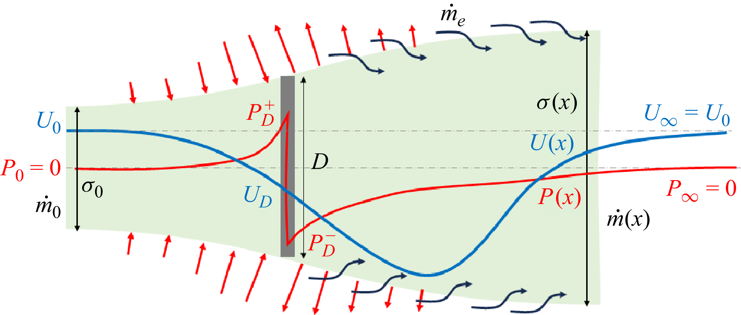
 σ(x)
σ(x) P=P(x)
 U=U(x)
 x=0
x=0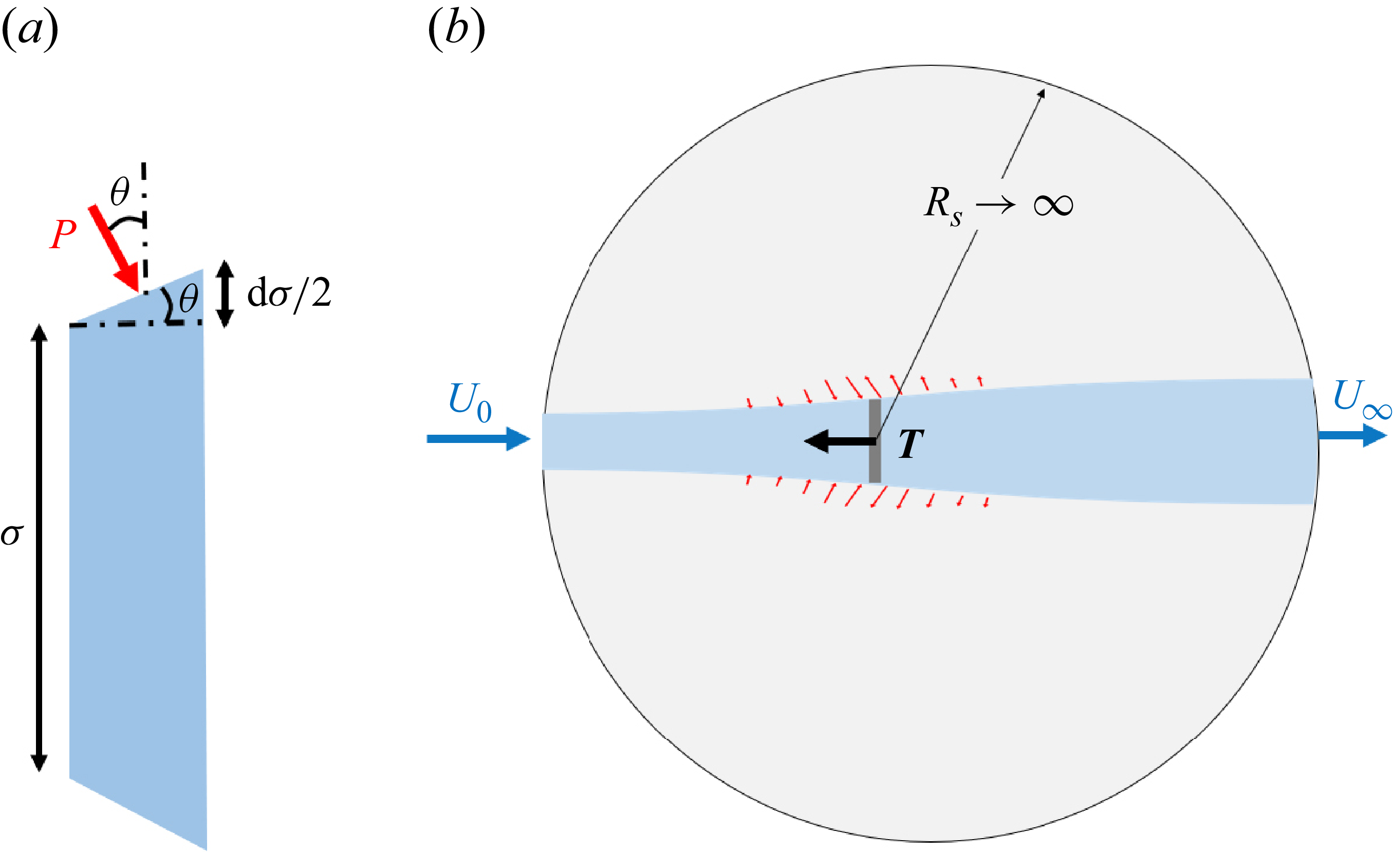
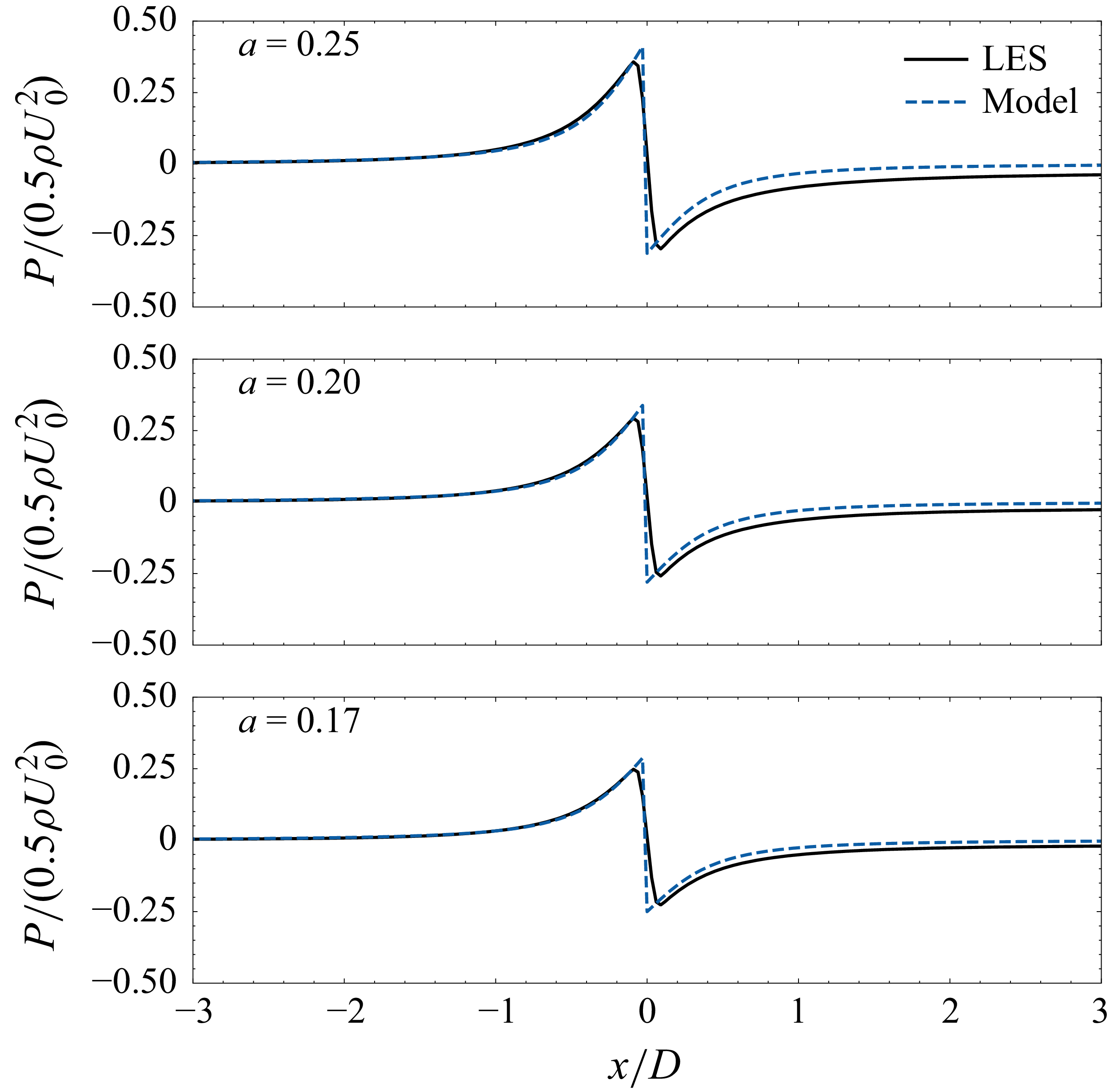
 E1
E1 E2=0.6
 I=0.05
 a=0.25
 a=0.45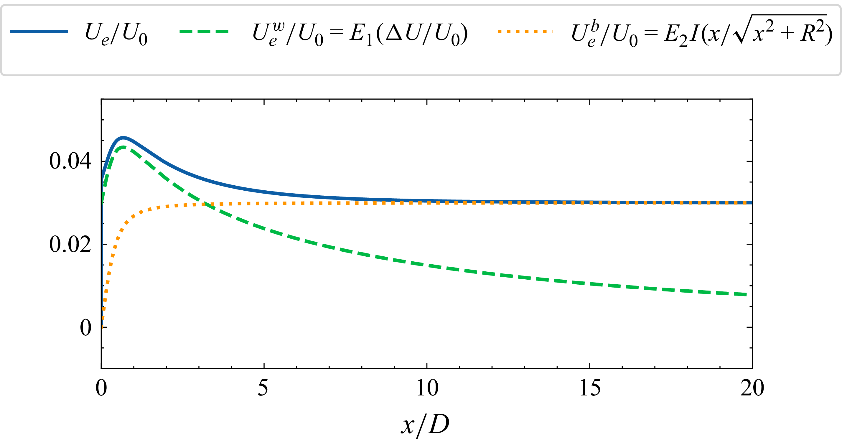
 Ue
Ue Uew
Uew Ueb
Ueb
 U
U σ
σ P
P a
a E1=0.1
 E2=0.6
 I=5%
I=5% U(x/D)/U0
 σ(x/D)/D
 P(x/D)/(1/2)ρU02
 a
a CT
CT E1
E1 E2
E2 I
I
 σ
σ x
x E1=0.1
 E2=0
E2=0 a
a σ
σ x
x E1=0.1
 E2=0.6
 a=0.3
a=0.3 I
I k=0.5dσ/dx
 x
x k∞
k∞
 U/U0
U/U0 P/(ρU02)
 CT=0.2
 CT=0.7
 I=10%
I=10% I=25%
I=25%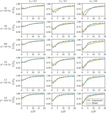
 U/U0
U/U0 CT∈{0.5,0.7,0.9}
 I
I 0.9%
0.9% 10.8%
10.8%
 σ/D
σ/D
 CT=0.8
 ΔU/U0
ΔU/U0 σ/D
σ/D I=6.9%
 9.4%
9.4% 13.4%
13.4% U
U σ
σ
 CT
CT CP
CP E1
E1 E2
E2 I=5%
I=5% CT
CT CT
CT CP
CP a
a E1
E1 E2
E2 I
I
 CT
CT CP
CP a
a CP
CP E1
E1 CP,max
 aopt
aopt E1
E1 E2
E2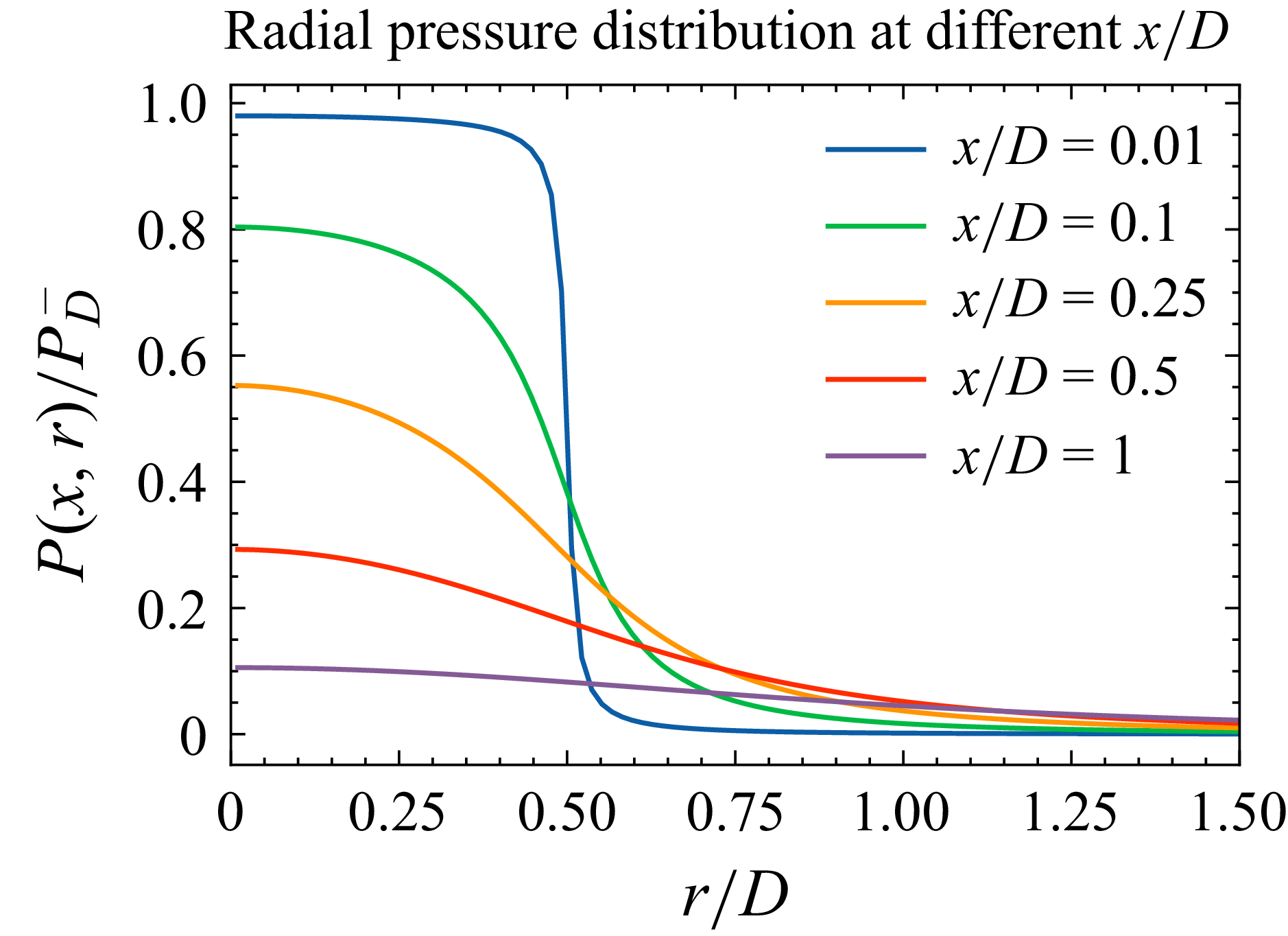
 P(x,r)
 PD−
PD−


 Open access

