


Introduction
Can biological species be recognized and delineated in the fossil record from morphology alone? This question is fundamental to most studies in evolutionary paleobiology, and only recently has the relationship between morphological and biological species been tested empirically (e.g., Bichain et al. Reference Bichain, Boisselier-Dubayle, Bouchet and Samadi2007; González-Wevar et al. Reference González-Wevar, Nakano, Cañete and Poulin2011; Reisser et al. Reference Reisser, Marshall and Gardner2012; Pieri et al. Reference Pieri, Inoue, Johnson, Smith, Harris, Robertson and Randklev2018; Smith et al. Reference Smith, Johnson, Pfeiffer and Gangloff2018; Vaux et al. Reference Vaux, Trewick, Crampton, Marshall, Beu, Hills and Morgan-Richards2018). The classic concept of a biological species (Mayr Reference Mayr1942) based on reproductive isolation is assumed to be manifested as well by a demonstrated lack of gene flow and in the clustering of organisms by size and shape. For this reason, some have claimed that morphological species, more often than not, proxy for biological species and can be identified and delimited with confidence (e.g., Gingerich Reference Gingerich1979; Bose Reference Bose2012)—and paleontologists can breathe a sigh of relief. Yet others claim that biological species can only be recognized reliably on the basis of molecular data (e.g., Hebert et al. Reference Hebert, Cywinska, Ball and deWaard2003; Robinson et al. Reference Robinson, Donald, Brandt and Lee2016)—and paleontologists have no truly robust basis upon which to recognize, and thus study, species. This possibility is obviously concerning to morphological paleontologists but is often assumed to be so uncommon that it can be disregarded with some confidence.
To test these opposing perspectives, we chose a clade in which individuals are abundant and diverse as fossils and are still living today. Brachiopods, terebratulide brachiopods in particular, meet these criteria and present a useful if somewhat frustrating combination of features that make them excellent study organisms. Like bivalved mollusks, they mineralize a bivalved shell that grows by accretion; unlike mollusks, they also mineralize a delicate and geometrically complex lophophore support structure called a brachidium, or “loop.” Because of their complexity, detailed morphological features of the loop have typically been used to distinguish extant species (Lee et al. Reference Lee, Carlson, Buening, Samson, Brunton, Cocks and Long2001) as well as higher taxa (MacKinnon and Lee Reference MacKinnon, Lee and Kaesler2006). However, because of their delicate structure, these distinguishing brachidial features are seldom preserved in fossils, particularly in Terebratellidina.
The questions we focus on in this study ask whether valve outline alone can clearly distinguish morphological clusters that proxy for biological species in Laqueus, a genus of terebratulide brachiopod. If so, how do valve outline morphometrics compare with long-looped brachidial morphometrics (López Carranza and Carlson Reference López Carranza and Carlson2019) in the delineation of morphological clusters? If we can answer yes to the first question, our confidence in using valve outline morphometrics to delineate biological species, both extant and extinct, will be greatly increased and, fortunately, can be tested further with DNA sequence data from extant individuals (López Carranza and Carlson Reference López Carranza and Carlson2018; N.L.C. and S.J.C. unpublished data). Answering the second question can increase our confidence that terebratulide valve outlines alone can provide sufficient distinguishing species-specific characteristics in the absence of brachidia, which are rarely preserved in fossils.
Laqueus Species
Our previous research (López Carranza and Carlson Reference López Carranza and Carlson2019) demonstrated that we can reliably differentiate among species of the genera Laqueus, Terebratalia, and Dallinella through the use of 3D geometric morphometric analysis of internal morphology, focusing on the long-looped brachidia. However, the relationship between valve shape and brachidial shape has not been quantified previously, and it is not clear if the two structures grow simultaneously in an integrated fashion with one another or grow in a more modular fashion, relatively independently of one another. Testing for a significant geometric relationship between them will help to illuminate the nature of their growth and modularity. It can also suggest hypotheses regarding the functional relationship between a particular lophophore configuration (indicated by the brachidial geometry), which facilitates respiration, feeding, and gamete release, and the relative shape and size of the mantle cavity (indicated by valve geometry), within which the lophophore must function. Investigating these ontogenetic and functional relationships is beyond the scope of this current study but presents intriguing directions for future research.
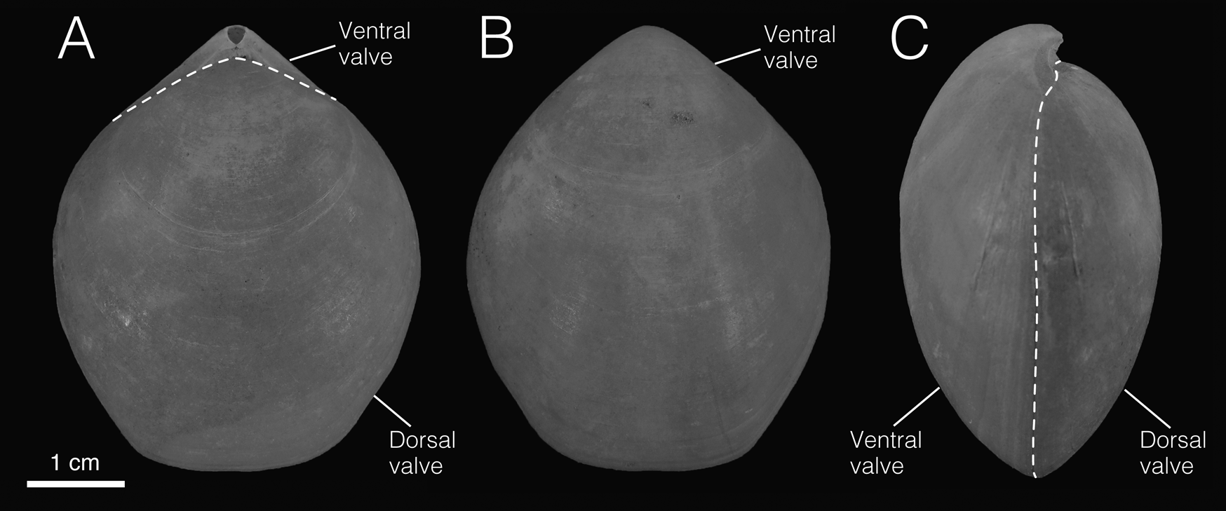
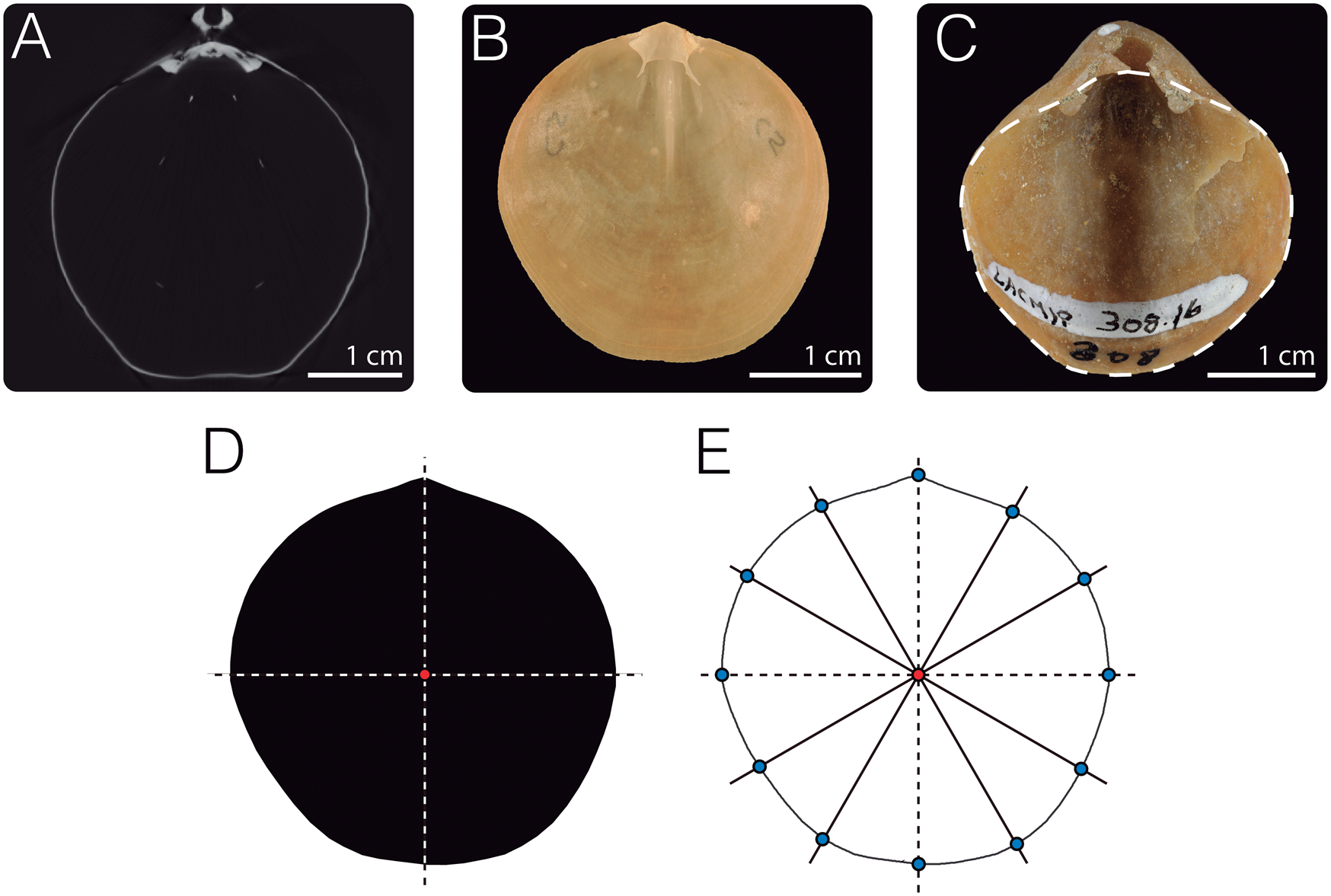
Brachiopod shells are commonly variable in outline shape between species and, in some cases, within species (Williams et al. Reference Williams, James, Emig, Mackay, Rhodes and Kaesler1997; see also Aldridge Reference Aldridge1981; Aldridge Reference Aldridge1999; Alexander Reference Alexander2001; Tort Reference Tort2003; Ruggiero et al. Reference Ruggiero, Raia and Buono2008; Bose Reference Bose2012; Robinson et al. Reference Robinson, Donald, Brandt and Lee2016). Compared with internal features, external shell shape is often assessed from a smaller number of characters and has been shown to be homeomorphic among some distantly related taxa (Buckman Reference Buckman1901; Cloud Reference Cloud1941; Stehli Reference Stehli and Moore1965; Cooper Reference Cooper1972, Reference Cooper1983; MacKinnon and Lee Reference MacKinnon, Lee and Kaesler2006). Shells of terebratulide brachiopods are commonly oval and elongated but range from subcircular (particularly in juveniles) to transverse (i.e., width > length; Lee and MacKinnon Reference Lee, MacKinnon and Kaesler2006). While some terebratulide species display a large range of variation in shell shape (e.g., species of the genus Terebratalia; Du Bois Reference Du Bois1916; Paine Reference Paine1969; Schumann Reference Schumann1991; Krause Reference Krause2004), others exhibit a more restricted spectrum of variability. This is the case of Laqueus Dall, Reference Dall1870, for which species possess shells that are variably ovate (MacKinnon and Lee Reference MacKinnon, Lee and Kaesler2006) but always maintain equal or larger length-to-width ratios throughout ontogeny. Laqueus is characterized by medium to large ovate shells with smooth exteriors (i.e., with no ornamentation) and a rectimarginate (i.e., planar) commissure (Dall Reference Dall1870; MacKinnon and Lee Reference MacKinnon, Lee and Kaesler2006) (Fig. 1). This genus has a temperate region, circum-Pacific distribution today, and is present in Cenozoic deposits of North America (Miocene?–Pleistocene; Hertlein and Grant Reference Hertlein and Grant1944) and Japan (Miocene; Hatai Reference Hatai1940), making it a good exemplar genus to compare living and fossil specimens, particularly given the complex history of identification of the two named species along the West Coast.
External morphology of Laqueus (Laqueus erythraeus CAS IZ 202358A). A, Dorsal view; B, ventral view; C, lateral view.
Thirteen extant Laqueus species are currently regarded as valid (Emig et al. Reference Emig, Bitner and Alvarez2019), with 10 species reportedly found around the coasts of Japan and the remaining three having a North American distribution (Hatai Reference Hatai1940 [who was known to have been a species “splitter”]; Logan Reference Logan, Kaesler and Selden2007; Zezina Reference Zezina2010). Here, we analyze five extant species of Laqueus (three with a Japanese distribution and two with a North American distribution), but we focus our study on Laqueus erythraeus and Laqueus vancouveriensis, because individuals of these species are distributed latitudinally along the eastern Pacific and are easily accessible in U.S. collections and we were able to obtain large samples of each.
Laqueus erythraeus Dall, Reference Dall1920 has been previously referred to as L. californicus or L. californianus due to a complicated history regarding naming and description (see MacKinnon and Long Reference MacKinnon and Long2000). Because of this, the complete morphological description of L. erythraeus (= L. californicus) can be found in Dall (Reference Dall1870). This species was originally described as having thin, oval-shaped biconvex shells with a planar commissure and a slightly truncated anterior edge. The beak is short, curved, and truncated obliquely, with a small pedicle foramen and conjunct deltidial plates. The cardinal plate (dorsal interior) is pentagonal with a very small cardinal process and concave inner hinge plates. The adult loop in all Laqueus species is bilateral (i.e., with horizontal and vertical connecting bands). Laqueus erythraeus is present off the coast of California, USA, today.
Laqueus vancouveriensis Davidson, Reference Davidson1887, described from specimens found off the coast of British Columbia, Canada, was originally considered to be a northern variety of L. californicus. Davidson described L. californicus var. vancouveriensis as small in size and circular to ovate in shape, with a truncated and slightly depressed anterior margin and a larger pedicle foramen than L. erythraeus. In a personal communication to Davidson in 1884, Dall described this northern variety as “thicker and ruddier” than L. erythraeus (Davidson Reference Davidson1887). Hertlein and Grant (Reference Hertlein and Grant1944) elevated L. vancouveriensis to full species rank based on its comparatively smaller shell size and larger foramen compared with L. erythraeus. This designation has been further reaffirmed qualitatively more recently (MacKinnon and Long Reference MacKinnon and Long2000). Laqueus vancouveriensis is distributed today from Alaska to Oregon, USA.
Species of the genus Laqueus were initially described based entirely on qualitative characterizations. Quantitative assessments of the differences and similarities between these species have been limited, however. López Carranza and Carlson (Reference López Carranza and Carlson2019) tested the validity of species groups within Laqueus, demonstrating that Laqueus species could be reliably distinguished based on 3D geometric morphometrics of brachidial and cardinalia morphology. Yet, because internal structures such as the brachidia are not commonly preserved in fossils (MacKinnon et al. Reference MacKinnon, Long, Owen, Harper, Long and Nielsen2008), analyses of delicate internal morphology can be less useful for paleontological inference, particularly if only partial individuals are preserved. Additionally, quantitative results can be difficult to compare with original species descriptions, which are heavily based on qualitative attributes. To date, there has been no investigation of species determination based on quantitative comparisons of external morphology.
Very few molecular phylogenetic analyses within the genus Laqueus exist. Saito and Endo (Reference Saito and Endo2001) examined the relationships among Laqueus species using COX1 sequences and found two highly supported, geographically distinct clusters: a Japanese group (L. rubellus, L. blanfordi, and L. quadratus) and a North American group (L. erythraeus [referred to as L. californicus] and L. vancouveriensis [referred to as L. c. vancouveriensis]). This analysis, however, did not assess differences between the two North American species and was not intended to examine species group validity or species delimitation. Noguchi and coauthors (Reference Noguchi, Endo, Tajima and Ueshima2000) sequenced the mitochondrial genome of L. rubellus, but species delimitation was not the purpose of their study. Species delimitation of Laqueus morphospecies using RAD (restriction site–associated DNA) markers has been analyzed by N.L.C. with results that validate morphologically based species designations (N.L.C. and S.J.C. unpublished data).
Valve Outline Characterization in Laqueus
Given how variable intraspecific valve outlines can be, they are generally not considered to be a reliable diagnostic character for species identification (Lee and MacKinnon Reference Lee, MacKinnon and Kaesler2006). Nonetheless, outlines have been used as qualitative features to describe and differentiate species of Laqueus, for example, Laqueus quadratus Yabe and Hatai, Reference Yabe and Hatai1934; Laqueus rubellus obessus Yabe and Hatai, Reference Yabe and Hatai1936; and Laqueus pacificus Hatai, Reference Hatai1936 (for a review of Japanese species of Laqueus, see Hatai Reference Hatai1940). The quantitative analysis of shell shape, with emphasis on valve outlines, has been applied to brachiopods to answer questions regarding overall morphological diversity (Smith and Bunje Reference Smith and Bunje1999), outline variation and taxonomic designations (Tort Reference Tort2003; Bose Reference Bose2012), substrate–shell shape relationships (Alexander Reference Alexander1975; Topper et al. Reference Topper, Strotz, Skovsted and Holmer2017), and fold/sulcus development (Lee et al. Reference Lee, Jung and Shi2018), as well as brachidial variability (Lee et al. Reference Lee, Carlson, Buening, Samson, Brunton, Cocks and Long2001).
Elliptical Fourier analysis (EFA) is one of the most frequently employed methodologies to study outlines, along with approaches such as geometric morphometric analyses of semilandmarks. EFA approximates outline shape through the sum of sine and cosine waves (Kuhl and Giardina Reference Kuhl and Giardina1982). Therefore, shape is described by harmonics, each representing a closed contour. The first harmonic models the general shape, while subsequent harmonics model smaller-scale shape variations. The number of harmonics used is determined by the number needed to represent most of the variation (Kuhl and Giardina Reference Kuhl and Giardina1982). Although the application of outline analysis has been limited in studies of brachiopods, outline methods have been more widely used in other groups, for example, bivalved mollusks (Ferson et al. Reference Ferson, Rohlf and Koehn1985; Crampton Reference Crampton1995; Rufino et al. Reference Rufino, Gaspar, Pereira and Vasconcelos2006; Scholz and Hartman Reference Scholz and Hartman2007; Wilk and Bieler Reference Wilk and Bieler2009; Márquez et al. Reference Márquez, Robledo, Peñaloza and Van der Molen2010; Neubauer et al. Reference Neubauer, Harzhauser and Mandic2013; Aguirre et al. Reference Aguirre, Richiano, Álvarez and Farinati2016), ostracods (Baltanás and Geiger Reference Baltanás, Geiger and Martens1998; Baltanás et al. Reference Baltanás, Brauneis, Danielopol and Linhart2003; Sánchez-González et al. Reference Sánchez-González, Baltanás and Danielopol2004; Liow Reference Liow2006; Danielopol et al. Reference Danielopol, Baltanás, Namiotko, Geiger, Pichler, Reina and Roidmayr2008; Tanaka Reference Tanaka2009), and insects (Rohlf and Archie Reference Rohlf and Archie1984; Monti et al. Reference Monti, Baylac and Lalanne-Cassou2001; Polihronakis Reference Polihronakis2006; Zhan and Wang Reference Zhan and Wang2012; Dujardin et al. Reference Dujardin, Kaba, Solano, Dupraz, McCoy and Jaramillo-O2014; Yang et al. Reference Yang, Ma, Wen, Zhan and Wang2015; Changbunjong et al. Reference Changbunjong, Sumruayphol, Weluwanarak, Ruangsittichai and Dujardin2016; Özkan Koca et al. Reference Özkan Koca, Moradi, Deliklitaş, Uçan and Kandemir2018).
The morphological features of Laqueus, particularly its rectimarginate (planar) commissure and the availability of both extant and fossil specimens, make this genus an excellent model for 2D valve outline analyses. This work aims to determine (1) whether a significant correlation exists between 2D valve outlines and 3D long-looped brachidia; (2) whether shell outlines alone can be used to reliably differentiate among extant terebratulide species; and (3) whether outline shape parameters in these specimens can be used as guidelines to test and distinguish fossil terebratulide species.
Materials and Methods
We analyzed two independent datasets to quantify outline variability, test the correlation between adult long-looped brachidial shape and shell outline, and build fossil species assignation models:
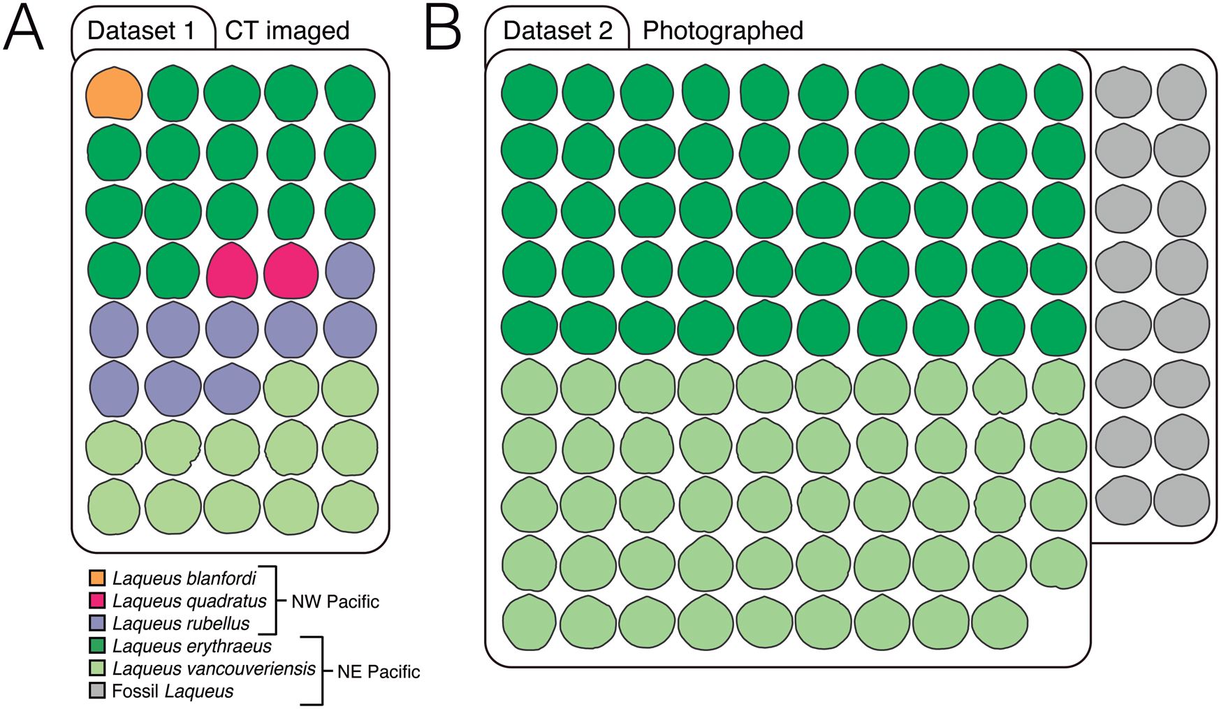
• Dataset 1: Outlines and long-loop landmarks and semilandmarks from extant Laqueus specimens imaged using computed tomography (CT) (Fig. 2A, Table 1).
• Dataset 2: Outlines of photographed extant and fossil Laqueus specimens (Fig. 2B, Table 2).
Datasets analyzed in this study. A, Dataset 1 consists of 40 computed tomography (CT)–imaged adult individuals classified in three extant species from the NW Pacific (Laqueus blanfordi [n = 1], Laqueus quadratus [n = 2], and Laqueus rubellus [n = 9]) and two from the NE Pacific (Laqueus erythraeus [n = 16] and Laqueus vancouveriensis [n = 12]) (Table 1). All specimens were CT imaged at the Center for Molecular and Genomic Imaging (CMGI) at the University of California, Davis. B, Dataset 2 consists of 99 photographed individuals of two extant species from the NE Pacific (L. erythraeus [n = 50] and L. vancouveriensis [n = 49]) and 16 fossil individuals from the Pliocene of Southern California (Table 2). Extant individuals were photographed by N.L.C. at the University of California, Davis. Fossil individuals were photographed by staff from the Natural History Museum of Los Angeles County Invertebrate Paleontology Collection. All outlines depicted in this figure are size-standardized.
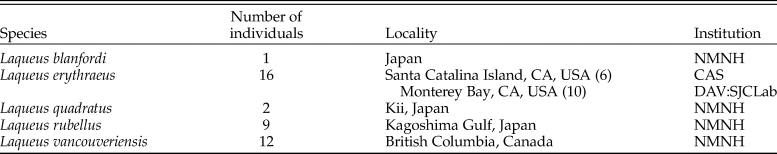
Dataset 1. List of computed tomography–imaged specimens analyzed including number of individuals, localities (NW and NE Pacific), and institutional collections from which specimens were obtained (NMNH, National Museum of Natural History, Smithsonian Institution; CAS, California Academy of Sciences; DAV:SJCLab, Carlson, personal collections, University of California, Davis). Small sample sizes reflect the logistical difficulties of collecting many species of extant brachiopods, not only Laqueus, and the collecting limits set by numerous institutions, given diminishing population sizes.
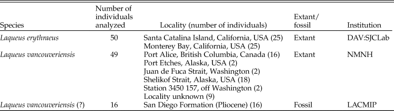
Dataset 2. List of photographed specimens analyzed including number of individuals, localities (NE Pacific), and institutional collections from which specimens were obtained (DAV:SJCLab, Carlson, personal collections, University of California, Davis; NMNH, National Museum of Natural History, Smithsonian Institution; LACMIP, Natural History Museum of Los Angeles County, Invertebrate Paleontology Collection).
Dataset 1: Analysis of Outline Variability and Correlation between Long-looped Brachidial Morphology and Shell Outline in Extant Laqueus
Specimens of dataset 1 (Fig. 2A, Table 1) were scanned at the Center for Molecular and Genomic Imaging (CMGI) at the University of California, Davis, using a MicroXCT-200 scanner from Carl Zeiss X-Ray Microscopy. To digitize the dorsal valve outlines, we sliced the image stacks for each specimen along the commissural plane using the software Amira v. 6.3.0 (Thermo Scientific), generating an image parallel to the planar commissure (Fig. 3A). These images were then manually traced in Adobe Illustrator CC 2018 to obtain black masks (the shell outline) against a white background. Each outline was scaled and rotated, aligning the umbo and centroid of the shell to the y-axis (Fig. 3D).
Outline digitization. A, For dataset 1, image stacks obtained from computed tomography (CT) were sliced parallel to the commissure to visualize the outlines of the dorsal valves of brachiopods. B,C, For dataset 2, individuals were photographed. In the case of extant specimens (B), dorsal valves were photographed; for fossil individuals, depending on the preservation of the specimens, dorsal, ventral, or complete shells were photographed (C). D, Images generated from A to C were manually traced using Adobe Illustrator to create black masks of the contour of the shells, which were then scaled and aligned. E, To digitize the outline coordinates, the black masks were input into the R package Momocs (Bonhomme et al. Reference Bonhomme, Picq, Gaucherel and Claude2014). Twelve landmarks were placed along the outlines to serve as the starting point for the Procrustes superimposition analyses. Specimens depicted: A, dorsal valve of Laqueus erythraeus CAS IZ 202358F; B, D, and E, dorsal valve of L. erythraeus DAV:SJCLab C5; C, ventral valve with inferred dorsal valve outline (dashed line) of Laqueus vancouveriensis LACMIP 308.30, LACMIP Type 14877.
To analyze variability in outline shape, we performed an outline analysis using the R packages Momocs (Bonhomme et al. Reference Bonhomme, Picq, Gaucherel and Claude2014) and Morpho (Schlager Reference Schlager, Zheng, Li and Székely2017). Outline coordinates were automatically extracted from the black-and-white JPEG files using Momocs (Bonhomme et al. Reference Bonhomme, Picq, Gaucherel and Claude2014) (Fig. 3E). To normalize outline coordinates before the EFA, we performed a generalized Procrustes analysis, which eliminates variation due to translation and rotation and standardizes scale according to centroid size (Rohlf and Slice Reference Rohlf and Slice1990; Frieß and Baylac Reference Frieß and Baylac2003; Zelditch et al. Reference Zelditch, Swiderski and Sheets2012). For the alignment of the outlines, 12 control landmarks were placed every 30° (Fig. 3E). The number of points was arbitrarily chosen and the landmark corresponding to the umbo (at 90°) was used as the homologous starting point for the alignments. After normalizing the outline data, an EFA was conducted using 99% of harmonic power (16 harmonics). The resulting elliptical Fourier coefficients were then used as input variables for a principal component analysis (PCA) to examine the overall pattern of variation and a canonical variate analysis (CVA) to determine if species could be discriminated based on outline shape. Along with the CVA, we performed a leave-one-out cross-validation (similar to a jackknife resampling) to obtain the overall classification accuracy by classifying each individual to one of the grouping variables (species) based on its morphological variables (Fourier coefficients).
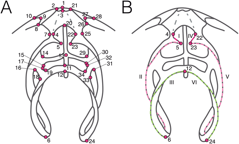
Landmarks and semilandmarks on the brachidia and cardinalia were digitized on 3D surface models using Stratovan Checkpoint (Stratovan Corporation) following an extension of our original landmark scheme that was limited to one side of the bilaterally symmetrical brachidium (Fig. 4; original scheme in López Carranza and Carlson [2019]; Supplementary Table S1). We added landmarks and curves on the right side of the loop and cardinalia to fully capture the overall loop shape, making them comparable to complete shell outlines.
Landmark and semilandmark scheme for long-looped brachidia. Schematic depiction of a bilateral long-looped brachidium showing the placement of the 34 landmarks (numbered in A and B) and six curves (roman numerals in B) used for the integration test between this structure and shell outlines.
Finally, to quantify morphological integration between long-looped brachidia and outlines, we performed a partial least-squares analysis (PLS). PLS evaluates the degree of shape covariation between two sets of variables (Bookstein Reference Bookstein, Marcus, Corti, Loy, Naylor and Slice1996, Reference Bookstein1998; Rohlf and Corti Reference Rohlf and Corti2000; Bookstein et al. Reference Bookstein, Gunz, Mitterœcker, Prossinger, Schæfer and Seidler2003; Adams and Felice Reference Adams and Felice2014; Adams and Collyer Reference Adams and Collyer2016), in this case, Procrustes-fitted (size removed) coordinates of brachidia and outlines. PLS was performed using the R package geomorph (Adams and Otárola-Castillo Reference Adams and Otárola-Castillo2013).
Dataset 2: Analysis of Outline Variability of Extant Specimens of L. erythraeus and L. vancouveriensis, and Machine Learning Classification of Fossil Specimens Using Random Forests Algorithm
To digitize the outlines of the extant specimens of dataset 2 (Fig. 2B, Table 2), we photographed the dorsal valve of disarticulated specimens (Fig. 3B). In the case of fossils, depending on the preservation of the individual, complete specimens and dorsal and ventral valves were photographed at the Natural History Museum of Los Angeles County (NHMLA). For dataset 1, the photographs were manually traced to obtain black masks (outlines) against a white background, scaled, and aligned (Fig. 3D). For fossils with articulated shells or only ventral valves, we inferred the outline shape of the dorsal valve by tracing the commissure of the opposing ventral valve (e.g., Fig. 3C) or the outline of the dorsal valve from a dorsal view (e.g., Fig. 1A). For the outline analysis of extant Laqueus erythraeus and L. vancouveriensis, we followed the same methodology as for dataset 1. We performed an EFA and subsequently implemented a PCA and a linear discriminant analysis (LDA) on the resulting elliptical Fourier coefficients, as well as a multivariate analysis of variance (MANOVA) to assess whether there is a significant difference between the outline shapes of L. erythraeus and L. vancouveriensis. Because size has been used as one of the species-defining characters in Laqueus (smaller individuals classified as L. vancouveriensis and larger as L. erythraeus), we decided to perform a second EFA without normalizing size (i.e., a partial Procrustes analysis only normalizing rotation and translation).
To test the classification of fossil specimens assigned tentatively to L. vancouveriensis, we trained two models based on shape variables/predictors (elliptical Fourier coefficients) using the random forests algorithm (Breiman Reference Breiman2001). Random forests is a supervised classification and regression algorithm; in other words, it uses a training dataset to predict the classification of new observations. This algorithm computes decision trees from bootstrap samples of a training dataset. For each tree, the nodes are split using a random subset of predictors (in this case, Fourier coefficients). New data can then be classified by combining the predictions of the generated trees (Breiman Reference Breiman2001). The rationale for implementing this methodology was to test fossil classification using a model informed by extant morphology. We built two models: one model based only on outline shape (i.e., normalizing size, rotation, and translation) and another based on both shape and size (i.e., normalizing size, rotation, and translation and reintroducing centroid size as a size variable). Machine learning analysis was performed using the R package randomForest (Liaw and Wiener Reference Liaw and Wiener2002).
All relevant data files for the analyses presented here are available from the Dryad Digital Repository: https://doi.org/10.5061/dryad.sqv9s4n23. The scripts are available on GitHub (https://doi.org/10.5281/zenodo.4275028).
Nonindependence of Elliptical Fourier Coefficients
It should be noted that EFA produces a large number of Fourier coefficients that are not independent from each other (Haines and Crampton Reference Haines and Crampton2000). In some cases, this can create issues for downstream analysis of EFA harmonic coefficient data. As described earlier, we primarily analyzed and characterized data using PCA and CVA. PCA is a method for identifying a small number of orthogonal (i.e., uncorrelated) components that explain a maximal amount of variance from a higher-dimensional set of intercorrelated/nonindependent components (Hammer and Harper Reference Hammer and Harper2006; Kim and Kim Reference Kim and Kim2012; Zelditch et al. Reference Zelditch, Swiderski and Sheets2012). Highly correlated initial component variables in a PCA are represented together by one or more principal component output variables that are orthogonal from other output principal components. CVA operates in a similar manner; however, unlike PCA, it maximizes separation based on group means. We consider PCA and CVA to be appropriate methods for characterizing interdependent data such as EFA harmonic coefficients. This is also why these ordination methods are so commonly used for 3D morphological landmark coordinates, which are also cocorrelated in complex ways.
To empirically validate these expectations, we reran some of our statistical tests. First, we recomputed all CVA/LDA procedures using PC scores as input variables. As principal components are orthogonal to each other, this should provide an alternate set of variables without cocorrelation. Additionally, as explained earlier, we built classification models using a random forests algorithm. It is possible that coefficient nonindependence could affect the classification models resulting from the random forests algorithm. But applying the same test method as that used for CVA/LDA—rerunning the statistical analysis using PC scores as inputs to ensure independent variables—has the potential to affect the results of a random forests analysis unpredictably. This is because, compared with the original data, principal components represent a transformation of the axes. While this is useful for many purposes, such as data visualization or certain kinds of machine learning analyses, it is uncertain whether the new axes generated by PCA are consistent with the discriminatory features of a supervised learning classification algorithm, such as random forests (Pechenizkiy et al. Reference Pechenizkiy, Tsymbal and Puuronen2004). Nonetheless, we also reran the random forests procedure using PC scores as input variables.
Results
Dataset 1: Outline Variability among Extant Species of Laqueus and Correlation with Long-looped Brachidial Shape
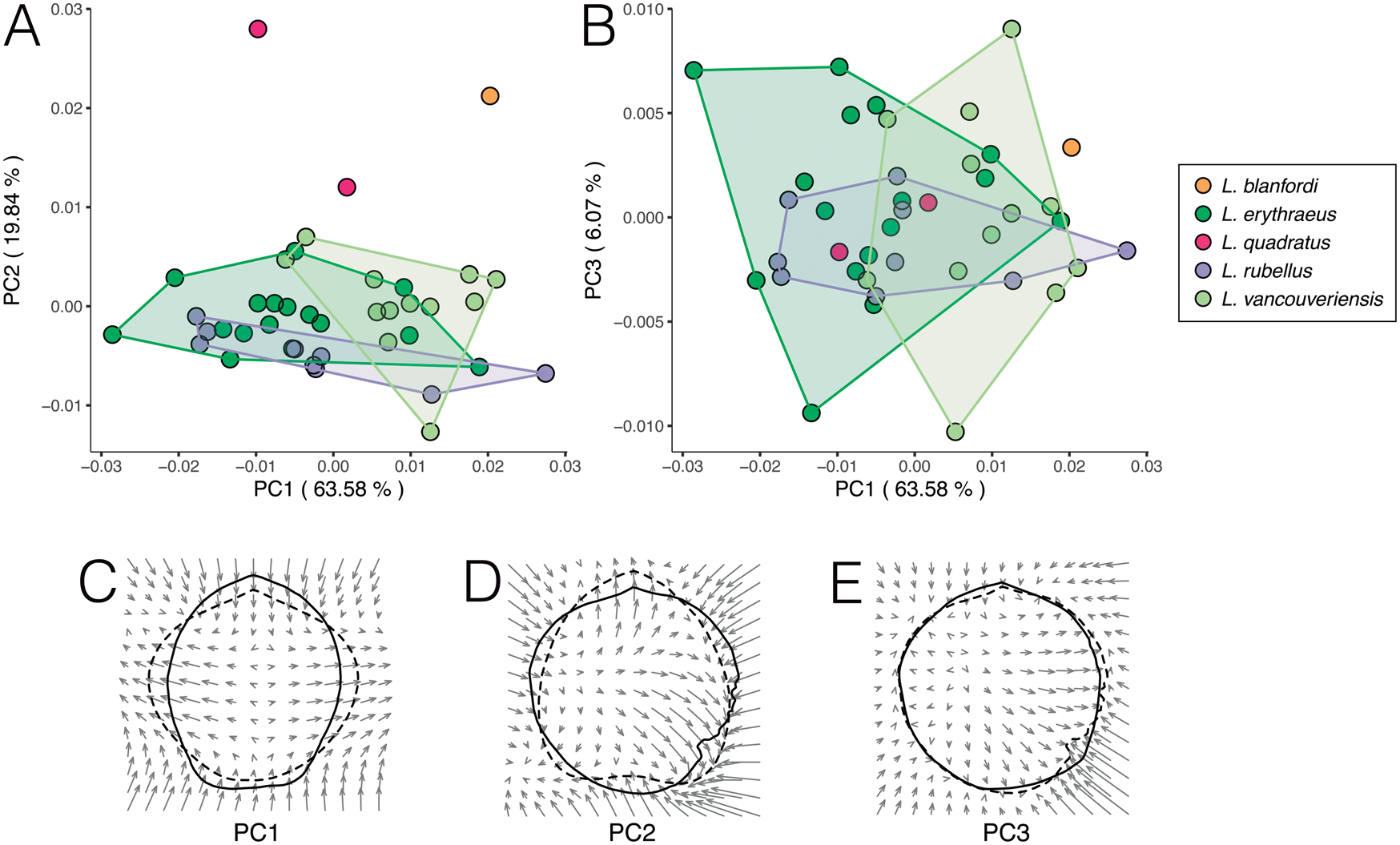
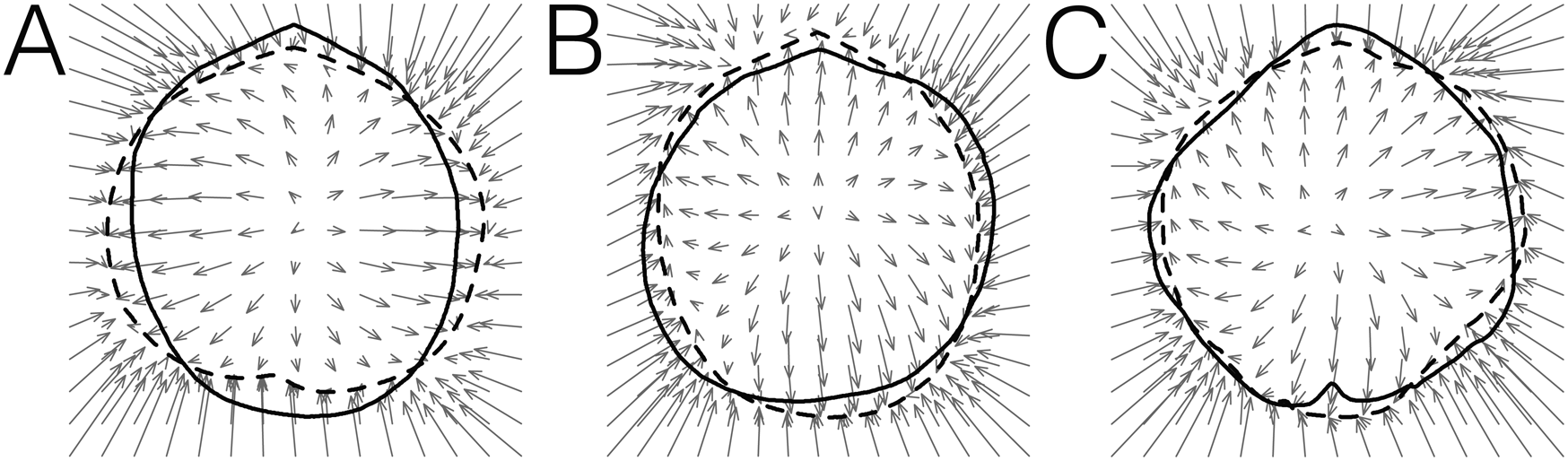
The overall pattern of outline variation in dataset 1 is shown in Figure 5A,B. Individuals of L. erythraeus, L. rubellus, and L. vancouveriensis display a significant overlap in morphospace, along PC 1 (63.58% variance), PC 2 (19.84% variance), and PC 3 (6.07% variance). Laqueus blanfordi and L. quadratus plot toward higher PC 2 values. In terms of outline shape, individuals with negative PC 1 values have elongated shells (length > width), while positive PC 1 values correspond to wider shells (width ~ length) (Fig. 5C). Plotted toward positive PC 2 scores, L. blanfordi and L. quadratus are characterized by having truncated or quadrate anterior margins (Dunker Reference Dunker1882; Yabe and Hatai Reference Yabe and Hatai1934), while negative PC 2 scores correspond to rounder shells (Fig. 5D). Outline shape change along PC 3 is mostly represented by small-scale differences in roundness; the specimen with maximum PC 3 score displays an irregular sinuate outline, commonly observed in L. vancouveriensis (Fig. 5E).
Principal component analysis (PCA) of dataset 1 on valve outlines described by elliptical Fourier coefficients and changes in outline shape corresponding to PCs. A, PC 1–PC 2; B, PC 1–PC 3. Thin-plate spline deformation vector fields showing shape change associated with C, PC 1 (PC 1min: Laqueus erythraeus DAV:SJCLab 0007; PC 1max: Laqueus rubellus USNM PAL 716075); D, PC 2 (PC 2min: Laqueus vancouveriensis USNM PAL 716058; PC 2max: Laqueus quadratus USNM PAL 716076); and E, PC 3 (PC 3min: L. vancouveriensis USNM PAL 716065; PC 3max: L. vancouveriensis USNM PAL 716058). Solid lines represent outlines corresponding to minimum PC values and dashed lines outlines corresponding to maximum PC values. Arrows represent the direction of shape change from minimum to maximum PC values.
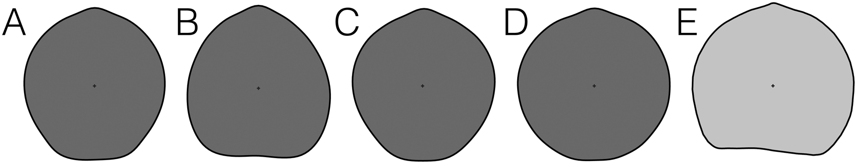
In terms of the mean shapes (average coordinate configuration for a group of specimens), each of the species analyzed exhibits a different overall shell shape (Fig. 6). Shells of Laqueus erythraeus tend to be elongated, with flat anterior commissures, and reach their widest point at the middle portion of the shell (Fig. 6A). Laqueus quadratus has a quadrate anterior margin, slightly curved medially; the widest part of the shell is located toward the anterior portion of the shell (Fig. 6B). Laqueus rubellus, on the other hand, has a similar shape to L. erythraeus, with a slightly flattened anterior margin; however, the widest part of the shell is located toward the posterior portion of the shell (Fig. 6C). Laqueus vancouveriensis shells are rounder, approximating a circular outline (Fig. 6D). For comparative purposes, we included the outline shape of the one analyzed specimen of L. blanfordi (Fig. 6E), which has a round outline, almost circular, but with a truncated anterior margin.
Mean shapes of A, Laqueus erythraeus; B, Laqueus quadratus; C, Laqueus rubellus; and D, Laqueus vancouveriensis. E, Outline of Laqueus blanfordi, represented by only one specimen.
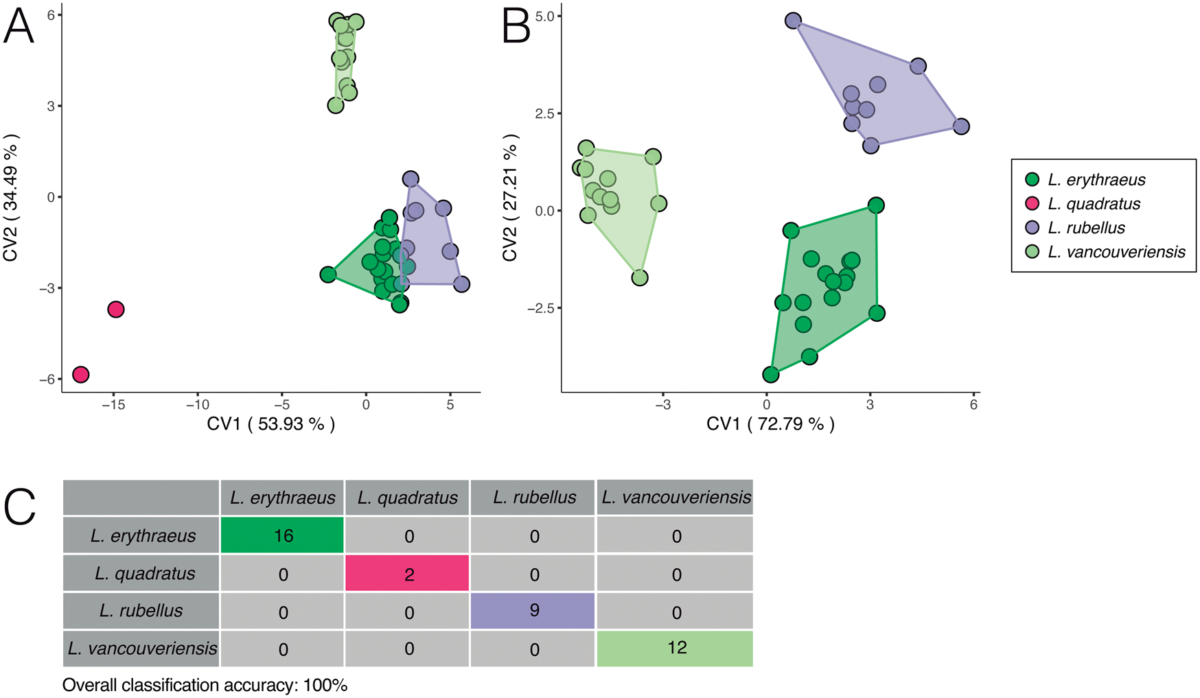
Despite the overlap in outline morphospace exhibited in the PCA, Laqueus species separate completely or almost completely in the CVA (Fig. 7). Compared with a PCA, CVA maximizes between-group variation, making it more effective at discriminating groups and separating them in morphospace. For the CVA, we excluded L. blanfordi, as we were able to obtain only one individual in our sample. When analyzing our dataset with L. quadratus (Fig. 7A), L. erythraeus and L. rubellus overlap slightly in shape space. Considering the mean outline shape of these two species (Fig. 6A and C, respectively), this result is not unexpected and is consistent with their similarities in shell outline, but not consistent with their geographic distributions on opposite sides of the Pacific Ocean. Laqueus vancouveriensis separated from these two species along CV 2. Laqueus quadratus, on the other hand, separates along both axes. When we excluded L. quadratus from our analysis (Fig. 7B), L. erythraeus, L. rubellus, and L. vancouveriensis separate completely, with L. vancouveriensis separating along CV 1 (72.8% variance) and L. erythraeus and L. rubellus separating along CV 2 (27.2% variance). Overall classification accuracy, obtained through a leave-one-out cross-validation, is 100%, with all specimens being correctly classified to their named species (Fig. 7C).
Canonical variate analyses (CVAs) on elliptical Fourier coefficients of dataset 1. A, CVA of Laqueus erythraeus, Laqueus quadratus, Laqueus rubellus, and Laqueus vancouveriensis. B, CVA excluding L. quadratus. C, Classification table based on a leave-one-out cross-validation (see text).
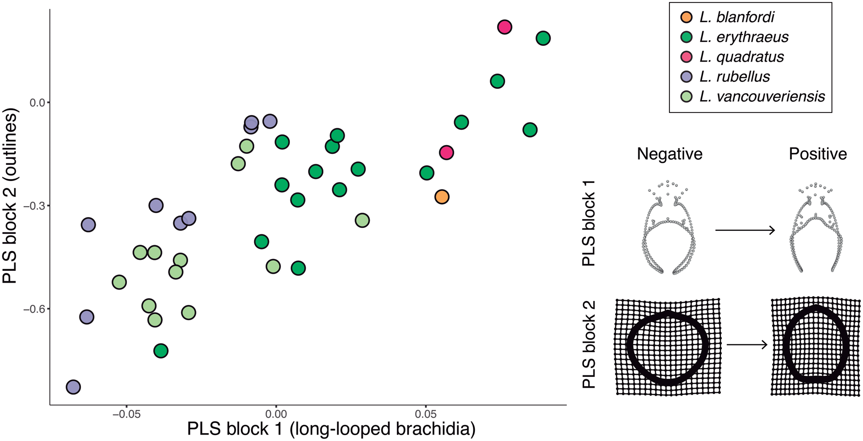
The PLS (Fig. 8), used to test morphological integration between shell outlines and long-looped brachidia, not including size, revealed a positive and statistically significant correlation between the two partitions (r-PLS = 0.773, p = 0.001). Cardinal and brachidial shape mirrors outline shape; for example, individuals with rounder anterior margins have terminal anterior loop extensions that draw more closely together relative to individuals with truncated anterior margins (e.g., the visualized positive and negative extrema in Fig. 8).
Plot of partial least-squares analysis PLS 1 scores for long-looped brachidial shape versus scores for outline shape. To the right, the maximal and minimal extrema of 3D landmark and semilandmark configurations for long loops (x-axis) and thin-plate spline of outlines (y-axis) are depicted. These extrema do not depict actual specimens, but rather show the most extreme shapes inferred from this model for each axis. The horizontal PLS 1 axis describes 3D landmark and semilandmark configurations, which vary from negative to positive extrema as shown above. The vertical PLS1 axis describes outlines, which vary from negative to positive extrema as shown above. As can be seen here, outline shape variation is associated with loop shape variation and vice versa.
Dataset 2: Outline Variation in Extant L. erythraeus and L. vancouveriensis
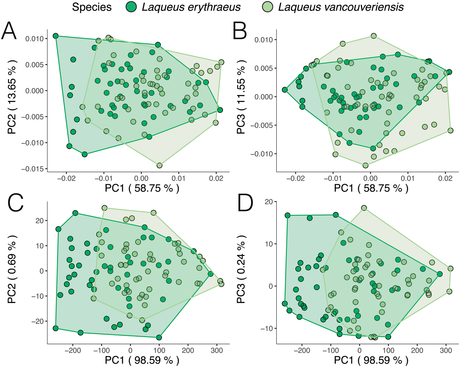
When analyzing outline variability in the extant specimens of dataset 2 (L. erythraeus n = 50, L. vancouveriensis n = 49), a PCA (Fig. 9) shows that these species overlap significantly in shape space. When looking only at variation in outline shape (Fig. 9A,B), both species display a similar distribution in morphospace, suggesting similar ranges of outline variability between L. erythraeus and L. vancouveriensis. The changes in shape along PC axes are shown in Figure 10. From negative to positive PC 1 scores (Fig. 10A), shells widen laterally and shorten in length. For PC 2 (Fig. 10B), minimum scores correspond to individuals with more circular outlines, while PC 2 maximum values are longer and narrower. Shape change along PC 3 (Fig. 10C) is mostly related to more subtle variations, such as deviations from the standard circular/elliptical shape, a common occurrence in L. vancouveriensis shells. The PCA results for the partially normalized outline analysis (Fig. 9C,D) show even more overlap between species, with most of the variation being due to differences in size. In terms of the mean shapes for both species, outlines are very similar; however, L. erythraeus, as previously shown in the results from dataset 1, has a more elongated shape, while L. vancouveriensis shells are rounder.
Principal component analysis (PCA) of extant individuals of Laqueus erythraeus and Laqueus vancouveriensis, color-coded by species. A, PC 1–PC 2, and B, PC 1–PC 3 of shell shape. C, PC 1–PC 2, and D, PC 1–PC 3 of shell shape and size.
Thin-plate spline deformation vector fields showing changes in outline shape associated with PC axes shown in Fig. 9A,B (size, rotation, and translation normalized). A, PC 1 (PC 1min: DAV:SJCLab C31; PC 1max: USNM PAL 770910); B, PC 2 (PC 2min: USNM PAL 770907; PC 2max: DAV:SJCLab C31); and C, PC 3 (PC 3min: USNM PAL 770881; PC 3max: USNM PAL 770892). Solid lines represent minimum PC values; dashed lines represent outlines associated with maximum PC values.
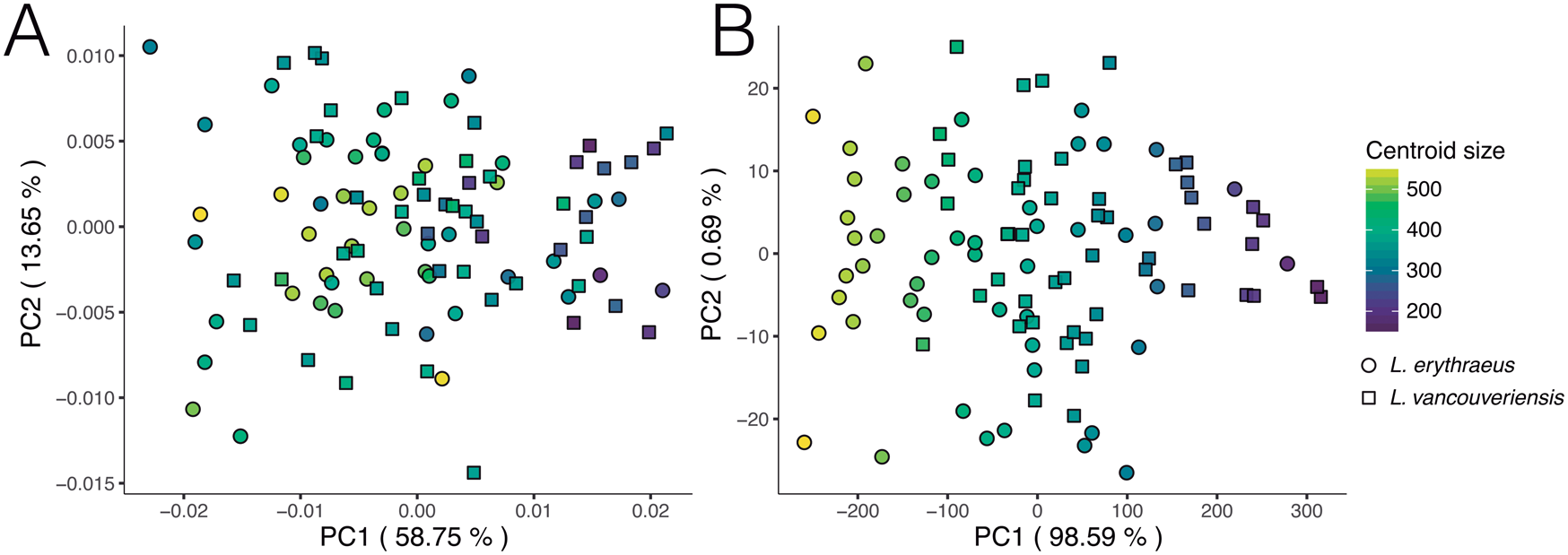
We reproduced and color-coded our PC plots (shown in Fig. 9) according to size (Fig. 11) and geographic locality (Fig. 12) to visualize size patterns and any latitudinal gradation that might exist in the data. To incorporate size into our results, we calculated centroid size. Centroid size is defined as the square root of the summed squared distances of each coordinate to the centroid of the configuration (Zelditch et al. Reference Zelditch, Swiderski and Sheets2012). Figure 11A (normalized size, rotation, and translation) shows that, in general, smaller individuals tend to have rounder shells and larger individuals tend to have more elongated shells. Although L. erythraeus adults are larger in size than L. vancouveriensis adults, these two species each exhibit a broad range of shapes and sizes. When size is not removed from our data, the variance associated with PC 1 (98.59%) is entirely driven by size (Fig. 11B).
Principal component analysis (PCA) of extant Laqueus erythraeus and Laqueus vancouveriensis, color-coded by centroid size. A, PC 1–PC 2 of shell shape; B, PC 1–PC 2 of shell shape and size.
Principal component analysis (PCA) of extant Laqueus erythraeus and Laqueus vancouveriensis, color-coded by geographic locality. A, PC 1–PC 2 of outline shape. B, PC 1–PC 2 of outline shape and size. C, Locality map. Because size was not normalized in B, larger individuals plot toward negative PC 1 values, and smaller individuals plot toward positive PC 1 values (see Fig. 11 for color-coded plots according to size).
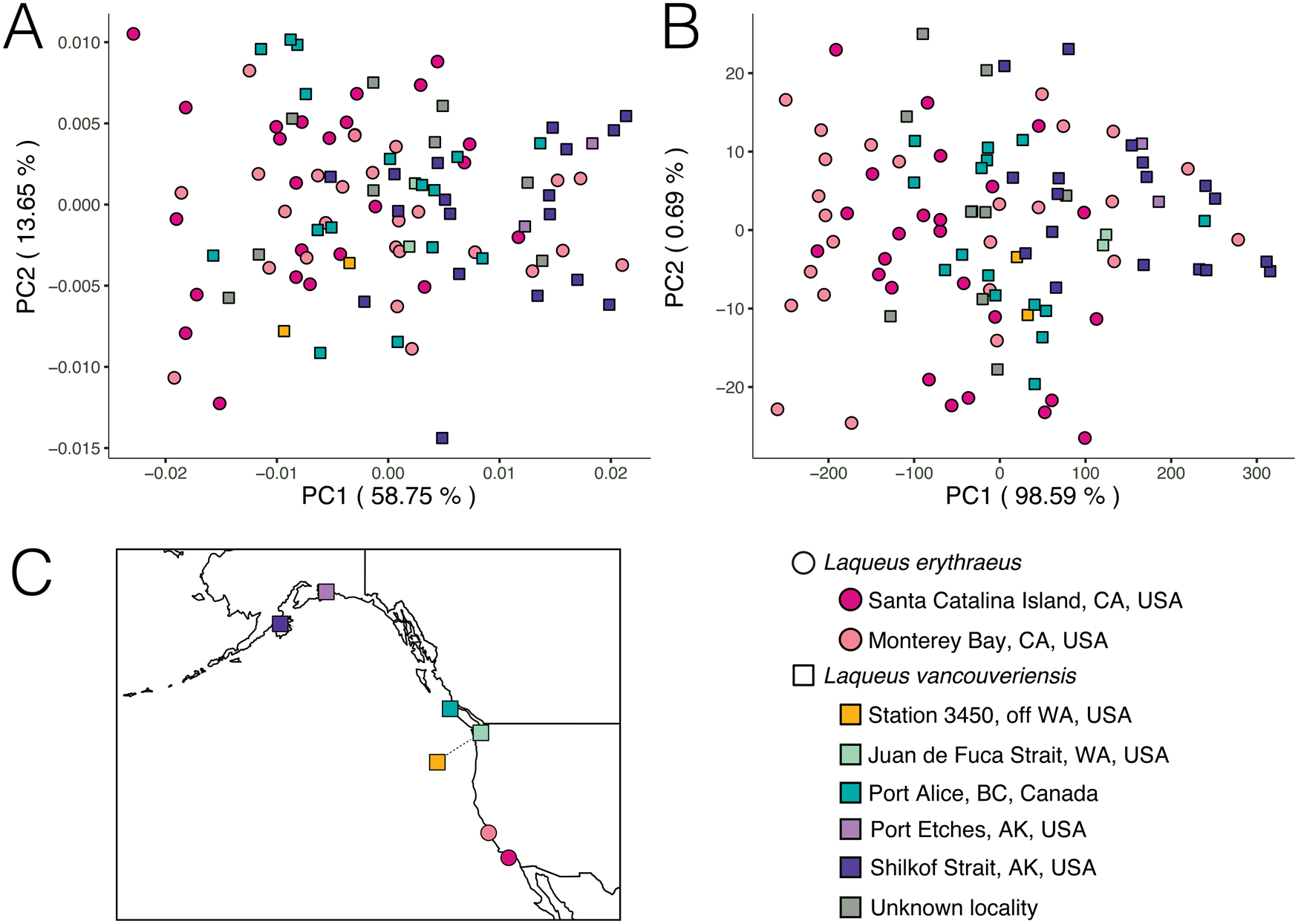
In terms of geographic localities, we were expecting to see a size–latitude gradient, with larger individuals in southern localities and smaller individuals in northern localities (i.e., converse Bergmann trend; Park Reference Park1949), regardless of species designation. We predicted this pattern due to the observation that smaller specimens of Laqueus occur at higher latitudes (e.g., Davidson Reference Davidson1887; Hertlein and Grant Reference Hertlein and Grant1944). In our first analysis (normalized size, rotation, and translation; Fig. 12A), individuals of L. erythraeus from Monterey Bay (light pink) and Santa Catalina Island (magenta) overlap in morphospace, with those from Santa Catalina Island displaying a somewhat smaller range of outline variability. For the second analysis (normalized rotation and translation; Fig. 12B), larger individuals correspond to L. erythraeus, particularly to those found in Monterey Bay. Individuals from Santa Catalina Island also plot toward lower PC 1 values but tend to be smaller than those found in northern California. This result suggests that our expected size–latitude gradient does not apply to Laqueus erythraeus (northern populations are larger in body size than southern populations), not confirming our expectations. In both Figure 12A and B, although not readily apparent, L. vancouveriensis individuals from Washington and British Columbia (yellow and blue/green points) tend to plot in intermediate PC 1 values, while Alaskan specimens (purple points) correspond to higher PC 1 values, corroborating the expected size–latitude gradation. Even though there is not a clear shape gradient between L. erythraeus and L. vancouveriensis, there is a shape gradient among individuals of L. vancouveriensis.
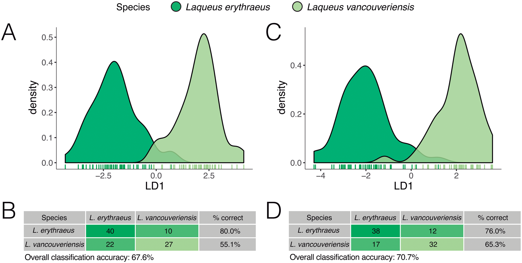
To examine separation between species, we conducted two LDAs—which maximize the separation between groups—on elliptical Fourier coefficients and a leave-one-out cross-validation test. In the first, we normalized size, rotation, and translation (full Procrustes); in the second, we only normalized rotation and translation (partial Procrustes). When only shape is considered, the result from the LDA shows that there is some overlap between the two species (Fig. 13A,B), with some specimens being classified erroneously. Specimens of L. erythraeus are classified correctly 80.0% of the time. In contrast, individuals of L. vancouveriensis are often misclassified as L. erythraeus 44.9% of the time (Fig. 13B). Overall classification correctness was 67.7% (i.e., 67 out of 99 individuals were classified correctly). Our LDA shows less overlap when considering both shape and size than when only accounting for shape (Fig. 13C). Furthermore, the overall classification accuracy increased by 3.1% (70.7%, 70/99 individuals classified correctly) (Fig. 13D). When considering size in our analysis, we see an increase in the classification accuracy of L. vancouveriensis from 55.1% to 65.3%.
Density plots of the first linear discriminant (LD 1). A, Density plot, and B, classification table based on a leave-one-out cross-validation for fully normalized outline data (only shape considered). C, Density plot, and D, classification table based on a leave-one-out cross-validation for partially normalized outline data (shape and size considered).
To test whether these species are statistically different in outline shape, we performed a MANOVA on elliptical Fourier coefficients, and our results show that these two species are significantly different (shape only: p < 0.01; shape + size: p < 0.01). To determine the effect size associated with this significant difference, we calculated eta-squared (shape only: η2 = 0.80; shape and size: η2 = 0.81) (Cohen Reference Cohen1988), which indicates a strong effect size signal in differences of shape between outlines of specimens belonging to these two species. This suggests a higher likelihood that the differences detected in these statistical samples do in fact reflect differences in actual species groups.
Fossil Classification Based on Random Forests Algorithm
To test and predict species assignation of the fossil Laqueus specimens (previously given the name L. vancouveriensis), we trained two models using the random forests algorithm, employing elliptical Fourier coefficients as shape predictors for L. erythraeus and L. vancouveriensis. Our first model was trained with the elliptical Fourier coefficients obtained from outlines where only shape was considered (size, rotation, and translation normalized); our second model used the elliptical Fourier coefficients from outlines where shape and size were both considered (size, rotation, and translation were normalized but size was reintroduced with a centroid size variable).
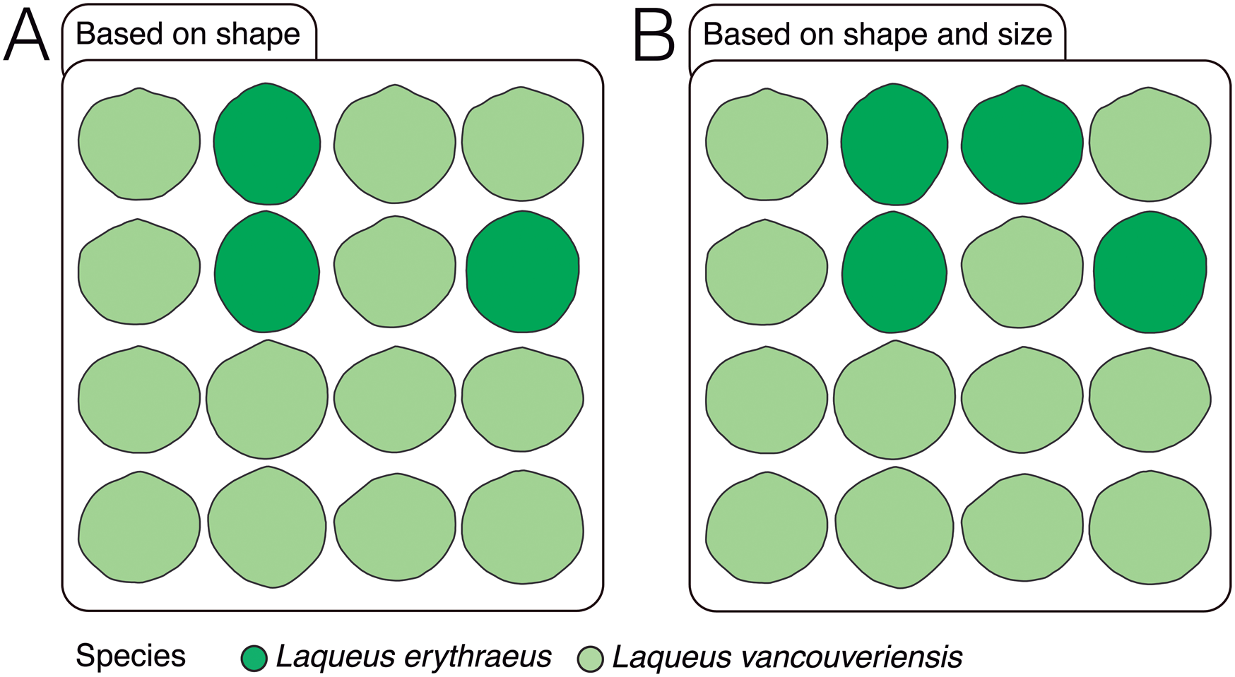
Given the similarity in outline shape between these species, the error rate for our first model was 20.2%, with L. erythraeus having a prediction error of 20.0% and L. vancouveriensis 20.4%. The random forests model classified 13/16 specimens as L. vancouveriensis and 3/16 as L. erythraeus. As expected, those classified as L. erythraeus have more elongated, less rounded shell outlines than L. vancouveriensis (Fig. 14A). These results are also consistent with the estimated error rate of 20.2%; the three individuals classified as L. erythraeus could be considered erroneously classified and represent 18.7% of the fossil dataset. Our second model has a lower error rate (18.18%), indicating that including size (or other informative variables) could improve classification. However, for our fossil test dataset, one larger individual was erroneously classified as L. erythraeus (Fig. 14B).
Predicted classification for fossil Laqueus specimens based on models built using random forests algorithm. A, Predicted classification when only shape is considered. B, Predicted classification when both shape and size are considered.
Nonindependence of Elliptical Fourier Coefficients
To test the effect of nonindependence of elliptical Fourier coefficients, we used PC scores as input variables for the CVA of dataset 1 and the LDA of dataset 2. The results obtained were identical to those from elliptical Fourier coefficients, confirming our initial expectations that it is appropriate in this case to use elliptical Fourier coefficients for the purpose of CVA/LDA. We also used PC scores as input variables for our random forests classification model. Compared with elliptical Fourier coefficients, the results were in fact notably different. This is consistent with the previously mentioned unpredictability of using PC scores with a random forests classification algorithm.
Discussion
Our study of Laqueus species focuses on achieving three objectives. First, to test the reliability of shell shape in discriminating extant Laqueus species, from two independent sets of valve outline data: from CT-imaged individuals identified to five species and from larger samples of photographed individuals of two of those species. Second, to test whether a significant correlation exists between 2D valve outlines and 3D brachidia in the same sample of individuals. Third, to determine whether outline shape parameters in extant species, whose identity as biological species can be tested with molecular data, could be used to establish the identity of extinct morphological species as biological species, which cannot be tested with molecular data.
Utility of Shell Shape in Discriminating Extant Laqueus Species from CT-imaged Specimens (Dataset 1)
In this first dataset, the PCA shows a significant overlap in outline morphospace (Fig. 5). The overlap in shape space is a result of high intraspecific variability and the fact that we are analyzing samples of simple, circular to oval outline shapes. Eastern Pacific species L. erythraeus and L. vancouveriensis appear to have larger ranges of variation than western Pacific L. rubellus. However, a larger sample size of L. rubellus would be needed to fully validate this difference in ranges of variability between eastern and western Pacific species. The CVA, which maximizes between-group variance relative to within-group variance, clearly separates the analyzed species in morphospace and shows less separation between L. erythraeus and L. rubellus (Fig. 7), indicating that these two species are more similar in shape than either is to L. vancouveriensis, even though L. erythraeus and L. vancouveriensis are both eastern Pacific species. Although they occur on opposites sides of the Pacific Ocean, L. erythraeus and L. rubellus were collected from similar latitudes and possibly similar temperature regimes (López Carranza and Carlson Reference López Carranza and Carlson2019). The similarity in outlines between L. erythraeus and L. rubellus is also visible in their mean outline shapes, shown in Figure 6. On the other hand, the mean outline shapes for L. vancouveriensis, L. quadratus, and L. blanfordi are more readily distinguishable.
Does a Significant Correlation Exist between Two-Dimensional Valve Outlines and Three-Dimensional Long-looped Brachidia in Laqueus Species?
From our previous studies (López Carranza and Carlson Reference López Carranza and Carlson2019), we concluded that we can quantitatively and reliably discriminate extant species based on long-loop brachidial morphology. However, delicate internal morphology, including brachidia, is rarely preserved in fossils.
The PLS to test morphological integration between loop shape and shell outline reveals a significant positive correlation (Fig. 8; r = 0.773, p = 0.001). Although outlines offer less resolution than internal morphology when discriminating among species, with sufficient sample sizes of individuals, outlines are a good proxy for taxonomically informative internal structures in Laqueus. In the case of fossil specimens, where internal structures are commonly missing, we can rely on outlines as valuable morphological variables, again with sufficient sample sizes. With this in mind and having more confidence now in the quantitative use of outlines, we analyzed a larger sample of extant individuals of L. erythraeus and L. vancouveriensis to create a dataset that would provide shape predictors to train a classification model for fossil specimens.
Utility of Shell Shape in Discriminating Extant Specimens Identified as L. erythraeus and L. vancouveriensis (Dataset 2)
To analyze our second dataset, we took two approaches, one only accounting for shape (i.e., we normalized size, rotation, and translation by implementing a full Procrustes superimposition) and another accounting for both shape and size (i.e., normalizing only rotation and translation using a partial Procrustes superimposition). Size has been considered one of the primary characteristics to distinguish L. erythraeus from L. vancouveriensis, with L. vancouveriensis being smaller overall than L. erythraeus (MacKinnon and Long Reference MacKinnon and Long2000). Our shape-only results (Fig. 9A,B) show that L. erythraeus and L. vancouveriensis have similar ranges of outline shape variation, with L. erythraeus having somewhat more elongated shells and L. vancouveriensis having somewhat rounder shells. The shape + size PCA results are almost entirely dominated by size, rather than shape (see Fig. 11B), consistent with the earlier qualitative studies noting differences between these two species.
Furthermore, there appears to be a latitudinal gradient in shape and size among individuals of L. vancouveriensis; the smaller, rounder forms are found in the most northern localities (Fig. 12). These differences suggest possible relationships to gradients in seasonal ocean temperatures, nutrient availability, extent of larval transport, and gene flow, populational variability, and speciation; relationships that are testable but beyond the scope of this study.
A shape + size latitudinal gradient is not found in L. erythraeus, but analyzing a larger number of localities across a greater latitudinal spread (Fig. 12) could potentially reveal a similar gradient, as seen in L. vancouveriensis. In terms of shape, the two populations of L. erythraeus overlap completely (Fig. 12A); in size, southern individuals (from Santa Catalina Island) are actually smaller, not larger, than northern individuals (from Monterey Bay) (Fig. 12B). Our LDA and cross-validation classification results show that when accounting for both outline shape and size, the overall classification accuracy is higher, driven by the improvement in the classification of L. vancouveriensis from 55.1% only considering shape to 65.3% considering both shape and size (Fig. 13).
Can Outline Shape Parameters in Extant Species Be Used to Establish the Identity of Extinct Morphological Species as Likely Biological Species?
Given the demonstrated value of outlines for species discrimination in extant Laqueus, we created two classification models to test species designation in fossil specimens. Our prediction models used elliptical Fourier coefficients as shape variables and were built using a machine learning algorithm of random forests relying on two a priori classes (L. erythraeus and L. vancouveriensis). Given this, a caveat is required to explain this choice. The classification model used is not necessarily well suited for the detection or identification of unknown classes or entirely new and previously unknown species. The difficulty of identifying “unknown” classes is one of the drawbacks of supervised classification algorithms. There are different ways to approach cases in which a new species or a species different from the ones in the training dataset could be present. For example, one can establish a probability threshold for the resulting classification (e.g., reject the result of ~50% probability for each category in a binary classification model and accept classifications with ≥60% probability). A more rigorous option is to start with a one-class classification method to determine whether a sample belongs to a general category, followed by a successively more detailed multiclass method. Finally, other machine learning methods could provide an alternative for recognizing new or unknown classes (e.g., open set recognition; Scheirer et al. Reference Scheirer, de Rezende Rocha, Sapkota and Boult2012).
We relied on extant morphological variables to predict fossil taxonomic designations; however, machine learning classification models can be based on any type of informative data (e.g., fossil morphology or biogeographical or paleoecological data). Machine learning models are currently underutilized in paleontology but have the potential to address a wide range of research questions (see Hsiang et al. Reference Hsiang, Brombacher, Rillo, Mleneck-Vautravers, Conn, Lordsmith, Jentzen, Henehan, Metcalfe, Fenton and Wade2019). Our study exemplifies one of the many paleobiological problems that can be tackled successfully using these methods.
Our test dataset consists of fossil individuals identified in the collections of the NHMLA as L. vancouveriensis from the Pliocene of Southern California (San Diego Formation). As discussed previously, extant individuals of Laqueus collected from California have all been referred more recently to L. erythraeus (previously L. californianus; MacKinnon and Long Reference MacKinnon and Long2000), not L. vancouveriensis, which has a geographic range today farther north than and non-overlapping with L. erythraeus (see Fig. 12C). According to Hertlein and Grant (Reference Hertlein and Grant1944), the stratigraphic ranges of both L. erythraeus and L. vancouveriensis in California extend back to the earliest Pliocene. Our study on valve outlines has the potential to test the identification of these Pliocene fossils: are they actually L. vancouveriensis, based on their size and shape, or are they L. erythraeus, based on the current biogeographic range of this species? Correct species identification and assigning names to museum specimens, both fossil and Recent, can play a significant role in investigations of morphological and biogeographic variability, as well as evolutionary patterns of change in populations and species over time.
Recall that using the elliptical Fourier coefficients that account for shape and size, our model had a lower error rate than when only shape was considered. In our shape-only model, individuals classified as L. erythraeus have elongated shells (length > width). In our shape + size model, one large specimen, as well as three elongated specimens, were classified as L. erythraeus. Most Pliocene specimens, which are smaller and have more rounded outlines, were classified in our study as L. vancouveriensis. When using a training dataset that includes extant specimens assigned to both of these two Laqueus species, Pliocene fossils from San Diego labeled in the NHMLA as L. vancouveriensis were classified predominantly and correctly as L. vancouveriensis, not L. erythraeus. Our results confirm that the biogeographic range of L. vancouveriensis extended much farther south in the Pliocene than it does currently, particularly given the extensive right-lateral movement of much of western California along the San Andreas and San Jacinto Faults since the Pliocene. Investigating further the paleobiogeographic and evolutionary implications of these patterns are beyond the scope of this study but will be profitably investigated further, particularly utilizing genetic analyses of multiple populations of these extant species (N.L.C. and S.J.C. unpublished data).
Our study demonstrates the utility of quantitative methods for the analysis of morphological characters that have been traditionally regarded as “less informative” (simple valve outlines) for the purposes of species determination. In the absence of more informative characters, in our case, long-looped brachidia, shell outlines are a valuable source of data for species discrimination, especially in the fossil record, and especially when morphology can be characterized quantitatively and analyzed statistically. This is welcome news for brachiopod paleontologists, as it supports the assumption that morphological species can be a reliable proxy for biological species and can be identified and delimited with confidence. Finally, using shape parameters from extant species as guidelines, we were able to build classification models using machine learning algorithms, an innovative methodology that can be used profitably to approach a wide range of paleontological questions.
Conclusions
1. Even though terebratulide shells are simple in their circular to oval outline shape, valve outlines can be used to reliably and quantitatively distinguish among adults of Laqueus species. Subtle variations in outline that can be perceived by the eye, which often encourage the naming of new species, can be verified quantitively. Elliptical Fourier coefficients are accurate descriptors of outline shape and allow us to test and, in this case, validate species assignations statistically.
2. Eastern Pacific Laqueus, whose species’ distinctions on the basis of morphology alone have been questioned, can be distinguished reliably based on outline shape alone and on shape and size together. Laqueus vancouveriensis exhibits a latitudinal gradient in both shape and size, with smaller, rounder individuals farther north. However, this gradient in shape and size was not observed in L. erythraeus, for reasons that have not yet been determined.
3. Our results corroborate a statistically significant morphological correlation between valve outlines and long-looped brachidia by using both 3D geometric morphometrics and 2D outlines in the same sample of individuals. This result demonstrates the utility of shell outlines in species delimitation as an acceptable alternative to internal features, namely the delicate brachidia, which are not commonly preserved in fossils. This correlation also suggests specific testable interactions between the growth and function of these two different elements of brachiopod morphology.
4. We can predict the species identity of fossil Laqueus species through machine learning algorithms by training models using extant species’ valve outlines as shape variables.
5. Our results confirm that the Pliocene biogeographic range of L. vancouveriensis, which extended from Alaska to Southern California, contracted significantly sometime post-Pliocene to extend no farther south than Oregon today.
6. If our study of Laqueus is any indication, studying extant terebratulide brachiopods and using machine learning techniques can help us better characterize and discriminate closely related biological species in the fossil record with greater confidence on the basis of morphology alone.
Acknowledgments
This work was partially supported by grants from the National Science Foundation (EAR 1147537 and DEB 1747704) to S.J.C.; and the Cordell Durrell Funds (UCD Department of Earth and Planetary Sciences) and Invertebrate Paleontology Collections Study Grant (NHMLA) to N.L.C. N.L.C. gratefully acknowledges support from Consejo Nacional de Ciencia y Tecnología (CONACYT), the University of California Institute for Mexico and the United States (UCMEXUS), and Secretaría de Educación Pública (SEP, México).
We would like to thank D. J. Rowland from the Center for Molecular and Genomic Imaging at the University of California Davis for CT imaging the specimens analyzed in this study. We acknowledge and thank A. Hendy, K. Estes-Smargiassi, and L. Walker for their help working at the NHMLA Invertebrate Paleontology Collection and M. Florence for facilitating access to the Invertebrate Paleontology Collection at the National Museum of Natural History. We also thank P. D. Roopnarine and S. A. Nadler for their helpful comments throughout this research study and on earlier versions of the article and J. H. Robinson and one anonymous reviewer for their insightful comments and suggestions.


 Open access