


1. Fundamentals of a collision model
1.1. Introduction
Froth flotation is a key process in the production of raw materials such as copper, gold and rare earths needed for a vast range of technological products. This physicochemical process is presently almost the only one used to separate these valuable minerals from other gangue materials (Yarar Reference Yarar2000; Nguyen & Schulze Reference Nguyen and Schulze2004; Fuerstenau et al. Reference Fuerstenau, Jameson and Yoon2007). Small and finely ground ore particles are fed into large flotation cells that are filled with water. In the case of mechanical flotation cells, air bubbles are injected, and the slurry is agitated by a mechanical rotor. The separation is achieved by the difference in hydrophobicity between the valuable minerals and the gangue material, with hydrophobic particles attaching to air bubbles and being transported to a surface froth, where they are recovered. Unwanted, hydrophilic material does not attach and settles to the bottom of the flotation cell. Chemical reagents serve to enhance the disparity in hydrophobicity among the particles, and to adjust the properties of the froth thereby optimising the operational conditions of the process (Nguyen & Schulze Reference Nguyen and Schulze2004).
The industrial application of the flotation process presents significant challenges. For example, the ore grades encountered in mining today range from single-digit percentages to even lower values (Crowson Reference Crowson2012; Calvo et al. Reference Calvo, Mudd, Valero and Valero2016). Furthermore, the demand for raw materials is increasing due to the shift towards greener and more environmentally friendly technologies (Vidal, Goffé & Arndt Reference Vidal, Goffé and Arndt2013). In particular, the availability of 17 minerals, including copper, silver and titanium, has been identified as critical to the success of this transition (Arrobas et al. Reference Arrobas, Hund, Mccormick, Ningthoujam and Drexhage2017; Hund et al. Reference Hund, La Porta, Fabregas, Laing and Drexhage2020; Tabelin et al. Reference Tabelin, Park, Phengsaart, Jeon, Villacorte-Tabelin, Alonzo, Yoo, Ito and Hiroyoshi2021). Considering the transition to a more environmentally friendly process, the impact of the flotation process on the environment itself constitutes a significant issue due to its energy consumption (Lelinski et al. Reference Lelinski, Govender, Dabrowski, Traczy and Mulligan2011; Tabosa, Runge & Holtham Reference Tabosa, Runge and Holtham2016) and waste handling (Phiri, Singh & Nikoloski Reference Phiri, Singh and Nikoloski2021; Grieco et al. Reference Grieco, Sinojmeri, Bussolesi, Cocomazzi and Cavallo2021) with their respective environmental impact. It is therefore of great importance to increase the efficiency and the sustainability of the flotation process.
To achieve this goal, improved flotation equipment and processes are required. A valuable instrument in the conceptualisation of flotation equipment and the examination of hydrodynamic process conditions are Euler–Euler simulation frameworks. In the past, these frameworks have been extensively employed in numerous flotation studies (Koh & Schwarz Reference Koh and Schwarz2003, Reference Koh and Schwarz2006, Reference Koh and Schwarz2007; Fayed & Ragab Reference Fayed and Ragab2015; Wang et al. Reference Wang, Ge, Mitra, Evans, Joshi and Chen2018; Shi et al. Reference Shi, Sommer, Rox, Eckert and Rzehak2022; Zürner et al. Reference Zürner, Kamble, Rzehak and Eckert2024; Draw & Rzehak Reference Draw and Rzehak2025). However, the accuracy of such simulations depends on the accuracy of the simulation models employed.
A variety of relevant subprocesses in flotation exist. Some of the most relevant ones are collision, particle–bubble attachment, particle detachment and entrainment. Their interplay is often contextualised using the first-order flotation rate constant
 $k_1$
defined as (Nguyen & Schulze Reference Nguyen and Schulze2004)
$k_1$
defined as (Nguyen & Schulze Reference Nguyen and Schulze2004)
 \begin{equation} k_{1}=Z_{pb}P_a(1-P_d), \end{equation}
where
 $Z_{pb}$
is the collision frequency between particles and bubbles,
$Z_{pb}$
is the collision frequency between particles and bubbles,
 $P_a$
is the probability of particle attachment and
$P_a$
is the probability of particle attachment and
 $P_d$
the probability of particle detachment. A major one of these subprocesses is the collision process, especially between particles and bubbles (Dai, Fornasiero & Ralston Reference Dai, Fornasiero and Ralston2000; Nguyen & Schulze Reference Nguyen and Schulze2004), as it is directly related to the flotation performance. Before a particle can attach to a bubble, it must first collide with the bubble, so that the number of attached particles captured by the bubbles is significantly influenced by the number of particle–bubble collisions (Duan, Fornasiero & Ralston Reference Duan, Fornasiero and Ralston2003; You et al. Reference You, Li, Liu, Wu, He and Lyu2017). The collision frequency is a function of the local relative velocity of the collision partners (Saffman & Turner Reference Saffman and Turner1956). As these local relative velocities are not resolved in large-scale simulations, a submodel is required, which is hence critical for the accuracy of the entire simulation.
$P_d$
the probability of particle detachment. A major one of these subprocesses is the collision process, especially between particles and bubbles (Dai, Fornasiero & Ralston Reference Dai, Fornasiero and Ralston2000; Nguyen & Schulze Reference Nguyen and Schulze2004), as it is directly related to the flotation performance. Before a particle can attach to a bubble, it must first collide with the bubble, so that the number of attached particles captured by the bubbles is significantly influenced by the number of particle–bubble collisions (Duan, Fornasiero & Ralston Reference Duan, Fornasiero and Ralston2003; You et al. Reference You, Li, Liu, Wu, He and Lyu2017). The collision frequency is a function of the local relative velocity of the collision partners (Saffman & Turner Reference Saffman and Turner1956). As these local relative velocities are not resolved in large-scale simulations, a submodel is required, which is hence critical for the accuracy of the entire simulation.
Modelling collisions in flotation poses particular challenges due to the specific parameter regime encountered. A variety of models to predict the collision frequency exist, with comprehensive reviews compiled by Dai et al. (Reference Dai, Fornasiero and Ralston2000), Hassanzadeh et al. (Reference Hassanzadeh, Firouzi, Albijanic and Celik2018) and Kostoglou et al. (Reference Kostoglou, Karapantsios and Oikonomidou2020b
). However, as will be shown later, many of the existing collision models are not suitable for application in typical conditions of flotation. This is primarily due to their design for different situations, the exclusion of swarm effects, the exclusion of effects resulting from size differences between particles and bubbles and the lack of coverage of size ranges present in flotation. Furthermore, some models have mathematical inconsistencies. All these models focus on the hydrodynamic modelling of the collision frequency
 $Z_{pb}$
. Effects such as the surface properties and deformation of particles and bubbles, surfactants used and particle entrainment are not covered by these models. To have a full description of the flotation process and to include these effects, the respective submodels for the other subprocesses, as highlighted in (1.1), are required (Wills & Finch Reference Wills and Finch2015; Wang et al. Reference Wang, Nguyen, Mitra, Joshi, Jameson and Evans2016; Safari & Deglon Reference Safari and Deglon2020).
$Z_{pb}$
. Effects such as the surface properties and deformation of particles and bubbles, surfactants used and particle entrainment are not covered by these models. To have a full description of the flotation process and to include these effects, the respective submodels for the other subprocesses, as highlighted in (1.1), are required (Wills & Finch Reference Wills and Finch2015; Wang et al. Reference Wang, Nguyen, Mitra, Joshi, Jameson and Evans2016; Safari & Deglon Reference Safari and Deglon2020).
In light of these observations, the present contribution puts forward a new model, the `integrated multisize collision model’ (IMSC), that predicts the collision frequency with a particular emphasis on the flotation process. To achieve a good representation of the collision rates, detailed data from direct numerical simulations (DNS) of the collision process in flotation is used. These data are employed to validate the basic modelling assumptions, to select appropriate submodels for each subprocess involved and to validate the entire collision model. The IMSC focuses on the hydrodynamically driven collision process in flotation.
The paper is laid out as follows. After detailing the requirements for collision models, the IMSC is derived in § 2. The overall model is then validated with own DNS data and data from the literature in §§ 3 and 4. Appendix A provides a concise overview of the model for the purpose of implementation.
1.2. Mechanisms creating relative motion
The occurrence of collisions is defined as the moment at which the surfaces of the two collision partners come into sufficiently close contact (Saffman & Turner Reference Saffman and Turner1956; Sundaram & Collins Reference Sundaram and Collins1997; Nguyen & Schulze Reference Nguyen and Schulze2004). For the sake of brevity and generality, mineral particles and bubbles are collectively referred to as collision partners or dispersed elements. Unlike some literature on multiphase flows, the term ’particle’ is used here to describe mineral particles in flotation processes, excluding bubbles. The index
 $p$
is used for particles, while the index
$p$
is used for particles, while the index
 $b$
is used for bubbles. A collision partner from either group is denoted by the index
$b$
is used for bubbles. A collision partner from either group is denoted by the index
 $\alpha$
. Two unspecified collision partners from either class are distinguished by
$\alpha$
. Two unspecified collision partners from either class are distinguished by
 $i$
and
$i$
and
 $j$
. Complying with the flotation literature, large particles are addressed as coarse, while small particles are termed fine.
$j$
. Complying with the flotation literature, large particles are addressed as coarse, while small particles are termed fine.
The collision frequency per unit volume,
 $Z_{\textit{ij}}$
, represents the number of collisions between collision partners of two classes
$Z_{\textit{ij}}$
, represents the number of collisions between collision partners of two classes
 $i$
and
$i$
and
 $j$
(Saffman & Turner Reference Saffman and Turner1956; Duan et al. Reference Duan, Fornasiero and Ralston2003). As the collision frequency depends on the number of suspended elements of the classes
$j$
(Saffman & Turner Reference Saffman and Turner1956; Duan et al. Reference Duan, Fornasiero and Ralston2003). As the collision frequency depends on the number of suspended elements of the classes
 $i$
and
$i$
and
 $j$
it is usually normalised by these numbers, defining the collision kernel
$j$
it is usually normalised by these numbers, defining the collision kernel
 $\varGamma _{\textit{ij}}$
(Saffman & Turner Reference Saffman and Turner1956), with
$\varGamma _{\textit{ij}}$
(Saffman & Turner Reference Saffman and Turner1956), with
 \begin{equation} \varGamma _{\textit{ij}}= \frac {Z_{\textit{ij}}}{N_iN_{\!j}}, \end{equation}
where the total number of dispersed elements of classes
 $i$
and
$i$
and
 $j$
present in the domain is denoted by
$j$
present in the domain is denoted by
 $N_i$
and
$N_i$
and
 $N_{\!j}$
, respectively. The collision kernel is equivalent to the flux of dispersed elements from class
$N_{\!j}$
, respectively. The collision kernel is equivalent to the flux of dispersed elements from class
 $j$
into a sphere of radius
$j$
into a sphere of radius
 $r_c$
around the centre of a dispersed element from class
$r_c$
around the centre of a dispersed element from class
 $i$
, which is termed collision radius. In mathematical terms, this reads (Saffman & Turner Reference Saffman and Turner1956)
$i$
, which is termed collision radius. In mathematical terms, this reads (Saffman & Turner Reference Saffman and Turner1956)
 \begin{equation} \varGamma _{\textit{ij}} = \int _{\theta =0}^{2\pi } \int _{\phi = 0}^{\pi } r_c^2 \sin (\phi ) \ w_{r}^{(+)} \mathrm{d} \phi \ \mathrm{d} \theta . \end{equation}
The collision radius
 $r_c$
is defined as the distance between the centres of the collision partners at the time of collision. In the case of spherical collision partners, it is the sum of the radii of the respective elements
$r_c$
is defined as the distance between the centres of the collision partners at the time of collision. In the case of spherical collision partners, it is the sum of the radii of the respective elements
 $r_c=r_i+r_{\!j}$
, the distance at which the surfaces of the collision partners touch. Furthermore,
$r_c=r_i+r_{\!j}$
, the distance at which the surfaces of the collision partners touch. Furthermore,
 $w_{r}$
is the radial component of the relative velocity between the collision partners. For the sake of convenience, positive values of
$w_{r}$
is the radial component of the relative velocity between the collision partners. For the sake of convenience, positive values of
 $w_r$
are denoted by
$w_r$
are denoted by
 $w_r^{(+)}=H(w_r)w_r$
, where
$w_r^{(+)}=H(w_r)w_r$
, where
 $H$
is the Heaviside function.
$H$
is the Heaviside function.
Due to continuity, incompressibility and under the assumption of homogeneous isotropic turbulence, Saffman & Turner (Reference Saffman and Turner1956) simplified (1.3) to
 \begin{equation} \varGamma _{\textit{ij}} = 2\pi r_c^2 w_{r,{\textit{rms}}}, \end{equation}
where
 $w_{r,{\textit{rms}}}$
is the root mean square (r.m.s.) of the radial relative velocity between the collision partners. In the literature, this approach is referred to as the spherical collision kernel. Equation (1.4) is an exact solution of (1.3) under the given conditions.
$w_{r,{\textit{rms}}}$
is the root mean square (r.m.s.) of the radial relative velocity between the collision partners. In the literature, this approach is referred to as the spherical collision kernel. Equation (1.4) is an exact solution of (1.3) under the given conditions.
Several mechanisms have been identified in the multiphase flow literature that cause relative motion between collision partners in turbulent flow (Saffman & Turner Reference Saffman and Turner1956; Abrahamson Reference Abrahamson1975; Kostoglou, Karapantsios & Matis Reference Kostoglou, Karapantsios and Matis2006; Meyer & Deglon Reference Meyer and Deglon2011; Kostoglou et al. Reference Kostoglou, Karapantsios and Oikonomidou2020b ). Here, the nomenclature of Kostoglou et al. (Reference Kostoglou, Karapantsios and Matis2006) is employed.
Mechanism I (shear) describes the motion of small, inertialess dispersed elements perfectly following the fluid streamlines. In this case, the relative velocity of the collision partners is caused by the fluid shear, i.e. the velocity gradient of the fluid. However, as this mechanism predominantly concerns small dispersed elements and, since the fluid velocity between two points is decorrelated at large scales (Sawford Reference Sawford1991), its efficacy is limited to the viscous subscale.
Mechanism II (accelerative drift) describes the drift of larger and heavier dispersed elements from the fluid streamlines due to their inertia. The dispersed elements primarily interact with the large-scale fluid eddies, and their velocity is only partially correlated or fully uncorrelated with the fluid velocity.
The motion of dispersed elements can be classified into these mechanisms based on their Stokes number, which describes the ratio of the response time of a dispersed element,
 $\tau _\alpha$
, to the characteristic scale of the fluid. For a given dispersed element of phase
$\tau _\alpha$
, to the characteristic scale of the fluid. For a given dispersed element of phase
 $\alpha$
, the Stokes number is given by
$\alpha$
, the Stokes number is given by
 \begin{align} && {\textit{St}}_\alpha =\frac {\tau _\alpha }{\tau _{\!f}}=\frac {d_\alpha ^2(\rho _\alpha /\rho _{\!f}+c_{\textit{AM}})}{18\nu \tau _\eta } && \alpha =i,j. \end{align}
In this expression, the Kolmogorov time scale
 $\tau _\eta =(\nu /\varepsilon )^{1/2}$
is used for the fluid response time,
$\tau _\eta =(\nu /\varepsilon )^{1/2}$
is used for the fluid response time,
 $\tau _{\!f}$
, with the turbulent dissipation rate
$\tau _{\!f}$
, with the turbulent dissipation rate
 \begin{equation} \varepsilon = 2\nu \langle {\unicode{x1D64E}} {\unicode{x1D64E}} \rangle , \end{equation}
where
 $\unicode{x1D64E}$
is the deformation rate tensor, and
$\unicode{x1D64E}$
is the deformation rate tensor, and
 $\nu$
is the molecular kinematic viscosity. The added mass is taken into account by the second term in the numerator of (1.5), with the default value of
$\nu$
is the molecular kinematic viscosity. The added mass is taken into account by the second term in the numerator of (1.5), with the default value of
 $c_{\textit{AM}}=0.5$
for single spherical dispersed elements (Kostoglou et al. Reference Kostoglou, Karapantsios and Matis2006; Meyer & Deglon Reference Meyer and Deglon2011). Mechanism I describes the limit of
$c_{\textit{AM}}=0.5$
for single spherical dispersed elements (Kostoglou et al. Reference Kostoglou, Karapantsios and Matis2006; Meyer & Deglon Reference Meyer and Deglon2011). Mechanism I describes the limit of
 ${\textit{St}}_\alpha =0$
, while Mechanism II assumes very large but finite Stokes numbers (Abrahamson Reference Abrahamson1975; Meyer & Deglon Reference Meyer and Deglon2011). Typical real-world Stokes numbers in flotation for particles are in the range of
${\textit{St}}_\alpha =0$
, while Mechanism II assumes very large but finite Stokes numbers (Abrahamson Reference Abrahamson1975; Meyer & Deglon Reference Meyer and Deglon2011). Typical real-world Stokes numbers in flotation for particles are in the range of
 ${\textit{St}}_p\approx 0.1$
to
${\textit{St}}_p\approx 0.1$
to
 ${\textit{St}}_p\approx 8$
(Yuu Reference Yuu1984; Chan, Ng & Krug Reference Chan, Ng and Krug2023). Consequently, the motion of these particles is determined by a combination of these mechanisms.
${\textit{St}}_p\approx 8$
(Yuu Reference Yuu1984; Chan, Ng & Krug Reference Chan, Ng and Krug2023). Consequently, the motion of these particles is determined by a combination of these mechanisms.
Gravity is a third mechanism causing relative motion between collision partners, introducing a deterministic component to the relative velocity between collision partners of different masses in cases of different sizes or densities.
1.3. Requirements imposed on collision models in flotation
The conditions of flotation are highly challenging for collision models. To be considered suitable for application in the context of flotation, a collision model must meet the following requirements.
-
(i) The model should include all relevant mechanisms causing relative motion between bubbles and particles. As highlighted above, these are turbulent shear (Mechanism I), inertial drift of the collision partners (Mechanism II) and deterministic motion due to gravity.
-
(ii) Especially in the case of particle–bubble collisions, there is a significant size difference between the collision partners. The larger of the two, usually the bubble, distorts the surrounding flow field. This, in turn, affects the motion of the smaller particles and alters the resulting collision frequency (Kostoglou et al. Reference Kostoglou, Karapantsios and Oikonomidou2020b ). The collision model should take these flow field distortions into account.
-
(iii) A general collision model should be able to cover the broad range of particle and bubble diameters encountered in flotation, extending from the submicron scale of particles to the millimetre range of bubbles, as well as encompassing the variability in the diameter of particles, which can range from single-digit micrometres to several hundred micrometres (Deglon, Egya-Mensah & Franzidis Reference Deglon, Egya-mensah and Franzidis2000; Ostadrahimi et al. Reference Ostadrahimi, Farrokhpay, Gharibi and Dehghani2020).
-
(iv) Flotation involves dense swarms of bubbles and particles. Therefore, the model should account for swarm effects and not just individual bubbles and particles.
-
(v) The model is required to be mathematically consistent. This entails, for instance, that the various components of the model should be formulated within a common frame of reference and the employed submodels should be valid for the specified parameter range.
Most of the available models in the literature, however, were developed for purposes other than flotation and do not meet all the requirements listed above. Detailed reviews of existing collision models were compiled by Nguyen et al. (Reference Nguyen, An-Vo, Tran-Cong and Evans2016), Hassanzadeh et al. (Reference Hassanzadeh, Firouzi, Albijanic and Celik2018) and Kostoglou et al. (Reference Kostoglou, Karapantsios and Oikonomidou2020b ) for example. A brief summary of the relevant models is given in Appendix C for convenience.
2. Integrated multisize collision model
2.1. Basic structure
From the discussion above, it is to be concluded that a significant proportion of the models previously discussed are unable to simultaneously satisfy all the listed requirements. Moreover, numerous models exhibit substantial discrepancies between their results and those obtained from the DNS, as previously highlighted in the literature (Nguyen et al. Reference Nguyen, An-Vo, Tran-Cong and Evans2016; Kostoglou et al. Reference Kostoglou, Karapantsios and Oikonomidou2020b ; Chan et al. Reference Chan, Ng and Krug2023; Tiedemann & Fröhlich Reference Tiedemann and Fröhlich2025). Consequently, a new model, designated as the IMSC, is proposed here. It integrates established concepts from the literature together with new components and is applicable to a wide range of parameters for collision partners of varying sizes. The general approach is outlined in figure 1.
Schematic overview of the framework of the IMSC indicating input and output quantities, as well as the different components of the model together with the main data determined in intermediate steps. Nomenclature introduced in the text.

Flotation, overall, is a multiscale process ranging from the large-scale fluid structures in the entire flotation cell to the surface chemistry effects responsible for the attachment and detachment of particles. For the collision process the most important turbulence scales are those of the size of the collision partners up to a small multiple. Collisions are caused due to relative motion of the collision partners. Large-scale structures cause no relative motion on neighbouring dispersed elements. These structures rather impose a common velocity, not leading to a relative velocity and thus no collisions. Significantly smaller turbulent structures barely affect the motion of the collision partners also not leading to sizeable relative motion. Hence, the IMSC and its input parameters only refer to the local conditions at a scale approximately the size of the collision partners considered.
In figure 1 the input parameters of the IMSC contain two groups. Some immediately result from the physical system, such as the size and density of the dispersed elements,
 $r_\alpha$
and
$r_\alpha$
and
 $\rho _\alpha$
, as well as the fluid density and viscosity,
$\rho _\alpha$
, as well as the fluid density and viscosity,
 $\rho _{\!f}$
and
$\rho _{\!f}$
and
 $\nu _{\!f}$
, and the surface tension,
$\nu _{\!f}$
, and the surface tension,
 $\sigma _{bf}$
. The others are available in the context of a Reynolds-averaged Euler–Euler framework, like the turbulent kinetic energy
$\sigma _{bf}$
. The others are available in the context of a Reynolds-averaged Euler–Euler framework, like the turbulent kinetic energy
 $k$
and the dissipation rate
$k$
and the dissipation rate
 $\varepsilon$
. The volume fractions
$\varepsilon$
. The volume fractions
 $\epsilon _\alpha$
are also computed with such an approach, together with the velocity of all components, resulting in the Reynolds numbers of the dispersed elements,
$\epsilon _\alpha$
are also computed with such an approach, together with the velocity of all components, resulting in the Reynolds numbers of the dispersed elements,
 ${\textit{Re}}_\alpha$
. The desired output of the model is the collision kernel, which in the first place is used for particle–bubble collisions, but can also be evaluated for particle–particle, as well as for bubble–bubble collisions, if desired. In a large Euler–Euler simulation, which does not resolve individual dispersed elements or fine-scale fluid turbulence, the conditions vary over large scales in space and time. The modelling discussed here is local and addresses local quantities. The physical system considered can, hence, be interpreted as the one inside a single computational cell of an Euler–Euler simulation.
${\textit{Re}}_\alpha$
. The desired output of the model is the collision kernel, which in the first place is used for particle–bubble collisions, but can also be evaluated for particle–particle, as well as for bubble–bubble collisions, if desired. In a large Euler–Euler simulation, which does not resolve individual dispersed elements or fine-scale fluid turbulence, the conditions vary over large scales in space and time. The modelling discussed here is local and addresses local quantities. The physical system considered can, hence, be interpreted as the one inside a single computational cell of an Euler–Euler simulation.
The IMSC is based on the spherical collision kernel given in (1.4). The spherical collision kernel consists of two main components, the collision radius,
 $r_c$
, and the radial component of the relative velocity between the collision partners,
$r_c$
, and the radial component of the relative velocity between the collision partners,
 $w_{r,{\textit{rms}}}$
. As the collision radius is directly specified by the given system, i.e. the radii of the collision partners, modelling of the collision kernel is effectively reduced to modelling the radial relative velocity between the collision partners,
$w_{r,{\textit{rms}}}$
. As the collision radius is directly specified by the given system, i.e. the radii of the collision partners, modelling of the collision kernel is effectively reduced to modelling the radial relative velocity between the collision partners,
 $w_{r,{\textit{rms}}}$
.
$w_{r,{\textit{rms}}}$
.
Following the decomposition approach of Yuu (Reference Yuu1984), the radial component of the relative velocity,
 $w_r$
is decomposed into the contributions from Mechanism I, Mechanism II and gravity. For both components, a stochastic approach based on a Gaussian distribution of the velocity of the collision partners is followed. The modelling thus focuses on the description of the variance
$w_r$
is decomposed into the contributions from Mechanism I, Mechanism II and gravity. For both components, a stochastic approach based on a Gaussian distribution of the velocity of the collision partners is followed. The modelling thus focuses on the description of the variance
 $\sigma ^2$
of the velocity distribution (Yuu Reference Yuu1984; Kruis & Kusters Reference Kruis and Kusters1997; Ngo-Cong, Nguyen & Tran-Cong Reference Ngo-Cong, Nguyen and Tran-Cong2018). It is well known that real-world bubbles and particles in turbulent flow do not fully obey a Gaussian velocity distribution (Wang et al. Reference Wang, Chen, Brasseur and Wyngaard1996; Angriman, Mininni & Cobelli Reference Angriman, Mininni and Cobelli2020). However, the literature suggests that a reasonable approximation for the first two moments of the velocity distribution of the dispersed elements is close to those of a Gaussian distribution (Wang et al. Reference Wang, Chen, Brasseur and Wyngaard1996). The suitability of this approximation is confirmed in § 3.3. Gravity causes a deterministic velocity component that is independent of the fluid motion. As Mechanism II describes the motion of the dispersed elements relative to the fluid, its velocity distribution is combined with that obtained by gravity. In case of a substantial size difference between the collision partners, the disturbances of the fluid flow of the larger collision partner are taken into account using a correction factor,
$\sigma ^2$
of the velocity distribution (Yuu Reference Yuu1984; Kruis & Kusters Reference Kruis and Kusters1997; Ngo-Cong, Nguyen & Tran-Cong Reference Ngo-Cong, Nguyen and Tran-Cong2018). It is well known that real-world bubbles and particles in turbulent flow do not fully obey a Gaussian velocity distribution (Wang et al. Reference Wang, Chen, Brasseur and Wyngaard1996; Angriman, Mininni & Cobelli Reference Angriman, Mininni and Cobelli2020). However, the literature suggests that a reasonable approximation for the first two moments of the velocity distribution of the dispersed elements is close to those of a Gaussian distribution (Wang et al. Reference Wang, Chen, Brasseur and Wyngaard1996). The suitability of this approximation is confirmed in § 3.3. Gravity causes a deterministic velocity component that is independent of the fluid motion. As Mechanism II describes the motion of the dispersed elements relative to the fluid, its velocity distribution is combined with that obtained by gravity. In case of a substantial size difference between the collision partners, the disturbances of the fluid flow of the larger collision partner are taken into account using a correction factor,
 $w_r/w_\infty$
, with
$w_r/w_\infty$
, with
 $w_\infty$
describing the radial component of the relative velocity between the two collision partners at a large distance.
$w_\infty$
describing the radial component of the relative velocity between the two collision partners at a large distance.
In the following sections the IMSC is readily devised. A summary of equations and implementation is given in § 2.8 and Appendix A, also highlighting which elements of the model are taken from existing sources and which elements were newly designed.
2.2. Modelling assumptions
Based on the requirements of the flotation process set out in § 1.3 and based on modelling assumptions made in the literature, the following assumptions are made to construct the IMSC.
-
(i) Homogeneous and isotropic fluid turbulence is assumed. In § 3.2 the applicability of this assumption is discussed.
-
(ii) The single-phase fluid is incompressible, i.e. the single-phase fluid velocity field is solenoidal.
-
(iii) The distribution of the dispersed elements is locally homogeneous, i.e. there is no preferential concentration. In the case that a deviation from this assumption exists in the system considered, the resulting collision kernel
 $\varGamma _{\textit{ij}}$
can be multiplied by the locally applicable radial distribution function evaluated at the collision radius
$g(r_c)$
(Kostoglou et al. Reference Kostoglou, Karapantsios and Oikonomidou2020b
; Chan et al. Reference Chan, Ng and Krug2023), so that(2.1)
\begin{equation} \varGamma _{\textit{ij}} = \varGamma _{\textit{ij}}(g=1) \; g(r_c). \end{equation}
$\varGamma _{\textit{ij}}$
can be multiplied by the locally applicable radial distribution function evaluated at the collision radius
$g(r_c)$
(Kostoglou et al. Reference Kostoglou, Karapantsios and Oikonomidou2020b
; Chan et al. Reference Chan, Ng and Krug2023), so that(2.1)
\begin{equation} \varGamma _{\textit{ij}} = \varGamma _{\textit{ij}}(g=1) \; g(r_c). \end{equation}
-
(iv) The presence of the dispersed elements does not affect the fluid, unless otherwise stated.
-
(v) Contact and collision forces between collision partners are ignored.
-
(vi) All elements are assumed to be rigid, monodisperse spherical bodies without rotational velocity within each designated class. The surfactants used in flotation cause bubbles to remain spherical so that the spherical shape can safely be assumed for bubbles and particles (Finch, Nesset & Acuña Reference Finch, Nesset and Acuña2008; Gomez & Maldonado Reference Gomez and Maldonado2024). Models for polydisperse suspensions might be achieved by applying the IMSC to a distribution of several monodisperse subgroups.


2.3. Decomposition of turbulent motion
In turbulent flow, the motion of dispersed elements is governed by Mechanism I (shear) and Mechanism II (inertia-induced drift). Both mechanisms are assumed to act independently and are uncorrelated (Yuu Reference Yuu1984; Kostoglou et al. Reference Kostoglou, Karapantsios and Evgenidis2020a
,
Reference Kostoglou, Karapantsios and Oikonomidoub
) so that they can be modelled independently. A decomposition of the overall radial relative velocity
 $w_{r,{\textit{rms}}}$
is possible, therefore. This decomposition of the relative velocity into its components resulting from Mechanisms I and II is performed according to Yuu (Reference Yuu1984) and Ngo-Cong et al. (Reference Ngo-Cong, Nguyen and Tran-Cong2018). The principal idea is highlighted in figure 2 and laid out in the following. Here, only the turbulence-induced motion is considered. The effect of gravity is added later in § 2.6. Note that the IMSC is a stochastic description of the collision kernel. Hence, all quantities discussed below are generally of a stochastic nature. In individual cases, instantaneous quantities are used to illustrate the underlying concepts.
$w_{r,{\textit{rms}}}$
is possible, therefore. This decomposition of the relative velocity into its components resulting from Mechanisms I and II is performed according to Yuu (Reference Yuu1984) and Ngo-Cong et al. (Reference Ngo-Cong, Nguyen and Tran-Cong2018). The principal idea is highlighted in figure 2 and laid out in the following. Here, only the turbulence-induced motion is considered. The effect of gravity is added later in § 2.6. Note that the IMSC is a stochastic description of the collision kernel. Hence, all quantities discussed below are generally of a stochastic nature. In individual cases, instantaneous quantities are used to illustrate the underlying concepts.
Linearisation of velocity of the collision partners for decomposition of turbulence-induced motion after Yuu (Reference Yuu1984) and Ngo-Cong et al. (Reference Ngo-Cong, Nguyen and Tran-Cong2018). Nomenclature introduced in the text.

The collision of two representative elements of classes
 $i$
and
$i$
and
 $j$
is considered with their centres located at
$j$
is considered with their centres located at
 $\boldsymbol{x}_{i0}$
and
$\boldsymbol{x}_{i0}$
and
 $\boldsymbol{x}_{j0}$
, respectively. The contact point of their surfaces is located at
$\boldsymbol{x}_{j0}$
, respectively. The contact point of their surfaces is located at
 $\boldsymbol{x}=\boldsymbol{x}_i=\boldsymbol{x}_{\!j}$
, with
$\boldsymbol{x}=\boldsymbol{x}_i=\boldsymbol{x}_{\!j}$
, with
 \begin{align} \boldsymbol{x}_\alpha =\boldsymbol{x}_{\alpha 0}-r_\alpha \boldsymbol{e}_{r\alpha }, \qquad \alpha =i,j \end{align}
where
 $\boldsymbol{e}_{r\alpha }$
is the unit normal vector connecting the centre of the dispersed element and the contact point.
$\boldsymbol{e}_{r\alpha }$
is the unit normal vector connecting the centre of the dispersed element and the contact point.
In a spatially fixed frame of reference, each dispersed element has a velocity of
 $\boldsymbol{\tilde {v}}_{\alpha 0}$
at its centre, with the tilde indicating that a fixed frame of reference is used. Variables without a tilde refer to a frame of reference moving with the mean fluid velocity taken over the entire control volume considered. The relative velocity between the centres of the collision partners
$\boldsymbol{\tilde {v}}_{\alpha 0}$
at its centre, with the tilde indicating that a fixed frame of reference is used. Variables without a tilde refer to a frame of reference moving with the mean fluid velocity taken over the entire control volume considered. The relative velocity between the centres of the collision partners
 $i$
and
$i$
and
 $j$
is
$j$
is
 \begin{equation} \boldsymbol{w}_{\textit{ij}}= \boldsymbol{\tilde {w}}_{\textit{ij}}=\boldsymbol{\tilde {v}}_{j0}-\boldsymbol{\tilde {v}}_{i0}. \end{equation}
with the components
 $\boldsymbol{w}_{\textit{ij}}=(w_x, w_y, w_z)^{\mathrm{T}}$
. As the collision partners are assumed to be rigid bodies, the velocity magnitudes (vectors are denoted in bold face, the same quantity in light face describes the magnitude of this vector) at their centres can be obtained as a function of their velocities at the point of contact (Yuu Reference Yuu1984; Ngo-Cong et al. Reference Ngo-Cong, Nguyen and Tran-Cong2018)
$\boldsymbol{w}_{\textit{ij}}=(w_x, w_y, w_z)^{\mathrm{T}}$
. As the collision partners are assumed to be rigid bodies, the velocity magnitudes (vectors are denoted in bold face, the same quantity in light face describes the magnitude of this vector) at their centres can be obtained as a function of their velocities at the point of contact (Yuu Reference Yuu1984; Ngo-Cong et al. Reference Ngo-Cong, Nguyen and Tran-Cong2018)
 \begin{align} && \tilde {v}_{i0} = \tilde {v}_{i} \pm r_i \left . \frac {\mathrm{d} \tilde {v}_i}{\mathrm{d} r} \right \rvert _{\boldsymbol{x}_i} && \tilde {v}_{j0} = \tilde {v}_{j} \mp r_{\!j} \left . \frac {\mathrm{d} \tilde {v}_{\!j}}{\mathrm{d} r} \right \rvert _{\boldsymbol{x}_{\!j}} && i,j=p,b. \end{align}
Here, and in the subsequent steps, the velocity of the collision partners is described in a moving frame of reference.
To obtain a statistical description of the individual velocities of the collision partners, it is assumed that their velocity and their relative velocity follow a Gaussian probability distribution. This is done in accordance with the literature and for ease of modelling (Saffman & Turner Reference Saffman and Turner1956; Yuu Reference Yuu1984; Wang, Wexler & Zhou Reference Wang, Wexler and Zhou1998). Due to the assumed isotropy of the fluid motion, the probability distributions of the individual components of the relative velocity vector
 $\boldsymbol{w}_{\textit{ij}}$
are equal. The anisotropic effect of gravity is considered later in § 2.6. Thus, a single velocity distribution for the turbulence-induced relative velocity can be defined,
$\boldsymbol{w}_{\textit{ij}}$
are equal. The anisotropic effect of gravity is considered later in § 2.6. Thus, a single velocity distribution for the turbulence-induced relative velocity can be defined,
 $P(w)=P(w_x)=P(w_y)=P(w_z)$
given as
$P(w)=P(w_x)=P(w_y)=P(w_z)$
given as
 \begin{equation} P(w) = \frac {1}{\sqrt {2\pi \sigma ^2}} \exp \left (-\frac {w^2}{2\sigma ^2} \right )\!, \end{equation}
where
 $\sigma ^2$
is the variance of the distribution. The resulting one-dimensional mean square relative velocity is given by
$\sigma ^2$
is the variance of the distribution. The resulting one-dimensional mean square relative velocity is given by
 $\langle w^2 \rangle =\sigma _{\textit{ij}}^2$
. Since both Mechanisms I and II act independently, the total variance
$\langle w^2 \rangle =\sigma _{\textit{ij}}^2$
. Since both Mechanisms I and II act independently, the total variance
 $\sigma ^2$
is a superposition of the variances originating from each mechanism. Averaging in time and space together with (2.3) and (2.4) results in (Yuu Reference Yuu1984; Ngo-Cong et al. Reference Ngo-Cong, Nguyen and Tran-Cong2018)
$\sigma ^2$
is a superposition of the variances originating from each mechanism. Averaging in time and space together with (2.3) and (2.4) results in (Yuu Reference Yuu1984; Ngo-Cong et al. Reference Ngo-Cong, Nguyen and Tran-Cong2018)
 \begin{equation} \sigma _{\textit{ij}}^2=\langle w^2 \rangle =\tilde {\sigma _{I}}^2+\tilde {\sigma _{\textit{II}}}^2, \end{equation}
with
 \begin{align} && \tilde {\sigma _{I}}^2=\biggl \langle r_i^2 \left ( \left . \frac {\mathrm{d} \tilde {v}_i}{\mathrm{d} r} \right \rvert _{\boldsymbol{x}_i} \right )^2 \biggr \rangle +\biggl \langle r_{\!j}^2 \left ( \left . \frac {\mathrm{d} \tilde {v}_{\!j}}{\mathrm{d} r} \right \rvert _{\boldsymbol{x}_{\!j}} \right )^2 \biggr \rangle + 2 \biggl \langle r_ir_{\!j} \left . \frac {\mathrm{d} \tilde {v}_i}{\mathrm{d} r} \right \rvert _{\boldsymbol{x}_i} \left . \frac {\mathrm{d} \tilde {v}_{\!j}}{\mathrm{d} r} \right \rvert _{\boldsymbol{x}_{\!j}} \biggr \rangle && i,j=b,p \end{align}
and
 \begin{equation} \tilde {\sigma }_{\textit{II}}=\langle \tilde {v}_{i}^2 \rangle + \langle \tilde {v}_{j}^2 \rangle -2\langle \tilde {v}_{i}\tilde {v}_{j} \rangle _{\textit{II}}. \end{equation}
Altogether, the radial component of the relative velocity in the collision kernel in (1.4) can be expressed as (Wang et al. Reference Wang, Wexler and Zhou1998)
 \begin{equation} w_{r,{\textit{rms}}} = \sqrt {\frac {2}{\pi }} \sigma =\sqrt {\frac {2}{\pi }\tilde {\sigma }_I^2 + \frac {2}{\pi }\tilde {\sigma }_{\textit{II}}^2}= \sqrt {\langle w_I^2 \rangle +\langle w_{\textit{II}}^2 \rangle }. \end{equation}
Further details on the decomposition of the relative velocity and the associated linearisation of the velocity of the dispersed elements can be found in Yuu (Reference Yuu1984), Kruis & Kusters (Reference Kruis and Kusters1997) and Ngo-Cong et al. (Reference Ngo-Cong, Nguyen and Tran-Cong2018). It should be emphasised that the relative velocity is the same in a stationary reference frame as in a frame moving with the fluid (2.3). However, it is important that a consistent reference frame is used for the subsequent derivations of the contributions from Mechanisms I and II (Kostoglou et al. Reference Kostoglou, Karapantsios and Evgenidis2020a , Reference Kostoglou, Karapantsios and Oikonomidoub ).
2.4. Influence of Mechanism I
Mechanism I describes the relative velocity of two collision partners due to fluid shear. In isotropic turbulence, the mean fluid velocity is
 $\langle u \rangle =0$
. Therefore, the fluctuations are
$\langle u \rangle =0$
. Therefore, the fluctuations are
 $u^\prime =u$
. The fluctuations can statistically be described by
$u^\prime =u$
. The fluctuations can statistically be described by
 $u_{{\textit{rms}}}=\sqrt {2k/3}$
, where
$u_{{\textit{rms}}}=\sqrt {2k/3}$
, where
 $k$
is the turbulent kinetic energy. Expanding the right-hand side of (2.7) with
$k$
is the turbulent kinetic energy. Expanding the right-hand side of (2.7) with
 $\langle u^2\rangle$
and considering homogeneous and isotropic turbulence,
$\langle u^2\rangle$
and considering homogeneous and isotropic turbulence,
 $\sigma _{I}$
can be rearranged to (Yuu Reference Yuu1984; Ngo-Cong et al. Reference Ngo-Cong, Nguyen and Tran-Cong2018)
$\sigma _{I}$
can be rearranged to (Yuu Reference Yuu1984; Ngo-Cong et al. Reference Ngo-Cong, Nguyen and Tran-Cong2018)
 \begin{align} && \tilde {\sigma }_I^2 = \left ( r_i^2 \frac {\langle \tilde {v}^2_i\rangle }{u_{{\textit{rms}}}^2} + r_{\!j}^2 \frac {\langle \tilde {v}^2_{\!j}\rangle }{u_{{\textit{rms}}}^2 } + r_ir_{\!j} \frac {\langle \tilde {v}_i\tilde {v}_{\!j}\rangle }{u_{{\textit{rms}}}^2 } \right ) \biggl \langle \left ( \frac {\mathrm{d} u}{\mathrm{d} r} \right )^2 \biggr \rangle && i,j=b,p. \end{align}
There are three principal contributions to the model in this equation. First, the two terms containing the variance of the velocity of the collision partners relative to the fluctuations of the fluid velocity,
 $\langle \tilde {v}_\alpha ^2 \rangle / u_{{\textit{rms}}}^2$
, which describes the degree of coupling between the motion of the respective collision partner and the motion of the fluid. Second, the correlation of the velocities of the collision partners
$\langle \tilde {v}_\alpha ^2 \rangle / u_{{\textit{rms}}}^2$
, which describes the degree of coupling between the motion of the respective collision partner and the motion of the fluid. Second, the correlation of the velocities of the collision partners
 $\langle \tilde {v}_i\tilde {v}_{\!j} \rangle / u_{{\textit{rms}}}^2$
. This is a measure of the degree to which the motion of these two is coupled via the fluid. Third, the mean squared turbulent fluid shear gradient
$\langle \tilde {v}_i\tilde {v}_{\!j} \rangle / u_{{\textit{rms}}}^2$
. This is a measure of the degree to which the motion of these two is coupled via the fluid. Third, the mean squared turbulent fluid shear gradient
 $\langle (\mathrm{d} u / \mathrm{d} r )^2 \rangle$
.
$\langle (\mathrm{d} u / \mathrm{d} r )^2 \rangle$
.
The individual submodels for these three contributions are presented in the following sections. It should be noted that the variances of the motion of the collision partners in a fixed and in a relative frame of reference are equal, for example
 $\sigma _{I}=\tilde {\sigma }_{I}$
.
$\sigma _{I}=\tilde {\sigma }_{I}$
.
2.4.1. Coupling of collision partner and fluid velocity
Based on the Basset–Boussinesq–Oseen equation with extensions by Tchen (Reference Tchen1947) and Maxey & Riley (Reference Maxey and Riley1983), the motion of one collision partner can be described by
 \begin{equation} m_\alpha \frac {\mathrm{d} \boldsymbol{v}_\alpha }{\mathrm{d} t}=\boldsymbol{F}_D+\boldsymbol{F}_P+\boldsymbol{F}_{\textit{AM}}+\boldsymbol{F}_B+\boldsymbol{F}_V, \end{equation}
where the right-hand side assembles forces due to drag, pressure, added mass, Basset history term and volume forces. The deterministic velocity contribution due to gravity will be considered later, so the volume force
 $\boldsymbol{F}_V$
is removed here. Under the assumption of spherical collision partners and not considering the Basset history term, (2.11) can be rearranged to (Abrahamson Reference Abrahamson1975)
$\boldsymbol{F}_V$
is removed here. Under the assumption of spherical collision partners and not considering the Basset history term, (2.11) can be rearranged to (Abrahamson Reference Abrahamson1975)
 \begin{equation} \boldsymbol{\dot {v} }_\alpha + a_\alpha \boldsymbol{v}_\alpha = b_\alpha \dot {\boldsymbol{u}} + a_\alpha \boldsymbol{u}, \end{equation}
with the reciprocal element relaxation time
 \begin{equation} a_\alpha =\frac {1}{\tau _\alpha }=\frac {9\mu _{\!f} c_\alpha c_\epsilon ^{-2}}{r_\alpha ^2(2\rho _\alpha + \rho _{\!f})} \end{equation}
and the density coefficient
 \begin{equation} b_\alpha = \frac {3\rho _{\!f}}{2\rho _\alpha + \rho _{\!f}}, \end{equation}
where
 $c_\alpha$
and
$c_\alpha$
and
 $c_\epsilon$
are correction factors for deviations from Stokes drag and for the presence of a swarm of dispersed elements, respectively.
$c_\epsilon$
are correction factors for deviations from Stokes drag and for the presence of a swarm of dispersed elements, respectively.
Particles and bubbles move with Reynolds numbers generally larger than unity, so that the drag correction by Schiller & Naumann (Reference Schiller and Naumann1935) is used. This formulation is applicable until
 ${\textit{Re}}_\alpha \approx 130$
(Clift, Grace & Weber Reference Clift, Grace and Weber1978). While particles generally remain within this limit, bubbles reach larger Reynolds numbers due to their larger size and higher density difference, so that a further extension is required. Karamanev & Nikolov (Reference Karamanev and Nikolov1992) demonstrated that beyond
${\textit{Re}}_\alpha \approx 130$
(Clift, Grace & Weber Reference Clift, Grace and Weber1978). While particles generally remain within this limit, bubbles reach larger Reynolds numbers due to their larger size and higher density difference, so that a further extension is required. Karamanev & Nikolov (Reference Karamanev and Nikolov1992) demonstrated that beyond
 ${\textit{Re}}_b\approx 130$
the drag coefficient of a bubble is constant with
${\textit{Re}}_b\approx 130$
the drag coefficient of a bubble is constant with
 $C_D \approx 0.95$
. Based on these considerations,
$C_D \approx 0.95$
. Based on these considerations,
 $c_\alpha$
in (2.13) is set here to
$c_\alpha$
in (2.13) is set here to
 \begin{equation} c_{\alpha } = \begin{cases} 1+0.15 {\textit{Re}}_\alpha ^{0.687}, & \hspace {0.5cm} {\textit{Re}}_\alpha \lt 136, \\[3pt] 0.95 \dfrac {{\textit{Re}}_\alpha }{24}, & \hspace {0.5cm} {\textit{Re}}_\alpha \geqslant 136, \end{cases} \end{equation}
with
 \begin{align} && {\textit{Re}}_\alpha = \frac {2r_\alpha (\tilde {v}_\alpha - u_{{\textit{rms}}}) }{\nu _{\!f}} && \alpha =b,p \end{align}
and the threshold value
 ${\textit{Re}}_\alpha =136$
to warrant a continuous function
${\textit{Re}}_\alpha =136$
to warrant a continuous function
 $c_a({\textit{Re}}_\alpha )$
. The ratio of the drag experienced by an individual dispersed element in a swarm compared with the drag experienced by a single dispersed element without the swarm is expressed as
$c_a({\textit{Re}}_\alpha )$
. The ratio of the drag experienced by an individual dispersed element in a swarm compared with the drag experienced by a single dispersed element without the swarm is expressed as
 $c_\epsilon ^{-2}$
in (2.13). For bubbles, the correction of Garnier, Lance & Marié (Reference Garnier, Lance and Marié2002) is utilised here. For particles, the relation of Richardson & Zaki (Reference Richardson and Zaki1954) is employed. This results in
$c_\epsilon ^{-2}$
in (2.13). For bubbles, the correction of Garnier, Lance & Marié (Reference Garnier, Lance and Marié2002) is utilised here. For particles, the relation of Richardson & Zaki (Reference Richardson and Zaki1954) is employed. This results in
 \begin{equation} c_{\epsilon ,\alpha } = \begin{cases} 1-\epsilon _\alpha ^{1/3}, & \hspace {0.5cm} \alpha =b,\\ (1-\epsilon _\alpha )^{n}, & \hspace {0.5cm} \alpha =p,\\ \end{cases} \end{equation}
with the volume fraction
 $\epsilon _\alpha$
of the respective phase and the exponent
$\epsilon _\alpha$
of the respective phase and the exponent
 $n\in \mathbb{R}$
. The latter is typically fitted to experimental data and depends on the liquid, the particles used, their surface properties and the Reynolds number. Typical values range from
$n\in \mathbb{R}$
. The latter is typically fitted to experimental data and depends on the liquid, the particles used, their surface properties and the Reynolds number. Typical values range from
 $n=2$
to
$n=2$
to
 $n=5$
(Richardson & Zaki Reference Richardson and Zaki1954). The values for spherical particles in water employed here are given in table 2 of Appendix A.
$n=5$
(Richardson & Zaki Reference Richardson and Zaki1954). The values for spherical particles in water employed here are given in table 2 of Appendix A.
It is important to note that the correlations (2.17) were designed for two-phase flows with either bubbles or particles present. However, in flotation, dense three-phase flows containing particles and bubbles are present. In these flows, the presence of the other dispersed phase hinders each dispersed phase. Nonetheless, the literature on swarm corrections for such three-phase systems is scarce.
Especially for particles and bubbles of similar size, the authors assume this effect to be relevant. For the case of fine particles, their simulation data show that the effect of the particles present on the bubble velocity and the subsequent collision kernel is small. All cases presented in Tiedemann & Fröhlich (Reference Tiedemann and Fröhlich2024, Reference Tiedemann and Fröhlich2025) were also simulated without particles and only bubbles present. The influence of the particles on the bubble Reynolds number was found to be less than
 ${1}{\%}$
in all cases. Furthermore, cases G-1-30-ep7.5 and G-1-30-ep5.0 with lower particle volume fractions confirm these findings, while also showing a marginal impact of the particle volume fraction on the particle–bubble collision kernel. As highlighted later in § 2.6, the correlation (2.17) in combination with an existing model by Rodrigue (Reference Rodrigue2001) for the rise velocity of bubbles provides a very good match of the simulation data.
${1}{\%}$
in all cases. Furthermore, cases G-1-30-ep7.5 and G-1-30-ep5.0 with lower particle volume fractions confirm these findings, while also showing a marginal impact of the particle volume fraction on the particle–bubble collision kernel. As highlighted later in § 2.6, the correlation (2.17) in combination with an existing model by Rodrigue (Reference Rodrigue2001) for the rise velocity of bubbles provides a very good match of the simulation data.
Nonetheless, even in the case of fine particles, the significantly larger bubbles take up some space from the overall volume, hence increasing the effective concentration of the particles in the fluid domain. This increase in effective concentration could be considered by, for example, defining a corrected volume fraction of phase
 $i$
as
$i$
as
 \begin{align} && \epsilon _{i,corr} = \frac {\sum V_i}{V_\varOmega -\sum V_{\!j}}, && i,j=b,p \end{align}
where
 $V_\varOmega$
is the overall control volume and
$V_\varOmega$
is the overall control volume and
 $\sum V_i$
and
$\sum V_i$
and
 $\sum V_{\!j}$
are the total volume occupied by phase
$\sum V_{\!j}$
are the total volume occupied by phase
 $i$
and
$i$
and
 $j$
, respectively. Employing this correction for a particle volume fraction of
$j$
, respectively. Employing this correction for a particle volume fraction of
 $\epsilon _p={10}\,{\%}$
and a bubble volume fraction of
$\epsilon _p={10}\,{\%}$
and a bubble volume fraction of
 $\epsilon _b={8.8}\,{\%}$
, as used in the simulations, results in
$\epsilon _b={8.8}\,{\%}$
, as used in the simulations, results in
 $\epsilon _{p,corr}={10.9}\,{\%}$
, instead of
$\epsilon _{p,corr}={10.9}\,{\%}$
, instead of
 $\epsilon _{p,corr}={10}\,{\%}$
which is less than
$\epsilon _{p,corr}={10}\,{\%}$
which is less than
 $1/10$
of the value. The influence on (2.17) is, therefore, limited, and the ultimate effect on the overall collision kernel is small. In light of the other approximations made in the IMSC, this additional complexity is, therefore, not retained here, but could readily be employed if desired.
$1/10$
of the value. The influence on (2.17) is, therefore, limited, and the ultimate effect on the overall collision kernel is small. In light of the other approximations made in the IMSC, this additional complexity is, therefore, not retained here, but could readily be employed if desired.
For further use, (2.12) is transformed to Fourier space in time
 \begin{equation} E_\alpha (\omega ) = \frac {a_\alpha ^2+b_\alpha ^2\omega ^2}{a_\alpha ^2+\omega ^2}E_{{f}}(\omega ), \end{equation}
with the frequency
 $\omega =\kappa u_{{\textit{rms}}}$
, the wavenumber
$\omega =\kappa u_{{\textit{rms}}}$
, the wavenumber
 $\kappa$
, and the fluid energy spectrum
$\kappa$
, and the fluid energy spectrum
 $E_{\!f}(\omega )$
(Hinze Reference Hinze1975; Yuu Reference Yuu1984; Kruis & Kusters Reference Kruis and Kusters1997; Ngo-Cong et al. Reference Ngo-Cong, Nguyen and Tran-Cong2018). Integrating the energy spectrum from
$E_{\!f}(\omega )$
(Hinze Reference Hinze1975; Yuu Reference Yuu1984; Kruis & Kusters Reference Kruis and Kusters1997; Ngo-Cong et al. Reference Ngo-Cong, Nguyen and Tran-Cong2018). Integrating the energy spectrum from
 $\omega =0$
to
$\omega =0$
to
 $\omega \rightarrow \infty$
provides the mean squared velocity of the dispersed element
$\omega \rightarrow \infty$
provides the mean squared velocity of the dispersed element
 $\langle \tilde {v}_\alpha ^2 \rangle$
and the correlation of the velocities of the collision partners
$\langle \tilde {v}_\alpha ^2 \rangle$
and the correlation of the velocities of the collision partners
 $\langle \tilde {v}_i\tilde {v}_{\!j} \rangle$
. Detailed formulations of the energy spectra can be found in Hinze (Reference Hinze1975) and Yuu (Reference Yuu1984).
$\langle \tilde {v}_i\tilde {v}_{\!j} \rangle$
. Detailed formulations of the energy spectra can be found in Hinze (Reference Hinze1975) and Yuu (Reference Yuu1984).
2.4.2. Description of the fluid energy spectrum
In (2.19) a fluid energy spectrum with respect to time is required. Here, the modelled fluid energy spectrum
 $E_{{f}}(\omega )$
is based on a single-phase parabolic exponential autocorrelation function
$E_{{f}}(\omega )$
is based on a single-phase parabolic exponential autocorrelation function
 $f(r)$
, given by Williams (Reference Williams1980) and used by Kruis & Kusters (Reference Kruis and Kusters1997),
$f(r)$
, given by Williams (Reference Williams1980) and used by Kruis & Kusters (Reference Kruis and Kusters1997),
 \begin{equation} f^{{({\textit{PE}})}}(r) = \frac {\gamma }{\gamma -1 } \left ( \exp \left ( -\frac {r}{L}\right ) - \frac {1}{\gamma }\exp \left ( -\gamma \frac {r}{L}\right ) \right )\!, \end{equation}
leading to
 \begin{equation} E_{{f}}^{{({\textit{PE}})}}(\omega ) = u_{{\textit{rms}}}^2 \frac {2}{\pi } \frac {\gamma }{\gamma -1 } \left (\frac {T_{{L}}}{1+T_{{L}}^2\omega ^2} -\frac {T_{{L}}}{\gamma ^2+T_{{L}}^2\omega ^2} \right )\!, \end{equation}
where
 $\gamma$
is the ratio of the integral length scale
$\gamma$
is the ratio of the integral length scale
 $L$
to the Taylor scale
$L$
to the Taylor scale
 $\lambda$
,
$\lambda$
,
 \begin{equation} \gamma = \frac {L}{\lambda }, \end{equation}
and is related to turbulence quantities by,
 \begin{align} \lambda &= \sqrt {\frac {10\nu _{\!f}k}{\varepsilon }}, \end{align}
 \begin{align} L &= T_L u_{{\textit{rms}}}. \end{align}
The integral time scale
 $T_L$
is approximated by
$T_L$
is approximated by
 \begin{equation} T_L = \frac {2({\textit{Re}}_\lambda +32)}{7\sqrt {15} }\sqrt {\frac {\nu _{\!f}}{\varepsilon }}, \end{equation}
as proposed by Sawford (Reference Sawford1991), used by Zaichik, Simonin & Alipchenkov (Reference Zaichik, Simonin and Alipchenkov2010) and validated by Yeung & Pope (Reference Yeung and Pope1989), with the Taylor Reynolds number (2.26)
 \begin{equation} {\textit{Re}}_\lambda = \sqrt {\frac {2k}{3}}\frac {\lambda }{\nu _{\!f}}. \end{equation}
Integrating (2.19) using this spectrum provides the Lagrangian velocity variance of the dispersed elements and their velocity correlation, which can be inserted into (2.10), yeilding:
 \begin{align} \frac {\langle \tilde {v}_\alpha ^2 \rangle }{ u_{{\textit{rms}}}^2 } &= \frac {\gamma }{\gamma -1} \left ( \frac {T_{{L}} a_\alpha + b_\alpha ^2}{T_{{L}} a_\alpha +1} - \frac {T_{{L}} a_\alpha + \gamma b_\alpha ^2}{\gamma (T_{{L}} a_\alpha +\gamma )} \right ) && \alpha =b,p , \\[-10pt] \nonumber \end{align}
 \begin{align} \frac {\langle \tilde {v}_i\tilde {v}_{\!j} \rangle }{ u_{{\textit{rms}}}^2 } &= \frac {\gamma }{\gamma -1} (I_1 - I_2) && i,j=b,p. \\[9pt] \nonumber \end{align}
The definition of the constants
 $I_1$
and
$I_1$
and
 $I_2$
is given in table 2. Other descriptions of the fluid energy spectrum, such as those based on a two-scale biexponential autocorrelation function of Sawford (Reference Sawford1991), which was used by Zaichik et al. (Reference Zaichik, Simonin and Alipchenkov2010), were found to give less accurate results of the overall collision kernel compared with the simulation data presented in §§ 3 and 4.
$I_2$
is given in table 2. Other descriptions of the fluid energy spectrum, such as those based on a two-scale biexponential autocorrelation function of Sawford (Reference Sawford1991), which was used by Zaichik et al. (Reference Zaichik, Simonin and Alipchenkov2010), were found to give less accurate results of the overall collision kernel compared with the simulation data presented in §§ 3 and 4.
2.4.3. Spatial structure of the fluid velocity
The remaining component for the description of Mechanism I in (2.10) is the fluid shear gradient. For two points separated by a small distance
 $r$
, the shear gradient can be linearised. This linearisation can be approximated by the longitudinal fluid structure function (Pope Reference Pope2000)
$r$
, the shear gradient can be linearised. This linearisation can be approximated by the longitudinal fluid structure function (Pope Reference Pope2000)
 \begin{equation} r^2 \biggl \langle \left (\frac {\mathrm{d} u}{\mathrm{d} r}\right )^2 \biggr \rangle \approx S_{{\ell \ell }}(r)=\langle (\boldsymbol{u}(\boldsymbol{x})-\boldsymbol{u}(\boldsymbol{x}+\boldsymbol{r}))^2\rangle . \end{equation}
Evaluating (2.10) with the fluid structure function leads to
 \begin{align} && \tilde {\sigma }_I^2 = \frac {\langle \tilde {v}^2_i\rangle }{u_{{\textit{rms}}}^2}S_{{\ell \ell }}(r_i) + \frac {\langle \tilde {v}^2_{\!j}\rangle }{u_{{\textit{rms}}}^2 }S_{{\ell \ell }}(r_{\!j}) + \frac {\langle \tilde {v}_i\tilde {v}_{\!j}\rangle }{u_{{\textit{rms}}}^2 }S_{{\ell \ell }}(r_c) && i,j=b,p, \end{align}
where the approximation of the structure function is evaluated at the radii of the collision partners,
 $r_i$
and
$r_i$
and
 $r_{\!j}$
, respectively. Different models for the longitudinal fluid structure function exist in the literature. Figure 3 provides an exemplary comparison between the models that will be introduced in the following, evaluated for the representative DNS data, cases R53-1-30 and G-1-30 introduced in § 3.1, and the respective longitudinal structure function evaluated from the DNS,
$r_{\!j}$
, respectively. Different models for the longitudinal fluid structure function exist in the literature. Figure 3 provides an exemplary comparison between the models that will be introduced in the following, evaluated for the representative DNS data, cases R53-1-30 and G-1-30 introduced in § 3.1, and the respective longitudinal structure function evaluated from the DNS,
 $S_{{\ell \ell }}^{{(DNS)}}$
. The choice of a suitable submodel is exemplarily highlighted based on this comparison. An exact analytical solution of the longitudinal structure function for the dissipative subrange, i.e.
$S_{{\ell \ell }}^{{(DNS)}}$
. The choice of a suitable submodel is exemplarily highlighted based on this comparison. An exact analytical solution of the longitudinal structure function for the dissipative subrange, i.e.
 $r\lt \eta$
, commonly used in the literature, is the one given by Taylor (Reference Taylor1935):
$r\lt \eta$
, commonly used in the literature, is the one given by Taylor (Reference Taylor1935):
 \begin{equation} S_{\ell \ell }^{(T)} = r^2 \frac {\varepsilon }{15\nu _{\!f}}. \end{equation}
For distances outside the dissipative subrange, this approximation is invalid since it increases monotonically with
 $r$
, as can be seen in figure 3. This was remedied by Borgas & Yeung (Reference Borgas and Yeung2004), who proposed a model for the longitudinal structure function applicable for all
$r$
, as can be seen in figure 3. This was remedied by Borgas & Yeung (Reference Borgas and Yeung2004), who proposed a model for the longitudinal structure function applicable for all
 $r$
, reading
$r$
, reading
 \begin{equation} S^{{(BY)}}_{{\ell \ell }}(r) = 2{\textit{Re}}_\lambda \sqrt {\frac {\varepsilon \nu _{\!f}}{15}} \left [1- \exp \left (-\frac {r} {30^{3/4}\eta }\right )\right ]^{4/3} \left [\frac {15^3 r^4}{15^3 r^4 + \eta ^4 {\textit{Re}}_\lambda ^6}\right ]^{1/6} \!. \end{equation}
Equation (2.32) reproduces the Taylor gradient for
 $r\lt \eta$
and provides a good fit to the DNS data. For case R53-1-30 under background turbulence, the model by Borgas & Yeung (Reference Borgas and Yeung2004) provides a good approximation of the longitudinal fluid structure function. Only minor deviations for
$r\lt \eta$
and provides a good fit to the DNS data. For case R53-1-30 under background turbulence, the model by Borgas & Yeung (Reference Borgas and Yeung2004) provides a good approximation of the longitudinal fluid structure function. Only minor deviations for
 $0.2d_b\lt r\lt 1.2d_b$
exist. These are most likely caused by the presence of bubbles in the three-phase DNS or particle swarm effects, causing a higher fluid velocity gradient on the length scales of the dispersed elements. For smaller and larger distances, there is almost no deviation between the DNS data and
$0.2d_b\lt r\lt 1.2d_b$
exist. These are most likely caused by the presence of bubbles in the three-phase DNS or particle swarm effects, causing a higher fluid velocity gradient on the length scales of the dispersed elements. For smaller and larger distances, there is almost no deviation between the DNS data and
 $S^{{(BY)}}_{{\ell \ell }}$
. The gravity-driven case G-1-30 shows larger differences between the longitudinal structure function obtained from the DNS results and the model by Borgas & Yeung (Reference Borgas and Yeung2004). In the case of fine particles, i.e. for small
$S^{{(BY)}}_{{\ell \ell }}$
. The gravity-driven case G-1-30 shows larger differences between the longitudinal structure function obtained from the DNS results and the model by Borgas & Yeung (Reference Borgas and Yeung2004). In the case of fine particles, i.e. for small
 $r$
, the DNS results are lower than the modelling prediction. For intermediate distances, the differences decrease while increasing again for
$r$
, the DNS results are lower than the modelling prediction. For intermediate distances, the differences decrease while increasing again for
 $r\gt 1.5d_b$
. The model was designed for single-phase, homogeneous, isotropic turbulence, but the investigated case is gravity-driven. Hence, the largest flow structures are of the size of the bubble diameter and do not obey homogeneous and isotropic turbulence. Overall, this is not too relevant for the IMSC, as Mechanism I of bubbles for gravity-driven cases is small, and the bubble velocity is dominated by Mechanism II and gravity for this case.
$r\gt 1.5d_b$
. The model was designed for single-phase, homogeneous, isotropic turbulence, but the investigated case is gravity-driven. Hence, the largest flow structures are of the size of the bubble diameter and do not obey homogeneous and isotropic turbulence. Overall, this is not too relevant for the IMSC, as Mechanism I of bubbles for gravity-driven cases is small, and the bubble velocity is dominated by Mechanism II and gravity for this case.
Comparison of models for the longitudinal fluid structure function
 $S_{{\ell \ell }}^{\textit{(IMSC)}}$
(2.33) with DNS data for the present three-phase flow. Solid lines relate to case R53-1-30, dashed lines to the gravity-driven case G-1-30 (table 5). Here (a) data for
$S_{{\ell \ell }}^{\textit{(IMSC)}}$
(2.33) with DNS data for the present three-phase flow. Solid lines relate to case R53-1-30, dashed lines to the gravity-driven case G-1-30 (table 5). Here (a) data for
 $r/d_b$
up to
$r/d_b$
up to
 $3$
, (b) zoom on small radii. The vertical dotted lines represent the Kolmogorov length scale
$3$
, (b) zoom on small radii. The vertical dotted lines represent the Kolmogorov length scale
 $\eta$
and the cutoff length scale for
$\eta$
and the cutoff length scale for
 $S_{{\ell \ell }}^{\textit{(IMSC)}}$
,
$S_{{\ell \ell }}^{\textit{(IMSC)}}$
,
 $r_\lambda$
, respectively, evaluated for R53-1-30.
$r_\lambda$
, respectively, evaluated for R53-1-30.

It is important to note that, in general, for the IMSC, it is assumed that the dispersed phases do not alter the fluid flow field, i.e. their influence is negligible. However, the presence of larger bubbles or coarse particles locally destroys the small-scale fluid velocity structures, because for
 $r\gt \gt \eta$
they are far beyond the viscous subrange and more firmly in the inertial subrange (Nguyen & Schulze Reference Nguyen and Schulze2004; Kostoglou et al. Reference Kostoglou, Karapantsios and Evgenidis2020a
). It also means that the motion of large, dispersed elements with diameters well outside the viscous subrange is not affected by the small-scale fluid motion. Thus, the motion of the large dispersed elements and the fluid motion become uncorrelated in turbulent flow, resulting in no contribution from Mechanism I to the relative motion.
$r\gt \gt \eta$
they are far beyond the viscous subrange and more firmly in the inertial subrange (Nguyen & Schulze Reference Nguyen and Schulze2004; Kostoglou et al. Reference Kostoglou, Karapantsios and Evgenidis2020a
). It also means that the motion of large, dispersed elements with diameters well outside the viscous subrange is not affected by the small-scale fluid motion. Thus, the motion of the large dispersed elements and the fluid motion become uncorrelated in turbulent flow, resulting in no contribution from Mechanism I to the relative motion.
A simple way to account for this effect is to assume zero fluid velocity at the bubble surface, hence
 $S_{{\ell \ell }}(r\gt \gt \eta )=0$
as proposed by Kostoglou et al. (Reference Kostoglou, Karapantsios and Evgenidis2020a
). However, as the IMSC is designed to handle a wide range of particle diameters and turbulence parameters, this strict treatment may not be applicable in all cases. To address this, a blending function between the two limiting cases
$S_{{\ell \ell }}(r\gt \gt \eta )=0$
as proposed by Kostoglou et al. (Reference Kostoglou, Karapantsios and Evgenidis2020a
). However, as the IMSC is designed to handle a wide range of particle diameters and turbulence parameters, this strict treatment may not be applicable in all cases. To address this, a blending function between the two limiting cases
 $r\lt \lt \eta$
and
$r\lt \lt \eta$
and
 $r\gt \gt \eta$
is proposed here, defining the longitudinal fluid structure function as
$r\gt \gt \eta$
is proposed here, defining the longitudinal fluid structure function as
 \begin{equation} S_{{\ell \ell }}^{\textit{(IMSC)}}(r) = \begin{cases} S_{{\ell \ell }}^{{(BY)}}, & \hspace {0.5cm}r\leqslant r_\eta, \\[5pt] S_{{\ell \ell }}^{{(BY)}}\left (r\cos ^2\left ( \frac {\pi }{2}\frac {r-r_\eta }{r_\lambda -r_\eta } \right ) \right )\!, & \hspace {0.5cm} r_\eta \lt r\leqslant r_\lambda, \\ 0, & \hspace {0.5cm}r\gt r_\lambda, \\ \end{cases} \end{equation}
with
 $r_\eta =1.5\eta$
and the cutoff length
$r_\eta =1.5\eta$
and the cutoff length
 $r_\lambda =0.6\lambda +0.1L$
. The prefactors were chosen to best match the collision kernels in the available DNS data presented in §§ 3 and 4. The overall behaviour of the modified longitudinal structure function for the two cases R53-1-30 and G-1-30 using fine particles is depicted in figure 3(b) in comparison with the other longitudinal structure functions listed above focusing on radii in the vicinity of the respective particle diameters. It was tried to introduce an additional factor in (2.32) to obtain a model better matching the longitudinal fluid structure function derived from the simulations. All simulation cases listed in table 5 were considered in this attempt, but it turned out that the results were not general enough to be used in the final model.
$r_\lambda =0.6\lambda +0.1L$
. The prefactors were chosen to best match the collision kernels in the available DNS data presented in §§ 3 and 4. The overall behaviour of the modified longitudinal structure function for the two cases R53-1-30 and G-1-30 using fine particles is depicted in figure 3(b) in comparison with the other longitudinal structure functions listed above focusing on radii in the vicinity of the respective particle diameters. It was tried to introduce an additional factor in (2.32) to obtain a model better matching the longitudinal fluid structure function derived from the simulations. All simulation cases listed in table 5 were considered in this attempt, but it turned out that the results were not general enough to be used in the final model.
The fluid velocity at two widely separated points becomes uncorrelated. Following an approach by Zaichik et al. (Reference Zaichik, Simonin and Alipchenkov2010), the IMSC accounts for this by multiplying the correlation term with the fluid correlation function
 $f(r_c)$
as set out in (2.20). Inserting all the components in (2.30) ultimately results in
$f(r_c)$
as set out in (2.20). Inserting all the components in (2.30) ultimately results in
 \begin{align} \tilde {\sigma }_I^2 = \sigma _I^2 &= S_{{\ell \ell }}^{\textit{(IMSC)}}(r_i) \frac {\langle \tilde {v}_i^2\rangle }{u_{{\textit{rms}}}^2} + S_{{\ell \ell }}^{\textit{(IMSC)}}(r_{\!j}) \frac {\langle \tilde {v}_{\!j}^2\rangle }{u_{{\textit{rms}}}^2} \nonumber\\ &\quad + S_{{\ell \ell }}^{\textit{(IMSC)}}(r_c)f(r_c) \frac {\langle \tilde {v}_i\tilde {v}_{\!j}\rangle }{u_{{\textit{rms}}}^2} \hspace {3cm}i,j=b,p. \end{align}
If
 $St=0$
for both collision partners, the contribution of Mechanism I reduces to the formulation of Saffman & Turner (Reference Saffman and Turner1956). Hence, the reciprocal relaxation time
$St=0$
for both collision partners, the contribution of Mechanism I reduces to the formulation of Saffman & Turner (Reference Saffman and Turner1956). Hence, the reciprocal relaxation time
 $a_\alpha \rightarrow \infty$
. Hence, both constants
$a_\alpha \rightarrow \infty$
. Hence, both constants
 $I_1$
and
$I_1$
and
 $I_2$
equal zero.
$I_2$
equal zero.
2.5. Modelling of Mechanism II
This section is concerned with modelling
 $\tilde {\sigma }_{\textit{II}}$
via the decomposition in (2.8). Given the assumptions listed in § 2.2, it follows that the correlation term vanishes, i.e.
$\tilde {\sigma }_{\textit{II}}$
via the decomposition in (2.8). Given the assumptions listed in § 2.2, it follows that the correlation term vanishes, i.e.
 $\langle \tilde {v}_{i}\tilde {v}_{j} \rangle _{\textit{II}}=0$
. Since Mechanism II pertains to the inertia-induced drift of the dispersed elements and assumes no feedback to the fluid, the movements of the two collision partners due to Mechanism II are uncorrelated.
$\langle \tilde {v}_{i}\tilde {v}_{j} \rangle _{\textit{II}}=0$
. Since Mechanism II pertains to the inertia-induced drift of the dispersed elements and assumes no feedback to the fluid, the movements of the two collision partners due to Mechanism II are uncorrelated.
While Mechanism I results from the motion of the collision partners with the fluid, Mechanism II involves their motion relative to the fluid. Consequently, to ensure a consistent reference frame with the description of Mechanism I, the original equation of Mechanism II (2.8), with the third term being dropped there, is transferred to a reference frame moving with the fluid velocity
 $\boldsymbol{u}$
, reading
$\boldsymbol{u}$
, reading
 \begin{align} \sigma _{\textit{II}}^2 &= \big \langle (\tilde {v}_i-u)^2\big \rangle + \big \langle (\tilde {v}_{\!j}-u)^2\big \rangle \nonumber\\ &= \langle \tilde {v}_{i}^2 \rangle + \langle \tilde {v}_{j}^2 \rangle - 2 \langle \tilde {v}_i u \rangle - 2 \langle \tilde {v}_{\!j} u \rangle + 2 \langle u^2 \rangle . \end{align}
To obtain the correlation of the velocity of the dispersed elements with the fluid velocity,
 $\langle \tilde {v}_\alpha u \rangle$
, the relation in (2.28) is modified. The relation in (2.28) describes the correlation of the velocity of two collision partners from classes
$\langle \tilde {v}_\alpha u \rangle$
, the relation in (2.28) is modified. The relation in (2.28) describes the correlation of the velocity of two collision partners from classes
 $i$
and
$i$
and
 $j$
, i.e.
$j$
, i.e.
 $\langle \tilde {v}_i \tilde {v}_{\!j} \rangle$
. It may be assumed that one of the collision partners is a tracer without inertia perfectly following the fluid streamlines (Kostoglou et al. Reference Kostoglou, Karapantsios and Evgenidis2020a
). This tracer represents the fluid motion, hence, its velocity magnitude is
$\langle \tilde {v}_i \tilde {v}_{\!j} \rangle$
. It may be assumed that one of the collision partners is a tracer without inertia perfectly following the fluid streamlines (Kostoglou et al. Reference Kostoglou, Karapantsios and Evgenidis2020a
). This tracer represents the fluid motion, hence, its velocity magnitude is
 $u$
. For such a tracer, the relaxation time (2.13) and the density coefficient (2.14) are
$u$
. For such a tracer, the relaxation time (2.13) and the density coefficient (2.14) are
 $\tau _{\!j}=0$
,
$\tau _{\!j}=0$
,
 $a_{\!j}\rightarrow \infty$
and
$a_{\!j}\rightarrow \infty$
and
 $b_{\!j}=1$
, respectively. Inserting into (2.28) leads to
$b_{\!j}=1$
, respectively. Inserting into (2.28) leads to
 \begin{align} \frac { \langle \tilde {v}_\alpha u \rangle }{u_{{\textit{rms}}}^2} = \frac {\gamma }{\gamma -1} \biggl ( \frac {T_{{L}}a_\alpha +b_\alpha }{T_{{L}}a_\alpha +1} - \frac {T_{{L}}a_\alpha +b_\alpha \gamma }{\gamma (T_{{L}}a_\alpha +\gamma )} \biggr ) \alpha =i,j. \end{align}
Lastly, the variance of the fluid velocity is given by
 \begin{equation} \langle u^2 \rangle = u_{{\textit{rms}}}^2 = \frac {2}{3}k. \end{equation}
For the limiting case of
 $St=0$
, the dispersed elements perfectly follow the fluid streamlines, hence no deviation from them exists. This is captured by the IMSC, as in this case
$St=0$
, the dispersed elements perfectly follow the fluid streamlines, hence no deviation from them exists. This is captured by the IMSC, as in this case
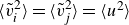 $\langle \tilde {v}^2_{i} \rangle = \langle \tilde {v}^2_{j} \rangle = \langle u^2 \rangle$
. Hence, from (2.35) it follows that
$\langle \tilde {v}^2_{i} \rangle = \langle \tilde {v}^2_{j} \rangle = \langle u^2 \rangle$
. Hence, from (2.35) it follows that
 $\sigma _{\textit{II}}^2=0$
. Hence, not only the contribution of Mechanism I, but the entire IMSC reduces to the formulation of Saffman & Turner (Reference Saffman and Turner1956), (C1), in the limit of
$\sigma _{\textit{II}}^2=0$
. Hence, not only the contribution of Mechanism I, but the entire IMSC reduces to the formulation of Saffman & Turner (Reference Saffman and Turner1956), (C1), in the limit of
 $St=0$
.
$St=0$
.
2.6. Modelling of gravity
So far, the IMSC takes into account the stochastic motion of the collision partners due to the influence of turbulence. However, the presence of gravity introduces a deterministic component to the relative velocity, caused by the difference in the rate of rise or sedimentation of different types of dispersed elements in a polydisperse suspension.
 \begin{equation} \Delta \tilde {w}_{{G}} = \tilde {v}_{{G}i} - \tilde {v}_{{G}j}, \end{equation}
where
 $\tilde {v}_{{G}\alpha }$
is the gravity-induced velocity of a class
$\tilde {v}_{{G}\alpha }$
is the gravity-induced velocity of a class
 $\alpha$
of dispersed elements. Several models in the literature describe the rise and sedimentation velocity of single particles and bubbles. A model for the rise velocity of a single bubble in quiescent flow is given by Rodrigue (Reference Rodrigue2001) reading
$\alpha$
of dispersed elements. Several models in the literature describe the rise and sedimentation velocity of single particles and bubbles. A model for the rise velocity of a single bubble in quiescent flow is given by Rodrigue (Reference Rodrigue2001) reading
 \begin{equation} v_{{G}b}^{{(R)}} = Ve \left ( \frac {d_b^2 \rho _{\!f}}{\sigma _{bf} \nu _{\!f}} \right )^{-1/3}, \end{equation}
where
 $Ve$
is the velocity number defined as
$Ve$
is the velocity number defined as
 \begin{equation} Ve = \frac {Fl/12}{1+0.049Fl^{3/4}}, \end{equation}
with the flow number
 \begin{equation} Fl = g\left ( \frac {d_b^8\rho _{\!f}}{\sigma _{bf}\nu _{\!f}^4} \right )^{1/3}, \end{equation}
where
 $d_b=2r_b$
is the bubble diameter and
$d_b=2r_b$
is the bubble diameter and
 $\sigma _{bf}$
is the surface tension of the bubble. For a single particle in quiescent flow, the model of Nguyen & Schulze (Reference Nguyen and Schulze2004) is used here, reading
$\sigma _{bf}$
is the surface tension of the bubble. For a single particle in quiescent flow, the model of Nguyen & Schulze (Reference Nguyen and Schulze2004) is used here, reading
 \begin{equation} v_{{G}p}^{{(NS)}} = \frac {2 r_p^2 (\rho _p-\rho _{\!f}) g}{9 \nu _{\!f} \rho _{\!f}} \left ( 1 + \frac {Ar_p}{96}(1+0.079Ar_p^{0.749})^{-0.755} \right )^{-1}, \end{equation}
with the Archimedes number
 \begin{equation} Ar_\alpha =\frac {8r_\alpha ^3 g (\rho _\alpha -\rho _{\!f})}{\rho _{\!f} \nu ^2}. \end{equation}
To correct for the influence of swarm effects, the same models by Richardson & Zaki (Reference Richardson and Zaki1954) and Garnier et al. (Reference Garnier, Lance and Marié2002), (2.17), as used in § 2.4.1, are employed here to determine the correction factor
 $c_\epsilon$
, giving
$c_\epsilon$
, giving
 \begin{equation} v_{{G}\alpha } = \begin{cases} v_{{G}b}^{{(R)}}c_{\epsilon b}, \hspace {0.7cm} \alpha =b,\\[5pt] v_{{G}p}^{{(NS)}}c_{\epsilon p}, \hspace {0.5cm} \alpha =p, \end{cases} \end{equation}
for bubbles and particles, respectively. The remarks in § 2.4.1 above concerning a suitable choice of the swarm corrections apply here as well.
Bubble Reynolds number as a function of bubble diameter
 $d_b$
for particle diameters of
$d_b$
for particle diameters of
 $d_p={30}\,{\unicode{x03BC}}\textrm {m}$
(
$d_p={30}\,{\unicode{x03BC}}\textrm {m}$
(![]() ) and
) and
 $d_p={50}\,{\mu } \textrm {m}$
(
$d_p={50}\,{\mu } \textrm {m}$
(![]() ), both with
), both with
 $\epsilon _b={8.8}\,{\%}$
, as obtained in the DNS. The rise velocity according to the models by Rodrigue (Reference Rodrigue2001) (
$\epsilon _b={8.8}\,{\%}$
, as obtained in the DNS. The rise velocity according to the models by Rodrigue (Reference Rodrigue2001) (![]() ) and Clift et al. (Reference Clift, Grace and Weber1978) (
) and Clift et al. (Reference Clift, Grace and Weber1978) (![]() ), both corrected for the presence of a bubble swarm according to Garnier et al. (Reference Garnier, Lance and Marié2002), are shown for reference. The shaded area approximately marks the regime of non-spherical bubbles (from Tiedemann & Fröhlich (Reference Tiedemann and Fröhlich2025)).
), both corrected for the presence of a bubble swarm according to Garnier et al. (Reference Garnier, Lance and Marié2002), are shown for reference. The shaded area approximately marks the regime of non-spherical bubbles (from Tiedemann & Fröhlich (Reference Tiedemann and Fröhlich2025)).

In addition to the validation of these models in the literature (Rodrigue Reference Rodrigue2001; Nguyen & Schulze Reference Nguyen and Schulze2004), a brief comparison with the simulation data is made here. Only the simulations in which gravity is the primary driver of particle and bubble motion are utilised, as in these cases the velocity component due to gravity can be clearly distinguished. Figure 4 shows the bubble Reynolds number as a function of
 $d_b$
for different
$d_b$
for different
 $d_p$
. Obviously, changes in
$d_p$
. Obviously, changes in
 $d_p$
have little influence on the movement of the bubbles for the fine particles considered here. The data are compared with the model by Rodrigue (Reference Rodrigue2001) supplied with the swarm correction of Garnier et al. (Reference Garnier, Lance and Marié2002). The agreement is very good up to a bubble diameter of
$d_p$
have little influence on the movement of the bubbles for the fine particles considered here. The data are compared with the model by Rodrigue (Reference Rodrigue2001) supplied with the swarm correction of Garnier et al. (Reference Garnier, Lance and Marié2002). The agreement is very good up to a bubble diameter of
 $d_b={1.4}\,\textrm{mm}$
. For
$d_b={1.4}\,\textrm{mm}$
. For
 $d_b = {2.4}\,\,\textrm{mm}$
, a discrepancy of
$d_b = {2.4}\,\,\textrm{mm}$
, a discrepancy of
 ${15}\,{\%}$
can be observed between the modelled rise velocity and the simulation result. This particular case, characterised by a bubble Reynolds number
${15}\,{\%}$
can be observed between the modelled rise velocity and the simulation result. This particular case, characterised by a bubble Reynolds number
 $Re=330$
, is situated at the threshold of the assumption of spherical bubbles according to the regime map of Clift et al. (Reference Clift, Grace and Weber1978). While in the simulations rigid bubbles with
$Re=330$
, is situated at the threshold of the assumption of spherical bubbles according to the regime map of Clift et al. (Reference Clift, Grace and Weber1978). While in the simulations rigid bubbles with
 $Eo=0$
are assumed, in reality
$Eo=0$
are assumed, in reality
 $Eo\approx 0.77$
for this case. Overall, this causes a difference from the simulation results and the model by Rodrigue (Reference Rodrigue2001). This data point was included in the figure for further reference. Finally, a comparison is also made with the model of Clift et al. (Reference Clift, Grace and Weber1978) for the bubble rise velocity using the same swarm correction of Garnier et al. (Reference Garnier, Lance and Marié2002). As it provides worse results, it is not used in the IMSC.
$Eo\approx 0.77$
for this case. Overall, this causes a difference from the simulation results and the model by Rodrigue (Reference Rodrigue2001). This data point was included in the figure for further reference. Finally, a comparison is also made with the model of Clift et al. (Reference Clift, Grace and Weber1978) for the bubble rise velocity using the same swarm correction of Garnier et al. (Reference Garnier, Lance and Marié2002). As it provides worse results, it is not used in the IMSC.
Using the decomposition of the relative velocity introduced earlier,
 $w$
is split into a contribution from the motion of the collision partners with the fluid (Mechanism I) and a contribution from the motion of the collision partners relative to the fluid (Mechanism II). As gravity causes a motion relative to the fluid, a combined effect of Mechanism II and gravity,
$w$
is split into a contribution from the motion of the collision partners with the fluid (Mechanism I) and a contribution from the motion of the collision partners relative to the fluid (Mechanism II). As gravity causes a motion relative to the fluid, a combined effect of Mechanism II and gravity,
 $w_{{\textit{II}},\mathrm{G}}$
, is used following a method by Dodin & Elperin (Reference Dodin and Elperin2002). Thus, (2.9) changes to
$w_{{\textit{II}},\mathrm{G}}$
, is used following a method by Dodin & Elperin (Reference Dodin and Elperin2002). Thus, (2.9) changes to
 \begin{equation} w_{r,{\textit{rms}}} =\sqrt {\frac {2}{\pi }\sigma _I^2 + \big\langle w_{{\textit{II}},\mathrm{G}}^2 \big\rangle }. \end{equation}
Similar to the definition of the spherical collision kernel in (1.3), the flux over the collision sphere of radius
 $r_c$
due to
$r_c$
due to
 $w_{{\textit{II}},\mathrm{G}}$
is
$w_{{\textit{II}},\mathrm{G}}$
is
 \begin{equation} F_G = \sqrt {\langle w_{{\textit{II}},\mathrm{G}}^2 \rangle } 4\pi r_c^2 = \int _{0}^{2\pi } \int _{0}^{\pi } r_c^2 \sin (\phi ) \cos (\theta ) \sqrt {w_{{\textit{II}},\mathrm{G},r}^2(\phi ,\theta )}\, \mathrm{d} \phi \mathrm{d} \theta , \end{equation}
where
 $w_{{\textit{II}},\mathrm{G},r}$
is the radial component of
$w_{{\textit{II}},\mathrm{G},r}$
is the radial component of
 $w_{{\textit{II}},\mathrm{G}}$
. Assuming a Gaussian probability distribution for the relative velocity yields
$w_{{\textit{II}},\mathrm{G}}$
. Assuming a Gaussian probability distribution for the relative velocity yields
 \begin{align} \sqrt {\langle w_{{\textit{II}},\mathrm{G}}^2 \rangle } &= \int _{\phi = 0}^{\pi /2} \int _{w=-\infty }^{\infty } \sin (\phi ) (w-\cos (\phi ) \Delta w_{{G}} )\nonumber\\ &\quad\times \frac {1}{\sqrt {2\pi \sigma ^2_{\textit{II}}}} \exp \left ( - \frac {w^2}{2\sigma ^2_{\textit{II}}} \right ) \mathrm{d} w \mathrm{d} \phi , \end{align}
with
 $\Delta w_G=\Delta \tilde {w}_{{G}}$
, defined in (2.38), since the relative velocity is the same in a fixed and a moving frame of reference. This integral is inaccessible for analytical treatment (Abrahamson Reference Abrahamson1975), so that numerical integration must be performed. Suitable limits of integration for
$\Delta w_G=\Delta \tilde {w}_{{G}}$
, defined in (2.38), since the relative velocity is the same in a fixed and a moving frame of reference. This integral is inaccessible for analytical treatment (Abrahamson Reference Abrahamson1975), so that numerical integration must be performed. Suitable limits of integration for
 $w$
are
$w$
are
 $[-3\sigma _{\textit{II}}, 3\sigma _{\textit{II}}]$
, instead of
$[-3\sigma _{\textit{II}}, 3\sigma _{\textit{II}}]$
, instead of
 $[-\infty , \infty ]$
.
$[-\infty , \infty ]$
.
2.7. Fluid disturbance by large bubbles
So far, only collisions between similarly sized collision partners have been considered, such as those involving pairs of bubbles or pairs of particles. It has been assumed that the presence of the collision partners and their interaction with the fluid do not significantly alter the relative velocity between them. However, this assumption is not valid when the collision partners exhibit a substantial disparity in size, as is often the case in flotation. Bubbles significantly alter the fluid field around them and, hence, the radial relative velocity of small particles approaching them. The method discussed in the following can also be employed for pairs of bubbles, pairs of particles or pairs of particles and bubbles of vastly different sizes. The index
 $j$
refers to the larger collision partner, and
$j$
refers to the larger collision partner, and
 $i$
to the smaller partner.
$i$
to the smaller partner.
Schematic of the deflection of a small particle by the flow field modulations around a large bubble (after Nguyen (Reference Nguyen1999)).

The deviation of the particle from its original trajectory and the subsequent change of the radial relative velocity are illustrated in figure 5. The previously combined radial relative velocity for Mechanism II and gravity,
 $w_{{\textit{II}},\mathrm{G}}$
, is taken as the far-field approach velocity
$w_{{\textit{II}},\mathrm{G}}$
, is taken as the far-field approach velocity
 $w_\infty$
(Kostoglou et al. Reference Kostoglou, Karapantsios and Evgenidis2020a
). Nguyen (Reference Nguyen1999) devised a description of the flow field surrounding a bubble. Assuming that the larger collision partner
$w_\infty$
(Kostoglou et al. Reference Kostoglou, Karapantsios and Evgenidis2020a
). Nguyen (Reference Nguyen1999) devised a description of the flow field surrounding a bubble. Assuming that the larger collision partner
 $j$
is a bubble with an immobile bubble surface, the local radial relative velocity at the collision radius
$j$
is a bubble with an immobile bubble surface, the local radial relative velocity at the collision radius
 $w_r$
results in
$w_r$
results in
 \begin{equation} \frac {w_r}{w_\infty } = \frac {2X\cos (\varPhi ) + 3 Y \cos ^2(\varPhi )- Y}{2} \left ( \frac {r_i}{r_{\!j}}\right )^2, \end{equation}
where
 \begin{equation} X = \frac {3}{2}+\frac {9}{32}\frac {{\textit{Re}}_{j}}{1+0.309{\textit{Re}}_{j}^{0.694}},\hspace {0.3cm}Y = \frac {3}{8} \frac {{\textit{Re}}_{j}}{1+0.217{\textit{Re}}_{j}^{0.518}}, \end{equation}
valid for
 $r_i/r_{\!j}\lt (r_i/r_{\!j})_m=0.1$
. The DNS data utilised for subsequent validation suggest that the assumption regarding the independence of collision partners on their relative velocity, due to their coupling with the fluid, holds true for the condition
$r_i/r_{\!j}\lt (r_i/r_{\!j})_m=0.1$
. The DNS data utilised for subsequent validation suggest that the assumption regarding the independence of collision partners on their relative velocity, due to their coupling with the fluid, holds true for the condition
 $r_i/r_{\!j}\gt (r_i/r_{\!j})_n=0.3$
(cf. §§ 3.4.1 and 4.1). To bridge the gap, the following piecewise correction factor
$r_i/r_{\!j}\gt (r_i/r_{\!j})_n=0.3$
(cf. §§ 3.4.1 and 4.1). To bridge the gap, the following piecewise correction factor
 $(w_r/w_\infty )^2$
for
$(w_r/w_\infty )^2$
for
 $\langle w_{{\textit{II}},\mathrm{G}}^2 \rangle$
in (2.45) is introduced:
$\langle w_{{\textit{II}},\mathrm{G}}^2 \rangle$
in (2.45) is introduced:
 \begin{align} \left ( \frac {w_r}{w_\infty } \right )^2\! &=\! \begin{cases} \left ( \dfrac {1}{4} Y\left (\dfrac {r_i}{r_{\!j}}\right )^2 \right )^2, &\mathrm{if}\,r_i/r_{\!j}\leqslant (r_i/r_{\!j})_m, \\ \left ( \!Z + \dfrac {1-Z}{(r_i/r_{\!j})_n-(r_i/r_{\!j})_m}\left (\dfrac {r_i}{r_{\!j}}\! - (r_i/r_{\!j})_m\!\right )\! \right )^2\!, &\mathrm{if}\,(r_i/r_{\!j})_m\!\lt r_i/r_{\!j}\leqslant (r_i/r_{\!j})_n, \\ 1, &\mathrm{else}, \end{cases} \end{align}
where
 \begin{equation} Z = \left (\left (\frac {r_i}{r_{\!j}}\right )_m\right )^2\frac {1}{4} Y= 0.0025 \ Y. \end{equation}
The final expression of the radial relative velocity, then, is
 \begin{equation} w_{r,{\textit{rms}}} = \sqrt {\frac {2}{\pi }\sigma _I^2 + \left\langle w_{{\textit{II}},\mathrm{G}}^2\right\rangle \left ( \frac {w_r}{w_\infty }\right )^2}. \end{equation}
Figure 6 exemplarily illustrates the behaviour of the IMSC using this correction for varying
 $r_p/r_b$
. To this end, all statistical quantities were taken over from G-1-30 defined in table 5 below and
$r_p/r_b$
. To this end, all statistical quantities were taken over from G-1-30 defined in table 5 below and
 $r_p$
was changed. The resulting data illustrate the impact of the size ratio, as accounted for by the model.
$r_p$
was changed. The resulting data illustrate the impact of the size ratio, as accounted for by the model.
Exemplary alteration of the relative velocity due to a modulated flow field as modelled by the IMSC. Input parameters (such as
 $k$
,
$k$
,
 $\varepsilon$
,
$\varepsilon$
,
 $\epsilon _p$
,
$\epsilon _p$
,
 $\epsilon _g$
, etc.) correspond to case G-1-30 in table 5. Only
$\epsilon _g$
, etc.) correspond to case G-1-30 in table 5. Only
 $r_p$
was varied.
$r_p$
was varied.

2.8. Summary of the model
Including all these components, the IMSC is a model for the collisions between particles and bubbles, pairs of particles and pairs of bubbles. A guideline for the necessary steps of its implementation is shown in figure 1 above to be read from left to right.
The following input parameters are required for the IMSC. For the fluid: turbulent kinetic energy
 $k$
, turbulent dissipation rate
$k$
, turbulent dissipation rate
 $\varepsilon$
, fluid density
$\varepsilon$
, fluid density
 $\rho _{\!f}$
, kinematic viscosity
$\rho _{\!f}$
, kinematic viscosity
 $\nu _{\!f}$
. For each of the two dispersed phases
$\nu _{\!f}$
. For each of the two dispersed phases
 $\alpha =i,j=p,b$
, i.e. particles or bubbles: radius of the elements
$\alpha =i,j=p,b$
, i.e. particles or bubbles: radius of the elements
 $r_\alpha$
, density of the elements
$r_\alpha$
, density of the elements
 $\rho _\alpha$
, volume fraction of the phase
$\rho _\alpha$
, volume fraction of the phase
 $\epsilon _\alpha$
, Reynolds number
$\epsilon _\alpha$
, Reynolds number
 ${\textit{Re}}_\alpha$
. Finally, the surface tension
${\textit{Re}}_\alpha$
. Finally, the surface tension
 $\sigma _{bf}$
is needed to model the rise velocity of the bubbles.
$\sigma _{bf}$
is needed to model the rise velocity of the bubbles.
Based on these input parameters, the corrections for the swarm effects and for the deviation from Stokes drag can be determined according to (2.15) and (2.17). The next step is to determine the individual contributions for Mechanism I and Mechanism II. The contribution of Mechanism I is given in (2.34), using the piecewise definition of the fluid structure function (2.33), the velocity correlations in (2.27), (2.28) and the parabolic exponential autocorrelation function of Williams (Reference Williams1980) in (2.20). The combined effects of Mechanism II and gravity are described by the integral in (2.47). This integral must be solved numerically. Suitable limits of integration for
 $w$
are
$w$
are
 $[-3\sigma _{\textit{II}}, 3\sigma _{\textit{II}}]$
. If there is a significant size difference between particles and bubbles, the disturbance of the flow field due to the presence of the bubble is accounted for in particle–bubble collisions. The correction factor is given in (2.50), where the larger collision partner, usually the bubble, is assumed to be collision partner
$[-3\sigma _{\textit{II}}, 3\sigma _{\textit{II}}]$
. If there is a significant size difference between particles and bubbles, the disturbance of the flow field due to the presence of the bubble is accounted for in particle–bubble collisions. The correction factor is given in (2.50), where the larger collision partner, usually the bubble, is assumed to be collision partner
 $j$
and the smaller one collision partner
$j$
and the smaller one collision partner
 $i$
. The individual components of the modelled radial relative velocity are then combined in (2.52), and the collision kernel is determined based on the spherical formulation (1.4). A concise summary of all the equations needed to implement the model is given in table 2 of Appendix A with a clear distinction which model parts were taken from existing literature and which parts were newly created.
$i$
. The individual components of the modelled radial relative velocity are then combined in (2.52), and the collision kernel is determined based on the spherical formulation (1.4). A concise summary of all the equations needed to implement the model is given in table 2 of Appendix A with a clear distinction which model parts were taken from existing literature and which parts were newly created.
While the above-mentioned input parameters are those which are at least required for the IMSC, depending on the large-scale model in which the IMSC is employed, a variety of other parameters might be available. For example, some Euler–Euler models also solve for granular temperatures or velocity variances of the collision partners (Gevrin, Masbernat & Simonin Reference Gevrin, Masbernat and Simonin2008; Yang, Padding & Kuipers Reference Yang, Padding and Kuipers2016; Liu et al. Reference Liu, He, Chen, Li, Zhao, Xu and Wang2025). This information can be used in several instances in the IMSC. If a mean settling or rise velocity of the collision partners is known, the submodels used to predict
 $v_{G\alpha }$
can be replaced by this information. The variance for Mechanism II is based on the variance of the slip velocity distribution of both collision partners. If this slip velocity distribution is known from the underlying Euler–Euler framework, it can be readily employed in (2.35). The same holds analogously for Mechanism I.
$v_{G\alpha }$
can be replaced by this information. The variance for Mechanism II is based on the variance of the slip velocity distribution of both collision partners. If this slip velocity distribution is known from the underlying Euler–Euler framework, it can be readily employed in (2.35). The same holds analogously for Mechanism I.
The IMSC combines existing modelling approaches and newly designed ones into a new collision model. The decomposition of the relative velocity approach by Yuu (Reference Yuu1984) was further developed to be based on the spherical collision kernel and to include a combined contribution of Mechanism II and gravity. Furthermore, the correction to account for the size difference of the particles and the bubbles was introduced into this approach. A transition was implemented to account for a variety of particle and bubble size differences. Within the description of Mechanism I, submodels for the fluid autocorrelation function were selected. Importantly, the entire model was validated by data from corresponding DNS. Based on the DNS data, a fluid structure function with a cutoff length scale was implemented. Appropriate models for the drag correction, swarm correction and the rise and settling velocity due to gravity were chosen. Lastly, the selection of the individual submodels, such as the drag correction, swarm correction, as well as the models for the rise and settling velocity of the particles and bubbles, was made based on resolved DNS data.
In order to model the overall flotation process, the IMSC has to be combined with other models covering further subprocesses such as attachment, detachment and entrainment. Using those models, the intricate effects such as reagent usage, surface properties and hydrophobicity could be taken into account.
3. Validation with DNS for bubbles and fine particles
3.1. Numerical set-up and computational method of DNS
An important issue with earlier models for the collision frequency is their inaccuracy in predicting collision rates obtained from DNS (Chan et al. Reference Chan, Ng and Krug2023; Tiedemann & Fröhlich Reference Tiedemann and Fröhlich2024, Reference Tiedemann and Fröhlich2025). Hence, this section and the subsequent § 4 focus on validating the IMSC with well-controlled numerical simulations and compare it with a range of other models. Beyond validating the model as a whole, the data are used to assess fundamental modelling assumptions and to provide hints for the selection of appropriate models of specific subprocesses.
A comprehensive description of these simulations and the results obtained can be found in Tiedemann & Fröhlich (Reference Tiedemann and Fröhlich2024, Reference Tiedemann and Fröhlich2025). The majority of the simulations focused on the separation and concentration zones of the flotation cell, where low turbulence intensity levels prevail (Tiedemann & Fröhlich Reference Tiedemann and Fröhlich2025). In this situation, the main driver of particle as well as bubble motion is gravity acting in the vertical
 $y$
-direction. Additionally, a case exhibiting medium turbulence levels was obtained using the same method with the additional forcing of the background flow to emulate the effects of the rotor and stator in mechanical flotation cells (Tiedemann & Fröhlich Reference Tiedemann and Fröhlich2024). This was devised according to Chouippe & Uhlmann (Reference Chouippe and Uhlmann2015), who employed the method of Eswaran & Pope (Reference Eswaran and Pope1988). Between the different simulation cases, the physical parameters influencing the bubble collision process were varied, such as the bubble diameter
$y$
-direction. Additionally, a case exhibiting medium turbulence levels was obtained using the same method with the additional forcing of the background flow to emulate the effects of the rotor and stator in mechanical flotation cells (Tiedemann & Fröhlich Reference Tiedemann and Fröhlich2024). This was devised according to Chouippe & Uhlmann (Reference Chouippe and Uhlmann2015), who employed the method of Eswaran & Pope (Reference Eswaran and Pope1988). Between the different simulation cases, the physical parameters influencing the bubble collision process were varied, such as the bubble diameter
 $d_b$
, the particle diameter
$d_b$
, the particle diameter
 $d_p$
, particle density
$d_p$
, particle density
 $\rho _p$
, as well as the gas hold-up
$\rho _p$
, as well as the gas hold-up
 $\epsilon _g$
(i.e. the bubble volume fraction) and the particle volume fraction
$\epsilon _g$
(i.e. the bubble volume fraction) and the particle volume fraction
 $\epsilon _p$
. The parameters were chosen to cover the range of realistic flotation conditions (Deglon et al. Reference Deglon, Egya-mensah and Franzidis2000; Tabosa et al. Reference Tabosa, Runge and Holtham2016; Norori-McCormac et al. Reference Norori-McCormac, Brito-Parada, Hadler, Cole and Cilliers2017; Hadler & Cilliers Reference Hadler and Cilliers2019; Ran et al. Reference Ran, Qiu, Hu, Liu, Song and Yao2019; Mesa, Morrison & Brito-Parada Reference Mesa, Morrison and Brito-Parada2020; Ostadrahimi et al. Reference Ostadrahimi, Farrokhpay, Gharibi and Dehghani2020). Furthermore, a case emulating particle-laden bubbles, i.e. with higher bubble density, was simulated.
$\epsilon _p$
. The parameters were chosen to cover the range of realistic flotation conditions (Deglon et al. Reference Deglon, Egya-mensah and Franzidis2000; Tabosa et al. Reference Tabosa, Runge and Holtham2016; Norori-McCormac et al. Reference Norori-McCormac, Brito-Parada, Hadler, Cole and Cilliers2017; Hadler & Cilliers Reference Hadler and Cilliers2019; Ran et al. Reference Ran, Qiu, Hu, Liu, Song and Yao2019; Mesa, Morrison & Brito-Parada Reference Mesa, Morrison and Brito-Parada2020; Ostadrahimi et al. Reference Ostadrahimi, Farrokhpay, Gharibi and Dehghani2020). Furthermore, a case emulating particle-laden bubbles, i.e. with higher bubble density, was simulated.
The simulation cases are labelled as follows. First, a letter to indicate the driving mechanism, with G for gravity-driven alone and RXX for gravity and turbulent background forcing as the driver of the flow. In the latter case, RXX represents the Taylor Reynolds number of the single-phase flow obtained by the forcing. The second and third items in the label indicate the bubble diameter and the particle diameter, respectively. Other parameters different from the reference case G-1-30 are denoted in the last part. The simulation data obtained over a wide range of flotation conditions enable a comprehensive comparison of the IMSC with other models. The complete list of cases with the main physical parameters can be found in table 5.
3.2. Fluid isotropy
A main assumption made for the IMSC in § 2.2 is the presence of homogeneous and isotropic turbulence. The adequacy of this assumption is validated using the present DNS data. The anisotropy of the fluid velocities is fully given by the normalised anisotropy tensor as stated by Pope (Reference Pope2000). Only regarding the main diagonal elements of the normalised anisotropy tensor, disregarding the isotropic stresses and using the fact that the fluid velocity fluctuations in
 $x$
- and
$x$
- and
 $z$
-perpendicular to gravity exhibit almost no difference, the remaining entry of the normalised anisotropy tensor is (Tiedemann & Fröhlich Reference Tiedemann and Fröhlich2024, Reference Tiedemann and Fröhlich2025)
$z$
-perpendicular to gravity exhibit almost no difference, the remaining entry of the normalised anisotropy tensor is (Tiedemann & Fröhlich Reference Tiedemann and Fröhlich2024, Reference Tiedemann and Fröhlich2025)
 \begin{equation} a_a = \sqrt {\frac {\langle u^\prime _{y} u^\prime _{y} \rangle }{\langle u^\prime _{x} u^\prime _{x} \rangle }}. \end{equation}
In this anisotropy factor, the fluid velocity fluctuations in the direction of gravity,
 $u^\prime _{f,y}$
, are related to the fluid velocity fluctuations perpendicular to it,
$u^\prime _{f,y}$
, are related to the fluid velocity fluctuations perpendicular to it,
 $u^\prime _{f,x}$
.
$u^\prime _{f,x}$
.
For the gravity-driven cases with a bubble diameter of
 $d_b={1}\,\,\textrm{mm}$
, the anisotropy factor is
$d_b={1}\,\,\textrm{mm}$
, the anisotropy factor is
 $a_a \approx 2.4$
. For larger bubbles of
$a_a \approx 2.4$
. For larger bubbles of
 $d_b={2.4}\,\,\textrm{mm}$
, creating a higher turbulence intensity, it reduces to
$d_b={2.4}\,\,\textrm{mm}$
, creating a higher turbulence intensity, it reduces to
 $a_a \approx 1.9$
. In the moderately turbulent case R53-1-30, the anisotropy factor is only
$a_a \approx 1.9$
. In the moderately turbulent case R53-1-30, the anisotropy factor is only
 $a_a=1.05$
, indicating very weak anisotropy. This is attributable to the larger unsteady sideward components of the bubble motion exhibited, resulting from the turbulent agitation. As a result, the underlying homogeneous and isotropic forced turbulence is overshadowing the bubble-induced turbulence, thus reducing the overall anisotropy. Hence, for this case as well as similar cases from the literature (Chan et al. Reference Chan, Ng and Krug2023, Reference Chan, L. and Krug2025), the assumption of isotropic turbulence made in the IMSC corresponds with the simulation data.
$a_a=1.05$
, indicating very weak anisotropy. This is attributable to the larger unsteady sideward components of the bubble motion exhibited, resulting from the turbulent agitation. As a result, the underlying homogeneous and isotropic forced turbulence is overshadowing the bubble-induced turbulence, thus reducing the overall anisotropy. Hence, for this case as well as similar cases from the literature (Chan et al. Reference Chan, Ng and Krug2023, Reference Chan, L. and Krug2025), the assumption of isotropic turbulence made in the IMSC corresponds with the simulation data.
3.3. Velocity distribution
An assumption of the IMSC made in § 2.3 and in other collision frequency models is that the velocity distribution of particles and bubbles is Gaussian. Although it is well known that this is not entirely true, the literature suggests that a Gaussian distribution of particle and bubble velocity can be a good approximation for the first two moments of the probability distribution (Wang et al. Reference Wang, Chen, Brasseur and Wyngaard1996). The validity of this assumption and the modelled velocity distributions is now validated by the data published in Tiedemann & Fröhlich (Reference Tiedemann and Fröhlich2024, Reference Tiedemann and Fröhlich2025). Under the conditions addressed there, the Kolmogorov length scale is of the order of the particle diameter, while the bubble diameter is larger than the Taylor length scale for all cases. In this situation, the model sets
 $S_{\ell \ell }^{\textit{(IMSC)}}(r_p)\gt 0$
and
$S_{\ell \ell }^{\textit{(IMSC)}}(r_p)\gt 0$
and
 $S_{\ell \ell }^{\textit{(IMSC)}}(r_b)=0$
, according to (2.33).
$S_{\ell \ell }^{\textit{(IMSC)}}(r_b)=0$
, according to (2.33).
Probability density function of particle and bubble velocity for simulation cases R53-1-30 and G-1-30, as defined in table 5, in comparison with several models. (a) Particle velocity for G-1-30, (b) bubble velocity for G-1-30, (c) particle velocity for R53-1-30, (d) bubble velocity for R53-1-30. With
 $\alpha =b,p$
the curves show
$\alpha =b,p$
the curves show ![]()
 $v_{\alpha x}$
from DNS,
$v_{\alpha x}$
from DNS, ![]()
 $v_{\alpha y}$
from DNS,
$v_{\alpha y}$
from DNS, ![]()
 $v_\alpha$
with the ISMC,
$v_\alpha$
with the ISMC, ![]()
 $v_\alpha$
with the model of Abrahamson (Reference Abrahamson1975),
$v_\alpha$
with the model of Abrahamson (Reference Abrahamson1975), ![]()
 $v_\alpha$
with the model of Kruis & Kusters (Reference Kruis and Kusters1997),
$v_\alpha$
with the model of Kruis & Kusters (Reference Kruis and Kusters1997), ![]()
 $v_\alpha$
with the model of Zaichik et al. (Reference Zaichik, Simonin and Alipchenkov2010). The vertical line denotes
$v_\alpha$
with the model of Zaichik et al. (Reference Zaichik, Simonin and Alipchenkov2010). The vertical line denotes
 $v_\alpha =0$
. In (a) the curves of DNS and IMSC are on top of each other.
$v_\alpha =0$
. In (a) the curves of DNS and IMSC are on top of each other.

Figure 7 shows the probability density function of the particle and bubble velocities for the gravity-driven case G-1-30 and the turbulence-driven case R53-1-30. Detailed information on the first four moments of the particle and bubble velocity distribution for all cases is provided in tables 3 and 4 of Appendix B. The corresponding IMSC results are also given for comparison.
For the gravity-driven case G-1-30, the mean velocity perpendicular to gravity is close to zero for both particles and bubbles. Perpendicular to gravity, the skewness and kurtosis of the bubble velocity distribution are close to the values of a Gaussian probability distribution with a skewness of zero and a kurtosis of three. While the particle velocity distribution in these directions is also only barely skewed, it has positive excess kurtosis. In the direction of gravity, the mean velocity of the bubbles is positive and the mean velocity of the particles is negative, indicating their rising and settling, respectively. Furthermore, the variance of the velocity distribution obtained from the simulation in the direction of gravity is higher than those perpendicular to gravity, indicating more velocity fluctuations of particles and bubbles in this direction. The skewness and kurtosis of the bubble velocity are still close to those of a Gaussian distribution. However, the particle velocity distribution in the direction of gravity is negatively skewed. This is due to the fact that in cases where gravity is the main driving force, the motion of the particle in the vertical direction is strongly influenced by the wakes of the bubbles. Also, in the direction of gravity, the particle velocity distribution has positive excess kurtosis.
For the turbulence-driven case R53-1-30, the mean of both the particle and the bubble velocity distribution is close to zero in all spatial directions. The offset in the direction of gravity is small compared with the gravity-driven cases, since the isotropic turbulence-induced motion of particles and bubbles dominates over the anisotropic gravity-induced motion. The third and fourth moments of both velocity distributions are well matched by a Gaussian probability distribution in all directions. As highlighted above, the data show that for the purpose of modelling, where only the first two moments of the velocity distribution are needed, a Gaussian probability distribution is a suitable choice.
Figure 7 also compares the velocity distributions with different models from the literature. It should be noted that only those models capable of independently modelling the velocity distributions of the collision partners are shown here. The velocities perpendicular to the direction of gravity are the focus of this analysis. For case R53-1-30, the particle velocity distribution is almost exactly matched by the IMSC. The models by Abrahamson (Reference Abrahamson1975), Kruis & Kusters (Reference Kruis and Kusters1997) and Zaichik et al. (Reference Zaichik, Simonin and Alipchenkov2010) provide similar predictions also closely matching the DNS data. For case G-1-30, the particle velocity distribution is well matched by the IMSC and the models of Kruis and Kusters, and Zaichik. The model of Abrahamson (Reference Abrahamson1975) does not agree with the particle velocity distribution, as it was designed for particles with
 $St\rightarrow \infty$
and no gravity, which does not align with the conditions of the simulations.
$St\rightarrow \infty$
and no gravity, which does not align with the conditions of the simulations.
The bubble velocity distribution for both cases, G-1-30 and R53-1-30, is well matched by the IMSC and the model of Kruis & Kusters (Reference Kruis and Kusters1997), which provide similar predictions. The model of Abrahamson (Reference Abrahamson1975) captures only the bubble velocity distribution for case G-1-30. Conversely, the bubble velocity distribution is not well predicted by the model of Zaichik et al. (Reference Zaichik, Simonin and Alipchenkov2010) in both cases. For case R53-1-30, it provides a prediction close to the model of Abrahamson (Reference Abrahamson1975). A more detailed discussion of the models and their match to the simulation data can be found in the following sections.
3.4. Collision kernel
3.4.1. Particle–bubble collision kernel
Due to its direct influence on the flotation performance and recovery, an accurate prediction of the particle–bubble collision kernel is of high interest. Figure 8 provides a comparison of the results obtained from the DNS with those from the IMSC and different models for the collision kernel from the literature. The input parameters for the models were the same as for the simulations listed in table 5 and described in § 3.1. The values for
 $k$
,
$k$
,
 $\varepsilon$
and
$\varepsilon$
and
 ${\textit{Re}}_\alpha$
were taken from the DNS results. The line connecting the data points is for orientation only and does not imply a physical connection. In the simulations, several parameters like the turbulence forcing, the bubble diameter or the particle diameter were varied. On this basis, conclusions can be drawn which effects are well captured by the models.
${\textit{Re}}_\alpha$
were taken from the DNS results. The line connecting the data points is for orientation only and does not imply a physical connection. In the simulations, several parameters like the turbulence forcing, the bubble diameter or the particle diameter were varied. On this basis, conclusions can be drawn which effects are well captured by the models.
Comparison of non-dimensional bubble–particle collision kernel obtained from DNS and various models. The cases are defined in table 5. Here ![]() DNS,
DNS, ![]() IMSC,
IMSC, ![]() Abrahamson (Reference Abrahamson1975),
Abrahamson (Reference Abrahamson1975), ![]() Kostoglou et al. (Reference Kostoglou, Karapantsios and Evgenidis2020a
),
Kostoglou et al. (Reference Kostoglou, Karapantsios and Evgenidis2020a
), ![]() Kruis & Kusters (Reference Kruis and Kusters1997),
Kruis & Kusters (Reference Kruis and Kusters1997), ![]() Saffman & Turner (Reference Saffman and Turner1956),
Saffman & Turner (Reference Saffman and Turner1956), ![]() Dodin & Elperin (Reference Dodin and Elperin2002),
Dodin & Elperin (Reference Dodin and Elperin2002), ![]() Zaichik et al. (Reference Zaichik, Simonin and Alipchenkov2010),
Zaichik et al. (Reference Zaichik, Simonin and Alipchenkov2010), ![]() Ngo-Cong et al. (Reference Ngo-Cong, Nguyen and Tran-Cong2018).
Ngo-Cong et al. (Reference Ngo-Cong, Nguyen and Tran-Cong2018).

The models of Saffman & Turner (Reference Saffman and Turner1956), Abrahamson (Reference Abrahamson1975), Zaichik et al. (Reference Zaichik, Simonin and Alipchenkov2010) and Ngo-Cong et al. (Reference Ngo-Cong, Nguyen and Tran-Cong2018) significantly overpredict the simulation results by almost two orders of magnitude. All these models were designed for collision partners of similar size, do not take into account the changes in the flow field in the vicinity of the bubble, and omit the influence of gravity. In particular, the models of Saffman & Turner (Reference Saffman and Turner1956) and Abrahamson (Reference Abrahamson1975) are based on the limiting cases for
 ${\textit{St}}_\alpha \rightarrow 0$
and
${\textit{St}}_\alpha \rightarrow 0$
and
 ${\textit{St}}_\alpha \rightarrow \infty$
, respectively, without the influence of gravity. Therefore, the underlying modelling assumptions do not match the conditions in the flotation and those present in the simulation. Dodin & Elperin (Reference Dodin and Elperin2002) started from the formulation of Saffman & Turner (Reference Saffman and Turner1956) and incorporated the effect of gravity. Using this formulation, significantly better results are obtained. Their model, when compared with that of Saffman & Turner (Reference Saffman and Turner1956), shows that the combined influence of turbulence and gravity results in a lower collision kernel than would be found in a purely turbulent environment. The deviations observed with the model by Zaichik can be attributed to an overestimation of the variance in the bubble velocity.
${\textit{St}}_\alpha \rightarrow \infty$
, respectively, without the influence of gravity. Therefore, the underlying modelling assumptions do not match the conditions in the flotation and those present in the simulation. Dodin & Elperin (Reference Dodin and Elperin2002) started from the formulation of Saffman & Turner (Reference Saffman and Turner1956) and incorporated the effect of gravity. Using this formulation, significantly better results are obtained. Their model, when compared with that of Saffman & Turner (Reference Saffman and Turner1956), shows that the combined influence of turbulence and gravity results in a lower collision kernel than would be found in a purely turbulent environment. The deviations observed with the model by Zaichik can be attributed to an overestimation of the variance in the bubble velocity.
The models incorporating the effects of gravity, such as those of Kostoglou et al. (Reference Kostoglou, Karapantsios and Evgenidis2020a ), Kruis & Kusters (Reference Kruis and Kusters1997), Dodin & Elperin (Reference Dodin and Elperin2002) as well as the IMSC, provide collision kernels of the same order of magnitude as the DNS data, with the IMSC yielding the best overall fit to the simulation data. The model of Kostoglou et al. (Reference Kostoglou, Karapantsios and Evgenidis2020a ) was developed specifically for the case of fine particles, also including the flow distortion due to the bubble. Hence, its good match is not surprising. However, different models for the bubble and particle terminal velocity, drag modification and differences in the fluid structure function make the IMSC provide a better fit. The Kruis and Kusters model is largely in agreement with the Kostoglou model. However, as previously mentioned, it has an inconsistent use of reference frames and employs the cylindrical collision kernel. This prevents it from being generally applicable.
While many cases are well predicted by the IMSC, the increase in collision frequency with increasing particle density is not well represented (case G-1-30-rp6k). This finding is consistent with the other models, which also demonstrate only a marginal increase over their baseline for the case G-1-30. One potential explanation for this could be a more uneven distribution of collision angles along the bubble circumference for gravitationally driven bubble motion (Tiedemann & Fröhlich Reference Tiedemann and Fröhlich2025).
Case G-1-30-rb25 emulates a loaded bubble with a large portion of the bubble surface area covered with particles. This was obtained by using a higher bubble density. In particular, the Kostoglou model and the IMSC include submodels for the bubble rise velocity based on unladen bubbles without
 $\rho _b$
as input parameter. However, as the bubble density is still low compared with the fluid density, only a little difference in bubble motion and collision behaviour was observed in the DNS (Tiedemann & Fröhlich Reference Tiedemann and Fröhlich2025). Hence, the model by Kostoglou and the IMSC are still able to accurately predict the respective collision kernel.
$\rho _b$
as input parameter. However, as the bubble density is still low compared with the fluid density, only a little difference in bubble motion and collision behaviour was observed in the DNS (Tiedemann & Fröhlich Reference Tiedemann and Fröhlich2025). Hence, the model by Kostoglou and the IMSC are still able to accurately predict the respective collision kernel.
Most other cases with
 $d_b={1}\,\textrm{mm}$
or
$d_b={1}\,\textrm{mm}$
or
 $d_b={0.6}\,\textrm{mm}$
are well matched by the IMSC. The largest discrepancies are noticed for cases G-1.4-30 and G-2.4-50. These cases exhibit the most pronounced size disparity between particles and bubbles within this study. For all cases with
$d_b={0.6}\,\textrm{mm}$
are well matched by the IMSC. The largest discrepancies are noticed for cases G-1.4-30 and G-2.4-50. These cases exhibit the most pronounced size disparity between particles and bubbles within this study. For all cases with
 $d_b={2.4}\,\textrm{mm}$
the bubble rise velocity obtained from the simulations and the ones resulting from the employed submodel by Rodrigue (Reference Rodrigue2001) differ as shown in figure 4 and discussed in § 2.6 above. Furthermore, the slight onset of particle clustering was observed in (Tiedemann & Fröhlich Reference Tiedemann and Fröhlich2025), which may have implications for the particle–bubble collision kernel, not captured by any model (Chan et al. Reference Chan, Ng and Krug2023).
$d_b={2.4}\,\textrm{mm}$
the bubble rise velocity obtained from the simulations and the ones resulting from the employed submodel by Rodrigue (Reference Rodrigue2001) differ as shown in figure 4 and discussed in § 2.6 above. Furthermore, the slight onset of particle clustering was observed in (Tiedemann & Fröhlich Reference Tiedemann and Fröhlich2025), which may have implications for the particle–bubble collision kernel, not captured by any model (Chan et al. Reference Chan, Ng and Krug2023).
3.4.2. Particle–particle collision kernel
In addition to the important particle–bubble collision kernel, also collisions between pairs of particles and pairs of bubbles take place in a flotation cell. In figure 9 the particle–particle collision kernel obtained from the DNS in Tiedemann & Fröhlich (Reference Tiedemann and Fröhlich2024, Reference Tiedemann and Fröhlich2025) is compared with the results of the IMSC and the models of Saffman & Turner (Reference Saffman and Turner1956), Kruis & Kusters (Reference Kruis and Kusters1997) and Zaichik et al. (Reference Zaichik, Simonin and Alipchenkov2010). Note the significantly narrower range of the vertical axis compared with the other graphs reporting collision kernels. Models that assume coarse particles with
 ${\textit{St}}_p\rightarrow \infty$
or that assume a significant size difference between the collision partners such as those of Abrahamson (Reference Abrahamson1975) and Kostoglou et al. (Reference Kostoglou, Karapantsios and Evgenidis2020a
), are not included, because the assumptions in these models are very different from the situation to be described resulting in large discrepancies with the simulation results. All models retained are very close to the simulation results, with the IMSC and the model of Zaichik almost reducing to the limiting case of Saffman & Turner (Reference Saffman and Turner1956). The errors of the predictions for
${\textit{St}}_p\rightarrow \infty$
or that assume a significant size difference between the collision partners such as those of Abrahamson (Reference Abrahamson1975) and Kostoglou et al. (Reference Kostoglou, Karapantsios and Evgenidis2020a
), are not included, because the assumptions in these models are very different from the situation to be described resulting in large discrepancies with the simulation results. All models retained are very close to the simulation results, with the IMSC and the model of Zaichik almost reducing to the limiting case of Saffman & Turner (Reference Saffman and Turner1956). The errors of the predictions for
 $\varGamma _{pp}$
are comparatively small when evaluated against the errors obtained for the other collision kernels. This is to be expected, since the particles in the DNS are mostly of very low Stokes numbers and
$\varGamma _{pp}$
are comparatively small when evaluated against the errors obtained for the other collision kernels. This is to be expected, since the particles in the DNS are mostly of very low Stokes numbers and
 $Re\lt 1$
, thus matching the respective assumptions.
$Re\lt 1$
, thus matching the respective assumptions.
Comparison of non-dimensional particle–particle collision kernel obtained from DNS and various models. The cases are defined in table 5. Here ![]() DNS,
DNS, ![]() IMSC,
IMSC, ![]() Kruis & Kusters (Reference Kruis and Kusters1997),
Kruis & Kusters (Reference Kruis and Kusters1997), ![]() Saffman & Turner (Reference Saffman and Turner1956),
Saffman & Turner (Reference Saffman and Turner1956), ![]() Zaichik et al. (Reference Zaichik, Simonin and Alipchenkov2010). Data of IMSC and Saffman & Turner (Reference Saffman and Turner1956) are on top of each other.
Zaichik et al. (Reference Zaichik, Simonin and Alipchenkov2010). Data of IMSC and Saffman & Turner (Reference Saffman and Turner1956) are on top of each other.

The collision kernels obtained by the DNS fluctuate between cases, which is not properly captured by the models. The movement of particles in the simulation is found to be strongly influenced by the local flow field. Particularly in the vicinity of the bubbles and in regions of high shear the particle motion increases in magnitude and becomes anisotropic. These conditions have a significant impact on the collision kernel. However, they are not captured by the models, which, instead, assume a constant turbulence intensity over the entire subdomain considered.
The largest differences exist for the cases with
 $d_b={2.4}\,\textrm{mm}$
and R53-1-30. These cases have the largest differences in the local fluid velocity fluctuations compared with the average ones (Tiedemann & Fröhlich Reference Tiedemann and Fröhlich2024, Reference Tiedemann and Fröhlich2025). Furthermore, the particle Stokes numbers are highest for these cases. Thus, there is a slight beginning of particle accumulation in certain regions of the flow (Tiedemann & Fröhlich Reference Tiedemann and Fröhlich2024, Reference Tiedemann and Fröhlich2025). This particle clustering has been shown to increase the rate of particle–particle collisions (Voßkuhle et al. Reference Voßkuhle, Pumir, Lévêque and Wilkinson2014; Ireland, Bragg & Collins Reference Ireland, Bragg and Collins2016). While the majority of models predict collision kernels that align closely with the DNS data and the limiting case of Saffman & Turner (Reference Saffman and Turner1956), the collision kernels predicted by the Kruis and Kusters model are found to be inadequate. This finding agrees with the earlier analyses by Wang et al. (Reference Wang, Wexler and Zhou1998) who showed that the cylindrical collision kernel used is not suitable in this situation.
$d_b={2.4}\,\textrm{mm}$
and R53-1-30. These cases have the largest differences in the local fluid velocity fluctuations compared with the average ones (Tiedemann & Fröhlich Reference Tiedemann and Fröhlich2024, Reference Tiedemann and Fröhlich2025). Furthermore, the particle Stokes numbers are highest for these cases. Thus, there is a slight beginning of particle accumulation in certain regions of the flow (Tiedemann & Fröhlich Reference Tiedemann and Fröhlich2024, Reference Tiedemann and Fröhlich2025). This particle clustering has been shown to increase the rate of particle–particle collisions (Voßkuhle et al. Reference Voßkuhle, Pumir, Lévêque and Wilkinson2014; Ireland, Bragg & Collins Reference Ireland, Bragg and Collins2016). While the majority of models predict collision kernels that align closely with the DNS data and the limiting case of Saffman & Turner (Reference Saffman and Turner1956), the collision kernels predicted by the Kruis and Kusters model are found to be inadequate. This finding agrees with the earlier analyses by Wang et al. (Reference Wang, Wexler and Zhou1998) who showed that the cylindrical collision kernel used is not suitable in this situation.
3.4.3. Bubble–bubble collision kernel
The third type of collisions is constituted by bubble–bubble collisions. In figure 10, the collision kernels obtained in the DNS are compared with the IMSC and other models. Comparisons are made with the models of Saffman & Turner (Reference Saffman and Turner1956), Zaichik et al. (Reference Zaichik, Simonin and Alipchenkov2010) and Kruis & Kusters (Reference Kruis and Kusters1997). The model by Kostoglou et al. (Reference Kostoglou, Karapantsios and Evgenidis2020a
) is specifically designed for the collisions of fine particles with bubbles, hence not appropriate for equal-sized bubbles. The model by Abrahamson (Reference Abrahamson1975) significantly underpredicts
 $\varGamma _{bb}$
, as it assumes point particles with
$\varGamma _{bb}$
, as it assumes point particles with
 ${\textit{St}}_p\rightarrow \infty$
not matched by the bubbles. Hence, neither of the two is shown here. The model by Dodin & Elperin (Reference Dodin and Elperin2002) is not shown, as the incorporation of gravitational effects into the model of Saffman & Turner (Reference Saffman and Turner1956) has no added benefit for collision partners of the same class,
${\textit{St}}_p\rightarrow \infty$
not matched by the bubbles. Hence, neither of the two is shown here. The model by Dodin & Elperin (Reference Dodin and Elperin2002) is not shown, as the incorporation of gravitational effects into the model of Saffman & Turner (Reference Saffman and Turner1956) has no added benefit for collision partners of the same class,
 $i=j$
, as no relative velocity due to gravitational settling is obtained.
$i=j$
, as no relative velocity due to gravitational settling is obtained.
Comparison of non-dimensional bubble–bubble collision kernel obtained from DNS and various models. The cases are defined in table 5. Here ![]() DNS,
DNS, ![]() IMSC,
IMSC, ![]() Kruis & Kusters (Reference Kruis and Kusters1997),
Kruis & Kusters (Reference Kruis and Kusters1997), ![]() Saffman & Turner (Reference Saffman and Turner1956),
Saffman & Turner (Reference Saffman and Turner1956), ![]() Zaichik et al. (Reference Zaichik, Simonin and Alipchenkov2010).
Zaichik et al. (Reference Zaichik, Simonin and Alipchenkov2010).

The remaining three models from the literature in figure 10 are found to significantly overpredict the bubble–bubble collision kernel. This discrepancy can be attributed, at least in part, to the Taylor gradient (2.31) employed for the fluid velocity. As shown in § 2.4.3 above, this description increases monotonically with
 $r$
, leading to an excessive contribution of Mechanism I at high collision radii,
$r$
, leading to an excessive contribution of Mechanism I at high collision radii,
 $r_c$
. Also, the model by Zaichik overpredicts the collision kernel. This is attributable to an overestimation of the contribution of Mechanism I. The motion of larger bubbles is less sensitive to small-scale fluid motions. Therefore, the contribution of Mechanism I should decrease with increasing
$r_c$
. Also, the model by Zaichik overpredicts the collision kernel. This is attributable to an overestimation of the contribution of Mechanism I. The motion of larger bubbles is less sensitive to small-scale fluid motions. Therefore, the contribution of Mechanism I should decrease with increasing
 $r_b$
. Furthermore, swarm effects reducing the bubble velocity are not taken into account.
$r_b$
. Furthermore, swarm effects reducing the bubble velocity are not taken into account.
The IMSC incorporates all these effects, thus yielding a more accurate prediction of the collision kernel. In particular, the cases with
 $d_b={1.4}\,\textrm{mm}$
, G-1-30-eg6 and R53-1-30 are matched closely. The slight alterations of the bubble–bubble collision kernel with changing particle parameters are not captured by the IMSC or any other model (cases G-1-30-dp50, G-1-30-ep7.5 and G-1-30-ep5.0). With decreasing particle concentration, a better match of the bubble–bubble collision kernel is obtained (case G-1-30-ep5.0). Like all models, the IMSC is only concerned with the two collision partners and disregards any other dispersed phase present in the flow. Hence, the particles and their small influence on the bubble–bubble collision kernel are not taken into account. A further investigation of the influencing factor is performed in the next section by examining the radial relative velocity.
$d_b={1.4}\,\textrm{mm}$
, G-1-30-eg6 and R53-1-30 are matched closely. The slight alterations of the bubble–bubble collision kernel with changing particle parameters are not captured by the IMSC or any other model (cases G-1-30-dp50, G-1-30-ep7.5 and G-1-30-ep5.0). With decreasing particle concentration, a better match of the bubble–bubble collision kernel is obtained (case G-1-30-ep5.0). Like all models, the IMSC is only concerned with the two collision partners and disregards any other dispersed phase present in the flow. Hence, the particles and their small influence on the bubble–bubble collision kernel are not taken into account. A further investigation of the influencing factor is performed in the next section by examining the radial relative velocity.
3.4.4. Bubble–bubble radial relative velocity
As the resulting collision kernel is mainly a function of the radial relative velocity. The latter is examined here for the bubble–bubble case to shed further light on the findings in the preceding section. Figure 11 depicts the radial relative velocity between bubbles from the DNS in comparison with the model predictions of the IMSC, Saffman & Turner (Reference Saffman and Turner1956) and Zaichik et al. (Reference Zaichik, Simonin and Alipchenkov2010). For the IMSC, the contribution of Mechanism I to the overall relative velocity is shown. The radial relative velocity from the DNS was obtained by averaging over the radial relative velocity between all bubble pairs with their centres closer than
 $r\lt 2d_b$
during the averaging timespan. The DNS data confirm that the collision kernel and the radial relative velocity are linked according to the spherical collision kernel formulation (1.4). Both the models proposed by Saffman & Turner (Reference Saffman and Turner1956), as well as that of Zaichik, significantly overpredict the bubble–bubble relative velocity. This observation underscores the overprediction of the associated collision kernel. Bubbles in a gravity-driven flow are significantly larger than the viscous subscale and are hardly affected by any fluid motion at this scale. Mechanism I is therefore not a relevant factor in determining their velocity. This aspect is accurately represented by the IMSC. Except for case R53-1-30, using forced background turbulence, there is no sizeable contribution from Mechanism I. The relative velocities confirm the analysis in the previous section. For all cases, the IMSC provides a good fit of the radial relative velocity. The largest deviations exist for the cases with
$r\lt 2d_b$
during the averaging timespan. The DNS data confirm that the collision kernel and the radial relative velocity are linked according to the spherical collision kernel formulation (1.4). Both the models proposed by Saffman & Turner (Reference Saffman and Turner1956), as well as that of Zaichik, significantly overpredict the bubble–bubble relative velocity. This observation underscores the overprediction of the associated collision kernel. Bubbles in a gravity-driven flow are significantly larger than the viscous subscale and are hardly affected by any fluid motion at this scale. Mechanism I is therefore not a relevant factor in determining their velocity. This aspect is accurately represented by the IMSC. Except for case R53-1-30, using forced background turbulence, there is no sizeable contribution from Mechanism I. The relative velocities confirm the analysis in the previous section. For all cases, the IMSC provides a good fit of the radial relative velocity. The largest deviations exist for the cases with
 $d_b={2.4}\,\textrm{mm}$
. A contributing factor is that the bubble rise velocity obtained from the simulations and the ones resulting from the employed submodel by Rodrigue (Reference Rodrigue2001) differ as discussed in § 2.6.
$d_b={2.4}\,\textrm{mm}$
. A contributing factor is that the bubble rise velocity obtained from the simulations and the ones resulting from the employed submodel by Rodrigue (Reference Rodrigue2001) differ as discussed in § 2.6.
Comparison of radial relative velocity for bubble pairs closer than
 $r\lt 2d_b$
obtained from DNS and various models. The cases are defined in table 5. The contributions originating from Mechanism I are shown. Here
$r\lt 2d_b$
obtained from DNS and various models. The cases are defined in table 5. The contributions originating from Mechanism I are shown. Here ![]() DNS,
DNS, ![]() IMSC,
IMSC, ![]() Mechanism I of IMSC,
Mechanism I of IMSC, ![]() Saffman & Turner (Reference Saffman and Turner1956),
Saffman & Turner (Reference Saffman and Turner1956), ![]() Zaichik et al. (Reference Zaichik, Simonin and Alipchenkov2010),
Zaichik et al. (Reference Zaichik, Simonin and Alipchenkov2010), ![]() Mechanism I of Zaichik et al. (Reference Zaichik, Simonin and Alipchenkov2010).
Mechanism I of Zaichik et al. (Reference Zaichik, Simonin and Alipchenkov2010).

The relative velocity predicted by the model of Zaichik is already significantly higher than the total relative velocity obtained by DNS and consists almost entirely of the contribution from Mechanism I. In this model, Mechanism I is not attenuated at large radii, which leads to high velocity contributions and, thus, too high collision kernels, as seen above. The contribution of Mechanism I predicted by the model of Zaichik is very close to the one provided by Saffman & Turner (Reference Saffman and Turner1956). This leads to large variations in the relative velocity between the cases, which are not seen in the DNS data or the IMSC.
The radial relative velocity predicted by the model of Kruis & Kusters (Reference Kruis and Kusters1997) is excessive, so it is not shown here. This is the case since the contribution of Mechanism I is directly proportional to the bubble radius in their model, leading to this excessive prediction. Despite the excessive relative velocity, the total collision kernel is only in the range of that of Saffman & Turner (Reference Saffman and Turner1956), alluding to the inconsistency of the cylindrical collision kernel formulation.
4. Validation with further test cases
4.1. The DNS with bubbles and coarse particles
4.1.1. Numerical set-up and method
One particularity of flotation is the wide range of particle sizes encountered in applications. Typically, particle diameters span an order of magnitude, ranging from the finest particles with a diameter smaller than
 ${10}\,{\unicode{x03BC}}\textrm {m}$
to the largest particles with a diameter larger than
${10}\,{\unicode{x03BC}}\textrm {m}$
to the largest particles with a diameter larger than
 ${200}\,{\unicode{x03BC}}\textrm {m}$
(Norori-McCormac et al. Reference Norori-McCormac, Brito-Parada, Hadler, Cole and Cilliers2017; Ran et al. Reference Ran, Qiu, Hu, Liu, Song and Yao2019). On this background, further simulations with coarse particles were conducted employing the same simulation method as before. The only difference in the method is that the particles were not modelled as point particles but, instead, geometrically resolved spheres coupled to the fluid using the same immersed boundary method as used for the bubbles. The simulated cases are listed in table 1. The same numerical set-up was used as for the cases listed in table 5. The main driver of bubble and particle motion in these simulations is gravity. As in Tiedemann & Fröhlich (Reference Tiedemann and Fröhlich2025) also the reference case here, G-0.6-240, was repeated with twice the domain size in the vertical direction. The results of the collision kernel, particle velocity and bubble velocity deviated by less than
${200}\,{\unicode{x03BC}}\textrm {m}$
(Norori-McCormac et al. Reference Norori-McCormac, Brito-Parada, Hadler, Cole and Cilliers2017; Ran et al. Reference Ran, Qiu, Hu, Liu, Song and Yao2019). On this background, further simulations with coarse particles were conducted employing the same simulation method as before. The only difference in the method is that the particles were not modelled as point particles but, instead, geometrically resolved spheres coupled to the fluid using the same immersed boundary method as used for the bubbles. The simulated cases are listed in table 1. The same numerical set-up was used as for the cases listed in table 5. The main driver of bubble and particle motion in these simulations is gravity. As in Tiedemann & Fröhlich (Reference Tiedemann and Fröhlich2025) also the reference case here, G-0.6-240, was repeated with twice the domain size in the vertical direction. The results of the collision kernel, particle velocity and bubble velocity deviated by less than
 ${1.5}\,{\%}$
from the original simulation. This is deemed acceptable within the accuracy of the simulation assumptions and the modelling of the IMSC.
${1.5}\,{\%}$
from the original simulation. This is deemed acceptable within the accuracy of the simulation assumptions and the modelling of the IMSC.
Simulated gravity-driven cases using coarse particles. The parameters varied in comparison with the case G-0.6-240 are highlighted.

4.1.2. Collision kernel and relative velocity
Figure 12 compares the simulation results for the collision kernel and
 $w_{r,{\textit{rms}}}$
with those obtained by the IMSC and other models. In all cases, the IMSC and the simulation results are in very good agreement, both for the collision kernel and for the radial relative velocity. The ratio between the particle and bubble diameter ranges from
$w_{r,{\textit{rms}}}$
with those obtained by the IMSC and other models. In all cases, the IMSC and the simulation results are in very good agreement, both for the collision kernel and for the radial relative velocity. The ratio between the particle and bubble diameter ranges from
 ${0.3}\ \textrm{to}\ {0.5}$
. Hence, (2.50) yields
${0.3}\ \textrm{to}\ {0.5}$
. Hence, (2.50) yields
 $ ( w_r/w_\infty )=1$
. As these simulations are gravity-driven, all the fluid velocity fluctuations are created by particles and bubbles and, therefore, relate to spatial scales at most the size of the particles and bubbles, respectively. As in these simulations both particles and bubbles are of similar size, and the domain was chosen to be smaller than potential clusters, the smaller-sized fluid fluctuations have little influence on the relative velocities of the collision partners close to the collisions and, hence, the collision kernel. Thus, setting
$ ( w_r/w_\infty )=1$
. As these simulations are gravity-driven, all the fluid velocity fluctuations are created by particles and bubbles and, therefore, relate to spatial scales at most the size of the particles and bubbles, respectively. As in these simulations both particles and bubbles are of similar size, and the domain was chosen to be smaller than potential clusters, the smaller-sized fluid fluctuations have little influence on the relative velocities of the collision partners close to the collisions and, hence, the collision kernel. Thus, setting
 $ ( w_r/w_\infty )=1$
is reasonable.
$ ( w_r/w_\infty )=1$
is reasonable.
Comparison of results obtained from DNS of flotation with coarse particles and various models: (a) particle–bubble collision kernel; (b) r.m.s. radial relative velocity between particles and bubbles over the entire domain; ![]() DNS,
DNS, ![]() IMSC,
IMSC, ![]() Saffman & Turner (Reference Saffman and Turner1956),
Saffman & Turner (Reference Saffman and Turner1956), ![]() Zaichik et al. (Reference Zaichik, Simonin and Alipchenkov2010),
Zaichik et al. (Reference Zaichik, Simonin and Alipchenkov2010), ![]() Kostoglou et al. (Reference Kostoglou, Karapantsios and Evgenidis2020a
). For reference, the contribution of Mechanism I of the ISMC is noted in (b) as well (
Kostoglou et al. (Reference Kostoglou, Karapantsios and Evgenidis2020a
). For reference, the contribution of Mechanism I of the ISMC is noted in (b) as well (![]() ).
).

As previously discussed, the influence of Mechanism I diminishes for particles significantly larger than the Kolmogorov length scale. The simulated radial relative velocities are in agreement with the correlation used for the radial relative velocity, as outlined in (1.4). In addition to the total radial relative velocity reported in figure 12(
b) for all models, the graph also highlights the contribution of Mechanism I to the IMSC. It is only in the range of approximately
 ${15}\,{\%}$
of the total relative velocity. Hence, Mechanism I is not very effective here because of the substantial size of the bubbles and particles relative to the Kolmogorov length scale. This is confirmed by the fact that its contribution falls well below the theoretical limit of the collision kernel for
${15}\,{\%}$
of the total relative velocity. Hence, Mechanism I is not very effective here because of the substantial size of the bubbles and particles relative to the Kolmogorov length scale. This is confirmed by the fact that its contribution falls well below the theoretical limit of the collision kernel for
 $St=0$
obtained by the model of Saffman & Turner (Reference Saffman and Turner1956).
$St=0$
obtained by the model of Saffman & Turner (Reference Saffman and Turner1956).
Other models differ significantly from the DNS results. For instance, the model of Kostoglou et al. (Reference Kostoglou, Karapantsios and Evgenidis2020a ) provides a collision kernel that is too low. Specifically designed for the case of fine particles, this model always applies the correction for the modulation of the flow field by the bubble. However, this correction is not suitable for coarse particles.
The model of Zaichik et al. (Reference Zaichik, Simonin and Alipchenkov2010) underpredicts the collision kernel and the radial relative velocity, since the influence of gravity is not included in this model. However, the IMSC demonstrates that the combined effect of
 $w_{{\textit{II}},\mathrm{G}}$
provides a substantial fraction of the total relative velocity deduced from the fact that the contribution of Mechanism I is small for the cases presented. The aforementioned underprediction of the DNS data by the model of Zaichik et al. (Reference Zaichik, Simonin and Alipchenkov2010) is somewhat compensated by an over-prediction of Mechanism I compared with the IMSC. Other factors, such as the assumption of Stokes drag and the omission of swarm effects, contribute to this discrepancy.
$w_{{\textit{II}},\mathrm{G}}$
provides a substantial fraction of the total relative velocity deduced from the fact that the contribution of Mechanism I is small for the cases presented. The aforementioned underprediction of the DNS data by the model of Zaichik et al. (Reference Zaichik, Simonin and Alipchenkov2010) is somewhat compensated by an over-prediction of Mechanism I compared with the IMSC. Other factors, such as the assumption of Stokes drag and the omission of swarm effects, contribute to this discrepancy.
4.2. Bubbles and fine particles in highly turbulent flow
Apart from the own simulations, there are other simulations investigating collision events in the literature. A recent study conducted by Chan et al. (Reference Chan, Ng and Krug2023) is particularly noteworthy. The DNS of a multiparticle, multibubble system under the influence of turbulence were performed. Point particles were employed for both the particles and the bubbles, with varying Stokes numbers, where
 $St={\textit{St}}_p={\textit{St}}_b$
. In light of the prior validation cases that predominantly focused on low and medium turbulence, their case with high turbulence, defined by a Taylor Reynolds number of
$St={\textit{St}}_p={\textit{St}}_b$
. In light of the prior validation cases that predominantly focused on low and medium turbulence, their case with high turbulence, defined by a Taylor Reynolds number of
 ${\textit{Re}}_\lambda =175$
, is used here. One-way coupling was implemented for particles and bubbles. As a result, the hindrance effect of bubble and particle swarms does not exist in the simulations. Therefore, the corresponding correction factor was set to
${\textit{Re}}_\lambda =175$
, is used here. One-way coupling was implemented for particles and bubbles. As a result, the hindrance effect of bubble and particle swarms does not exist in the simulations. Therefore, the corresponding correction factor was set to
 $c_\epsilon =1$
here. Furthermore, the influence of gravity is disregarded as it was not considered in the simulations. Figure 13 compares a variety of collision models under the given conditions as a function of
$c_\epsilon =1$
here. Furthermore, the influence of gravity is disregarded as it was not considered in the simulations. Figure 13 compares a variety of collision models under the given conditions as a function of
 $St$
with the results of Chan et al. (Reference Chan, Ng and Krug2023). All the models analysed in this study lie within the theoretical limits of Saffman & Turner (Reference Saffman and Turner1956) and Abrahamson (Reference Abrahamson1975) for
$St$
with the results of Chan et al. (Reference Chan, Ng and Krug2023). All the models analysed in this study lie within the theoretical limits of Saffman & Turner (Reference Saffman and Turner1956) and Abrahamson (Reference Abrahamson1975) for
 $St=0$
and
$St=0$
and
 $St\rightarrow \infty$
, respectively. With varying Stokes number, the largest changes in the collision kernel occur at low Stokes numbers for all models. The IMSC and the model of Zaichik et al. (Reference Zaichik, Simonin and Alipchenkov2010) predict an increase in the collision kernel by a factor of
$St\rightarrow \infty$
, respectively. With varying Stokes number, the largest changes in the collision kernel occur at low Stokes numbers for all models. The IMSC and the model of Zaichik et al. (Reference Zaichik, Simonin and Alipchenkov2010) predict an increase in the collision kernel by a factor of
 $1.5$
to
$1.5$
to
 $2.5$
for Stokes numbers up to
$2.5$
for Stokes numbers up to
 $St=2$
. Conversely, for higher Stokes numbers, the collision kernel is barely affected by an increase in
$St=2$
. Conversely, for higher Stokes numbers, the collision kernel is barely affected by an increase in
 $St$
. In contrast, the model by Abrahamson (Reference Abrahamson1975) yields a decline in the collision kernel with rising Stokes numbers.
$St$
. In contrast, the model by Abrahamson (Reference Abrahamson1975) yields a decline in the collision kernel with rising Stokes numbers.
Collision kernels for the set-up of Chan et al. (Reference Chan, Ng and Krug2023) featuring turbulent flow with
 ${\textit{Re}}_\lambda =175$
and comparison with various models. Here
${\textit{Re}}_\lambda =175$
and comparison with various models. Here ![]() DNS results from Chan et al. (Reference Chan, Ng and Krug2023),
DNS results from Chan et al. (Reference Chan, Ng and Krug2023), ![]() IMSC,
IMSC, ![]() IMSC corrected with
IMSC corrected with
 $g(r_c)$
,
$g(r_c)$
, ![]() Abrahamson (Reference Abrahamson1975),
Abrahamson (Reference Abrahamson1975), ![]() Saffman & Turner (Reference Saffman and Turner1956),
Saffman & Turner (Reference Saffman and Turner1956), ![]() Zaichik et al. (Reference Zaichik, Simonin and Alipchenkov2010),
Zaichik et al. (Reference Zaichik, Simonin and Alipchenkov2010), ![]() Zaichik et al. (Reference Zaichik, Simonin and Alipchenkov2010)corrected with
Zaichik et al. (Reference Zaichik, Simonin and Alipchenkov2010)corrected with
 $g(r_c)$
.
$g(r_c)$
.

Overall, none of the models in the literature successfully captures the qualitative and quantitative trends of the simulation results. This is due to the substantial clustering of particles and bubbles around
 $St=1$
identified by Chan et al. (Reference Chan, Ng and Krug2023), which results in the separation of bubbles and particles and leads to a reduction of the number of collisions. In fact, for small Stokes numbers, first a decay with increasing
$St=1$
identified by Chan et al. (Reference Chan, Ng and Krug2023), which results in the separation of bubbles and particles and leads to a reduction of the number of collisions. In fact, for small Stokes numbers, first a decay with increasing
 $St$
is seen, until a minimum around
$St$
is seen, until a minimum around
 $St=1$
is met, with a subsequent increase for
$St=1$
is met, with a subsequent increase for
 $St\gt 1$
. With the present approach, the modelled collision kernels are, therefore, corrected with the numerically obtained radial distribution function
$St\gt 1$
. With the present approach, the modelled collision kernels are, therefore, corrected with the numerically obtained radial distribution function
 $g(r_c)$
according to (2.1) found by Chan et al. (Reference Chan, Ng and Krug2023). The resulting collision frequencies are also shown in figure 13. The IMSC and the model of Zaichik et al. (Reference Zaichik, Simonin and Alipchenkov2010) predict the trend of the simulation data qualitatively, while the former also yields good quantitative agreement.
$g(r_c)$
according to (2.1) found by Chan et al. (Reference Chan, Ng and Krug2023). The resulting collision frequencies are also shown in figure 13. The IMSC and the model of Zaichik et al. (Reference Zaichik, Simonin and Alipchenkov2010) predict the trend of the simulation data qualitatively, while the former also yields good quantitative agreement.
This can be supported by comparing the modelled velocities for particles and bubbles shown in figure 14. The simulated bubble velocity by Chan et al. (Reference Chan, Ng and Krug2023) is best matched by the IMSC. The models of Kruis & Kusters (Reference Kruis and Kusters1997), Abrahamson (Reference Abrahamson1975) and Zaichik et al. (Reference Zaichik, Simonin and Alipchenkov2010) overpredict the bubble velocity with higher deviations for larger
 $St$
. The IMSC yields a very good match with the simulation results for small
$St$
. The IMSC yields a very good match with the simulation results for small
 $St$
. The particle velocities obtained by the IMSC and the model of Kruis & Kusters (Reference Kruis and Kusters1997) agree very well with the simulation data. Due to the formulation with a cylindrical collision kernel and other choices, the overall collision kernel by the model of Kruis & Kusters (Reference Kruis and Kusters1997) significantly differs from the simulation results and is, for this reason, not shown in figure 13. The deviation of the model by Abrahamson (Reference Abrahamson1975) for bubbles is caused by assuming
$St$
. The particle velocities obtained by the IMSC and the model of Kruis & Kusters (Reference Kruis and Kusters1997) agree very well with the simulation data. Due to the formulation with a cylindrical collision kernel and other choices, the overall collision kernel by the model of Kruis & Kusters (Reference Kruis and Kusters1997) significantly differs from the simulation results and is, for this reason, not shown in figure 13. The deviation of the model by Abrahamson (Reference Abrahamson1975) for bubbles is caused by assuming
 $St\rightarrow \infty$
, which is not met here. The model by Zaichik underpredicts the simulated particle velocities. The differences in the modelling formulation by Zaichik et al. (Reference Zaichik, Simonin and Alipchenkov2010) are due to the previously mentioned shortcomings, such as the over-prediction of Mechanism I and the assumption of Stokes drag. Taken together, these also lead to the discrepancies in the collision kernel shown in figure 13.
$St\rightarrow \infty$
, which is not met here. The model by Zaichik underpredicts the simulated particle velocities. The differences in the modelling formulation by Zaichik et al. (Reference Zaichik, Simonin and Alipchenkov2010) are due to the previously mentioned shortcomings, such as the over-prediction of Mechanism I and the assumption of Stokes drag. Taken together, these also lead to the discrepancies in the collision kernel shown in figure 13.
Velocity fluctuations of particles and bubbles for the set-up of Chan et al. (Reference Chan, Ng and Krug2023) with
 ${\textit{Re}}_\lambda =175$
in comparison with model predictions. Here
${\textit{Re}}_\lambda =175$
in comparison with model predictions. Here ![]() DNS results from Chan et al. (Reference Chan, Ng and Krug2023),
DNS results from Chan et al. (Reference Chan, Ng and Krug2023), ![]() IMSC,
IMSC, ![]() Abrahamson (Reference Abrahamson1975),
Abrahamson (Reference Abrahamson1975), ![]() Zaichik et al. (Reference Zaichik, Simonin and Alipchenkov2010),
Zaichik et al. (Reference Zaichik, Simonin and Alipchenkov2010), ![]() Kruis & Kusters (Reference Kruis and Kusters1997).
Kruis & Kusters (Reference Kruis and Kusters1997).

5. Conclusion
The accuracy of computational fluid dynamics simulations and process simulations highly depends on the applicability and quality of the underlying models for the unresolved subprocesses. Many of the existing collision models are too strongly simplified to capture the complexities of the flotation process. Significant challenges arise from the range of turbulence intensities, the difference in bubble and particle diameter, and finite Stokes number effects. Adequately representing the impacts of turbulence and gravity is another challenge. Furthermore, some models suffer from mathematical or physical inconsistencies as pointed out in previous publications.
In this paper, the novel IMSC is proposed, which is specifically designed to address these issues. The model incorporates models for turbulent motion, as well as for the impact of gravitation on the relative motion of particles, including swarm effects. The IMSC is based on the approach of a spherical collision kernel formulation. The radial relative velocity is decomposed into a contribution of Mechanism I and a combined contribution of Mechanism II and gravity. For Mechanism I, the coupling of the velocity of the dispersed elements to the fluid velocity fluctuations is achieved by a piecewise longitudinal fluid structure function based on that of Borgas & Yeung (Reference Borgas and Yeung2004) and the fluid autocorrelation function of Williams (Reference Williams1980). Drag corrections accounting for swarm effects and deviations from Stokes drag are included. The contributions of Mechanism II and gravity are combined and corrected to account for the effects of flow distortion introduced by the bubbles. The IMSC can be implemented following the schematic in figure 1 and the summarising description in § 2.8 with the complete set of equations compiled in Appendix A.
The collision kernels obtained from the IMSC were compared with data from own DNS and simulations from the literature. The findings demonstrate that the IMSC provides a very good match of the collision kernel, generally much better than other existing collision models, while also offering a comprehensive coverage of the full range of process parameters relevant for flotation. Furthermore, the validity of underlying modelling assumptions was substantiated.
In the present work, the longitudinal structure function employed is that of single-phase flow. This was decided after an in-depth screening of the literature. The available models were found to partly contradictory or only applicable over a limited range only. It was attempted to extract this quantity from the own DNS database, but this was unsuccessful. Hence, for reasons of caution, the simplest, single-phase variant was employed in the final model. For the same reasons, a single-phase fluid autocorrelation function is also used. Any improvement in this respect could readily be included in the present approach.
Nonetheless, the IMSC provides a good approximation of the collision frequency, not only between particles and bubbles in three-phase flow, but also in two-phase systems with bubbles or particles only. It is now ready for further use and may be employed in Euler–Euler frameworks or process simulations, also beyond flotation.
Acknowledgements
The work was conducted in the frame of the EU ITN `FlotSim’, no. 955805, joining academia and industry concerned with flotation. The project partners are gratefully acknowledged for the stimulating discussions. The authors also gratefully acknowledge the computing time made available to them at the NHR Centre of TU Dresden and at the NHR Centre NHR4CES at RWTH Aachen University (project number p0020495). These are funded by the Federal Ministry of Education and Research, and the state governments participating in the NHR and on the basis of the resolutions of the GWK for national high-performance computing at universities.
Funding
This project has received funding from the European Union’s Horizon 2020 Marie Sklodowska-Curie Actions (MSCA), Innovative Training Networks (ITN), H2020-MSCA-ITN-2020 under grant agreement no. 955805.
Declaration of interests
The authors report no conflict of interest.
Data availability statement
The data that support the findings of this study are available upon request.
Appendix A. Model summary of the IMSC
Technical description of the IMSC, its submodels, and the publications they are modelled after.

For the convenience of the reader, table 2 collects the equations employed by the IMSC in full detail, as they were implemented.
Appendix B. Detailed information on velocities
Tables 3 and 4 provide detailed information on the statistical measures of the particle and bubble velocity distribution, respectively. First, the results of DNS are reported. The respective simulations for the gravity-driven cases are described in Tiedemann & Fröhlich (Reference Tiedemann and Fröhlich2025). In tables 4 and 5 of Tiedemann & Fröhlich (Reference Tiedemann and Fröhlich2025), only a selected subset of simulations was considered for conciseness. Here, the entire set of simulations was used as needed for evaluating the IMSC. An own simulation with additional turbulent forcing was reported in Tiedemann & Fröhlich (Reference Tiedemann and Fröhlich2024) providing the values reported here for R53-1-30. The mean velocity
 $u_\alpha$
, the velocity variance
$u_\alpha$
, the velocity variance
 $\sigma ^{2}_\alpha$
, skewness
$\sigma ^{2}_\alpha$
, skewness
 $\gamma _\alpha$
and kurtosis
$\gamma _\alpha$
and kurtosis
 $\beta _\alpha$
obtained from the DNS are shown.
$\beta _\alpha$
obtained from the DNS are shown.
Statistical measures of the particle velocity distribution
 $P_{\boldsymbol{u}_p}$
in each spatial direction obtained from the DNS for the cases in table 5. Reported are the mean particle velocity
$P_{\boldsymbol{u}_p}$
in each spatial direction obtained from the DNS for the cases in table 5. Reported are the mean particle velocity
 $\boldsymbol{u}_p$
in terms of its horizontal and vertical components, variance
$\boldsymbol{u}_p$
in terms of its horizontal and vertical components, variance
 $\sigma ^2_p$
, skewness
$\sigma ^2_p$
, skewness
 $\gamma _p$
and kurtosis
$\gamma _p$
and kurtosis
 $\beta _p$
. As the velocity distributions in the
$\beta _p$
. As the velocity distributions in the
 $x$
- and
$x$
- and
 $z$
-directions are identical up to more than two digits, only the quantities for the
$z$
-directions are identical up to more than two digits, only the quantities for the
 $x$
-direction are reported (data partially reproduced from Tiedemann & Fröhlich (Reference Tiedemann and Fröhlich2024, Reference Tiedemann and Fröhlich2025)).
$x$
-direction are reported (data partially reproduced from Tiedemann & Fröhlich (Reference Tiedemann and Fröhlich2024, Reference Tiedemann and Fröhlich2025)).

Statistical measures of the bubble velocity distribution
 $P_{\boldsymbol{u}_b}$
in each spatial direction obtained from DNS for the cases in table 5. Reported are the mean bubble velocity
$P_{\boldsymbol{u}_b}$
in each spatial direction obtained from DNS for the cases in table 5. Reported are the mean bubble velocity
 $\boldsymbol{u}_b$
in terms of its horizontal and vertical components, variance
$\boldsymbol{u}_b$
in terms of its horizontal and vertical components, variance
 $\sigma ^{2}_b$
, skewness
$\sigma ^{2}_b$
, skewness
 $\gamma _b$
and kurtosis
$\gamma _b$
and kurtosis
 $\beta _b$
. As the velocity distributions in the
$\beta _b$
. As the velocity distributions in the
 $x$
- and
$x$
- and
 $z$
-direction are identical up to more than two digits, only the quantities for the
$z$
-direction are identical up to more than two digits, only the quantities for the
 $x$
-direction are reported (data partially reproduced from Tiedemann & Fröhlich (Reference Tiedemann and Fröhlich2024, Reference Tiedemann and Fröhlich2025)).
$x$
-direction are reported (data partially reproduced from Tiedemann & Fröhlich (Reference Tiedemann and Fröhlich2024, Reference Tiedemann and Fröhlich2025)).

Second, a comparison of the overall variance obtained from the IMSC is made. From the simulations, three one-dimensional velocity variances corresponding to all spatial directions are obtained. However, the IMSC provides only a single variance that combines all three spatial directions. Hence, the result of the IMSC and the variances obtained from the DNS are not directly comparable. As in the IMSC, homogenous and isotropic turbulence are used, the single combined variance of the IMSC,
 $\sigma ^2_{\alpha 3\mathrm{D}}$
, can be subdivided into three equal contributions, each being
$\sigma ^2_{\alpha 3\mathrm{D}}$
, can be subdivided into three equal contributions, each being
 $\sigma _{\alpha 1\mathrm{D}}^2=\sigma ^2_{\alpha 3\mathrm{D}}/3$
. As the velocity distributions in the
$\sigma _{\alpha 1\mathrm{D}}^2=\sigma ^2_{\alpha 3\mathrm{D}}/3$
. As the velocity distributions in the
 $x$
- and
$x$
- and
 $z$
-directions are identical up to more than two digits, only the quantities for the
$z$
-directions are identical up to more than two digits, only the quantities for the
 $x$
-direction are reported. Recall that for a Gaussian distribution,
$x$
-direction are reported. Recall that for a Gaussian distribution,
 $\gamma =0$
and
$\gamma =0$
and
 $\beta =3$
.
$\beta =3$
.
Appendix C. Current collision models
C.1. Models for limiting cases
C.1.1. Fine, inertialess elements in turbulent flow
One of the earliest models for the case of small droplets with
 $St=0$
was devised by Saffman & Turner (Reference Saffman and Turner1956). This model represents a limiting case for the motion of dispersed elements caused solely by Mechanism I. Modelling by Saffman & Turner (Reference Saffman and Turner1956) was performed by setting
$St=0$
was devised by Saffman & Turner (Reference Saffman and Turner1956). This model represents a limiting case for the motion of dispersed elements caused solely by Mechanism I. Modelling by Saffman & Turner (Reference Saffman and Turner1956) was performed by setting
 $w_{r,{\textit{rms}}}$
in (1.4) equal to the r.m.s. value of the fluid velocity in the Euler–Euler approach, rather than using microscopic values in the vicinity of the bubble. Employing a Gaussian normal distribution of the velocities of the collision partners and an analytical relation for the fluid shear in a turbulent flow developed by Taylor (Reference Taylor1935), Saffman & Turner (Reference Saffman and Turner1956) arrived at their final model:
$w_{r,{\textit{rms}}}$
in (1.4) equal to the r.m.s. value of the fluid velocity in the Euler–Euler approach, rather than using microscopic values in the vicinity of the bubble. Employing a Gaussian normal distribution of the velocities of the collision partners and an analytical relation for the fluid shear in a turbulent flow developed by Taylor (Reference Taylor1935), Saffman & Turner (Reference Saffman and Turner1956) arrived at their final model:
 \begin{equation} \varGamma _{\textit{ij}}^{(ST)} = r_c^3\sqrt {\frac {8\pi \varepsilon }{15\nu }}. \end{equation}
Whilst the aforementioned model excludes the effects of gravity, Saffman & Turner (Reference Saffman and Turner1956) also proposed a model incorporating this effect. However, it was demonstrated that the proposed formulation is erroneous (Dodin & Elperin Reference Dodin and Elperin2002; Kostoglou et al. Reference Kostoglou, Karapantsios and Oikonomidou2020b ; Chan et al. Reference Chan, Ng and Krug2023), which was then remediated by Dodin & Elperin (Reference Dodin and Elperin2002).
C.1.2. Coarse elements with high Stokes number
In contrast to the previous model of Saffman & Turner (Reference Saffman and Turner1956), Abrahamson (Reference Abrahamson1975) proposed a model for the case of very high but finite Stokes numbers,
 ${\textit{St}}_\alpha \rightarrow \infty$
. Abrahamson assumed small but heavy collision partners, whose motion is completely determined by their inertia (Mechanism II), and which interact only with large-scale turbulence.
${\textit{St}}_\alpha \rightarrow \infty$
. Abrahamson assumed small but heavy collision partners, whose motion is completely determined by their inertia (Mechanism II), and which interact only with large-scale turbulence.
In contrast to the spherical formulation of the collision kernel used by Saffman & Turner (Reference Saffman and Turner1956), Abrahamson employed a cylindrical formulation of the collision kernel. This formulation, first introduced by Sutherland (Reference Sutherland1948), assumes that all dispersed elements approaching the bubble in a critical streamtube collide with the bubble. This formulation, however, is only applicable under very limited conditions. While correct in the case of the model of Abrahamson (Reference Abrahamson1975), the cylindrical collision kernel has been shown to be inaccurate in more general cases than this (Wang et al. Reference Wang, Wexler and Zhou1998; Kostoglou et al. Reference Kostoglou, Karapantsios and Oikonomidou2020b ).
Assuming a Gaussian distribution of the particle velocities
 $v_\alpha$
, the collision kernel according to Abrahamson is
$v_\alpha$
, the collision kernel according to Abrahamson is
 \begin{equation} \varGamma _{\textit{ij}}^{(A)}= \sqrt {8\pi } \ r_c^2 \sqrt {\bigl\langle v_i^2 \bigr\rangle + \bigl\langle v_{\!j}^2 \bigr\rangle }. \end{equation}
The velocities of the collision partners are obtained by combining the energy spectra for the particle equation of motion and the fluid velocity using
 \begin{align} && \langle v_\alpha ^2 \rangle = \frac {a_\alpha T_L + b_\alpha ^2}{a_\alpha T_L +1}, && \alpha =i,j \end{align}
where
 $a_\alpha$
and
$a_\alpha$
and
 $b_\alpha$
are the reciprocal particle relaxation time and the density coefficient, respectively, defined later in (2.13) and (2.14), while
$b_\alpha$
are the reciprocal particle relaxation time and the density coefficient, respectively, defined later in (2.13) and (2.14), while
 $T_L=0.466 \ k/\varepsilon$
is the integral fluid time scale, with
$T_L=0.466 \ k/\varepsilon$
is the integral fluid time scale, with
 $k$
the turbulent kinetic energy. The influence of gravity can be incorporated into this model by shifting the mean of the Gaussian probability distribution for the vertical velocity component. However, the formulation proposed by Abrahamson (Reference Abrahamson1975) is flawed due to an incorrect integration (Kostoglou et al. Reference Kostoglou, Karapantsios and Oikonomidou2020b
).
$k$
the turbulent kinetic energy. The influence of gravity can be incorporated into this model by shifting the mean of the Gaussian probability distribution for the vertical velocity component. However, the formulation proposed by Abrahamson (Reference Abrahamson1975) is flawed due to an incorrect integration (Kostoglou et al. Reference Kostoglou, Karapantsios and Oikonomidou2020b
).
C.2. Models based on decomposition of the relative velocity
The two models of Saffman & Turner (Reference Saffman and Turner1956) and Abrahamson (Reference Abrahamson1975) discussed above are only valid for the limiting cases of
 ${\textit{St}}_\alpha \rightarrow 0$
and
${\textit{St}}_\alpha \rightarrow 0$
and
 ${\textit{St}}_\alpha \rightarrow \infty$
, respectively. Since real collision partners cover intermediate Stokes numbers, Yuu (Reference Yuu1984) introduced an approach to fill this gap. The basic assumption is that the total relative velocity can be decomposed into a contribution from Mechanism I (shear) and a contribution from Mechanism II (inertia) acting independently of each other. The magnitude of the total relative velocity can then be modelled as
${\textit{St}}_\alpha \rightarrow \infty$
, respectively. Since real collision partners cover intermediate Stokes numbers, Yuu (Reference Yuu1984) introduced an approach to fill this gap. The basic assumption is that the total relative velocity can be decomposed into a contribution from Mechanism I (shear) and a contribution from Mechanism II (inertia) acting independently of each other. The magnitude of the total relative velocity can then be modelled as
 \begin{equation} w=\sqrt {\bigl\langle w_I^2 \bigr\rangle + \bigl\langle w_{\textit{II}}^2 \bigr\rangle }, \end{equation}
where
 $w_I$
and
$w_I$
and
 $w_{\textit{II}}$
are the relative velocities of the collision partners caused by Mechanism I and Mechanism II, respectively.
$w_{\textit{II}}$
are the relative velocities of the collision partners caused by Mechanism I and Mechanism II, respectively.
Yuu (Reference Yuu1984) linearised the velocity of the collision partners around their centres using a Taylor expansion as highlighted in figure 2. For modelling Mechanism I, the gradient for the fluid velocity by Taylor (Reference Taylor1935) was employed, as Saffman & Turner (Reference Saffman and Turner1956) did. The contribution of Mechanism II was modelled analogously to Abrahamson (Reference Abrahamson1975). Due to the extent of the model, the full set of equations is not reproduced here. This model constitutes a major step in the field of collision modelling.
Nevertheless, some important points about the model of Yuu (Reference Yuu1984) need to be reconsidered, as outlined in the literature (Ngo-Cong et al. Reference Ngo-Cong, Nguyen and Tran-Cong2018; Kostoglou et al. Reference Kostoglou, Karapantsios and Oikonomidou2020b ). First, the cylindrical collision kernel description was used. This is not applicable to the case considered in this model where the background fluid turbulence is strong. Second, in order to be able to combine the different effects that cause relative particle motion, it is important to ensure that reference frames are used consistently. This is not met by the model of Yuu (Reference Yuu1984), as it alternates between an Eulerian description for Mechanism II and a Lagrangian description for parts of Mechanism I. Ngo-Cong et al. (Reference Ngo-Cong, Nguyen and Tran-Cong2018) introduced a model that closely follows the approach by Yuu with the appropriate adjustments.
Besides the model developed by Ngo-Cong et al. (Reference Ngo-Cong, Nguyen and Tran-Cong2018), the decomposition approach by Yuu has been widely used in modelling. A notable example was published by Kruis & Kusters (Reference Kruis and Kusters1997). These authors utilised an autocorrelation function of Williams (Reference Williams1980) for the fluid, thereby extending the validity of their model beyond the viscous subscale. Furthermore, their submodel for Mechanism II of large collision partners employs a different approach, as proposed by Williams & Crane (Reference Williams and Crane1983), based on the difference between the fluid and the particle velocity. However, the inconsistent use of reference frames and the cylindrical collision kernel were taken over from Yuu (Reference Yuu1984). In addition, the contribution accounting for Mechanism I is directly proportional to
 $r_\alpha$
, resulting in a monotonous increase of the collision kernel with the radii of the collision partners.
$r_\alpha$
, resulting in a monotonous increase of the collision kernel with the radii of the collision partners.
C.3. Further models
In addition to the models referenced above, Zaichik and coworkers developed a somewhat different collision model published in several versions (Zaichik et al. Reference Zaichik, Simonin and Alipchenkov2006, Reference Zaichik, Simonin and Alipchenkov2010). As in other models, they assumed a Gaussian probability distribution of the relative velocity of the collision partners. The overall model was obtained by integrating the corresponding one-dimensional probability density function representing the velocity of the dispersed elements. A two-scale biexponential fluid autocorrelation function from Sawford (Reference Sawford1991) was used to correlate the particle velocity with the fluid velocity. Furthermore, the longitudinal fluid structure function proposed by Borgas & Yeung (Reference Borgas and Yeung2004) was employed to achieve a correlation between the particle velocities. In contrast to the Yuu family of models, Zaichik et al. (Reference Zaichik, Simonin and Alipchenkov2010) did not distinguish between the contributions of Mechanisms I and II. Instead, they adopted a holistic approach, utilising the relative velocity of the collision partners throughout. A retrospective decomposition into the contributions for
 $w_I$
and
$w_I$
and
 $w_{\textit{II}}$
was introduced, though, to facilitate comparisons. It can be shown that the model proposed by Zaichik reduces to the ones of Saffman & Turner (Reference Saffman and Turner1956), and Abrahamson for the cases of
$w_{\textit{II}}$
was introduced, though, to facilitate comparisons. It can be shown that the model proposed by Zaichik reduces to the ones of Saffman & Turner (Reference Saffman and Turner1956), and Abrahamson for the cases of
 $St\rightarrow 0$
and
$St\rightarrow 0$
and
 $St\rightarrow \infty$
, respectively (Zaichik et al. Reference Zaichik, Simonin and Alipchenkov2010).
$St\rightarrow \infty$
, respectively (Zaichik et al. Reference Zaichik, Simonin and Alipchenkov2010).
The collision models discussed so far assume collision partners of similar size and ignore the effects of the dispersed elements on the fluid. As a remedy, Kostoglou et al. (Reference Kostoglou, Karapantsios and Evgenidis2020a ) developed an approach specifically for the case of fine particles in flotation. It is motivated by the observation that in scenarios where the diameters of the collision partners differ significantly, the smaller partner is found to be profoundly affected by the flow field disturbances induced by the larger partner. As with earlier models, the total relative velocity is decomposed into the influences caused by the individual mechanisms of relative particle motion. Kostoglou et al. (Reference Kostoglou, Karapantsios and Evgenidis2020a ) assumed that the motion of the particles is governed exclusively by Mechanism I, and that of the bubbles is governed exclusively by Mechanism II. The disturbance of the flow field around the bubbles is approximated in this model based on an analytical description by Nguyen (Reference Nguyen1999). Furthermore, corrections were introduced to account for deviations from Stokes drag with non-vanishing Reynolds numbers.
Beyond the central approaches discussed here, a wide range of other models can be found in the literature, including those of von Smoluchowski (Reference von Smoluchowski1917), Bloom & Heindel (Reference Bloom and Heindel2002) and Wang et al. (Reference Wang, Ayala, Kasprzak and Grabowski2005). They are not further discussed here, as their main concepts are already included in the models presented above or are not applicable to the conditions of flotation.
To account for the flow distortion of bubbles significantly larger than the particles, in the flotation literature often a modelling approach using a so-called collision efficiency
 $E_c$
is employed describing the ratio of the actual collision rate,
$E_c$
is employed describing the ratio of the actual collision rate,
 $Z_{pb}$
, to a nominal collision rate
$Z_{pb}$
, to a nominal collision rate
 $Z_{pb}^\prime$
, resulting in
$Z_{pb}^\prime$
, resulting in
 $Z_{pb}=E_cZ_{pb}^\prime$
. An overview of models based on this concept can be found in Dai et al. (Reference Dai, Fornasiero and Ralston2000). However, as pointed out by Nguyen et al. (Reference Nguyen, An-Vo, Tran-Cong and Evans2016) and Kostoglou et al. (Reference Kostoglou, Karapantsios and Evgenidis2020b
), in more complex and turbulent cases, no single definition of a nominal collision rate,
$Z_{pb}=E_cZ_{pb}^\prime$
. An overview of models based on this concept can be found in Dai et al. (Reference Dai, Fornasiero and Ralston2000). However, as pointed out by Nguyen et al. (Reference Nguyen, An-Vo, Tran-Cong and Evans2016) and Kostoglou et al. (Reference Kostoglou, Karapantsios and Evgenidis2020b
), in more complex and turbulent cases, no single definition of a nominal collision rate,
 $Z_{pb}^\prime$
, exists. Therefore, the present contribution directly targets the overall collision frequency
$Z_{pb}^\prime$
, exists. Therefore, the present contribution directly targets the overall collision frequency
 $Z_{\textit{ij}}$
and does not perform a split into a geometric collision rate and a collision efficiency.
$Z_{\textit{ij}}$
and does not perform a split into a geometric collision rate and a collision efficiency.
Appendix D. Overview of cases simulated
Here, a brief summary of the cases simulated and is provided for the convenience of the reader. They are given in full detail in Tiedemann & Fröhlich (Reference Tiedemann and Fröhlich2025). The motion of the fluid phase was described by the unsteady, three-dimensional Navier–Stokes equations for incompressible fluids discretised with a second-order finite-volume scheme on a staggered, Cartesian grid. The bubbles were modelled as fully resolved rigid spheres coupled to the fluid by the immersed boundary method of Tschisgale, Kempe & Fröhlich (Reference Tschisgale, Kempe and Fröhlich2018). Due to their small size, the fine particles were modelled as two-way coupled Lagrangian point particles. Particle–bubble collisions were counted once the particle approached the bubble and reached the collision radius
 $r_c$
. The particle was then removed and reseeded in the fluid domain at an arbitrary position. This way, statistically stationary conditions are achieved, since the bubbles conserve their buoyancy and the number of particles in the domain remains constant. The computational domain was defined as a representative volume element of a flotation cell with side lengths of
$r_c$
. The particle was then removed and reseeded in the fluid domain at an arbitrary position. This way, statistically stationary conditions are achieved, since the bubbles conserve their buoyancy and the number of particles in the domain remains constant. The computational domain was defined as a representative volume element of a flotation cell with side lengths of
 $L_x \times L_y \times L_z=(5.5\times 11\times 5.5)d_b^3$
. Triple-periodic boundary conditions were used. The domain size was chosen after comprehensive tests varying the domain size. On one hand, the domain size should be large enough to yield reliable flow structures at the particle and bubble scale. On the other hand, it should be small enough to avoid large-scale clustering as typically observed in bubble swarms (Santarelli & Fröhlich Reference Santarelli and Fröhlich2015) or particle swarms (Uhlmann & Doychev Reference Uhlmann and Doychev2014). It was verified that all two-point autocorrelations decay to zero at half the domain size in horizontal as well as in vertical direction. The collision process is governed by scales of the size of the collision partners up to a small multiple of them. Larger structures impose a common velocity not causing sizeable relative motion. This further justifies the chosen moderate domain size of the simulations presented.
$L_x \times L_y \times L_z=(5.5\times 11\times 5.5)d_b^3$
. Triple-periodic boundary conditions were used. The domain size was chosen after comprehensive tests varying the domain size. On one hand, the domain size should be large enough to yield reliable flow structures at the particle and bubble scale. On the other hand, it should be small enough to avoid large-scale clustering as typically observed in bubble swarms (Santarelli & Fröhlich Reference Santarelli and Fröhlich2015) or particle swarms (Uhlmann & Doychev Reference Uhlmann and Doychev2014). It was verified that all two-point autocorrelations decay to zero at half the domain size in horizontal as well as in vertical direction. The collision process is governed by scales of the size of the collision partners up to a small multiple of them. Larger structures impose a common velocity not causing sizeable relative motion. This further justifies the chosen moderate domain size of the simulations presented.
Cases simulated in Tiedemann & Fröhlich (Reference Tiedemann and Fröhlich2025) and used here for validation. The table assembles the physical parameters with the nomenclature defined in the text. Bold values mark the parameters different from the reference case G-1-30 (adapted from Tiedemann & Fröhlich (Reference Tiedemann and Fröhlich2025)).

Table 5 provides a detailed overview over all cases simulated.
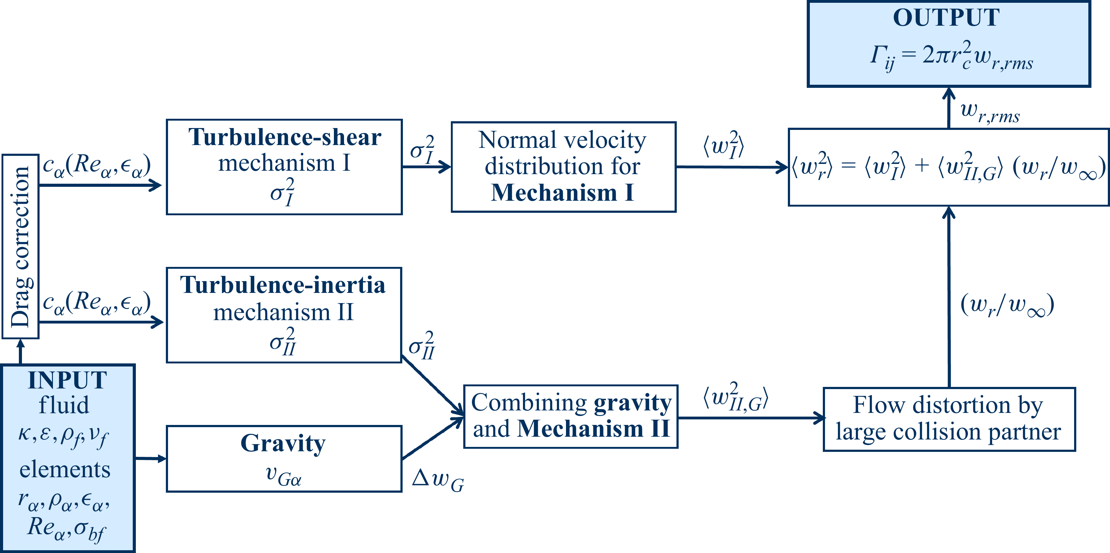
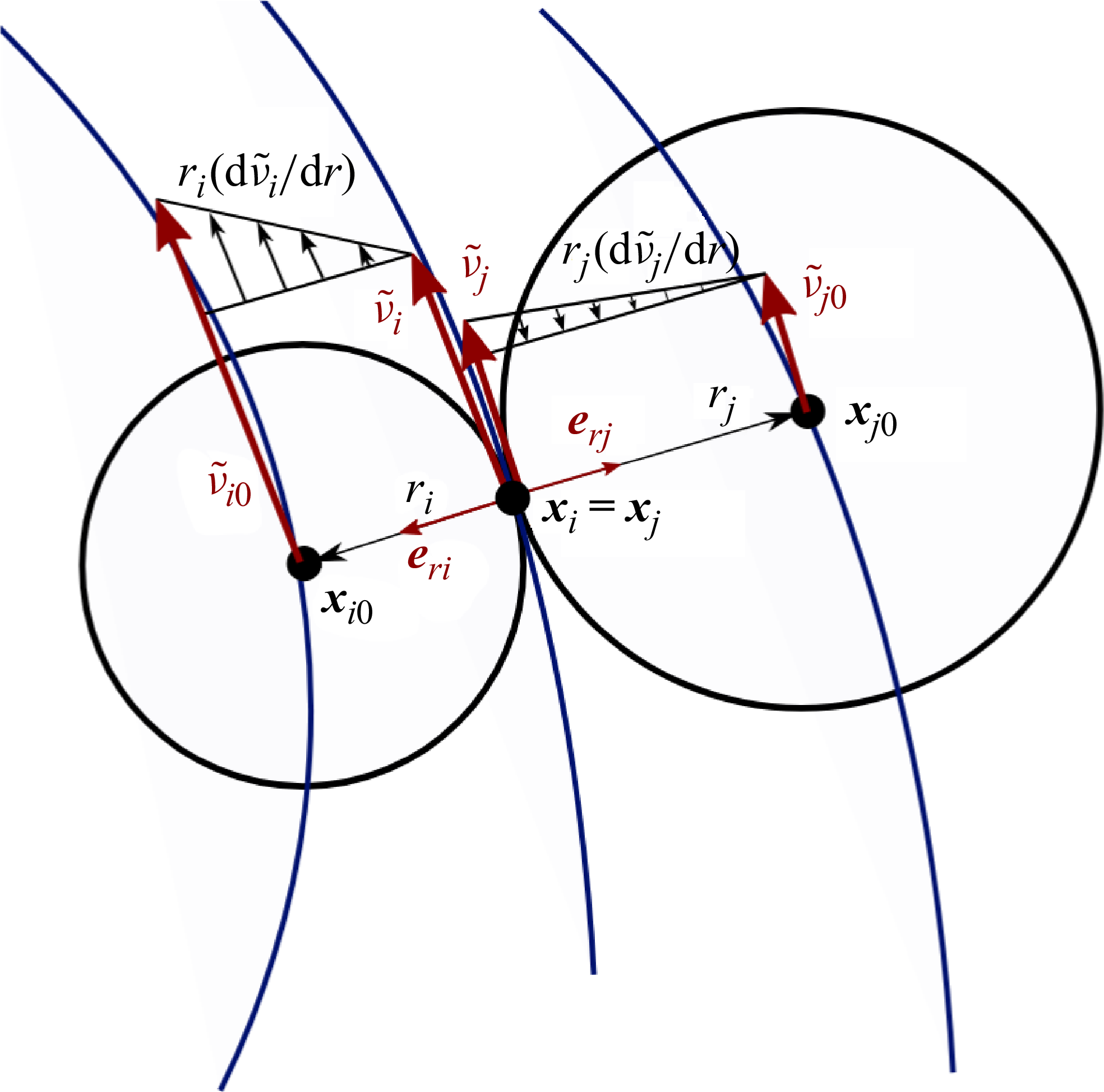
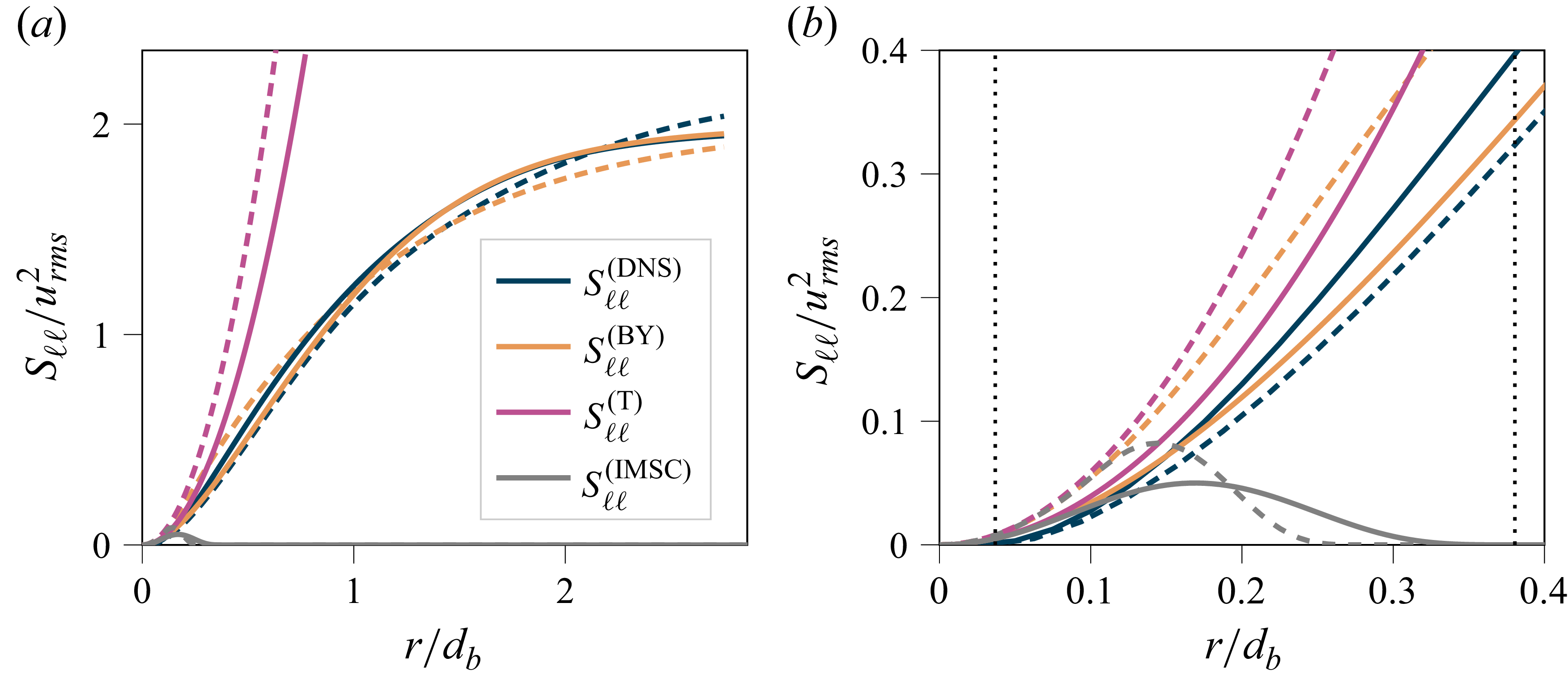


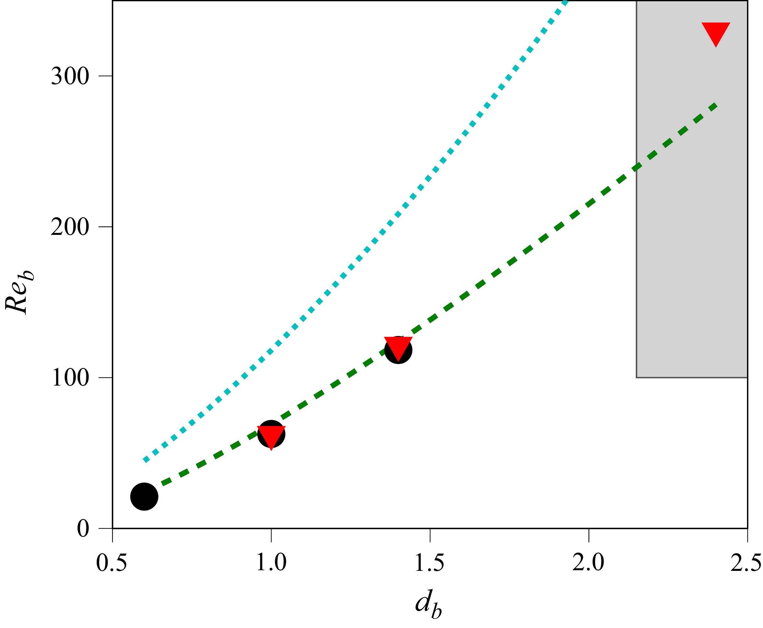


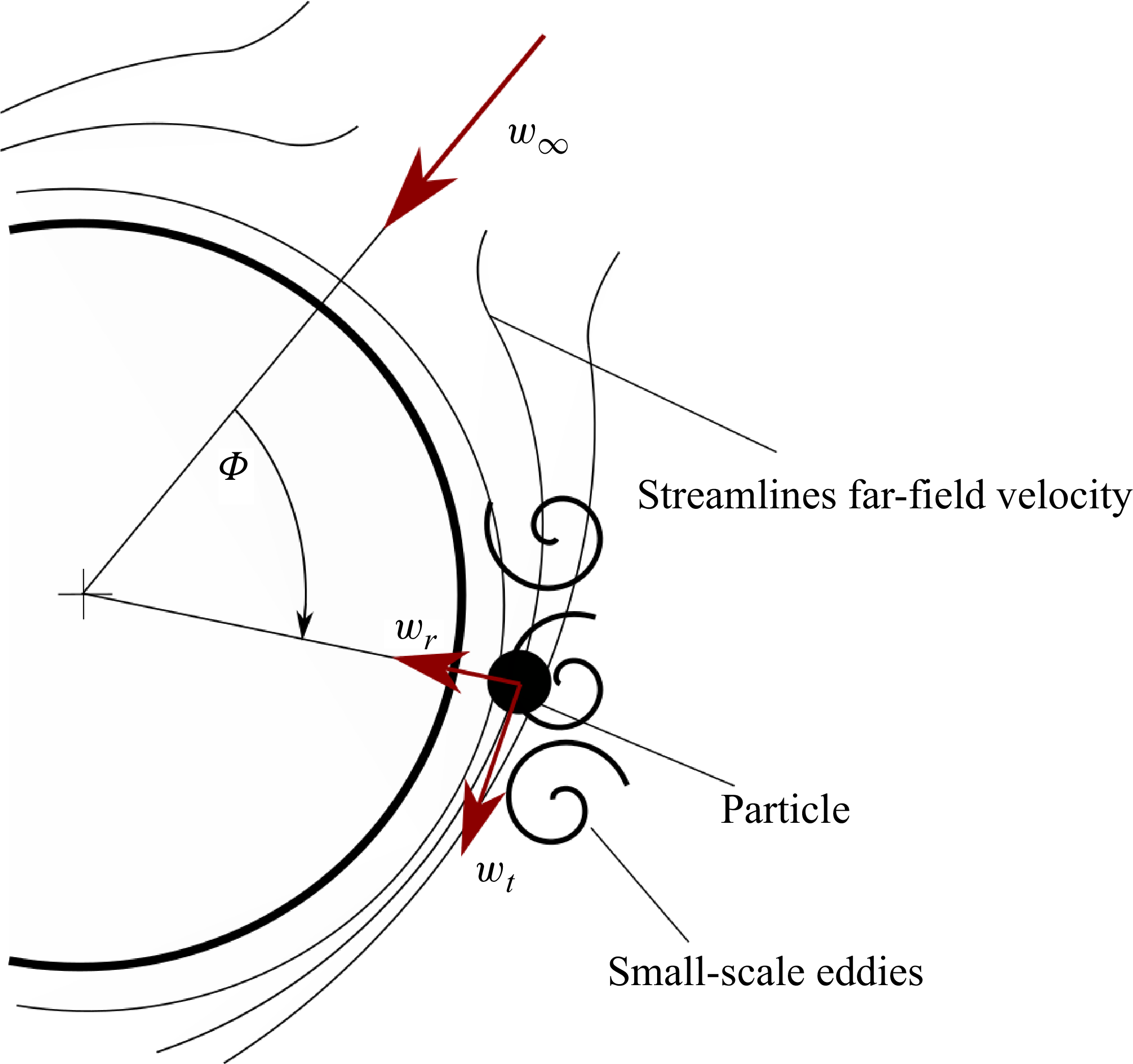
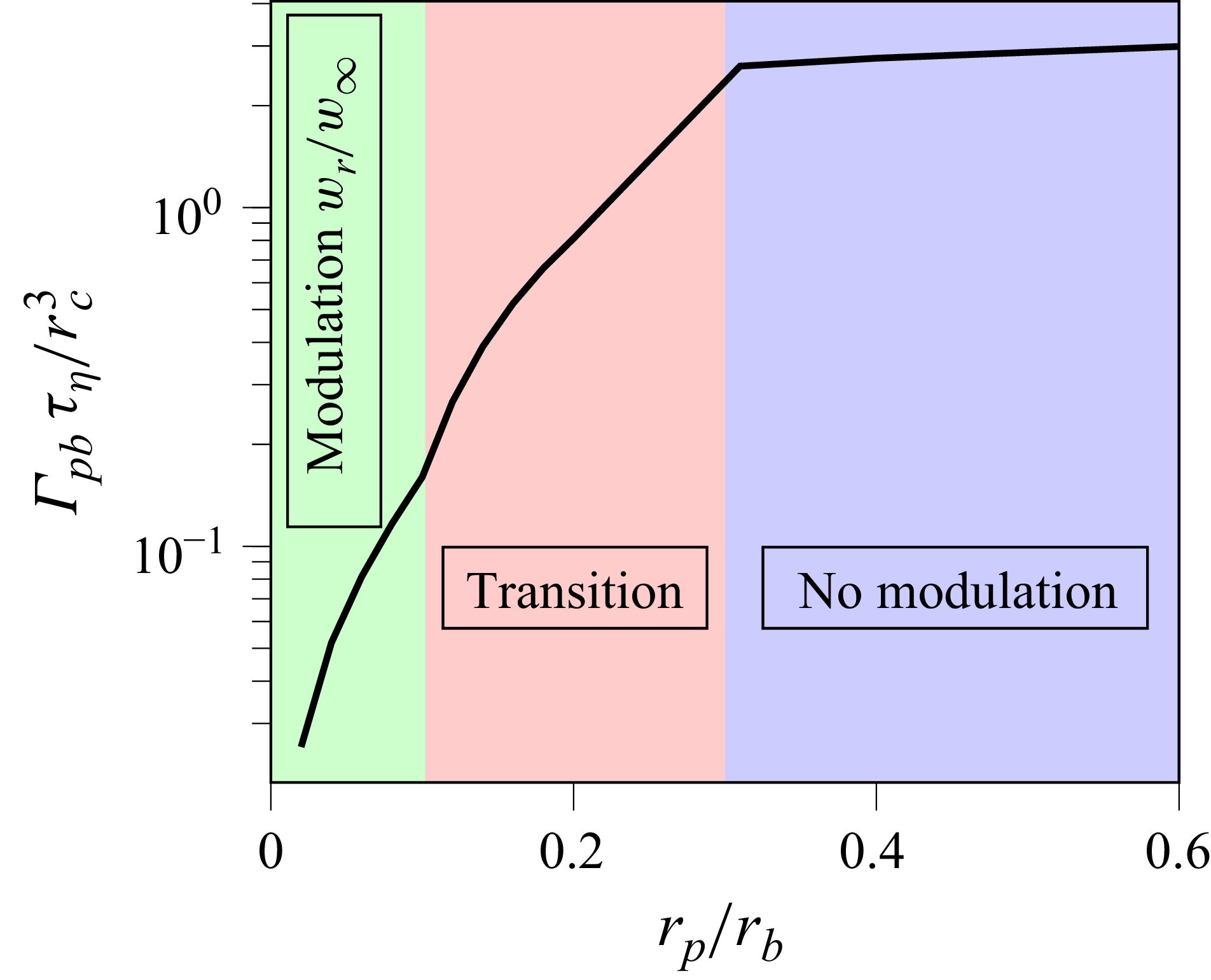


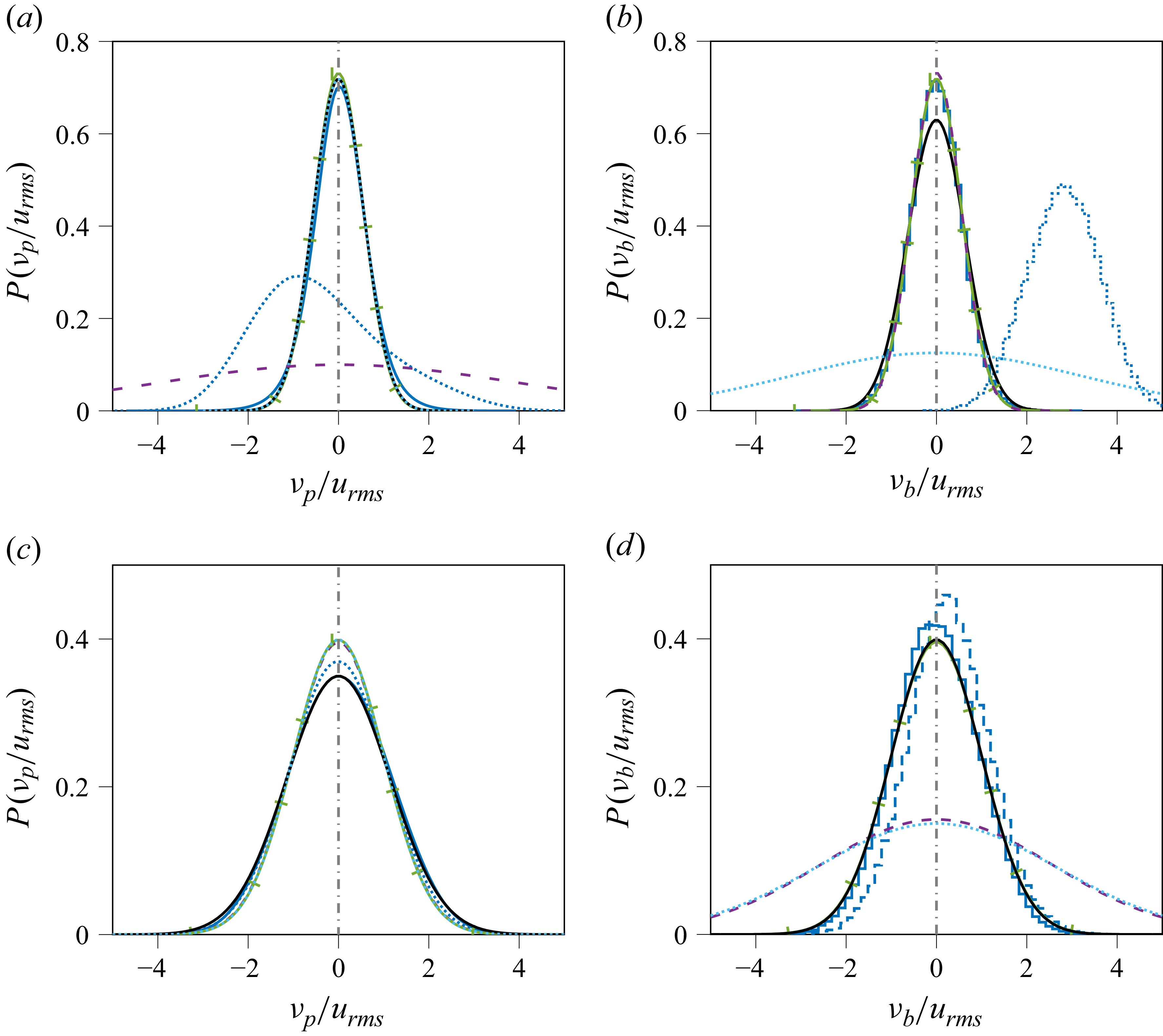


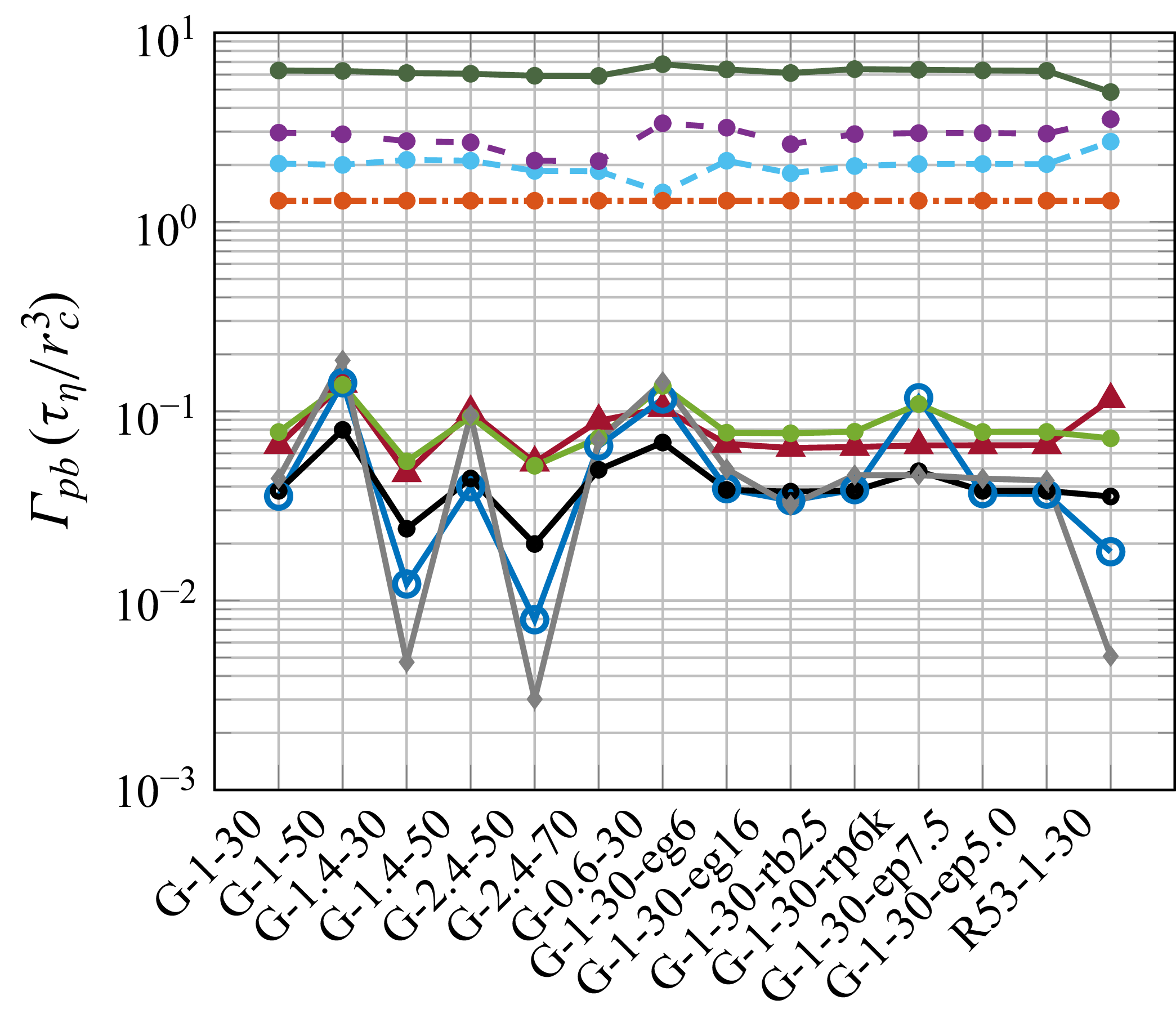
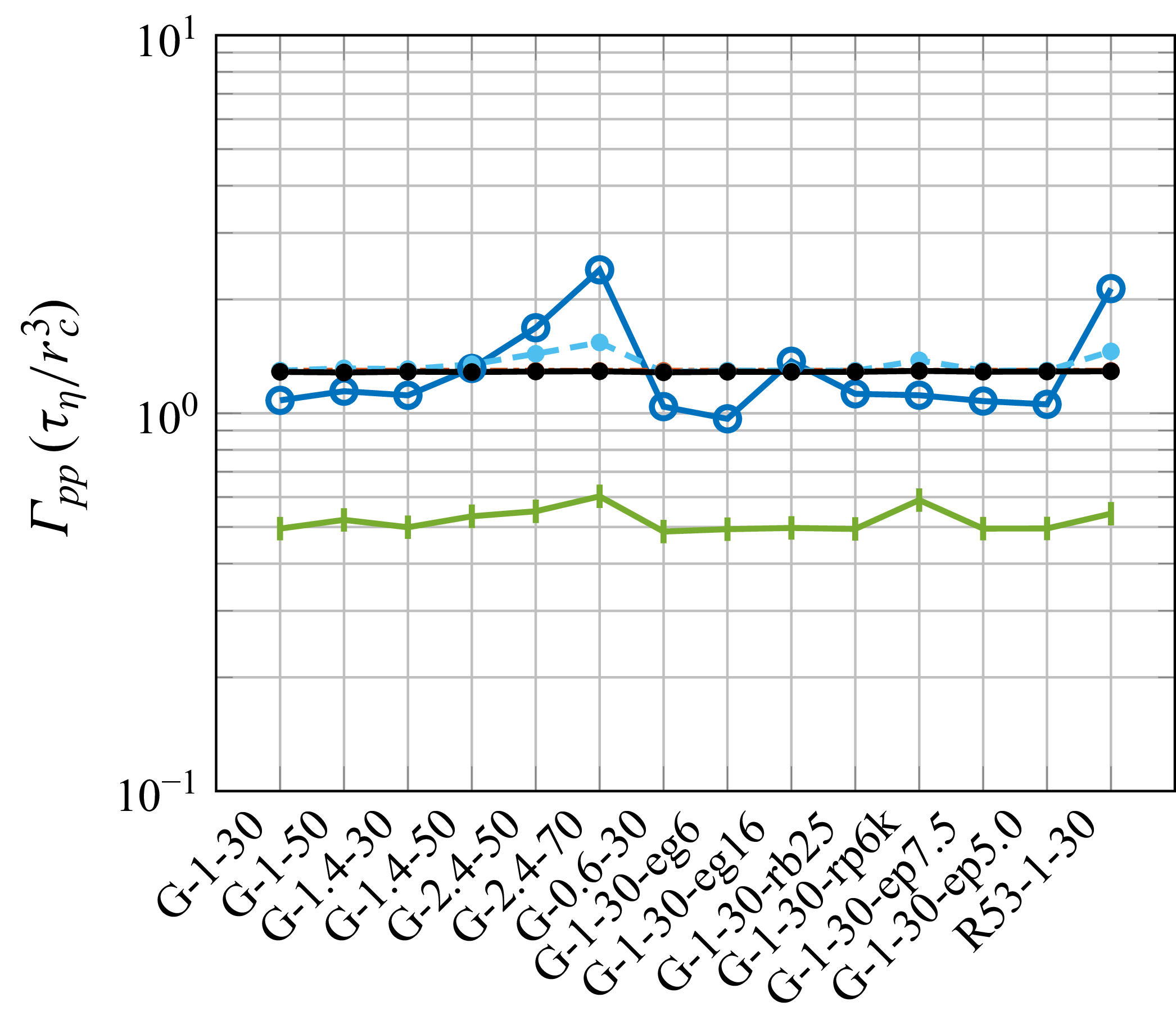
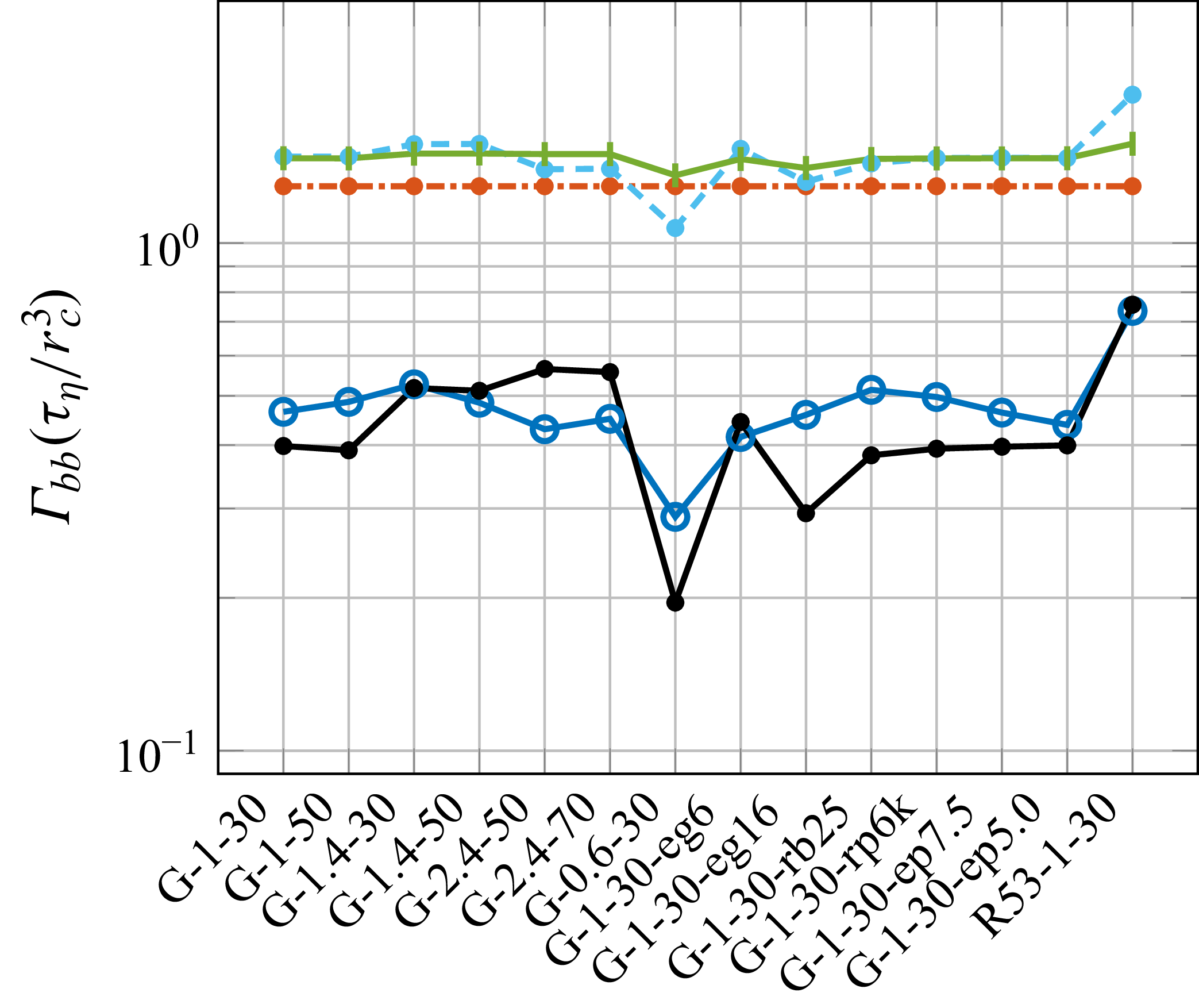
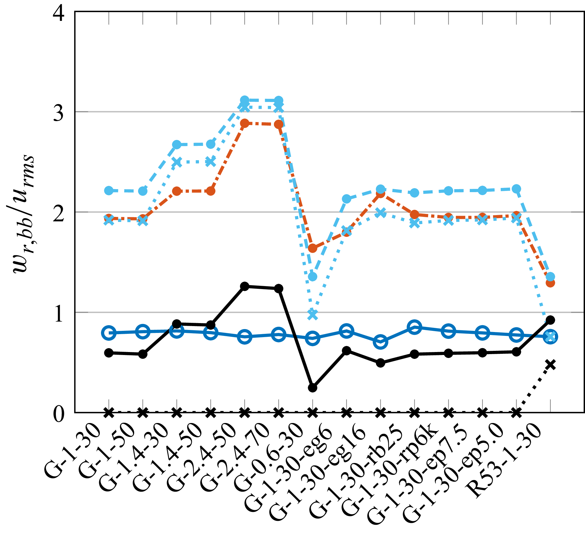

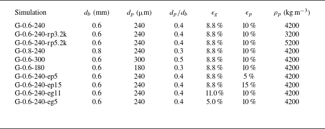
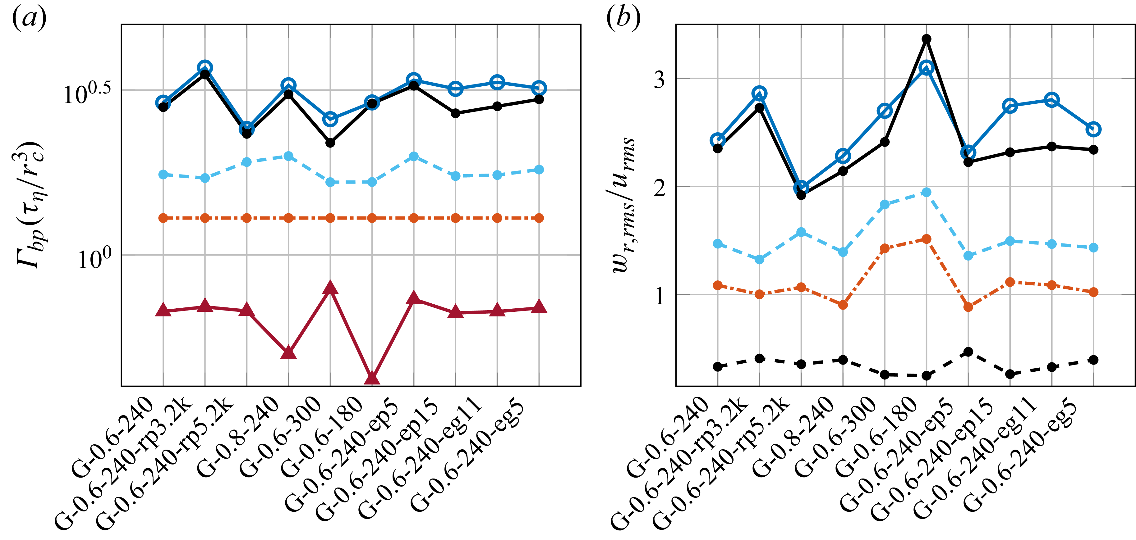
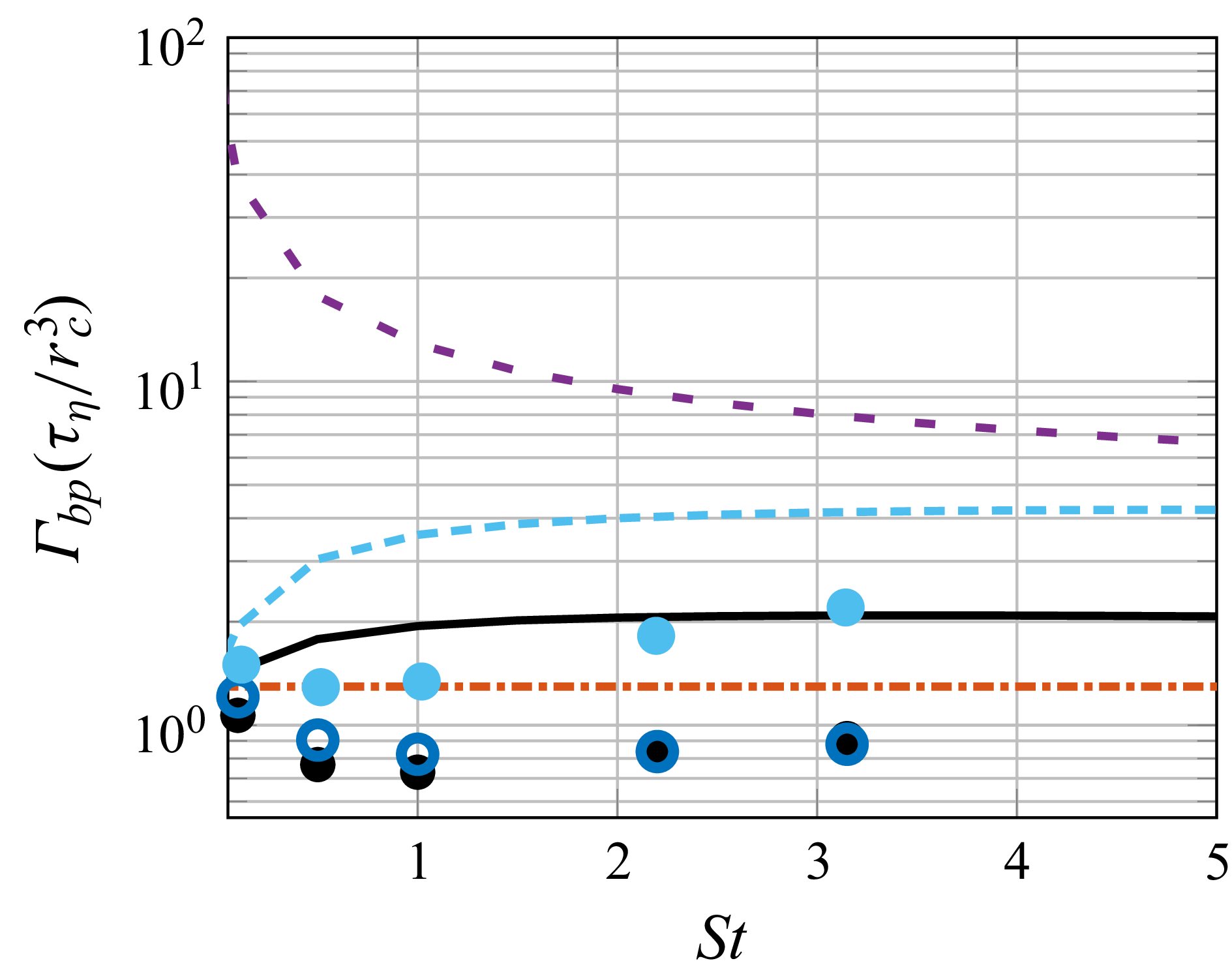


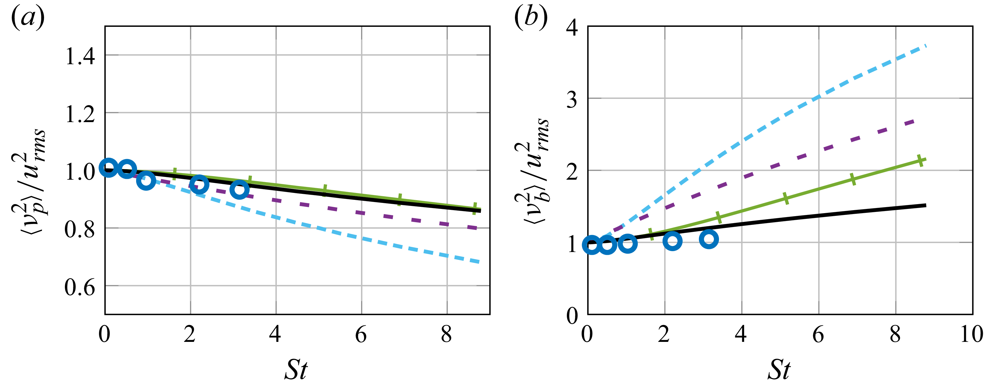

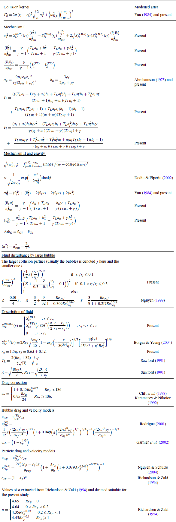
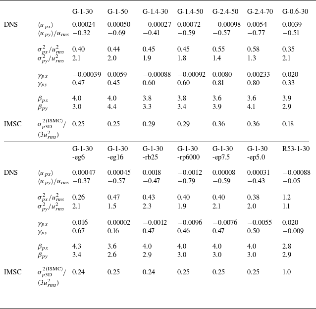


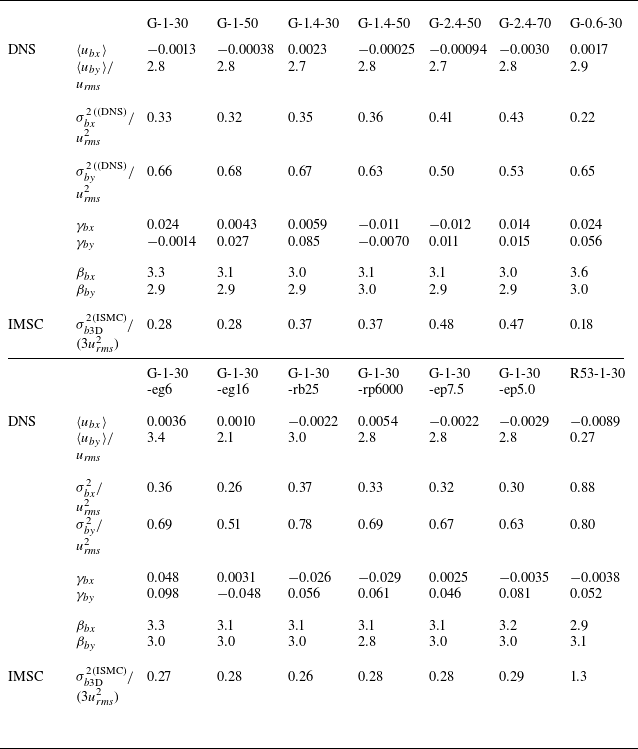


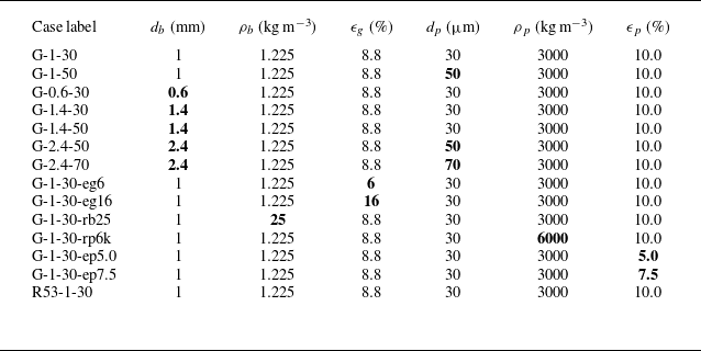

 Open access