


1. Introduction
In this paper we study semi-discrete unbalanced optimal transport problems: What is the optimal way of transporting a diffuse measure to a discrete measure (hence the name semi-discrete), where the two measures may have different total mass (hence the name unbalanced)? As an application, we study the unbalanced quantization problem: What is the best approximation of a diffuse measure by a discrete measure with respect to an unbalanced transport metric?
1.1. Unbalanced optimal transport
Classical optimal transport theory asks for the most efficient way to rearrange mass between two given probability distributions. Its origin goes back to 1781 and the French engineer Gaspard Monge, who was interested in the question of how to transport and reshape a pile of earth to form an embankment at minimal effort. It took over 200 years to develop a complete mathematical understanding of this problem, even to answer the question of whether there exists an optimal way of redistributing mass. Since the mathematical breakthroughs of the 1980s and 1990s, the field of optimal transport theory has thrived and found applications in crowd and traffic dynamics, economics, geometry, image and signal processing, machine learning and data science, PDEs and statistics. Depending on the context, mass may represent the distribution of particles (people or cars), supply and demand, population densities, etc. For thorough introductions see, e.g., [Reference Galichon27, Reference Peyré and Cuturi58, Reference Santambrogio61, Reference Villani69].
In classical optimal transport theory the initial and target measures must have the same total mass. In applications this is not always natural. Changes in mass may occur due to creation or annihilation of particles or a mismatch between supply and demand. Therefore so-called unbalanced transport problems, accounting for such differences, have recently received increased attention [Reference Chizat, Peyré, Schmitzer and Vialard18, Reference Figalli25, Reference Kondratyev, Monsaingeon and Vorotnikov39, Reference Liero, Mielke and Savaré45]. Brief overviews and discussions of various formulations can be found, for instance, in [Reference Chizat, Peyré, Schmitzer and Vialard19, Reference Schmitzer and Wirth64]. Further theoretical properties are examined in [Reference Laschos and Mielke41, Reference Liero, Mielke and Savaré46], examples for applications in data analysis can be found in [Reference Cai, Cheng, Schmitzer and Thorpe17, Reference Lavenant, Zhang, Kim and Schiebinger42, Reference Thual, Tran, Zemskova, Koyejo, Mohamed, Agarwal, Belgrave, Cho and Oh66]. In this article, we study the class of unbalanced transport problems called optimal entropy-transport problems from [Reference Liero, Mielke and Savaré45]; see Definition2.4. In particular, we develop this theory for the special case of semi-discrete transport.
1.2. Semi-discrete transport
Semi-discrete optimal transport theory is about the best way to transport a diffuse measure, $\mu \in L^1(\Omega)$
,
$\mu \in L^1(\Omega)$
, $\Omega \subset {\mathbb{R}}^d$
, to a discrete measure,
$\Omega \subset {\mathbb{R}}^d$
, to a discrete measure, $\nu = \sum _{i=1}^M m_i \delta _{x_i}$
. These type of problems arise naturally, for instance, in economics in computing the distance between a population with density
$\nu = \sum _{i=1}^M m_i \delta _{x_i}$
. These type of problems arise naturally, for instance, in economics in computing the distance between a population with density $\mu$
and a resource with distribution
$\mu$
and a resource with distribution $\nu = \sum _{i=1}^M m_i \delta _{x_i}$
, where
$\nu = \sum _{i=1}^M m_i \delta _{x_i}$
, where $x_i \in \Omega$
represent the locations of the resource and
$x_i \in \Omega$
represent the locations of the resource and $m_i \gt 0$
represent the size or capacity of the resource. The classical semi-discrete optimal transport problem, where
$m_i \gt 0$
represent the size or capacity of the resource. The classical semi-discrete optimal transport problem, where $\mu$
and
$\mu$
and $\nu$
are probability measures, has a nice geometric characterization. For example, for
$\nu$
are probability measures, has a nice geometric characterization. For example, for $p \in [1,\infty)$
, the Wasserstein-
$p \in [1,\infty)$
, the Wasserstein- $p$
metric
$p$
metric $W_p$
is defined by
$W_p$
is defined by
 \begin{equation*} W_p(\mu ,\nu) = \min \left \{ \sum _{i=1}^M \int _{T^{-1}(x_i)} |x-x_i|^p \mu (x) \, {\textrm {d}} x \, \right . \left | \, T\;:\;\Omega \to \{ x_i \}_{i=1}^M, \, \int _{T^{-1}(x_i)} \mu (x) \, {\textrm {d}} x = m_i \right \}^{1/p} \end{equation*}
where $\sum _{i=1}^M m_i = \int _{\Omega } \mu (x) \, {\textrm {d}} x = 1$
. This is an optimal partitioning (or assignment) problem, where the domain
$\sum _{i=1}^M m_i = \int _{\Omega } \mu (x) \, {\textrm {d}} x = 1$
. This is an optimal partitioning (or assignment) problem, where the domain $\Omega$
is partitioned into the regions
$\Omega$
is partitioned into the regions $T^{-1}(x_i)$
of mass
$T^{-1}(x_i)$
of mass $m_i$
,
$m_i$
, $i \in \{1,\ldots ,M\}$
, and each point
$i \in \{1,\ldots ,M\}$
, and each point $x \in T^{-1}(x_i)$
is assigned to point
$x \in T^{-1}(x_i)$
is assigned to point $x_i$
. For example, in two dimensions,
$x_i$
. For example, in two dimensions, $\Omega$
could represent a city,
$\Omega$
could represent a city, $\mu$
the population density of children,
$\mu$
the population density of children, $x_i$
and
$x_i$
and $m_i$
the location and size of schools,
$m_i$
the location and size of schools, $T^{-1}(x_i)$
the catchment areas of the schools, and
$T^{-1}(x_i)$
the catchment areas of the schools, and $W_p(\mu ,\nu)$
the cost of transporting the children to their assigned schools. If
$W_p(\mu ,\nu)$
the cost of transporting the children to their assigned schools. If $p=2$
, it turns out that the optimal partition
$p=2$
, it turns out that the optimal partition $\{T^{-1}(x_i)\}_{i=1}^M$
is a Laguerre diagram or power diagram, which is a type of weighted Voronoi diagram: There exist weights
$\{T^{-1}(x_i)\}_{i=1}^M$
is a Laguerre diagram or power diagram, which is a type of weighted Voronoi diagram: There exist weights $w_1,\ldots ,w_M \in {\mathbb{R}}$
such that
$w_1,\ldots ,w_M \in {\mathbb{R}}$
such that
 \begin{equation*} \overline {T^{-1}(x_i)} = \{ x \in \Omega \,|\, |x-x_i|^2 - w_i \leq |x-x_j|^2 - w_j \, \forall \, j \in \{1,\ldots ,M\} \}. \end{equation*}
The transport cells $T^{-1}(x_i)$
are the intersection of convex polytopes (polygons if
$T^{-1}(x_i)$
are the intersection of convex polytopes (polygons if $d=2$
, polyhedra if
$d=2$
, polyhedra if $d=3$
) with
$d=3$
) with $\Omega$
. The weights
$\Omega$
. The weights $w_1,\ldots ,w_M \in {\mathbb{R}}$
can be found by solving an unconstrained concave maximization problem. If
$w_1,\ldots ,w_M \in {\mathbb{R}}$
can be found by solving an unconstrained concave maximization problem. If $p=1$
, the optimal partition
$p=1$
, the optimal partition $\{T^{-1}(x_i)\}_{i=1}^M$
in an Apollonius diagram. See, e.g., [Reference Aurenhammer, Klein and Lee3, Sec. 6.4], [Reference Galichon27, Chap. 5], [Reference Kitagawa, Mérigot and Thibert37, Reference Mérigot, Thibert, Bonito and Nochetto52], [Reference Peyré and Cuturi58, Chap. 5], and Section 2.3 below, where we summarize the main results from classical semi-discrete optimal transport theory. Applications of semi-discrete transport include fluid mechanics [Reference Gallouët and Mérigot28, Reference Gallouët, Mérigot and Natale29], microstructure modelling [Reference Bourne, Kok, Roper and Spanjer10, Reference Buze, Feydy, Roper, Sedighiani and Bourne15], optics [Reference Meyron, Mérigot and Thibert53] and the Lagrangian discretization of Wasserstein gradient flows [Reference Leclerc, Mérigot, Santambrogio and Stra43] and mean field games [Reference Sarrazin63].
$\{T^{-1}(x_i)\}_{i=1}^M$
in an Apollonius diagram. See, e.g., [Reference Aurenhammer, Klein and Lee3, Sec. 6.4], [Reference Galichon27, Chap. 5], [Reference Kitagawa, Mérigot and Thibert37, Reference Mérigot, Thibert, Bonito and Nochetto52], [Reference Peyré and Cuturi58, Chap. 5], and Section 2.3 below, where we summarize the main results from classical semi-discrete optimal transport theory. Applications of semi-discrete transport include fluid mechanics [Reference Gallouët and Mérigot28, Reference Gallouët, Mérigot and Natale29], microstructure modelling [Reference Bourne, Kok, Roper and Spanjer10, Reference Buze, Feydy, Roper, Sedighiani and Bourne15], optics [Reference Meyron, Mérigot and Thibert53] and the Lagrangian discretization of Wasserstein gradient flows [Reference Leclerc, Mérigot, Santambrogio and Stra43] and mean field games [Reference Sarrazin63].
In Section 3, we extend these results to unbalanced transport, where $\mu$
and
$\mu$
and $\nu$
no longer need to have the same total mass, and the Wasserstein-
$\nu$
no longer need to have the same total mass, and the Wasserstein- $p$
metric is replaced by the unbalanced transport metric
$p$
metric is replaced by the unbalanced transport metric $W$
from Definition2.4. We prove that, also in the unbalanced case, the optimal partition is a type of generalized Laguerre diagram, and it can be found by solving a concave maximization problem for a set of weights
$W$
from Definition2.4. We prove that, also in the unbalanced case, the optimal partition is a type of generalized Laguerre diagram, and it can be found by solving a concave maximization problem for a set of weights $w_1,\ldots ,w_M$
; see Theorems3.1 and 3.3. This problem is natural from a modelling perspective, for example to describe a mismatch between the demand of a population
$w_1,\ldots ,w_M$
; see Theorems3.1 and 3.3. This problem is natural from a modelling perspective, for example to describe a mismatch between the demand of a population $\mu$
and the supply of a resource
$\mu$
and the supply of a resource $\nu$
and to model the prioritization of high-density regions at the expense of areas with a low population density.
$\nu$
and to model the prioritization of high-density regions at the expense of areas with a low population density.
For unbalanced transport, there is no one, definitive transport cost, but many models are conceivable. As a first application of our theory of semi-discrete unbalanced transport, in Examples3.14 and 3.15, we use it to compare different unbalanced transport models. As a second application, in Section 4, we apply it to the quantization problem.
1.3. Quantization
Quantization of measures refers to the problem of finding the best approximation of a diffuse measure by a discrete measure [Reference Graf and Luschgy32], [Reference Gruber35, Sec. 33]. For example, the classical quantization problem with respect to the Wasserstein- $p$
metric,
$p$
metric, $p \in [1,\infty)$
, is the following: Given
$p \in [1,\infty)$
, is the following: Given $\mu \in L^1(\Omega)$
,
$\mu \in L^1(\Omega)$
, $\Omega \subset {\mathbb{R}}^d$
,
$\Omega \subset {\mathbb{R}}^d$
, $\int _\Omega \mu (x) \, {\textrm {d}} x = 1$
, find a discrete probability measure
$\int _\Omega \mu (x) \, {\textrm {d}} x = 1$
, find a discrete probability measure $\nu = \sum _{i=1}^M m_i \delta _{x_i}$
that gives the best approximation of
$\nu = \sum _{i=1}^M m_i \delta _{x_i}$
that gives the best approximation of $\mu$
in the Wasserstein-
$\mu$
in the Wasserstein- $p$
metric,
$p$
metric,
 \begin{equation} Q^M_p(\mu) = \min \left \{ W_p^p(\mu ,\nu) \, \Bigg | \, \nu = \sum _{i=1}^M m_i \delta _{x_i}, \; x_1,\ldots ,x_M \in \Omega , \; m_i \gt 0, \; \sum _{i=1}^M m_i=1 \right \}. \end{equation}
We call $Q^M_p$
the quantization error. Problems of this form arise in a wide range of applications including economic planning and optimal location problems [Reference Bollobás and Stern7, Reference Bouchitté, Jimenez and Mahadevan8, Reference Buttazzo and Santambrogio14], finance [Reference Pagès, Pham, Printems and Rachev57], numerical integration [Reference Du, Faber and Gunzburger21, Sec. 2.2], [Reference Pagès, Pham, Printems and Rachev57, Sec. 2.3], energy-driven pattern formation [Reference Bourne, Peletier and Roper11, Reference Larsson, Choksi and Nave40] and approximation of initial data for particle (meshfree) methods for PDEs. An approach to quantization using gradient flows is given in [Reference Caglioti, Golse and Iacobelli16, Reference Iacobelli, Cardaliaguet, Porretta and Salvarani36]. We mention a few important variations on the classical quantization problem. The case where the masses
$Q^M_p$
the quantization error. Problems of this form arise in a wide range of applications including economic planning and optimal location problems [Reference Bollobás and Stern7, Reference Bouchitté, Jimenez and Mahadevan8, Reference Buttazzo and Santambrogio14], finance [Reference Pagès, Pham, Printems and Rachev57], numerical integration [Reference Du, Faber and Gunzburger21, Sec. 2.2], [Reference Pagès, Pham, Printems and Rachev57, Sec. 2.3], energy-driven pattern formation [Reference Bourne, Peletier and Roper11, Reference Larsson, Choksi and Nave40] and approximation of initial data for particle (meshfree) methods for PDEs. An approach to quantization using gradient flows is given in [Reference Caglioti, Golse and Iacobelli16, Reference Iacobelli, Cardaliaguet, Porretta and Salvarani36]. We mention a few important variations on the classical quantization problem. The case where the masses $m_1,\ldots ,m_M$
are fixed and the minimization in (1.1) is only taken over
$m_1,\ldots ,m_M$
are fixed and the minimization in (1.1) is only taken over $x_1,\ldots ,x_M$
is considered for example in [Reference Bourne, Kok, Roper and Spanjer10, Reference Mérigot, Santambrogio, Sarrazin, Ranzato, Beygelzimer, Dauphin, Liang and Wortman Vaughan51, Reference Xin, Lévy and Chen70]. The case where
$x_1,\ldots ,x_M$
is considered for example in [Reference Bourne, Kok, Roper and Spanjer10, Reference Mérigot, Santambrogio, Sarrazin, Ranzato, Beygelzimer, Dauphin, Liang and Wortman Vaughan51, Reference Xin, Lévy and Chen70]. The case where $\mu$
is a discrete measure, with support of cardinality
$\mu$
is a discrete measure, with support of cardinality $N \gg M$
, has applications in image and signal compression [Reference Du, Gunzburger, Ju and Wang22, Reference Gersho and Gray31] and data clustering (
$N \gg M$
, has applications in image and signal compression [Reference Du, Gunzburger, Ju and Wang22, Reference Gersho and Gray31] and data clustering ( $k$
-means clustering) [Reference MacQueen49, Reference Thorpe, Theil, Johansen and Cade65]. If
$k$
-means clustering) [Reference MacQueen49, Reference Thorpe, Theil, Johansen and Cade65]. If $\nu$
is a one-dimensional measure (supported on a set of Hausdorff dimension
$\nu$
is a one-dimensional measure (supported on a set of Hausdorff dimension $1$
), then the quantization problem is known as the irrigation problem [Reference Lu and Slepčev48, Reference Mosconi and Tilli55]. In this paper, we consider the variation where the Wasserstein-
$1$
), then the quantization problem is known as the irrigation problem [Reference Lu and Slepčev48, Reference Mosconi and Tilli55]. In this paper, we consider the variation where the Wasserstein- $p$
metric in (1.1) is replaced by an unbalanced transport metric.
$p$
metric in (1.1) is replaced by an unbalanced transport metric.
It can be shown that the quantization problem (1.1) can be rewritten as an optimization problem in terms of the particle locations $\{ x_i \}_{i=1}^M$
and their Voronoi tessellation:
$\{ x_i \}_{i=1}^M$
and their Voronoi tessellation:
 \begin{equation} Q^M_p(\mu) = \min \left \{ J(x_1,\ldots ,x_M) \, | \, x_1,\ldots ,x_M \in \Omega \right \} \end{equation}
where
 \begin{equation*} J(x_1,\ldots ,x_M) = \sum _{i=1}^M \int _{V_i(x_1,\ldots ,x_M)} |x-x_i|^p \mu (x) \, {\textrm {d}} x \end{equation*}
and where $\{ V_i \}_{i=1}^M$
is the Voronoi diagram generated by
$\{ V_i \}_{i=1}^M$
is the Voronoi diagram generated by $\{x_i\}_{i=1}^M$
,
$\{x_i\}_{i=1}^M$
,
 \begin{equation*} V_i = V_i(x_1,\ldots ,x_M) = \left \{ x \in \Omega \,\big |\, |x-x_i| \leq |x-x_j| \textrm { for all } j\in \{1,\ldots ,M\} \right \}. \end{equation*}
If $(x_1, \ldots , x_M)$
is a global minimizer of
$(x_1, \ldots , x_M)$
is a global minimizer of $J$
, then
$J$
, then $\sum _{i=1}^M \left (\int _{V_i} \mu \, {\textrm {d}} x \right) \delta _{x_i}$
is an optimal quantizer of
$\sum _{i=1}^M \left (\int _{V_i} \mu \, {\textrm {d}} x \right) \delta _{x_i}$
is an optimal quantizer of $\mu$
with respect to the Wasserstein-
$\mu$
with respect to the Wasserstein- $p$
metric. See for instance [Reference Bourne, Peletier and Roper11, Sec. 4.1], [Reference Kloeckner38, Sec. 7] and Theorem4.2. In the vector quantization (electrical engineering), literature
$p$
metric. See for instance [Reference Bourne, Peletier and Roper11, Sec. 4.1], [Reference Kloeckner38, Sec. 7] and Theorem4.2. In the vector quantization (electrical engineering), literature $J$
is known as the distortion of the quantizer [Reference Gersho and Gray31].
$J$
is known as the distortion of the quantizer [Reference Gersho and Gray31].
The quantization problem with respect to the Wasserstein-2 metric is particularly well studied. In this case, it can be shown that critical points of $J$
are generators of centroidal Voronoi tessellations (CVTs) of
$J$
are generators of centroidal Voronoi tessellations (CVTs) of $M$
points [Reference Du, Faber and Gunzburger21]; this means that
$M$
points [Reference Du, Faber and Gunzburger21]; this means that $\nabla J(x_1,\ldots ,x_M)=0$
if and only if
$\nabla J(x_1,\ldots ,x_M)=0$
if and only if $x_i$
is the centre of mass of its own Voronoi cell
$x_i$
is the centre of mass of its own Voronoi cell $V_i$
for all
$V_i$
for all $i$
,
$i$
,
 \begin{equation} x_i = \frac {\displaystyle \int _{V_i(x_1,\ldots ,x_M)} x \mu (x) \, {\textrm {d}} x}{ \int _{V_i(x_1,\ldots ,x_M)} \mu (x) \, {\textrm {d}} x}, \quad i \in \{1,\ldots ,M\}. \end{equation}
In general, there does not exist a unique CVT of $M$
points, as illustrated in Figure 1, and
$M$
points, as illustrated in Figure 1, and $J$
is non-convex with many local minimizers for large
$J$
is non-convex with many local minimizers for large $M$
. Equation (1.3) is a nonlinear system of equations for
$M$
. Equation (1.3) is a nonlinear system of equations for $x_1,\ldots ,x_M$
. A simple and popular method for computing CVTs is Lloyd’s algorithm [Reference Du, Faber and Gunzburger21, Reference Emelianenko, Ju and Rand24, Reference Lloyd47, Reference Sabin and Gray60], which is a fixed point method for solving the Euler–Lagrange equations (1.3).
$x_1,\ldots ,x_M$
. A simple and popular method for computing CVTs is Lloyd’s algorithm [Reference Du, Faber and Gunzburger21, Reference Emelianenko, Ju and Rand24, Reference Lloyd47, Reference Sabin and Gray60], which is a fixed point method for solving the Euler–Lagrange equations (1.3).
Two (approximate) centroidal Voronoi tessellations (CVTs) of 10 points for the uniform density $\mu =1$
on a unit square. The polygons are the centroidal Voronoi cells
$\mu =1$
on a unit square. The polygons are the centroidal Voronoi cells $V_i$
and the circles are the generators
$V_i$
and the circles are the generators $x_i$
. The CVTs were computed using Lloyd’s algorithm. The CVT on the left has a lower energy
$x_i$
. The CVTs were computed using Lloyd’s algorithm. The CVT on the left has a lower energy $J$
than the CVT on the right. The corresponding quantizer
$J$
than the CVT on the right. The corresponding quantizer $\nu =\sum _{i=1}^{10} m_i \delta _{x_i}$
of
$\nu =\sum _{i=1}^{10} m_i \delta _{x_i}$
of $\mu$
is reconstructed from the CVT by taking
$\mu$
is reconstructed from the CVT by taking $m_i$
as the areas of the centroidal Voronoi cells and
$m_i$
as the areas of the centroidal Voronoi cells and $x_i$
as their generators.
$x_i$
as their generators.

In Sections 4.1 and 4.2 we extend these results to unbalanced quantization, where the Wasserstein- $p$
metric in (1.1) is replaced by the unbalanced transport metric
$p$
metric in (1.1) is replaced by the unbalanced transport metric $W$
(defined in equation (2.6)), and where
$W$
(defined in equation (2.6)), and where $\mu$
and
$\mu$
and $\nu$
need not have the same total mass. In Theorem4.2 we prove an expression of the form (1.2), which states that the unbalanced quantization problem can be reduced to an optimization problem for the locations
$\nu$
need not have the same total mass. In Theorem4.2 we prove an expression of the form (1.2), which states that the unbalanced quantization problem can be reduced to an optimization problem for the locations $x_1,\ldots ,x_M$
of the Dirac masses. This optimization problem is again formulated in terms of the Voronoi diagram generated by
$x_1,\ldots ,x_M$
of the Dirac masses. This optimization problem is again formulated in terms of the Voronoi diagram generated by $x_1,\ldots ,x_M$
. In Section 4.2 we solve the unbalanced quantization problem numerically, which includes extending Lloyd’s algorithm to the unbalanced case.
$x_1,\ldots ,x_M$
. In Section 4.2 we solve the unbalanced quantization problem numerically, which includes extending Lloyd’s algorithm to the unbalanced case.
We conclude the paper in subsection 4.3 by studying the asymptotic unbalanced quantization problem: What is the optimal configuration of the particles $x_1,\ldots ,x_M$
as
$x_1,\ldots ,x_M$
as $M \to \infty$
and how does the quantization error scale in
$M \to \infty$
and how does the quantization error scale in $M$
? Consider for example the classical quantization problem (1.1) with
$M$
? Consider for example the classical quantization problem (1.1) with $p=2$
,
$p=2$
, $|\Omega |=1$
,
$|\Omega |=1$
, $\mu =1$
(i.e.,
$\mu =1$
(i.e., $\mu$
is the Lebesgue measure on
$\mu$
is the Lebesgue measure on $\Omega$
), and
$\Omega$
), and $M$
fixed. From above, we know that an optimal quantizer
$M$
fixed. From above, we know that an optimal quantizer $\nu$
corresponds to an optimal CVT of
$\nu$
corresponds to an optimal CVT of $M$
points, where optimal means that the CVT has lowest energy
$M$
points, where optimal means that the CVT has lowest energy $J$
amongst all CVTs of
$J$
amongst all CVTs of $M$
points. Gersho [Reference Gersho30] conjectured that, as
$M$
points. Gersho [Reference Gersho30] conjectured that, as $M \to \infty$
, the Voronoi cells of the optimal CVT asymptotically have the same shape, i.e., asymptotically they are translations and rescalings of a single polytope. In two dimensions (
$M \to \infty$
, the Voronoi cells of the optimal CVT asymptotically have the same shape, i.e., asymptotically they are translations and rescalings of a single polytope. In two dimensions ( $d=2$
), various versions of Gersho’s Conjecture have been proved independently by several authors [Reference Bollobás and Stern7, Reference Gruber33, Reference Morgan and Bolton54, Reference Newman56, Reference Tóth67, Reference Tóth68]. Roughly speaking, it has been shown that the hexagonal tiling is optimal as
$d=2$
), various versions of Gersho’s Conjecture have been proved independently by several authors [Reference Bollobás and Stern7, Reference Gruber33, Reference Morgan and Bolton54, Reference Newman56, Reference Tóth67, Reference Tóth68]. Roughly speaking, it has been shown that the hexagonal tiling is optimal as $M \to \infty$
. In other words, arranging the seeds
$M \to \infty$
. In other words, arranging the seeds $x_1,\ldots ,x_M$
in a regular triangular lattice is asymptotically optimal. This crystallization result can be stated more precisely as follows: If
$x_1,\ldots ,x_M$
in a regular triangular lattice is asymptotically optimal. This crystallization result can be stated more precisely as follows: If $\Omega$
is a convex polygon with at most 6 sides, then
$\Omega$
is a convex polygon with at most 6 sides, then
 \begin{equation} J(x_1,\ldots ,x_M) \ge \frac {5 \sqrt {3}}{54} \frac {1}{M} \end{equation}
where the right-hand side is the energy of a regular triangular lattice of $M$
points such that the Voronoi cells
$M$
points such that the Voronoi cells $V_i$
are regular hexagons of area
$V_i$
are regular hexagons of area $1/M$
. In general, this lower bound is not attained for finite
$1/M$
. In general, this lower bound is not attained for finite $M$
(unless
$M$
(unless $\Omega$
is a regular hexagon and
$\Omega$
is a regular hexagon and $M=1$
), but it is attained in limit
$M=1$
), but it is attained in limit $M \to \infty$
:
$M \to \infty$
:
 \begin{equation} \lim _{M \to \infty } M \cdot Q_2^M(1) = \lim _{M \to \infty } M \cdot \min _{x_i \in \Omega } J(x_1,\ldots ,x_M) = \frac {5 \sqrt {3}}{54}. \end{equation}
See the references above or [Reference Bourne, Peletier and Theil12, Thm. 5]. We generalize (1.4) and (1.5) to the unbalanced quantization problem in Theorem4.7 and Theorem4.12, respectively. Roughly speaking, we show that again for $\mu =1$
the triangular lattice is optimal in the limit
$\mu =1$
the triangular lattice is optimal in the limit $M \to \infty$
. For general
$M \to \infty$
. For general $\mu \in L^1(\Omega)$
, it is asymptotically optimal for the particles to locally form a triangular lattice with density determined by a nonlocal function of
$\mu \in L^1(\Omega)$
, it is asymptotically optimal for the particles to locally form a triangular lattice with density determined by a nonlocal function of $\mu$
.
$\mu$
.
While our quantization results are limited to two dimensions, this is also largely true for the classical quantization problem. In three dimensions, it is not known whether Gersho’s conjecture holds, although there is some numerical evidence for the case $p=2$
that optimal CVTs of
$p=2$
that optimal CVTs of $M$
points tend as
$M$
points tend as $M \to \infty$
to the Voronoi diagram of the body-centered cubic (BCC) lattice, where each Voronoi cell is congruent to a truncated octahedron [Reference Du and Wang23]. See also [Reference Choksi and Lu20]. For
$M \to \infty$
to the Voronoi diagram of the body-centered cubic (BCC) lattice, where each Voronoi cell is congruent to a truncated octahedron [Reference Du and Wang23]. See also [Reference Choksi and Lu20]. For $p=2$
, it has been proved that, amongst lattices, the BCC lattice is optimal [Reference Barnes and Sloane5].
$p=2$
, it has been proved that, amongst lattices, the BCC lattice is optimal [Reference Barnes and Sloane5].
For general $p$
,
$p$
, $d$
and
$d$
and $\mu$
, the scaling of the quantization error is known even if the optimal quantizer is not; Zador’s theorem [Reference Zador71], [Reference Gruber35, Cor. 33.3] states that
$\mu$
, the scaling of the quantization error is known even if the optimal quantizer is not; Zador’s theorem [Reference Zador71], [Reference Gruber35, Cor. 33.3] states that
 \begin{equation} \lim _{M \to \infty } M^{\frac pd} \cdot Q^M_p(\mu) = c(p,d) \, \| \mu \|_{L^{\frac {d}{d+p}}(\Omega)} \end{equation}
where the constant $c(p,d)$
is characterized by
$c(p,d)$
is characterized by
 \begin{equation*} c(p,d) = \lim _{M \to \infty } M^{\frac pd} \cdot Q^M_p(\mathcal{L} {{\LARGE \llcorner }}{[0,1]^d}), \end{equation*}
and where $\mathcal{L}$
is the
$\mathcal{L}$
is the $d$
-dimensional Lebesgue measure. For a modern proof using
$d$
-dimensional Lebesgue measure. For a modern proof using $\Gamma$
-convergence see [Reference Bouchitté, Jimenez and Rajesh9] and [Reference Santambrogio62, Proposition 7.21]. For generalizations to quantization on Riemannian manifolds see [Reference Gruber34], [Reference Kloeckner38, Thm. 1.2] and [Reference Aydın and Iacobelli4]. It is an open problem to compute the optimal constant
$\Gamma$
-convergence see [Reference Bouchitté, Jimenez and Rajesh9] and [Reference Santambrogio62, Proposition 7.21]. For generalizations to quantization on Riemannian manifolds see [Reference Gruber34], [Reference Kloeckner38, Thm. 1.2] and [Reference Aydın and Iacobelli4]. It is an open problem to compute the optimal constant $c(p,d)$
except for
$c(p,d)$
except for $d=1$
and
$d=1$
and $d=2$
, where
$d=2$
, where
 \begin{equation} c(p,1) = \int _{-1/2}^{1/2} |x|^p \, {\textrm {d}} x, \qquad c(p,2) = \int _{H(1)} |x|^p \, {\textrm {d}} x, \end{equation}
where $H(1)$
is a regular hexagon of area
$H(1)$
is a regular hexagon of area $1$
centred at the origin
$1$
centred at the origin $0$
. We recover Zador’s theorem for the case
$0$
. We recover Zador’s theorem for the case $d=2$
, along with the optimal constant
$d=2$
, along with the optimal constant $c(p,2)$
, as a special case of Theorem4.12; see Example4.18.
$c(p,2)$
, as a special case of Theorem4.12; see Example4.18.
1.4. Outline and contribution
Section 2 collects relevant results from classical, unbalanced and semi-discrete transport, which will be generalized in Section 3 to the case of semi-discrete unbalanced transport. Finally, Section 4 considers the unbalanced quantization problem.
In more detail, the contributions of this article are the following.
-
• Section 3.1: We extend semi-discrete transport theory to the unbalanced case, most importantly a simple, geometric tessellation formulation (Theorem3.1), optimality conditions that fully characterize primal and dual solutions (Theorem3.3) and additional different primal and dual convex formulations. Unlike in the balanced case, the dual potentials associated with the discrete mass locations do not only determine the tessellation of the continuous measure but also the density of the optimal transport plan. Particular attention needs to be paid to areas where the ground transport cost function becomes infinite. Special cases of these results were derived in [Reference Leclerc, Mérigot, Santambrogio and Stra43, Reference Sarrazin63] to study a Lagrangian discretization of Wasserstein gradient flows and variational mean field games.
-
• Section 3.2: We develop numerical algorithms for solving the semi-discrete unbalanced transport problem and numerically illustrate novel phenomena of unbalanced transport (Example3.14). In particular, we show qualitative differences between different unbalanced transport models and examine the effect of changing the length scale, which typically is intrinsic to unbalanced transport models.
-
• Sections 4.1 and 4.2: We extend the theory of optimal transport-based quantization of measures to unbalanced transport, deriving in particular an equivalent Voronoi tessellation problem (Theorem4.2), which turns out to be a natural generalization of the known corresponding formulation in classical transport. The interesting fact here is that the simple geometric Voronoi tessellation structure survives when passing from balanced to unbalanced transport, but the mass of the generating points now depends in a more complex way on the mass within their cells. We also illustrate unbalanced quantization numerically, extending the standard algorithms (including Lloyd’s algorithm) to the unbalanced case.
-
• Section 4.3: In two spatial dimensions, where crystallization results from discrete geometry are available, we derive the optimal asymptotic quantization cost and the optimal asymptotic point density for quantizing a given measure $\mu$
using unbalanced transport (Theorem4.12). Our result includes Zador’s theorem for classical, balanced quantization as a special case; see Example4.18. As is common in asymptotic quantization, we consider a spatial rescaling of the domain as the number of points increases and the most interesting regime is where the rescaled point density converges to a non-zero, finite limit. While in the balanced case the rescaled asymptotic cost only depends on the growth behaviour of the transport ground cost function, in the unbalanced setting we now observe an interplay between the rescaled point density and the intrinsic length scale of unbalanced transport. An interesting, novel effect in this unbalanced setting is that the optimal point density depends nonlocally on the global mass distribution in such a way that whole regions with positive measure may be completely neglected in favour of regions with higher mass.
$\mu$
using unbalanced transport (Theorem4.12). Our result includes Zador’s theorem for classical, balanced quantization as a special case; see Example4.18. As is common in asymptotic quantization, we consider a spatial rescaling of the domain as the number of points increases and the most interesting regime is where the rescaled point density converges to a non-zero, finite limit. While in the balanced case the rescaled asymptotic cost only depends on the growth behaviour of the transport ground cost function, in the unbalanced setting we now observe an interplay between the rescaled point density and the intrinsic length scale of unbalanced transport. An interesting, novel effect in this unbalanced setting is that the optimal point density depends nonlocally on the global mass distribution in such a way that whole regions with positive measure may be completely neglected in favour of regions with higher mass.

1.5. Setting and notation
Throughout this article we work in a domain $\Omega = \overline {U}$
for
$\Omega = \overline {U}$
for $U \subset {\mathbb{R}}^d$
open. (In principle, the results could be extended to more general metric spaces such as Riemannian manifolds.) The Euclidean distance on
$U \subset {\mathbb{R}}^d$
open. (In principle, the results could be extended to more general metric spaces such as Riemannian manifolds.) The Euclidean distance on ${\mathbb{R}}^d$
is denoted
${\mathbb{R}}^d$
is denoted $d(\cdot ,\cdot)$
, and we will write
$d(\cdot ,\cdot)$
, and we will write $\pi _i\;:\;\Omega \times \Omega \to \Omega$
for the projections
$\pi _i\;:\;\Omega \times \Omega \to \Omega$
for the projections $\pi _i(x_1,x_2)=x_i$
,
$\pi _i(x_1,x_2)=x_i$
, $i=1,2$
. The (
$i=1,2$
. The ( $d$
-dimensional) Lebesgue measure of a measurable set
$d$
-dimensional) Lebesgue measure of a measurable set $A\subset {\mathbb{R}}^d$
will be indicated by
$A\subset {\mathbb{R}}^d$
will be indicated by $\mathcal{L}(A)$
or
$\mathcal{L}(A)$
or $|A|$
for short, its diameter by
$|A|$
for short, its diameter by ${\mathrm{diam}}(A)$
.
${\mathrm{diam}}(A)$
.
By ${\mathcal M_+}(\Omega)$
we denote the set of nonnegative Radon measures on
${\mathcal M_+}(\Omega)$
we denote the set of nonnegative Radon measures on $\Omega$
, and
$\Omega$
, and ${\mathcal P}(\Omega)\subset {\mathcal M_+}(\Omega)$
is the subset of probability measures. The notation
${\mathcal P}(\Omega)\subset {\mathcal M_+}(\Omega)$
is the subset of probability measures. The notation $\mu \ll \nu$
for two measures
$\mu \ll \nu$
for two measures $\mu ,\nu \in {\mathcal M_+}(\Omega)$
indicates absolute continuity of
$\mu ,\nu \in {\mathcal M_+}(\Omega)$
indicates absolute continuity of $\mu$
with respect to
$\mu$
with respect to $\nu$
, and the corresponding Radon–Nikodym derivative is written as
$\nu$
, and the corresponding Radon–Nikodym derivative is written as $\frac {{\textrm {d}} \mu }{{\textrm {d}} \nu }$
. The restriction of
$\frac {{\textrm {d}} \mu }{{\textrm {d}} \nu }$
. The restriction of $\mu \in {\mathcal M_+}(\Omega)$
to a measurable set
$\mu \in {\mathcal M_+}(\Omega)$
to a measurable set $A\subset {\mathbb{R}}^d$
is denoted
$A\subset {\mathbb{R}}^d$
is denoted $\mu {{\LARGE \llcorner }} A$
, and its support is denoted
$\mu {{\LARGE \llcorner }} A$
, and its support is denoted $\operatorname{spt}\mu$
. For a Dirac measure at a point
$\operatorname{spt}\mu$
. For a Dirac measure at a point $x\in {\mathbb{R}}^d$
we write
$x\in {\mathbb{R}}^d$
we write $\delta _x$
. The pushforward of a measure
$\delta _x$
. The pushforward of a measure $\mu$
under a measurable map
$\mu$
under a measurable map $T$
is denoted
$T$
is denoted ${T}_{\#} \mu$
.
${T}_{\#} \mu$
.
The spaces of Lebesgue integrable functions on $U$
or of
$U$
or of $\mu$
-integrable functions with
$\mu$
-integrable functions with $\mu \in {\mathcal M_+}(\Omega)$
are denoted
$\mu \in {\mathcal M_+}(\Omega)$
are denoted $L^1(U)$
and
$L^1(U)$
and $L^1(\mu)$
, respectively. Continuous functions on
$L^1(\mu)$
, respectively. Continuous functions on $\Omega$
are denoted by
$\Omega$
are denoted by $\mathcal{C}(\Omega)$
.
$\mathcal{C}(\Omega)$
.
2. Background
The purpose of this section is a short introduction to classical, unbalanced and semi-discrete transport.
2.1. Optimal transport
Here we briefly recall the basic setting of optimal transport. For a thorough introduction we refer, for instance, to [Reference Santambrogio61, Reference Villani69]. For $\mu$
,
$\mu$
, $\nu \in {\mathcal P}(\Omega)$
the set
$\nu \in {\mathcal P}(\Omega)$
the set
 \begin{align} \Gamma (\mu ,\nu) = \{ \gamma \in {\mathcal P}(\Omega \times \Omega)\,|\,{\pi _1}_{\#} \gamma =\mu ,\, {\pi _2}_{\#} \gamma =\nu \} \end{align}
is called the couplings or transport plans between $\mu$
and
$\mu$
and $\nu$
. A measure
$\nu$
. A measure $\gamma \in \Gamma (\mu ,\nu)$
can be interpreted as a rearrangement of the mass of
$\gamma \in \Gamma (\mu ,\nu)$
can be interpreted as a rearrangement of the mass of $\mu$
into
$\mu$
into $\nu$
where
$\nu$
where $\gamma (x,y)$
intuitively describes how much mass is taken from
$\gamma (x,y)$
intuitively describes how much mass is taken from $x$
to
$x$
to $y$
. The total cost associated to a coupling
$y$
. The total cost associated to a coupling $\gamma$
is given by
$\gamma$
is given by
 \begin{align} \int _{\Omega \times \Omega } {c}(x,y)\,{\textrm {d}}\gamma (x,y) \end{align}
where ${c} \;:\; \Omega \times \Omega \to [0,\infty ]$
and
${c} \;:\; \Omega \times \Omega \to [0,\infty ]$
and ${c}(x,y)$
specifies the cost of moving one unit of mass from
${c}(x,y)$
specifies the cost of moving one unit of mass from $x$
to
$x$
to $y$
. The optimal transport problem asks for finding a
$y$
. The optimal transport problem asks for finding a $\gamma$
that minimizes (2.2) among all couplings
$\gamma$
that minimizes (2.2) among all couplings $\Gamma (\mu ,\nu)$
,
$\Gamma (\mu ,\nu)$
,
 \begin{align} W_{\textrm {OT}}(\mu ,\nu) = \inf \left \{ \int _{\Omega \times \Omega } {c}\,{\textrm {d}}\gamma \,\Bigg |\,\gamma \in \Gamma (\mu ,\nu) \right \}\,. \end{align}
Under suitable regularity assumptions on $c$
, existence of minimizers follows from standard compactness and lower semi-continuity arguments.
$c$
, existence of minimizers follows from standard compactness and lower semi-continuity arguments.
Theorem 2.1 ([Reference Villani69, Thm. 4.1]). If $c \;:\; \Omega \times \Omega \to [0,\infty ]$
is lower semi-continuous, then minimizers of (2.3) exist. The minimal value may be
$c \;:\; \Omega \times \Omega \to [0,\infty ]$
is lower semi-continuous, then minimizers of (2.3) exist. The minimal value may be $+\infty$
.
$+\infty$
.
2.2. Unbalanced transport
The optimal transport problem (2.3) only allows the comparison of measures $\mu$
,
$\mu$
, $\nu$
with equal mass. Otherwise, the feasible set
$\nu$
with equal mass. Otherwise, the feasible set $\Gamma (\mu ,\nu)$
is empty. Therefore, so-called unbalanced transport problems have been studied, where mass may be created or annihilated during transport and thus measures of different total mass can be compared in a meaningful way. See Section 1 for context and references.
$\Gamma (\mu ,\nu)$
is empty. Therefore, so-called unbalanced transport problems have been studied, where mass may be created or annihilated during transport and thus measures of different total mass can be compared in a meaningful way. See Section 1 for context and references.
Throughout this article we consider unbalanced optimal entropy-transport problems as studied in [Reference Liero, Mielke and Savaré45]. The basic idea is to replace the hard marginal constraints ${\pi _1}_{\#} \gamma =\mu$
,
${\pi _1}_{\#} \gamma =\mu$
, ${\pi _2}_{\#} \gamma =\nu$
in (2.1) with soft constraints where the deviation between the marginals of
${\pi _2}_{\#} \gamma =\nu$
in (2.1) with soft constraints where the deviation between the marginals of $\gamma$
and the measures
$\gamma$
and the measures $\mu$
and
$\mu$
and $\nu$
is penalized by a marginal discrepancy function. This allows more flexibility for feasible
$\nu$
is penalized by a marginal discrepancy function. This allows more flexibility for feasible $\gamma$
. We focus on a subset of the family of marginal discrepancies considered in [Reference Liero, Mielke and Savaré45].
$\gamma$
. We focus on a subset of the family of marginal discrepancies considered in [Reference Liero, Mielke and Savaré45].
Definition 2.2 (Marginal discrepancy). Let $F \;:\; [0,\infty) \to [0,\infty ]$
be proper, convex and lower semi-continuous with
$F \;:\; [0,\infty) \to [0,\infty ]$
be proper, convex and lower semi-continuous with $\lim _{s \to \infty } \frac {F(s)}{s}=\infty$
. For a given measure
$\lim _{s \to \infty } \frac {F(s)}{s}=\infty$
. For a given measure $\mu \in {\mathcal M_+}(\Omega)$
, the function
$\mu \in {\mathcal M_+}(\Omega)$
, the function $F$
induces a marginal discrepancy
$F$
induces a marginal discrepancy ${\mathcal{F}}(\cdot |\mu) \;:\; {\mathcal M_+}(\Omega) \to [0,\infty ]$
via
${\mathcal{F}}(\cdot |\mu) \;:\; {\mathcal M_+}(\Omega) \to [0,\infty ]$
via
 \begin{align} {\mathcal{F}}(\rho |\mu) = \begin{cases} \displaystyle \int _\Omega F\left( \frac {{{\rm d}} \rho }{{{\rm d}} \mu }\right)\,{\mathrm {d}} \mu & \textrm {if } \rho \ll \mu , \\[5pt] + \infty & \textrm {otherwise.} \end{cases} \end{align}
Note that the integrand is only defined $\mu$
-almost everywhere.
$\mu$
-almost everywhere. $\mathcal{F}$
is (sequentially) weakly-
$\mathcal{F}$
is (sequentially) weakly- $\ast$
lower semi-continuous [Reference Ambrosio, Fusco and Pallara1
, Thm. 2.34].
$\ast$
lower semi-continuous [Reference Ambrosio, Fusco and Pallara1
, Thm. 2.34].
We extend the domain of definition of $F$
to
$F$
to $\mathbb{R}$
by setting
$\mathbb{R}$
by setting $F(s)=\infty$
for
$F(s)=\infty$
for $s\lt 0$
. The Fenchel–Legendre conjugate of
$s\lt 0$
. The Fenchel–Legendre conjugate of $F$
is then the convex function
$F$
is then the convex function $F^\ast \;:\; {\mathbb{R}} \to (\!-\!\infty ,+\infty ]$
defined by
$F^\ast \;:\; {\mathbb{R}} \to (\!-\!\infty ,+\infty ]$
defined by
 \begin{equation*} F^\ast (z) = \sup _{s \in {\mathbb{R}}} \left (z \cdot s - F(s) \right) = \sup _{s \geq 0} \left (z \cdot s - F(s) \right). \end{equation*}
Example 2.3 (Kullback–Leibler divergence). The Kullback–Leibler divergence is an example of Definition 2.2 for the choice $F_{\mathrm {KL}} \;:\; [0,\infty) \to [0,\infty)$
,
$F_{\mathrm {KL}} \;:\; [0,\infty) \to [0,\infty)$
,
 \begin{equation*} F_{\mathrm {KL}}(s)= \begin{cases} s \log s -s + 1 & \textrm {if } s\gt 0, \\[5pt] 1 & \textrm {if } s=0. \end{cases} \end{equation*}
The Fenchel–Legendre conjugate is given by $F_{\mathrm {KL}}^\ast (z)=e^z-1$
.
$F_{\mathrm {KL}}^\ast (z)=e^z-1$
.
Definition 2.4 (Unbalanced optimal transport problem). Let $F$
be as in Definition 2.2 and let
$F$
be as in Definition 2.2 and let $\mathcal{F}$
be the induced marginal discrepancy. Let
$\mathcal{F}$
be the induced marginal discrepancy. Let $\mu$
,
$\mu$
, $\nu \in {\mathcal M_+}(\Omega)$
and
$\nu \in {\mathcal M_+}(\Omega)$
and ${c} \;:\; \Omega \times \Omega \to [0,\infty ]$
be lower semi-continuous. The corresponding unbalanced transport cost
${c} \;:\; \Omega \times \Omega \to [0,\infty ]$
be lower semi-continuous. The corresponding unbalanced transport cost ${\mathcal{E}} \;:\; {\mathcal M_+}(\Omega \times \Omega) \to [0,\infty ]$
is given by
${\mathcal{E}} \;:\; {\mathcal M_+}(\Omega \times \Omega) \to [0,\infty ]$
is given by
 \begin{align} {\mathcal{E}}(\gamma) = \int _{\Omega \times \Omega } {c}\,{\mathrm {d}}\gamma + {\mathcal{F}}({\pi _1}_{\#} \gamma |\mu) + {\mathcal{F}}({\pi _2}_{\#} \gamma |\nu) \end{align}
and induces the optimization problem
 \begin{align} W(\mu ,\nu) = \inf \left \{ {\mathcal{E}}(\gamma)\,\big |\,\gamma \in {\mathcal M_+}(\Omega \times \Omega)\right \}. \end{align}
The interaction between the terms in (2.5) that penalize transport and mass change introduces an intrinsic length scale for transport that you do not see in classical balanced transport. This is discussed in Example3.15.
Theorem 2.5 ([Reference Liero, Mielke and Savaré45, Thm. 3.3]). Minimizers of (2.6) exist. The minimal value may be $+\infty$
.
$+\infty$
.
Remark 2.6.
Observe that ${\mathcal{F}}(\rho |\mu)=\infty$
whenever
${\mathcal{F}}(\rho |\mu)=\infty$
whenever $\rho \not \ll \mu$
and
$\rho \not \ll \mu$
and ${\mathcal{F}}(\rho |\nu) = \infty$
whenever
${\mathcal{F}}(\rho |\nu) = \infty$
whenever $\rho \not \ll \nu$
. This guarantees that
$\rho \not \ll \nu$
. This guarantees that ${\pi _1}_{\#} \gamma \ll \mu$
and
${\pi _1}_{\#} \gamma \ll \mu$
and ${\pi _2}_{\#} \gamma \ll \nu$
for all feasible
${\pi _2}_{\#} \gamma \ll \nu$
for all feasible $\gamma$
, where feasible means that
$\gamma$
, where feasible means that $\mathcal{E}(\gamma) \lt \infty$
. Thus, when
$\mathcal{E}(\gamma) \lt \infty$
. Thus, when $\mu \ll \mathcal{L}$
and
$\mu \ll \mathcal{L}$
and $\nu$
is discrete, as in the semi-discrete setting (which will be discussed in the following section), then the first and second marginal of any feasible
$\nu$
is discrete, as in the semi-discrete setting (which will be discussed in the following section), then the first and second marginal of any feasible $\gamma$
will share these properties.
$\gamma$
will share these properties.
Remark 2.7. For simplicity we assume that the same marginal discrepancy is applied to both marginals in (2.5), but of course in some cases it may be more appropriate to consider two different discrepancies. All results in this article generalize to this case in a canonical way.
In this article we focus on cost functions $c$
that can be written as increasing functions of the distance between
$c$
that can be written as increasing functions of the distance between $x$
and
$x$
and $y$
.
$y$
.
Definition 2.8 (Radial cost). A cost function ${c} \;:\; \Omega \times \Omega \to [0,\infty ]$
is called radial if it can be written as
${c} \;:\; \Omega \times \Omega \to [0,\infty ]$
is called radial if it can be written as ${c}(x,y) = \ell (d(x,y))$
for a strictly increasing function
${c}(x,y) = \ell (d(x,y))$
for a strictly increasing function $\ell \;:\; [0,\infty) \to [0,\infty ]$
, continuous on its domain with
$\ell \;:\; [0,\infty) \to [0,\infty ]$
, continuous on its domain with $\ell (0)=0$
.
$\ell (0)=0$
.
Note that the cost $c$
need not be twisted (twistedness means that
$c$
need not be twisted (twistedness means that $y\mapsto \nabla _xc(x,y)$
is injective for all
$y\mapsto \nabla _xc(x,y)$
is injective for all $x$
, see [Reference Santambrogio61, Definition 1.16]), which leads to some technical complications. The following examples shall be used throughout for illustration. They all feature a radial transport cost
$x$
, see [Reference Santambrogio61, Definition 1.16]), which leads to some technical complications. The following examples shall be used throughout for illustration. They all feature a radial transport cost $c$
in the sense of Definition2.8.
$c$
in the sense of Definition2.8.
Example 2.9 (Unbalanced transport models).
-
(a) Standard Wasserstein-2 distance (W2). Classical balanced optimal transport can be recovered as a special case of Definition 2.4 by choosing
${\mathcal{F}}(\rho |\mu)=0$
if
$\rho =\mu$
and
$\infty$
otherwise. This corresponds to
Then
\begin{align*} F(s) = \iota _{\{1\}}(s) & = \begin{cases} 0 & \textrm {if } s = 1, \\[5pt] \infty & \textrm {otherwise,} \end{cases} & F^\ast (z) & = z\,. \end{align*}
${\mathcal{E}}(\gamma)\lt \infty$
only if
$\gamma \in \Gamma (\mu ,\nu)$
, and therefore (2.6) reduces to (2.3). In particular, the Wasserstein-2 setting is obtained for
${c}(x,y)=d(x,y)^2$
, and the Wasserstein-2 distance is defined by
$W_2(\mu ,\nu)=\sqrt {W(\mu ,\nu)}$
.
-
(b) Gaussian Hellinger–Kantorovich distance (GHK). This distance is introduced in [Reference Liero, Mielke and Savaré45 , Thm. 7.25] using
\begin{align*} F(s) & = F_{\mathrm {KL}}(s) = \begin{cases} s\log s-s+1 & \textrm {if } s \gt 0, \\[5pt] 1 & \textrm {if } s=0,\end{cases} & F^\ast (z) & = e^z-1\,, & {c}(x,y)& =d(x,y)^2\,. \end{align*}
-
(c) Hellinger–Kantorovich distance (HK). This important instance of unbalanced transport was introduced in different formulations in [Reference Chizat, Peyré, Schmitzer and Vialard18, Reference Kondratyev, Monsaingeon and Vorotnikov39, Reference Liero, Mielke and Savaré45] whose mutual relations are described in [Reference Chizat, Peyré, Schmitzer and Vialard19]. In Definition 2.4 one chooses
and the HK distance is defined by
\begin{gather*} F(s) = F_{\mathrm {KL}}(s)\,,\quad F^\ast (z) = e^z-1\,, \\[5pt] {c}(x,y)=c_{\mathrm {HK}}(x,y) = \begin{cases} -2\log \big [\!\cos \big (d(x,y)\big)\big ] & \textrm {if } d(x,y) \lt \frac {\pi }{2}, \\[5pt] \infty & \textrm {otherwise,} \end{cases} \end{gather*}
${\textrm {HK}}(\mu ,\nu)=\sqrt {W(\mu ,\nu)}$
. The distance
$\textrm {HK}$
is actually a geodesic distance on the space of non-negative measures over a metric base space. From
$c_{\mathrm {HK}}(x,y)=\infty$
for
$d(x,y)\geq \frac {\pi }{2}$
, we learn that mass is never transported further than
$\frac {\pi }{2}$
in this setting.
-
(d) Quadratic regularization (QR). The Kullback–Leibler discrepancy
$F_{\textrm {KL}}$
used in both previous examples has an infinite slope at
$0$
, which in Definition 2.4 leads to a strong incentive to achieve
${\pi _1}_{\#} \gamma \gg \mu$
and
${\pi _2}_{\#} \gamma \gg \nu$
. The following mere quadratic discrepancy does not have this property,
\begin{align*} F(s) & = (s-1)^2\,, & F^\ast (z) & = \begin{cases} \frac {z^2}{4}+z & \textrm {if } z \geq -2, \\[5pt] -1 & \textrm {otherwise,}\end{cases} & {c}(x,y) & =d(x,y)^2\,. \end{align*}


Unsurprisingly, the structure of the function $F$
has a great influence on the behaviour of the unbalanced optimization problem (2.6). Often it is helpful to analyse corresponding dual problems where the conjugate function
$F$
has a great influence on the behaviour of the unbalanced optimization problem (2.6). Often it is helpful to analyse corresponding dual problems where the conjugate function $F^\ast$
appears. We gather some properties of
$F^\ast$
appears. We gather some properties of $F^\ast$
, implied by the assumptions on
$F^\ast$
, implied by the assumptions on $F$
in Definition2.2 and on some additional assumptions that we will occasionally make in this article.
$F$
in Definition2.2 and on some additional assumptions that we will occasionally make in this article.
Lemma 2.10 (Properties of $F^\ast$
). Let
$F^\ast$
). Let $F$
satisfy the assumptions given in Definition 2.2. Then
$F$
satisfy the assumptions given in Definition 2.2. Then
-
(i)
$F^\ast (z)\gt -\infty$
for
$z\in {\mathbb{R}}$
; -
(ii)
$F^\ast$
is increasing;
-
(iii)
$F^\ast (z)\leq 0$
for
$z\leq 0$
; -
(iv)
$F^\ast (z)\lt \infty$
for
$z \in (0,\infty)$
; -
(v)
$F^\ast$
is real-valued and continuous on
$\mathbb{R}$
; -
(vi) if
$F$
is strictly convex on its domain, then
$F^\ast$
is continuously differentiable on
$\mathbb{R}$
; -
(vii)
$F^\ast (z)\ge -F(0)$
for all
$z \in {\mathbb{R}}$
; -
(viii) if
$\inf \{x \geq 0 | F(x)\lt \infty \}=0$
(which holds in particular when
$F(0)\lt \infty$
), then
\begin{align*} \lim _{z\to -\infty }\min \partial F^\ast (z)=\lim _{z\to -\infty }\max \partial F^\ast (z)=0. \end{align*}


Proof.
(i) Since $F$
is proper, we can find
$F$
is proper, we can find $s \in (0,\infty)$
with
$s \in (0,\infty)$
with $F(s)\lt \infty$
. Then for all
$F(s)\lt \infty$
. Then for all $z \in {\mathbb{R}}$
,
$z \in {\mathbb{R}}$
, $F^\ast (z) = \sup _{x \geq 0} (z \cdot x -F(x)) \geq z \cdot s -F(s) \gt -\infty$
.
$F^\ast (z) = \sup _{x \geq 0} (z \cdot x -F(x)) \geq z \cdot s -F(s) \gt -\infty$
.
(ii) Let $z_1 \leq z_2$
. Then
$z_1 \leq z_2$
. Then $F^\ast (z_2) = \sup _{x \geq 0} (z_2 \cdot x - F(x)) \geq \sup _{x \geq 0} (z_1 \cdot x - F(x)) = F^\ast (z_1)$
.
$F^\ast (z_2) = \sup _{x \geq 0} (z_2 \cdot x - F(x)) \geq \sup _{x \geq 0} (z_1 \cdot x - F(x)) = F^\ast (z_1)$
.
(iii) Let $z \leq 0$
. Since
$z \leq 0$
. Since $F \geq 0$
, then
$F \geq 0$
, then $F^\ast (z) = \sup _{x \geq 0} (z \cdot x - F(x)) \leq \sup _{x \geq 0} z \cdot x = 0$
.
$F^\ast (z) = \sup _{x \geq 0} (z \cdot x - F(x)) \leq \sup _{x \geq 0} z \cdot x = 0$
.
(iv) Let $z \in (0,\infty)$
. Since
$z \in (0,\infty)$
. Since $F \geq 0$
,
$F \geq 0$
, $F^\ast (z)=\infty$
is only possible if any maximizing sequence
$F^\ast (z)=\infty$
is only possible if any maximizing sequence $x_1,x_2,\ldots$
for
$x_1,x_2,\ldots$
for $F^\ast (z) = \sup _{x \geq 0} (z \cdot x - F(x))$
diverges to
$F^\ast (z) = \sup _{x \geq 0} (z \cdot x - F(x))$
diverges to $\infty$
. However,
$\infty$
. However, $\lim _{n \to \infty } (z \cdot x_n - F(x_n)) = \lim _{x \to \infty } x \big (z-\frac {F(x)}{x}\big) = -\infty$
since
$\lim _{n \to \infty } (z \cdot x_n - F(x_n)) = \lim _{x \to \infty } x \big (z-\frac {F(x)}{x}\big) = -\infty$
since $\lim _{s \to \infty } \frac {F(s)}{s} = \infty$
. So
$\lim _{s \to \infty } \frac {F(s)}{s} = \infty$
. So $F^\ast (z)\lt \infty$
.
$F^\ast (z)\lt \infty$
.
(v) (i), (iv) and (iii) imply ${\mathrm{dom}}(F^\ast)={\mathbb{R}}$
. By convexity,
${\mathrm{dom}}(F^\ast)={\mathbb{R}}$
. By convexity, $F^\ast$
is therefore continuous.
$F^\ast$
is therefore continuous.
(vi) This is a special case of a classical result in convex analysis, which can be found, for instance, in [Reference Rockafellar59, Thm. 26.3].
(vii) Let $z \in {\mathbb{R}}$
. Then
$z \in {\mathbb{R}}$
. Then $F^\ast (z) = \sup _{x \geq 0} (z \cdot x - F(x)) \geq -F(0)$
.
$F^\ast (z) = \sup _{x \geq 0} (z \cdot x - F(x)) \geq -F(0)$
.
(viii) Let $z_1,z_2,\ldots$
and
$z_1,z_2,\ldots$
and $u_1,u_2,\ldots$
be sequences with
$u_1,u_2,\ldots$
be sequences with $z_n \to -\infty$
as
$z_n \to -\infty$
as $n \to \infty$
and
$n \to \infty$
and $u_n \in \partial F^\ast (z_n)$
. By monotonicity of
$u_n \in \partial F^\ast (z_n)$
. By monotonicity of $F^\ast$
, (ii), we have
$F^\ast$
, (ii), we have $u_n \geq 0$
. By (iii) and convexity one finds for any
$u_n \geq 0$
. By (iii) and convexity one finds for any $a \geq 0$
with
$a \geq 0$
with $F(a)\lt \infty$
that
$F(a)\lt \infty$
that $0 \geq F^\ast (0) \geq F^\ast (z_n) + u_n \cdot (0-z_n) \geq a \cdot z_n -F(a) + u_n \cdot |z_n|$
, which implies that
$0 \geq F^\ast (0) \geq F^\ast (z_n) + u_n \cdot (0-z_n) \geq a \cdot z_n -F(a) + u_n \cdot |z_n|$
, which implies that $u_n \leq F(a)/|z_n|+a$
. This implies that
$u_n \leq F(a)/|z_n|+a$
. This implies that $\limsup _n u_n \leq a$
. Sending now
$\limsup _n u_n \leq a$
. Sending now $a \to 0$
yields the claim.
$a \to 0$
yields the claim.
Remark 2.11 (Feasibility for finite $F(0)$
). Note that for
$F(0)$
). Note that for $F(0)\lt \infty$
the trivial transport plan
$F(0)\lt \infty$
the trivial transport plan $\gamma =0$
leads to a finite cost in (2.5) so that
$\gamma =0$
leads to a finite cost in (2.5) so that $W(\mu ,\nu)\lt \infty$
for all
$W(\mu ,\nu)\lt \infty$
for all $\mu ,\nu \in {\mathcal M_+}(\Omega)$
.
$\mu ,\nu \in {\mathcal M_+}(\Omega)$
.
2.3. Semi-discrete transport
An important special case of the classical balanced optimal transport problem (2.3) is the case where $\mu$
is absolutely continuous with respect to the Lebesgue measure,
$\mu$
is absolutely continuous with respect to the Lebesgue measure,
 \begin{equation} \mu \ll \mathcal{L}\,, \end{equation}
and $\nu$
is a discrete measure,
$\nu$
is a discrete measure,
 \begin{equation} \nu = \sum _{i=1}^M m_i \delta _{x_i}\,, \end{equation}
with $m_i \gt 0$
,
$m_i \gt 0$
, $x_i \in \Omega$
and
$x_i \in \Omega$
and $x_i \ne x_j$
for
$x_i \ne x_j$
for $i \ne j$
. See Section 1 for context and references. In this section we review the special structure of problem (2.3) that follows from (2.7). For instance, optimal couplings for (2.3) turn out to have a very particular form: the domain
$i \ne j$
. See Section 1 for context and references. In this section we review the special structure of problem (2.3) that follows from (2.7). For instance, optimal couplings for (2.3) turn out to have a very particular form: the domain $\Omega$
is partitioned into cells, one cell for each discrete point
$\Omega$
is partitioned into cells, one cell for each discrete point $x_i$
, and mass will only be transported from each cell to its corresponding discrete point. The shape of the cells is determined by
$x_i$
, and mass will only be transported from each cell to its corresponding discrete point. The shape of the cells is determined by $\mu$
,
$\mu$
, $\nu$
and the cost function
$\nu$
and the cost function $c$
and can be expressed with the aid of Definition2.12. Problem (2.3) can be rewritten explicitly as an optimization problem in terms of the cells. This tessellation formulation is given in Theorem2.14, and its optimality conditions are described in Theorem2.16.
$c$
and can be expressed with the aid of Definition2.12. Problem (2.3) can be rewritten explicitly as an optimization problem in terms of the cells. This tessellation formulation is given in Theorem2.14, and its optimality conditions are described in Theorem2.16.
Definition 2.12 (Generalized Laguerre cells). Given a transportation cost $c$
and points
$c$
and points $x_1,\ldots ,x_M \in \Omega$
, we define the generalized Laguerre cells corresponding to the weight vector
$x_1,\ldots ,x_M \in \Omega$
, we define the generalized Laguerre cells corresponding to the weight vector $w\in {\mathbb{R}}^M$
by
$w\in {\mathbb{R}}^M$
by
 \begin{align} {C}_i(w) = \left \{ x \in \Omega \,\big |\,{c}(x,x_i) \lt \infty , \, {c}(x,x_i) - w_i \leq {c}(x,x_j) - w_j \textrm { for all } j\in \{1,\ldots ,M\} \right \} \end{align}
for $i \in \{1,\ldots , M \}$
. The residual of
$i \in \{1,\ldots , M \}$
. The residual of $\Omega$
, the set not covered by any of the cells
$\Omega$
, the set not covered by any of the cells ${C}_i$
, is defined by
${C}_i$
, is defined by
 \begin{align} R = \left \{x \in \Omega \,\big |\,c(x,x_i)=\infty \textrm { for all } i \in \{1,\ldots ,M\} \right \}. \end{align}
Note that $R$
can also be written as
$R$
can also be written as $R = \Omega \setminus \big (\bigcup _{i=1}^M C_i(w)\big)$
, which does not depend on
$R = \Omega \setminus \big (\bigcup _{i=1}^M C_i(w)\big)$
, which does not depend on $w \in {\mathbb{R}}^M$
. Note also that, if
$w \in {\mathbb{R}}^M$
. Note also that, if $a=\lambda (1,1,\ldots ,1) \in {\mathbb{R}}^M$
is a vector with all components equal, then
$a=\lambda (1,1,\ldots ,1) \in {\mathbb{R}}^M$
is a vector with all components equal, then $C_i(w+a)=C_i(w)$
for all
$C_i(w+a)=C_i(w)$
for all $i \in \{ 1, \ldots , M \}$
.
$i \in \{ 1, \ldots , M \}$
.
Example 2.13 (Generalized Laguerre cells [Reference Aurenhammer, Klein and Lee3]).
-
(a) Voronoi diagrams. If
$c$
is radial (see Definition 2.8
) and finite, then the collection of generalized Laguerre cells with weight vector
$0 \in {\mathbb{R}}^M$
,
$\{ C_i(0) \}_{i=1}^M$
, is just the Voronoi diagram generated by the points
$x_1,\ldots ,x_M$
. The residual set
$R=\emptyset$
. -
(b) Laguerre diagrams or power diagrams. If
$c(x,y)=|x-y|^2$
, then the collection of generalized Laguerre cells
$\{ C_i(w) \}_{i=1}^M$
is known as the Laguerre diagram or power diagram generated by the weighted points
$(x_1,w_1), \ldots , (x_M,w_M)$
. The cells
$C_i$
are the intersection of convex polytopes with
$\Omega$
. The residual set
$R=\emptyset$
. -
(c) Apollonius diagrams. If
$c(x,y)=|x-y|$
, then the collection of generalized Laguerre cells
$\{ C_i(w) \}_{i=1}^M$
is known as the Apollonius diagram generated by the weighted points
$(x_1,w_1), \ldots , (x_M,w_M)$
. The cells
$C_i$
are the intersection of star-shaped sets with
$\Omega$
, and in two dimensions, the boundaries between cells are arcs of hyperbolas. Again,
$R=\emptyset$
.


Theorem 2.14 (Dual tessellation formulation for semi-discrete transport). Assume that $\mu$
and
$\mu$
and $\nu$
satisfy (2.7) and
$\nu$
satisfy (2.7) and $\mu (\Omega)=\nu (\Omega)$
. Let the cost function
$\mu (\Omega)=\nu (\Omega)$
. Let the cost function $c$
be radial (see Definition 2.8
) and
$c$
be radial (see Definition 2.8
) and $W_{\textrm {OT}}(\mu ,\nu)\lt \infty$
. Then
$W_{\textrm {OT}}(\mu ,\nu)\lt \infty$
. Then
 \begin{align} W_{\mathrm {OT}}(\mu ,\nu) = \sup \left \{ \sum _{i=1}^M \int _{{C}_i(w)} {c}(x,x_i)\,{\mathrm {d}}\mu (x) + \sum _{i=1}^M \big (m_i - \mu ({C}_i(w))\big) \cdot w_i \,\Bigg |\, w \in {\mathbb{R}}^M \right \}. \end{align}
Remark 2.15 (Existence of optimal weights). Maximizers for (2.10) do not always exist, even when $W_{\textrm {OT}}(\mu ,\nu)\lt \infty$
. A simple sufficient condition for existence is that
$W_{\textrm {OT}}(\mu ,\nu)\lt \infty$
. A simple sufficient condition for existence is that $c$
is bounded from above on
$c$
is bounded from above on $\Omega \times \Omega$
. More details can be found, for instance, in [Reference Villani69
, Thm. 5.10].
$\Omega \times \Omega$
. More details can be found, for instance, in [Reference Villani69
, Thm. 5.10].
Theorem 2.16 (Optimality conditions). Under the conditions of Theorem 2.14, a coupling $\gamma \in \Gamma (\mu ,\nu)$
and a vector
$\gamma \in \Gamma (\mu ,\nu)$
and a vector $w \in {\mathbb{R}}^M$
are optimal for
$w \in {\mathbb{R}}^M$
are optimal for $W_{\mathrm {OT}}(\mu ,\nu)$
in (2.3) and (2.10) respectively, if and only if
$W_{\mathrm {OT}}(\mu ,\nu)$
in (2.3) and (2.10) respectively, if and only if
 \begin{align} \gamma & = \sum _{i=1}^M \left (\mu {{\LARGE \llcorner }}{{C}_i(w)} \otimes \delta _{x_i} \right), & \mu ({C}_i(w)) & = m_i \, \textrm { for } i \in \{1,\ldots ,M\}. \end{align}
Proofs of Theorem2.14 and Theorem2.16 can be found below and for example in [Reference Kitagawa, Mérigot and Thibert37] and [Reference Mérigot, Thibert, Bonito and Nochetto52, Section 4] for twisted costs $c$
. We provide proofs of Theorems2.14 and 2.16 for two reasons. They serve as preparation for the proof of Theorems3.1 and 3.3 in the case of semi-discrete unbalanced transport, which generalize Theorems2.14 and 2.16. In addition, they deal with the technical aspect that our cost function
$c$
. We provide proofs of Theorems2.14 and 2.16 for two reasons. They serve as preparation for the proof of Theorems3.1 and 3.3 in the case of semi-discrete unbalanced transport, which generalize Theorems2.14 and 2.16. In addition, they deal with the technical aspect that our cost function $c$
is not necessarily twisted and may take the value
$c$
is not necessarily twisted and may take the value $+\infty$
at finite distances. In particular,
$+\infty$
at finite distances. In particular, $c$
does not satisfy the assumptions in [Reference Kitagawa, Mérigot and Thibert37, Reference Mérigot, Thibert, Bonito and Nochetto52]. We rely on the following lemma, which essentially provides the existence of a Monge map in the semi-discrete setting (Corollary2.18). For twisted costs, this result can be found in [Reference Mérigot, Thibert, Bonito and Nochetto52, Proposition 37].
$c$
does not satisfy the assumptions in [Reference Kitagawa, Mérigot and Thibert37, Reference Mérigot, Thibert, Bonito and Nochetto52]. We rely on the following lemma, which essentially provides the existence of a Monge map in the semi-discrete setting (Corollary2.18). For twisted costs, this result can be found in [Reference Mérigot, Thibert, Bonito and Nochetto52, Proposition 37].
Lemma 2.17 (Laguerre cell boundaries). Let the cost function $c$
be radial in the sense of Definition 2.8 and let
$c$
be radial in the sense of Definition 2.8 and let $\{x_i\}_{i=1}^M$
be
$\{x_i\}_{i=1}^M$
be $M$
distinct points in
$M$
distinct points in $\Omega$
. The induced generalized Laguerre cells satisfy
$\Omega$
. The induced generalized Laguerre cells satisfy $|{C}_i(w) \cap {C}_j(w)| = 0$
for
$|{C}_i(w) \cap {C}_j(w)| = 0$
for $i \neq j$
and any
$i \neq j$
and any $w\in {\mathbb{R}}^M$
.
$w\in {\mathbb{R}}^M$
.
Proof. Fix $i \neq j$
and
$i \neq j$
and $w \in {\mathbb{R}}^M$
and recall that
$w \in {\mathbb{R}}^M$
and recall that ${c}(x,y)=\ell (d(x,y))$
. We have
${c}(x,y)=\ell (d(x,y))$
. We have
 \begin{equation*} {C}_i(w)\cap {C}_j(w)=\bigcup _{n\in \mathbb{N}}A_n \quad \text{for } A_n=\{x\in \Omega \,|\,{c}(x,x_i)-w_i={c}(x,x_j)-w_j,\,{c}(x,x_i)\leq n\}\,, \end{equation*}
and we will show that the $d$
-dimensional Hausdorff measure of each
$d$
-dimensional Hausdorff measure of each $A_n$
is zero,
$A_n$
is zero, ${\mathcal H}^d(A_n)=0$
, which implies
${\mathcal H}^d(A_n)=0$
, which implies $|A_n|=0$
and thus also
$|A_n|=0$
and thus also $|{C}_i(w) \cap {C}_j(w)| = 0$
. Indeed, abbreviating
$|{C}_i(w) \cap {C}_j(w)| = 0$
. Indeed, abbreviating $f=d(\cdot ,x_i)$
and noting that the Jacobian of
$f=d(\cdot ,x_i)$
and noting that the Jacobian of $f$
equals
$f$
equals $1$
almost everywhere, the coarea formula [Reference Ambrosio, Fusco and Pallara1, Thm. 2.93] yields
$1$
almost everywhere, the coarea formula [Reference Ambrosio, Fusco and Pallara1, Thm. 2.93] yields
 \begin{equation*} {\mathcal H}^d(A_n) =\int _{A_n}1\,{\textrm {d}}{\mathcal H}^d =\int _{\mathbb{R}}{\mathcal H}^{d-1}(A_n\cap f^{-1}(t))\,{\textrm {d}} t =\int _0^{\ell ^{-1}(n)}{\mathcal H}^{d-1}(A_n\cap f^{-1}(t))\,{\textrm {d}} t\,. \end{equation*}
Now, for $t \in [0,\ell ^{-1}(n)]$
,
$t \in [0,\ell ^{-1}(n)]$
,
 \begin{equation*} A_n\cap f^{-1}(t)=\{x\in \Omega \,|\,d(x,x_i)=t\text{ and }d(x,x_j)\in \ell ^{-1}(\ell (d(x,x_i))+w_j-w_i)\}, \end{equation*}
where $\ell ^{-1}(\ell (d(x,x_i))+w_j-w_i)$
is either empty or single-valued due to the strict monotonicity of
$\ell ^{-1}(\ell (d(x,x_i))+w_j-w_i)$
is either empty or single-valued due to the strict monotonicity of $\ell$
. Hence,
$\ell$
. Hence, $A_n\cap f^{-1}(t)$
is contained in the intersection of two non-concentric
$A_n\cap f^{-1}(t)$
is contained in the intersection of two non-concentric $(d-1)$
-dimensional spheres and thus is
$(d-1)$
-dimensional spheres and thus is ${\mathcal H}^{d-1}$
-negligible.
${\mathcal H}^{d-1}$
-negligible.
Proof of Theorem 2.14. By Kantorovich duality [Reference Villani69, Thm. 5.10] we can write
 \begin{align} W_{\textrm {OT}}(\mu ,\nu) = \sup \left \{ \int _\Omega \phi \,{\textrm {d}} \mu + \int _\Omega \psi \,{\textrm {d}} \nu \,\Bigg |\, \phi \in L^1(\mu),\, \psi \in L^1(\nu), \right . \nonumber \\[5pt] \left . \vphantom {\int _\Omega } \,\phi (x) + \psi (y) \leq c(x,y) \,\forall \,(x,y) \in \Omega \times \Omega \right \}\,. \end{align}
Since $\nu$
is discrete,
$\nu$
is discrete, $L^1(\nu)$
is isomorphic to
$L^1(\nu)$
is isomorphic to ${\mathbb{R}}^M$
under the isomorphism
${\mathbb{R}}^M$
under the isomorphism $I:L^1(\nu)\to {\mathbb{R}}^M$
,
$I:L^1(\nu)\to {\mathbb{R}}^M$
, $\psi \mapsto (\psi (x_1),\ldots ,\psi (x_M))$
. The above dual problem thus becomes
$\psi \mapsto (\psi (x_1),\ldots ,\psi (x_M))$
. The above dual problem thus becomes
 \begin{align*} W_{\textrm {OT}}(\mu ,\nu) = \sup \left \{ \int _\Omega \phi \,{\textrm {d}} \mu + \sum _{i=1}^M w_i\,m_i \,\middle |\, \phi \in L^1(\mu),\, w\in {\mathbb{R}}^M, \right . \\[5pt] \left . \vphantom {\int _\Omega } \, \phi (x) + w_i \leq c(x,x_i) \,\forall \,x\in \Omega ,i\in \{1,\ldots ,M\}\right \}\,. \end{align*}
Next, for fixed $w$
, one can explicitly maximize over
$w$
, one can explicitly maximize over $\phi$
, which corresponds to pointwise maximization subject to the constraint. We denote the maximizer by
$\phi$
, which corresponds to pointwise maximization subject to the constraint. We denote the maximizer by $\phi _{w}$
to emphasize the dependency on
$\phi _{w}$
to emphasize the dependency on $w$
,
$w$
,
 \begin{align} \phi _{w}(x) = \min \big \{ c(x,x_i)-w_i\,|\,i =1,\ldots ,M \big \}\,. \end{align}
Since $\infty \gt W_{\textrm {OT}}(\mu ,\nu)-\sum _{i=1}^Mw_i\,m_i\geq \int _\Omega \phi _w\,{\textrm {d}}\mu$
and
$\infty \gt W_{\textrm {OT}}(\mu ,\nu)-\sum _{i=1}^Mw_i\,m_i\geq \int _\Omega \phi _w\,{\textrm {d}}\mu$
and $\phi _w$
is bounded from below (as
$\phi _w$
is bounded from below (as $c$
is so in our setting) one must have
$c$
is so in our setting) one must have $\phi _{w} \in L^1(\mu)$
for all
$\phi _{w} \in L^1(\mu)$
for all $w \in {\mathbb{R}}^M$
, and we find
$w \in {\mathbb{R}}^M$
, and we find
 \begin{align} W_{\textrm {OT}}(\mu ,\nu) = \sup \{ {\mathcal{E}}_{\textrm {SD}}(w)\,|\,w \in {\mathbb{R}}^M\} \quad \textrm {with} \quad {\mathcal{E}}_{\textrm {SD}}(w) = \int _\Omega \phi _{w}(x)\,{\textrm {d}} \mu (x) + \sum _{i=1}^M w_i\,m_i\,. \end{align}
Since $\phi _w\in L^1(\mu)$
for any
$\phi _w\in L^1(\mu)$
for any $w\in {\mathbb{R}}^M$
, the residual set
$w\in {\mathbb{R}}^M$
, the residual set $R$
must be
$R$
must be $\mu$
-negligible; likewise, the intersection of generalized Laguerre cells is
$\mu$
-negligible; likewise, the intersection of generalized Laguerre cells is $\mu$
-negligible by Lemma2.17. Consequently,
$\mu$
-negligible by Lemma2.17. Consequently,
 \begin{equation*} {\mathcal{E}}_{\textrm {SD}}(w) = \sum _{i=1}^M\int _{{C}_i(w)} \phi _{w}(x)\,{\textrm {d}} \mu (x) + \sum _{i=1}^M w_i\,m_i = \sum _{i=1}^M\int _{{C}_i(w)} [{c}(x,x_i)-w_i]\,{\textrm {d}} \mu (x) + \sum _{i=1}^M w_i\,m_i\,, \end{equation*}
which leads to the desired result.
Proof of Theorem
2.16. The condition $\gamma \in \Gamma (\mu ,\nu)$
implies that
$\gamma \in \Gamma (\mu ,\nu)$
implies that $\gamma$
can be written as
$\gamma$
can be written as $\gamma =\sum _{i=1}^M \gamma _i \otimes \delta _{x_i}$
where
$\gamma =\sum _{i=1}^M \gamma _i \otimes \delta _{x_i}$
where $\gamma _i \in {\mathcal M_+}(\Omega)$
,
$\gamma _i \in {\mathcal M_+}(\Omega)$
, $\gamma _i(A) \;:\!=\; \gamma (A \times \{ x_i\})$
. Observe that
$\gamma _i(A) \;:\!=\; \gamma (A \times \{ x_i\})$
. Observe that $\sum _{i=1}^M \gamma _i = \mu$
and
$\sum _{i=1}^M \gamma _i = \mu$
and $\gamma _i(\Omega)=m_i$
. We obtain
$\gamma _i(\Omega)=m_i$
. We obtain
 \begin{align} W_{\textrm {OT}}(\mu ,\nu) \leq \int _{\Omega \times \Omega } c\,{\textrm {d}}\gamma = \sum _{i=1}^M \int _\Omega c(x,x_i)\,{\textrm {d}}\gamma _i(x)\,, \end{align}
where the inequality is an equality if and only if $\gamma$
is optimal. Let
$\gamma$
is optimal. Let $w \in {\mathbb{R}}^M$
. From (2.14) with
$w \in {\mathbb{R}}^M$
. From (2.14) with $\phi _{w}$
given by (2.13), we find
$\phi _{w}$
given by (2.13), we find
 \begin{align} W_{\textrm {OT}}(\mu ,\nu) \geq \int _\Omega \phi _{w}(x)\,{\textrm {d}} \mu (x) + \sum _{i=1}^M w_i\,m_i = \sum _{i=1}^M \int _\Omega \left [\phi _{w}(x)+w_i\right ]\,{\textrm {d}}\gamma _i(x)\,, \end{align}
where the inequality is an equality if and only if $w$
is optimal. Subtracting (2.16) from (2.15) yields
$w$
is optimal. Subtracting (2.16) from (2.15) yields
 \begin{align} 0 \leq \sum _{i=1}^M \int _\Omega \left [c(x,x_i)-w_i-\phi _{w}(x)\right ]\,{\textrm {d}}\gamma _i(x) \end{align}
with equality if and only if $\gamma$
and
$\gamma$
and $w$
are optimal. By definition of
$w$
are optimal. By definition of $\phi _{w}$
, the integrand in each term of the sum is nonnegative and strictly positive for
$\phi _{w}$
, the integrand in each term of the sum is nonnegative and strictly positive for $x \notin {C}_i(w)$
. Therefore (2.17) is an equality if and only if
$x \notin {C}_i(w)$
. Therefore (2.17) is an equality if and only if $\gamma _i$
is concentrated on
$\gamma _i$
is concentrated on ${C}_i(w)$
for all
${C}_i(w)$
for all $i \in \{1,\ldots ,M\}$
. Combining absolute continuity with respect to the Lebesgue measure of
$i \in \{1,\ldots ,M\}$
. Combining absolute continuity with respect to the Lebesgue measure of $\mu$
and
$\mu$
and $\gamma _i$
and Lemma2.17 implies that the unique choice is
$\gamma _i$
and Lemma2.17 implies that the unique choice is $\gamma _i = \mu {{\LARGE \llcorner }}{C_i(w)}$
. Due to the second marginal constraint, this implies
$\gamma _i = \mu {{\LARGE \llcorner }}{C_i(w)}$
. Due to the second marginal constraint, this implies $\mu (C_i(w))=\gamma _i(\Omega)=m_i$
.
$\mu (C_i(w))=\gamma _i(\Omega)=m_i$
.
The above results imply the existence of an optimal Monge map for the semi-discrete problem.
Corollary 2.18 (Existence of Monge map). If a maximizer $w\in {\mathbb{R}}^M$
of (2.10) exists (cf. Remark 2.15
), then the optimal coupling
$w\in {\mathbb{R}}^M$
of (2.10) exists (cf. Remark 2.15
), then the optimal coupling $\gamma$
in (2.3) is induced by a transport map
$\gamma$
in (2.3) is induced by a transport map $T \;:\; \Omega \to \{x_i\}_{i=1}^M \subset \Omega$
,
$T \;:\; \Omega \to \{x_i\}_{i=1}^M \subset \Omega$
, $\gamma = {(\mathrm{Id} \times T)}_{\#} \mu$
, defined by
$\gamma = {(\mathrm{Id} \times T)}_{\#} \mu$
, defined by $T(x)=x_i$
when
$T(x)=x_i$
when $x \in C_i(w)$
. By virtue of Lemma 2.17 and since
$x \in C_i(w)$
. By virtue of Lemma 2.17 and since $\mu \ll \mathcal{L}$
,
$\mu \ll \mathcal{L}$
, $T$
is well defined
$T$
is well defined $\mu$
-almost everywhere.
$\mu$
-almost everywhere.
Example 2.19 (Optimal tessellations for Wasserstein distances). Let $\mu$
and
$\mu$
and $\nu$
satisfy (2.7).
$\nu$
satisfy (2.7).
-
(a) Wasserstein-2 distance. Let
$c(x,y)=|x-y|^2$
. If
$T$
is an optimal Monge map, then the optimal transport cells
$T^{-1}(\{ x_i \})$
are the Laguerre cells (or power cells)
$C_i(w)$
with weight vector
$w = (\psi (x_1),\ldots ,\psi (x_M))$
, where
$\psi \;:\;\Omega \to {\mathbb{R}}$
is an optimal Kantorovich potential for the dual transport problem (2.12). -
(b) Wasserstein-1 distance. Let
$c(x,y)=|x-y|$
. If
$T$
is an optimal Monge map, then the optimal transport cells
$T^{-1}(\{ x_i \})$
are the Apollonius cells
$C_i(w)$
with weight vector
$w = (\psi (x_1),\ldots ,\psi (x_M))$
, where
$\psi$
is an optimal Kantorovich potential.


3. Semi-discrete unbalanced transport
In this section we consider semi-discrete unbalanced transport. That is, we study (2.6) for the cases where $\mu$
is absolutely continuous with respect to the Lebesgue measure and
$\mu$
is absolutely continuous with respect to the Lebesgue measure and $\nu$
is discrete, as stated in (2.7), and we do not require that
$\nu$
is discrete, as stated in (2.7), and we do not require that $\mu (\Omega) = \nu (\Omega)$
. Semi-discrete unbalanced transport models the situation where there is a mismatch between the capacity of a discrete resource
$\mu (\Omega) = \nu (\Omega)$
. Semi-discrete unbalanced transport models the situation where there is a mismatch between the capacity of a discrete resource $\nu$
and the demand of a population
$\nu$
and the demand of a population $\mu$
.
$\mu$
.
3.1. Tessellation formulation
The main results of this Section are Theorems3.1 and 3.3, which generalize Theorems2.14 and 2.16 to the unbalanced setting. Furthermore, in Corollary3.6, we state a ‘primal’ counterpart of Theorem3.1, which is somewhat pathological in the classical, balanced optimal transport setting, but quite natural in the unbalanced case.
The following result generalizes Theorem2.14 to unbalanced transport.
Theorem 3.1 (Tessellation formulation for semi-discrete unbalanced transport). Let the cost function $c$
be radial (see Definition 2.8
). Given
$c$
be radial (see Definition 2.8
). Given $\mu ,\nu \in {\mathcal M_+}(\Omega)$
satisfying (2.7), define
$\mu ,\nu \in {\mathcal M_+}(\Omega)$
satisfying (2.7), define ${\mathcal{G}} \;:\; {\mathbb{R}}^M \to (\!-\!\infty ,\infty ]$
by
${\mathcal{G}} \;:\; {\mathbb{R}}^M \to (\!-\!\infty ,\infty ]$
by
 \begin{gather} {\mathcal{G}}(w) = -\sum _{i=1}^M \left (\int _{{C}_i(w)} F^\ast \big (\!-\!c(x,x_i)+w_i\big)\,{\mathrm {d}}\mu (x) +F^\ast (\!-\!w_i) \cdot m_i \right) + F(0) \cdot \mu (R) \end{gather}
with the convention $\infty \cdot 0=0$
. Then the unbalanced optimal transport distance can be obtained via
$\infty \cdot 0=0$
. Then the unbalanced optimal transport distance can be obtained via
 \begin{gather} W(\mu ,\nu) = \sup \left \{ {\mathcal{G}}(w)\,\big |\,w \in {\mathbb{R}}^M\right \}. \end{gather}
This is a concave maximization problem.
Proof. In analogy to the Kantorovich duality (2.12) for the classical optimal transport problem (2.3), we make use of a corresponding duality result for the unbalanced transport problem (2.6),
 \begin{align*} W(\mu ,\nu) = \sup \left \{ -\int _\Omega F^\ast (\!-\!\phi (x))\,{\textrm {d}}\mu (x) -\int _\Omega F^\ast (\!-\!\psi (x))\,{\textrm {d}}\nu (x) \,\Bigg |\, \phi , \psi \in \mathcal{C}(\Omega), \right . \\[5pt] \left . \vphantom {\int _\Omega } \phi (x)+\psi (y) \leq c(x,y) \,\forall \,(x,y) \in \Omega \times \Omega \right \}. \end{align*}
This follows from [Reference Liero, Mielke and Savaré45, Thm. 4.11 and Cor. 4.12], where the former establishes the duality formula with $\phi$
and
$\phi$
and $\psi$
ranging over all lower semi-continuous simple functions and the latter allows us to use continuous functions instead, exploiting the fact that
$\psi$
ranging over all lower semi-continuous simple functions and the latter allows us to use continuous functions instead, exploiting the fact that $F^\ast$
is continuous on
$F^\ast$
is continuous on $\mathbb{R}$
by Lemma2.10 (v). Analogously to the proof of Theorem2.14 (dual tessellation formulation), we now parameterize the function
$\mathbb{R}$
by Lemma2.10 (v). Analogously to the proof of Theorem2.14 (dual tessellation formulation), we now parameterize the function $\psi$
on the set
$\psi$
on the set $\{x_i\}_{i=1}^M$
by a vector
$\{x_i\}_{i=1}^M$
by a vector $w \in {\mathbb{R}}^M$
,
$w \in {\mathbb{R}}^M$
, $w_i=\psi (x_i)$
, and obtain
$w_i=\psi (x_i)$
, and obtain
 \begin{align} W(\mu ,\nu) = \sup \left \{ -\int _\Omega F^\ast (\!-\!\phi (x))\,{\textrm {d}}\mu (x) -\sum _{i=1}^Mm_iF^\ast (\!-\!w_i) \,\Bigg |\, \phi \in \mathcal{C}(\Omega), w\in {\mathbb{R}}^M,\right . \nonumber \\[5pt] \left . \vphantom {\sum _{i=1}^M} \phi (x)+w_i \leq c(x,x_i) \,\forall \,x \in \Omega , i\in \{1,\ldots ,M\} \right \}. \end{align}
Next, given $w\in {\mathbb{R}}^M$
we would like to optimize for
$w\in {\mathbb{R}}^M$
we would like to optimize for $\phi$
as we did in (2.13). Note though that
$\phi$
as we did in (2.13). Note though that $\phi _w=\infty$
on the residual set
$\phi _w=\infty$
on the residual set $R$
, which in unbalanced transport may be nonnegligible despite finite
$R$
, which in unbalanced transport may be nonnegligible despite finite $W(\mu ,\nu)$
. For this reason we argue by truncation: For given
$W(\mu ,\nu)$
. For this reason we argue by truncation: For given $w \in {\mathbb{R}}^M$
and
$w \in {\mathbb{R}}^M$
and $n \in \mathbb{N}$
, the function
$n \in \mathbb{N}$
, the function $\phi =\phi _{w,n}$
with
$\phi =\phi _{w,n}$
with
 \begin{align*} \phi _{w,n}\;:\;\Omega \to {\mathbb{R}},\quad \phi _{w,n}(x) = \min \{n, \min \{c(x,x_i)-w_i\,|\,i \in \{1,\ldots ,M\} \} \} \end{align*}
lies in $\mathcal{C}(\Omega)$
and is feasible in (3.2). Moreover, for fixed
$\mathcal{C}(\Omega)$
and is feasible in (3.2). Moreover, for fixed $w$
, the sequence
$w$
, the sequence $(\phi _{w,n})_{n \in \mathbb{N}}$
is a maximizing sequence for the maximization over
$(\phi _{w,n})_{n \in \mathbb{N}}$
is a maximizing sequence for the maximization over $\phi$
, and it converges pointwise monotonically to the function
$\phi$
, and it converges pointwise monotonically to the function $\phi _{w}$
defined in (2.13). By Lemma2.10 (ii) and (v),
$\phi _{w}$
defined in (2.13). By Lemma2.10 (ii) and (v), $z \mapsto -F^\ast (\!-\!z)$
is real-valued, continuous, and increasing. Since
$z \mapsto -F^\ast (\!-\!z)$
is real-valued, continuous, and increasing. Since $\phi _{w,n}(x) \geq -\max _i w_i$
,
$\phi _{w,n}(x) \geq -\max _i w_i$
, $-F^\ast (\!-\!\phi _{w,n}(x))$
is uniformly bounded from below with respect to
$-F^\ast (\!-\!\phi _{w,n}(x))$
is uniformly bounded from below with respect to $n$
and
$n$
and $x$
. Consequently, also
$x$
. Consequently, also $\phi _w$
is bounded from below. Therefore, the monotone convergence theorem implies that
$\phi _w$
is bounded from below. Therefore, the monotone convergence theorem implies that
 \begin{align*} \lim _{n \to \infty } -\int _\Omega F^\ast (\!-\!\phi _{w,n}(x))\,{\textrm {d}}\mu (x) = -\int _\Omega F^\ast (\!-\!\phi _{w}(x))\,{\textrm {d}}\mu (x), \end{align*}
where by convention $F^\ast (\!-\!\infty)=\lim _{z\to -\infty }F^\ast (z)=-F(0)$
(see Lemma2.10). With this, (3.2) finally becomes
$F^\ast (\!-\!\infty)=\lim _{z\to -\infty }F^\ast (z)=-F(0)$
(see Lemma2.10). With this, (3.2) finally becomes
 \begin{align} W(\mu ,\nu) = \sup \left \{ -\int _\Omega F^\ast (\!-\!\phi _{w}(x))\,{\textrm {d}}\mu (x)-\sum _{i=1}^M m_iF^\ast (\!-\!w_i) \,\Bigg |\, w \in {\mathbb{R}}^M \right \}\,. \end{align}
Note that this objective is $\gt -\infty$
for all
$\gt -\infty$
for all $w \in {\mathbb{R}}^M$
by the lower bound on
$w \in {\mathbb{R}}^M$
by the lower bound on $\phi _w$
and the monotonicity and real-valuedness of
$\phi _w$
and the monotonicity and real-valuedness of $F^*$
. Now we decompose the integration domain
$F^*$
. Now we decompose the integration domain $\Omega$
into
$\Omega$
into $\{{C}_i(w)\}_{i=1}^M$
and
$\{{C}_i(w)\}_{i=1}^M$
and $R$
(using once more
$R$
(using once more $\mu \ll \mathcal{L}$
and Lemma2.17; it is only here that we use the radiality of the cost function
$\mu \ll \mathcal{L}$
and Lemma2.17; it is only here that we use the radiality of the cost function $c$
so that the cells
$c$
so that the cells $C_i(w)$
are well defined with negligible overlap). For
$C_i(w)$
are well defined with negligible overlap). For $x \in {C}_i(w)$
one finds
$x \in {C}_i(w)$
one finds $\phi _{w}(x)=c(x,x_i)-w_i$
, while for
$\phi _{w}(x)=c(x,x_i)-w_i$
, while for $x \in R$
one obtains
$x \in R$
one obtains $\phi _{w}(x)=\infty$
and therefore
$\phi _{w}(x)=\infty$
and therefore $F^\ast (\!-\!\phi _{w}(x))=-F(0)$
. This leads to expression (3.1a) and also implies that
$F^\ast (\!-\!\phi _{w}(x))=-F(0)$
. This leads to expression (3.1a) and also implies that ${\mathcal{G}}(w)\gt -\infty$
.
${\mathcal{G}}(w)\gt -\infty$
.
For fixed $x \in \Omega$
the map
$x \in \Omega$
the map $w \mapsto \phi _{w}(x)$
is concave (since it is a minimum over affine functions). Moreover, the map
$w \mapsto \phi _{w}(x)$
is concave (since it is a minimum over affine functions). Moreover, the map $z \mapsto -F^\ast (\!-\!z)$
is concave and increasing (cf. Lemma2.10 (ii)). Therefore, the objective function in (3.3) and consequently
$z \mapsto -F^\ast (\!-\!z)$
is concave and increasing (cf. Lemma2.10 (ii)). Therefore, the objective function in (3.3) and consequently $\mathcal{G}$
are concave functions of
$\mathcal{G}$
are concave functions of $w$
.
$w$
.
Remark 3.2 (Finiteness of $\mathcal{G}$
).
$\mathcal{G}$
). ${\mathcal{G}}\not \equiv \infty$
if and only if
${\mathcal{G}}\not \equiv \infty$
if and only if $\mathcal{G}$
is finite everywhere. Indeed, the last summand in (3.1a) is independent of
$\mathcal{G}$
is finite everywhere. Indeed, the last summand in (3.1a) is independent of $w$
, and
$w$
, and $-\sum _{i=1}^MF^\ast (\!-\!w_i)\,m_i$
is finite by Lemma 2.10 (v). Finally, if
$-\sum _{i=1}^MF^\ast (\!-\!w_i)\,m_i$
is finite by Lemma 2.10 (v). Finally, if $\tilde {\mathcal{G}}(w)\lt \infty$
for some
$\tilde {\mathcal{G}}(w)\lt \infty$
for some $w\in {\mathbb{R}}^M$
, where
$w\in {\mathbb{R}}^M$
, where $\tilde {\mathcal{G}}(w)=-\sum _{i=1}^M\int _{{C}_i(w)}F^\ast \big (\!-\!c(x,x_i)+w_i\big)\,{\textrm {d}}\mu (x)$
, then for
$\tilde {\mathcal{G}}(w)=-\sum _{i=1}^M\int _{{C}_i(w)}F^\ast \big (\!-\!c(x,x_i)+w_i\big)\,{\textrm {d}}\mu (x)$
, then for $g_i(x)\in \partial F^\ast (\!-\!c(x,x_i)+w_i)$
and
$g_i(x)\in \partial F^\ast (\!-\!c(x,x_i)+w_i)$
and $\tilde g_i\in \partial F^\ast (w_i)$
we have
$\tilde g_i\in \partial F^\ast (w_i)$
we have
 \begin{align*} \tilde {\mathcal{G}}(\tilde w) & \leq -\sum _{i=1}^M\int _{{C}_i(\tilde w)}F^\ast \big (\!-\!c(x,x_i)+w_i\big)+g_i(x)(\tilde w_i-w_i)\,{\textrm {d}}\mu (x)\\ & \leq \tilde {\mathcal{G}}(w)+\sum _{i=1}^M|\tilde w_i-w_i|\int _{{C}_i(w)}\tilde g_i\,{\textrm {d}}\mu (x) \lt \infty \end{align*}
for all $\tilde w\in {\mathbb{R}}^M$
by the convexity and monotonicity of
$\tilde w\in {\mathbb{R}}^M$
by the convexity and monotonicity of $F^\ast$
from Lemma 2.10 (i).
$F^\ast$
from Lemma 2.10 (i). ${\mathcal{G}}\not \equiv \infty$
is for instance ensured by
${\mathcal{G}}\not \equiv \infty$
is for instance ensured by $F(0)\lt \infty$
or by boundedness of
$F(0)\lt \infty$
or by boundedness of $\ell$
(which implies
$\ell$
(which implies $R=\emptyset$
). Indeed, the former implies boundedness of
$R=\emptyset$
). Indeed, the former implies boundedness of $F^\ast$
from below by Lemma 2.10 (vii), while the latter implies uniform boundedness of
$F^\ast$
from below by Lemma 2.10 (vii), while the latter implies uniform boundedness of $-c(x,x_i)+w_i$
from below so that in either case the integrand of
$-c(x,x_i)+w_i$
from below so that in either case the integrand of $\tilde {\mathcal{G}}$
is uniformly bounded from below.
$\tilde {\mathcal{G}}$
is uniformly bounded from below.
The following result generalizes the optimality conditions of Theorem2.16 to unbalanced transport.
Theorem 3.3 (Optimality conditions). Let $\gamma \in {\mathcal M_+}(\Omega \times \Omega)$
,
$\gamma \in {\mathcal M_+}(\Omega \times \Omega)$
, $w \in {\mathbb{R}}^M$
, and set
$w \in {\mathbb{R}}^M$
, and set $\rho = {\pi _1}_{\#} \gamma$
. If
$\rho = {\pi _1}_{\#} \gamma$
. If $W(\mu ,\nu) \lt \infty$
and
$W(\mu ,\nu) \lt \infty$
and $\gamma$
and
$\gamma$
and $w$
are optimal for
$w$
are optimal for $W(\mu ,\nu)$
in (2.6) and (3.1), respectively, then
$W(\mu ,\nu)$
in (2.6) and (3.1), respectively, then
 \begin{align} \gamma = \sum _{i=1}^M \rho {{\LARGE \llcorner }}{{C}_i(w)} \otimes \delta _{x_i}, \end{align}
 \begin{align} \frac {{\mathrm {d}} \rho }{{\mathrm {d}} \mu }(x) \in \partial F^\ast (\!-\!c(x,x_i)+w_i) \textrm { for } \mu\textrm {-a.e. } x \in {C}_i(w), \quad \frac {{\mathrm {d}} \rho }{{\mathrm {d}} \mu }(x) = 0 \textrm { for } x \in R, \end{align}
 \begin{align} \frac {\rho ({C}_i(w))}{m_i} \in \partial F^\ast (\!-\!w_i)\textrm { for }i \in \{1,\ldots ,M\}. \end{align}
Conversely, if $\gamma$
and
$\gamma$
and $w$
satisfy (3.4), then they are optimal in (2.6) and (3.1), respectively.
$w$
satisfy (3.4), then they are optimal in (2.6) and (3.1), respectively.
Proof. Let $\gamma \in {\mathcal M_+}(\Omega \times \Omega)$
be such that
$\gamma \in {\mathcal M_+}(\Omega \times \Omega)$
be such that ${\mathcal{E}}(\gamma)$
in (2.5) is finite. This implies that
${\mathcal{E}}(\gamma)$
in (2.5) is finite. This implies that $\gamma$
can be written as
$\gamma$
can be written as $\gamma =\sum _{i=1}^M \gamma _i \otimes \delta _{x_i}$
for
$\gamma =\sum _{i=1}^M \gamma _i \otimes \delta _{x_i}$
for $\gamma _i \in {\mathcal M_+}(\Omega)$
,
$\gamma _i \in {\mathcal M_+}(\Omega)$
, $\sum _{i=1}^M \gamma _i = {\pi _1}_{\#} \gamma = \rho \ll \mu$
and
$\sum _{i=1}^M \gamma _i = {\pi _1}_{\#} \gamma = \rho \ll \mu$
and $\rho (R)=0$
. (Note that the same holds true if (3.4) is assumed instead of
$\rho (R)=0$
. (Note that the same holds true if (3.4) is assumed instead of ${\mathcal{E}}(\gamma)\lt \infty$
.) We obtain
${\mathcal{E}}(\gamma)\lt \infty$
.) We obtain
 \begin{align*} {\mathcal{E}}(\gamma) &= \int _{\Omega \times \Omega } c\,{\textrm {d}}\gamma + {\mathcal{F}}(\rho |\mu) + {\mathcal{F}}({\pi _2}_{\#} \gamma |\nu) \\[5pt] &= \sum _{i=1}^M \int _{\Omega \setminus R} {c}(x,x_i)\,{\textrm {d}}\gamma _i(x) + \int _{\Omega \setminus R} F\bigg (\frac {{\textrm {d}} \rho }{{\textrm {d}} \mu }(x)\bigg)\,{\textrm {d}}\mu (x) + F(0) \cdot \mu (R) + \sum _{i=1}^M F\bigg (\frac {\gamma _i(\Omega)}{m_i}\bigg) \cdot m_i \end{align*}
so that the duality gap between the primal and dual formulations (2.6) and (3.1) reads
 \begin{align*} {\mathcal{E}}(\gamma)-{\mathcal{G}}(w)&= \sum _{i=1}^M \int _{\Omega \setminus R} {c}(x,x_i)\,{\textrm {d}}\gamma _i(x) + \int _{\Omega \setminus R} \left [ F\bigg (\frac {{\textrm {d}} \rho }{{\textrm {d}} \mu }(x)\bigg)+F^\ast (\!-\!\phi _{w}(x)) \right ] {\textrm {d}}\mu (x) \\[5pt] &\quad + \sum _{i=1}^M \left (F\bigg (\frac {\gamma _i(\Omega)}{m_i}\bigg) +F^\ast (\!-\!w_i) \right) \cdot m_i\,. \end{align*}
Using the Fenchel–Young inequality, which states that $F(s)+F^\ast (z) \geq s \cdot z$
with equality if and only if
$F(s)+F^\ast (z) \geq s \cdot z$
with equality if and only if $z \in \partial F(s)$
or equivalently
$z \in \partial F(s)$
or equivalently $s \in \partial F^\ast (z)$
[Reference Bauschke and Combettes6, Prop. 13.13 and Thm. 16.23], we obtain the lower bound
$s \in \partial F^\ast (z)$
[Reference Bauschke and Combettes6, Prop. 13.13 and Thm. 16.23], we obtain the lower bound
 \begin{align*} {\mathcal{E}}(\gamma)-{\mathcal{G}}(w)&\geq \sum _{i=1}^M \int _{\Omega \setminus R} {c}(x,x_i)\,{\textrm {d}}\gamma _i(x) - \int _{\Omega \setminus R} \phi _{w}(x) \, {\textrm {d}}\rho (x) -\sum _{i=1}^M w_i \cdot \gamma _i(\Omega)\\[5pt] &= \sum _{i=1}^M \int _{\Omega \setminus R} \left [ {c}(x,x_i)-w_i-\phi _{w}(x) \right ] {\textrm {d}}\gamma _i(x)\geq 0\,, \end{align*}
where the first inequality is an equality if and only if $\frac {{\textrm {d}} \rho }{{\textrm {d}} \mu }(x) \in \partial F^\ast (\!-\!\phi _{w}(x))$
for
$\frac {{\textrm {d}} \rho }{{\textrm {d}} \mu }(x) \in \partial F^\ast (\!-\!\phi _{w}(x))$
for $\mu$
-almost every
$\mu$
-almost every $x \in \Omega \setminus R$
and
$x \in \Omega \setminus R$
and $\frac {\gamma _i(\Omega)}{m_i} \in \partial F^\ast (\!-\!w_i)$
for
$\frac {\gamma _i(\Omega)}{m_i} \in \partial F^\ast (\!-\!w_i)$
for $i=1,\ldots ,M$
, and where the second inequality is an equality if and only if
$i=1,\ldots ,M$
, and where the second inequality is an equality if and only if $\operatorname{spt}\gamma _i\subset {C}_i(w)$
and thus
$\operatorname{spt}\gamma _i\subset {C}_i(w)$
and thus $\gamma _i=\rho {{\LARGE \llcorner }}{C}_i(w)$
for
$\gamma _i=\rho {{\LARGE \llcorner }}{C}_i(w)$
for $i=1,\ldots ,M$
. As a consequence, we have
$i=1,\ldots ,M$
. As a consequence, we have ${\mathcal{E}}(\gamma)-{\mathcal{G}}(w)=0$
if and only if (3.4) holds.
${\mathcal{E}}(\gamma)-{\mathcal{G}}(w)=0$
if and only if (3.4) holds.
Now let $W(\mu ,\nu)\lt \infty$
and
$W(\mu ,\nu)\lt \infty$
and $\gamma$
and
$\gamma$
and $w$
be optimal in (2.6) and (3.1) so that
$w$
be optimal in (2.6) and (3.1) so that $W(\mu ,\nu)={\mathcal{E}}(\gamma)={\mathcal{G}}(w)\lt \infty$
. Then necessarily
$W(\mu ,\nu)={\mathcal{E}}(\gamma)={\mathcal{G}}(w)\lt \infty$
. Then necessarily ${\mathcal{E}}(\gamma)-{\mathcal{G}}(w)=0$
and so (3.4) holds. Conversely, if (3.4) holds, then if
${\mathcal{E}}(\gamma)-{\mathcal{G}}(w)=0$
and so (3.4) holds. Conversely, if (3.4) holds, then if ${\mathcal{E}}(\gamma)\lt \infty$
or
${\mathcal{E}}(\gamma)\lt \infty$
or ${\mathcal{G}}(w)\lt \infty$
(so that the difference
${\mathcal{G}}(w)\lt \infty$
(so that the difference ${\mathcal{E}}(\gamma)-{\mathcal{G}}(w)$
is well defined), the above argument shows that
${\mathcal{E}}(\gamma)-{\mathcal{G}}(w)$
is well defined), the above argument shows that ${\mathcal{E}}(\gamma)-{\mathcal{G}}(w)=0$
, which due to
${\mathcal{E}}(\gamma)-{\mathcal{G}}(w)=0$
, which due to ${\mathcal{E}}(\gamma)\geq W(\mu ,\nu)\geq {\mathcal{G}}(w)$
implies
${\mathcal{E}}(\gamma)\geq W(\mu ,\nu)\geq {\mathcal{G}}(w)$
implies $W(\mu ,\nu)={\mathcal{E}}(\gamma)={\mathcal{G}}(w)$
and thus the optimality of
$W(\mu ,\nu)={\mathcal{E}}(\gamma)={\mathcal{G}}(w)$
and thus the optimality of $\gamma$
and
$\gamma$
and $w$
. If on the other hand
$w$
. If on the other hand ${\mathcal{E}}(\gamma)={\mathcal{G}}(w)=\infty$
, then
${\mathcal{E}}(\gamma)={\mathcal{G}}(w)=\infty$
, then $W(\mu ,\nu)=\infty$
so that
$W(\mu ,\nu)=\infty$
so that $\gamma$
and
$\gamma$
and $w$
are trivially optimal.
$w$
are trivially optimal.
Corollary 3.4 (Uniqueness of coupling). Let $W(\mu ,\nu)\lt \infty$
and
$W(\mu ,\nu)\lt \infty$
and $w$
be optimal for (3.1). Then the unique minimizer
$w$
be optimal for (3.1). Then the unique minimizer $\gamma$
for (2.6) is given by (3.4a), where
$\gamma$
for (2.6) is given by (3.4a), where $\rho$
is uniquely determined by (3.4b) and automatically satisfies (3.4c).
$\rho$
is uniquely determined by (3.4b) and automatically satisfies (3.4c).
Proof. We first show that (3.4b) fully specifies $\rho$
. Let
$\rho$
. Let $S$
be the set where
$S$
be the set where $\partial F^\ast$
is not a singleton. By convexity,
$\partial F^\ast$
is not a singleton. By convexity, $S$
is countable. In analogy to Lemma2.17, for any
$S$
is countable. In analogy to Lemma2.17, for any $s \in S$
, the set
$s \in S$
, the set $\{ x \in {\mathbb{R}}\,|\,-{c}(x,x_i)+w_i=s\}$
is Lebesgue-negligible. Since
$\{ x \in {\mathbb{R}}\,|\,-{c}(x,x_i)+w_i=s\}$
is Lebesgue-negligible. Since $S$
is countable, the set
$S$
is countable, the set $\{ x \in {\mathbb{R}}\,|\,-{c}(x,x_i)+w_i \in S \}$
is Lebesgue-negligible and thus also
$\{ x \in {\mathbb{R}}\,|\,-{c}(x,x_i)+w_i \in S \}$
is Lebesgue-negligible and thus also $\mu$
-negligible. Consequently,
$\mu$
-negligible. Consequently, $\frac {{\textrm {d}} \rho }{{\textrm {d}} \mu }$
is uniquely defined by (3.4b) on
$\frac {{\textrm {d}} \rho }{{\textrm {d}} \mu }$
is uniquely defined by (3.4b) on $\Omega$
up to a
$\Omega$
up to a $\mu$
-negligible set.
$\mu$
-negligible set.
For $W(\mu ,\nu)\lt \infty$
, conditions (3.4) are necessary and must therefore be satisfied by any minimizer
$W(\mu ,\nu)\lt \infty$
, conditions (3.4) are necessary and must therefore be satisfied by any minimizer $\gamma$
(which exists by Theorem2.5). Therefore, as
$\gamma$
(which exists by Theorem2.5). Therefore, as $\rho$
is uniquely determined by (3.4b), so is
$\rho$
is uniquely determined by (3.4b), so is $\gamma$
by (3.4a). Optimality of
$\gamma$
by (3.4a). Optimality of $\gamma$
and
$\gamma$
and $w$
ensures that (3.4c) also holds.
$w$
ensures that (3.4c) also holds.
To gain some intuition, we will illustrate the previous results with numerical examples in the next section. Here we just spell out consistency with the balanced transport setting.
Remark 3.5 (Balanced transport). For classical optimal transport with $F=\iota _{\{1\}}$
(such as the Wasserstein-2 distance from Example 2.9 (a)) one obtains
$F=\iota _{\{1\}}$
(such as the Wasserstein-2 distance from Example 2.9 (a)) one obtains $-F^\ast (\!-\!z)=z$
. Then (3.1) becomes (2.10) (and finiteness of
$-F^\ast (\!-\!z)=z$
. Then (3.1) becomes (2.10) (and finiteness of $W_{\textrm {OT}}(\mu ,\nu)$
implies that
$W_{\textrm {OT}}(\mu ,\nu)$
implies that $\mu (R)=0$
). Furthermore, with
$\mu (R)=0$
). Furthermore, with $\partial F^\ast (z)=1$
for all
$\partial F^\ast (z)=1$
for all $z$
, equation (3.4b) implies
$z$
, equation (3.4b) implies $\rho =\mu {{\LARGE \llcorner }}{(\Omega \setminus R)}=\mu$
. Then (3.4a) and (3.4c) become (2.11).
$\rho =\mu {{\LARGE \llcorner }}{(\Omega \setminus R)}=\mu$
. Then (3.4a) and (3.4c) become (2.11).
From the derivation of (3.1) we learned that it can be interpreted as a variant of the dual problem to (2.6), where one of the dual variables is parametrized by $w$
. Given the form of primal optimizers
$w$
. Given the form of primal optimizers $\gamma$
according to Theorem3.3, we can formulate a corresponding variant of the primal problem.
$\gamma$
according to Theorem3.3, we can formulate a corresponding variant of the primal problem.
Corollary 3.6 (Primal tessellation formulation of semi-discrete unbalanced transport). Assume $W(\mu ,\nu)\lt \infty$
and that optimizers of the unbalanced primal and dual problems (2.6) and (3.1) exist. Then
$W(\mu ,\nu)\lt \infty$
and that optimizers of the unbalanced primal and dual problems (2.6) and (3.1) exist. Then
 \begin{align} W(\mu ,\nu) &= \min \left \{ \sum _{i=1}^M \int _{{C}_i(w)} {c}(x,x_i)\,{\mathrm {d}} \rho (x) + {\mathcal{F}}(\rho |\mu) \right . \nonumber \\[5pt] &\left . \quad \qquad + \sum _{i=1}^M F\bigg (\frac {\rho ({C}_i(w))}{m_i}\bigg) \cdot m_i \,\Bigg |\, w \in {\mathbb{R}}^M,\,\rho \in {\mathcal M_+}(\Omega),\, \rho {{\LARGE \llcorner }}{R}=0 \right \}. \end{align}
If $\gamma$
and
$\gamma$
and $w$
are optimal in (2.6) and (3.1), respectively, then
$w$
are optimal in (2.6) and (3.1), respectively, then $w$
and
$w$
and $\rho = {\pi _1}_{\#} \gamma$
are optimal in (3.5). Conversely, if
$\rho = {\pi _1}_{\#} \gamma$
are optimal in (3.5). Conversely, if $w$
and
$w$
and $\rho$
are optimal in (3.5), then (3.4a) defines an optimal
$\rho$
are optimal in (3.5), then (3.4a) defines an optimal $\gamma$
for (2.6).
$\gamma$
for (2.6).
Proof. For any $w \in {\mathbb{R}}^M$
and
$w \in {\mathbb{R}}^M$
and $\rho \in {\mathcal M_+}(\Omega)$
with
$\rho \in {\mathcal M_+}(\Omega)$
with $\rho {{\LARGE \llcorner }}{R}=0$
, the objective function in (3.5) is equal to
$\rho {{\LARGE \llcorner }}{R}=0$
, the objective function in (3.5) is equal to ${\mathcal{E}}(\gamma)$
for
${\mathcal{E}}(\gamma)$
for $\gamma =\sum _{i=1}^M \rho {{\LARGE \llcorner }}{{C}_i(w)} \otimes \delta _{x_i}$
. Therefore, minimizing (3.5) corresponds to minimizing
$\gamma =\sum _{i=1}^M \rho {{\LARGE \llcorner }}{{C}_i(w)} \otimes \delta _{x_i}$
. Therefore, minimizing (3.5) corresponds to minimizing $\mathcal{E}$
over a particular subset of
$\mathcal{E}$
over a particular subset of ${\mathcal M_+}(\Omega \times \Omega)$
, which implies that the right-hand side of (3.5) is no smaller than
${\mathcal M_+}(\Omega \times \Omega)$
, which implies that the right-hand side of (3.5) is no smaller than $W(\mu ,\nu)$
. Now, if
$W(\mu ,\nu)$
. Now, if $\gamma$
and
$\gamma$
and $w$
are a pair of optimizers for (2.6) and (3.1), then by (3.4), the objective function in (3.5) for
$w$
are a pair of optimizers for (2.6) and (3.1), then by (3.4), the objective function in (3.5) for $w$
and
$w$
and $\rho ={\pi _1}_{\#} \gamma$
becomes
$\rho ={\pi _1}_{\#} \gamma$
becomes ${\mathcal{E}}(\gamma)=W(\mu ,\nu)$
so that the right-hand side of (3.5) actually equals
${\mathcal{E}}(\gamma)=W(\mu ,\nu)$
so that the right-hand side of (3.5) actually equals $W(\mu ,\nu)$
and
$W(\mu ,\nu)$
and $w$
and
$w$
and $\rho$
are minimizers of (3.5).
$\rho$
are minimizers of (3.5).
Conversely, if $w$
and
$w$
and $\rho$
minimize (3.5), the induced
$\rho$
minimize (3.5), the induced $\gamma$
must minimize
$\gamma$
must minimize $\mathcal{E}$
.
$\mathcal{E}$
.
Remark 3.7 (Optimality of dual variable). The converse conclusion that optimal $w$
in (3.5) are optimal in (3.1) is in general not true. Indeed, (3.5) only depends on
$w$
in (3.5) are optimal in (3.1) is in general not true. Indeed, (3.5) only depends on $w$
via the cells
$w$
via the cells $\{{C}_i(w)\}_{i=1}^M$
and therefore is invariant with respect to adding the same constant to all components of
$\{{C}_i(w)\}_{i=1}^M$
and therefore is invariant with respect to adding the same constant to all components of $w$
, which does not change the cells. In the balanced case, when
$w$
, which does not change the cells. In the balanced case, when $F^*(z)=z$
, then (3.1) is also invariant under such transformations (as long as
$F^*(z)=z$
, then (3.1) is also invariant under such transformations (as long as $\mu (\Omega)=\sum _{i=1}^M m_i$
). However, for general
$\mu (\Omega)=\sum _{i=1}^M m_i$
). However, for general $F$
,
$F$
, $F^*$
is nonlinear, and the objective function of (3.1) is no longer invariant.
$F^*$
is nonlinear, and the objective function of (3.1) is no longer invariant.
Similarly, when the support of the optimal $\rho$
in (3.5) is bounded away from the boundary of some
$\rho$
in (3.5) is bounded away from the boundary of some ${C}_i(w)$
(see Fig. 2, right), then slightly changing the corresponding
${C}_i(w)$
(see Fig. 2, right), then slightly changing the corresponding $w_i$
will not affect the value of (3.5), whereas (3.1) will usually not exhibit this invariance.
$w_i$
will not affect the value of (3.5), whereas (3.1) will usually not exhibit this invariance.
Semi-discrete transport between the Lebesgue measure on $\Omega =[0,L]^2$
,
$\Omega =[0,L]^2$
, $L=5$
and a discrete measure with
$L=5$
and a discrete measure with $M=4$
Dirac masses of locations
$M=4$
Dirac masses of locations $(x_1,x_2,x_3,x_4)= L \cdot ((0.375,0.375),(0.75,0.35),$ $(0.65,0.75),(0.25,0.8))$
and weights
$(0.65,0.75),(0.25,0.8))$
and weights $(m_1,m_2,m_3,m_4)=|\Omega |\cdot (0.38,0.29,0.19,0.14)$
. Top row: optimal cells
$(m_1,m_2,m_3,m_4)=|\Omega |\cdot (0.38,0.29,0.19,0.14)$
. Top row: optimal cells $\{{C}_i(w)\}_{i=1}^M$
; the residual set
$\{{C}_i(w)\}_{i=1}^M$
; the residual set $R$
is represented by white; location of the discrete points
$R$
is represented by white; location of the discrete points $(x_1,\ldots ,x_M)$
is indicated with red dots. Bottom row: optimal marginal
$(x_1,\ldots ,x_M)$
is indicated with red dots. Bottom row: optimal marginal $\rho$
(identical colour scale in all figures; regions with
$\rho$
(identical colour scale in all figures; regions with $\frac {{\mathrm {d}} \rho }{{\mathrm {d}} \mu }(x)=0$
are white for emphasis) and boundaries of cells
$\frac {{\mathrm {d}} \rho }{{\mathrm {d}} \mu }(x)=0$
are white for emphasis) and boundaries of cells $\{{C}_i(w)\}_{i=1}^M$
(red) are shown for models (a)–(b) from Examples2.9 and 3.14. Figure (e) shows the same model as (d), only with
$\{{C}_i(w)\}_{i=1}^M$
(red) are shown for models (a)–(b) from Examples2.9 and 3.14. Figure (e) shows the same model as (d), only with ${c}(x,y)=[d(x,y)/2]^2$
instead of
${c}(x,y)=[d(x,y)/2]^2$
instead of ${c}(x,y)=d(x,y)^2$
; on some cells
${c}(x,y)=d(x,y)^2$
; on some cells $\operatorname{spt} \rho$
is now strictly bounded away from the boundaries of
$\operatorname{spt} \rho$
is now strictly bounded away from the boundaries of ${C}_i(w)$
.
${C}_i(w)$
.

Finally, if $c(x,x_i)$
becomes infinite for sufficiently small
$c(x,x_i)$
becomes infinite for sufficiently small $d(x,x_i)$
, then there exists an isolated cell
$d(x,x_i)$
, then there exists an isolated cell ${C}_i(w)$
that is strictly bounded away from any other cell (see Fig. 4, right). In that case, none of the cells
${C}_i(w)$
that is strictly bounded away from any other cell (see Fig. 4, right). In that case, none of the cells $\{{C}_j(w)\}_{j=1}^M$
depend on
$\{{C}_j(w)\}_{j=1}^M$
depend on $w_i$
, and so neither does (3.5). However, the objective function of (3.1) in general still depends on
$w_i$
, and so neither does (3.5). However, the objective function of (3.1) in general still depends on $w_i$
via
$w_i$
via $F^\ast$
.
$F^\ast$
.
One-dimensional slices of computational results from Figure 2 along $[0,L]\times \{0.375\,L\}$
with
$[0,L]\times \{0.375\,L\}$
with $L=5$
. Left:
$L=5$
. Left: $\phi _w$
for optimal
$\phi _w$
for optimal $w \in {\mathbb{R}}^M$
. For models (a), (b), and (d),
$w \in {\mathbb{R}}^M$
. For models (a), (b), and (d), $\phi _{w}$
is piecewise quadratic; for (c) the profile is determined by
$\phi _{w}$
is piecewise quadratic; for (c) the profile is determined by $c_{\mathrm {HK}}$
and
$c_{\mathrm {HK}}$
and $\phi _w=\infty$
on
$\phi _w=\infty$
on $R \neq \emptyset$
. Right: Optimal density
$R \neq \emptyset$
. Right: Optimal density $\frac {{\mathrm {d}} \rho }{{\mathrm {d}} \mu }$
, where
$\frac {{\mathrm {d}} \rho }{{\mathrm {d}} \mu }$
, where $\frac {{\mathrm {d}} \rho }{{\mathrm {d}} \mu }=(F^\ast)'(\!-\!\phi _{w})$
on
$\frac {{\mathrm {d}} \rho }{{\mathrm {d}} \mu }=(F^\ast)'(\!-\!\phi _{w})$
on $\Omega \setminus R$
and
$\Omega \setminus R$
and $0$
elsewhere by (3.4b). For (a) the density is constant, for (b) it is piecewise Gaussian, for (c) it is piecewise given by
$0$
elsewhere by (3.4b). For (a) the density is constant, for (b) it is piecewise Gaussian, for (c) it is piecewise given by $\cos (d(y,x_i))^2$
on
$\cos (d(y,x_i))^2$
on $\Omega \setminus R$
and
$\Omega \setminus R$
and $0$
on
$0$
on $R$
, and for (d) it is given by truncated paraboloids.
$R$
, and for (d) it is given by truncated paraboloids.

Semi-discrete Hellinger–Kantorovich transport on $\Omega =[0,1]^2$
(using the same values for
$\Omega =[0,1]^2$
(using the same values for $x_i/L$
and
$x_i/L$
and $m_i/|\Omega |$
as in Figure 2) for different length scales
$m_i/|\Omega |$
as in Figure 2) for different length scales $\varepsilon$
. Top row: optimal cells
$\varepsilon$
. Top row: optimal cells $\{{C}_i(w)\}_{i=1}^M$
; the residual set
$\{{C}_i(w)\}_{i=1}^M$
; the residual set $R$
is represented by white; location of the discrete points
$R$
is represented by white; location of the discrete points $(x_1,\ldots ,x_M)$
is indicated with red dots. Bottom row: optimal marginal
$(x_1,\ldots ,x_M)$
is indicated with red dots. Bottom row: optimal marginal $\rho$
(using the same colour scale for all images). For large
$\rho$
(using the same colour scale for all images). For large $\varepsilon$
, the behaviour is similar to that of the standard semi-discrete Wasserstein-2 distance. As
$\varepsilon$
, the behaviour is similar to that of the standard semi-discrete Wasserstein-2 distance. As $\varepsilon$
decreases, the effects of unbalanced transport become increasingly prominent.
$\varepsilon$
decreases, the effects of unbalanced transport become increasingly prominent.

Figure 4 Long description
Panel A: A diagram showing optimal cells in various shapes and colors with red dots indicating discrete points. The residual set is represented by white areas. Panel B: Similar to Panel A but with slightly different cell shapes and positions. Panel C: Another variation of the diagram with different cell shapes and positions. Panel D: Further variation with more rounded cell shapes. Panel E: Cells are nearly circular. Panel F: A heatmap showing the optimal marginal distribution for a length scale of 1. Panel G: A heatmap for a length scale of 1/2. Panel H: A heatmap for a length scale of 1/4. Panel I: A heatmap for a length scale of 1/5. Panel J: A heatmap for a length scale of 1/8.
Remark 3.8 (Primal tessellation formulation for classical optimal transport). For classical optimal transport with $F=\iota _{\{1\}}$
, the term
$F=\iota _{\{1\}}$
, the term ${\mathcal{F}}(\rho |\mu)$
in (3.5) is finite (and zero) if and only if
${\mathcal{F}}(\rho |\mu)$
in (3.5) is finite (and zero) if and only if $\rho =\mu$
. Likewise,
$\rho =\mu$
. Likewise, $\sum _{i=1}^M F\big (\frac {\rho ({C}_i(w))}{m_i}\big) \cdot m_i$
is finite (and zero) if and only if
$\sum _{i=1}^M F\big (\frac {\rho ({C}_i(w))}{m_i}\big) \cdot m_i$
is finite (and zero) if and only if $\rho ({C}_i(w))=m_i$
. These are the optimality conditions given in Theorem 2.16. Thus, the objective function in (3.5) is finite only where it is optimal, making it somewhat pathological.
$\rho ({C}_i(w))=m_i$
. These are the optimality conditions given in Theorem 2.16. Thus, the objective function in (3.5) is finite only where it is optimal, making it somewhat pathological.
Even though (3.5) is less pathological for more general unbalanced transport problems, we focus on (3.1) for numerical optimization.
3.2. Numerical examples and different models
Depending on the choice of the cost function $c$
and the marginal discrepancy
$c$
and the marginal discrepancy $\mathcal{F}$
, the semi-discrete unbalanced transport problem exhibits several qualitatively different regimes, which we will illustrate in this section. The discussion will be complemented with numerical examples.
$\mathcal{F}$
, the semi-discrete unbalanced transport problem exhibits several qualitatively different regimes, which we will illustrate in this section. The discussion will be complemented with numerical examples.
Problem (3.1) is an unconstrained, finite-dimensional maximization problem over a concave objective. For simplicity, throughout this section we shall assume that the cost $c$
is radial and
$c$
is radial and $F^\ast$
is differentiable or equivalently
$F^\ast$
is differentiable or equivalently $F$
is strictly convex (those assumptions are satisfied for the models from Example2.9). This allows us to derive the objective function gradient in Theorem3.10 and to treat the optimization problem with methods of smooth (as opposed to nonsmooth) optimization. A simple discretization scheme is given in Remark3.12. The resulting discrete problem is solved with an L-BFGS quasi-Newton method [Reference Zhu, Byrd, Lu and Nocedal72]. As stated in Remark3.13, the quality of the obtained solution can easily be verified via the primal-dual gap between (3.1) and (3.5). The special case of balanced optimal transport is discussed in Remark3.11. Afterwards, we provide numerical illustrations for several examples of different unbalanced models.
$F$
is strictly convex (those assumptions are satisfied for the models from Example2.9). This allows us to derive the objective function gradient in Theorem3.10 and to treat the optimization problem with methods of smooth (as opposed to nonsmooth) optimization. A simple discretization scheme is given in Remark3.12. The resulting discrete problem is solved with an L-BFGS quasi-Newton method [Reference Zhu, Byrd, Lu and Nocedal72]. As stated in Remark3.13, the quality of the obtained solution can easily be verified via the primal-dual gap between (3.1) and (3.5). The special case of balanced optimal transport is discussed in Remark3.11. Afterwards, we provide numerical illustrations for several examples of different unbalanced models.
To calculate the gradient of $\mathcal{G}$
we make use of the following lemma.
$\mathcal{G}$
we make use of the following lemma.
Lemma 3.9 (Derivative of integral functionals). Let $f\;:\;\Omega \times {\mathbb{R}}^M\to {\mathbb{R}}$
be uniformly Lipschitz in its second argument, and let
$f\;:\;\Omega \times {\mathbb{R}}^M\to {\mathbb{R}}$
be uniformly Lipschitz in its second argument, and let $\mu \in {\mathcal M_+}(\Omega)$
and
$\mu \in {\mathcal M_+}(\Omega)$
and $u\in {\mathbb{R}}^M$
be such that
$u\in {\mathbb{R}}^M$
be such that ${\mathbb{R}}^M \ni \tilde u \mapsto f(x,\tilde u)$
is differentiable at
${\mathbb{R}}^M \ni \tilde u \mapsto f(x,\tilde u)$
is differentiable at $\tilde u=u$
for
$\tilde u=u$
for $\mu$
-almost all
$\mu$
-almost all $x\in \Omega$
. Define
$x\in \Omega$
. Define $\mathcal{H}:{\mathbb{R}}^M \to {\mathbb{R}}$
by
$\mathcal{H}:{\mathbb{R}}^M \to {\mathbb{R}}$
by $\mathcal H(\tilde u) = \int _\Omega f(x,\tilde u)\,{\mathrm {d}}\mu (x)$
. If
$\mathcal H(\tilde u) = \int _\Omega f(x,\tilde u)\,{\mathrm {d}}\mu (x)$
. If $|\mathcal H(u)|\lt \infty$
, then
$|\mathcal H(u)|\lt \infty$
, then $\mathcal{H}$
is differentiable at
$\mathcal{H}$
is differentiable at $\tilde u=u$
with
$\tilde u=u$
with
 \begin{equation*} \frac {\partial \mathcal{H}}{\partial \tilde u}(u)=\int _\Omega \frac {\partial f}{\partial \tilde u}(x,u)\,{\mathrm {d}}\mu (x)\,. \end{equation*}
Proof. This is similar to the proof of Theorem 2.27 in [Reference Folland26], which however only covers the case where $M=1$
and
$M=1$
and $f(x,\cdot)$
is differentiable for all
$f(x,\cdot)$
is differentiable for all $x \in \Omega$
. We show that the directional derivative of
$x \in \Omega$
. We show that the directional derivative of $\mathcal H$
in an arbitrary direction
$\mathcal H$
in an arbitrary direction $\hat u\in {\mathbb{R}}^M$
exists and is of the desired form. Indeed, let
$\hat u\in {\mathbb{R}}^M$
exists and is of the desired form. Indeed, let $L\gt 0$
be the Lipschitz constant of
$L\gt 0$
be the Lipschitz constant of $f$
in its second argument. By assumption, there exists
$f$
in its second argument. By assumption, there exists $S\subset \Omega$
Lebesgue-negligible such that
$S\subset \Omega$
Lebesgue-negligible such that $f(x,\cdot)$
is differentiable at
$f(x,\cdot)$
is differentiable at $u$
for all
$u$
for all $x\in \Omega \setminus S$
. Now for
$x\in \Omega \setminus S$
. Now for $t\neq 0$
,
$t\neq 0$
,
 \begin{equation*} \frac {\mathcal H(u+t\hat u)-\mathcal H(u)}t =\int _{\Omega \setminus S}\frac {f(x,u+t\hat u)-f(x,u)}t\,{\textrm {d}}\mu (x)\,. \end{equation*}
Since the integrand is bounded in absolute value by $L\|\hat u\|$
and since it converges pointwise to
$L\|\hat u\|$
and since it converges pointwise to $\frac {\partial f}{\partial u}(x,u)\cdot \hat u$
as
$\frac {\partial f}{\partial u}(x,u)\cdot \hat u$
as $t\to 0$
, by the Dominated Convergence Theorem, we have
$t\to 0$
, by the Dominated Convergence Theorem, we have
 \begin{equation*} \lim _{t\to 0}\frac {\mathcal H(u+t\hat u)-\mathcal H(u)}t =\int _{\Omega \setminus S}\frac {\partial f}{\partial \tilde u}(x,u)\cdot \hat u\,{\textrm {d}}\mu (x) =\int _{\Omega }\frac {\partial f}{\partial \tilde u}(x,u) \,{\textrm {d}}\mu (x)\cdot \hat u\,. \end{equation*}
The arbitrariness of $\hat u$
, the linearity of the directional derivative, and the Lipschitz continuity of
$\hat u$
, the linearity of the directional derivative, and the Lipschitz continuity of $\mathcal H$
imply that
$\mathcal H$
imply that $\mathcal{H}$
is differentiable and has the desired form.
$\mathcal{H}$
is differentiable and has the desired form.
Note that one may also replace the Lipschitz condition by a convexity or concavity condition, in which case dominated convergence would be replaced with monotone convergence; such a procedure would allow one to treat different examples in the later application Lemma4.5.
Theorem 3.10 (Gradient of dual tessellation formulation). If $F$
is strictly convex and
$F$
is strictly convex and $\mathcal{G}$
from Theorem 3.1 is finite (e.g., if
$\mathcal{G}$
from Theorem 3.1 is finite (e.g., if $F(0)$
is finite or
$F(0)$
is finite or $\ell$
is bounded, see Remark 3.2
) then
$\ell$
is bounded, see Remark 3.2
) then $\mathcal{G}$
is differentiable with
$\mathcal{G}$
is differentiable with
 \begin{align} \frac {\partial {\mathcal{G}}}{\partial w_i}(w) = (F^\ast)'(\!-\!w_i)\cdot m_i - \int _{{C}_i(w)} (F^\ast)'(\!-\!c(x,x_i)+w_i)\,{\mathrm {d}}\mu (x)\,. \end{align}
Proof. Define
 \begin{equation*} f(x,w)=\min \{-F^\ast (\!-\!{c}(x,x_j)+w_j)\,|\,j=1,\ldots ,M\}. \end{equation*}
Since $F^\ast$
is increasing by Lemma2.10 (ii), then
$F^\ast$
is increasing by Lemma2.10 (ii), then $f(x,w) = -F^\ast (\!-\!{c}(x,x_i)+w_i)$
for
$f(x,w) = -F^\ast (\!-\!{c}(x,x_i)+w_i)$
for $x \in {C}_i(w)$
. If
$x \in {C}_i(w)$
. If $\ell$
is bounded, the residual set
$\ell$
is bounded, the residual set $R$
is empty; otherwise, we have
$R$
is empty; otherwise, we have $f(x,w)=-F^\ast (\!-\!\infty)=F(0)$
for
$f(x,w)=-F^\ast (\!-\!\infty)=F(0)$
for $x \in R$
. Therefore
$x \in R$
. Therefore
 \begin{equation*} {\mathcal{G}}(w)=\int _\Omega f(x,w)\,{\textrm {d}}\mu (x)-\sum _{i=1}^MF^\ast (\!-\!w_i)\cdot m_i. \end{equation*}
By Remark3.2, ${\mathcal{G}}(w)$
is finite for all
${\mathcal{G}}(w)$
is finite for all $w\in {\mathbb{R}}^M$
. Thus, there exists
$w\in {\mathbb{R}}^M$
. Thus, there exists $\tilde \Omega \subset \Omega$
with
$\tilde \Omega \subset \Omega$
with $\mu (\Omega \setminus \tilde \Omega)=0$
such that
$\mu (\Omega \setminus \tilde \Omega)=0$
such that $f(x,w)$
is finite for all
$f(x,w)$
is finite for all $x\in \tilde \Omega$
and
$x\in \tilde \Omega$
and $w\in {\mathbb{R}}^M$
. Now consider the function
$w\in {\mathbb{R}}^M$
. Now consider the function $\Omega \times {\mathbb{R}} \ni (x,v) \mapsto f_i(x,v)=-F^\ast (\!-\!{c}(x,x_i)+v)$
, where
$\Omega \times {\mathbb{R}} \ni (x,v) \mapsto f_i(x,v)=-F^\ast (\!-\!{c}(x,x_i)+v)$
, where $i \in \{1 , \ldots ,M\}$
. Furthermore, by Lemma2.10 (vi) the strict convexity of
$i \in \{1 , \ldots ,M\}$
. Furthermore, by Lemma2.10 (vi) the strict convexity of $F$
implies continuous differentiability of its conjugate
$F$
implies continuous differentiability of its conjugate $F^\ast$
so that
$F^\ast$
so that $f_i(x,\cdot)$
is differentiable for any
$f_i(x,\cdot)$
is differentiable for any $x\in \Omega$
with
$x\in \Omega$
with $f_i(x,\cdot)$
finite. Moreover, since
$f_i(x,\cdot)$
finite. Moreover, since $F^\ast$
is convex and increasing,
$F^\ast$
is convex and increasing, ${\partial f_i}/{\partial v}$
is nonpositive and decreasing so that
${\partial f_i}/{\partial v}$
is nonpositive and decreasing so that $f_i(x,\cdot)$
(if finite) is Lipschitz on
$f_i(x,\cdot)$
(if finite) is Lipschitz on $(\!-\!\infty ,\omega ]$
for any
$(\!-\!\infty ,\omega ]$
for any $\omega \in {\mathbb{R}}$
with Lipschitz constant
$\omega \in {\mathbb{R}}$
with Lipschitz constant $L\leq -\frac {\partial f_i}{\partial v}(x,\omega)\leq (F^\ast)'(\omega)$
. Consequently,
$L\leq -\frac {\partial f_i}{\partial v}(x,\omega)\leq (F^\ast)'(\omega)$
. Consequently, $(\!-\!\infty ,\omega ]^M \ni \hat {w} \mapsto f(x,\hat {w})$
is Lipschitz with constant
$(\!-\!\infty ,\omega ]^M \ni \hat {w} \mapsto f(x,\hat {w})$
is Lipschitz with constant $\sqrt M(F^\ast)'(\omega)$
for all
$\sqrt M(F^\ast)'(\omega)$
for all $x\in \tilde \Omega$
and differentiable in
$x\in \tilde \Omega$
and differentiable in $\hat {w}$
for all
$\hat {w}$
for all $x\in \tilde \Omega \setminus S$
, where
$x\in \tilde \Omega \setminus S$
, where $S=\bigcup _{i=1}^M\partial {C}_i(w)$
is Lebesgue-negligible and thus also
$S=\bigcup _{i=1}^M\partial {C}_i(w)$
is Lebesgue-negligible and thus also $\mu$
-negligible. Thus, by the previous Lemma,
$\mu$
-negligible. Thus, by the previous Lemma, $\mathcal{G}$
is differentiable with
$\mathcal{G}$
is differentiable with
 \begin{equation*} \frac {\partial {\mathcal{G}}(w)}{\partial w_i} = (F^\ast)'(\!-\!w_i)\cdot m_i + \int _{\Omega } \frac {\partial f}{\partial w_i}(x,w)\,{\textrm {d}}\mu (x)\,, \end{equation*}
where $\frac {\partial f}{\partial w_i}(x,w)=-(F^\ast)'(\!-\!c(x,x_i)+w_i)$
for
$\frac {\partial f}{\partial w_i}(x,w)=-(F^\ast)'(\!-\!c(x,x_i)+w_i)$
for $\mu$
-almost all
$\mu$
-almost all $x\in {C}_i(w)$
and
$x\in {C}_i(w)$
and $\frac {\partial f}{\partial w_i}(x,w)=0$
for
$\frac {\partial f}{\partial w_i}(x,w)=0$
for $\mu$
-almost all
$\mu$
-almost all $x\notin {C}_i(w)$
.
$x\notin {C}_i(w)$
.
Remark 3.11 (Balanced transport). For classical optimal transport with $F=\iota _{\{1\}}$
as in Remark 3.5, Theorem 3.10 reduces to well-known results. In particular, (3.6) becomes
$F=\iota _{\{1\}}$
as in Remark 3.5, Theorem 3.10 reduces to well-known results. In particular, (3.6) becomes
 \begin{align} \frac {\partial {\mathcal{G}}(w)}{\partial w_i} = m_i-\mu ({C}_i(w))\,. \end{align}
For more details we refer, for example, to [Reference Kitagawa, Mérigot and Thibert37
, Thm. 1.1] or [Reference Mérigot, Thibert, Bonito and Nochetto52
, Thm. 40]. For marginals $\mu =\tilde \mu \mathcal{L}$
with
$\mu =\tilde \mu \mathcal{L}$
with $\tilde \mu \in \mathcal{C}(\Omega)$
the Hessian
$\tilde \mu \in \mathcal{C}(\Omega)$
the Hessian
 \begin{align} \frac {\partial ^2 {\mathcal{G}}(w)}{\partial w_i \partial w_j} =- \frac {\partial \mu ({C}_i(w))}{\partial w_j} \end{align}
can also be computed explicitly in terms of face integrals (see, for instance, [Reference Kitagawa, Mérigot and Thibert37 , Thm. 1.3] and [Reference Mérigot, Thibert, Bonito and Nochetto52 , Thm. 45]). Therefore (2.10) lends itself to efficient numerical optimization [Reference Aurenhammer, Hoffmann and Aronov2, Reference Kitagawa, Mérigot and Thibert37, Reference Lévy44, Reference Mérigot50]. For special cost functions, most prominently for the squared Euclidean distance, the gradient (3.7) and Hessian (3.8) can be evaluated numerically efficiently and with high precision, allowing the application of Newton’s method [Reference Kitagawa, Mérigot and Thibert37].
The semi-discrete unbalanced problem (3.1) is more complicated due to the influence of the marginal fidelity $\mathcal{F}$
and since we are often interested in non-standard cost functions such as
$\mathcal{F}$
and since we are often interested in non-standard cost functions such as $c_{\textrm {HK}}$
. Generalizing the above methods for balanced transport to the unbalanced case is therefore beyond the scope of this article.
$c_{\textrm {HK}}$
. Generalizing the above methods for balanced transport to the unbalanced case is therefore beyond the scope of this article.
Remark 3.12 (Discretization). Problem (3.1) is already finite-dimensional. We must however evaluate the integrals over ${C}_i(w)$
. For classical optimal transport and special cost functions
${C}_i(w)$
. For classical optimal transport and special cost functions $c$
, these integrals can be evaluated essentially in closed form (see Remark 3.11
). For simplicity, in this section, we approximate
$c$
, these integrals can be evaluated essentially in closed form (see Remark 3.11
). For simplicity, in this section, we approximate $(\Omega ,\mu)$
with Dirac masses on a fine Cartesian grid. The cells
$(\Omega ,\mu)$
with Dirac masses on a fine Cartesian grid. The cells $\{{C}_i(w)\}_{i=1}^M$
are approximated using brute force by computing
$\{{C}_i(w)\}_{i=1}^M$
are approximated using brute force by computing $c(x,x_i)-w_i$
for each point
$c(x,x_i)-w_i$
for each point $x$
in the Cartesian grid for each
$x$
in the Cartesian grid for each $i \in \{1,\ldots ,M\}$
. Points
$i \in \{1,\ldots ,M\}$
. Points $x$
on the common boundaries of several cells
$x$
on the common boundaries of several cells $\{{C}_i(w)\}_{i=1}^M$
are arbitrarily assigned to one of those cells. (An efficient GPU-implementation of this brute force method can be found in [Reference Buze, Feydy, Roper, Sedighiani and Bourne15].) Note that for the special cost
$\{{C}_i(w)\}_{i=1}^M$
are arbitrarily assigned to one of those cells. (An efficient GPU-implementation of this brute force method can be found in [Reference Buze, Feydy, Roper, Sedighiani and Bourne15].) Note that for the special cost $c(x,y)=|x-y|^2$
, the Laguerre diagram
$c(x,y)=|x-y|^2$
, the Laguerre diagram $\{{C}_i(w)\}_{i=1}^M$
can be computed exactly, up to machine precision, and much more efficiently using, e.g., the lifting method [Reference Aurenhammer, Klein and Lee3
, Sec. 6.2.2], which has complexity
$\{{C}_i(w)\}_{i=1}^M$
can be computed exactly, up to machine precision, and much more efficiently using, e.g., the lifting method [Reference Aurenhammer, Klein and Lee3
, Sec. 6.2.2], which has complexity $\mathcal{O}(M \log M)$
in
$\mathcal{O}(M \log M)$
in ${\mathbb{R}}^2$
and
${\mathbb{R}}^2$
and $\mathcal{O}(M^2)$
in
$\mathcal{O}(M^2)$
in ${\mathbb{R}}^3$
. Our discretization yields an approximation of
${\mathbb{R}}^3$
. Our discretization yields an approximation of ${\mathcal{G}}(w)$
from (3.1a) and of
${\mathcal{G}}(w)$
from (3.1a) and of $\nabla {\mathcal{G}}(w)$
from (3.6), as required for the quasi-Newton method. In the numerical examples below, we use
$\nabla {\mathcal{G}}(w)$
from (3.6), as required for the quasi-Newton method. In the numerical examples below, we use $\Omega =[0,L]^2$
for some
$\Omega =[0,L]^2$
for some $L\gt 0$
and approximate it by a regular Cartesian grid with
$L\gt 0$
and approximate it by a regular Cartesian grid with $1000$
points along each dimension.
$1000$
points along each dimension.
Remark 3.13 (Primal-dual gap). The sub-optimality of any vector $w \in {\mathbb{R}}^M$
for (3.1) can be bounded by the primal-dual gap between (3.1a) and the objective of (3.5). We avoid the remaining optimization over
$w \in {\mathbb{R}}^M$
for (3.1) can be bounded by the primal-dual gap between (3.1a) and the objective of (3.5). We avoid the remaining optimization over $\rho$
in (3.5) by generating a feasible candidate via (3.4b). Corollaries 3.4 and 3.6 guarantee that the primal-dual gap vanishes for optimal
$\rho$
in (3.5) by generating a feasible candidate via (3.4b). Corollaries 3.4 and 3.6 guarantee that the primal-dual gap vanishes for optimal $w$
.
$w$
.
In the remainder of the section, we illustrate semi-discrete unbalanced transport by numerical examples. In particular, we showcase qualitative differences between different models as well as phenomena due to model-inherent length scales, which do not occur in classical, balanced transport.
Example 3.14 (Comparison of unbalanced transport models). The structure of the optimal unbalanced coupling $\gamma$
in (2.6) and its first marginal
$\gamma$
in (2.6) and its first marginal $\rho = {\pi _1}_{\#} \gamma$
can vary substantially, depending on the choices for
$\rho = {\pi _1}_{\#} \gamma$
can vary substantially, depending on the choices for $c$
and
$c$
and $F$
. Below we discuss the models from Example 2.9 with a corresponding numerical illustration in Fig. 2.
$F$
. Below we discuss the models from Example 2.9 with a corresponding numerical illustration in Fig. 2.
-
(a) Standard Wasserstein-2 distance (W2, Fig. 2 (a)). Since this is an instance of balanced transport, necessarily we have
$\rho =\mu$
. Furthermore, the cells
$\{{C}_i(w)\}_{i=1}^M$
are standard, polygonal Laguerre cells and
$R=\emptyset$
. -
(b) Gaussian Hellinger–Kantorovich distance (GHK, Fig. 2 (b)). The cells are still standard polygonal Laguerre cells with
$R=\emptyset$
. This time, however, we usually have
$\rho \neq \mu$
. Nevertheless, we find
$\operatorname{spt} \rho = \operatorname{spt} \mu$
since (3.4b) with
$(F_{{\rm KL}}^\ast)'(z)=e^z\gt 0$
implies
$\frac {{{\rm d}} \rho }{{{\rm d}} \mu }\gt 0$
. This behaviour essentially originates from the infinite slope of
$F_{\mathrm {KL}}$
in
$0$
. Since
${c}(x,y)=d(x,y)^2$
, the density
$\frac {{\mathrm {d}} \rho }{{\mathrm {d}} \mu }$
is piecewise Gaussian.
-
(c) Hellinger–Kantorovich distance (HK, Fig. 2 (c)). This time, the generalized Laguerre cells have curved boundaries, and also
$R$
is in general no longer empty, as
$c_{\mathrm {HK}}(x,y)=+\infty$
for
$d(x,y)\geq \frac {\pi }{2}$
. Thus,
$\rho =0$
on
$R$
by (3.4b), independent of
$\mu$
. However, similarly to (b) we have
$\frac {{\mathrm {d}} \rho }{{\mathrm {d}} \mu }(x)\gt 0$
on the complement of
$R$
, the union of all generalized Laguerre cells.
-
(d) Quadratic regularization (QR, Fig. 2 (d)-(e)). Since
${c}(x,y)=d(x,y)^2$
, once more the cells are polygonal Laguerre cells and
$R=\emptyset$
. However, (3.4b) together with
$(F^\ast)'(z)=0$
for
$z \leq -2$
implies
$\frac {{\mathrm {d}} \rho }{{\mathrm {d}} \mu }(x)=0$
whenever
$\phi _{w}(x)= \min \big \{ c(x,x_i)-w_i\,|\,i =1,\ldots ,M \big \}\geq 2$
, even on
$\Omega \setminus R$
. Intuitively, this is possible since
$F$
and its right derivative are finite at
$z=0$
so that, for large transport costs
$c(x,x_i)$
, mass removal may be more profitable than transport.


We emphasize that the reasons for $\frac {{\mathrm {d}} \rho }{{\mathrm {d}} \mu }(x)=0$
between models (c) and (d) are different: In the Hellinger–Kantorovich case,
$\frac {{\mathrm {d}} \rho }{{\mathrm {d}} \mu }(x)=0$
between models (c) and (d) are different: In the Hellinger–Kantorovich case, $c(x,x_i)=\infty$
for
$c(x,x_i)=\infty$
for $x \in R$
prohibits any transport. In the quadratic case, despite finite transport cost and
$x \in R$
prohibits any transport. In the quadratic case, despite finite transport cost and $R=\emptyset$
, it may still be cheaper to remove and create mass via the fidelity
$R=\emptyset$
, it may still be cheaper to remove and create mass via the fidelity $F$
, due to its behaviour at
$F$
, due to its behaviour at $z=0$
. Also the slope at which
$z=0$
. Also the slope at which $\frac {{\mathrm {d}} \rho }{{\mathrm {d}} \mu }$
approaches zero is different for both models, as can be seen in the one-dimensional slice visualized in Fig. 3.
$\frac {{\mathrm {d}} \rho }{{\mathrm {d}} \mu }$
approaches zero is different for both models, as can be seen in the one-dimensional slice visualized in Fig. 3.
Example 3.15 (Varying transport length scales). As illustrated in the previous comparison of different models, unbalanced transport models typically have an intrinsic length scale that determines how far mass is optimally transported. Varying this length scale for fixed $\mu$
and
$\mu$
and $\nu$
changes the behaviour of the semi-discrete transport. For illustration, we concentrate on the Hellinger–Kantorovich distance and vary its intrinsic length scale by replacing
$\nu$
changes the behaviour of the semi-discrete transport. For illustration, we concentrate on the Hellinger–Kantorovich distance and vary its intrinsic length scale by replacing ${c}(x,y)=c_{\mathrm {HK}}(x,y)$
with
${c}(x,y)=c_{\mathrm {HK}}(x,y)$
with
 \begin{equation*} {c}(x,y)=c_{\mathrm {HK}}^\varepsilon (x,y)=c_{\mathrm {HK}}\bigg(\frac x\varepsilon ,\frac y\varepsilon\bigg) = \begin{cases} -2\log \big [\cos \big (d(x,y)/\varepsilon \big)\big ] & \textrm {if } d(x,y) \lt \frac {\pi }{2}\varepsilon , \\[5pt] \infty & \textrm {otherwise,} \end{cases} \end{equation*}
that is, we set
 \begin{align*} {\mathrm {HK}}^\varepsilon (\mu ,\nu)^2= \inf \left \{\int _{\Omega \times \Omega }c_{\mathrm {HK}}^\varepsilon {\mathrm {d}}\gamma +\int _\Omega F_{\mathrm {KL}}\left (\frac {{\mathrm {d}} {\pi _1}_{\#} \gamma }{{\mathrm {d}} \mu }\right){\mathrm {d}}\mu +\int _\Omega F_{\mathrm {KL}}\left (\frac {{\mathrm {d}} {\pi _2}_{\#} \gamma }{{\mathrm {d}} \nu }\right){\mathrm {d}}\nu \,\Bigg |\,\gamma \in {\mathcal M_+}(\Omega \times \Omega)\right \}\,. \end{align*}
Note that this is equivalent to rescaling the domain $\Omega$
by the factor
$\Omega$
by the factor $\frac 1\varepsilon$
and simultaneously replacing the measures
$\frac 1\varepsilon$
and simultaneously replacing the measures $\mu$
and
$\mu$
and $\nu$
by their pushforwards under
$\nu$
by their pushforwards under $x\mapsto \frac x\varepsilon$
.
$x\mapsto \frac x\varepsilon$
.
For large $\varepsilon$
, transport becomes very cheap relative to mass changes and thus asymptotically, as
$\varepsilon$
, transport becomes very cheap relative to mass changes and thus asymptotically, as $\varepsilon \to \infty$
, one recovers the Wasserstein-2 distance:
$\varepsilon \to \infty$
, one recovers the Wasserstein-2 distance: $\lim _{\varepsilon \to \infty }\varepsilon {\mathrm {HK}}^\varepsilon (\mu ,\nu)=W_2(\mu ,\nu)$
by [Reference Liero, Mielke and Savaré45
, Thm. 7.24]. In particular, the distance diverges when
$\lim _{\varepsilon \to \infty }\varepsilon {\mathrm {HK}}^\varepsilon (\mu ,\nu)=W_2(\mu ,\nu)$
by [Reference Liero, Mielke and Savaré45
, Thm. 7.24]. In particular, the distance diverges when $\mu (\Omega) \neq \nu (\Omega)$
. Conversely, as
$\mu (\Omega) \neq \nu (\Omega)$
. Conversely, as $\varepsilon \searrow 0$
, transport becomes increasingly expensive and mass change is preferred. Asymptotically one obtains
$\varepsilon \searrow 0$
, transport becomes increasingly expensive and mass change is preferred. Asymptotically one obtains $\lim _{\varepsilon \searrow 0} {\mathrm {HK}}^\varepsilon (\mu ,\nu)=\mathrm{Hell}(\mu ,\nu)$
[Reference Liero, Mielke and Savaré45
, Thm. 7.22], where
$\lim _{\varepsilon \searrow 0} {\mathrm {HK}}^\varepsilon (\mu ,\nu)=\mathrm{Hell}(\mu ,\nu)$
[Reference Liero, Mielke and Savaré45
, Thm. 7.22], where $\mathrm{Hell}$
denotes the Hellinger distance
$\mathrm{Hell}$
denotes the Hellinger distance
 \begin{align*} \mathrm{Hell}(\mu ,\nu)^2 = \int _{\Omega } \left (\sqrt {\frac {{\mathrm {d}} \mu }{{\mathrm {d}} \sigma }}-\sqrt {\frac {{\mathrm {d}} \nu }{{\mathrm {d}} \sigma }}\right)^2{\mathrm {d}}\sigma \end{align*}
for $\sigma \in {\mathcal M_+}(\Omega)$
an arbitrary reference measure with
$\sigma \in {\mathcal M_+}(\Omega)$
an arbitrary reference measure with $\mu , \nu \ll \sigma$
(for instance
$\mu , \nu \ll \sigma$
(for instance $|\mu |+|\nu |$
with
$|\mu |+|\nu |$
with $|\cdot |$
indicating the total variation measure). By positive one-homogeneity of the function
$|\cdot |$
indicating the total variation measure). By positive one-homogeneity of the function $(m_1,m_2) \mapsto (\sqrt {m_1}-\sqrt {m_2})^2$
, the value of
$(m_1,m_2) \mapsto (\sqrt {m_1}-\sqrt {m_2})^2$
, the value of $\mathrm{Hell}(\mu ,\nu)$
does not depend on the choice of
$\mathrm{Hell}(\mu ,\nu)$
does not depend on the choice of $\sigma$
. In our semi-discrete setting,
$\sigma$
. In our semi-discrete setting, $\mu$
and
$\mu$
and $\nu$
are always mutually singular so that
$\nu$
are always mutually singular so that $\mathrm{Hell}(\mu ,\nu)^2 = \mu (\Omega) + \nu (\Omega)$
.
$\mathrm{Hell}(\mu ,\nu)^2 = \mu (\Omega) + \nu (\Omega)$
.
Figure 4 illustrates the optimal cells $\{{C}_i(w)\}_{i=1}^M$
and marginal densities
$\{{C}_i(w)\}_{i=1}^M$
and marginal densities $\rho ={\pi _1}_{\#} \gamma$
between the uniform volume measure
$\rho ={\pi _1}_{\#} \gamma$
between the uniform volume measure $\mu =\mathcal{L}$
on
$\mu =\mathcal{L}$
on $\Omega =[0,1]^2$
and a discrete measure
$\Omega =[0,1]^2$
and a discrete measure $\nu =\sum _{i=1}^M m_i\,\delta _{x_i}$
for
$\nu =\sum _{i=1}^M m_i\,\delta _{x_i}$
for $M=4$
, using different values of the intrinsic length scale
$M=4$
, using different values of the intrinsic length scale $\varepsilon$
(the same experiment with
$\varepsilon$
(the same experiment with $M=128$
discrete points is shown in Fig. 5
). As expected, for large
$M=128$
discrete points is shown in Fig. 5
). As expected, for large $\varepsilon$
the cells
$\varepsilon$
the cells $\{{C}_i(w)\}_{i=1}^M$
look very similar to standard, polygonal Laguerre cells for the squared Euclidean distance
$\{{C}_i(w)\}_{i=1}^M$
look very similar to standard, polygonal Laguerre cells for the squared Euclidean distance ${c}(x,y)=d(x,y)^2$
, and the residual set
${c}(x,y)=d(x,y)^2$
, and the residual set $R$
is empty. The optimal
$R$
is empty. The optimal $\rho$
is essentially equal to
$\rho$
is essentially equal to $\mu$
, as dictated by balanced transport. As
$\mu$
, as dictated by balanced transport. As $\varepsilon$
decreases, the boundaries between the cells become curved. Eventually,
$\varepsilon$
decreases, the boundaries between the cells become curved. Eventually, $R$
becomes non-empty, and finally, the cells start to decompose into disjoint discs. In accordance, the density of the optimal marginal
$R$
becomes non-empty, and finally, the cells start to decompose into disjoint discs. In accordance, the density of the optimal marginal $\rho$
is given on each cell
$\rho$
is given on each cell ${C}_i(w)$
by
${C}_i(w)$
by $\cos (d(x,x_i)/\varepsilon)^2 \cdot e^{w_i}$
. The interpolatory behaviour of
$\cos (d(x,x_i)/\varepsilon)^2 \cdot e^{w_i}$
. The interpolatory behaviour of ${\mathrm {HK}}^\varepsilon$
between the Wasserstein-2 distance
${\mathrm {HK}}^\varepsilon$
between the Wasserstein-2 distance $W_2$
and the Hellinger distance
$W_2$
and the Hellinger distance $\mathrm{Hell}$
for
$\mathrm{Hell}$
for $\varepsilon \to \infty$
and
$\varepsilon \to \infty$
and $\varepsilon \searrow 0$
is numerically verified in Fig. 6.
$\varepsilon \searrow 0$
is numerically verified in Fig. 6.
Semi-discrete Hellinger–Kantorovich distance on $\Omega =[0,1]^2$
for different length scales
$\Omega =[0,1]^2$
for different length scales $\varepsilon$
, as in Figure 4, but for
$\varepsilon$
, as in Figure 4, but for $M=128$
. The evolution of one cell
$M=128$
. The evolution of one cell ${C}_i(w)$
for fixed
${C}_i(w)$
for fixed $i$
is highlighted in red (top row). For large
$i$
is highlighted in red (top row). For large $\varepsilon$
,
$\varepsilon$
, ${C}_i(w)$
is essentially the standard Wasserstein-2 Laguerre cell, not necessarily containing
${C}_i(w)$
is essentially the standard Wasserstein-2 Laguerre cell, not necessarily containing $x_i$
. For small
$x_i$
. For small $\varepsilon$
,
$\varepsilon$
, ${C}_i(w)$
becomes (a fraction of) the open ball
${C}_i(w)$
becomes (a fraction of) the open ball $B_{\varepsilon \pi /2}(x_i)$
.
$B_{\varepsilon \pi /2}(x_i)$
.
 ${\mathrm {HK}}^\varepsilon (\mu ,\nu)^2$
for different length scales
${\mathrm {HK}}^\varepsilon (\mu ,\nu)^2$
for different length scales $\varepsilon$
for the setup from Figure 4. Left: as
$\varepsilon$
for the setup from Figure 4. Left: as $\varepsilon \searrow 0$
,
$\varepsilon \searrow 0$
, ${\mathrm {HK}}^\varepsilon (\mu ,\nu)^2$
tends to
${\mathrm {HK}}^\varepsilon (\mu ,\nu)^2$
tends to $\mathrm{Hell}(\mu ,\nu)^2=2$
. Right: as
$\mathrm{Hell}(\mu ,\nu)^2=2$
. Right: as $\varepsilon \to \infty$
,
$\varepsilon \to \infty$
, $\varepsilon ^2{\mathrm {HK}}^\varepsilon (\mu ,\nu)^2$
tends to
$\varepsilon ^2{\mathrm {HK}}^\varepsilon (\mu ,\nu)^2$
tends to $W_2(\mu ,\nu)^2$
.
$W_2(\mu ,\nu)^2$
.

4. Unbalanced quantization
In this section we study the unbalanced quantization problem: we aim to approximate a given Lebesgue-continuous measure $\mu \in {\mathcal M_+}(\Omega)$
by a discrete, quantized measure
$\mu \in {\mathcal M_+}(\Omega)$
by a discrete, quantized measure $\nu =\sum _{i=1}^Mm_i \cdot \delta _{x_i}$
with at most
$\nu =\sum _{i=1}^Mm_i \cdot \delta _{x_i}$
with at most $M\in \mathbb{N}$
Dirac masses, where the unbalanced transport cost serves as a measure of approximation quality. To be precise, we consider the optimization problem
$M\in \mathbb{N}$
Dirac masses, where the unbalanced transport cost serves as a measure of approximation quality. To be precise, we consider the optimization problem
 \begin{equation} \min \left \{W(\mu ,\nu)\,\Bigg |\,\nu =\sum _{i=1}^M m_i \delta _{x_i},\,x_1,\ldots ,x_M\in \Omega ,\,m_1,\ldots ,m_M\geq 0\right \}\,. \end{equation}
Existence of minimizers will be established in Theorem4.2. Applications include optimal location problems (economic planning), information theory (vector quantization) and particle methods for PDEs (approximation of continuous initial data by particles). We first characterize optimal particle configurations in terms of Voronoi diagrams, then consider a corresponding numerical scheme, and finally prove the optimal energy scaling of the quantization problem in terms of $M$
for the case
$M$
for the case $d=2$
. The procedure essentially follows the one known for classical optimal transport; the important fact is that the Voronoi tessellation structure survives if mass changes are allowed.
$d=2$
. The procedure essentially follows the one known for classical optimal transport; the important fact is that the Voronoi tessellation structure survives if mass changes are allowed.
The quantization cost will essentially depend on the function $-F^*\circ (\!-\ell)$
for
$-F^*\circ (\!-\ell)$
for $\ell$
from Definition2.8 (see Theorem4.2), which is why we briefly list a few of its relevant properties. We will mention below when these properties are assumed or used.
$\ell$
from Definition2.8 (see Theorem4.2), which is why we briefly list a few of its relevant properties. We will mention below when these properties are assumed or used.
Lemma 4.1 (Properties of $-F^*\circ (\!-\ell)$
). Let
$-F^*\circ (\!-\ell)$
). Let $\ell$
define a radial cost and
$\ell$
define a radial cost and $F$
a marginal discrepancy and consider the following conditions on them,
$F$
a marginal discrepancy and consider the following conditions on them,
 \begin{align} F(0)\lt \infty \qquad \textrm {or}\qquad \ell (s)\lt \infty \; \forall \, s \in [0,\infty), \end{align}
 \begin{align} F(0) \gt 0\,, \end{align}
 \begin{align} F(1)=0\,, \end{align}
 \begin{align} \lim _{s\to \infty }\ell (s)=\infty \,, \end{align}
 \begin{align} \ell \text{ is Lipschitz on }[0,{\mathrm{diam}}(\Omega)] \text{ or on } [0,\infty) \text{ when $\Omega $ is unbounded}. \end{align}
Under these conditions, $-F^*\circ (\!-\ell)$
satisfies the following properties:
$-F^*\circ (\!-\ell)$
satisfies the following properties:
-
(P1)
$-F^*\circ (\!-\ell)$
is nondecreasing (increasing before it potentially reaches its maximum),
-
(P2)
$-F^*\circ (\!-\ell)$
is continuous,
-
(P3)
$-F^*\circ (\!-\ell)\lt \infty$
on
$(0,\infty)$
, -
(P4)
$-F^*\circ (\!-\ell)\gt 0$
on
$(0,\infty)$
, -
(P5)
$-F^*\circ (\!-\ell)(0)=0$
, -
(P6)
$\lim _{s\to \infty }-F^*\circ (\!-\ell)(s)=F(0)$
, -
(P7)
$-F^*\circ (\!-\ell)$
is Lipschitz on
$[0,{\mathrm{diam}}(\Omega)]$
or on
$[0,\infty)$
when
$\Omega$
is unbounded.


More specifically, (P1) and (P2) hold by properties of $F$
and
$F$
and $\ell$
according to Definitions 2.2 and 2.8
, (4.2)
$\ell$
according to Definitions 2.2 and 2.8
, (4.2) $\Rightarrow$
(P3), (4.3)
$\Rightarrow$
(P3), (4.3) $\Rightarrow$
(P4), (4.4)
$\Rightarrow$
(P4), (4.4) $\Rightarrow$
(P5), (4.5)
$\Rightarrow$
(P5), (4.5) $\Rightarrow$
(P6), and (4.6)
$\Rightarrow$
(P6), and (4.6) $\Rightarrow$
(P7).
$\Rightarrow$
(P7).
We leave the proof as a straightforward exercise, it essentially being a direct consequence of Lemma2.10 and Definitions 2.2 and 2.8. Note that the conditions are not necessary for the properties (P1)-(P7) to hold, which is why in the remainder of the section we will solely refer to these properties rather than to conditions on $F$
and
$F$
and $\ell$
. However, the above conditions on
$\ell$
. However, the above conditions on $F$
and
$F$
and $\ell$
are natural: (4.2) expresses that it is always possible to either completely remove or transport mass at any given location with finite cost (
$\ell$
are natural: (4.2) expresses that it is always possible to either completely remove or transport mass at any given location with finite cost ( $W(\mu ,\nu)$
may still be infinite, if
$W(\mu ,\nu)$
may still be infinite, if $F(0)=\infty$
,
$F(0)=\infty$
, $\sup _z \ell (z)=\infty$
, and
$\sup _z \ell (z)=\infty$
, and $\mu$
has strong tails), (4.3) expresses that complete mass removal has a positive cost, (4.4) expresses that there is zero cost for not changing the mass, (4.5) expresses that the transport cost becomes infinite for infinite distances, and (4.6) ensures that the transport cost does not increase superlinearly. Of course (4.6) is not necessary for (P7), since the growth of
$\mu$
has strong tails), (4.3) expresses that complete mass removal has a positive cost, (4.4) expresses that there is zero cost for not changing the mass, (4.5) expresses that the transport cost becomes infinite for infinite distances, and (4.6) ensures that the transport cost does not increase superlinearly. Of course (4.6) is not necessary for (P7), since the growth of $\ell$
can be compensated by a sufficiently slow increase of
$\ell$
can be compensated by a sufficiently slow increase of $-F^*(\!-\!\cdot)$
, which corresponds to
$-F^*(\!-\!\cdot)$
, which corresponds to $F$
growing only slowly (or being bounded) near zero. Examples for this are the GHK and HK distances; see Example4.3. Throughout this section, we will assume that zero mass change induces zero cost, i.e. (4.4). This is the natural choice for approximating
$F$
growing only slowly (or being bounded) near zero. Examples for this are the GHK and HK distances; see Example4.3. Throughout this section, we will assume that zero mass change induces zero cost, i.e. (4.4). This is the natural choice for approximating $\mu$
, as it implies a preference for
$\mu$
, as it implies a preference for ${\pi _1}_{\#} \gamma =\mu$
in the first marginal fidelity term
${\pi _1}_{\#} \gamma =\mu$
in the first marginal fidelity term $\mathcal{F}$
of (2.5). Since
$\mathcal{F}$
of (2.5). Since $F(z)\geq 0$
by Definition2.2, a consequence is
$F(z)\geq 0$
by Definition2.2, a consequence is
 \begin{gather} 0 \in \partial F(1) \qquad \Leftrightarrow \qquad 1 \in \partial F^\ast (0) \qquad \text{and} \qquad F^\ast (0)=0. \end{gather}
Also note that for the quantization problem only the behaviour of $F$
on
$F$
on $[0,1]$
is relevant since by a simple comparison argument one can see that any minimizer
$[0,1]$
is relevant since by a simple comparison argument one can see that any minimizer $\nu$
in (4.1) and any associated coupling
$\nu$
in (4.1) and any associated coupling $\gamma$
in Definition2.4 satisfy
$\gamma$
in Definition2.4 satisfy ${\pi _2}_{\#} \gamma =\nu$
and
${\pi _2}_{\#} \gamma =\nu$
and ${\pi _1}_{\#} \gamma \leq \mu$
.
${\pi _1}_{\#} \gamma \leq \mu$
.
4.1. Unbalanced quantization as a Voronoi tessellation problem
The following theorem shows that the quantization problem can equivalently be formulated as an optimization of the points $x_1,\ldots ,x_M$
with a functional depending on the Voronoi tessellation induced by
$x_1,\ldots ,x_M$
with a functional depending on the Voronoi tessellation induced by $(x_1,\ldots ,x_M)$
.
$(x_1,\ldots ,x_M)$
.
Theorem 4.2 (Tessellation formulation of quantization problem). For $F$
satisfying (4.4), the unbalanced quantization problem (4.1) is equivalent to the minimization problem
$F$
satisfying (4.4), the unbalanced quantization problem (4.1) is equivalent to the minimization problem
 \begin{equation} \min \left \{J(x_1,\ldots ,x_M)\,\big |\,x_1,\ldots ,x_M\in \Omega \right \} \end{equation}
where
 \begin{equation*} J(x_1,\ldots ,x_M)=\sum _{i=1}^M\int _{V_i(x_1,\ldots ,x_M)} -F^\ast (\!-\!{c}(x,x_i))\,{\mathrm {d}}\mu (x) \end{equation*}
and where $V_i(x_1,\ldots ,x_M) = \{ x \in \Omega \,|\, d(x,x_i) \leq d(x,x_j) \text{ for } j=1,\ldots ,M \, \}$
is the Voronoi cell associated with
$V_i(x_1,\ldots ,x_M) = \{ x \in \Omega \,|\, d(x,x_i) \leq d(x,x_j) \text{ for } j=1,\ldots ,M \, \}$
is the Voronoi cell associated with $x_i$
, and we adopt the convention
$x_i$
, and we adopt the convention $-F^\ast (\!-\!\infty)=F(0)$
and
$-F^\ast (\!-\!\infty)=F(0)$
and $\partial F^\ast (\!-\!\infty) = \{0\}$
(cf. Lemma 2.10
). Indeed, the minimum values coincide and, if
$\partial F^\ast (\!-\!\infty) = \{0\}$
(cf. Lemma 2.10
). Indeed, the minimum values coincide and, if $(x_1,\ldots ,x_M)$
minimizes (4.8) and the minimal value is finite, then
$(x_1,\ldots ,x_M)$
minimizes (4.8) and the minimal value is finite, then $(x_1,\ldots ,x_M,m_1,\ldots ,m_M)$
minimizes (4.1) for
$(x_1,\ldots ,x_M,m_1,\ldots ,m_M)$
minimizes (4.1) for
 \begin{equation} m_i=\int _{V_i(x_1,\ldots ,x_M)}\partial F^\ast (\!-\!{c}(x,x_i))\,{\mathrm {d}}\mu (x)\,,\quad i=1,\ldots ,M. \end{equation}
(By the proof of Corollary 3.4 the subgradient $\partial F^\ast (\!-\!{c}(x,x_i))$
contains a unique element for
$\partial F^\ast (\!-\!{c}(x,x_i))$
contains a unique element for $\mu$
-almost every
$\mu$
-almost every $x$
and so the
$x$
and so the $m_i$
are well defined.) Furthermore, the optimal transport plan
$m_i$
are well defined.) Furthermore, the optimal transport plan $\gamma$
associated with
$\gamma$
associated with $W(\mu ,\nu)$
only transports mass from each Voronoi cell
$W(\mu ,\nu)$
only transports mass from each Voronoi cell $V_i(x_1,\ldots ,x_M)$
to the corresponding point
$V_i(x_1,\ldots ,x_M)$
to the corresponding point $x_i$
.
$x_i$
.
Example 4.3 (Tessellation formulation for unbalanced transport models). The cost functional in (4.8) and the masses in (4.9) for the models from Example 2.9 are
 \begin{align*} &\mathrm{W2}:&&\begin{cases} \displaystyle J=\sum _{i=1}^M\int _{V_i}d(x,x_i)^2\,{\mathrm {d}}\mu (x)\,,\\[5pt] \displaystyle m_i=\mu (V_i)\,, \end{cases}\\[5pt] &\mathrm{GHK}:&&\begin{cases} \displaystyle J=\sum _{i=1}^M\int _{V_i}\left [ 1-e^{-d(x,x_i)^2} \right ] \,{\mathrm {d}}\mu (x)\,,\\[5pt] \displaystyle m_i=\int _{V_i}e^{-d(x,x_i)^2}\,{\mathrm {d}}\mu (x)\,, \end{cases}\\[5pt] &\mathrm{HK}:&&\begin{cases} \displaystyle J=\sum _{i=1}^M\int _{V_i}\sin ^2\left (\min \left \{d(x,x_i),\frac {\pi }{2}\right \}\right)\,{\mathrm {d}}\mu (x)\,,\\[5pt] \displaystyle m_i=\int _{V_i}\cos ^2\left (\min \left \{d(x,x_i),\frac {\pi }{2}\right \}\right)\,{\mathrm {d}}\mu (x)\,, \end{cases}\\[5pt] &\mathrm{QR}:&&\begin{cases} \displaystyle J=\sum _{i=1}^M\int _{V_i\cap B_{\sqrt 2}(x_i)}\left [ d(x,x_i)^2-\frac {d(x,x_i)^4}4 \right ] \,{\mathrm {d}}\mu (x) +\mu (V_i\setminus B_{\sqrt 2}(x_i))\,,\\[5pt] \displaystyle m_i=\int _{V_i}\max \left \{1-\frac {d(x,x_i)^2}2,0\right \}\,{\mathrm {d}}\mu (x). \end{cases} \end{align*}
Remark 4.4.
An intuitive strategy for proving Theorem 4.2 could be as follows. One starts from the primal tessellation formulation in Corollary 3.6 and in addition minimizes over masses $(m_1,\ldots ,m_M)$
and positions
$(m_1,\ldots ,m_M)$
and positions $(x_1,\ldots ,x_M)$
. By (4.4) we find that minimizing masses are given by
$(x_1,\ldots ,x_M)$
. By (4.4) we find that minimizing masses are given by $m_i=\rho ({C}_i(w))$
. Next, only the transport term depends on the weights
$m_i=\rho ({C}_i(w))$
. Next, only the transport term depends on the weights $w$
, and since the cost
$w$
, and since the cost $c$
is a strictly increasing function of distance, the term is minimized for
$c$
is a strictly increasing function of distance, the term is minimized for $w=0$
, thus essentially reducing the generalized Laguerre cells
$w=0$
, thus essentially reducing the generalized Laguerre cells ${C}_i(w)$
into (truncated) Voronoi cells. Finally, the remaining minimization over
${C}_i(w)$
into (truncated) Voronoi cells. Finally, the remaining minimization over $\rho$
can be handled with arguments from convex analysis, similar to those of Theorem 3.3, thus arriving at (4.8). We give a shorter proof, using results from the dual tessellation formulation and its optimality conditions.
$\rho$
can be handled with arguments from convex analysis, similar to those of Theorem 3.3, thus arriving at (4.8). We give a shorter proof, using results from the dual tessellation formulation and its optimality conditions.
Proof of Theorem
4.2. First we consider minimization over the masses $(m_i)_i$
for fixed positions
$(m_i)_i$
for fixed positions $(x_i)_i$
. Let
$(x_i)_i$
. Let $\nu =\sum _{i=1}^Mm_i \cdot \delta _{x_i}$
be any admissible measure for (4.1). From (3.1b) we find
$\nu =\sum _{i=1}^Mm_i \cdot \delta _{x_i}$
be any admissible measure for (4.1). From (3.1b) we find $W(\mu ,\nu) \geq {\mathcal{G}}(0)$
for any positions
$W(\mu ,\nu) \geq {\mathcal{G}}(0)$
for any positions $x_1,\ldots ,x_M$
and masses
$x_1,\ldots ,x_M$
and masses $m_1,\ldots ,m_M$
. Note that
$m_1,\ldots ,m_M$
. Note that ${\mathcal{G}}(0)$
does not depend on
${\mathcal{G}}(0)$
does not depend on $m_1,\ldots ,m_M$
since we assume
$m_1,\ldots ,m_M$
since we assume $F^\ast (0)=0$
, (4.7). Consider now the case where
$F^\ast (0)=0$
, (4.7). Consider now the case where ${\mathcal{G}}(0)\lt \infty$
(and hence
${\mathcal{G}}(0)\lt \infty$
(and hence $\mathcal{G}$
is finite for all values of
$\mathcal{G}$
is finite for all values of $w$
, see Remark3.2). We now show
$w$
, see Remark3.2). We now show $W(\mu ,\nu)={\mathcal{G}}(0)$
for a particular choice of
$W(\mu ,\nu)={\mathcal{G}}(0)$
for a particular choice of $m_1,\ldots ,m_M$
, which therefore must be optimal (for given locations
$m_1,\ldots ,m_M$
, which therefore must be optimal (for given locations $x_1,\ldots ,x_M$
). We first define
$x_1,\ldots ,x_M$
). We first define $\rho$
via (3.4b) and then
$\rho$
via (3.4b) and then $\gamma$
via (3.4a) for
$\gamma$
via (3.4a) for $w=0$
(
$w=0$
( $\rho$
and
$\rho$
and $\gamma$
are fully determined, see Corollary3.4). Furthermore, since
$\gamma$
are fully determined, see Corollary3.4). Furthermore, since $1 \in \partial F^\ast (0)$
by (4.7), equation (3.4c) is satisfied by the choice
$1 \in \partial F^\ast (0)$
by (4.7), equation (3.4c) is satisfied by the choice $m_i=\rho ({C}_i(0))$
. (Note that had we chosen
$m_i=\rho ({C}_i(0))$
. (Note that had we chosen $F(\hat z)=0$
instead of
$F(\hat z)=0$
instead of $F(1)=0$
, one would simply use
$F(1)=0$
, one would simply use $m_i=\rho ({C}_i(0))/\hat z$
so that (4.9) would change by the factor
$m_i=\rho ({C}_i(0))/\hat z$
so that (4.9) would change by the factor $\hat z$
.) By Theorem3.3 (optimality conditions),
$\hat z$
.) By Theorem3.3 (optimality conditions), $\gamma$
and
$\gamma$
and $w$
are optimizers of
$w$
are optimizers of $\mathcal{E}$
and
$\mathcal{E}$
and $\mathcal{G}$
for these mass coefficients, which implies that
$\mathcal{G}$
for these mass coefficients, which implies that $W(\mu ,\nu)={\mathcal{G}}(0)$
. Using
$W(\mu ,\nu)={\mathcal{G}}(0)$
. Using $F^\ast (0)=0$
from (4.7), we have
$F^\ast (0)=0$
from (4.7), we have
 \begin{align*} \min _{(m_1,\ldots ,m_M)} W(\mu ,\nu) = {\mathcal{G}}(0) = -\sum _{i=1}^M \int _{{C}_i(0)} F^\ast \big (\!-\!c(x,x_i)\big)\,{\textrm {d}}\mu (x) + F(0) \cdot \mu (R)\,. \end{align*}
Since ${c}(x,y)$
is a strictly increasing function of the distance
${c}(x,y)$
is a strictly increasing function of the distance $d(x,y)$
, for
$d(x,y)$
, for $w=0$
we find
$w=0$
we find ${C}_i(0) \subset V_i(x_1,\ldots ,x_M)$
. With the convention
${C}_i(0) \subset V_i(x_1,\ldots ,x_M)$
. With the convention $-F^\ast (\!-\!\infty)=F(0)$
(cf. Lemma2.10), the term
$-F^\ast (\!-\!\infty)=F(0)$
(cf. Lemma2.10), the term $F(0) \cdot \mu (R)$
becomes
$F(0) \cdot \mu (R)$
becomes $\int _{R}-F^\ast (\!-\!\phi _0(x))\,{\textrm {d}} \mu (x)$
, where
$\int _{R}-F^\ast (\!-\!\phi _0(x))\,{\textrm {d}} \mu (x)$
, where $\phi _0$
was defined in equation (2.13). Since
$\phi _0$
was defined in equation (2.13). Since $\mu \ll \mathcal{L}$
, integrating over
$\mu \ll \mathcal{L}$
, integrating over $R$
and
$R$
and $\Omega \setminus R$
is equivalent to integrating over all Voronoi cells
$\Omega \setminus R$
is equivalent to integrating over all Voronoi cells $\{V_i(x_1,\ldots ,x_M)\}_{i=1}^M$
, and we arrive at
$\{V_i(x_1,\ldots ,x_M)\}_{i=1}^M$
, and we arrive at
 \begin{align} \min _{(m_1,\ldots ,m_M)} W(\mu ,\nu) = -\sum _{i=1}^M \int _{V_i(x_1,\ldots ,x_M)} F^\ast \big (\!-\!c(x,x_i)\big)\,{\textrm {d}}\mu (x)\,, \end{align}
which establishes equivalence between (4.1) and (4.8).
Finally, with $m_i=\rho ({C}_i(0))$
and
$m_i=\rho ({C}_i(0))$
and $\rho$
given by (3.4b) one obtains (4.9), where the integral runs over
$\rho$
given by (3.4b) one obtains (4.9), where the integral runs over ${C}_i(0)$
instead of
${C}_i(0)$
instead of $V_i(x_1,\ldots ,x_M)$
. If the minimum is finite, then either
$V_i(x_1,\ldots ,x_M)$
. If the minimum is finite, then either $\mu (R)=0$
or
$\mu (R)=0$
or $F(0)$
is finite, which implies the convention
$F(0)$
is finite, which implies the convention $(F^\ast)'(\!-\!\infty)=0$
(cf. Lemma2.10 (viii)). In both cases we can extend the area of integration to
$(F^\ast)'(\!-\!\infty)=0$
(cf. Lemma2.10 (viii)). In both cases we can extend the area of integration to $V_i(x_1,\ldots ,x_M)$
without changing its value. Equation (3.4a) implies that mass is only transported from each Voronoi cell
$V_i(x_1,\ldots ,x_M)$
without changing its value. Equation (3.4a) implies that mass is only transported from each Voronoi cell $V_i(x_1,\ldots ,x_M) \supset {C}_i(0)$
to the corresponding point
$V_i(x_1,\ldots ,x_M) \supset {C}_i(0)$
to the corresponding point $x_i$
.
$x_i$
.
If on the other hand ${\mathcal{G}}(0)=\infty$
, then by (3.1b) for all
${\mathcal{G}}(0)=\infty$
, then by (3.1b) for all $\nu$
concentrated on the positions
$\nu$
concentrated on the positions $(x_i)_i$
one has
$(x_i)_i$
one has $W(\mu ,\nu)=\infty$
. This establishes the equality of the minimal values in both the finite and infinite cases.
$W(\mu ,\nu)=\infty$
. This establishes the equality of the minimal values in both the finite and infinite cases.
Now we consider minimization over the positions $(x_i)_i$
. We merely need to consider the case where the minimal value is finite, as otherwise any configuration is optimal. Let
$(x_i)_i$
. We merely need to consider the case where the minimal value is finite, as otherwise any configuration is optimal. Let $((x_i^k)_{i=1}^M)_{k \in \mathbb{N}}$
be a minimizing sequence of points for the right-hand side of (4.10). After selection of a subsequence and relabelling the order of the points, there will be an integer
$((x_i^k)_{i=1}^M)_{k \in \mathbb{N}}$
be a minimizing sequence of points for the right-hand side of (4.10). After selection of a subsequence and relabelling the order of the points, there will be an integer $N \in \{0,\ldots ,M\}$
and points
$N \in \{0,\ldots ,M\}$
and points $(x_i)_{i=1}^N$
such that
$(x_i)_{i=1}^N$
such that $\lim _k x_i^k=x_i$
for
$\lim _k x_i^k=x_i$
for $i \in \{1,\ldots ,N\}$
and
$i \in \{1,\ldots ,N\}$
and $\lim _k |x_i^k|=\infty$
for
$\lim _k |x_i^k|=\infty$
for $i\gt N$
. Let
$i\gt N$
. Let $(\rho ^k)_{k \in \mathbb{N}}$
be the sequence induced via (3.4b) from
$(\rho ^k)_{k \in \mathbb{N}}$
be the sequence induced via (3.4b) from $((x_i^k)_i)_k$
(for
$((x_i^k)_i)_k$
(for $w=0$
). Using non-negativity of
$w=0$
). Using non-negativity of $c$
, convexity of
$c$
, convexity of $F^\ast$
and the fact that
$F^\ast$
and the fact that $1 \in \partial F^\ast (0)$
, we get that
$1 \in \partial F^\ast (0)$
, we get that $\rho ^k \leq \mu$
for all
$\rho ^k \leq \mu$
for all $k$
and hence the sequence is tight, allowing extraction of a weak (i.e. in duality with bounded continuous functions) cluster point
$k$
and hence the sequence is tight, allowing extraction of a weak (i.e. in duality with bounded continuous functions) cluster point $\rho$
. Let
$\rho$
. Let $m_i^k=\rho ^k(V_i((x_j^k)_j))$
be the corresponding optimal masses, as above, and let
$m_i^k=\rho ^k(V_i((x_j^k)_j))$
be the corresponding optimal masses, as above, and let $m_i=\rho (V_i((x_j)_{j=1}^N))$
be the masses induced by
$m_i=\rho (V_i((x_j)_{j=1}^N))$
be the masses induced by $\rho$
for
$\rho$
for $i \in \{1,\ldots ,N\}$
. Using weak convergence of
$i \in \{1,\ldots ,N\}$
. Using weak convergence of $\rho ^k \to \rho$
and absolute continuity of
$\rho ^k \to \rho$
and absolute continuity of $\rho$
one finds that
$\rho$
one finds that $m^k_i \to m_i$
for
$m^k_i \to m_i$
for $i \in \{1,\ldots ,N\}$
and
$i \in \{1,\ldots ,N\}$
and $m_i^k \to 0$
for
$m_i^k \to 0$
for $i\gt N$
. One then has that
$i\gt N$
. One then has that $\nu ^k \;:\!=\; \sum _{i=1}^M m_i^k \cdot \delta _{x_i^k}$
converges weakly to
$\nu ^k \;:\!=\; \sum _{i=1}^M m_i^k \cdot \delta _{x_i^k}$
converges weakly to $\nu \;:\!=\; \sum _{i=1}^N m_i \cdot \delta _{x_i}$
. By [Reference Liero, Mielke and Savaré45, Lemma3.9],
$\nu \;:\!=\; \sum _{i=1}^N m_i \cdot \delta _{x_i}$
. By [Reference Liero, Mielke and Savaré45, Lemma3.9], $W$
is weakly lower-semicontinuous and therefore the points
$W$
is weakly lower-semicontinuous and therefore the points $(x_i)_{i={1}}^N$
are candidates for a minimizer in (4.10). However, if
$(x_i)_{i={1}}^N$
are candidates for a minimizer in (4.10). However, if $N\lt M$
, they are too few. But adding arbitrary points on the right-hand side of (4.10) will not increase the objective, and thus any such extension must yield a minimizer.
$N\lt M$
, they are too few. But adding arbitrary points on the right-hand side of (4.10) will not increase the objective, and thus any such extension must yield a minimizer.
4.2. A numerical method: Lloyd’s algorithm and Quasi-Newton variant
Formulation (4.8) has the advantage over (4.1) that it does not contain an inner minimization to find the optimal transport coupling. Thus, we aim to solve (4.8) numerically. To this end, we compute the gradient $\partial _{x_j} J$
(see also analogous derivatives for similar functionals as for instance in [Reference Bourne and Roper13]).
$\partial _{x_j} J$
(see also analogous derivatives for similar functionals as for instance in [Reference Bourne and Roper13]).
Lemma 4.5 (Derivative of the cost functional $J$
). Let
$J$
). Let $\mu \in {\mathcal M_+}(\Omega)$
be absolutely continuous, and let (P1) and (P7) hold. Then for
$\mu \in {\mathcal M_+}(\Omega)$
be absolutely continuous, and let (P1) and (P7) hold. Then for $j=1,\ldots ,M$
,
$j=1,\ldots ,M$
,
 \begin{equation*} \partial _{x_j}J(x_1,\ldots ,x_M) =\int _{V_j(x_1,\ldots ,x_M)} r(d(x,x_j))(x_j-x)\,{\mathrm {d}}\mu (x) \end{equation*}
where
 \begin{equation*} r(s)=\frac {[-F^\ast \circ (\!-\ell)]'(s)}s \end{equation*}
(note that $-F^\ast \circ (\!-\ell)$
is differentiable for almost every
$-F^\ast \circ (\!-\ell)$
is differentiable for almost every $s\in [0,{\mathrm{diam}}(\Omega)]$
so that
$s\in [0,{\mathrm{diam}}(\Omega)]$
so that $r$
and
$r$
and $r(d(\cdot ,x_j))$
are well defined almost everywhere).
$r(d(\cdot ,x_j))$
are well defined almost everywhere).
Example 4.6 (Cost derivative for unbalanced transport models). For the models from Example 2.9 one can readily check
 \begin{align*} \mathrm{W2}:&& r(s)=2\,,\\[5pt] \mathrm{GHK}:&& r(s)=2e^{-s^2}\,,\\[5pt] \mathrm{HK}:&& r(s)=\sin (2s)/s\text{ if }s\leq \frac \pi 2\text{ and }0\text{ otherwise,}\\ \mathrm{QR}:&& r(s)=\max \{2-s^2,0\}\,. \end{align*}
Note that $\mathrm{W2}$
only satisfies assumption (P7) on bounded domains.
$\mathrm{W2}$
only satisfies assumption (P7) on bounded domains.
Proof of Lemma
4.5. Note that $J(x_1,\ldots ,x_M)=\int _\Omega f(x,(x_1,\ldots ,x_M))\,{\textrm {d}}\mu (x)$
with
$J(x_1,\ldots ,x_M)=\int _\Omega f(x,(x_1,\ldots ,x_M))\,{\textrm {d}}\mu (x)$
with
 \begin{equation*} f(x,(x_1,\ldots ,x_M))=\min \{-F^\ast (\!-\ell (d(x,x_i)))\,|\,i=1,\ldots ,M\}\, \end{equation*}
since $-F^\ast \circ (\!-\ell)$
is nondecreasing by (P1). By the Lipschitz assumption (P7) on
$-F^\ast \circ (\!-\ell)$
is nondecreasing by (P1). By the Lipschitz assumption (P7) on $F^\ast \circ (\!-\ell)$
,
$F^\ast \circ (\!-\ell)$
, $f$
is Lipschitz in its second argument. Furthermore,
$f$
is Lipschitz in its second argument. Furthermore, $F^\ast \circ (\!-\ell)$
is differentiable almost everywhere, and
$F^\ast \circ (\!-\ell)$
is differentiable almost everywhere, and $d(x,x_i)$
is differentiable in its second argument for all
$d(x,x_i)$
is differentiable in its second argument for all $x\neq x_i$
. Therefore,
$x\neq x_i$
. Therefore, $f$
is differentiable in its second argument at
$f$
is differentiable in its second argument at $(x_1,\ldots ,x_M)$
for almost all
$(x_1,\ldots ,x_M)$
for almost all $x\in \Omega$
(thus for
$x\in \Omega$
(thus for $\mu$
-almost all
$\mu$
-almost all $x\in \Omega$
) with
$x\in \Omega$
) with
 \begin{equation*} \partial _{x_j}f(x,(x_1,\ldots ,x_M))=\begin{cases} r(d(x,x_j))(x_j-x)&\text{if }x\in V_j(x_1,\ldots ,x_M),\\[5pt] 0&\text{otherwise.} \end{cases} \end{equation*}
Lemma3.9 now implies the desired result.
To find a minimizer of $J$
and thus a solution to the optimality condition
$J$
and thus a solution to the optimality condition $\partial _{x_j}J=0$
for
$\partial _{x_j}J=0$
for $j=1,\ldots ,M$
, one can perform the following fixed point iteration associated with the optimality conditions,
$j=1,\ldots ,M$
, one can perform the following fixed point iteration associated with the optimality conditions,
 \begin{equation*} x_i^{(k+1)} = \frac {\displaystyle \int _{V_i(x_1^{(k)},\ldots ,x_M^{(k)})} xr(d(x_i^{(k)},x)) \, {\textrm {d}}\mu (x)} {\displaystyle \int _{V_i(x_1^{(k)},\ldots ,x_M^{(k)})} r(d(x_i^{(k)},x)) \, {\textrm {d}}\mu (x)}\,, \quad i=1,\ldots ,M, \end{equation*}
starting from some initialization $x_1^{(0)},\ldots ,x_M^{(0)}\in \Omega$
. This iteration is well defined as long as the denominator is nonzero, for instance if
$x_1^{(0)},\ldots ,x_M^{(0)}\in \Omega$
. This iteration is well defined as long as the denominator is nonzero, for instance if $\mu$
is strictly positive on
$\mu$
is strictly positive on $\Omega$
(recall that
$\Omega$
(recall that $-F^\ast (\!-\ell (s))$
is strictly increasing for small
$-F^\ast (\!-\ell (s))$
is strictly increasing for small $s$
by (P1)). This is a generalization of Lloyd’s algorithm for computing centroidal Voronoi Tessellations [Reference Du, Faber and Gunzburger21], which are critical points of the function
$s$
by (P1)). This is a generalization of Lloyd’s algorithm for computing centroidal Voronoi Tessellations [Reference Du, Faber and Gunzburger21], which are critical points of the function
 \begin{equation*} \tilde J(x_1,\ldots ,x_M) = \sum _{i=1}^M \int _{V_i(x_1,\ldots ,x_M)} |x-x_i|^2 \, {\textrm {d}}\mu (x)\,. \end{equation*}
Its convergence has been proven in a number of settings [Reference Bourne and Roper13, Reference Emelianenko, Ju and Rand24, Reference Sabin and Gray60], which also cover many possible choices for our $\mu$
,
$\mu$
, $c$
, and
$c$
, and $F$
. Since the algorithm is based solely on the first variation one can expect linear convergence. To achieve faster convergence one may use a quasi-Newton method for the minimization of
$F$
. Since the algorithm is based solely on the first variation one can expect linear convergence. To achieve faster convergence one may use a quasi-Newton method for the minimization of $J$
instead, which seems particularly well suited since the optimization is performed over a finite-dimensional space.
$J$
instead, which seems particularly well suited since the optimization is performed over a finite-dimensional space.
Our numerical implementation is performed in Matlab. The integrals over a Voronoi cell $V_i(x_1,\ldots ,x_M)$
are evaluated using Gaussian quadrature on the triangulation that is obtained by connecting each vertex of
$V_i(x_1,\ldots ,x_M)$
are evaluated using Gaussian quadrature on the triangulation that is obtained by connecting each vertex of $V_i(x_1,\ldots ,x_M)$
with
$V_i(x_1,\ldots ,x_M)$
with $x_i$
. The Voronoi cells themselves are computed using the built-in function voronoin. Figure 7 shows a slightly faster convergence of the BFGS method compared to Lloyd’s algorithm, while Figure 8 shows quantization results for the same models as in Figure 2, resulting in different point distributions. Similarly, Figure 9 shows quantization results for the same input marginal
$x_i$
. The Voronoi cells themselves are computed using the built-in function voronoin. Figure 7 shows a slightly faster convergence of the BFGS method compared to Lloyd’s algorithm, while Figure 8 shows quantization results for the same models as in Figure 2, resulting in different point distributions. Similarly, Figure 9 shows quantization results for the same input marginal $\mu$
and the Hellinger–Kantorovich model, but for varying length scales.
$\mu$
and the Hellinger–Kantorovich model, but for varying length scales.
Quantization energy decrease of Lloyd’s algorithm and a BFGS method versus number of iterations (left) and function evaluations (centre; for the BFGS method function evaluations differ from iterations due to additional evaluations in the stepsize control) for the example shown on the right. Right: Input density $\mu$
and optimal locations
$\mu$
and optimal locations $(x_1,\ldots ,x_M)$
for
$(x_1,\ldots ,x_M)$
for $M=100$
, where
$M=100$
, where $\mu$
is population density in Germany 2015 (published by the Federal Statistical Office of Germany in the “Regional Atlas” http://www.destatis.de/regionalatlas). The computations use the Hellinger–Kantorovich model.
$\mu$
is population density in Germany 2015 (published by the Federal Statistical Office of Germany in the “Regional Atlas” http://www.destatis.de/regionalatlas). The computations use the Hellinger–Kantorovich model.

Quantization results for $\mu =(1+\exp (\!-\!\frac {|x|^2}{2(4\pi)^2})) \cdot \mathcal{L} {{\LARGE \llcorner }}\Omega$
and
$\mu =(1+\exp (\!-\!\frac {|x|^2}{2(4\pi)^2})) \cdot \mathcal{L} {{\LARGE \llcorner }}\Omega$
and $\Omega =[-4\pi ,4\pi ]^2$
,
$\Omega =[-4\pi ,4\pi ]^2$
, $M=16$
on the same models as in Figure 2. Top row: optimal locations
$M=16$
on the same models as in Figure 2. Top row: optimal locations $x_1,\ldots ,x_M$
and Voronoi cells
$x_1,\ldots ,x_M$
and Voronoi cells $\{V_i(x_1,\ldots ,x_M)\}_{i=1}^M$
. Bottom row: optimal marginal
$\{V_i(x_1,\ldots ,x_M)\}_{i=1}^M$
. Bottom row: optimal marginal $\rho ={\pi _1}_{\#} \gamma$
(identical colour scale in all figures; regions with
$\rho ={\pi _1}_{\#} \gamma$
(identical colour scale in all figures; regions with $\frac {{\mathrm {d}} \rho }{{\mathrm {d}} \mu }(x)=0$
are white for emphasis). For (a) we have
$\frac {{\mathrm {d}} \rho }{{\mathrm {d}} \mu }(x)=0$
are white for emphasis). For (a) we have $\rho =\mu$
.
$\rho =\mu$
.

Figure 8 Long description
Panel A: A diagram showing a partitioning of a region into various polygonal cells with red dots indicating optimal locations. The bottom part shows a smooth gradient with no distinct features. Panel B: A diagram displaying a different partitioning method with hexagonal and polygonal cells centered around red dots. The bottom part shows a pattern of bright spots. Panel C: A diagram with a radial partitioning pattern centered around red dots. The bottom part shows a cluster of bright spots forming a specific shape. Panel D: A diagram with a similar radial partitioning pattern as Panel C but with a different arrangement of cells and red dots. The bottom part shows a cluster of bright spots forming a different shape.
Quantization results for the Hellinger–Kantorovich model and different length scales, showing the optimal Laguerre cells ${C}_i(0)$
(which coincide with the optimal Voronoi cells up to the set
${C}_i(0)$
(which coincide with the optimal Voronoi cells up to the set $R$
from (2.9)) and the optimal marginals
$R$
from (2.9)) and the optimal marginals $\rho ={\pi _1}_{\#} \gamma$
(same domain and
$\rho ={\pi _1}_{\#} \gamma$
(same domain and $\mu$
as in Figure 8; identical colour scale in all figures).
$\mu$
as in Figure 8; identical colour scale in all figures).

4.3. Crystallization in two dimensions
In this section we consider the asymptotic behaviour of the unbalanced quantization problem in the limit of infinitely many points, $M \to \infty$
, in two dimensions,
$M \to \infty$
, in two dimensions, $\Omega \subset {\mathbb{R}}^2$
, in which case crystallization results from discrete geometry are available.
$\Omega \subset {\mathbb{R}}^2$
, in which case crystallization results from discrete geometry are available.
To simplify the exposition in this section we assume (P3) so that the unbalanced transport cost is always finite. Additionally we assume (P4), which simply ensures that the quantization problem is not trivially degenerate. The situation without these conditions can in principle be treated similarly, but requires a number of technical case distinctions (such as whether the domain of $(\!-\!F^\ast \circ (\!-\ell))$
is open or closed).
$(\!-\!F^\ast \circ (\!-\ell))$
is open or closed).
As we increase $M$
, the average distance between points of
$M$
, the average distance between points of $\Omega$
and their nearest discrete point
$\Omega$
and their nearest discrete point $x_i$
decreases so that the (balanced) transport cost from
$x_i$
decreases so that the (balanced) transport cost from $\mu$
onto
$\mu$
onto $\nu$
vanishes in the limit, whereas the cost for changing mass remains unchanged. Therefore, in the limit
$\nu$
vanishes in the limit, whereas the cost for changing mass remains unchanged. Therefore, in the limit $M \to \infty$
, the interplay of transport and mass change in unbalanced transport would not be visible. To avoid this, we will rescale the metric on the domain
$M \to \infty$
, the interplay of transport and mass change in unbalanced transport would not be visible. To avoid this, we will rescale the metric on the domain $\Omega$
as
$\Omega$
as $M$
grows and study the resulting different regimes, depending on the scaling. Consequently, in this section, we consider the scaled cost
$M$
grows and study the resulting different regimes, depending on the scaling. Consequently, in this section, we consider the scaled cost
 \begin{equation} J_{\varepsilon }^M(x_1,\ldots ,x_M) =\sum _{i=1}^M\int _{V_i(x_1,\ldots ,x_M)}-F^\ast \left (-\ell \left (\frac {d(x,x_i)}{\varepsilon }\right)\right)\,{\mathrm {d}}\mu (x) \end{equation}
for $M \in \mathbb{N}$
,
$M \in \mathbb{N}$
, $\varepsilon \in (0,\infty)$
.
$\varepsilon \in (0,\infty)$
.
We first prove a lower bound on the quantization cost $J_{\varepsilon }^M$
for the Lebesgue measure, which corresponds to a perfect triangular lattice. Then a corresponding upper bound is derived. Finally, for
$J_{\varepsilon }^M$
for the Lebesgue measure, which corresponds to a perfect triangular lattice. Then a corresponding upper bound is derived. Finally, for $\mu$
with Lipschitz continuous Lebesgue density, we show that these two bounds imply that asymptotically a locally regular triangular lattice becomes an optimal quantization configuration, where the local density of points depends on the density of
$\mu$
with Lipschitz continuous Lebesgue density, we show that these two bounds imply that asymptotically a locally regular triangular lattice becomes an optimal quantization configuration, where the local density of points depends on the density of $\mu$
.
$\mu$
.
Theorem 4.7 (Lower bound for quantization of the Lebesgue measure). Let $\Omega \subset {\mathbb{R}}^2$
be a convex polygon with at most six sides, let
$\Omega \subset {\mathbb{R}}^2$
be a convex polygon with at most six sides, let $\mu$
be the Lebesgue measure on
$\mu$
be the Lebesgue measure on $\Omega$
, and let (P1) hold. A lower bound on (4.11) is given by
$\Omega$
, and let (P1) hold. A lower bound on (4.11) is given by
 \begin{align} \min _{x_1,\ldots ,x_M\in \mathbb{R}^2 }J_{\varepsilon }^M(x_1,\ldots ,x_M) \geq M \int _{H(|\Omega |/M)}-F^\ast \left (-\ell \left (\frac {d(x,0)}{\varepsilon }\right)\right)\, {\mathrm {d}} x\,, \end{align}
where $H(|\Omega |/M)$
is a regular hexagon of area
$H(|\Omega |/M)$
is a regular hexagon of area $|\Omega |/M=\mathcal{L}(\Omega)/M$
centred at the origin
$|\Omega |/M=\mathcal{L}(\Omega)/M$
centred at the origin $0$
.
$0$
.
Remark 4.8 (Cost of the triangular lattice). Comparing with Theorem 4.2, the lower bound is exactly the unbalanced transportation cost $W(\mu ,\nu)$
from a regular triangular lattice
$W(\mu ,\nu)$
from a regular triangular lattice $\nu$
of
$\nu$
of $M$
Dirac measures of mass
$M$
Dirac measures of mass
 \begin{equation*} m = \int _{H(|\Omega |/M)} \partial F^\ast \left (-\ell \left (\frac {d(x,0)}{\varepsilon }\right)\right)\, {\textrm {d}} x\,, \end{equation*}
whose Voronoi cells are translations of $H(|\Omega |/M)$
, onto
$H(|\Omega |/M)$
, onto $\mu$
the Lebesgue measure on the union of these Voronoi cells.
$\mu$
the Lebesgue measure on the union of these Voronoi cells.
Proof of Theorem
4.7. Since $-F^\ast (\!-\ell (\cdot /\varepsilon))$
is increasing by (P1), for
$-F^\ast (\!-\ell (\cdot /\varepsilon))$
is increasing by (P1), for $x_1,\ldots ,x_M\in \Omega$
, we have
$x_1,\ldots ,x_M\in \Omega$
, we have
 \begin{align*} J_\varepsilon ^M(x_1,\ldots ,x_M) & = \sum _{i=1}^M \int _{V_i(x_1,\ldots ,x_M)} -F^\ast \left (-\ell \left (\frac {d(x,x_i)}{\varepsilon }\right)\right)\,{\textrm {d}} x \\[5pt] & =\int _\Omega \min _{i=1,\ldots ,M}-F^\ast \left (-\ell \left (\frac {d(x,x_i)}{\varepsilon }\right)\right) \,{\textrm {d}} x\,, \end{align*}
and the result follows immediately from L. Fejes Tóth’s Theorem on Sums of Moments [Reference Gruber33] (see also [Reference Morgan and Bolton54, Reference Tóth68]).
Remark 4.9 (Degeneracy of minimizers). As opposed to the quantization problem for classical optimal transport, the set of minimizers in the unbalanced transport case can exhibit strong degeneracies. As an example, consider the case of Hellinger–Kantorovich transport with $M\ll 4\,|\Omega |/(\pi ^3 \varepsilon ^2)$
. Let
$M\ll 4\,|\Omega |/(\pi ^3 \varepsilon ^2)$
. Let $x_1,\ldots ,x_M$
be any arrangement of the point masses such that the balls
$x_1,\ldots ,x_M$
be any arrangement of the point masses such that the balls $B_{\varepsilon \,\pi /2}(x_i)$
are pairwise disjoint and included in
$B_{\varepsilon \,\pi /2}(x_i)$
are pairwise disjoint and included in $\Omega$
(which necessarily implies
$\Omega$
(which necessarily implies $M\leq 4\,|\Omega |/(\pi ^3 \varepsilon ^2)$
). Then
$M\leq 4\,|\Omega |/(\pi ^3 \varepsilon ^2)$
). Then $(x_1,\ldots ,x_M)$
achieves the lower bound since
$(x_1,\ldots ,x_M)$
achieves the lower bound since
 \begin{align*} J_\varepsilon ^M(x_1,\ldots ,x_M) &= \sum _{i=1}^M \int _{V_i(x_1,\ldots ,x_M)} -F^\ast \left (-\ell \left (\frac {d(x,x_i)}{\varepsilon }\right)\right)\,{\textrm {d}} x \\[5pt] &=\sum _{i=1}^M \int _{V_i(x_1,\ldots ,x_M)}\sin ^2\left (\min \left \{d(x,x_i)/\varepsilon ,\frac {\pi }{2}\right \}\right)\,{\textrm {d}} x\\[5pt] &=|\Omega |-M\varepsilon ^2\,\pi ^3/4+\sum _{i=1}^M\int _{B_{\varepsilon \,\pi /2}(x_i)}\sin ^2\left (d(x,x_i)/\varepsilon \right)\,{\textrm {d}} x\\[5pt] &=M\int _{H(|\Omega |/M)}-F^\ast (\!-\ell (d(x,0)/\varepsilon))\,{\textrm {d}} x\,, \end{align*}
where we used $H(|\Omega |/M) \supset B_{\varepsilon \,\pi /2}(0)$
. Indeed, the energy does not discriminate between different solutions because
$H(|\Omega |/M) \supset B_{\varepsilon \,\pi /2}(0)$
. Indeed, the energy does not discriminate between different solutions because $-F^\ast \circ (\!-\ell)$
is constant for distances larger than
$-F^\ast \circ (\!-\ell)$
is constant for distances larger than $\frac {\epsilon \pi }2$
.
$\frac {\epsilon \pi }2$
.
Theorem 4.10 (Upper bound for quantization of the Lebesgue measure). Let $\Omega \subset {\mathbb{R}}^2$
be a square domain, let
$\Omega \subset {\mathbb{R}}^2$
be a square domain, let $\mu$
be the Lebesgue measure, and let (P1) hold. Let
$\mu$
be the Lebesgue measure, and let (P1) hold. Let $x_1,\ldots ,x_M$
be a regular triangular arrangement of points in the following sense: Let
$x_1,\ldots ,x_M$
be a regular triangular arrangement of points in the following sense: Let $G \subset {\mathbb{R}}^2$
be a regular triangular lattice with lattice spacing
$G \subset {\mathbb{R}}^2$
be a regular triangular lattice with lattice spacing $\sqrt {\frac {2\,|\Omega |}{\sqrt {3}\,M}}$
, such that the corresponding Voronoi cells are regular hexagons with area
$\sqrt {\frac {2\,|\Omega |}{\sqrt {3}\,M}}$
, such that the corresponding Voronoi cells are regular hexagons with area $|\Omega |/M$
and side length
$|\Omega |/M$
and side length $L=\sqrt {\frac {2\,|\Omega |}{3\sqrt {3} M}}$
. Let
$L=\sqrt {\frac {2\,|\Omega |}{3\sqrt {3} M}}$
. Let $\{x_1,\ldots ,x_{\hat {M}}\} \subset G$
be those points for which the corresponding hexagon
$\{x_1,\ldots ,x_{\hat {M}}\} \subset G$
be those points for which the corresponding hexagon $H_i$
is fully contained in
$H_i$
is fully contained in $\Omega$
. Assume that
$\Omega$
. Assume that $M$
is sufficiently large so that
$M$
is sufficiently large so that $\hat {M} \ge 1$
. If
$\hat {M} \ge 1$
. If $\hat {M}\lt M$
, pick
$\hat {M}\lt M$
, pick $\{x_{\hat {M}+1},\ldots ,x_M\}$
arbitrarily from
$\{x_{\hat {M}+1},\ldots ,x_M\}$
arbitrarily from $\Omega$
. Then
$\Omega$
. Then
 \begin{equation} J_\varepsilon ^M(x_1,\ldots ,x_M)\leq M\!\!\int _{H(\frac {|\Omega |}M)}\!\!-F^\ast \left (-\ell \left (\frac {d(x,0)}{\varepsilon }\right)\right) {\mathrm {d}} x - |\partial \Omega |\sqrt {\frac {8|\Omega |}{3\sqrt 3M}}\,F^\ast \!\!\left (-\ell \left (\sqrt {\frac {C_Q\,|\Omega |}{\varepsilon ^2M}} \right)\right), \end{equation}
where $C_Q = 2(2 \sqrt {2} + 1)^2 / (3 \sqrt {3})$
,
$C_Q = 2(2 \sqrt {2} + 1)^2 / (3 \sqrt {3})$
, $|\partial \Omega |$
denotes the one-dimensional Hausdorff measure of
$|\partial \Omega |$
denotes the one-dimensional Hausdorff measure of $\partial \Omega$
and
$\partial \Omega$
and $|\Omega |=\mathcal{L}(\Omega)$
.
$|\Omega |=\mathcal{L}(\Omega)$
.
Proof. Let $S = \Omega \setminus \bigcup _{i=1}^{\hat {M}} H_i$
be those points in
$S = \Omega \setminus \bigcup _{i=1}^{\hat {M}} H_i$
be those points in $\Omega$
that are not covered by any hexagon
$\Omega$
that are not covered by any hexagon $H_i$
. Note that all
$H_i$
. Note that all $x\in S$
lie no further away from
$x\in S$
lie no further away from $\partial \Omega$
than the diameter of a hexagon,
$\partial \Omega$
than the diameter of a hexagon, $2L=\sqrt {\frac {8\,|\Omega |}{3\sqrt 3M}}$
. Since
$2L=\sqrt {\frac {8\,|\Omega |}{3\sqrt 3M}}$
. Since $\Omega$
is convex, we thus have
$\Omega$
is convex, we thus have $|S|\leq | \Omega \cap \bigcup _{x \in \partial \Omega } B_{2L}(x)| \leq 2\,L\,|\partial \Omega |$
. Likewise, any point
$|S|\leq | \Omega \cap \bigcup _{x \in \partial \Omega } B_{2L}(x)| \leq 2\,L\,|\partial \Omega |$
. Likewise, any point $x\in S$
lies no further away from the union of all hexagons
$x\in S$
lies no further away from the union of all hexagons $H_i$
than
$H_i$
than $2 \sqrt {2}L$
and thereby no further away from
$2 \sqrt {2}L$
and thereby no further away from $\{x_1,\ldots ,x_M\}$
than
$\{x_1,\ldots ,x_M\}$
than $(2 \sqrt {2}+1)L$
, thus
$(2 \sqrt {2}+1)L$
, thus $\min _{i}d(x,x_i)\leq (2 \sqrt {2}+1) L$
.
$\min _{i}d(x,x_i)\leq (2 \sqrt {2}+1) L$
.
Note that $V_i(x_1,\ldots ,x_M) \setminus S \subseteq H_i$
for
$V_i(x_1,\ldots ,x_M) \setminus S \subseteq H_i$
for $i=1,\ldots ,\hat {M}$
and that
$i=1,\ldots ,\hat {M}$
and that $-F^\ast \circ (\!-\ell)$
is monotonously increasing so that we find
$-F^\ast \circ (\!-\ell)$
is monotonously increasing so that we find
 \begin{align*} J_\varepsilon ^M(x_1,\ldots ,x_M) & \leq \sum _{i=1}^{\hat {M}} \int _{H_i} -F^\ast \left (-\ell \left (\frac {d(x,x_i)}{\varepsilon }\right)\right)\,{\textrm {d}} x +\int _S-F^\ast \left (-\ell \left (\frac {\min _id(x,x_i)}{\varepsilon }\right)\right)\,{\textrm {d}} x \\[5pt] & \leq M \cdot \int _{H(|\Omega |/M)} -F^\ast \left (-\ell \left (\frac {d(x,0)}{\varepsilon }\right)\right)\,{\textrm {d}} x -|S|F^\ast \left (-\ell \left (\frac { (2 \sqrt {2}+1) L}{\varepsilon }\right)\right). \end{align*}
Substituting the value of $L$
and the above bound for
$L$
and the above bound for $|S|$
proves the claim.
$|S|$
proves the claim.
Remark 4.11 (A priori estimate). From (P1) we also have the estimate
 \begin{equation*} \min J_\varepsilon ^M \leq \int _\Omega -F^\ast (\!-\!\ell ({\mathrm{diam}}(\Omega)/\varepsilon))\,{\textrm {d}}\mu \leq \mu (\Omega) \cdot (\!-\!F^\ast (\!-\ell ({\mathrm{diam}}(\Omega)/\varepsilon))), \end{equation*}
whose right-hand side may be further bounded by the potentially infinite $\mu (\Omega)F(0)=W(\mu ,0)$
(the latter bound is directly obtained by choosing
$\mu (\Omega)F(0)=W(\mu ,0)$
(the latter bound is directly obtained by choosing $\nu =0$
as a quantization candidate in (4.1)).
$\nu =0$
as a quantization candidate in (4.1)).
Let now $(\varepsilon _M)_{M \in \mathbb{N}}$
be a positive, decreasing sequence of scaling factors. We use Theorems4.7 and 4.10 to study the asymptotic quantization behaviour of the sequence of functionals
$(\varepsilon _M)_{M \in \mathbb{N}}$
be a positive, decreasing sequence of scaling factors. We use Theorems4.7 and 4.10 to study the asymptotic quantization behaviour of the sequence of functionals $(J_{\varepsilon _M}^M)_M$
as
$(J_{\varepsilon _M}^M)_M$
as $M \to \infty$
for a non-uniform mass distribution
$M \to \infty$
for a non-uniform mass distribution $\mu$
with Lipschitz Lebesgue density
$\mu$
with Lipschitz Lebesgue density $m$
. We identify three different regimes, depending on the behaviour of the sequence
$m$
. We identify three different regimes, depending on the behaviour of the sequence $\varepsilon _M^2\,M$
(the quantity
$\varepsilon _M^2\,M$
(the quantity $\varepsilon _M^2\,M$
indicates something like the average point density). A corresponding numerical illustration for the case of constant average point density is provided in Figure 10.
$\varepsilon _M^2\,M$
indicates something like the average point density). A corresponding numerical illustration for the case of constant average point density is provided in Figure 10.
Quantization results for the Hellinger–Kantorovich model using different length scales and numbers of discrete points, with constant total point density $\varepsilon _M^2 M$
. The optimal marginals
$\varepsilon _M^2 M$
. The optimal marginals $\rho ={\pi _1}_{\#} \gamma$
are shown (same domain and
$\rho ={\pi _1}_{\#} \gamma$
are shown (same domain and $\mu$
as in Figure 8; identical colour scale in all figures).
$\mu$
as in Figure 8; identical colour scale in all figures).

Theorem 4.12 (Asymptotic quantization). Let $\Omega \subset {\mathbb{R}}^2$
be a closed Lipschitz domain (a domain whose boundary is locally the graph of a Lipschitz function with the domain lying on one side) and
$\Omega \subset {\mathbb{R}}^2$
be a closed Lipschitz domain (a domain whose boundary is locally the graph of a Lipschitz function with the domain lying on one side) and $\mu =m \cdot (\mathcal{L} {{\LARGE \llcorner }}\Omega)$
for
$\mu =m \cdot (\mathcal{L} {{\LARGE \llcorner }}\Omega)$
for $\mathcal{L}$
the Lebesgue measure and
$\mathcal{L}$
the Lebesgue measure and $m\;:\;\Omega \to [0,\infty)$
a Lipschitz-continuous density. Let (P1)-(P4) hold. For any sequence
$m\;:\;\Omega \to [0,\infty)$
a Lipschitz-continuous density. Let (P1)-(P4) hold. For any sequence $\varepsilon _1,\varepsilon _2,\ldots \gt 0$
with
$\varepsilon _1,\varepsilon _2,\ldots \gt 0$
with $\varepsilon _M\searrow 0$
as
$\varepsilon _M\searrow 0$
as $M\to \infty$
the following holds:
$M\to \infty$
the following holds:
-
1. If
$\displaystyle \lim _{M\to \infty } \varepsilon _M^2M = \infty$
, then
$\displaystyle \lim _{M\to \infty } \min J_{\varepsilon _M}^M= -F^\ast (\!-\!\ell (0))\cdot \mu (\Omega)$
, which under (P5) equals
$0$
. -
2. If
$\displaystyle \lim _{M\to \infty } \varepsilon _M^2M = 0$
, then
$\displaystyle \lim _{M\to \infty } \min J_{\varepsilon _M}^M=\mu (\Omega)\lim _{s\to \infty }-F^\ast (\!-\!\ell (s))$
, which under (P6) equals
$\mu (\Omega)F(0)=W(\mu ,0)$
. -
3. If
$\displaystyle \lim _{M\to \infty } \varepsilon _M^2M = P\in (0,\infty)$
, then
where
\begin{equation*}\displaystyle \lim _{M\to \infty }\min J_{\varepsilon _M}^M =\left [\kappa \mapsto \int _\Omega B^\ast (\kappa /m(x))\,{\mathrm {d}}\mu (x)\right ]^\ast (P), \end{equation*}
$B:(\!-\!\infty ,\infty)\to (0,\infty ]$
,
\begin{equation*} B(z)=z \cdot \int _{H(1/z)}-F^\ast (\!-\ell (d(x,0)))\,{\mathrm {d}} x\, \quad \textrm {for } z\gt 0, \end{equation*}
$B(0)=\lim _{s\to \infty }-F^\ast (\!-\ell (s))$
, and
$B(z)=\infty$
for
$z\lt 0$
. Furthermore, there exists a unique constant
$\lambda \lt 0$
and some measurable function
$D\;:\;\Omega \to [0,\infty)$
such that
and
\begin{equation*} \displaystyle \lim _{M\to \infty }\min J_{\varepsilon _M}^M =\int _\Omega B(D(x))\,{\mathrm {d}}\mu (x), \end{equation*}
(4.14)(by convention, for
\begin{equation} D(x)\in \partial B^\ast (\lambda /m(x)) \text{ for almost all }x\in \Omega , \qquad P=\int _\Omega D(x)\,{\mathrm {d}} x \end{equation}
$m(x)=0$
we set
$D(x)=0$
). That is,
$D$
can be interpreted as (being proportional to) the spatially varying point density of the asymptotically optimal local triangular grid.


Remark 4.13 (Limit cases). Theorem 4.12 (1) and (2) can in fact be recovered as the special cases $P=\infty$
and
$P=\infty$
and $P=0$
of Theorem 4.12 (3) if we set
$P=0$
of Theorem 4.12 (3) if we set $(\lambda ,D)\equiv (0,\infty)$
or
$(\lambda ,D)\equiv (0,\infty)$
or $(\lambda ,D)\equiv (\!-\!\infty ,0)$
, respectively. However, it is simpler to treat them separately.
$(\lambda ,D)\equiv (\!-\!\infty ,0)$
, respectively. However, it is simpler to treat them separately.
Before stating a few more remarks and proving the asymptotic result, we analyse the function $B$
, which represents the cell problem of quantizing a hexagon by a single Dirac mass.
$B$
, which represents the cell problem of quantizing a hexagon by a single Dirac mass.
Lemma 4.14 (Properties of the cell problem). Assume (P1)-(P4). On $(0,\infty)$
, the function
$(0,\infty)$
, the function $B$
from Theorem 4.12 is finite, positive, decreasing and convex with continuous derivative
$B$
from Theorem 4.12 is finite, positive, decreasing and convex with continuous derivative
 \begin{equation*} B'(z)=\frac 1z\left [B(z)-\frac {1}{|\partial H(1/z)|} \int _{\partial H(1/z)}-F^\ast (\!-\ell (d(x,0)))\,{\mathrm {d}} x\right ]\, \;=\!:\;G(z). \end{equation*}
Further, $B(z) \to B(0)$
as
$B(z) \to B(0)$
as $z \searrow 0$
,
$z \searrow 0$
, $G(z)\to 0$
as
$G(z)\to 0$
as $z\to \infty$
, and there exists some
$z\to \infty$
, and there exists some $Z\geq 0$
such that
$Z\geq 0$
such that $G$
is constant on
$G$
is constant on $(0,Z]$
and strictly increasing on
$(0,Z]$
and strictly increasing on $(Z,\infty)$
, where
$(Z,\infty)$
, where $Z\gt 0$
if
$Z\gt 0$
if $-F\circ (\!-\ell)$
achieves a maximum. With
$-F\circ (\!-\ell)$
achieves a maximum. With $r = \lim _{z \searrow Z} B'(z)\in [-\infty ,0)$
we can summarize
$r = \lim _{z \searrow Z} B'(z)\in [-\infty ,0)$
we can summarize $r\lt G(z) \lt 0$
for
$r\lt G(z) \lt 0$
for $z \gt Z$
and
$z \gt Z$
and
 \begin{equation*} \partial B(z) = \begin{cases} \emptyset & \textrm { for } z \lt 0, \\[5pt] (\!-\!\infty ,r] & \textrm { for } z=0, \\[5pt] \{ r \} & \textrm { for } z \in (0,Z], \\[5pt] \{ G(z) \} & \textrm { for } z \gt Z, \end{cases} \qquad \partial (B^\ast)(s) = \begin{cases} \{ 0 \} & \textrm { for } s \lt r, \\[5pt] [0,Z] & \textrm { for } s=r, \\[5pt] \{ G^{-1}(s) \} & \textrm { for } s \in (r,0), \\[5pt] \emptyset & \textrm { for } s \geq 0. \end{cases} \end{equation*}
Example 4.15 (Balanced quantization). We consider the case of the standard Wasserstein-2 distance, where $\ell (t)=t^2$
,
$\ell (t)=t^2$
, $F^\ast (z)=z$
and
$F^\ast (z)=z$
and $F(0)=\infty$
. Then for
$F(0)=\infty$
. Then for $z\gt 0$
,
$z\gt 0$
,
 \begin{equation*} B(z) = z \int _{H(1/z)} |x|^2 {\mathrm {d}} x = \frac {5 \sqrt {3}}{54} \frac {1}{z}, \qquad B'(z) = G(z) = - \frac {5 \sqrt {3}}{54} \frac {1}{z^2} \end{equation*}
and so $Z=0$
,
$Z=0$
, $r=-\infty$
. For
$r=-\infty$
. For $s \lt 0$
,
$s \lt 0$
,
 \begin{equation*} B^\ast (s) = - 2 \sqrt { - \frac {5 \sqrt {3}}{54} \, s}, \qquad (B^\ast)'(s) = \sqrt { - \frac {5 \sqrt {3}}{54} \frac {1}{s}} = G^{-1}(s). \end{equation*}
Remark 4.16 (Bounds in terms of cell problem). $B(z)$
can be interpreted as the energy density associated with a regular triangular lattice with point density
$B(z)$
can be interpreted as the energy density associated with a regular triangular lattice with point density $z$
(that is, each Voronoi cell occupies an area of
$z$
(that is, each Voronoi cell occupies an area of $1/z$
). The energy of such a lattice with
$1/z$
). The energy of such a lattice with $M$
cells with total area
$M$
cells with total area $|\Omega |$
will be given by
$|\Omega |$
will be given by $B(M/|\Omega |) \cdot |\Omega |$
. Taking into account the scaling factor
$B(M/|\Omega |) \cdot |\Omega |$
. Taking into account the scaling factor $\varepsilon$
, we can restate the bounds (4.12) and (4.13) as
$\varepsilon$
, we can restate the bounds (4.12) and (4.13) as
 \begin{align*} \min _{x_1,\ldots ,x_M\in \Omega }J_{\varepsilon }^M(x_1,\ldots ,x_M) & \geq |\Omega | \cdot B\left (\frac {\varepsilon ^2\,M}{|\Omega |}\right) \qquad \textrm {and} \\[5pt] J_\varepsilon ^M(x_1,\ldots ,x_M) & \leq |\Omega | \cdot B\left (\frac {\varepsilon ^2\,M}{|\Omega |}\right) - |\partial \Omega |\sqrt {\frac {8|\Omega |}{3\sqrt 3M}}\,F^\ast \!\left (-\ell \left (\sqrt { \frac {C_Q \,|\Omega |}{\varepsilon ^2M} }\right)\right). \end{align*}
Proof of Lemma
4.14. By (P4), $B(z)\gt 0$
for
$B(z)\gt 0$
for $z\gt 0$
. Likewise,
$z\gt 0$
. Likewise, $B(z)\lt \infty$
by (P1) and (P3). Now observe that
$B(z)\lt \infty$
by (P1) and (P3). Now observe that $B$
yields the average value of
$B$
yields the average value of $-F^\ast (\!-\!\ell (d(\cdot ,0)))$
over
$-F^\ast (\!-\!\ell (d(\cdot ,0)))$
over $H(1/z)$
. Hence, the monotonicity (P1) of
$H(1/z)$
. Hence, the monotonicity (P1) of $-F^\ast \circ (\!-\!\ell)$
implies that
$-F^\ast \circ (\!-\!\ell)$
implies that $B$
is decreasing. Further,
$B$
is decreasing. Further,
 \begin{equation*} \lim _{z \searrow 0} \, B(z) = \lim _{z \searrow 0} \, \int _{H(1)} - F^\ast (\!-\!\ell (d(y/\sqrt {z},0))) \, {\textrm {d}} y = -F^\ast (\!-\!\ell (\infty))=B(0).\end{equation*}
Since $-F^\ast \circ (\!-\!\ell)$
is continuous by (P2), the integral in the definition of
$-F^\ast \circ (\!-\!\ell)$
is continuous by (P2), the integral in the definition of $B$
is differentiable with respect to
$B$
is differentiable with respect to $z$
by the Leibniz integral rule, and we have
$z$
by the Leibniz integral rule, and we have
 \begin{align*} B'(z) &=\frac {\textrm {d}}{{\textrm {d}} z}\left [z\int _{H(1/z)}-F^\ast (\!-\!\ell (d(x,0)))\,{\textrm {d}} x\right ]\\[5pt] &=\int _{H(1/z)}-F^\ast (\!-\!\ell (d(x,0)))\,{\textrm {d}} x+z\int _{\partial H(1/z)}-F^\ast (\!-\!\ell (d(x,0)))v_n(z)\,{\textrm {d}} x\cdot \left (\!-\!\frac 1{z^2}\right)\,, \end{align*}
where $v_n(z)=1/|\partial H(1/z)|$
is the normal velocity of the hexagonal boundary as the area of the hexagon is increased at rate
$v_n(z)=1/|\partial H(1/z)|$
is the normal velocity of the hexagonal boundary as the area of the hexagon is increased at rate $1$
. This coincides with the formula provided in the statement. To check convexity, we first assume that
$1$
. This coincides with the formula provided in the statement. To check convexity, we first assume that $-F^\ast \circ (\!-\!\ell)$
is differentiable. In the following we use the notation
$-F^\ast \circ (\!-\!\ell)$
is differentiable. In the following we use the notation
 \begin{align*} -\!\!\!\!\!\int _{\partial H(1/z)} f\,{\textrm {d}} x= \frac {1}{|\partial H(1/z)|} \int _{\partial H(1/z)} f\,{\textrm {d}} x \end{align*}
and calculate
 \begin{align*} &B''(z) = \\[5pt] &= -\frac 1{z^2}\left [ B(z)--\!\!\!\!\!\int _{\partial H(1/z)}-F^\ast (\!-\!\ell (d(x,0)))\,{\textrm {d}} x \right ] \\[5pt] & \quad +\frac 1z\left [ \frac 1z\left (B(z)--\!\!\!\!\!\int _{\partial H(1/z)}-F^\ast (\!-\!\ell (d(x,0)))\,{\textrm {d}} x \right) -\frac {\textrm {d}}{{\textrm {d}} z}\left ({\kern1pt}\!-\!\!\!\!\!\int _{\partial H(1/z)}-F^\ast (\!-\!\ell (d(x,0)))\,{\textrm {d}} x\right) \right ]\\[5pt] & =-\frac 1z\frac {\textrm {d}}{{\textrm {d}} z}\left ({\kern1pt}\!-\!\!\!\!\!\int _{\partial H(1/z)}-F^\ast (\!-\!\ell (d(x,0)))\,{\textrm {d}} x\right) \\[5pt] & \geq 0\ \end{align*}
since $-F^\ast \circ (\!-\!\ell)$
is nondecreasing. Therefore
$-F^\ast \circ (\!-\!\ell)$
is nondecreasing. Therefore $B$
is convex. By (P1) there exists some
$B$
is convex. By (P1) there exists some $R\in (0,\infty ]$
such that
$R\in (0,\infty ]$
such that $-F^\ast \circ (\!-\!\ell)$
is strictly increasing on
$-F^\ast \circ (\!-\!\ell)$
is strictly increasing on $[0,R)$
and constant on
$[0,R)$
and constant on $[R,\infty)$
. Thus we see
$[R,\infty)$
. Thus we see $B''\gt 0$
on
$B''\gt 0$
on $(Z,\infty)$
for some
$(Z,\infty)$
for some $Z\geq 0$
and
$Z\geq 0$
and $B''(z)=0$
for
$B''(z)=0$
for $z\lt Z$
. The monotonicity properties of
$z\lt Z$
. The monotonicity properties of $B'$
without assuming differentiability of
$B'$
without assuming differentiability of $-F^\ast \circ (\!-\!\ell)$
now follow by a standard approximation argument. Note that positivity and monotonicity of
$-F^\ast \circ (\!-\!\ell)$
now follow by a standard approximation argument. Note that positivity and monotonicity of $B$
imply
$B$
imply $B'(z)\to 0$
as
$B'(z)\to 0$
as $z\to \infty$
. We leave it as an easy exercise in convex analysis to check the expressions for the subdifferentials
$z\to \infty$
. We leave it as an easy exercise in convex analysis to check the expressions for the subdifferentials $\partial B$
and
$\partial B$
and $\partial (B^\ast)$
.
$\partial (B^\ast)$
.
Remark 4.17 (Calculation of asymptotic density). Given a density $m$
, the asymptotically optimal point density
$m$
, the asymptotically optimal point density $D$
can be computed numerically based on the function
$D$
can be computed numerically based on the function $B$
using
$B$
using
 \begin{equation*} D(x)\in \partial B^\ast (\lambda /m(x))=\begin{cases} \{0\}&\text{if }\lambda /m(x)\lt r,\\[5pt] [0,Z]&\text{if }\lambda /m(x)=r,\\[5pt] \{(B')^{-1}(\lambda /m(x))\}&\text{if }\lambda /m(x)\in (r,0),\\[5pt] \emptyset &\text{otherwise,} \end{cases} \end{equation*}
where $r$
was defined in Lemma 4.14.
$r$
was defined in Lemma 4.14.
Example 4.18 (Zador’s Theorem is a special case of Theorem4.12). We show that Zador’s Theorem [Reference Gruber34, Reference Zador71] in two dimensions (see equation (1.6) with $d=2$
) can be recovered from Theorem 4.12 by taking
$d=2$
) can be recovered from Theorem 4.12 by taking $\ell (t)=t^p$
and
$\ell (t)=t^p$
and $F(s) = \iota _{\{1\}}(s)$
. In this case,
$F(s) = \iota _{\{1\}}(s)$
. In this case, $\min J_{\varepsilon _M}$
is just the standard (balanced) optimal quantization error with respect to the Wasserstein-
$\min J_{\varepsilon _M}$
is just the standard (balanced) optimal quantization error with respect to the Wasserstein- $p$
distance. Note that
$p$
distance. Note that $F(0)=+\infty$
but the transport cost
$F(0)=+\infty$
but the transport cost $\ell$
is finite and so assumption (4.2) is satisfied. We have
$\ell$
is finite and so assumption (4.2) is satisfied. We have $F^\ast (z)=z$
and
$F^\ast (z)=z$
and
 \begin{equation*} B(z) = c_6(p) z^{- \frac p2} \quad \textrm {for } z\gt 0 \textrm { and } +\infty \textrm { otherwise,} \end{equation*}
where
 \begin{equation*} c_6(p) = \int _{H(1)} |y|^p \, {\mathrm {d}} y. \end{equation*}
Therefore, for $z\gt 0$
,
$z\gt 0$
, $s\lt 0$
,
$s\lt 0$
,
 \begin{equation*} B'(z) = - \frac {p}{2} c_6(p) z^{-\frac p2 - 1}, \qquad (B')^{-1}(s) = \left (- \frac {p c_6(p)}{2s} \right)^{\frac {2}{p+2}}. \end{equation*}
Assume that we are in Regime 3: $\lim _{M \to \infty } \varepsilon _M^2 M = P$
. Note that
$\lim _{M \to \infty } \varepsilon _M^2 M = P$
. Note that $B'$
is nowhere constant and so
$B'$
is nowhere constant and so $Z=0$
and
$Z=0$
and $r = \lim _{z \to 0} B'(z) = -\infty$
. By Remark 4.17, if
$r = \lim _{z \to 0} B'(z) = -\infty$
. By Remark 4.17, if $m(x) \gt 0$
,
$m(x) \gt 0$
,
 \begin{equation} D(x) = (B')^{-1}(\lambda /m(x)) = \left (- \frac {p c_6(p) m(x)}{2 \lambda } \right)^{\frac {2}{p+2}} \end{equation}
where $\lambda \lt 0$
is the constant given by Theorem 4.12. Then
$\lambda \lt 0$
is the constant given by Theorem 4.12. Then
 \begin{equation} P = \int _\Omega D(x) \, {\mathrm {d}} x = \left (- \frac {p c_6(p)}{2 \lambda } \right)^{\frac {2}{p+2}} \int _{\Omega } m(x)^{\frac {2}{p+2}} \, {\mathrm {d}} x. \end{equation}
We can eliminate $\lambda$
from (4.15) and (4.16) to write
$\lambda$
from (4.15) and (4.16) to write $D$
in terms of
$D$
in terms of $P$
:
$P$
:
 \begin{equation*} D(x) = P m^{\frac {2}{p+2}} \left (\int _{\Omega } m(x)^{\frac {2}{p+2}} \, {\mathrm {d}} x \right)^{-1}. \end{equation*}
Therefore, by Theorem 4.12,
 \begin{align*} \lim _{M \to \infty } \varepsilon _M^{-p} \min _{\{ x_i \}_{i=1}^M} \sum _{i=1}^M \int _{V_i} |x-x_i|^p \, m(x) {\mathrm {d}} x & = \lim _{M \to \infty } \min J^M_{\varepsilon _M} \\ & = \int _{\Omega } B(D(x)) \, m(x) {\mathrm {d}} x \\[5pt] & = P^{-\frac {p}{2}} c_6(p) \left (\int _{\Omega } m(x)^{\frac {2}{p+2}} \, {\mathrm {d}} x \right)^{\frac {p+2}{2}}. \end{align*}
Since $\lim _{M \to \infty } \varepsilon _M^2 M = P$
, we can rewrite this as
$\lim _{M \to \infty } \varepsilon _M^2 M = P$
, we can rewrite this as
 \begin{equation*} \lim _{M \to \infty } M^{\frac {p}{2}} \min _{\{ x_i \}_{i=1}^M} \sum _{i=1}^M \int _{V_i} |x-x_i|^p \, m(x) {\textrm {d}} x = c_6(p) \left (\int _{\Omega } m(x)^{\frac {2}{p+2}} \, {\textrm {d}} x \right)^{\frac {p+2}{2}} \end{equation*}
which is exactly Zador’s Theorem in two dimensions; see equations (1.6) and (1.7).
Proof of Theorem
4.12. Regime 1: $\lim _{M\to \infty }\varepsilon _M^2M=\infty$
. We can pick a sequence of radii
$\lim _{M\to \infty }\varepsilon _M^2M=\infty$
. We can pick a sequence of radii $r_M$
such that
$r_M$
such that $r_M/\varepsilon _M\to 0$
, but still
$r_M/\varepsilon _M\to 0$
, but still $r_M^2M\to \infty$
(for instance pick
$r_M^2M\to \infty$
(for instance pick $r_M=\varepsilon _M^{1/2}/M^{1/4}$
). Since
$r_M=\varepsilon _M^{1/2}/M^{1/4}$
). Since $\Omega$
is a Lipschitz domain, for
$\Omega$
is a Lipschitz domain, for $M$
large and thus
$M$
large and thus $r_M$
small enough,
$r_M$
small enough, $\Omega$
can be covered with
$\Omega$
can be covered with $K_M\leq 2|\Omega |/r_M^2$
squares of side length
$K_M\leq 2|\Omega |/r_M^2$
squares of side length $r_M$
(for instance cover
$r_M$
(for instance cover $\Omega$
with a regular square grid of lattice spacing
$\Omega$
with a regular square grid of lattice spacing $r_M$
). Now position the points
$r_M$
). Now position the points $x_1,\ldots ,x_M$
arbitrarily with the only condition that each square contains at least one point (this is possible for
$x_1,\ldots ,x_M$
arbitrarily with the only condition that each square contains at least one point (this is possible for $M$
large enough, since
$M$
large enough, since $K_M/M\to 0$
as
$K_M/M\to 0$
as $M\to \infty$
). Obviously,
$M\to \infty$
). Obviously, $\Omega$
is covered by the balls
$\Omega$
is covered by the balls $B_{2r_M}(x_i)$
of radius
$B_{2r_M}(x_i)$
of radius $2r_M$
centred at the
$2r_M$
centred at the $x_i$
, as
$x_i$
, as $B_{2r_M}(x_i)$
includes the whole square containing
$B_{2r_M}(x_i)$
includes the whole square containing $x_i$
. Thus, we find
$x_i$
. Thus, we find $V_i(x_1,\ldots ,x_M) \subset B_{2r_M}(x_i)$
for
$V_i(x_1,\ldots ,x_M) \subset B_{2r_M}(x_i)$
for $i =1,\ldots ,M$
. Then
$i =1,\ldots ,M$
. Then
 \begin{align*} \min J_{\varepsilon _M}^M & \leq J_{\varepsilon _M}^M(x_1,\ldots ,x_M) = \sum _{i=1}^M \int _{V_i(x_1,\ldots ,x_M)} -F^\ast \left (-\ell \left (\frac {d(x,x_i)}{\varepsilon _M}\right)\right)\,{\textrm {d}}\mu (x) \\[5pt] & \leq -F^\ast \left (-\ell \left (\frac {2r_M}{\varepsilon _M}\right)\right) \cdot \mu (\Omega) \to -F^\ast (\!-\!\ell (0))\cdot \mu (\Omega) \quad \textrm {as } M \to \infty \end{align*}
since $[0,\infty) \ni z \mapsto -F^\ast (\!-\!\ell (z))$
is continuous in
$[0,\infty) \ni z \mapsto -F^\ast (\!-\!\ell (z))$
is continuous in $z=0$
by (P2).
$z=0$
by (P2). $J_{\varepsilon _M}^M\geq -F^\ast (\!-\!\ell (0))\cdot \mu (\Omega)$
follows from (P1), the monotonicity of
$J_{\varepsilon _M}^M\geq -F^\ast (\!-\!\ell (0))\cdot \mu (\Omega)$
follows from (P1), the monotonicity of $-F^\ast \circ (\!-\!\ell)$
.
$-F^\ast \circ (\!-\!\ell)$
.
Regime 2: $\lim _{M\to \infty }\varepsilon _M^2M=0$
. Remark4.11 yields
$\lim _{M\to \infty }\varepsilon _M^2M=0$
. Remark4.11 yields $\min J_{\varepsilon _M}^M \leq \mu (\Omega) \cdot \lim _{s\to \infty }-F^\ast (\!-\!\ell (s))$
(which may be infinite). Let now
$\min J_{\varepsilon _M}^M \leq \mu (\Omega) \cdot \lim _{s\to \infty }-F^\ast (\!-\!\ell (s))$
(which may be infinite). Let now $r_1,r_2,\ldots$
be a positive sequence such that
$r_1,r_2,\ldots$
be a positive sequence such that $r_M^2 \cdot M \to 0$
and
$r_M^2 \cdot M \to 0$
and $r_M/\varepsilon _M \to \infty$
as
$r_M/\varepsilon _M \to \infty$
as $M \to \infty$
. Let
$M \to \infty$
. Let $x_1,\ldots ,x_M$
be arbitrary distinct points in
$x_1,\ldots ,x_M$
be arbitrary distinct points in $\Omega$
and set
$\Omega$
and set $S=\Omega \cap \bigcup _{i=1}^M B_{r_M}(x_i)$
. Note that, since
$S=\Omega \cap \bigcup _{i=1}^M B_{r_M}(x_i)$
. Note that, since $r_M^2 \cdot M \to 0$
and
$r_M^2 \cdot M \to 0$
and $\mu \ll \mathcal{L}$
,
$\mu \ll \mathcal{L}$
, $\mu (S) \to 0$
as
$\mu (S) \to 0$
as $M \to \infty$
. Clearly,
$M \to \infty$
. Clearly,
 \begin{align*} \min _{i \in \{1,\ldots ,M\}} -F^\ast \left (-\ell \left (\frac {d(x,x_i)}{\varepsilon _M}\right)\right) \geq \begin{cases} -F^\ast \left (-\ell \left (\frac {r_M}{\varepsilon _M}\right)\right) & \textrm {for } x \in \Omega \setminus S, \\[5pt] 0 & \textrm {for } x \in S. \end{cases} \end{align*}
Therefore,
 \begin{align*} J_{\varepsilon _M}^M(x_1,\ldots ,x_M) \geq -F^\ast \left (-\ell \left (\frac {r_M}{\varepsilon _M}\right)\right) \cdot \mu (\Omega \setminus S) \to \lim _{s\to \infty }-F^\ast (\!-\!\ell (s)) \cdot \mu (\Omega) \quad \textrm {as } M \to \infty . \end{align*}
Regime 3: $\lim _{M\to \infty }\varepsilon _M^2M=P \in (0,\infty)$
. Part 3.1: lower bound. For
$\lim _{M\to \infty }\varepsilon _M^2M=P \in (0,\infty)$
. Part 3.1: lower bound. For $\delta \in (0,1)$
cover
$\delta \in (0,1)$
cover $\Omega$
by a regular grid of squares with edge length
$\Omega$
by a regular grid of squares with edge length $\delta +\delta ^2$
. Denote by
$\delta +\delta ^2$
. Denote by $\{S_i\}_{i=1}^N$
the
$\{S_i\}_{i=1}^N$
the $N$
squares that are fully contained in
$N$
squares that are fully contained in $\Omega$
. For each
$\Omega$
. For each $S_i$
denote by
$S_i$
denote by $\hat {S}_i$
the square of edge length
$\hat {S}_i$
the square of edge length $\delta$
that lies centered within
$\delta$
that lies centered within $S_i$
such that
$S_i$
such that ${\mathrm{dist}}(\hat {S}_i,S_j) \geq \delta ^2/2$
for
${\mathrm{dist}}(\hat {S}_i,S_j) \geq \delta ^2/2$
for $i \neq j$
(the boundary layers of width
$i \neq j$
(the boundary layers of width $\delta ^2$
will be necessary to control the interaction between neighbouring squares). Denote the union of all
$\delta ^2$
will be necessary to control the interaction between neighbouring squares). Denote the union of all $\hat {S}_i$
by
$\hat {S}_i$
by $\hat {S}=\bigcup _{i=1}^N \hat {S}_i$
. Since
$\hat {S}=\bigcup _{i=1}^N \hat {S}_i$
. Since $\Omega$
is a Lipschitz domain and
$\Omega$
is a Lipschitz domain and $\mu \ll \mathcal{L}$
,
$\mu \ll \mathcal{L}$
, $\mu (\Omega \setminus \hat {S}) \to 0$
as
$\mu (\Omega \setminus \hat {S}) \to 0$
as $\delta \to 0$
.
$\delta \to 0$
.
Let $x_1,\ldots ,x_M$
be
$x_1,\ldots ,x_M$
be $M$
points from
$M$
points from $\Omega$
and denote by
$\Omega$
and denote by $M_i$
the number of points in a square
$M_i$
the number of points in a square $S_i$
(points on the square boundaries are assigned to precisely one square). Obviously,
$S_i$
(points on the square boundaries are assigned to precisely one square). Obviously, $\sum _{i=1}^N M_i\leq M$
. Now pick an arbitrary
$\sum _{i=1}^N M_i\leq M$
. Now pick an arbitrary $\eta \gt 0$
(we will later send
$\eta \gt 0$
(we will later send $\eta \to \infty$
; it has the role to regularize the integrand and thus the cell problem function
$\eta \to \infty$
; it has the role to regularize the integrand and thus the cell problem function $B$
). Note that for
$B$
). Note that for $x \in \hat {S}_i$
and
$x \in \hat {S}_i$
and $M$
large enough (depending on
$M$
large enough (depending on $\delta$
), we have
$\delta$
), we have
 \begin{equation*}\min _j d(x,x_j) \geq \min \left \{\min _{j: x_j \in S_i} d(x,\pi _{\hat {S}_i}(x_j)),\frac {\delta ^2}2\right \} \geq \min \left \{\min _{j: x_j \in S_i} d(x,\pi _{\hat {S}_i}(x_j)),\varepsilon _M\eta \right \}\end{equation*}
where $\pi _{\hat {S}_i}$
denotes the orthogonal projection onto
$\pi _{\hat {S}_i}$
denotes the orthogonal projection onto $\hat {S}_i$
. By the nonnegativity and monotonicity of
$\hat {S}_i$
. By the nonnegativity and monotonicity of $-F^\ast (\!-\!\ell (\cdot))$
, one thus obtains
$-F^\ast (\!-\!\ell (\cdot))$
, one thus obtains
 \begin{align*} J_{\varepsilon _M}^M(x_1,\ldots ,x_M) & = \int _\Omega \min _{j} -F^\ast \left (-\ell \left (\frac {d(x,x_j)}{\varepsilon _M}\right)\right)\,m(x)\,{\textrm {d}} x \\[5pt] & \geq \sum _{i=1}^N m_i \int _{\hat {S}_i} \min _{j: x_j \in S_i} -F^\ast \left (-\ell \left (\min \left \{\frac {d(x,\pi _{\hat {S}_i}(x_j))}{\varepsilon _M},\eta \right \}\right)\right)\,{\textrm {d}} x \end{align*}
with $m_i \;:\!=\; \inf _{x \in S_i} m(x)$
. Next introduce
$m_i \;:\!=\; \inf _{x \in S_i} m(x)$
. Next introduce
 \begin{equation*}\phi _\eta (t)=-F^\ast \left (-\ell (\min \{t,\eta \})\right).\end{equation*}
One can readily verify that actually $\phi _\eta =-F_\eta ^\ast \circ (\!-\!\ell)$
, where
$\phi _\eta =-F_\eta ^\ast \circ (\!-\!\ell)$
, where $F_\eta$
is the lower semi-continuous convex envelope of a modification of
$F_\eta$
is the lower semi-continuous convex envelope of a modification of $F$
,
$F$
,
 \begin{equation*} F_\eta =\tilde F^{\ast \ast } \qquad \text{with } \tilde F(s)=\begin{cases} F(s)&\text{if }s\neq 0,\\[5pt] -F^\ast \left (-\ell \left (\eta \right)\right)&\text{else.} \end{cases} \end{equation*}
Let
 \begin{equation*} \hat {M}_i = \# \{ \pi _{\hat {S}_i}(x_j) \;:\; x_j \in S_i \} \le M_i \end{equation*}
be the number of points in $S_i$
that are distinct after projecting onto
$S_i$
that are distinct after projecting onto $\hat {S}_i$
. We can now apply Theorem4.7 (lower bound for quantization of the Lebesgue measure) or Remark4.16 on each square
$\hat {S}_i$
. We can now apply Theorem4.7 (lower bound for quantization of the Lebesgue measure) or Remark4.16 on each square $\hat {S_i}$
separately (the boundary layers of width
$\hat {S_i}$
separately (the boundary layers of width $\delta ^2$
are necessary to control the interaction between neighbouring squares),
$\delta ^2$
are necessary to control the interaction between neighbouring squares),
 \begin{align*} J_{\varepsilon _M}^M(x_1,\ldots ,x_M) & \geq \sum _{i=1}^N m_i \int _{\hat {S}_i} \min _{j: x_j \in S_i} \phi _\eta \left (d(x,\pi _{\hat {S}_i}(x_j))/\varepsilon _M \right)\,{\textrm {d}} x \\[5pt] & \geq \sum _{i=1}^N m_i\, \hat {M}_i \int _{H(|\hat {S}_i|/\hat {M}_i)} \phi _\eta \left (d(x,0)/\varepsilon _M \right)\,{\textrm {d}} x \\[5pt] & = \sum _{i=1}^N m_i\,|\hat {S}_i| B_\eta \left (\frac {\varepsilon _M^2\,\hat {M}_i}{|\hat {S}_i|}\right) \end{align*}
where $B_\eta$
is defined as in Lemma4.14, only with
$B_\eta$
is defined as in Lemma4.14, only with $-F^\ast \circ (\!-\!\ell)$
replaced by
$-F^\ast \circ (\!-\!\ell)$
replaced by $\phi _\eta$
or equivalently
$\phi _\eta$
or equivalently $F$
by
$F$
by $F_\eta$
. Now set
$F_\eta$
. Now set
 \begin{align*} E(x) \;:\!=\; \begin{cases} \frac {\varepsilon _M^2\,\hat {M}_i}{|\hat {S}_i|} & \textrm { for } x \in \hat {S}_i, \\[5pt] 0 & \textrm {otherwise,} \end{cases} \end{align*}
and let $L_m$
denote the Lipschitz constant of the density
$L_m$
denote the Lipschitz constant of the density $m$
. Then
$m$
. Then
 \begin{align*} \int _{\Omega } B_\eta (E(x)) \, {\textrm {d}} \mu (x) & = \sum _{i=1}^N \int _{\hat {S}_i} B_\eta \left (\frac {\varepsilon _M^2 \, \hat {M}_i}{\delta ^2} \right) m(x) \, {\textrm {d}} x + \int _{\Omega \setminus \hat {S}} B_\eta (0) m(x) \, {\textrm {d}} x \\[5pt] & = \sum _{i=1}^N \int _{\hat S_i} B_\eta \left (\frac {\varepsilon _M^2 \, \hat {M}_i}{\delta ^2} \right) m_i \, {\textrm {d}} x \\[5pt] & \quad + \sum _{i=1}^N \int _{\hat {S}_i} B_\eta \left (\frac {\varepsilon _M^2 \, \hat {M}_i}{\delta ^2} \right) \left (m(x) - m_i\right)\, {\textrm {d}} x + \mu (\Omega \setminus \hat {S}) \cdot B_\eta (0) \\[5pt] & \leq \sum _{i=1}^N m_i |\hat S_i| B_\eta \left (\frac {\varepsilon _M^2\,\hat {M}_i}{\delta ^2}\right) + L_m \cdot \sqrt {2} \, \delta \cdot B_\eta (0) \cdot |\Omega | + \mu (\Omega \setminus \hat {S}) \cdot B_\eta (0) \end{align*}
where in the last step we used $B_\eta (z) \leq B_\eta (0)\lt \infty$
for
$B_\eta (z) \leq B_\eta (0)\lt \infty$
for $z \geq 0$
. Abbreviate the last two summands (that do not depend on
$z \geq 0$
. Abbreviate the last two summands (that do not depend on $M$
) as
$M$
) as $C_\delta B_\eta (0)$
and note that
$C_\delta B_\eta (0)$
and note that $C_\delta \to 0$
as
$C_\delta \to 0$
as $\delta \to 0$
, then in summary we have arrived at
$\delta \to 0$
, then in summary we have arrived at
 \begin{equation} J_{\varepsilon _M}^M(x_1,\ldots ,x_M) \geq \int _{\Omega } B_\eta (E(x)) \, {\textrm {d}} \mu (x) - C_\delta B_\eta (0). \end{equation}
The function $E$
satisfies
$E$
satisfies $\int _\Omega E(x)\,{\textrm {d}} x = \varepsilon _M^2 \sum _{i=1}^N \hat {M}_i \leq \varepsilon _M^2 M$
. By minimizing over all such functions, we thus obtain a lower bound for the minimum,
$\int _\Omega E(x)\,{\textrm {d}} x = \varepsilon _M^2 \sum _{i=1}^N \hat {M}_i \leq \varepsilon _M^2 M$
. By minimizing over all such functions, we thus obtain a lower bound for the minimum,
 \begin{align*} \min J_{\varepsilon _M}^M & \geq \inf \left \{ \int _{\Omega } B_\eta (E(x))\,m(x)\,{\textrm {d}} x \,\Bigg |\, E \in L^1(\Omega;\; [0,\infty)), \int _\Omega E(x)\,{\textrm {d}} x \leq \varepsilon _M^2 \cdot M \right \} - C_\delta B_\eta (0). \end{align*}
Since $B_\eta$
is nonincreasing, the estimate can be rewritten as
$B_\eta$
is nonincreasing, the estimate can be rewritten as
 \begin{align*} \min J_{\varepsilon _M}^M & \geq \inf \left \{ \int _{\Omega } B_\eta (E(x))\,m(x)\,{\textrm {d}} x \,\Bigg |\, E \in L^1(\Omega;\; [0,\infty)), \int _\Omega E(x)\,{\textrm {d}} x = \varepsilon _M^2 \cdot M \right \} -C_\delta B_\eta (0). \end{align*}
Now denote by $L_B$
the Lipschitz constant of
$L_B$
the Lipschitz constant of $B_\eta$
on
$B_\eta$
on $[0,\infty)$
(which exists by Lemma4.14). If
$[0,\infty)$
(which exists by Lemma4.14). If $E \in L^1(\Omega;\; [0,\infty))$
satisfies
$E \in L^1(\Omega;\; [0,\infty))$
satisfies $\int _\Omega E(x)\,{\textrm {d}} x = \varepsilon _M^2 \cdot M$
, then
$\int _\Omega E(x)\,{\textrm {d}} x = \varepsilon _M^2 \cdot M$
, then $\tilde {E}\;:\!=\;\frac P{(\varepsilon _M^2M)}E$
satisfies
$\tilde {E}\;:\!=\;\frac P{(\varepsilon _M^2M)}E$
satisfies $\int _\Omega \tilde {E}(x) \, {\textrm {d}} x = P$
and
$\int _\Omega \tilde {E}(x) \, {\textrm {d}} x = P$
and
 \begin{align*} \left | \int _{\Omega } B_\eta (\tilde {E}(x)) \, {\textrm {d}} \mu (x) - \int _{\Omega } B_\eta (E(x)) \, {\textrm {d}} \mu (x) \right |&\leq L_{B} \int _{\Omega } |E(x)-\tilde {E}(x)| \, \mathrm{d} \mu (x)\\[5pt] &\leq L_{B}|\varepsilon _M^2M-P|\max _{x\in \Omega }m(x) \;=\!:\;c_M, \end{align*}
which converges to zero as $M\to \infty$
. Summarizing, we obtain
$M\to \infty$
. Summarizing, we obtain
 \begin{align*} \min J_{\varepsilon _M}^M & \geq \inf \left \{ \int _{\Omega } B_\eta (E(x))\,{\textrm {d}}\mu (x) \,\Bigg |\, E \in L^1(\Omega;\; [0,\infty)), \int _\Omega E(x)\,{\textrm {d}} x = P \right \}-C_\delta B_\eta (0)-c_M. \end{align*}
Now let first $M\to \infty$
and then
$M\to \infty$
and then $\delta \to 0$
. Introducing a Lagrange multiplier
$\delta \to 0$
. Introducing a Lagrange multiplier $\lambda$
for the constraint on
$\lambda$
for the constraint on $E$
, we thus find
$E$
, we thus find
 \begin{align*} \liminf _{M \to \infty } \min J_{\varepsilon _M}^M & \geq \inf _{E \in L^1(\Omega; [0,\infty))} \sup _{\lambda \in {\mathbb{R}}} \int _{\Omega } \left [ B_\eta (E(x))\,m(x) - \lambda \,E(x)\right ]\,{\textrm {d}} x + \lambda \cdot P \\[5pt] & \geq \sup _{\lambda \in {\mathbb{R}}} \, \inf _{E \in L^1(\Omega; [0,\infty))} \int _{\Omega } \left [ B_\eta (E(x))\,m(x) - \lambda \,E(x)\right ]\,{\textrm {d}} x + \lambda \cdot P \\[5pt] & \geq \sup _{\lambda \in {\mathbb{R}}} \int _{\Omega } \inf _{E \geq 0} \left [ B_\eta (E)\,m(x) - \lambda \,E\right ]\,{\textrm {d}} x + \lambda \cdot P \\[5pt] & = \sup _{\lambda \in {\mathbb{R}}} \int _{\Omega } \left [-m(x) \cdot B_\eta ^\ast (\lambda /m(x)) \right ]\,{\textrm {d}} x + \lambda \cdot P. \end{align*}
Now as $\eta \to \infty$
one has the pointwise convergence
$\eta \to \infty$
one has the pointwise convergence $\phi _\eta \nearrow -F^\ast \circ (\!-\!\ell)$
and thus
$\phi _\eta \nearrow -F^\ast \circ (\!-\!\ell)$
and thus $B_\eta \nearrow B$
pointwise by the monotone convergence theorem. In fact,
$B_\eta \nearrow B$
pointwise by the monotone convergence theorem. In fact, $\phi _\eta (r)=-F^\ast (\!-\!\ell (r))$
for all
$\phi _\eta (r)=-F^\ast (\!-\!\ell (r))$
for all $r\lt \eta$
and therefore
$r\lt \eta$
and therefore $B_\eta (z)=B(z)$
for all
$B_\eta (z)=B(z)$
for all $z\gt 2/(3\sqrt 3\eta ^2)$
. Consequently, also
$z\gt 2/(3\sqrt 3\eta ^2)$
. Consequently, also $B_\eta ^\ast \searrow B^\ast$
monotonously so that one obtains sharper bounds with increasing
$B_\eta ^\ast \searrow B^\ast$
monotonously so that one obtains sharper bounds with increasing $\eta$
. Thus, using again the monotone convergence theorem,
$\eta$
. Thus, using again the monotone convergence theorem,
 \begin{align*} \liminf _{M \to \infty } \min J_{\varepsilon _M}^M & \geq \sup _{\eta \gt 0} \sup _{\lambda \in {\mathbb{R}}} \int _{\Omega } \left [-m(x) \cdot B_\eta ^\ast (\lambda /m(x)) \right ]\,{\textrm {d}} x + \lambda \cdot P \\[5pt] & = \sup _{\lambda \in {\mathbb{R}}} \sup _{\eta \gt 0} \int _{\Omega } \left [-m(x) \cdot B_\eta ^\ast (\lambda /m(x)) \right ]\,{\textrm {d}} x + \lambda \cdot P \\[5pt] & = \sup _{\lambda \in {\mathbb{R}}} \int _{\Omega } \left [-m(x) \cdot B^\ast (\lambda /m(x)) \right ]\,{\textrm {d}} x + \lambda \cdot P. \end{align*}
By evaluating the supremum over $\lambda$
, we finally obtain
$\lambda$
, we finally obtain
 \begin{align*} \liminf _{M \to \infty } \min J_{\varepsilon _M}^M & \geq \left [\kappa \mapsto \int _\Omega B^\ast (\kappa /m(x))\,{\textrm {d}}\mu (x)\right ]^\ast (P)\,. \end{align*}
Part 3.2: optimal limit density. Observe that $B^\ast (z)=\infty$
for
$B^\ast (z)=\infty$
for $z\gt 0$
,
$z\gt 0$
, $B^\ast$
is convex, lower semi-continuous, nondecreasing, satisfies
$B^\ast$
is convex, lower semi-continuous, nondecreasing, satisfies $\lim _{z \to -\infty } B^\ast (z)/|z|=0$
(which follows from
$\lim _{z \to -\infty } B^\ast (z)/|z|=0$
(which follows from $s \cdot z-B^\ast (z)\leq B(s)\lt \infty$
for all
$s \cdot z-B^\ast (z)\leq B(s)\lt \infty$
for all $s\gt 0$
,
$s\gt 0$
, $z\lt 0$
) and has infinite left derivative at
$z\lt 0$
) and has infinite left derivative at $0$
(by Lemma4.14). Therefore the map
$0$
(by Lemma4.14). Therefore the map
 \begin{equation*} {\mathbb{R}} \ni \lambda \mapsto \int _{\Omega } \left [-m(x) \cdot B^\ast (\lambda /m(x)) \right ]\,{\textrm {d}} x + \lambda \cdot P \end{equation*}
is concave and there exists a maximizing $\lambda \lt 0$
satisfying the necessary and sufficient optimality condition
$\lambda \lt 0$
satisfying the necessary and sufficient optimality condition
 \begin{align*} 0 \in \partial \left [ \kappa \mapsto \int _{\Omega } m(x) \cdot B^\ast \left (\frac \kappa {m(x)}\right) \,{\textrm {d}} x - \kappa \cdot P \right ](\lambda) \quad \Longleftrightarrow \quad \\[5pt] P\in \partial \left [\kappa \mapsto \int _\Omega m(x)B^\ast \left (\frac \kappa {m(x)}\right)\,{\textrm {d}} x\right ](\lambda). \end{align*}
We next aim to find a function $D_\xi \;:\;\Omega \to [0,\infty)$
satisfying
$D_\xi \;:\;\Omega \to [0,\infty)$
satisfying $D_\xi (x)\in \partial B^\ast (\lambda /m(x))$
as well as
$D_\xi (x)\in \partial B^\ast (\lambda /m(x))$
as well as $\int _{\Omega } D_{\xi }(x) \, {\textrm {d}} x = P$
. To this end, recall
$\int _{\Omega } D_{\xi }(x) \, {\textrm {d}} x = P$
. To this end, recall $Z$
and
$Z$
and $r$
from Lemma4.14 and define
$r$
from Lemma4.14 and define
 \begin{align*} D_\xi (x) & = \begin{cases} (B^\ast)'(\lambda /m(x)) & \textrm {if } m(x) \gt \lambda /r, \\[5pt] \xi \in [0,Z] & \textrm {if } m(x)=\lambda /r, \\[5pt] 0 & \textrm {otherwise.} \end{cases} \end{align*}
Since $m$
is continuous, its superlevel sets are Lebesgue measurable.
$m$
is continuous, its superlevel sets are Lebesgue measurable. $D_\xi$
is constructed by assigning new values to the level sets of
$D_\xi$
is constructed by assigning new values to the level sets of $m$
in a monotone way (by the monotonicity of
$m$
in a monotone way (by the monotonicity of $(B^{\ast })'$
, see Lemma4.14); hence it is also Lebesgue measurable. We now pick
$(B^{\ast })'$
, see Lemma4.14); hence it is also Lebesgue measurable. We now pick $\xi (P)\in [0,Z]$
such that
$\xi (P)\in [0,Z]$
such that $\int _{\Omega } D_{\xi (P)}(x) \, {\textrm {d}} x = P$
. (Note that necessarily
$\int _{\Omega } D_{\xi (P)}(x) \, {\textrm {d}} x = P$
. (Note that necessarily $\xi (P)=0$
if
$\xi (P)=0$
if $Z=0$
, and the choice of
$Z=0$
, and the choice of $\xi$
is irrelevant if
$\xi$
is irrelevant if $\{x \in \Omega \,|\,m(x)=\lambda /r\}$
is a nullset. The following argument still applies in these cases.) Such a
$\{x \in \Omega \,|\,m(x)=\lambda /r\}$
is a nullset. The following argument still applies in these cases.) Such a $\xi (P)$
exists due to
$\xi (P)$
exists due to $\int _\Omega D_0(x)\,{\textrm {d}} x\leq P$
and
$\int _\Omega D_0(x)\,{\textrm {d}} x\leq P$
and $\int _\Omega D_Z(x)\,{\textrm {d}} x\geq P$
, as we now show. Indeed, note by Lemma4.14 that for all
$\int _\Omega D_Z(x)\,{\textrm {d}} x\geq P$
, as we now show. Indeed, note by Lemma4.14 that for all $x\in \Omega$
the function
$x\in \Omega$
the function $D_0(x)$
equals the left derivative of
$D_0(x)$
equals the left derivative of $B^\ast$
at
$B^\ast$
at $\lambda /m(x)$
(which by convention shall be
$\lambda /m(x)$
(which by convention shall be $0$
for
$0$
for $m(x)=0$
), while
$m(x)=0$
), while $D_Z(x)$
equals the right derivative. Beppo Levi’s monotone convergence theorem thus yields
$D_Z(x)$
equals the right derivative. Beppo Levi’s monotone convergence theorem thus yields
 \begin{align} \int _\Omega D_0(x)\,{\textrm {d}} x & =\int _\Omega \lim _{\tilde \lambda \nearrow \lambda }\frac {m(x)B^\ast \left (\frac {\tilde \lambda }{m(x)}\right)-m(x)B^\ast \left (\frac \lambda {m(x)}\right)}{\tilde \lambda -\lambda }\,{\textrm {d}} x\nonumber \\[5pt] & =\lim _{\tilde \lambda \nearrow \lambda }\frac {\displaystyle \int _\Omega m(x)B^\ast \left (\frac {\tilde \lambda }{m(x)}\right)\,{\textrm {d}} x-\int _\Omega m(x)B^\ast \left (\frac \lambda {m(x)}\right)\,{\textrm {d}} x}{\tilde \lambda -\lambda }\nonumber \\[5pt] & \leq P \end{align}
since $P\in \partial \left [\kappa \mapsto \int _\Omega m(x)B^\ast \left (\frac \kappa {m(x)}\right)\,{\textrm {d}} x\right ](\lambda)$
and since (4.18) is the left derivative of
$P\in \partial \left [\kappa \mapsto \int _\Omega m(x)B^\ast \left (\frac \kappa {m(x)}\right)\,{\textrm {d}} x\right ](\lambda)$
and since (4.18) is the left derivative of $\lambda \mapsto \int _\Omega m(x)B^\ast \left (\frac \lambda {m(x)}\right)\,{\textrm {d}} x$
. The inequality
$\lambda \mapsto \int _\Omega m(x)B^\ast \left (\frac \lambda {m(x)}\right)\,{\textrm {d}} x$
. The inequality $\int _\Omega D_Z(x)\,{\textrm {d}} x \geq P$
follows analogously. Writing
$\int _\Omega D_Z(x)\,{\textrm {d}} x \geq P$
follows analogously. Writing $D=D_{\xi (P)}$
, we finally obtain (4.14) and
$D=D_{\xi (P)}$
, we finally obtain (4.14) and
 \begin{align*} \lim _{M \to \infty } \min J_{\varepsilon _M}^M & \geq \int _\Omega -m(x)B^\ast (\lambda /m(x))\,{\textrm {d}} x+\lambda P \\[5pt] & =\int _\Omega \frac \lambda {m(x)}D(x)-B^\ast (\lambda /m(x))\,{\textrm {d}}\mu (x) \\[5pt] & =\int _\Omega B(D(x))\,{\textrm {d}}\mu (x)\,, \end{align*}
where the last equality follows from the Moreau–Fenchel identity [Reference Bauschke and Combettes6, Prop. 16.9], which states that $B(s)+B^\ast (t) = st \; \Longleftrightarrow \; s \in \partial B^\ast (t) \; \Longleftrightarrow \; t \in \partial B(s)$
.
$B(s)+B^\ast (t) = st \; \Longleftrightarrow \; s \in \partial B^\ast (t) \; \Longleftrightarrow \; t \in \partial B(s)$
.
Part 3.3: upper bound. Finally, we derive the corresponding upper bound, essentially by constructing a piecewise triangular point configuration with point density approximating the expected point density $D$
from the above lower bound proof. Fix
$D$
from the above lower bound proof. Fix $M \in \mathbb{N}$
,
$M \in \mathbb{N}$
, $\delta \gt 0$
, and
$\delta \gt 0$
, and $\eta \in (0,1)$
. Denote the
$\eta \in (0,1)$
. Denote the $1$
-neighbourhood of
$1$
-neighbourhood of $\Omega$
by
$\Omega$
by $\underline \Omega =\Omega +B_1(0)$
and extend the mass density
$\underline \Omega =\Omega +B_1(0)$
and extend the mass density $m$
and the expected point density
$m$
and the expected point density $D$
to
$D$
to $\underline \Omega \setminus \Omega$
by zero. Cover
$\underline \Omega \setminus \Omega$
by zero. Cover $\Omega$
with a tessellation of squares of side length
$\Omega$
with a tessellation of squares of side length $\delta$
(we will later send
$\delta$
(we will later send $\delta \to 0$
). We keep the squares
$\delta \to 0$
). We keep the squares $\{S_i\}_{i=1}^{N_\delta }$
that intersect
$\{S_i\}_{i=1}^{N_\delta }$
that intersect $\Omega$
. We may assume
$\Omega$
. We may assume $\delta$
to be small enough such that all squares lie within
$\delta$
to be small enough such that all squares lie within $\underline \Omega$
.
$\underline \Omega$
.
Define $D_\eta \;:\; \underline \Omega \to (0,\infty)$
to be a slight modification of the expected point density
$D_\eta \;:\; \underline \Omega \to (0,\infty)$
to be a slight modification of the expected point density $D$
,
$D$
,
 \begin{equation*} D_\eta = (1-\eta) D + \eta \, \frac {P}{2|\underline \Omega |}. \end{equation*}
The main role of the regularization parameter $\eta$
is to ensure that we distribute particles throughout the whole domain
$\eta$
is to ensure that we distribute particles throughout the whole domain $\Omega$
, even in regions where
$\Omega$
, even in regions where $m=0$
. We will send
$m=0$
. We will send $\eta \to 0$
at the very end of the proof. For
$\eta \to 0$
at the very end of the proof. For $i \in \{1,\ldots ,N_\delta \}$
, define the point number
$i \in \{1,\ldots ,N_\delta \}$
, define the point number $M_i=M_i(M,\delta ,\eta)$
associated with square
$M_i=M_i(M,\delta ,\eta)$
associated with square $S_i$
by
$S_i$
by
 \begin{equation*} M_i = \left \lceil \frac {1}{\varepsilon _M^2} \int _{S_i} D_\eta (x)\,{\textrm {d}} x \right \rceil . \end{equation*}
Note that
 \begin{equation*} \sum _{i=1}^{N_\delta } M_i \le M \quad \textrm { if } M \textrm { is sufficiently large.} \end{equation*}
Indeed, we have
 \begin{align*} \varepsilon _M^2 \sum _{i=1}^{N_\delta } M_i & \le \varepsilon _M^2 \sum _{i=1}^{N_\delta } \left (\frac 1{\varepsilon _M^2} \int _{S_i} D_\eta (x)\,{\textrm {d}} x + 1\right) \\& \lt \left ((1-\eta) \int _\Omega D(x) \, {\textrm {d}} x + \eta \frac P2 \right) + \varepsilon ^2_M N_\delta = \left(1-\frac \eta 2\right)P + \varepsilon ^2_M N_\delta \end{align*}
so that
 \begin{equation*} \varepsilon _M^2 \left (\sum _{i=1}^{N_\delta } M_i - M \right) \lt \left(1-\frac \eta 2\right)P - \varepsilon _M^2 M + \varepsilon _M^2 N_\delta \xrightarrow [M \to \infty ]{} -\frac \eta 2P \lt 0. \end{equation*}
Next, on each $S_i$
we choose
$S_i$
we choose $M_i$
quantization points as in Theorem4.10 (upper bound for quantization of the Lebesgue measure) and distribute the remaining
$M_i$
quantization points as in Theorem4.10 (upper bound for quantization of the Lebesgue measure) and distribute the remaining $M-\sum _{i=1}^{N_\delta }M_i$
points arbitrarily in
$M-\sum _{i=1}^{N_\delta }M_i$
points arbitrarily in $\Omega$
(which does not increase the cost). By Remark4.16 we thus obtain
$\Omega$
(which does not increase the cost). By Remark4.16 we thus obtain
 \begin{align*} J_{\varepsilon _M}^M(x_1,\ldots ,x_M) & \leq \sum _{i=1}^{N_\delta } \int _{S_i} \, \min _{k \in \{1,\ldots ,M\}:x_k\in S_i}-F^\ast \left (-\ell \left (\frac {d(x,x_k)}{\varepsilon _M}\right)\right) \,{\textrm {d}} \mu (x) \\[5pt] &\leq \sum _{i=1}^{N_\delta } \max _{S_i}m\, \int _{S_i} \, \min _{k \in \{1,\ldots ,M\}:x_k\in S_i}-F^\ast \left (-\ell \left (\frac {d(x,x_k)}{\varepsilon _M}\right)\right) \,{\textrm {d}} x \\[5pt] &\leq \sum _{i=1}^{N_\delta } \max _{S_i}m \left [|S_i| \cdot B\left (\frac {\varepsilon _M^2\,M_i}{|S_i|}\right) - |\partial S_i|\sqrt {\frac {8|S_i|}{3\sqrt 3M_i}}\,F^\ast \!\!\left (-\ell \left (\sqrt { \frac {C_Q\,|S_i|}{\varepsilon _M^2M_i} }\right)\right)\right ]. \end{align*}
Exploiting the continuity of $B$
and finiteness and monotonicity of
$B$
and finiteness and monotonicity of $-F^\ast \circ (\!-\!\ell)$
on
$-F^\ast \circ (\!-\!\ell)$
on $(0,\infty)$
as well as
$(0,\infty)$
as well as
 \begin{equation*} \lim _{M \to \infty } \varepsilon _M^2 M_i = \int _{S_i} D_\eta (x) \, {\textrm {d}} x\gt 0 \end{equation*}
we thus obtain
 \begin{equation*} \limsup _{M\to \infty }J_{\varepsilon _M}^M(x_1,\ldots ,x_M) \leq \sum _{i=1}^{N_\delta } \max _{S_i}m\, |S_i| \cdot B\left (\frac {1}{|S_i|}\int _{S_i}D_\eta (x)\,{\textrm {d}} x\right). \end{equation*}
Define $E^\delta \;:\; \underline \Omega \to [0,\infty)$
,
$E^\delta \;:\; \underline \Omega \to [0,\infty)$
, $m^\delta \;:\;\underline \Omega \to [0,\infty)$
by
$m^\delta \;:\;\underline \Omega \to [0,\infty)$
by
 \begin{alignat*} {3} E^{\delta }(x) & = \frac 1{|S_i|} \int _{S_i} D_\eta (x) \, {\textrm {d}} x &\quad \text{if } x \in S_i&\quad \text{ and } E^{\delta }(x)=\frac {\eta P}{2|\underline \Omega |} \text{ else }, \\[5pt] m^\delta (x) & = \max _{S_i} m &\quad \text{if } x \in S_i&\quad \text{ and } m^\delta (x)=0 \text{ else }. \end{alignat*}
Then we can rewrite the previous inequality as follows:
 \begin{equation} \limsup _{M\to \infty }\min J_{\varepsilon _M}^M \le \limsup _{M \to \infty } J_{\varepsilon _M}^M(x_1,\ldots ,x_M) \le \int _{\underline \Omega }B\left (E^\delta (x) \right) m^\delta (x) \, {\textrm {d}} x. \end{equation}
Next we pass to the limits $\delta \to 0$
and
$\delta \to 0$
and $\eta \to 0$
in that order. By the Lebesgue Differentiation Theorem,
$\eta \to 0$
in that order. By the Lebesgue Differentiation Theorem, $\lim _{\delta \to 0} E^\delta = D_\eta$
pointwise almost everywhere. Since
$\lim _{\delta \to 0} E^\delta = D_\eta$
pointwise almost everywhere. Since $m$
is upper semi-continuous, then
$m$
is upper semi-continuous, then $\lim _{\delta \to 0} m^\delta =m$
pointwise. Moreover,
$\lim _{\delta \to 0} m^\delta =m$
pointwise. Moreover, $E^\delta \ge \eta P/2|\underline \Omega |$
and
$E^\delta \ge \eta P/2|\underline \Omega |$
and $B$
is nonincreasing on
$B$
is nonincreasing on $(0,\infty)$
. Hence
$(0,\infty)$
. Hence
 \begin{equation*} B\left (E^\delta (x) \right) m^\delta (x) \le B \left (\frac {\eta P}{2|\underline \Omega |} \right) \max _\Omega m. \end{equation*}
Therefore, by the Dominated Convergence Theorem,
 \begin{equation} \lim _{\delta \to 0^+} \int _{\underline \Omega } B\left (E^\delta (x) \right) m^\delta (x) \, {\textrm {d}} x = \int _\Omega B\left (D_\eta (x) \right) m(x) \, {\textrm {d}} x. \end{equation}
Finally, by the convexity of $B$
,
$B$
,
 \begin{equation} \int _\Omega B\left (D_\eta (x) \right) m(x) \, {\textrm {d}} x \le (1-\eta) \int _\Omega B\left (D(x) \right) m(x) \, {\textrm {d}} x + \eta B \left (\frac {P}{2|\underline \Omega |} \right) \int _\Omega m(x) \, {\textrm {d}} x. \end{equation}
By taking the limits $\delta \to 0$
, then
$\delta \to 0$
, then $\eta \to 0$
in (4.19) and using (4.20)-(4.21), we obtain the matching upper bound
$\eta \to 0$
in (4.19) and using (4.20)-(4.21), we obtain the matching upper bound
 \begin{equation*} \limsup _{M\to \infty }\min J_{\varepsilon _M}^M \le \int _\Omega B\left (D(x) \right) m(x) \, {\textrm {d}} x \end{equation*}
as required.
Remark 4.19 (Lipschitz condition). Inspecting the proof we see that the Lipschitz condition on $m$
can actually be replaced by mere continuity; then all estimates based on the Lipschitz constant have to be replaced using the modulus of continuity of
$m$
can actually be replaced by mere continuity; then all estimates based on the Lipschitz constant have to be replaced using the modulus of continuity of $m$
.
$m$
.
Remark 4.20 ( $\Gamma$
-convergence for unbalanced quantization). We conjecture that Theorem 4.12 can be expanded into a
$\Gamma$
-convergence for unbalanced quantization). We conjecture that Theorem 4.12 can be expanded into a $\Gamma$
-convergence result in the spirit of [Reference Santambrogio62
, Proposition 7.18] for balanced optimal transport. For given
$\Gamma$
-convergence result in the spirit of [Reference Santambrogio62
, Proposition 7.18] for balanced optimal transport. For given $M \in \mathbb{N}$
, define the functional
$M \in \mathbb{N}$
, define the functional
 \begin{align*} \mathcal{J}^M(\nu) & \;:\!=\; \begin{cases} J^M_{\varepsilon _M}(x_1,\ldots ,x_M) & \text{if } \nu =\varepsilon _M^2 \sum _{i=1}^M \delta _{x_i}, \\[5pt] + \infty & \textrm {otherwise,} \end{cases} \end{align*}
and let the limit functional be given by
 \begin{align*} \mathcal{J}(\nu) & \;:\!=\; \begin{cases} \int _\Omega B\left (\frac {{\textrm {d}} \nu }{{\textrm {d}} \mathcal{L}}(x)\right)\,{\textrm {d}}\mu (x) & \textrm {if } \nu \geq 0, \\[5pt] + \infty & \textrm {otherwise.} \end{cases} \end{align*}
In the definition of $\mathcal{J}$
, the part of
$\mathcal{J}$
, the part of $\nu$
that is singular with respect to
$\nu$
that is singular with respect to $\mathcal{L}$
is simply discarded. It seems plausible that
$\mathcal{L}$
is simply discarded. It seems plausible that $\mathcal{J}^M$ $\Gamma$
-converges to
$\Gamma$
-converges to $\mathcal{J}$
with respect to the weak topology. Theorem 4.12 (2) describes the special case of this result where the limit measure
$\mathcal{J}$
with respect to the weak topology. Theorem 4.12 (2) describes the special case of this result where the limit measure $\nu$
is
$\nu$
is $0$
. Theorem 4.12 (3) describes the special case of
$0$
. Theorem 4.12 (3) describes the special case of $\nu =D \cdot \mathcal{L} \neq 0$
that are minimizing for a prescribed mass
$\nu =D \cdot \mathcal{L} \neq 0$
that are minimizing for a prescribed mass $P$
. In the regime of Theorem 4.12 (1), the sequence of measures is diverging and thus not described by such a
$P$
. In the regime of Theorem 4.12 (1), the sequence of measures is diverging and thus not described by such a $\Gamma$
-convergence.
$\Gamma$
-convergence.
Part 3.1 of the proof of Theorem 4.12 establishes the lim-inf inequality for minimizing sequences. Part 3.2 identifies the optimal density $D$
of the limit functional
$D$
of the limit functional $\mathcal{J}$
. Part 3.3 essentially derives the lim-sup condition for limit measures
$\mathcal{J}$
. Part 3.3 essentially derives the lim-sup condition for limit measures $\nu =D \cdot \mathcal{L}$
, i.e. without a Lebesgue-singular part. The optimality of
$\nu =D \cdot \mathcal{L}$
, i.e. without a Lebesgue-singular part. The optimality of $D$
is not leveraged in this part of the proof, and it applies to general densities. A complete
$D$
is not leveraged in this part of the proof, and it applies to general densities. A complete $\Gamma$
-convergence result would require an extension of the first part to configurations
$\Gamma$
-convergence result would require an extension of the first part to configurations $(x_i)_{i=1}^M$
that are not (approximately) minimal and to include the Lebesgue-singular part of
$(x_i)_{i=1}^M$
that are not (approximately) minimal and to include the Lebesgue-singular part of $\nu$
in both the lower and upper bounds. Given that the proof for the lower bound is already rather technical, we choose to not provide this extension here.
$\nu$
in both the lower and upper bounds. Given that the proof for the lower bound is already rather technical, we choose to not provide this extension here.
Remark 4.21 (Quantization regimes). The proof shows that the set of near- or asymptotically optimal point distributions for $\lim _{M\to \infty }\varepsilon _M^2M\in \{0,\infty \}$
is quite degenerate. Indeed, if the limit is zero, then arbitrarily placed points
$\lim _{M\to \infty }\varepsilon _M^2M\in \{0,\infty \}$
is quite degenerate. Indeed, if the limit is zero, then arbitrarily placed points $x_1,\ldots ,x_M\in \Omega$
were shown to asymptotically achieve the optimal energy. The interpretation is that in the limit
$x_1,\ldots ,x_M\in \Omega$
were shown to asymptotically achieve the optimal energy. The interpretation is that in the limit $M\to \infty$
no transport takes place between
$M\to \infty$
no transport takes place between $\mu$
and its discrete quantization approximation so that the quantization energy equals the cost for changing mass distribution
$\mu$
and its discrete quantization approximation so that the quantization energy equals the cost for changing mass distribution $\mu$
to zero. If on the other hand the limit is infinite, then Dirac masses can be distributed over
$\mu$
to zero. If on the other hand the limit is infinite, then Dirac masses can be distributed over $\Omega$
in such a dense fashion that all transport distances and thus transport costs become negligibly small. Thus, to achieve the asymptotic cost
$\Omega$
in such a dense fashion that all transport distances and thus transport costs become negligibly small. Thus, to achieve the asymptotic cost $0$
, it suffices for instance to have a more or less uniform distribution of
$0$
, it suffices for instance to have a more or less uniform distribution of $x_1,\ldots ,x_M\in \Omega$
, but otherwise the point arrangement does not matter. The case
$x_1,\ldots ,x_M\in \Omega$
, but otherwise the point arrangement does not matter. The case $\lim _{M\to \infty }\varepsilon _M^2M\in (0,\infty)$
seems to be more rigid; here the optimal asymptotic cost is achieved by a construction which locally looks like a triangular lattice.
$\lim _{M\to \infty }\varepsilon _M^2M\in (0,\infty)$
seems to be more rigid; here the optimal asymptotic cost is achieved by a construction which locally looks like a triangular lattice.
Example 4.22 (Hellinger–Kantorovich). The function $B$
from Lemma 4.14 and its derivative
$B$
from Lemma 4.14 and its derivative $B'$
can be computed numerically for different unbalanced transport models; we here consider the Hellinger-Kantorovich setting. In this case, computing the integral just on one triangular segment of
$B'$
can be computed numerically for different unbalanced transport models; we here consider the Hellinger-Kantorovich setting. In this case, computing the integral just on one triangular segment of $H(\frac 1z)$
, we obtain
$H(\frac 1z)$
, we obtain
 \begin{align*} B(z)&=z\left (6\int _{-\pi /6}^{\pi /6}\int _0^{L(\alpha ,z)}\sin ^2\left (\min \left \{r,\frac {\pi }{2}\right \}\right)r\,{\mathrm {d}} r\,{\mathrm {d}}\alpha \right)\\[5pt] &=3\int _{-\pi /6}^{\pi /6}z\max \left \{\frac 14+\frac {L(\alpha ,z)^2}2-\frac {\cos (2L(\alpha ,z))}4-\frac {L(\alpha ,z)\sin (2L(\alpha ,z))}2,\frac 12-\frac {\pi ^2}8+L(\alpha ,z)^2\right \}\,{\mathrm {d}}\alpha \end{align*}
for $L(\alpha ,z)=1/(\sqrt {2\sqrt 3z}\cos \alpha)$
the length of the ray starting from the hexagon centre at angle
$L(\alpha ,z)=1/(\sqrt {2\sqrt 3z}\cos \alpha)$
the length of the ray starting from the hexagon centre at angle $\alpha$
. The resulting
$\alpha$
. The resulting $B'$
(computed numerically) is shown in Figure 11. Thus, for a given mass distribution
$B'$
(computed numerically) is shown in Figure 11. Thus, for a given mass distribution $\mu =m \mathcal{L} {{\LARGE \llcorner }}\Omega$
, we can compute the asymptotically optimal point density
$\mu =m \mathcal{L} {{\LARGE \llcorner }}\Omega$
, we can compute the asymptotically optimal point density $D$
of the quantization problem from Theorem 4.12 and Remark 4.17
. Figure 11 shows computed examples for such asymptotic densities. One can see that the variations of
$D$
of the quantization problem from Theorem 4.12 and Remark 4.17
. Figure 11 shows computed examples for such asymptotic densities. One can see that the variations of $\mu$
are reduced for large values of
$\mu$
are reduced for large values of $P$
, but amplified for small values of
$P$
, but amplified for small values of $P$
(in particular, large areas of
$P$
(in particular, large areas of $\Omega$
have zero point density).
$\Omega$
have zero point density).
Top row: $B'$
from Lemma4.14 for Hellinger–Kantorovich transport. Middle and bottom row: input distribution
$B'$
from Lemma4.14 for Hellinger–Kantorovich transport. Middle and bottom row: input distribution $\mu$
(a Gaussian and same data as in Figure 7
) as well as asymptotically optimal point densities
$\mu$
(a Gaussian and same data as in Figure 7
) as well as asymptotically optimal point densities $D$
for different values of
$D$
for different values of $P=\lim _{M\to \infty }\varepsilon _M^2M$
(colour-coding from blue for
$P=\lim _{M\to \infty }\varepsilon _M^2M$
(colour-coding from blue for $0$
to red for maximum value).
$0$
to red for maximum value).

Figure 11 Long description
Panel A: The line graph shows a curve representing B' from Lemma 4.14 for Hellinger-Kantorovich transport. The x-axis is labeled z with a logarithmic scale ranging from 10^-2 to 10^1, and the y-axis is labeled B'(z) ranging from -2.5 to 0. Panel B: The middle row contains heatmaps of an input distribution μ, which is a Gaussian distribution. The heatmaps show the distribution for different values of P, with color coding from blue (0) to red (maximum value). The values of P are 2.4, 0.69, 0.28, 0.12, 0.049, and 0.013. Panel C: The bottom row contains heatmaps of an input distribution μ, which is the same data as in Figure 7. The heatmaps show the distribution for different values of P, with color coding from blue (0) to red (maximum value). The values of P are 0.90, 0.25, 0.093, 0.035, 0.0075, and 0.0015.
Financial support
DPB acknowledges financial support from the Engineering and Physical Sciences Research Council (EPSRC) grants EP/R013527/1 Designer Microstructure via Optimal Transport Theory and EP/V00204X/1 Mathematical Theory of Polycrystalline Materials. BS was supported by the Emmy Noether programme of the Deutsche Forschungsgemeinschaft (DFG, German Research Foundation), project number 403056140. BW was supported by the Deutsche Forschungsgemeinschaft (DFG, German Research Foundation) under Germany’s Excellence Strategy EXC 2044-390685587, Mathematics Münster: Dynamics-Geometry-Structure.
Competing interests
None.


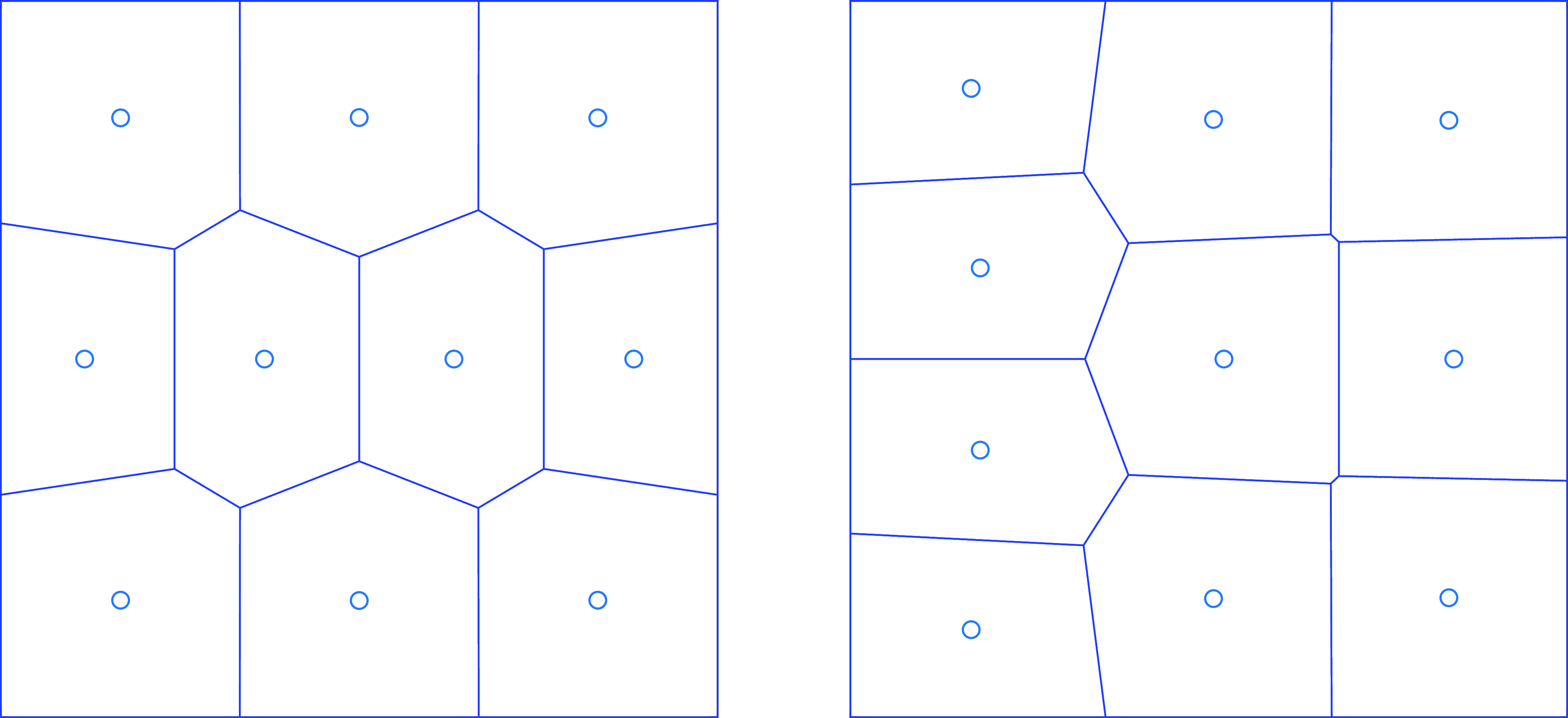
 μ=1
μ=1 Vi
Vi xi
xi J
J ν=∑i=110miδxi
 μ
μ mi
mi xi
xi
 Ω=[0,L]2
 L=5
L=5 M=4
M=4 (x1,x2,x3,x4)=L⋅((0.375,0.375),(0.75,0.35),
 (0.65,0.75),(0.25,0.8))
 (m1,m2,m3,m4)=|Ω|⋅(0.38,0.29,0.19,0.14)
 {Ci(w)}i=1M
 R
R (x1,…,xM)
 ρ
ρ dρdμ(x)=0
 {Ci(w)}i=1M
 c(x,y)=[d(x,y)/2]2
 c(x,y)=d(x,y)2
 sptρ
sptρ Ci(w)
Ci(w)
 [0,L]×{0.375L}
 L=5
L=5 ϕw
ϕw w∈RM
w∈RM ϕw
ϕw cHK
cHK ϕw=∞
ϕw=∞ R≠∅
R≠∅ dρdμ
dρdμ dρdμ=(F∗)′(−ϕw)
 Ω∖R
Ω∖R 0
0 cos(d(y,xi))2
 Ω∖R
Ω∖R 0
0 R
R
 Ω=[0,1]2
 xi/L
xi/L mi/|Ω|
 ε
ε {Ci(w)}i=1M
 R
R (x1,…,xM)
 ρ
ρ ε
ε ε
ε
 Ω=[0,1]2
 ε
ε M=128
M=128 Ci(w)
Ci(w) i
i ε
ε Ci(w)
Ci(w) xi
xi ε
ε Ci(w)
Ci(w) Bεπ/2(xi)
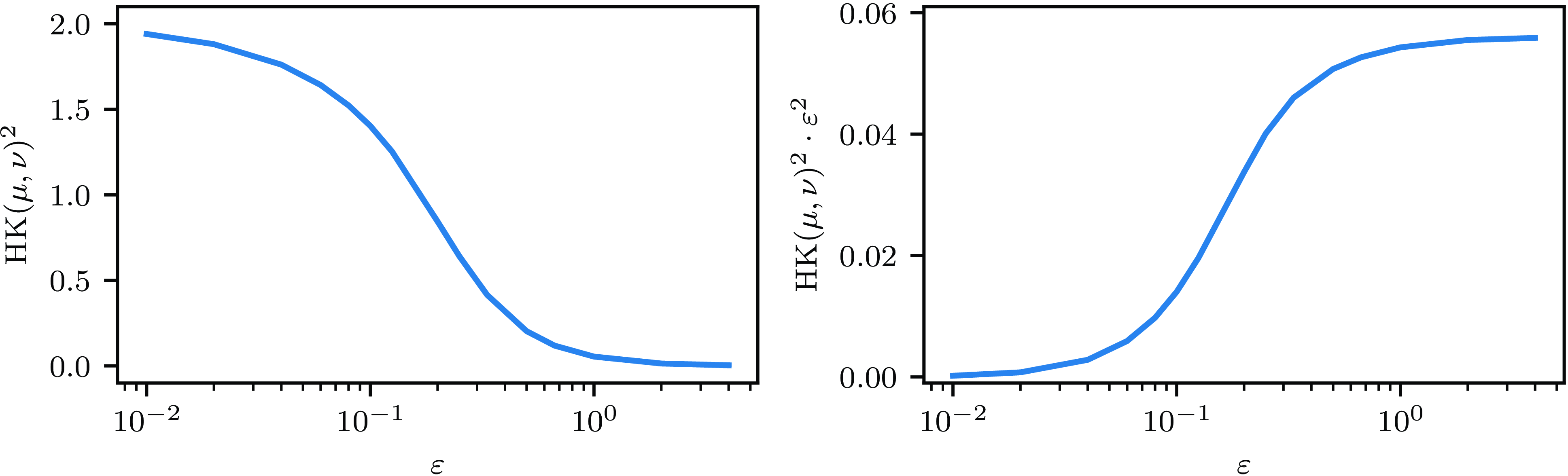
 HKε(μ,ν)2
 ε
ε ε↘0
ε↘0 HKε(μ,ν)2
 Hell(μ,ν)2=2
 ε→∞
ε→∞ ε2HKε(μ,ν)2
 W2(μ,ν)2
 μ
μ (x1,…,xM)
 M=100
M=100 μ
μ
 μ=(1+exp(−|x|22(4π)2))⋅L⌞Ω
 Ω=[−4π,4π]2
 M=16
M=16 x1,…,xM
 {Vi(x1,…,xM)}i=1M
 ρ=π1#γ
 dρdμ(x)=0
 ρ=μ
ρ=μ
 Ci(0)
Ci(0) R
R ρ=π1#γ
 μ
μ
 εM2M
εM2M ρ=π1#γ
 μ
μ
 B′
B′ μ
μ D
D P=limM→∞εM2M
 0
0
 Open access