


1 Introduction
Let M be a compact d-manifold. Let $\sqsubset $
denote
$\sqsubset $
denote $(M \times \{0\}) \cup (\partial M \times [0,1]) \subseteq M \times [0,1]$
. A pseudo-isotopy of M is a homeomorphism
$(M \times \{0\}) \cup (\partial M \times [0,1]) \subseteq M \times [0,1]$
. A pseudo-isotopy of M is a homeomorphism $F \colon M \times [0,1] \to M \times [0,1]$
such that
$F \colon M \times [0,1] \to M \times [0,1]$
such that $F|_{\sqsubset } = \operatorname {Id}_{\sqsubset }$
. The homeomorphism
$F|_{\sqsubset } = \operatorname {Id}_{\sqsubset }$
. The homeomorphism $f \colon M \to M$
obtained from restricting F to
$f \colon M \to M$
obtained from restricting F to $M \times \{1\}$
is said to be pseudo-isotopic to the identity. If F is level-preserving, i.e. if
$M \times \{1\}$
is said to be pseudo-isotopic to the identity. If F is level-preserving, i.e. if $F|_{M \times \{t\}}$
is a homeomorphism from
$F|_{M \times \{t\}}$
is a homeomorphism from $M \times \{t\}$
to itself for all
$M \times \{t\}$
to itself for all $t \in [0,1]$
, then F is the trace of an isotopy; for brevity in this case we refer to F simply as an isotopy. Observe that if F is an isotopy then F is isotopic rel.
$t \in [0,1]$
, then F is the trace of an isotopy; for brevity in this case we refer to F simply as an isotopy. Observe that if F is an isotopy then F is isotopic rel. $\sqsubset $
to the identity map of
$\sqsubset $
to the identity map of $M \times [0,1]$
, and in particular f is isotopic to the identity map of M. There are directly analogous definitions in the smooth and
$M \times [0,1]$
, and in particular f is isotopic to the identity map of M. There are directly analogous definitions in the smooth and $\operatorname {\mathrm {PL}}$
categories.
$\operatorname {\mathrm {PL}}$
categories.
For M smooth and simply-connected, F a diffeomorphism, and $d \geq 5$
, Cerf [Reference CerfCer70] proved that F is smoothly isotopic to the identity, which in particular implies that f is smoothly isotopic to the identity. For
$d \geq 5$
, Cerf [Reference CerfCer70] proved that F is smoothly isotopic to the identity, which in particular implies that f is smoothly isotopic to the identity. For $d \geq 6$
, Cerf’s method was extended by Hatcher–Wagoner [Reference Hatcher and WagonerHW73] and Igusa [Reference IgusaIgu84] to a two-stage obstruction theory deciding in the non-simply-connected setting whether F is smoothly isotopic to the identity. Cerf and Hatcher–Wagoner’s results were extended to the topological and
$d \geq 6$
, Cerf’s method was extended by Hatcher–Wagoner [Reference Hatcher and WagonerHW73] and Igusa [Reference IgusaIgu84] to a two-stage obstruction theory deciding in the non-simply-connected setting whether F is smoothly isotopic to the identity. Cerf and Hatcher–Wagoner’s results were extended to the topological and $\operatorname {\mathrm {PL}}$
categories by Pedersen [Reference Burghelea, Lashof and RothenbergBLR75, Appendix 2], making use of work of Hudson [Reference HudsonHud70] and [Reference PedersenPed77]. The case
$\operatorname {\mathrm {PL}}$
categories by Pedersen [Reference Burghelea, Lashof and RothenbergBLR75, Appendix 2], making use of work of Hudson [Reference HudsonHud70] and [Reference PedersenPed77]. The case $d=5$
in the non-simply-connected case is open at the time of writing, in all categories.
$d=5$
in the non-simply-connected case is open at the time of writing, in all categories.
This article concerns the extension of Cerf’s theorem to dimension four, in the topological category and in the smooth category after stabilising $M \times [0,1]$
with copies of
$M \times [0,1]$
with copies of $S^2 \times S^2 \times [0,1]$
. From now on we set
$S^2 \times S^2 \times [0,1]$
. From now on we set $d=4$
.
$d=4$
.
1.1 Stable isotopy
First we discuss the smooth stable version. We recall the definition of a stable isotopy. Assume that M is a compact, smooth, simply-connected 4-manifold, and that $F \colon M \times [0,1] \to M \times [0,1]$
is a smooth pseudo-isotopy. After an isotopy, we may assume that there is a 4-ball
$F \colon M \times [0,1] \to M \times [0,1]$
is a smooth pseudo-isotopy. After an isotopy, we may assume that there is a 4-ball $D^4 \subseteq M$
such that
$D^4 \subseteq M$
such that $F|_{D^4 \times [0,1]}$
is the identity. We can then connect sum
$F|_{D^4 \times [0,1]}$
is the identity. We can then connect sum $M \times [0,1]$
with
$M \times [0,1]$
with $(\#^k S^2 \times S^2) \times [0,1]$
along
$(\#^k S^2 \times S^2) \times [0,1]$
along $D^4 \times [0,1]$
; let
$D^4 \times [0,1]$
; let $N_k$
denote the result. Consider
$N_k$
denote the result. Consider $F_k\colon N_k\rightarrow N_k$
, extending
$F_k\colon N_k\rightarrow N_k$
, extending $F|_{(M \times [0,1] )\setminus (\mathring {D}^4 \times [0,1])}$
by the identity on
$F|_{(M \times [0,1] )\setminus (\mathring {D}^4 \times [0,1])}$
by the identity on $((\#^k S^2 \times S^2) \times [0,1]) \setminus (\mathring {D}^4 \times [0,1])$
. If there exists a k such that
$((\#^k S^2 \times S^2) \times [0,1]) \setminus (\mathring {D}^4 \times [0,1])$
. If there exists a k such that $F_k$
is smoothly isotopic rel.
$F_k$
is smoothly isotopic rel. $\sqsubset $
to the identity, then we say that the pseudo-isotopy F is stably isotopic to the identity.
$\sqsubset $
to the identity, then we say that the pseudo-isotopy F is stably isotopic to the identity.
Here is Quinn’s $4$
-dimensional smooth stable pseudo-isotopy theorem [Reference QuinnQui86b, Theorem 1.4].
$4$
-dimensional smooth stable pseudo-isotopy theorem [Reference QuinnQui86b, Theorem 1.4].
Theorem 1.1. Let M be a compact, smooth, simply-connected 4-manifold and let $F \colon M \times [0,1] \to M \times [0,1]$
be a smooth pseudo-isotopy. Then F is stably isotopic to the identity.
$F \colon M \times [0,1] \to M \times [0,1]$
be a smooth pseudo-isotopy. Then F is stably isotopic to the identity.
In Section 7 we show that Quinn’s proof of one of the steps in his argument, the Replacement Criterion in [Reference QuinnQui86b, Section 4.5], does not work. We do not know whether the replacement criterion holds, and this is an interesting open question; we state it in Problem 7.1.
The first main goal of this article is to fix Quinn’s proof of Theorem 1.1. We will use the majority of Quinn’s argument, but we modify it to replace his use of the replacement criterion. Our modification uses a method called factorisation, which first appeared in [Reference GabaiGab22, Lemma 3.15], to split a pseudo-isotopy in two; see below Remark 4.3. One of the two resulting pseudo-isotopies can be stably isotoped to the identity using Quinn’s methods. We present a new argument, a novel application of Quinn’s sum square move, to resolve the other pseudo-isotopy. We exploit extra $S^2 \times S^2$
summands to find geometrically dual, framed embedded spheres to certain surfaces, when they are required.
$S^2 \times S^2$
summands to find geometrically dual, framed embedded spheres to certain surfaces, when they are required.
Remark 1.2. Stabilisation is necessary in Theorem 1.1. In dimension 4, smooth pseudo-isotopy does not imply smooth isotopy for 1-connected 4-manifolds, as shown first by Ruberman [Reference RubermanRub98], with later examples constructed by Kronheimer-Mrowka [Reference Kronheimer and MrowkaKM20], Baraglia-Konno [Reference Baraglia and KonnoBK20], Lin [Reference LinLin23], and Konno-Mallick-Taniguchi [Reference Konno, Mallick and TaniguchiKMT23], among others.
Quinn deduced the following result from Theorem 1.1, stated as [Reference QuinnQui86b, Theorem 1.2]. Here $\operatorname {\mathrm {TOP}}(4)$
denotes the topological group of homeomorphisms of
$\operatorname {\mathrm {TOP}}(4)$
denotes the topological group of homeomorphisms of $\mathbb {R}^4$
that fix the origin, and
$\mathbb {R}^4$
that fix the origin, and $\operatorname {\mathrm {TOP}}(4)/\operatorname {\mathrm {O}}(4)$
denotes the homotopy fibre of the canonical map
$\operatorname {\mathrm {TOP}}(4)/\operatorname {\mathrm {O}}(4)$
denotes the homotopy fibre of the canonical map $\operatorname {\mathrm {BO}}(4) \to \operatorname {\mathrm {BTOP}}(4)$
.
$\operatorname {\mathrm {BO}}(4) \to \operatorname {\mathrm {BTOP}}(4)$
.
Theorem 1.3. $\pi _4(\operatorname {\mathrm {TOP}}(4)/\operatorname {\mathrm {O}}(4)) =0$
.
$\pi _4(\operatorname {\mathrm {TOP}}(4)/\operatorname {\mathrm {O}}(4)) =0$
.
The space $\operatorname {\mathrm {TOP}}(4)/\operatorname {\mathrm {O}}(4)$
is an important universal space in smoothing theory. For example, Theorem 1.3 was the final step in showing [Reference Freedman and QuinnFQ90, Theorem 8.7A], that
$\operatorname {\mathrm {TOP}}(4)/\operatorname {\mathrm {O}}(4)$
is an important universal space in smoothing theory. For example, Theorem 1.3 was the final step in showing [Reference Freedman and QuinnFQ90, Theorem 8.7A], that $\operatorname {\mathrm {TOP}}(4)/\operatorname {\mathrm {O}}(4) \to \operatorname {\mathrm {TOP}}/\operatorname {\mathrm {O}}$
is 5-connected. In combination with Lees and Lashof’s immersion theory [Reference LeesLee69, Reference LashofLas70a, Reference LashofLas70b, Reference LashofLas71], this implies [Reference Freedman and QuinnFQ90, Theorem 8.7B], which states that for M a noncompact, connected 4-manifold, concordance classes of smooth structures correspond bijectively with the cohomology group
$\operatorname {\mathrm {TOP}}(4)/\operatorname {\mathrm {O}}(4) \to \operatorname {\mathrm {TOP}}/\operatorname {\mathrm {O}}$
is 5-connected. In combination with Lees and Lashof’s immersion theory [Reference LeesLee69, Reference LashofLas70a, Reference LashofLas70b, Reference LashofLas71], this implies [Reference Freedman and QuinnFQ90, Theorem 8.7B], which states that for M a noncompact, connected 4-manifold, concordance classes of smooth structures correspond bijectively with the cohomology group $H^3(M,\partial M;\mathbb {Z}/2)$
.
$H^3(M,\partial M;\mathbb {Z}/2)$
.
Remark 1.4. There is now an alternative proof due to Gabai [Reference GabaiGab22, Theorem 2.5], of the fact that smoothly pseudo-isotopic diffeomorphisms of a compact 1-connected 4-manifold are stably isotopic. However Gabai’s proof does not trivialise the given pseudo-isotopy, so does not recover Theorem 1.1. Thus Gabai’s theorem [Reference GabaiGab22, Theorem 2.5] cannot be applied to prove Theorem 1.3.
We note that Perron’s article [Reference PerronPer86], which we will discuss more below, did not address Theorem 1.1, and it is not clear how to approach it using Perron’s method, due to his use of the Alexander trick. Thus as far as we know Theorem 1.3 cannot be deduced from Perron’s work.
The only proof known to us of Theorem 1.3 makes use of our corrected proof of Theorem 1.1.
1.2 Topological isotopy
Now we discuss the topological 4-dimensional analogue of Cerf’s theorem.
Theorem 1.5. Let M be a compact, topological, 1-connected 4-manifold and let $F \colon M \times [0,1] \to M \times [0,1]$
be a pseudo-isotopy. Then F is topologically isotopic rel.
$F \colon M \times [0,1] \to M \times [0,1]$
be a pseudo-isotopy. Then F is topologically isotopic rel. $\sqsubset $
to the identity
$\sqsubset $
to the identity $\operatorname {Id}_{M \times [0,1]}$
.
$\operatorname {Id}_{M \times [0,1]}$
.
The first proof of Theorem 1.5, for a class of $4$
-manifolds discussed next, was given by Perron [Reference PerronPer86]. Perron’s main result states the theorem for smooth, compact 4-manifolds without 1-handles. In [Reference PerronPer86, Section 7], Perron deduced the statement for closed, 1-connected, topological 4-manifolds, using an argument he attributes to Siebenmann. In Section 5 we will explain how this deduction can be extended further to compact manifolds with boundary using work of Boyer [Reference BoyerBoy86, Reference BoyerBoy93] to deduce all cases of Theorem 1.5. This extension is necessary because Casson [Reference KirbyKir78, Remarks following Problem 4.18] showed there are compact, contractible, smooth 4-manifolds with boundary that do not admit a handle decomposition with no 1-handles.
$4$
-manifolds discussed next, was given by Perron [Reference PerronPer86]. Perron’s main result states the theorem for smooth, compact 4-manifolds without 1-handles. In [Reference PerronPer86, Section 7], Perron deduced the statement for closed, 1-connected, topological 4-manifolds, using an argument he attributes to Siebenmann. In Section 5 we will explain how this deduction can be extended further to compact manifolds with boundary using work of Boyer [Reference BoyerBoy86, Reference BoyerBoy93] to deduce all cases of Theorem 1.5. This extension is necessary because Casson [Reference KirbyKir78, Remarks following Problem 4.18] showed there are compact, contractible, smooth 4-manifolds with boundary that do not admit a handle decomposition with no 1-handles.
Quinn [Reference QuinnQui86b, Theorem 1.4] gave an independent proof of Theorem 1.5, for all compact, topological, 1-connected 4-manifolds. Quinn’s work may be thought of as a natural extension of Cerf’s approach to dimension $4$
. A (presently unknown) extension to non-simply-connected
$4$
. A (presently unknown) extension to non-simply-connected $4$
-manifolds would likely involve a combination of the higher-dimensional Hatcher–Wagoner theory for nontrivial fundamental groups and a suitable extension of Quinn’s approach.
$4$
-manifolds would likely involve a combination of the higher-dimensional Hatcher–Wagoner theory for nontrivial fundamental groups and a suitable extension of Quinn’s approach.
The second main goal of this article is to fix Quinn’s proof of Theorem 1.5, which also relied on his replacement criterion [Reference QuinnQui86b, Section 4.5]. Thus, given the extension of Perron’s proof to manifolds with boundary, discussed above, and our completion of Quinn’s argument, there are two independent proofs of Theorem 1.5 in full generality. As with the fix of Theorem 1.1, we will retain the majority of Quinn’s argument, however we will again split the given pseudo-isotopy into two using factorisation. One of the resulting pseudo-isotopies can be resolved using Quinn’s argument from [Reference QuinnQui86b, Section 4.6]. For the second we arrange for a judicious application of the Alexander trick.
Remark 1.6. As discussed above, there is a well established obstruction theory for pseudo-isotopies of non-simply-connected manifolds in dimensions $\geq 6$
, in both topological and smooth categories. An analogue of such a theory is not presently known for non-simply-connected
$\geq 6$
, in both topological and smooth categories. An analogue of such a theory is not presently known for non-simply-connected $4$
-manifolds. However, it follows from the work of Budney-Gabai [Reference Budney and GabaiBG25] that the simply-connected hypothesis cannot be removed in Theorem 1.5.
$4$
-manifolds. However, it follows from the work of Budney-Gabai [Reference Budney and GabaiBG25] that the simply-connected hypothesis cannot be removed in Theorem 1.5.
1.3 Classification of homeomorphisms up to isotopy
An important application of Theorem 1.5 is to classify homeomorphisms of 1-connected 4-manifolds up to isotopy. To achieve this one also needs a classification of homeomorphisms up to pseudo-isotopy.
The classification of diffeomorphisms up to smooth pseudo-isotopy was done using modified surgery by Kreck [Reference KreckKre79] for closed, smooth, 1-connected 4-manifolds. Quinn gave the classification for homeomorphisms of closed, topological, 1-connected 4-manifolds in [Reference QuinnQui86b], with a correction of the analysis of the normal invariants given by Cochran-Habegger [Reference Cochran and HabeggerCH90]. It is also straightforward to adapt Kreck’s argument to the topological category.
The outcome [Reference QuinnQui86b, Theorem 1.1] of the classification of homeomorphisms up to pseudo-isotopy, combined with Theorem 1.5, is that the natural map
 $$\begin{align*}\pi_0\operatorname{\mathrm{Homeo}}^+(M) \xrightarrow{\cong} \operatorname{\mathrm{Aut}}(H_2(M),\lambda_M),\end{align*}$$
sending an isotopy classes of orientation-preserving homeomorphisms of M to the induced isometry of the intersection pairing $\lambda _M \colon H_2(M) \times H_2(M) \to \mathbb {Z}$
, is an isomorphism. Surjectivity is due to Freedman [Reference FreedmanFre82].
$\lambda _M \colon H_2(M) \times H_2(M) \to \mathbb {Z}$
, is an isomorphism. Surjectivity is due to Freedman [Reference FreedmanFre82].
For homeomorphisms of compact, 1-connected, topological manifolds, with possibly nonempty boundary, the classification up to pseudo-isotopy, and hence up to isotopy by Theorem 1.5, was completed by Orson-Powell [Reference Orson and PowellOP25]. The corresponding surjectivity result in the case of nonempty boundary is due to Boyer [Reference BoyerBoy86].
Organisation
We begin by explaining our remedy for the proof of Theorem 1.1. In Section 2 we recall the start of Quinn’s proof in the smooth setting, and state the key propositions from his paper that we will use. Section 3 recalls two key geometric constructions: Whitney spheres and the sum square move. Section 4 contains the details of our fix for the proof of Theorem 1.1.
Section 5 proves a key lemma on a decomposition of compact 1-connected topological 4-manifolds. It has two aims. It gives a key input for Quinn’s topological approach, and it enables us to explain how Perron’s method can be applied to all compact 1-connected 4-manifolds, and not just those that are either closed or admit a handle decomposition without 1-handles.
In Section 6 we adapt our fix from Section 4 to the topological case. Finally, in Section 7 we give more details on the problem with Quinn’s proof of the Replacement Criterion, and pose the question of whether the replacement lemma holds.
2 Morse functions, nested eye Cerf graphics, and the start of Quinn’s proof
In this section we summarise the start of Quinn’s proof assuming the input of a smooth pseudo-isotopy. We explain the position one is in prior to Quinn’s use of the replacement criterion, and to set up notation. After the replacement criterion, Quinn’s argument for completing the stable smooth proof is also valid, and we make use of this too, in the form of Theorem 2.3 below.
Throughout this section and Section 4 we work in the smooth category. In Sections 5 and 6 we will explain how to adapt the arguments to the topological category, unstably.
A smooth pseudo-isotopy $F \colon M \times [0,1] \to M \times [0,1]$
of a smooth compact 1-connected 4-manifold can be translated into a 1-parameter family of generalised Morse functions
$F \colon M \times [0,1] \to M \times [0,1]$
of a smooth compact 1-connected 4-manifold can be translated into a 1-parameter family of generalised Morse functions $G_t \colon M \times [0,1] \to [0,1]$
, where
$G_t \colon M \times [0,1] \to [0,1]$
, where $G_0 = \operatorname {\mathrm {pr}}_2$
and
$G_0 = \operatorname {\mathrm {pr}}_2$
and $G_1 = \operatorname {\mathrm {pr}}_2 \circ F$
. Here
$G_1 = \operatorname {\mathrm {pr}}_2 \circ F$
. Here $\operatorname {\mathrm {pr}}_2$
denotes projection onto the second factor, namely
$\operatorname {\mathrm {pr}}_2$
denotes projection onto the second factor, namely $[0,1]$
. Both
$[0,1]$
. Both $G_0$
and
$G_0$
and $G_1$
have no critical points. The family
$G_1$
have no critical points. The family $G_t$
is also accompanied by a 1-parameter family of gradient-like vector fields
$G_t$
is also accompanied by a 1-parameter family of gradient-like vector fields $\xi _t$
subordinate to
$\xi _t$
subordinate to $G_t$
.
$G_t$
.
Given a pair $(G_t,\xi _t)$
, one can in turn recover a pseudo-isotopy
$(G_t,\xi _t)$
, one can in turn recover a pseudo-isotopy $F \colon M\times [0,1] \to M \times [0,1]$
. The proof of the fact that pseudo-isotopy implies isotopy consists of deformations of these 1-parameter families, i.e. a 1-parameter family of 1-parameter families. A deformation corresponds to an isotopy of the pseudo-isotopy F. The aim is to deform
$F \colon M\times [0,1] \to M \times [0,1]$
. The proof of the fact that pseudo-isotopy implies isotopy consists of deformations of these 1-parameter families, i.e. a 1-parameter family of 1-parameter families. A deformation corresponds to an isotopy of the pseudo-isotopy F. The aim is to deform $(G_t,\xi _t)$
until there are no critical points of
$(G_t,\xi _t)$
until there are no critical points of $G_t$
, for all
$G_t$
, for all $t \in [0,1]$
. Such a 1-parameter family corresponds to a pseudo-isotopy F that is an isotopy.
$t \in [0,1]$
. Such a 1-parameter family corresponds to a pseudo-isotopy F that is an isotopy.
Using $\operatorname {\mathrm {Wh}}_2(\{1\})=\{1\}$
, by the work of Hatcher–Wagoner [Reference Hatcher and WagonerHW73, Chapter VI, Proposition 3] one can arrange by a deformation of the family that the Cerf graphic associated to
$\operatorname {\mathrm {Wh}}_2(\{1\})=\{1\}$
, by the work of Hatcher–Wagoner [Reference Hatcher and WagonerHW73, Chapter VI, Proposition 3] one can arrange by a deformation of the family that the Cerf graphic associated to $G_t$
consists of finitely many nested eyes – pairs of index 2 and 3 critical points that are born near time
$G_t$
consists of finitely many nested eyes – pairs of index 2 and 3 critical points that are born near time $t_b$
, and die at time
$t_b$
, and die at time $t_d> t_b$
, with no rearrangements. More precisely, we let
$t_d> t_b$
, with no rearrangements. More precisely, we let $t_b$
be the time of the final birth, and let
$t_b$
be the time of the final birth, and let $t_d$
be the time of the first death. See Figure 1. According to Hatcher–Wagoner [Reference Hatcher and WagonerHW73, Chapter VI, Proposition 3], we may assume that there are no handle slides, no critical value crossings, and that the births and deaths are independent. In particular, there are no trajectories between any pair of index 3 critical points, and similarly for any pair of index 2 critical points. Moreover at the moment of each birth and shortly thereafter, the index
$t_d$
be the time of the first death. See Figure 1. According to Hatcher–Wagoner [Reference Hatcher and WagonerHW73, Chapter VI, Proposition 3], we may assume that there are no handle slides, no critical value crossings, and that the births and deaths are independent. In particular, there are no trajectories between any pair of index 3 critical points, and similarly for any pair of index 2 critical points. Moreover at the moment of each birth and shortly thereafter, the index $2$
and
$2$
and $3$
critical points that appear do not have trajectories to any other critical points, other than the unique trajectory between them. The same holds at each death, and shortly before.
$3$
critical points that appear do not have trajectories to any other critical points, other than the unique trajectory between them. The same holds at each death, and shortly before.
A family of nested eyes.

If we can ‘close’ the innermost eye in the family of nested eyes, one at a time, then we complete the proof of the smooth stable isotopy theorem. We formalise this in the following inductive hypothesis.
Inductive Hypothesis 2.1 ( $\mathbf {E(n)}$
).
$\mathbf {E(n)}$
).

Let M be a smooth 1-connected 4-manifold and let $(G_t,\xi _t)$
be as above, a 1-parameter family of generalised Morse functions and gradient like vector fields on
$(G_t,\xi _t)$
be as above, a 1-parameter family of generalised Morse functions and gradient like vector fields on $M \times [0,1]$
. Suppose that the associated Cerf graphic consists of n nested eyes with cancelling pairs of index 2 and 3 critical points, with no handle slides. Then after stabilising
$M \times [0,1]$
. Suppose that the associated Cerf graphic consists of n nested eyes with cancelling pairs of index 2 and 3 critical points, with no handle slides. Then after stabilising $M \times [0,1]$
with
$M \times [0,1]$
with $(\#^p S^2 \times S^2) \times [0,1]$
, for some p, there is a deformation of
$(\#^p S^2 \times S^2) \times [0,1]$
, for some p, there is a deformation of $(G_t,\xi _t)$
to a 1-parameter family without critical points.
$(G_t,\xi _t)$
to a 1-parameter family without critical points.
We will prove the base case $E(1)$
and we will deduce the case
$E(1)$
and we will deduce the case $E(n)$
from
$E(n)$
from $E(n-1)$
. The core of Quinn’s proof starts with a nested eye family, and works on the innermost eye. We set up notation and recall the salient points of Quinn’s argument for removing the innermost eye.
$E(n-1)$
. The core of Quinn’s proof starts with a nested eye family, and works on the innermost eye. We set up notation and recall the salient points of Quinn’s argument for removing the innermost eye.
Let us suppose we have a family of n nested eyes, for some $n \geq 1$
. In the level sets
$n \geq 1$
. In the level sets $G_{t}^{-1}(1/2)$
, for
$G_{t}^{-1}(1/2)$
, for $t_b < t< t_d$
, we have a copy of
$t_b < t< t_d$
, we have a copy of $M \#_{i=1}^n S^2 \times S^2$
. For each t we have n spheres
$M \#_{i=1}^n S^2 \times S^2$
. For each t we have n spheres $\{A_i^t\}_{i=1}^n$
, which are the ascending spheres of the index 2 critical points, and n spheres
$\{A_i^t\}_{i=1}^n$
, which are the ascending spheres of the index 2 critical points, and n spheres $\{B_i^t\}_{i=1}^n$
, which are the descending spheres of the index 3 critical points. Shortly after the last birth time
$\{B_i^t\}_{i=1}^n$
, which are the descending spheres of the index 3 critical points. Shortly after the last birth time $t_b$
, the sphere
$t_b$
, the sphere $A_i^t$
is the sphere
$A_i^t$
is the sphere $S^2 \times \{\operatorname {\mathrm {pt}}\}$
in the ith
$S^2 \times \{\operatorname {\mathrm {pt}}\}$
in the ith $S^2 \times S^2$
summand. Similarly the sphere
$S^2 \times S^2$
summand. Similarly the sphere $B_i^t$
is the sphere
$B_i^t$
is the sphere $\{\operatorname {\mathrm {pt}}\} \times S^2$
in the ith
$\{\operatorname {\mathrm {pt}}\} \times S^2$
in the ith $S^2 \times S^2$
summand. The
$S^2 \times S^2$
summand. The $A_i^t$
and the
$A_i^t$
and the $B_i^t$
are enumerated so that
$B_i^t$
are enumerated so that $A_1$
and
$A_1$
and $B_1$
correspond to the innermost eye, and then moving outwards, as shown in e.g. Figure 6. Let
$B_1$
correspond to the innermost eye, and then moving outwards, as shown in e.g. Figure 6. Let $A^{t} := \cup _{i=1}^{n} A_{i}^{t}$
and let
$A^{t} := \cup _{i=1}^{n} A_{i}^{t}$
and let $B^{t} := \cup _{i=1}^{n} B_{i}^{t}$
.
$B^{t} := \cup _{i=1}^{n} B_{i}^{t}$
.
One may specify an identification of $G_{t}^{-1}(1/2)$
with
$G_{t}^{-1}(1/2)$
with $M \#_{i=1}^n S^2 \times S^2$
for all
$M \#_{i=1}^n S^2 \times S^2$
for all $t_b < t< t_d$
. This is implicit in [Reference QuinnQui86b] and described in detail in [Reference Krushkal, Mukherjee, Powell and WarrenKMPW24, Construction 3.1]; see also [Reference GayGay25, Proof of Theorem 9]. Then it makes sense to discuss subsets of
$t_b < t< t_d$
. This is implicit in [Reference QuinnQui86b] and described in detail in [Reference Krushkal, Mukherjee, Powell and WarrenKMPW24, Construction 3.1]; see also [Reference GayGay25, Proof of Theorem 9]. Then it makes sense to discuss subsets of $G_t^{-1}(1/2)$
, for
$G_t^{-1}(1/2)$
, for $t_b < t< t_d$
as being in the fixed manifold
$t_b < t< t_d$
as being in the fixed manifold $M \#_{i=1}^n S^2 \times S^2$
. Following [Reference QuinnQui86b, p. 353], we may consider that
$M \#_{i=1}^n S^2 \times S^2$
. Following [Reference QuinnQui86b, p. 353], we may consider that $A^t$
stays fixed as t varies in
$A^t$
stays fixed as t varies in $t_b <t <t_d$
,
$t_b <t <t_d$
, $B^t$
moves by an isotopy, and
$B^t$
moves by an isotopy, and $A^t \cup B^t$
undergoes a regular homotopy. We may also assume that there are times
$A^t \cup B^t$
undergoes a regular homotopy. We may also assume that there are times $t_f$
and
$t_f$
and $t_w$
, with
$t_w$
, with $t_b < t_f < 1/2 < t_w < t_d$
, such that at time
$t_b < t_f < 1/2 < t_w < t_d$
, such that at time $t_f$
a collection of finger moves occur, and at time
$t_f$
a collection of finger moves occur, and at time $t_w$
a collection of Whitney moves occur. During these moves, intersections of
$t_w$
a collection of Whitney moves occur. During these moves, intersections of $B_j^t$
with
$B_j^t$
with $A_i^t$
are created or removed, respectively. We consider the middle-middle level,
$A_i^t$
are created or removed, respectively. We consider the middle-middle level, $G_{1/2}^{-1}(1/2)$
. We can let the finger and Whitney discs evolve so that we see both simultaneously in the middle-middle level. We write
$G_{1/2}^{-1}(1/2)$
. We can let the finger and Whitney discs evolve so that we see both simultaneously in the middle-middle level. We write $A_i := A_i^{1/2}$
and
$A_i := A_i^{1/2}$
and $B_j := B^{1/2}_j$
; that is, in the middle-middle level we drop the t from the notation.
$B_j := B^{1/2}_j$
; that is, in the middle-middle level we drop the t from the notation.
In the middle-middle level, we call the finger move discs for $A_i$
,
$A_i$
, $B_j$
intersections
$B_j$
intersections $\{V^{ij}_k\}$
, and write
$\{V^{ij}_k\}$
, and write $V^{ij} := \cup _k V^{ij}_k$
. Analogously we call the Whitney discs
$V^{ij} := \cup _k V^{ij}_k$
. Analogously we call the Whitney discs $\{W^{ij}_{\ell }\}$
, and write
$\{W^{ij}_{\ell }\}$
, and write $W^{ij} := \cup _{\ell } W^{ij}_{\ell }$
. We also write
$W^{ij} := \cup _{\ell } W^{ij}_{\ell }$
. We also write $V := \cup _{i,j} V^{ij}$
and
$V := \cup _{i,j} V^{ij}$
and $W := \cup _{i,j} W^{ij}$
.
$W := \cup _{i,j} W^{ij}$
.
A Cerf family $(G_t,\xi _t)$
, up to deformation, determines and is determined by the data
$(G_t,\xi _t)$
, up to deformation, determines and is determined by the data $(A,B,V,W)$
in
$(A,B,V,W)$
in $M \#_{i=1}^n S^2 \times S^2$
. This is implicit in [Reference QuinnQui86b]; a detailed discussion is given in [Reference Krushkal, Mukherjee, Powell and WarrenKMPW24, Section 3.1]. One of Quinn’s insights was to describe modifications of this data that correspond to deformations of the family
$M \#_{i=1}^n S^2 \times S^2$
. This is implicit in [Reference QuinnQui86b]; a detailed discussion is given in [Reference Krushkal, Mukherjee, Powell and WarrenKMPW24, Section 3.1]. One of Quinn’s insights was to describe modifications of this data that correspond to deformations of the family $(G_t,\xi _t)$
. The idea of his proof is to start with
$(G_t,\xi _t)$
. The idea of his proof is to start with $(G_t,\xi _t)$
, consider the corresponding
$(G_t,\xi _t)$
, consider the corresponding $(A,B,V,W)$
, suitably modify them, and then deduce that
$(A,B,V,W)$
, suitably modify them, and then deduce that $(G_t,\xi _t)$
can be deformed to a Cerf family without critical points.
$(G_t,\xi _t)$
can be deformed to a Cerf family without critical points.
Working on the innermost eye, Quinn showed in [Reference QuinnQui86b, Sections 4.2–4.4] that we can assume, after a deformation, that both
 $$\begin{align*}\big(\bigcup_k \partial V^{11}_k \cup \partial W^{11}_k\big) \cap A_1\end{align*}$$
and
 $$\begin{align*}\big(\bigcup_k \partial V^{11}_k \cup \partial W^{11}_k\big) \cap B_1\end{align*}$$
are arcs in $A_1$
and
$A_1$
and $B_1$
respectively. We will refer to this as Quinn’s arc condition. See Figure 2.
$B_1$
respectively. We will refer to this as Quinn’s arc condition. See Figure 2.
Convention 2.2. We will assume that the finger and Whitney discs, $\{ V^{11}_k\}$
and
$\{ V^{11}_k\}$
and $\{ W^{11}_l\}$
, for the intersections in the innermost eye, are indexed according to their order in the arc, as indicated in Figure 2.
$\{ W^{11}_l\}$
, for the intersections in the innermost eye, are indexed according to their order in the arc, as indicated in Figure 2.
Finger and Whitney discs with boundaries forming an arc in $A_1$
and in
$A_1$
and in $B_1$
. The Whitney spheres from Section 3.1 corresponding to the finger move discs are also shown.
$B_1$
. The Whitney spheres from Section 3.1 corresponding to the finger move discs are also shown.

For a disc D, let $\mathring D$
denote its interior. The following statement summarises the result of [Reference QuinnQui86b, Section 4.6].
$\mathring D$
denote its interior. The following statement summarises the result of [Reference QuinnQui86b, Section 4.6].
Theorem 2.3 (Quinn).
Suppose that M is smooth, compact, and 1-connected, and suppose that $F \colon M \times [0,1] \xrightarrow {\cong } M \times [0,1]$
is a smooth pseudo-isotopy. Consider an associated 1-parameter family
$F \colon M \times [0,1] \xrightarrow {\cong } M \times [0,1]$
is a smooth pseudo-isotopy. Consider an associated 1-parameter family $(G_t,\xi _t)$
, and suppose that the associated Cerf graphic consists of n nested eyes with cancelling pairs of index 2 and 3 critical points, and no handle slides. Consider the data of spheres and finger/Whitney discs
$(G_t,\xi _t)$
, and suppose that the associated Cerf graphic consists of n nested eyes with cancelling pairs of index 2 and 3 critical points, and no handle slides. Consider the data of spheres and finger/Whitney discs $(A,B,V,W)$
in the middle-middle level.
$(A,B,V,W)$
in the middle-middle level.
If Quinn’s arc condition is satisfied for $(A,B,V,W)$
, and if the algebraic intersection numbers
$(A,B,V,W)$
, and if the algebraic intersection numbers $\mathring {V}^{11}_k \cdot \mathring {W}^{11}_{\ell }$
vanish for all
$\mathring {V}^{11}_k \cdot \mathring {W}^{11}_{\ell }$
vanish for all $k,\ell $
, then after stabilisation of the pseudo-isotopy with
$k,\ell $
, then after stabilisation of the pseudo-isotopy with $(\#^p S^2 \times S^2) \times [0,1]$
, for some p, there is a smooth deformation of the family to one with
$(\#^p S^2 \times S^2) \times [0,1]$
, for some p, there is a smooth deformation of the family to one with $(n-1)$
nested eyes.
$(n-1)$
nested eyes.
Quinn used the problematic replacement criterion to arrange for the algebraic intersection condition in Theorem 2.3 to hold. Since we cannot appeal to the replacement criterion, we must provide an alternative argument.
3 Whitney spheres and the sum square move
Here we take a short digression to recall two important constructions that we shall need in Section 4. In Section 3.1 we recall the construction of Whitney spheres. In Section 3.2 we recall Quinn’s sum square move.
3.1 Whitney spheres
We recall a construction of the Whitney sphere $S_{V_k^{ij}}$
associated with a finger move disc
$S_{V_k^{ij}}$
associated with a finger move disc $V_k^{ij}$
. These spheres have appeared in different guises in the literature, cf. [Reference QuinnQui86b, Section 4.3], [Reference Freedman and QuinnFQ90, Section 3.1, Ex. (2)], [Reference Cha, Orr and PowellCOP20, Section 4.2], [Reference Schneiderman and TeichnerST19, Section 2]. We use the terminology and the description from [Reference Schneiderman and TeichnerST19].
$V_k^{ij}$
. These spheres have appeared in different guises in the literature, cf. [Reference QuinnQui86b, Section 4.3], [Reference Freedman and QuinnFQ90, Section 3.1, Ex. (2)], [Reference Cha, Orr and PowellCOP20, Section 4.2], [Reference Schneiderman and TeichnerST19, Section 2]. We use the terminology and the description from [Reference Schneiderman and TeichnerST19].
The description is given in ${\mathbb R}^3\times {\mathbb R}$
where
${\mathbb R}^3\times {\mathbb R}$
where $A_i$
and the finger disc
$A_i$
and the finger disc $V_k^{ij}$
are in
$V_k^{ij}$
are in ${\mathbb R}^3\times \{0\}$
, and
${\mathbb R}^3\times \{0\}$
, and $B_j$
is represented as (arc
$B_j$
is represented as (arc $\subseteq {\mathbb R}^3$
)
$\subseteq {\mathbb R}^3$
) $\times [-1,1]$
, in Figure 3. The Whitney sphere is drawn red, and it consists of two discs,
$\times [-1,1]$
, in Figure 3. The Whitney sphere is drawn red, and it consists of two discs, $D_{i}\subseteq {\mathbb R}^3\times \{ i\}$
,
$D_{i}\subseteq {\mathbb R}^3\times \{ i\}$
, $i=-1,1$
, joined by an annulus (circle
$i=-1,1$
, joined by an annulus (circle $\subseteq {\mathbb R}^3$
)
$\subseteq {\mathbb R}^3$
) $\times [-1,1]$
. Each
$\times [-1,1]$
. Each $D_i$
is constructed using two copies of the finger move disc
$D_i$
is constructed using two copies of the finger move disc $V_k^{ij}$
, so overall the Whitney sphere contains four pushed-off copies of
$V_k^{ij}$
, so overall the Whitney sphere contains four pushed-off copies of $V_k^{ij}$
.
$V_k^{ij}$
.
A description of the Whitney sphere $S_{V_k^{ij}}$
in
$S_{V_k^{ij}}$
in $\mathbb {R}^3\times \mathbb {R}$
.
$\mathbb {R}^3\times \mathbb {R}$
.

The Whitney sphere is framed and embedded and can be assumed to lie in an arbitrarily small neighbourhood of $V_k^{ij}$
.
$V_k^{ij}$
.
3.2 The sum square move
We recall Quinn’s sum square move [Reference QuinnQui86b, Section 4.2], which can be used to modify finger or Whitney disc configurations by a deformation of the pseudo-isotopy. The data for the move is a framed embedded square S in the middle-middle level, with interior disjoint from the spheres A and B, and from the discs V. The square has two edges on the V discs, denoted $V_0$
and
$V_0$
and $V_i$
(anticipating the proof below) in Figure 4, one edge on A, and one on B. New V discs are obtained by cutting
$V_i$
(anticipating the proof below) in Figure 4, one edge on A, and one on B. New V discs are obtained by cutting $V_0, V_i$
along the boundary edges of the sum square S, and gluing in two parallel copies of S. The effect of the move on the boundaries of the discs, on A and B spheres, is illustrated in Figure 7.
$V_0, V_i$
along the boundary edges of the sum square S, and gluing in two parallel copies of S. The effect of the move on the boundaries of the discs, on A and B spheres, is illustrated in Figure 7.
The sum square move.

Figure 4 is a $3$
-dimensional model for the sum square. Here
$3$
-dimensional model for the sum square. Here $A, V_0, V_i$
, and a neighbourhood of the arc of
$A, V_0, V_i$
, and a neighbourhood of the arc of $\partial S$
in B are pictured in the ‘present’,
$\partial S$
in B are pictured in the ‘present’, ${\mathbb R}^3\times \{ 0\}\subseteq {\mathbb R}^3\times {\mathbb R}$
. The rest of B extends into the past and the future. The framing of S along its boundary is determined in the
${\mathbb R}^3\times \{ 0\}\subseteq {\mathbb R}^3\times {\mathbb R}$
. The rest of B extends into the past and the future. The framing of S along its boundary is determined in the $3$
-dimensional model by a nonvanishing vector field on
$3$
-dimensional model by a nonvanishing vector field on $\partial S$
which is normal to S and tangent to
$\partial S$
which is normal to S and tangent to $A, B$
and the V discs; this framing has to admit an extension over S for the move to give rise to embedded V discs.
$A, B$
and the V discs; this framing has to admit an extension over S for the move to give rise to embedded V discs.
A justification is given in [Reference QuinnQui86b, Section 4.2] for why the sum square move gives a deformation of the pseudo-isotopy. As usual in the subject, given the boundary data $\partial S$
, the challenge is to find a framed, embedded S disjoint from other given surfaces. The proof in Section 4 below explains how to achieve this in relevant situations in the stable setting. Note that if
$\partial S$
, the challenge is to find a framed, embedded S disjoint from other given surfaces. The proof in Section 4 below explains how to achieve this in relevant situations in the stable setting. Note that if $S \cap W = \emptyset $
, then the V discs do not acquire new intersections with W as a result of this move.
$S \cap W = \emptyset $
, then the V discs do not acquire new intersections with W as a result of this move.
4 The proof of the inductive step
We continue with the notation and setup from Section 2, and describe our correction to Quinn’s proof of Theorem 1.1.
Suppose that there are m finger discs $\{V^{11}_k\}_{k=1}^m$
. Then there are also m Whitney discs
$\{V^{11}_k\}_{k=1}^m$
. Then there are also m Whitney discs $\{W^{11}_{\ell }\}_{\ell =1}^m$
for
$\{W^{11}_{\ell }\}_{\ell =1}^m$
for $A_1$
–
$A_1$
– $B_1$
intersections. We fix an orientation on each of these discs. Define
$B_1$
intersections. We fix an orientation on each of these discs. Define
 $$\begin{align*}T_{\ell} := \#_{k=\ell}^m S_{V^{11}_k},\end{align*}$$
where the connected sum is formed by tubing the Whitney spheres $S_{V^{11}_k}$
together along arcs in the
$S_{V^{11}_k}$
together along arcs in the $W^{11}_{k}$
that are parallel to one of the boundary arcs of
$W^{11}_{k}$
that are parallel to one of the boundary arcs of $W^{11}_{k}$
, for
$W^{11}_{k}$
, for $k>\ell $
. (The tubing could be done along any arcs, not necessarily arcs in the Whitney discs; generally this would result in algebraically cancelling pairs of intersections which are fine for the applications below.)
$k>\ell $
. (The tubing could be done along any arcs, not necessarily arcs in the Whitney discs; generally this would result in algebraically cancelling pairs of intersections which are fine for the applications below.)
Lemma 4.1. The spheres $\{T_{\ell }\}_{\ell =1}^m$
are mutually disjoint, framed, and embedded in the complement of
$\{T_{\ell }\}_{\ell =1}^m$
are mutually disjoint, framed, and embedded in the complement of $A \cup B \cup V$
. For some choice of orientations on the
$A \cup B \cup V$
. For some choice of orientations on the $T_{\ell }$
we have algebraic intersection numbers
$T_{\ell }$
we have algebraic intersection numbers $T_{\ell } \cdot W^{11}_k = \delta _{k\ell }$
. That is, the collection
$T_{\ell } \cdot W^{11}_k = \delta _{k\ell }$
. That is, the collection $\{T_\ell \}$
forms a collection of algebraically dual spheres to the Whitney discs
$\{T_\ell \}$
forms a collection of algebraically dual spheres to the Whitney discs $\{W^{11}_k\}$
.
$\{W^{11}_k\}$
.
Proof. The $\delta _{k\ell }$
terms can be seen in Figure 2. Each intersection of
$\delta _{k\ell }$
terms can be seen in Figure 2. Each intersection of $\mathring {V}^{11}_{\ell }$
with
$\mathring {V}^{11}_{\ell }$
with $\mathring {W}^{11}_k$
gives rise to four intersections between
$\mathring {W}^{11}_k$
gives rise to four intersections between $S_{{V}^{11}_\ell }$
and
$S_{{V}^{11}_\ell }$
and $\mathring {W}^{11}_k$
. These come in algebraically cancelling pairs, so do not contribute to the intersection numbers in the statement of the lemma.
$\mathring {W}^{11}_k$
. These come in algebraically cancelling pairs, so do not contribute to the intersection numbers in the statement of the lemma.
We write
 $$\begin{align*}J_{kp} := - \mathring{V}^{11}_{k} \cdot \mathring{W}^{11}_{p} \in \mathbb{Z}\end{align*}$$
and let
 $$\begin{align*}\Sigma_{kp} := \#^{J_{kp}} T_{p}\end{align*}$$
denote $J_{kp}$
mutually disjoint parallel, oriented copies of
$J_{kp}$
mutually disjoint parallel, oriented copies of $T_{p}$
, tubed together by annuli contained in a regular neighbourhood of
$T_{p}$
, tubed together by annuli contained in a regular neighbourhood of $T_{p}$
that are disjoint from A, B, V, and W. The spheres
$T_{p}$
that are disjoint from A, B, V, and W. The spheres $\Sigma _{kp}$
are mutually disjoint, framed, and embedded in the complement of
$\Sigma _{kp}$
are mutually disjoint, framed, and embedded in the complement of $A \cup B \cup V$
. Note that
$A \cup B \cup V$
. Note that
 $$\begin{align*}\mathring{W}_{\ell}^{11} \cdot \Sigma_{kp} = \mathring{W}_{\ell}^{11} \cdot \#^{J_{kp}} T_{p} = J_{kp} \delta_{p\ell} = - (\mathring{V}^{11}_{k} \cdot \mathring{W}^{11}_{p})\delta_{p\ell}.\end{align*}$$
Now we want to create a new family of discs whose interiors have trivial algebraic intersection numbers with the interior of every disc $W^{11}_{\ell }$
. We define
$W^{11}_{\ell }$
. We define
 $$\begin{align*}\widetilde{V}^{11}_k := V^{11}_k \#_{p=1}^m \Sigma_{kp}.\end{align*}$$
Note that after a small isotopy, the interiors of discs $\{ \widetilde {V}^{11}_k\}$
may be assumed to be disjoint from the interiors of
$\{ \widetilde {V}^{11}_k\}$
may be assumed to be disjoint from the interiors of $\{ {V}^{11}_k\}$
. We compute
$\{ {V}^{11}_k\}$
. We compute
 $$ \begin{align} \begin{split} \widetilde{V}^{11}_k \cdot \mathring{W}^{11}_{\ell} &= \mathring{V}^{11}_k \cdot \mathring{W}^{11}_{\ell} + \sum_{p=1}^m \Sigma_{kp} \cdot \mathring{W}^{11}_{\ell} \\ &= \mathring{V}^{11}_k \cdot \mathring{W}^{11}_{\ell} - \sum_{p=1}^m (\mathring{V}^{11}_{k} \cdot \mathring{W}^{11}_{p})\delta_{p\ell} \\ &= \mathring{V}^{11}_k \cdot \mathring{W}^{11}_{\ell} - \mathring{V}^{11}_{k} \cdot \mathring{W}^{11}_{\ell} =0. \end{split} \end{align} $$
Finally, for each k we define
 $$\begin{align*}\widehat{V}^{ij}_k := \begin{cases} \widetilde{V}^{11}_k & (i,j) = (1,1) \\ V^{ij}_k & (i,j) \neq (1,1). \end{cases}\end{align*}$$
That is, we replace the discs associated with the innermost eye, but leave all other discs in $\{V^{ij}_k\}$
unchanged. As we explain below, the new family of discs
$\{V^{ij}_k\}$
unchanged. As we explain below, the new family of discs $\{ \widehat {V}^{ij}_k\}$
will be used to factorize the given pseudo-isotopy into two, which we can then trivialize separately.
$\{ \widehat {V}^{ij}_k\}$
will be used to factorize the given pseudo-isotopy into two, which we can then trivialize separately.
Lemma 4.2. The discs $\widehat {V}^{ij}_k$
are pairwise disjoint, framed, and embedded.
$\widehat {V}^{ij}_k$
are pairwise disjoint, framed, and embedded.
Proof. Each of the $\widetilde {V}^{11}_k$
discs lives in a regular neighbourhood of the discs
$\widetilde {V}^{11}_k$
discs lives in a regular neighbourhood of the discs $V^{11}$
, together with arcs on
$V^{11}$
, together with arcs on $A_1$
, say, given by
$A_1$
, say, given by $\partial W^{11} \cap A_1$
. Since the interiors of the boundary arcs of
$\partial W^{11} \cap A_1$
. Since the interiors of the boundary arcs of $V^{11}$
and of
$V^{11}$
and of $W^{11}$
are disjoint by Quinn’s arc condition, and since the
$W^{11}$
are disjoint by Quinn’s arc condition, and since the $V^{ij}$
discs can be assumed to miss a regular neighbourhood of
$V^{ij}$
discs can be assumed to miss a regular neighbourhood of $V^{11}$
, we do not create extra intersections. Also note that the spheres
$V^{11}$
, we do not create extra intersections. Also note that the spheres $\Sigma _{kp}$
are framed, mutually disjoint, disjoint from all
$\Sigma _{kp}$
are framed, mutually disjoint, disjoint from all $\{ {V}^{ij}_k \}$
, and embedded. Hence tubing into them again yields framed and embedded finger discs.
$\{ {V}^{ij}_k \}$
, and embedded. Hence tubing into them again yields framed and embedded finger discs.
Next we will use the freedom to introduce additional $S^2\times S^2$
summands by stabilising the pseudo-isotopy with
$S^2\times S^2$
summands by stabilising the pseudo-isotopy with $(\#^m S^2 \times S^2) \times [0,1]$
. In particular such an operation introduces m additional
$(\#^m S^2 \times S^2) \times [0,1]$
. In particular such an operation introduces m additional $ S^2 \times S^2$
summands into the middle-middle level. This paragraph is specific to the stable proof. The crucial feature of
$ S^2 \times S^2$
summands into the middle-middle level. This paragraph is specific to the stable proof. The crucial feature of $\widehat V^{11}$
is that the algebraic intersection numbers between the components of
$\widehat V^{11}$
is that the algebraic intersection numbers between the components of $\widehat V^{11}$
and the components of
$\widehat V^{11}$
and the components of $W^{11}$
are all zero. We are free to modify
$W^{11}$
are all zero. We are free to modify $\widehat V^{11}$
as long as they continue satisfying this condition and Lemma 4.2 continues to be satisfied. We take
$\widehat V^{11}$
as long as they continue satisfying this condition and Lemma 4.2 continues to be satisfied. We take $\widehat V^{11}$
as defined above, and tube each component into
$\widehat V^{11}$
as defined above, and tube each component into $S^2\times \{\operatorname {\mathrm {pt}}\}$
in its own newly added
$S^2\times \{\operatorname {\mathrm {pt}}\}$
in its own newly added $S^2\times S^2$
summand. Since
$S^2\times S^2$
summand. Since $\widehat V^{11}$
consists of m discs, we add
$\widehat V^{11}$
consists of m discs, we add $m S^2 \times S^2$
summands. Now, in the stabilised middle-middle level, the entire collection of discs
$m S^2 \times S^2$
summands. Now, in the stabilised middle-middle level, the entire collection of discs $\widehat V^{11}$
has a geometrically dual collection of framed embedded spheres that are disjoint from
$\widehat V^{11}$
has a geometrically dual collection of framed embedded spheres that are disjoint from $A \cup B \cup W \cup (V \setminus V^{11})$
.
$A \cup B \cup W \cup (V \setminus V^{11})$
.
Remark 4.3. We have structured the proof so that the steps that use stabilisation by copies of $(S^2 \times S^2) \times [0,1]$
are separated from the rest of the proof. This is a device to avoid having to repeat text verbatim during the topological proof in Section 6.
$(S^2 \times S^2) \times [0,1]$
are separated from the rest of the proof. This is a device to avoid having to repeat text verbatim during the topological proof in Section 6.
Now we perform factorisation [Reference GabaiGab22, Lemma 3.15]. That is, we introduce ex nihilo a cancelling finger-Whitney pair. To explain this we introduce some notation. If we have a finger disc $V_k$
, and we use it as a Whitney disc, then we write it as
$V_k$
, and we use it as a Whitney disc, then we write it as $\underline {V_k}$
, to indicate the same disc in the middle-middle level, but with its modus operandi altered. Analogously if we have a Whitney disc
$\underline {V_k}$
, to indicate the same disc in the middle-middle level, but with its modus operandi altered. Analogously if we have a Whitney disc $W_{\ell }$
that we wish to use as a finger disc, we write it as
$W_{\ell }$
that we wish to use as a finger disc, we write it as $\underline {W_{\ell }}$
.
$\underline {W_{\ell }}$
.
Another way to think about this is to consider two families of discs in the middle level at time $1/2$
. Whitney moves describe the motion of B forward in time, and finger discs describe the motion of B backwards in time. Underlining a disc indicates reversing the time direction associated with that disc, i.e. reversing whether it is considered as a finger or Whitney disc.
$1/2$
. Whitney moves describe the motion of B forward in time, and finger discs describe the motion of B backwards in time. Underlining a disc indicates reversing the time direction associated with that disc, i.e. reversing whether it is considered as a finger or Whitney disc.
As indicated above, the plan is to introduce a trivial family in the middle of the family. We have a family where finger moves corresponding to the discs V occur at $t_f< 1/2$
, and then Whitney moves occur using the discs W at time
$t_f< 1/2$
, and then Whitney moves occur using the discs W at time $t_w> 1/2$
. By a deformation, we may and shall assume that the spheres
$t_w> 1/2$
. By a deformation, we may and shall assume that the spheres $A^t$
and
$A^t$
and $B^t$
are constant during the time interval
$B^t$
are constant during the time interval $[t_f,t_f + 4\varepsilon ]$
, where
$[t_f,t_f + 4\varepsilon ]$
, where $\varepsilon \ll 1/2 - t_f$
.
$\varepsilon \ll 1/2 - t_f$
.
Consider a new family, which proceeds as before until $t_f$
. Then shortly after
$t_f$
. Then shortly after $t_f$
, at time
$t_f$
, at time $t_f + \varepsilon $
say, Whitney moves are performed to remove all A, B intersections using Whitney discs
$t_f + \varepsilon $
say, Whitney moves are performed to remove all A, B intersections using Whitney discs $\underline {\widehat {V}}$
. Then at time
$\underline {\widehat {V}}$
. Then at time $t_f + 3\varepsilon $
, these Whitney moves are reversed by finger moves corresponding to the discs
$t_f + 3\varepsilon $
, these Whitney moves are reversed by finger moves corresponding to the discs $\widehat {V}$
. Then for time
$\widehat {V}$
. Then for time $t> 1/2$
the family is again as before: at the time
$t> 1/2$
the family is again as before: at the time $t_w$
the Whitney moves guided by the discs W are performed, and from time
$t_w$
the Whitney moves guided by the discs W are performed, and from time $t_d$
onward the critical points are cancelled. This new family is related to the original family by a deformation, in which the Whitney moves, and their subsequent undoing, are performed progressively less and less.
$t_d$
onward the critical points are cancelled. This new family is related to the original family by a deformation, in which the Whitney moves, and their subsequent undoing, are performed progressively less and less.
We have now accomplished factorisation. We pass from the finger-Whitney configuration $V\cdot W$
to the configuration
$V\cdot W$
to the configuration $V \cdot \underline {\widehat {V}} \cdot \widehat {V} \cdot W$
.
$V \cdot \underline {\widehat {V}} \cdot \widehat {V} \cdot W$
.
Note that at times $t_f + \varepsilon <t<t_f + 3 \varepsilon $
the spheres
$t_f + \varepsilon <t<t_f + 3 \varepsilon $
the spheres $A_i, B_j$
intersect geometrically in
$A_i, B_j$
intersect geometrically in $\delta _{ij}$
points. Now, deform the family so that all the index 2 and 3 critical points are cancelled at time
$\delta _{ij}$
points. Now, deform the family so that all the index 2 and 3 critical points are cancelled at time $t_f + 2 \varepsilon $
.
$t_f + 2 \varepsilon $
.
The outcome is two nested eye families. First we consider the left hand family of nested eyes. If $(i,j) \neq (1,1)$
, then all finger moves involving
$(i,j) \neq (1,1)$
, then all finger moves involving $A_i$
and
$A_i$
and $B_j$
are undone with exactly the same disc, acting as a Whitney disc. Thus we can deform the family to eradicate all of these extra intersections from ever occurring.
$B_j$
are undone with exactly the same disc, acting as a Whitney disc. Thus we can deform the family to eradicate all of these extra intersections from ever occurring.
Lemma 4.4. In a family of nested eyes, if there are no handle slides, i.e. no $2/2$
nor
$2/2$
nor $3/3$
trajectories, then we can perform a deformation via bigon moves, beak moves, and their inverses, to move the innermost eye outermost.
$3/3$
trajectories, then we can perform a deformation via bigon moves, beak moves, and their inverses, to move the innermost eye outermost.
Proof. This is a standard fact in Cerf theory. It follows from the sequence of beak moves, bigon moves, and their inverses shown in Figure 5, in the case of two eyes. We illustrated the exchange move in Lemma 4.4 in the case of two eyes, but it can also be applied to move the innermost eye past an arbitrary number of eyes, to make it outermost. There are no obstructions to performing these moves because by hypothesis there are no trajectories between critical points in different eyes of the same index.
A sequence of Cerf moves that switch the order of nesting of two concentric eyes.

A deformation of the family leads to a modification of the Cerf graphic as shown. The finger/Whitney discs change via factorisation from $V\cdot W$
to
$V\cdot W$
to $V\cdot \underline{\widehat{V}}\cdot \widehat{V}\cdot {W} $
.
$V\cdot \underline{\widehat{V}}\cdot \widehat{V}\cdot {W} $
.

Applying Lemma 4.4, we now remove all eyes apart from the previous innermost eye. We move the innermost eye outermost, and then all remaining eyes have a unique intersection for all time, i.e. $|A^t_i \pitchfork B^t_i| = 1$
for all
$|A^t_i \pitchfork B^t_i| = 1$
for all $t \in [t_b,t_d]$
. Hence they can be removed by the case
$t \in [t_b,t_d]$
. Hence they can be removed by the case $m=k=1$
of [Reference Hatcher and WagonerHW73, Chapter V, Proposition 1.1].
$m=k=1$
of [Reference Hatcher and WagonerHW73, Chapter V, Proposition 1.1].
In the right hand nested eye family, by equation (1) the finger and Whitney discs for the innermost eye satisfy that the interiors of $\widetilde {V}^{11}_k$
and
$\widetilde {V}^{11}_k$
and $W^{11}_{\ell }$
intersect algebraically trivially, for all k,
$W^{11}_{\ell }$
intersect algebraically trivially, for all k, $\ell $
. Therefore the innermost eye of the right hand nested eyes can be removed by Theorem 2.3. We are left with the configuration shown in Figure 6. The right hand nested eye family now has
$\ell $
. Therefore the innermost eye of the right hand nested eyes can be removed by Theorem 2.3. We are left with the configuration shown in Figure 6. The right hand nested eye family now has $(n-1)$
nested eyes, and so by Inductive Hypothesis 2.1, all of these
$(n-1)$
nested eyes, and so by Inductive Hypothesis 2.1, all of these $(n-1)$
eyes can be removed.
$(n-1)$
eyes can be removed.
Remark 4.5. The remainder of the proof is specific to the smooth stable case.
It remains to consider the innermost eye in the left hand family. This is characterised by the collection of (finger, Whitney) discs $(V^{11}, \underline {\widehat V}^{11})$
. Here, since
$(V^{11}, \underline {\widehat V}^{11})$
. Here, since $V^{11}$
and
$V^{11}$
and $\underline {\widehat V}^{11}$
are disjoint from
$\underline {\widehat V}^{11}$
are disjoint from $\bigcup _{i=2}^n (A_i \cup B_i)$
, they determine discs in the left hand family’s middle-middle level
$\bigcup _{i=2}^n (A_i \cup B_i)$
, they determine discs in the left hand family’s middle-middle level $M \# S^2 \times S^2$
, which by abuse of notation we continue to denote with the same symbols. The unions of the boundaries of
$M \# S^2 \times S^2$
, which by abuse of notation we continue to denote with the same symbols. The unions of the boundaries of $V^{11}$
and
$V^{11}$
and $\underline {\widehat V}^{11}$
form circles rather than arcs (after a small push of the boundary of
$\underline {\widehat V}^{11}$
form circles rather than arcs (after a small push of the boundary of $\widehat {V}^{11}$
to make the boundaries disjoint).
$\widehat {V}^{11}$
to make the boundaries disjoint).
We would like to convert $(V^{11}, \underline {\widehat V}^{11})$
into finger, Whitney discs satisfying Quinn’s arc condition. We will achieve this using the sum square move (Section 3.2). First introduce a trivial arc-pair
$(V^{11}, \underline {\widehat V}^{11})$
into finger, Whitney discs satisfying Quinn’s arc condition. We will achieve this using the sum square move (Section 3.2). First introduce a trivial arc-pair $V_0$
,
$V_0$
, $W_0$
and rename
$W_0$
and rename $(V_i, W_i):=(V_{i}^{11}, \underline {\widehat V_i}^{11})$
, for
$(V_i, W_i):=(V_{i}^{11}, \underline {\widehat V_i}^{11})$
, for $i \geq 1$
. Abusing notation, again denote
$i \geq 1$
. Abusing notation, again denote $V:=\cup _i V_i, W:=\cup _i W_i$
. We will use sum squares
$V:=\cup _i V_i, W:=\cup _i W_i$
. We will use sum squares $S_i$
with boundaries on
$S_i$
with boundaries on $V_0$
and
$V_0$
and $V_i$
, for each
$V_i$
, for each $i \geq 1$
, as indicated in Figure 7.
$i \geq 1$
, as indicated in Figure 7.
Following Quinn [Reference QuinnQui86b, Sections 4.2 and 4.3], make the sum square $S_i$
framed and disjoint from A, B, and V, using spheres dual to A and B, that are disjoint from V but intersect W. We add more copies of
$S_i$
framed and disjoint from A, B, and V, using spheres dual to A and B, that are disjoint from V but intersect W. We add more copies of $S^2\times S^2$
, one for each i, and pipe each
$S^2\times S^2$
, one for each i, and pipe each $S_i$
into its own
$S_i$
into its own $S^2\times \{\operatorname {\mathrm {pt}}\}$
.
$S^2\times \{\operatorname {\mathrm {pt}}\}$
.
Now the $S_i$
and the
$S_i$
and the $W_j = \underline {\widehat {V}_j}^{11}$
have a collection of framed embedded geometrically dual spheres, disjoint from everything else and each other, arising from the new
$W_j = \underline {\widehat {V}_j}^{11}$
have a collection of framed embedded geometrically dual spheres, disjoint from everything else and each other, arising from the new $S^2 \times S^2$
summands. (See the paragraph following the proof of Lemma 4.2 for the discussion of dual spheres to
$S^2 \times S^2$
summands. (See the paragraph following the proof of Lemma 4.2 for the discussion of dual spheres to $W_j$
.) Resolve all
$W_j$
.) Resolve all $S_i$
,
$S_i$
, $W_j$
intersections by tubing
$W_j$
intersections by tubing $S_i$
into parallel copies of the dual spheres to the
$S_i$
into parallel copies of the dual spheres to the $W_j$
. Resolve any self-intersections of
$W_j$
. Resolve any self-intersections of $S_i$
by tubing
$S_i$
by tubing $S_i$
into parallel copies of the dual spheres to
$S_i$
into parallel copies of the dual spheres to $S_i$
. This produces embedded squares
$S_i$
. This produces embedded squares $S_i$
with interiors disjoint from
$S_i$
with interiors disjoint from $A \cup B \cup V \cup W$
, and correctly framed. Performing the sum square moves creates a family satisfying Quinn’s arc condition. Since V and
$A \cup B \cup V \cup W$
, and correctly framed. Performing the sum square moves creates a family satisfying Quinn’s arc condition. Since V and $\widehat {V}$
had disjoint interiors, by the sentence preceding equation (1), the discs in the new family after the sum square move also all have pairwise disjoint interiors.
$\widehat {V}$
had disjoint interiors, by the sentence preceding equation (1), the discs in the new family after the sum square move also all have pairwise disjoint interiors.
This allows us to stably, smoothly trivialize the pseudo-isotopy given by $(V, \underline {\widehat V})$
. Thus the remaining eye, the formerly innermost eye in the left hand family, can also be removed. This completes the proof of the inductive step, and hence completes the proof of Theorem 1.1.
$(V, \underline {\widehat V})$
. Thus the remaining eye, the formerly innermost eye in the left hand family, can also be removed. This completes the proof of the inductive step, and hence completes the proof of Theorem 1.1.
5 A decomposition theorem for topological 4-manifolds
We prove a decomposition lemma (Lemma 5.4) for compact 1-connected topological 4-manifolds. The proof is an adaptation of the proofs in [Reference PerronPer86, Section 7] which Perron attributes to Siebenmann. The argument given there is for closed 1-connected 4-manifolds, and relies on the Freedman-Quinn classification of 1-connected closed topological 4-manifolds. We explain how this argument can be adapted to compact 1-connected 4-manifolds, with nonempty boundary, using Boyer’s classification [Reference BoyerBoy86, Reference BoyerBoy93] of compact 1-connected topological 4-manifolds. This has two aims.
-
(i) Theorem 1.5 stated by Quinn is more general than the result of Perron, because it encompasses all compact 1-connected topological 4-manifolds with nonempty boundary. Perron’s result in the case of nonempty boundary has the assumption that the 4-manifold is smooth and has a handle decomposition with no 1-handles. We clarify that Theorem 1.5 can be deduced from Perron’s result, using the decomposition lemma proven in this section.
-
(ii) The first step of Quinn’s proof of Theorem 1.5 uses a decomposition result, [Reference QuinnQui86b, Proposition 1.5]. The proof given in this section, following Siebenmann’s argument, seems to us to be easier than Quinn’s proof in [Reference QuinnQui86b, Section 6] of his Proposition 1.5, so this represents a simplification of Quinn’s proof.
Remark 5.1. Both Perron and Quinn remark that Theorem 1.5 might follow from [Reference PerronPer86, Theorem 0] and [Reference QuinnQui86b, Proposition 1.5], via the argument of [Reference PerronPer86, Section 7]. However, [Reference QuinnQui86b, Proposition 1.5] allows 1-handles, and so we do not believe this is the case. Boyer’s classification [Reference BoyerBoy86, Reference BoyerBoy93], which was completed after [Reference QuinnQui86b], avoids 1-handles, as stated in Theorem 5.2 below.
We will make use of the following result of Boyer [Reference BoyerBoy86, Reference BoyerBoy93]; see in particular [Reference BoyerBoy93, p. 35].
Theorem 5.2 (Boyer).
Let M be a 1-connected 4-manifold with connected nonempty boundary Y. Then M is homeomorphic to a manifold of the form $Y \times [0,1] \cup H \cup C$
, where H consists of finitely many 2-handles attached to
$Y \times [0,1] \cup H \cup C$
, where H consists of finitely many 2-handles attached to $Y \times \{1\}$
, such that
$Y \times \{1\}$
, such that $\partial (Y \times [0,1] \cup H) = Y \times \{0\} \sqcup \Sigma $
, where
$\partial (Y \times [0,1] \cup H) = Y \times \{0\} \sqcup \Sigma $
, where $\Sigma $
is a
$\Sigma $
is a $\mathbb {Z}$
-homology 3-sphere, and C is a compact, contractible 4-manifold with
$\mathbb {Z}$
-homology 3-sphere, and C is a compact, contractible 4-manifold with $\partial C \cong \Sigma $
.
$\partial C \cong \Sigma $
.
Since Boyer’s result requires that $\partial M = Y$
is connected, first we dispense with the case that
$\partial M = Y$
is connected, first we dispense with the case that $\partial M$
is disconnected.
$\partial M$
is disconnected.
Lemma 5.3. Suppose that every pseudo-isotopy is isotopic rel. $\sqsubset $
to the identity for 1-connected compact 4-manifolds with connected boundary. Then every pseudo-isotopy is isotopic rel.
$\sqsubset $
to the identity for 1-connected compact 4-manifolds with connected boundary. Then every pseudo-isotopy is isotopic rel. $\sqsubset $
to the identity for all 1-connected compact 4-manifolds.
$\sqsubset $
to the identity for all 1-connected compact 4-manifolds.
Proof. Let M be a 1-connected compact 4-manifold with boundary components $Y_1,\dots ,Y_n$
. Let
$Y_1,\dots ,Y_n$
. Let $F \colon M \times [0,1] \to M \times [0,1]$
be a pseudo-isotopy and let
$F \colon M \times [0,1] \to M \times [0,1]$
be a pseudo-isotopy and let $f:= F|_{M \times \{1\}}$
. Choose pairwise disjoint locally flat embedded arcs
$f:= F|_{M \times \{1\}}$
. Choose pairwise disjoint locally flat embedded arcs $\gamma _2,\dots ,\gamma _{n}$
in M, such that for each
$\gamma _2,\dots ,\gamma _{n}$
in M, such that for each $\gamma _i$
, one endpoint is on
$\gamma _i$
, one endpoint is on $Y_1$
and the other endpoint is on
$Y_1$
and the other endpoint is on $Y_i$
. The image
$Y_i$
. The image $F(\gamma _i \times [0,1])$
is a concordance from
$F(\gamma _i \times [0,1])$
is a concordance from $\gamma _i$
to
$\gamma _i$
to $f(\gamma _i)$
. Observe that (forgetting the
$f(\gamma _i)$
. Observe that (forgetting the $[0,1]$
coordinate in
$[0,1]$
coordinate in $M \times [0,1]$
) concordance implies homotopy, and homotopy implies isotopy for arcs in a 4-manifold, so F is isotopic to a homeomorphism, again denoted F, such that
$M \times [0,1]$
) concordance implies homotopy, and homotopy implies isotopy for arcs in a 4-manifold, so F is isotopic to a homeomorphism, again denoted F, such that $F(\gamma _i \times [0,1])$
is the trace of an isotopy, for each i. By a further isotopy we can assume F fixes each
$F(\gamma _i \times [0,1])$
is the trace of an isotopy, for each i. By a further isotopy we can assume F fixes each $\gamma _i \times [0,1]$
pointwise, and in fact fixes an open neighbourhood of each
$\gamma _i \times [0,1]$
pointwise, and in fact fixes an open neighbourhood of each $\gamma _i \times [0,1]$
pointwise,
$\gamma _i \times [0,1]$
pointwise, $i=2,\dots ,n$
. Removing these neighbourhoods and restricting F to their complement yields a pseudo-isotopy
$i=2,\dots ,n$
. Removing these neighbourhoods and restricting F to their complement yields a pseudo-isotopy $F|$
of a 1-connected 4-manifold with connected boundary. By hypothesis
$F|$
of a 1-connected 4-manifold with connected boundary. By hypothesis $F|$
is isotopic rel.
$F|$
is isotopic rel. $\sqsubset $
to the identity. Extending this isotopy over the removed neighbourhoods with the identity map yields an isotopy of the original F to the identity of
$\sqsubset $
to the identity. Extending this isotopy over the removed neighbourhoods with the identity map yields an isotopy of the original F to the identity of $M \times [0,1]$
, rel.
$M \times [0,1]$
, rel. $\sqsubset $
.
$\sqsubset $
.
From now on we assume that $\partial M =Y$
is connected. The following Decomposition Lemma and its proof are modelled on [Reference PerronPer86, Lemma 7.2]. We check that by invoking Boyer’s classification the proof extends to the case of nonempty boundary, providing some necessary details. The statement is closely related to [Reference QuinnQui86b, Proposition 1.5].
$\partial M =Y$
is connected. The following Decomposition Lemma and its proof are modelled on [Reference PerronPer86, Lemma 7.2]. We check that by invoking Boyer’s classification the proof extends to the case of nonempty boundary, providing some necessary details. The statement is closely related to [Reference QuinnQui86b, Proposition 1.5].
Lemma 5.4 (Decomposition Lemma).
Assume that $M^4 = Y \times [0,1] \cup H \cup C$
is as in Theorem 5.2 and that
$M^4 = Y \times [0,1] \cup H \cup C$
is as in Theorem 5.2 and that $\partial M = Y$
is connected. The contractible manifold C is contained in the interior of a topologically embedded 4-ball
$\partial M = Y$
is connected. The contractible manifold C is contained in the interior of a topologically embedded 4-ball $D^4 \subseteq M$
. It follows that we can write M as
$D^4 \subseteq M$
. It follows that we can write M as $M = Y \times [0,1] \cup H \cup D^4$
, where H consists of finitely many 2-handles attached to
$M = Y \times [0,1] \cup H \cup D^4$
, where H consists of finitely many 2-handles attached to $Y \times \{1\}$
.
$Y \times \{1\}$
.
Proof. Let $C_1$
and
$C_1$
and $C_1'$
be two copies of C. The union
$C_1'$
be two copies of C. The union $C_1 \cup _{\partial } (-C_1')$
is a homotopy sphere and so is homeomorphic to
$C_1 \cup _{\partial } (-C_1')$
is a homotopy sphere and so is homeomorphic to $S^4$
[Reference FreedmanFre82]. It follows that
$S^4$
[Reference FreedmanFre82]. It follows that $C_1'\subseteq S^4$
, and (removing a
$C_1'\subseteq S^4$
, and (removing a $4$
-ball from
$4$
-ball from $S^4$
)
$S^4$
) $C_1'\subseteq D^4$
. Considering a
$C_1'\subseteq D^4$
. Considering a $4$
-ball
$4$
-ball $D^4$
in the interior of C, we have inclusions
$D^4$
in the interior of C, we have inclusions
 $$ \begin{align} C_1' \subseteq D^4 \subseteq C \subseteq M. \end{align} $$
Let $W:= M \setminus \mathring {C}$
and let
$W:= M \setminus \mathring {C}$
and let $W' := M \setminus \mathring {C}_1'$
. We claim there exists a homeomorphism rel. boundary
$W' := M \setminus \mathring {C}_1'$
. We claim there exists a homeomorphism rel. boundary $f \colon W \xrightarrow {\cong } W'$
. Assuming the claim, since every homeomorphism of a homology 3-sphere
$f \colon W \xrightarrow {\cong } W'$
. Assuming the claim, since every homeomorphism of a homology 3-sphere $\Sigma $
extends over any given contractible 4-manifoldFootnote
1
with boundary
$\Sigma $
extends over any given contractible 4-manifoldFootnote
1
with boundary $\Sigma $
, this extends to a homeomorphism
$\Sigma $
, this extends to a homeomorphism $\overline {f} \colon M = W' \cup C_1' \xrightarrow {\cong } W \cup C = M$
that sends
$\overline {f} \colon M = W' \cup C_1' \xrightarrow {\cong } W \cup C = M$
that sends $C_1'$
to C. For the copy of
$C_1'$
to C. For the copy of $D^4$
as in (2), the image
$D^4$
as in (2), the image $\overline {f}(D^4)$
is a 4-ball in M whose interior contains C.
$\overline {f}(D^4)$
is a 4-ball in M whose interior contains C.
It remains to prove the claim: for a fixed 1-connected, compact M, removing two different copies of the same contractible 4-manifold, C and $C_1'$
, from M, yields homeomorphic 4-manifolds. To prove it, we apply Boyer’s classification from [Reference BoyerBoy86]. First note we can apply the tubing trick from the proof of Lemma 5.3, together with homotopy implies isotopy for arcs, to reduce to the case of connected boundary. We assert that Boyer’s classifying invariants coincide for a pair of 4-manifolds if and only if they coincide after gluing a contractible 4-manifold to both along homeomorphic homology 3-discs in the boundaries. Boyer’s invariants coincide after gluing a contractible 4-manifold because both manifolds
$C_1'$
, from M, yields homeomorphic 4-manifolds. To prove it, we apply Boyer’s classification from [Reference BoyerBoy86]. First note we can apply the tubing trick from the proof of Lemma 5.3, together with homotopy implies isotopy for arcs, to reduce to the case of connected boundary. We assert that Boyer’s classifying invariants coincide for a pair of 4-manifolds if and only if they coincide after gluing a contractible 4-manifold to both along homeomorphic homology 3-discs in the boundaries. Boyer’s invariants coincide after gluing a contractible 4-manifold because both manifolds $W \cup C$
and
$W \cup C$
and $W' \cup C_1'$
are copies of M.
$W' \cup C_1'$
are copies of M.
It remains to see the assertion that Boyer’s classifying invariants are not affected by gluing contractible manifolds along homology 3-discs. Boyer’s main invariant is the intersection form of the 4-manifold M, together with an isomorphism of its algebraic boundary with the linking form on the torsion submodule of $H_1(Y)$
. His secondary invariant only applies for a pair of spin 4-manifolds, and (after fixing a spin structure on Y) lies in a subgroup of
$H_1(Y)$
. His secondary invariant only applies for a pair of spin 4-manifolds, and (after fixing a spin structure on Y) lies in a subgroup of $H^1(Y;\mathbb {Z}/2)$
. It records the spin structure induced on Y by the 4-manifold. These homological invariants are not affected by gluing on a contractible manifold, and so the assertion holds.
$H^1(Y;\mathbb {Z}/2)$
. It records the spin structure induced on Y by the 4-manifold. These homological invariants are not affected by gluing on a contractible manifold, and so the assertion holds.
As promised in (i) at the start of the section, we deduce Theorem 1.5 using Perron’s proof from [Reference PerronPer86, Sections 3–5], which culminates in [Reference PerronPer86, Lemme 5.2], together with the Decomposition Lemma 5.4.
Proof of Theorem 1.5 using [Reference PerronPer86].
By Lemma 5.3 we assume without loss of generality that $\partial M$
is connected. By the Decomposition Lemma 5.4, we can write M as
$\partial M$
is connected. By the Decomposition Lemma 5.4, we can write M as $M = Y \times I \cup H \cup D^4$
, where
$M = Y \times I \cup H \cup D^4$
, where $I = [0,1]$
denotes the collar coordinate.
$I = [0,1]$
denotes the collar coordinate.
Let $F \colon M \times [0,1] \to M \times [0,1]$
be a pseudo-isotopy. Recall that
$F \colon M \times [0,1] \to M \times [0,1]$
be a pseudo-isotopy. Recall that $F|_{\sqsubset } = \operatorname {Id}_{\sqsubset }$
. Isotope F, using uniqueness of collars, to arrange that F restricted to a collar on
$F|_{\sqsubset } = \operatorname {Id}_{\sqsubset }$
. Isotope F, using uniqueness of collars, to arrange that F restricted to a collar on $\sqsubset $
is the identity, and in particular is the identity on
$\sqsubset $
is the identity, and in particular is the identity on $(M \times \{0\}) \cup (Y \times I \times [0,1])$
.
$(M \times \{0\}) \cup (Y \times I \times [0,1])$
.
Now we consider the cores $V := \sqcup _i (D^2 \times \{0\})_i \subseteq \sqcup _i (D^2 \times D^2)_i = H$
of the 2-handles H. If we were to turn the 2-handles upside down, then these would be the cocores of the upside-down 2-handles.
$V := \sqcup _i (D^2 \times \{0\})_i \subseteq \sqcup _i (D^2 \times D^2)_i = H$
of the 2-handles H. If we were to turn the 2-handles upside down, then these would be the cocores of the upside-down 2-handles.
The main step of Perron’s proof, which culminates in the statement of [Reference PerronPer86, Lemme 5.2] is to take a tubular neighbourhood $\mathcal {N}$
of the union V of the cocores of his 2-handles (the cores of our 2-handles H), and perform an isotopy of the pseudo-isotopy F, rel. the collar on
$\mathcal {N}$
of the union V of the cocores of his 2-handles (the cores of our 2-handles H), and perform an isotopy of the pseudo-isotopy F, rel. the collar on $\sqsubset $
, to arrange that its restriction to this neighbourhood is the inclusion
$\sqsubset $
, to arrange that its restriction to this neighbourhood is the inclusion $\mathcal {N} \times [0,1] \to M \times [0,1]$
. Possibly after a further isotopy, we may take
$\mathcal {N} \times [0,1] \to M \times [0,1]$
. Possibly after a further isotopy, we may take $\mathcal {N}=H$
, and hence as a result we have a pseudo-isotopy
$\mathcal {N}=H$
, and hence as a result we have a pseudo-isotopy $F' \colon M \times [0,1] \to M \times [0,1]$
that is the identity away from
$F' \colon M \times [0,1] \to M \times [0,1]$
that is the identity away from $\mathring {D}^4 \times [0,1] \subseteq M \times [0,1]$
, and is the identity on
$\mathring {D}^4 \times [0,1] \subseteq M \times [0,1]$
, and is the identity on $D^4 \times \{0\}$
. By Alexander’s coning trick, with cone point
$D^4 \times \{0\}$
. By Alexander’s coning trick, with cone point $(0,1) \subseteq \mathring {D}^4 \times [0,1]$
, we can further isotope
$(0,1) \subseteq \mathring {D}^4 \times [0,1]$
, we can further isotope $F'$
rel.
$F'$
rel. $(M \times [0,1]) \setminus (\mathring {D}^4 \times [0,1])$
to the identity.
$(M \times [0,1]) \setminus (\mathring {D}^4 \times [0,1])$
to the identity.
We go on to explain our fix of Quinn’s proof of Theorem 1.5, which, as stated in (ii), starts with an application of Lemma 5.4.
6 The topological pseudo-isotopy theorem
We start by recalling Quinn’s strategy for the proof of Theorem 1.5, which begins in [Reference QuinnQui86b, Section 5]. Our fix starts after the statement of Theorem 6.4.
Let M be a compact, 1-connected topological 4-manifold and let $F \colon M \times [0,1] \to M \times [0,1]$
be a topological pseudo-isotopy, i.e. a homeomorphism that is the identity on
$F \colon M \times [0,1] \to M \times [0,1]$
be a topological pseudo-isotopy, i.e. a homeomorphism that is the identity on $\sqsubset $
. By Lemma 5.3 we may and shall assume that
$\sqsubset $
. By Lemma 5.3 we may and shall assume that $\partial M =: Y$
is connected. By the Decomposition Lemma 5.4,
$\partial M =: Y$
is connected. By the Decomposition Lemma 5.4, $M = Y \times [0,1] \cup H \cup D^4$
, where H consists of 2-handles added to
$M = Y \times [0,1] \cup H \cup D^4$
, where H consists of 2-handles added to $Y \times \{1\}$
. Define
$Y \times \{1\}$
. Define
 $$\begin{align*}X:= Y \times [0,1] \cup H \subseteq M,\end{align*}$$
and note that $\partial M = Y \times \{0\} \subseteq X$
. The goal, as on [Reference QuinnQui86b, p. 363], is to prove the following.
$\partial M = Y \times \{0\} \subseteq X$
. The goal, as on [Reference QuinnQui86b, p. 363], is to prove the following.
Proposition 6.1. The pseudo-isotopy F is isotopic rel. $\partial M = Y \times \{0\}$
to a pseudo-isotopy
$\partial M = Y \times \{0\}$
to a pseudo-isotopy $F'$
that is the identity on X.
$F'$
that is the identity on X.
Since $M \setminus X \subseteq D^4 \subseteq M$
, we have that
$M \setminus X \subseteq D^4 \subseteq M$
, we have that $(M \setminus X) \times [0,1] \subseteq D^4 \times [0,1] \subseteq M \times [0,1]$
, we can apply the Alexander trick to
$(M \setminus X) \times [0,1] \subseteq D^4 \times [0,1] \subseteq M \times [0,1]$
, we can apply the Alexander trick to $F'$
, pushing towards
$F'$
, pushing towards $(0,1) \in D^4 \times [0,1] \subseteq M \times [0,1]$
as the cone point, to isotope
$(0,1) \in D^4 \times [0,1] \subseteq M \times [0,1]$
as the cone point, to isotope $F'$
to the identity. Hence it suffices to prove Proposition 6.1.
$F'$
to the identity. Hence it suffices to prove Proposition 6.1.
Next, Quinn assumes, after an isotopy, that F is the identity on $B \times [0,1]$
, where
$B \times [0,1]$
, where $B \subseteq M \setminus X$
is a 4-ball. Write
$B \subseteq M \setminus X$
is a 4-ball. Write $M_0$
for M with the origin of B removed.
$M_0$
for M with the origin of B removed.
Our next goal is to smooth the restriction of our pseudo-isotopy $F| \colon M_0 \times [0,1] \to M_0 \times [0,1]$
, with respect to some smooth structures on the domain and codomain. These smooth structures will not coincide, in general. We use results of Perron and Quinn, while providing additional details on how their results apply to smooth
$F| \colon M_0 \times [0,1] \to M_0 \times [0,1]$
, with respect to some smooth structures on the domain and codomain. These smooth structures will not coincide, in general. We use results of Perron and Quinn, while providing additional details on how their results apply to smooth $F|$
.
$F|$
.
By [Reference Freedman and QuinnFQ90, Theorem 8.2], there is a smooth structure $\sigma $
on
$\sigma $
on $M_0$
. Take the product
$M_0$
. Take the product $\Sigma $
of this with the standard smooth structure on
$\Sigma $
of this with the standard smooth structure on $[0,1]$
, to obtain the smooth 5-manifold
$[0,1]$
, to obtain the smooth 5-manifold $\{M_0 \times [0,1]\}_{\Sigma }$
, where the subscript denotes the choice of smooth structure. Note that the projection
$\{M_0 \times [0,1]\}_{\Sigma }$
, where the subscript denotes the choice of smooth structure. Note that the projection $\operatorname {\mathrm {pr}}_2 \colon \{M_0 \times [0,1]\}_{\Sigma } \to [0,1]$
is a smooth Morse function with no critical points, and that F restricts to a homeomorphism
$\operatorname {\mathrm {pr}}_2 \colon \{M_0 \times [0,1]\}_{\Sigma } \to [0,1]$
is a smooth Morse function with no critical points, and that F restricts to a homeomorphism $F| \colon M_0 \times [0,1] \to M_0 \times [0,1]$
that is the identity on
$F| \colon M_0 \times [0,1] \to M_0 \times [0,1]$
that is the identity on $((B \setminus \{0\}) \times [0,1]) \cup \sqsubset $
.
$((B \setminus \{0\}) \times [0,1]) \cup \sqsubset $
.
Recall [Reference Kirby and SiebenmannKS77, Essay II, §0, p. 57] that a smooth structure $\theta $
on
$\theta $
on $M_0 \times [0,1]$
is sliced if the projection
$M_0 \times [0,1]$
is sliced if the projection $\operatorname {\mathrm {pr}}_2 \colon \{M_0 \times [0,1]\}_{\theta } \to [0,1]$
is a smooth submersion. Perron showed the following, making use of immersion theory [Reference LeesLee69, Reference LashofLas70a, Reference LashofLas70b, Reference LashofLas71], and Quinn’s prior result [Reference QuinnQui82, Corollary 2.2.3] that
$\operatorname {\mathrm {pr}}_2 \colon \{M_0 \times [0,1]\}_{\theta } \to [0,1]$
is a smooth submersion. Perron showed the following, making use of immersion theory [Reference LeesLee69, Reference LashofLas70a, Reference LashofLas70b, Reference LashofLas71], and Quinn’s prior result [Reference QuinnQui82, Corollary 2.2.3] that $\operatorname {\mathrm {TOP}}(4)/\operatorname {\mathrm {O}}(4) \to \operatorname {\mathrm {TOP}}/\operatorname {\mathrm {O}}$
is 3-connected.
$\operatorname {\mathrm {TOP}}(4)/\operatorname {\mathrm {O}}(4) \to \operatorname {\mathrm {TOP}}/\operatorname {\mathrm {O}}$
is 3-connected.
Theorem 6.2 [Reference PerronPer86, Corollaire 1.3].
There exists a sliced smooth structure $\theta $
on
$\theta $
on $M_0 \times [0,1]$
such that
$M_0 \times [0,1]$
such that $F|_{M_0 \times [0,1]}$
is isotopic to a smooth pseudo-isotopy
$F|_{M_0 \times [0,1]}$
is isotopic to a smooth pseudo-isotopy
 $$\begin{align*}F' \colon \{M_0 \times [0,1]\}_{\Sigma} \to \{M_0 \times [0,1]\}_{\theta}\end{align*}$$
rel. $(\partial M \times [0,1]) \cup (M_0 \times \{0\})$
.
$(\partial M \times [0,1]) \cup (M_0 \times \{0\})$
.
Note that $\operatorname {\mathrm {pr}}_2 \circ F' \colon \{M_0 \times [0,1]\}_{\Sigma } \to [0,1]$
is a smooth Morse function with no critical points. Here we use that
$\operatorname {\mathrm {pr}}_2 \circ F' \colon \{M_0 \times [0,1]\}_{\Sigma } \to [0,1]$
is a smooth Morse function with no critical points. Here we use that $F'$
is a diffeomorphism and that
$F'$
is a diffeomorphism and that $\operatorname {\mathrm {pr}}_2$
is a smooth submersion with respect to
$\operatorname {\mathrm {pr}}_2$
is a smooth submersion with respect to $\theta $
. Now we can apply Cerf theory, as at the start of Section 2, to obtain a corresponding 1-parameter family of generalised Morse functions and gradient-like vector fields
$\theta $
. Now we can apply Cerf theory, as at the start of Section 2, to obtain a corresponding 1-parameter family of generalised Morse functions and gradient-like vector fields $(G_t,\xi _t)$
on
$(G_t,\xi _t)$
on $M_0 \times [0,1]$
. Since we are in the noncompact setting there can be infinitely many critical points. However note that only finitely many of them intersect X for some t, because X and
$M_0 \times [0,1]$
. Since we are in the noncompact setting there can be infinitely many critical points. However note that only finitely many of them intersect X for some t, because X and $[0,1]$
are compact. Ultimately, it will suffice to remove this finite subset of the critical points.
$[0,1]$
are compact. Ultimately, it will suffice to remove this finite subset of the critical points.
Next, we describe how Quinn deals in his argument with the fact that $(G_t,\xi _t)$
can potentially have infinitely many critical points. First, Quinn defines a control function
$(G_t,\xi _t)$
can potentially have infinitely many critical points. First, Quinn defines a control function $\gamma \colon M_0 \to [0,\infty )$
to be
$\gamma \colon M_0 \to [0,\infty )$
to be $0$
on
$0$
on $M \setminus B$
and
$M \setminus B$
and $(1/d(x,0))-1$
on B, where d denotes the standard Euclidean metric on the ball B. Since
$(1/d(x,0))-1$
on B, where d denotes the standard Euclidean metric on the ball B. Since $F'$
arises from a pseudo-isotopy of the compact
$F'$
arises from a pseudo-isotopy of the compact $4$
-manifold M, the family
$4$
-manifold M, the family $(G_t,\xi _t)$
can be assumed to be controlled, i.e. to have handles of controlled diameter, meaning each of their images under
$(G_t,\xi _t)$
can be assumed to be controlled, i.e. to have handles of controlled diameter, meaning each of their images under $\gamma $
has diameter less than some given constant. There is then a controlled Reduction to Eyes Lemma [Reference QuinnQui86b, Lemma 5.1], proven in [Reference QuinnQui86b, Section 5.3]. The stated outcome is a one parameter family of handle structures where each of the handles has controlled diameter, that consists only of 2- and 3-handles, with independent births and deaths and no handles slides. Implicit in the statement, as indicated by the name of the lemma and by the way the lemma is applied in [Reference QuinnQui86b, Section 5], is that additionally the associated Cerf graphic consists of nested eyes.
$\gamma $
has diameter less than some given constant. There is then a controlled Reduction to Eyes Lemma [Reference QuinnQui86b, Lemma 5.1], proven in [Reference QuinnQui86b, Section 5.3]. The stated outcome is a one parameter family of handle structures where each of the handles has controlled diameter, that consists only of 2- and 3-handles, with independent births and deaths and no handles slides. Implicit in the statement, as indicated by the name of the lemma and by the way the lemma is applied in [Reference QuinnQui86b, Section 5], is that additionally the associated Cerf graphic consists of nested eyes.
Here is a brief outline of how Quinn proved this, building on the work of Hatcher–Wagoner and his own work on high-dimensional controlled pseudo-isotopy [Reference QuinnQui86a]. For the convenience of the reader, we provide a more specific list of statements in [Reference Hatcher and WagonerHW73] than was given in [Reference QuinnQui86b]. Quinn’s argument applies the following methods from Hatcher–Wagoner, but in the noncompact controlled setting. It is shown in [Reference Hatcher and WagonerHW73, Chapter V], §3 how to restrict to families with critical points of indices only 2 and 3, i.e. 1-parameter families of handle structures with only 2- and 3-handles. Elimination of swallowtails [Reference Hatcher and WagonerHW73, Chapter V, §5] and the Independent Trajectories Principle [Reference Hatcher and WagonerHW73, Chapter I, §7, pp. 64–7] is applied, as in the proofs of [Reference Hatcher and WagonerHW73, Chapter VI, Propositions 3 and 4, pp. 214–7], to obtain eyes consisting only of 2- and 3-handles, with independent births and deaths, but possibly with 2/2 and 3/3 rearrangements and handle slides. Hatcher–Wagoner’s Exchange Lemma [Reference Hatcher and WagonerHW73, Chapter IV, Lemma 2.1, p. 132] trades all the 2/2 events for 3/3 events; see also [Reference Hatcher and WagonerHW73, pp. 142–3]. Until this point, the Hatcher–Wagoner arguments in the compact case generalise to the noncompact, controlled setting, as originally observed in [Reference QuinnQui86a]. This need not hold for the Hatcher–Wagoner argument to remove 3/3 handle slides and rearrangements. Instead, the argument of [Reference QuinnQui86b, Section 5.3] (after the first two paragraphs) accomplishes this, while preserving the condition on controlled diameter of handles.
As mentioned above, there are finitely many critical points, n say, that intersect X for some $t \in [0,1]$
. Since there are no handle slides and the births and deaths are independent, we can apply the argument in Lemma 4.4 to perform a deformation of the family such that the n eyes intersecting X are the n innermost eyes in the nesting.
$t \in [0,1]$
. Since there are no handle slides and the births and deaths are independent, we can apply the argument in Lemma 4.4 to perform a deformation of the family such that the n eyes intersecting X are the n innermost eyes in the nesting.
Again the strategy is to remove one of these n eyes at a time, starting with the innermost eye. The proof is by induction on n, using the following inductive hypothesis, which is the topological, noncompact version of Inductive Hypothesis 2.1.
Inductive Hypothesis 6.3 (
$\mathbf {E(n)}$
).

Let M, $X \subseteq M$
, and
$X \subseteq M$
, and $M_0$
be as above. Let
$M_0$
be as above. Let $(G_t,\xi _t)$
be a 1-parameter family of generalised Morse functions and gradient like vector fields on
$(G_t,\xi _t)$
be a 1-parameter family of generalised Morse functions and gradient like vector fields on $M_0 \times [0,1]$
. Suppose that the associated Cerf graphic consists of nested eyes with cancelling pairs of index 2 and 3 critical points, with no handle slides, no rearrangements, and independent births and deaths. Suppose there are at most n eyes that, for some time t, intersect
$M_0 \times [0,1]$
. Suppose that the associated Cerf graphic consists of nested eyes with cancelling pairs of index 2 and 3 critical points, with no handle slides, no rearrangements, and independent births and deaths. Suppose there are at most n eyes that, for some time t, intersect $X \times [0,1]$
, and that these are the n innermost eyes in the Cerf graphic. Then there is a deformation of
$X \times [0,1]$
, and that these are the n innermost eyes in the Cerf graphic. Then there is a deformation of $(G_t,\xi _t)$
to a 1-parameter family without any critical points that intersect
$(G_t,\xi _t)$
to a 1-parameter family without any critical points that intersect $X \times [0,1]$
.
$X \times [0,1]$
.
Quinn’s controlled Reduction to Eyes Lemma [Reference QuinnQui86b, Lemma 5.1] implies that the hypotheses of $E(n)$
hold for some n. We will prove, by induction, that
$E(n)$
hold for some n. We will prove, by induction, that $E(n)$
holds for all n. As a result, we will obtain an isotopy of our pseudo-isotopy
$E(n)$
holds for all n. As a result, we will obtain an isotopy of our pseudo-isotopy $F' \colon M_0 \times [0,1] \to M_0 \times [0,1]$
to one that is the identity on
$F' \colon M_0 \times [0,1] \to M_0 \times [0,1]$
to one that is the identity on $X \times I$
, and that is controlled. Due to the latter condition, this extends continuously to
$X \times I$
, and that is controlled. Due to the latter condition, this extends continuously to $M \times [0,1]$
, which completes the proof of Proposition 6.1 modulo the upcoming induction.
$M \times [0,1]$
, which completes the proof of Proposition 6.1 modulo the upcoming induction.
To prove the base case $E(1)$
and the inductive step, we will use the notation from Section 2, which we briefly recall. We have birth time
$E(1)$
and the inductive step, we will use the notation from Section 2, which we briefly recall. We have birth time $t_b$
, and a death time
$t_b$
, and a death time $t_d$
. In the level sets
$t_d$
. In the level sets $G_{t}^{-1}(1/2)$
, for
$G_{t}^{-1}(1/2)$
, for $t_b < t< t_d$
, we have ascending spheres
$t_b < t< t_d$
, we have ascending spheres $\{A_i^t\}$
of the index 2 critical points, and n descending spheres
$\{A_i^t\}$
of the index 2 critical points, and n descending spheres $\{B_i^t\}$
of the index 3 critical points. The
$\{B_i^t\}$
of the index 3 critical points. The $A_i^t$
and the
$A_i^t$
and the $B_i^t$
are enumerated so that the n eyes that intersect X are first, with
$B_i^t$
are enumerated so that the n eyes that intersect X are first, with $A_1^t$
and
$A_1^t$
and $B_1^t$
correspond to the innermost eye among these n eyes, and then moving outwards. The spheres
$B_1^t$
correspond to the innermost eye among these n eyes, and then moving outwards. The spheres $A_1^t,\dots , A_n^t$
and
$A_1^t,\dots , A_n^t$
and $B_1^t,\dots ,B_n^t$
can intersect
$B_1^t,\dots ,B_n^t$
can intersect $X \times [0,1]$
, whereas
$X \times [0,1]$
, whereas $A_i^t$
and
$A_i^t$
and $B_j^t$
are disjoint from
$B_j^t$
are disjoint from $X \times [0,1]$
, for all
$X \times [0,1]$
, for all $i,j>n$
and for all
$i,j>n$
and for all $t \in [0,1]$
.
$t \in [0,1]$
.
Let $A^t := \cup _{i=1}^n A_i^t$
and
$A^t := \cup _{i=1}^n A_i^t$
and $B^t := \cup _{i=1}^n B_i^t$
. We also have a finger move time
$B^t := \cup _{i=1}^n B_i^t$
. We also have a finger move time $t_f$
and a Whitney move time
$t_f$
and a Whitney move time $t_w$
, with
$t_w$
, with $t_b < t_f < 1/2 < t_w < t_d$
. In the middle-middle level
$t_b < t_f < 1/2 < t_w < t_d$
. In the middle-middle level $G_{1/2}^{-1}(1/2)$
we see the spheres
$G_{1/2}^{-1}(1/2)$
we see the spheres $A_i := A_i^{1/2}$
,
$A_i := A_i^{1/2}$
, $B_j := B^{1/2}_j$
, the finger move discs
$B_j := B^{1/2}_j$
, the finger move discs $\{V^{ij}_k\}$
and the Whitney discs
$\{V^{ij}_k\}$
and the Whitney discs $\{W^{ij}_{\ell }\}$
. We write
$\{W^{ij}_{\ell }\}$
. We write $V^{ij} := \cup _k V^{ij}_k$
,
$V^{ij} := \cup _k V^{ij}_k$
, $W^{ij} := \cup _{\ell } W^{ij}_{\ell }$
,
$W^{ij} := \cup _{\ell } W^{ij}_{\ell }$
, $V := \cup _{i,j} V^{ij}$
, and
$V := \cup _{i,j} V^{ij}$
, and $W := \cup _{i,j} W^{ij}$
.
$W := \cup _{i,j} W^{ij}$
.
The fact that $A_i^t$
and
$A_i^t$
and $B_j^t$
are disjoint from
$B_j^t$
are disjoint from $X \times [0,1]$
, for all
$X \times [0,1]$
, for all $i,j>n$
and for all
$i,j>n$
and for all $t \in [0,1]$
, implies that in the middle-middle level all the discs
$t \in [0,1]$
, implies that in the middle-middle level all the discs $V^{ij}$
and
$V^{ij}$
and $W^{ij}$
are disjoint from X for
$W^{ij}$
are disjoint from X for $j> n$
; an intersection of one of these discs with X would entail a motion of
$j> n$
; an intersection of one of these discs with X would entail a motion of $B_j^t$
, for some
$B_j^t$
, for some $j>n$
, through
$j>n$
, through $X \times [0,1]$
.
$X \times [0,1]$
.
The following statement summarises the result of [Reference QuinnQui86b, Sections 4.6 and 5.2]. This is the topological analogue of Theorem 2.3, proved using the disc embedding theorem.
Theorem 6.4 (Quinn).
In the situation described above, if Quinn’s arc condition is satisfied for $A_1,B_1$
, and if the algebraic intersection numbers
$A_1,B_1$
, and if the algebraic intersection numbers $\mathring {V}^{11}_k \cdot \mathring {W}^{11}_{\ell }$
vanish for all
$\mathring {V}^{11}_k \cdot \mathring {W}^{11}_{\ell }$
vanish for all $k,\ell $
, then there is a topological deformation of the family to one with
$k,\ell $
, then there is a topological deformation of the family to one with $(n-1)$
nested eyes that intersect
$(n-1)$
nested eyes that intersect $X \times [0,1]$
.
$X \times [0,1]$
.
We need to arrange a situation that we can apply this result to prove the inductive step. As in the smooth stable case discussed in Section 4, the problem with the proof in [Reference QuinnQui86b] is in the use of the replacement criterion to arrange $\mathring {V}^{11}_k \cdot \mathring {W}^{11}_{\ell }=0$
, to arrange that the hypotheses of Theorem 6.4 are satisfied. We give an alternative argument below.
$\mathring {V}^{11}_k \cdot \mathring {W}^{11}_{\ell }=0$
, to arrange that the hypotheses of Theorem 6.4 are satisfied. We give an alternative argument below.
As a result of the use of control theory, discussed above, $V^{ij}$
and
$V^{ij}$
and $W^{ij}$
are disjoint from X for
$W^{ij}$
are disjoint from X for $j> n$
. Quinn’s primary concern in [Reference QuinnQui86b, Section 5.2] is to preserve this condition as an eye is cancelled. This guarantees that the associated eyes, with enumeration
$j> n$
. Quinn’s primary concern in [Reference QuinnQui86b, Section 5.2] is to preserve this condition as an eye is cancelled. This guarantees that the associated eyes, with enumeration $>n$
, remain disjoint from
$>n$
, remain disjoint from $X \times [0,1]$
. During this proof, Quinn mentions the replacement criterion in the second paragraph of [Reference QuinnQui86b, p. 366]. Since we do not use the replacement criterion in our fix, this paragraph becomes irrelevant. We observe that our new proof preserves
$X \times [0,1]$
. During this proof, Quinn mentions the replacement criterion in the second paragraph of [Reference QuinnQui86b, p. 366]. Since we do not use the replacement criterion in our fix, this paragraph becomes irrelevant. We observe that our new proof preserves $V^{ij}\cap X=W^{ij}\cap X=\emptyset $
for
$V^{ij}\cap X=W^{ij}\cap X=\emptyset $
for $j> n$
.
$j> n$
.
As in Section 4, we perform the factorisation to replace the family with discs $V \cdot W$
with the concatenation of moves corresponding to discs
$V \cdot W$
with the concatenation of moves corresponding to discs $V \cdot \underline {\widehat {V}} \cdot \widehat V \cdot W$
. The discs
$V \cdot \underline {\widehat {V}} \cdot \widehat V \cdot W$
. The discs $\widetilde {V}^{11}$
are defined as before, by tubing into Whitney spheres. Ignore the modification to these discs from the paragraph just above Remark 4.3; as stated in that remark, this modification was specific to the smooth stable proof. In particular, we do not stabilise the pseudo-isotopy with
$\widetilde {V}^{11}$
are defined as before, by tubing into Whitney spheres. Ignore the modification to these discs from the paragraph just above Remark 4.3; as stated in that remark, this modification was specific to the smooth stable proof. In particular, we do not stabilise the pseudo-isotopy with $(\#^m S^2\times S^2) \times [0,1]$
. Then for each k we define
$(\#^m S^2\times S^2) \times [0,1]$
. Then for each k we define
 $$\begin{align*}\widehat{V}^{ij}_k := \begin{cases} \widetilde{V}^{11}_k & (i,j) = (1,1) \\ V^{ij}_k & (i,j) \neq (1,1). \end{cases}\end{align*}$$
We emphasise that in the second case we make this definition for all the possibly infinitely many values of $(i,j) \neq (1,1)$
. The factorisation involves all the eyes, not just the n innermost eyes that we are trying to cancel. The only discs that are modified are the
$(i,j) \neq (1,1)$
. The factorisation involves all the eyes, not just the n innermost eyes that we are trying to cancel. The only discs that are modified are the $V^{11}$
, and these already intersect X. So we continue to have
$V^{11}$
, and these already intersect X. So we continue to have $\widehat {V}^{ij}_k \cap X = V^{ij}_k \cap X = \emptyset $
for
$\widehat {V}^{ij}_k \cap X = V^{ij}_k \cap X = \emptyset $
for $j>n$
and for all k.
$j>n$
and for all k.
As in Section 4, we cancel all the pairs of index $2-3$
critical points for a small period of time in the middle, and consider again the two families of (possibly infinitely many) nested eyes corresponding to a 1-parameter family of Morse data on
$2-3$
critical points for a small period of time in the middle, and consider again the two families of (possibly infinitely many) nested eyes corresponding to a 1-parameter family of Morse data on $M_0 \times [0,1]$
.
$M_0 \times [0,1]$
.
By the same argument as in Section 4, we remove all but the innermost eye in the left hand family of nested eyes. We will return to analysing this eye later.
In the innermost eye of the right hand family, the finger and Whitney discs once more satisfy the algebraic intersection hypothesis, as well as Quinn’s arc condition. Thus by Theorem 6.4 we can remove the innermost eye without causing any new critical points to intersect $X \times [0,1]$
, and maintaining control. Then the right hand family contains
$X \times [0,1]$
, and maintaining control. Then the right hand family contains $(n-1)$
nested eyes that intersect
$(n-1)$
nested eyes that intersect $X \times [0,1]$
. If
$X \times [0,1]$
. If $n=1$
there are no eyes left and so we are done for the right hand family. Otherwise, by Inductive Hypothesis 6.3 we can remove
$n=1$
there are no eyes left and so we are done for the right hand family. Otherwise, by Inductive Hypothesis 6.3 we can remove $(n-1)$
nested eyes by a deformation, without causing any other critical points to intersect
$(n-1)$
nested eyes by a deformation, without causing any other critical points to intersect $X \times [0,1]$
, in the family that is the outcome of this deformation.
$X \times [0,1]$
, in the family that is the outcome of this deformation.
Now we analyse the left hand family, consisting of one remaining eye. This has finger discs $V^{11}$
, and then Whitney discs
$V^{11}$
, and then Whitney discs $\underline {\widehat {V}}^{11}$
made from tubing the discs in
$\underline {\widehat {V}}^{11}$
made from tubing the discs in $V^{11}$
into Whitney spheres. We do not need to worry about control here, nor intersections with
$V^{11}$
into Whitney spheres. We do not need to worry about control here, nor intersections with $X \times [0,1]$
, because we have reduced this family to a single eye. We just need to see that the pseudo-isotopy corresponding to this family is topologically isotopic to the identity.
$X \times [0,1]$
, because we have reduced this family to a single eye. We just need to see that the pseudo-isotopy corresponding to this family is topologically isotopic to the identity.
Let $t_{b+}$
be a time shortly after the birth time
$t_{b+}$
be a time shortly after the birth time $t_b$
. Then
$t_b$
. Then $A^{t_{b+}}$
and
$A^{t_{b+}}$
and $B^{t_{b+}}$
denotes the ascending and descending spheres, respectively, of the index 2 and 3 critical points, in the middle level
$B^{t_{b+}}$
denotes the ascending and descending spheres, respectively, of the index 2 and 3 critical points, in the middle level $G_{t_{b+}}^{-1}(1/2)$
, shortly after the birth. Fixing a regular neighbourhood of
$G_{t_{b+}}^{-1}(1/2)$
, shortly after the birth. Fixing a regular neighbourhood of $A^{t_{b+}} \cup B^{t_{b+}}$
determines a decomposition of
$A^{t_{b+}} \cup B^{t_{b+}}$
determines a decomposition of $G_{t_{b+}}^{-1}(1/2)$
as
$G_{t_{b+}}^{-1}(1/2)$
as $M_0 \# S^2 \times S^2$
.
$M_0 \# S^2 \times S^2$
.
Lemma 6.5. We may assume, after a deformation of the 1-parameter family, that every finger move, when viewed in the middle-middle level, occurs entirely within the $\# S^2 \times S^2$
summand of
$\# S^2 \times S^2$
summand of $M_0 \# S^2 \times S^2$
.
$M_0 \# S^2 \times S^2$
.
Proof. Since $M_0 \# S^2 \times S^2$
is simply-connected and the union of the ascending and descending spheres of the critical points are
$M_0 \# S^2 \times S^2$
is simply-connected and the union of the ascending and descending spheres of the critical points are $\pi _1$
-negligible, the complement
$\pi _1$
-negligible, the complement $N:= \big (M_0 \# S^2 \times S^2\big ) \setminus \big (A^{t_{b+}} \cup B^{t_{b+}}\big )$
is simply-connected.
$N:= \big (M_0 \# S^2 \times S^2\big ) \setminus \big (A^{t_{b+}} \cup B^{t_{b+}}\big )$
is simply-connected.
Consider the collection of finger move arcs, with ends joined together via disjoint arcs on $A^{t_{b+}}$
and
$A^{t_{b+}}$
and $B^{t_{b+}}$
. By the previous paragraph these loops are null homotopic in the complement of the ascending and descending spheres, and hence bound immersed discs with interiors in N. See the left picture in Figure 8. We can push intersections between these discs, and self-intersections, off the boundary, over the part of the boundary of the discs consisting of the finger move arc. We obtain a collection of mutually disjoint embedded discs. We can use these to isotope all the finger moves into an arbitrarily small neighbourhood of
$B^{t_{b+}}$
. By the previous paragraph these loops are null homotopic in the complement of the ascending and descending spheres, and hence bound immersed discs with interiors in N. See the left picture in Figure 8. We can push intersections between these discs, and self-intersections, off the boundary, over the part of the boundary of the discs consisting of the finger move arc. We obtain a collection of mutually disjoint embedded discs. We can use these to isotope all the finger moves into an arbitrarily small neighbourhood of $A^{t_{b+}} \cup B^{t_{b+}}$
. We already chose such a neighbourhood in order to determine the decomposition of
$A^{t_{b+}} \cup B^{t_{b+}}$
. We already chose such a neighbourhood in order to determine the decomposition of $G_{t_{b+}}^{-1}(1/2)$
as
$G_{t_{b+}}^{-1}(1/2)$
as $M_0 \# S^2 \times S^2$
. Hence we can shrink the finger move by an isotopy to lie in the
$M_0 \# S^2 \times S^2$
. Hence we can shrink the finger move by an isotopy to lie in the $\# S^2 \times S^2$
summand.
$\# S^2 \times S^2$
summand.
Rearranging the boundaries of the finger and Whitney discs, on A and on B, using the sum square move.

The finger move arc bounds an embedded disc.

This change can be realised by a deformation of the whole family, because we can apply an ambient isotopy consistently for all times before $t_f$
.
$t_f$
.
By Lemma 6.5, we assume that in our left hand family, each finger move, with finger disc $V^{11}_k$
, occurs within the
$V^{11}_k$
, occurs within the $S^2 \times S^2$
factor in the middle level. Also each Whitney move, with Whitney disc
$S^2 \times S^2$
factor in the middle level. Also each Whitney move, with Whitney disc $\underline {\widetilde {V}}^{11}_k$
, occurs in a neighbourhood of
$\underline {\widetilde {V}}^{11}_k$
, occurs in a neighbourhood of $A_1 \cup B_1 \cup \widetilde {V}^{11}$
. We built the Whitney discs
$A_1 \cup B_1 \cup \widetilde {V}^{11}$
. We built the Whitney discs $\underline {\widetilde {V}}^{11}_k$
using Whitney spheres, and these can be assumed to lie in an arbitrary neighbourhood of
$\underline {\widetilde {V}}^{11}_k$
using Whitney spheres, and these can be assumed to lie in an arbitrary neighbourhood of $V^{11}$
. Hence each Whitney move occurs in a neighbourhood of
$V^{11}$
. Hence each Whitney move occurs in a neighbourhood of $A_1 \cup B_1 \cup V^{11}$
.
$A_1 \cup B_1 \cup V^{11}$
.
We assumed that $A_1$
stays fixed, and we have now arranged that all motions of
$A_1$
stays fixed, and we have now arranged that all motions of $B_1$
occur within the
$B_1$
occur within the $S^2 \times S^2$
summand. Hence all motions of
$S^2 \times S^2$
summand. Hence all motions of $A_1$
and
$A_1$
and $B_1$
stay within this summand. This translates to a pseudo-isotopy supported in a copy of
$B_1$
stay within this summand. This translates to a pseudo-isotopy supported in a copy of $D^4 \subseteq M_0$
. That is, we have an isotopic pseudo-isotopy
$D^4 \subseteq M_0$
. That is, we have an isotopic pseudo-isotopy $H \colon M_0\times [0,1] \to M_0 \times [0,1]$
, a decomposition
$H \colon M_0\times [0,1] \to M_0 \times [0,1]$
, a decomposition
 $$ \begin{align} M_0 \times [0,1] \cong (M_0 \setminus \mathring{D}^4) \times [0,1] \cup_{\partial D^4 \times [0,1]} D^4 \times [0,1], \end{align} $$
and a pseudo-isotopy $P \colon D^4 \times [0,1] \to D^4 \times [0,1]$
, such that H has the form
$P \colon D^4 \times [0,1] \to D^4 \times [0,1]$
, such that H has the form
 $$\begin{align*}H = \operatorname{Id} \cup P\end{align*}$$
with respect to the decomposition (3). By Alexander’s coning trick, again with cone point $(0,1) \subseteq D^4 \times [0,1]$
, the pseudo-isotopy P is topologically isotopic rel.
$(0,1) \subseteq D^4 \times [0,1]$
, the pseudo-isotopy P is topologically isotopic rel. $\sqsubset $
to
$\sqsubset $
to $\operatorname {Id}_{D^4 \times [0,1]}$
. Hence H is isotopic to
$\operatorname {Id}_{D^4 \times [0,1]}$
. Hence H is isotopic to $\operatorname {Id}_{M_0 \times [0,1]}$
, and the pseudo-isotopy corresponding to our left hand family is topologically isotopic to
$\operatorname {Id}_{M_0 \times [0,1]}$
, and the pseudo-isotopy corresponding to our left hand family is topologically isotopic to $\operatorname {Id}_{M_0 \times [0,1]}$
. This completes the proof of the inductive step, and hence completes the proof of Theorem 1.5.
$\operatorname {Id}_{M_0 \times [0,1]}$
. This completes the proof of the inductive step, and hence completes the proof of Theorem 1.5.
7 The disc replacement criterion
We discuss the problems with the given proof of the replacement criterion in [Reference QuinnQui86b, Section 4.5], and mention a couple of related open problems.
We begin with a meta argument that there ought to be a problem with given proof of the replacement criterion. The proof given in [Reference QuinnQui86b, Section 4.5] does not use the simply-connected hypothesis, nor the hypothesis that the boundaries of finger and Whitney discs are arranged in an arc. The same proof, if valid, would allow one to drastically alter the Hatcher–Wagoner secondary obstruction, in particular in the $\operatorname {\mathrm {Wh}}_1(\pi _1(M);\pi _2(M))$
summand, leading to a contradiction with the work of Hatcher–Wagoner and Igusa [Reference Hatcher and WagonerHW73, Reference IgusaIgu84].
$\operatorname {\mathrm {Wh}}_1(\pi _1(M);\pi _2(M))$
summand, leading to a contradiction with the work of Hatcher–Wagoner and Igusa [Reference Hatcher and WagonerHW73, Reference IgusaIgu84].
7.1 Description of the problem
Now we highlight a specific issue with the proof given by Quinn in [Reference QuinnQui86b, Section 4.5] and also illustrate a connection between Quinn’s idea and the method of factoring used in our corrected proof. We give a thorough account of the approach in [Reference QuinnQui86b, Section 4.5] because the exposition in that reference is short on detail, so that pinpointing the error is not immediate. Since the replacement criterion remains an open problem, stated as Problem 7.1 below, we think it is important to explain the precise problem with the original approach.
The goal of [Reference QuinnQui86b, Section 4.5] is to prove that in a single eye, with A, B, V, and W satisfying Quinn’s embedded arc condition, if there is a collection of alternative Whitney discs $\widetilde {W}$
with the same boundaries as W but with interiors disjoint from W, then the pseudo-isotopy can be smoothly deformed to one with the same A, B, and V, but with W replaced with
$\widetilde {W}$
with the same boundaries as W but with interiors disjoint from W, then the pseudo-isotopy can be smoothly deformed to one with the same A, B, and V, but with W replaced with $\widetilde {W}$
. Figure 9 illustrates this setup. Quinn initially reconfigures things slightly by introducing a new
$\widetilde {W}$
. Figure 9 illustrates this setup. Quinn initially reconfigures things slightly by introducing a new $2$
–sphere
$2$
–sphere $\widetilde {A}$
that is parallel to A but is not yet seen as the ascending sphere of a
$\widetilde {A}$
that is parallel to A but is not yet seen as the ascending sphere of a $2$
–handle. Then one displaces
$2$
–handle. Then one displaces $\widetilde {W}$
slightly so that V and
$\widetilde {W}$
slightly so that V and $\widetilde {W}$
are seen as finger and Whitney discs for the pair
$\widetilde {W}$
are seen as finger and Whitney discs for the pair $(\widetilde {A},B)$
, while V and W remain as finger and Whitney discs for
$(\widetilde {A},B)$
, while V and W remain as finger and Whitney discs for $(A,B)$
. This is illustrated in Figure 10.
$(A,B)$
. This is illustrated in Figure 10.
On the left: A, B, V, and W. On the right: the same A, B and V but now we have a different Whitney disc $\widetilde {W}$
. We do not assume
$\widetilde {W}$
. We do not assume $\widetilde {W}$
is isotopic to W (if it were, this discussion would be trivial), only that the interiors of W and
$\widetilde {W}$
is isotopic to W (if it were, this discussion would be trivial), only that the interiors of W and $\widetilde {W}$
are disjoint. Note that both W and
$\widetilde {W}$
are disjoint. Note that both W and $\widetilde {W}$
may intersect V in their interiors, but this is not indicated in the figure.
$\widetilde {W}$
may intersect V in their interiors, but this is not indicated in the figure.

On the left: A, B, V, and W together with $\widetilde {A}$
, a parallel copy of A, and the new version of
$\widetilde {A}$
, a parallel copy of A, and the new version of $\widetilde {W}$
. On the right, we highlight the fact that the apparent product
$\widetilde {W}$
. On the right, we highlight the fact that the apparent product $I \times W$
going from W to
$I \times W$
going from W to $\widetilde {W}$
does not necessarily exist in the ambient manifold, and we illustrate this with a grey void where the
$\widetilde {W}$
does not necessarily exist in the ambient manifold, and we illustrate this with a grey void where the $I \times W$
would be. However A and
$I \times W$
would be. However A and $\widetilde {A}$
are the two ends of an embedding of
$\widetilde {A}$
are the two ends of an embedding of $I \times A$
which is also shown in the figure on the right. There is also no “void” on the V side of the picture because the local model is constructed so that a neighbourhood
$I \times A$
which is also shown in the figure on the right. There is also no “void” on the V side of the picture because the local model is constructed so that a neighbourhood $I \times V$
of V does in fact extend all the way to
$I \times V$
of V does in fact extend all the way to $\widetilde {A}$
.
$\widetilde {A}$
.

To describe Quinn’s first modification, we introduce the notation $B_V$
to denote the result of modifying B by performing a Whitney move across V, and similarly
$B_V$
to denote the result of modifying B by performing a Whitney move across V, and similarly $B_W$
;
$B_W$
; $B_{W,\widetilde {W}}$
denotes the result of a simultaneous Whitney move across W and across
$B_{W,\widetilde {W}}$
denotes the result of a simultaneous Whitney move across W and across $\widetilde {W}$
. We initially start with A not moving, and with B moving backwards from
$\widetilde {W}$
. We initially start with A not moving, and with B moving backwards from $t=1/2$
to
$t=1/2$
to $B_V$
and forwards from
$B_V$
and forwards from $t=1/2$
to
$t=1/2$
to $B_W$
. Although
$B_W$
. Although $\widetilde {A}$
is not the ascending sphere of a
$\widetilde {A}$
is not the ascending sphere of a $2$
–handle yet, Quinn’s first modification is (a) to make sure that the Whitney move along V is wide enough so that the isotopy from B to
$2$
–handle yet, Quinn’s first modification is (a) to make sure that the Whitney move along V is wide enough so that the isotopy from B to $B_V$
eliminates intersections between
$B_V$
eliminates intersections between $\widetilde {A}$
and B at the same time as eliminating the corresponding intersections between A and B, and (b) to replace the Whitney move along W with simultaneous Whitney moves along W and
$\widetilde {A}$
and B at the same time as eliminating the corresponding intersections between A and B, and (b) to replace the Whitney move along W with simultaneous Whitney moves along W and $\widetilde {W}$
, so that the isotopy from B to
$\widetilde {W}$
, so that the isotopy from B to $B_{W,\widetilde {W}}$
also eliminates intersections with
$B_{W,\widetilde {W}}$
also eliminates intersections with $\widetilde {A}$
as well as with A. This is illustrated in Figure 11. The reason that we can make the V move wide but have to do two separate narrow moves on W and
$\widetilde {A}$
as well as with A. This is illustrated in Figure 11. The reason that we can make the V move wide but have to do two separate narrow moves on W and $\widetilde {W}$
is that the local model is built so that the product neighbourhood
$\widetilde {W}$
is that the local model is built so that the product neighbourhood $I \times V$
does stretch from A to
$I \times V$
does stretch from A to $\widetilde {A}$
, while W and
$\widetilde {A}$
, while W and $\widetilde {W}$
are not assumed to be isotopic, so that there is not a product
$\widetilde {W}$
are not assumed to be isotopic, so that there is not a product $I \times W$
doing the same thing on the W side of the picture.
$I \times W$
doing the same thing on the W side of the picture.
The spheres A, $\widetilde {A}$
, and
$\widetilde {A}$
, and $B_V$
on the left, and the spheres A,
$B_V$
on the left, and the spheres A, $\widetilde {A}$
, and
$\widetilde {A}$
, and $B_{W,\widetilde {W}}$
on the right.
$B_{W,\widetilde {W}}$
on the right.

If we follow the $I \times S^2$
bounded by A and
$I \times S^2$
bounded by A and $\widetilde {A}$
down to a level below the
$\widetilde {A}$
down to a level below the $2$
–handle corresponding to A, where the ambient manifold is now M, the
$2$
–handle corresponding to A, where the ambient manifold is now M, the $I \times S^2$
is surgered to a
$I \times S^2$
is surgered to a $D^3$
, with boundary equal to
$D^3$
, with boundary equal to $\widetilde {A}$
. Turning things upside down, one can use this
$\widetilde {A}$
. Turning things upside down, one can use this $3$
–ball to create a cancelling
$3$
–ball to create a cancelling $3$
–
$3$
– $4$
handle pair, where the boundary of the
$4$
handle pair, where the boundary of the $3$
–ball is the attaching sphere for the
$3$
–ball is the attaching sphere for the $3$
–handle and the
$3$
–handle and the $3$
–ball is half of the attaching sphere for the
$3$
–ball is half of the attaching sphere for the $4$
–handle. Turning things the right way up again, this is a new
$4$
–handle. Turning things the right way up again, this is a new $1$
–
$1$
– $2$
pair, and this birth can happen slightly after time
$2$
pair, and this birth can happen slightly after time $t_b$
, while the corresponding death happens slightly before time
$t_b$
, while the corresponding death happens slightly before time $t_d$
. This yields a Cerf graphic as in Figure 12.
$t_d$
. This yields a Cerf graphic as in Figure 12.
Cerf graphic after introducing a $1$
–
$1$
– $2$
–pair. The boxes in the interior of the main eye label the ascending and descending spheres of all the critical points. Since the lowest critical point is index
$2$
–pair. The boxes in the interior of the main eye label the ascending and descending spheres of all the critical points. Since the lowest critical point is index $1$
, its ascending sphere is
$1$
, its ascending sphere is $3$
–dimensional. However, after rising up past two index
$3$
–dimensional. However, after rising up past two index $2$
critical points this
$2$
critical points this $S^3$
is punctured twice and appears as an
$S^3$
is punctured twice and appears as an $I \times S^2$
, identified with
$I \times S^2$
, identified with $I \times A$
, with boundary equal to
$I \times A$
, with boundary equal to $A \amalg \widetilde {A}$
. Note that ascending manifolds for birth/death points are also shown.
$A \amalg \widetilde {A}$
. Note that ascending manifolds for birth/death points are also shown.

Actually Quinn suggests that the new $1$
–
$1$
– $2$
eye should start and end at the same time as the
$2$
eye should start and end at the same time as the $2$
–
$2$
– $3$
eye, rather than being slightly shorter as indicated in our figure. In what follows one might think that this is an important distinction, but we will argue that in fact this does not make a difference. For now, however, if one wishes one can move the cusps of the
$3$
eye, rather than being slightly shorter as indicated in our figure. In what follows one might think that this is an important distinction, but we will argue that in fact this does not make a difference. For now, however, if one wishes one can move the cusps of the $1$
–
$1$
– $2$
eye left and right as desired. We have not done this partly just because doing so would make it harder to keep track of ascending and descending spheres in the ‘middle level’.
$2$
eye left and right as desired. We have not done this partly just because doing so would make it harder to keep track of ascending and descending spheres in the ‘middle level’.
Looked at from the original middle level, above the original $2$
–handle, the ascending sphere for the new
$2$
–handle, the ascending sphere for the new $2$
–handle is
$2$
–handle is $\widetilde {A}$
and the ascending
$\widetilde {A}$
and the ascending $3$
–sphere for the new
$3$
–sphere for the new $1$
–handle appears as the
$1$
–handle appears as the $I \times S^2$
bounded by A and
$I \times S^2$
bounded by A and $\widetilde {A}$
. This means that the
$\widetilde {A}$
. This means that the $A\ 2$
–handle can be cancelled with the new
$A\ 2$
–handle can be cancelled with the new $1$
–handle from slightly after the birth of the new
$1$
–handle from slightly after the birth of the new $1$
–
$1$
– $2$
pair to slightly before the death of the new
$2$
pair to slightly before the death of the new $1$
–
$1$
– $2$
pair. Performing this cancellation produces a Cerf graphic as in Figure 13.
$2$
pair. Performing this cancellation produces a Cerf graphic as in Figure 13.
After cancelling the $A 2$
–handle with the
$A 2$
–handle with the $1$
–handle, again showing ascending and descending spheres in the middle level. Note now that between the two swallowtails, the ascending sphere for the index
$1$
–handle, again showing ascending and descending spheres in the middle level. Note now that between the two swallowtails, the ascending sphere for the index $2$
critical point is now
$2$
critical point is now $\widetilde {A}$
instead of A, and that the isotopy of B going from the middle-middle level one step to the right, taking B to
$\widetilde {A}$
instead of A, and that the isotopy of B going from the middle-middle level one step to the right, taking B to $B_{W,\widetilde {W}}$
, now removes the extra intersection points between B and
$B_{W,\widetilde {W}}$
, now removes the extra intersection points between B and $\widetilde {A}$
.
$\widetilde {A}$
.

Note in this figure that the middle of the Cerf graphic is exactly what we would like it to be: the ascending sphere for the $2$
-handle is
$2$
-handle is $\widetilde {A}$
, and B moves backwards in time from
$\widetilde {A}$
, and B moves backwards in time from $t=1/2$
by doing the Whitney move along V so that
$t=1/2$
by doing the Whitney move along V so that $B_V$
is in cancelling position with
$B_V$
is in cancelling position with $\widetilde {A}$
, while B moves forward in time from
$\widetilde {A}$
, while B moves forward in time from $t=1/2$
by doing the Whitney move along W and
$t=1/2$
by doing the Whitney move along W and $\widetilde {W}$
, so that
$\widetilde {W}$
, so that $B_{W,\widetilde {W}}$
is in cancelling position with
$B_{W,\widetilde {W}}$
is in cancelling position with $\widetilde {A}$
. If that were all we saw of the Cerf graphic, i.e. if the Cerf graphic were cut off before the swallowtails arise, leaving an eye with just the boxes at the middle three time points of Figure 13 or Figure 14 inside, then we would have the family of handlebodies that we desire. (At the very end, we could do less and less of the Whitney move along W and since A would no longer be in the picture, this would just be a deformation of the family that does not create extraneous intersections between spheres, and we would be left with B performing just the Whitney move along
$\widetilde {A}$
. If that were all we saw of the Cerf graphic, i.e. if the Cerf graphic were cut off before the swallowtails arise, leaving an eye with just the boxes at the middle three time points of Figure 13 or Figure 14 inside, then we would have the family of handlebodies that we desire. (At the very end, we could do less and less of the Whitney move along W and since A would no longer be in the picture, this would just be a deformation of the family that does not create extraneous intersections between spheres, and we would be left with B performing just the Whitney move along $\widetilde {W}$
.)
$\widetilde {W}$
.)
The problem appears here when we start to shrink the swallowtails. If $I = [0,1]$
, then
$I = [0,1]$
, then $I^*$
is smaller, e.g.
$I^*$
is smaller, e.g. $I^* = [1/4,3/4]$
. The new ascending spheres
$I^* = [1/4,3/4]$
. The new ascending spheres $A^*$
and
$A^*$
and $\widetilde {A^*}$
are
$\widetilde {A^*}$
are $\{1/4\} \times A$
and
$\{1/4\} \times A$
and $\{3/4\} \times A$
, if A was originally identified with
$\{3/4\} \times A$
, if A was originally identified with $\{0\} \times A$
and
$\{0\} \times A$
and $\widetilde {A}$
was originally identified with
$\widetilde {A}$
was originally identified with $\{1\} \times A$
. These spheres are illustrated in Figure 15.
$\{1\} \times A$
. These spheres are illustrated in Figure 15.

Quinn’s goal at this point is to cancel the swallowtails while moving them to the beginning and end of the Cerf graphic, thus widening the middle section so that in the end $\widetilde {A}$
is the ascending sphere for the one remaining
$\widetilde {A}$
is the ascending sphere for the one remaining $2$
–handle for the entire time from the birth to the death. The problem is that, at some point, the swallowtails need to shrink, and that, in doing so, the ascending
$2$
–handle for the entire time from the birth to the death. The problem is that, at some point, the swallowtails need to shrink, and that, in doing so, the ascending $3$
–sphere for the
$3$
–sphere for the $1$
–handle appears in the middle level as a shrinking
$1$
–handle appears in the middle level as a shrinking $I \times S^2$
. In other words, the I factor in the
$I \times S^2$
. In other words, the I factor in the $I \times S^2$
needs to shrink to a point so that immediately after the swallowtail has disappeared, the
$I \times S^2$
needs to shrink to a point so that immediately after the swallowtail has disappeared, the $I \times S^2$
becomes an
$I \times S^2$
becomes an $S^2$
, the ascending sphere for the single
$S^2$
, the ascending sphere for the single $2$
–handle that remains. Figure 14 shows the same Cerf graphic with smaller swallowtails, on the way towards the swallowtail cancellation, with the emphasis on seeing how the ascending spheres change. Figure 15 accompanies Figure 14 to explain the labelling.
$2$
–handle that remains. Figure 14 shows the same Cerf graphic with smaller swallowtails, on the way towards the swallowtail cancellation, with the emphasis on seeing how the ascending spheres change. Figure 15 accompanies Figure 14 to explain the labelling.
Illustration to accompany Figure 14, showing the ascending manifold $I^* \times A$
for the
$I^* \times A$
for the $1$
–handle and the ascending spheres
$1$
–handle and the ascending spheres $A^*$
and
$A^*$
and $\widetilde {A^*}$
for the
$\widetilde {A^*}$
for the $2$
–handles. Note that both
$2$
–handles. Note that both $A^*$
and
$A^*$
and $\widetilde {A^*}$
are back to having three intersection points with
$\widetilde {A^*}$
are back to having three intersection points with $B_{W,\widetilde {W}}$
.
$B_{W,\widetilde {W}}$
.

We would like to emphasise the main problem in Quinn’s argument. Recall that the two boundary components of $I \times S^2$
in the ascending 3-sphere of the 1-handle are A and
$I \times S^2$
in the ascending 3-sphere of the 1-handle are A and $\widetilde {A}$
. Observe that if W and
$\widetilde {A}$
. Observe that if W and $\widetilde W$
were isotopic (a trivial case in which the replacement criterion has no value), then A and
$\widetilde W$
were isotopic (a trivial case in which the replacement criterion has no value), then A and $\widetilde A$
would be isotopic in the complement of
$\widetilde A$
would be isotopic in the complement of $B_{W, \widetilde W}$
. In the general case that W and
$B_{W, \widetilde W}$
. In the general case that W and $\widetilde W$
are not isotopic, we cannot assume that A and
$\widetilde W$
are not isotopic, we cannot assume that A and $\widetilde A$
are isotopic in the complement of
$\widetilde A$
are isotopic in the complement of $B_{W, \widetilde W}$
. So during the shrinking of
$B_{W, \widetilde W}$
. So during the shrinking of $I\times S^2$
, some 2-spheres of the form
$I\times S^2$
, some 2-spheres of the form $\{ *\}\times S^2$
will have extra intersections with
$\{ *\}\times S^2$
will have extra intersections with $B_{W, \widetilde W}$
.
$B_{W, \widetilde W}$
.
Figure 14 and 15 illustrate the problem with the scenario where the interval I shrinks to its midpoint. In this case the new boundary 2-spheres of the product $I^*\times S^2=[1/4, 3/4]\times S^2$
, denoted
$I^*\times S^2=[1/4, 3/4]\times S^2$
, denoted $A^*$
and
$A^*$
and $\widetilde {A^*}$
in the figures, have extra intersections with
$\widetilde {A^*}$
in the figures, have extra intersections with $B_{W, \widetilde W}$
. Note that
$B_{W, \widetilde W}$
. Note that $A^*$
and
$A^*$
and $\widetilde {A^*}$
serve as ascending spheres of the 2-handle for some respective values of the horizontal parameter t in the Cerf graphic after the swallowtails are eliminated; this can be seen in Figure 14. The end result of the shrinking,
$\widetilde {A^*}$
serve as ascending spheres of the 2-handle for some respective values of the horizontal parameter t in the Cerf graphic after the swallowtails are eliminated; this can be seen in Figure 14. The end result of the shrinking, $\{ 1/2\}\times S^2$
, has extra intersections with
$\{ 1/2\}\times S^2$
, has extra intersections with $B_{W, \widetilde W}$
as well. All these extra intersections give a contradiction with Quinn’s claim.
$B_{W, \widetilde W}$
as well. All these extra intersections give a contradiction with Quinn’s claim.
Shrinking I to any other point leads to essentially the same problem. For example, the interval I will shrink with one end or the other fixed if, as Quinn proposes, we push the swallowtail all the way to the end as we cancel it. Shrinking the interval I to its endpoint, say $1$
, has an intermediate stage
$1$
, has an intermediate stage $[1/2,1]\times S^2$
. In this case, the two boundary 2-spheres are
$[1/2,1]\times S^2$
. In this case, the two boundary 2-spheres are $A^*:=\{1/2\}\times S^2$
and
$A^*:=\{1/2\}\times S^2$
and $\widetilde A=\{1\} \times S^2$
, and
$\widetilde A=\{1\} \times S^2$
, and $A^*$
has extra intersections with
$A^*$
has extra intersections with $B_{W, \widetilde W}$
. Hence analogously to the previous case, after the swallowtail is cancelled,
$B_{W, \widetilde W}$
. Hence analogously to the previous case, after the swallowtail is cancelled, $A^*$
appears as the ascending sphere of the 2-handle for some value of the parameter t. These additional intersections therefore again contradict Quinn’s claim. As a consequence of this discussion we see that, in the course of the swallowtail cancellation, the intersections between A or
$A^*$
appears as the ascending sphere of the 2-handle for some value of the parameter t. These additional intersections therefore again contradict Quinn’s claim. As a consequence of this discussion we see that, in the course of the swallowtail cancellation, the intersections between A or $\widetilde {A}$
and B which were eliminated by doing Whitney moves across W and
$\widetilde {A}$
and B which were eliminated by doing Whitney moves across W and $\widetilde {W}$
necessarily reappear.
$\widetilde {W}$
necessarily reappear.
Now we show that in fact the end result of Quinn’s method is nothing more than factorisation. For the sake of concreteness in the exposition below, we consider the scenario where I shrinks to its midpoint, but the same conclusion can be made regardless of how the interval shrinks. After completely cancelling the swallowtail, we are left with the ascending sphere for the $2$
–handle at the time of the cancellation being a sphere which we now call
$2$
–handle at the time of the cancellation being a sphere which we now call $\overline {A}$
, equal to
$\overline {A}$
, equal to $\{1/2\} \times A$
in the original
$\{1/2\} \times A$
in the original $I \times A$
. The resulting Cerf graphic with ascending and descending spheres is shown in Figure 16. The key point to note is that now the ascending A spheres are moving in time, whereas originally they were fixed and only the B spheres moved. Furthermore, the sphere
$I \times A$
. The resulting Cerf graphic with ascending and descending spheres is shown in Figure 16. The key point to note is that now the ascending A spheres are moving in time, whereas originally they were fixed and only the B spheres moved. Furthermore, the sphere $\overline {A}$
moves forward in time to A by a Whitney move along a new Whitney disc which we call
$\overline {A}$
moves forward in time to A by a Whitney move along a new Whitney disc which we call $W^*$
, and moves backwards in time to
$W^*$
, and moves backwards in time to $\widetilde {A}$
by a Whitney move along a Whitney disc which we call
$\widetilde {A}$
by a Whitney move along a Whitney disc which we call $\widetilde {A^*}$
. These Whitney (finger) moves are indicated by labelled arrows in Figure 16, and the discs themselves are illustrated in Figure 17.
$\widetilde {A^*}$
. These Whitney (finger) moves are indicated by labelled arrows in Figure 16, and the discs themselves are illustrated in Figure 17.
After cancelling the swallowtails. The arrows indicate finger or Whitney moves. The arrow labelled ‘ $\widetilde {W},\simeq $
’ indicating a Whitney move across
$\widetilde {W},\simeq $
’ indicating a Whitney move across $\widetilde {W}$
and an isotopy, the isotopy being the Whitney move across W. The new finger/Whitney discs
$\widetilde {W}$
and an isotopy, the isotopy being the Whitney move across W. The new finger/Whitney discs $\widetilde {W^*}$
and
$\widetilde {W^*}$
and $W^*$
are illustrated in the accompanying Figure 17.
$W^*$
are illustrated in the accompanying Figure 17.

The spheres $\overline {A}$
and
$\overline {A}$
and $B_{W,\widetilde {W}}$
, and the Whitney discs
$B_{W,\widetilde {W}}$
, and the Whitney discs $W^*$
and
$W^*$
and $\widetilde {W^*}$
. These Whitney discs are built from a subset of the strip labelled
$\widetilde {W^*}$
. These Whitney discs are built from a subset of the strip labelled $I \times A$
in Figure 10.
$I \times A$
in Figure 10.

The final observation is that the $4$
–tuple
$4$
–tuple $(\overline {A},B_{W,\widetilde {W}},W^*,\widetilde {W^*})$
is in fact isotopic to the original
$(\overline {A},B_{W,\widetilde {W}},W^*,\widetilde {W^*})$
is in fact isotopic to the original $4$
–tuple
$4$
–tuple $(A,B,W,\widetilde {W})$
as seen in Figure 9. Thus after an isotopy in the middle middle level, the family illustrated in Figure 16 becomes a family in which, starting at the middle and working to the right, B does a Whitney move across
$(A,B,W,\widetilde {W})$
as seen in Figure 9. Thus after an isotopy in the middle middle level, the family illustrated in Figure 16 becomes a family in which, starting at the middle and working to the right, B does a Whitney move across $\widetilde {W}$
, then undoes that with a finger move back across
$\widetilde {W}$
, then undoes that with a finger move back across $\widetilde {W}$
, and then does the original Whitney move across W.
$\widetilde {W}$
, and then does the original Whitney move across W.
In summary, the problem in the proof given by Quinn in [Reference QuinnQui86b, Section 4.5] is in the very last sentence of the proof. One can remove the right hand swallowtail from the Cerf graphic, but the subtlety is that this necessitates an isotopy between the spheres A and $\widetilde {A}$
. The resulting isotopy intersects B in general, introducing new finger and Whitney moves between
$\widetilde {A}$
. The resulting isotopy intersects B in general, introducing new finger and Whitney moves between $\widetilde {A}$
and B that were missed by Quinn. The outcome is a collection of finger-Whitney moves with discs
$\widetilde {A}$
and B that were missed by Quinn. The outcome is a collection of finger-Whitney moves with discs $\widetilde {W}\cdot W$
. In other words, it is exactly the same as the outcome of a factorisation inserting
$\widetilde {W}\cdot W$
. In other words, it is exactly the same as the outcome of a factorisation inserting $\underline {\widetilde {W}}\cdot \widetilde {W}$
. But a factorisation is technically much simpler, and one is still left with a problem to solve. So in our proofs in the earlier sections of this paper we appeal to factorisation instead of the method of proof of [Reference QuinnQui86b, Section 4.5].
$\underline {\widetilde {W}}\cdot \widetilde {W}$
. But a factorisation is technically much simpler, and one is still left with a problem to solve. So in our proofs in the earlier sections of this paper we appeal to factorisation instead of the method of proof of [Reference QuinnQui86b, Section 4.5].
An isotopy between A and $\widetilde {A}$
is destined to create intersections with B if the union of Whitney discs
$\widetilde {A}$
is destined to create intersections with B if the union of Whitney discs $\widetilde {W} \cup W$
, pushed slightly into the complement of A and B, is a homotopically essential 2-sphere in the complement of
$\widetilde {W} \cup W$
, pushed slightly into the complement of A and B, is a homotopically essential 2-sphere in the complement of $A\cup B$
.
$A\cup B$
.
This leads to the extremely interesting open question of whether the replacement criterion holds in the smooth category, in the simply-connected case, especially if one is permitted the additional assumption that the discs one wishes to switch are homotopic rel. boundary in the middle-middle level $M \#^k S^2 \times S^2$
(but not necessarily in the complement of
$M \#^k S^2 \times S^2$
(but not necessarily in the complement of $A \cup B$
).
$A \cup B$
).
Problem 7.1. Consider a pseudo-isotopy of a smooth, 1-connected 4-manifold M, with associated 1-parameter family having data $(A,B,V,W)$
that satisfies Quinn’s arc condition. Let
$(A,B,V,W)$
that satisfies Quinn’s arc condition. Let $\widetilde {W}$
be a collection of Whitney discs in one to one correspondence with the discs in W, that pairwise have the same boundary as W, and induce compatible framings. Suppose that the interiors of W and
$\widetilde {W}$
be a collection of Whitney discs in one to one correspondence with the discs in W, that pairwise have the same boundary as W, and induce compatible framings. Suppose that the interiors of W and $\widetilde {W}$
are disjoint, and that
$\widetilde {W}$
are disjoint, and that $W_k \cup \widetilde {W}_k$
is trivial in
$W_k \cup \widetilde {W}_k$
is trivial in $\pi _2(M \#^n S^2 \times S^2)$
, for all k. Is there a deformation of the pseudo-isotopy replacing the family W with the family
$\pi _2(M \#^n S^2 \times S^2)$
, for all k. Is there a deformation of the pseudo-isotopy replacing the family W with the family $\widetilde {W}$
?
$\widetilde {W}$
?
Remark 7.2. The key inductive step in our proof of Theorem 1.1, at the end of Section 4, involves replacing one system of finger discs V with another $\widehat {V}$
. To do this we need that the replacement discs
$\widehat {V}$
. To do this we need that the replacement discs $\widehat {V}$
have framed embedded geometrically dual spheres and then we need to stabilise the
$\widehat {V}$
have framed embedded geometrically dual spheres and then we need to stabilise the $4$
-manifold. Switching the rôles of V and W, this can be thought of as a stable version of the disc replacement criterion: the disc replacement criterion is stably true provided the replacement discs have dual spheres.
$4$
-manifold. Switching the rôles of V and W, this can be thought of as a stable version of the disc replacement criterion: the disc replacement criterion is stably true provided the replacement discs have dual spheres.
7.2 An interesting diffeomorphism of
$S^4$

We illustrate a potential application of Problem 7.1 in a particular example. Start with a trivial pseudo-isotopy of $S^4$
whose Cerf graphic is empty. Deform this pseudo-isotopy by creating a single
$S^4$
whose Cerf graphic is empty. Deform this pseudo-isotopy by creating a single $2, 3$
-handle eye with no finger or Whitney moves. Deform this family of generalised Morse functions further to one where the spheres
$2, 3$
-handle eye with no finger or Whitney moves. Deform this family of generalised Morse functions further to one where the spheres $A, B$
undergo a single finger move and a single Whitney move. The finger and Whitney discs are standard and satisfy Quinn’s arc condition, as shown in the
$A, B$
undergo a single finger move and a single Whitney move. The finger and Whitney discs are standard and satisfy Quinn’s arc condition, as shown in the $3$
-dimensional slice in Figure 18.
$3$
-dimensional slice in Figure 18.
The data of finger and Whitney discs in the middle-middle level determining a potentially nontrivial pseudo-isotopy of $S^4$
.
$S^4$
.

Recall the construction of Whitney spheres from Section 3.1. Consider the Whitney sphere $S_W$
; it is disjoint from W and intersects V in a single point. Consider a disc
$S_W$
; it is disjoint from W and intersects V in a single point. Consider a disc $\widetilde W$
whose boundary is identical to
$\widetilde W$
whose boundary is identical to $\partial W$
and whose interior is a slight displacement of that of W, tubed into
$\partial W$
and whose interior is a slight displacement of that of W, tubed into $S_W$
. Now we consider a new pseudo-isotopy determined by the pair
$S_W$
. Now we consider a new pseudo-isotopy determined by the pair $(V, \widetilde W)$
. It gives rise to a self-diffeomorphism f of
$(V, \widetilde W)$
. It gives rise to a self-diffeomorphism f of $S^4$
. Since V intersects
$S^4$
. Since V intersects $\widetilde W$
in a point, there is no immediate way to trivialise this pseudo-isotopy.
$\widetilde W$
in a point, there is no immediate way to trivialise this pseudo-isotopy.
Conjecture 7.3. The diffeomorphism $f \colon S^4 \to S^4$
is not smoothly isotopic to the identity.
$f \colon S^4 \to S^4$
is not smoothly isotopic to the identity.
Note that the interiors of W and $\widetilde W$
are disjoint and
$\widetilde W$
are disjoint and $W \cup \widetilde {W} = 0 \in \pi _2(S^2 \times S^2)$
. Thus if the answer to Problem 7.1 is affirmative, then f would be smoothly isotopic to the identity, and Conjecture 7.3 would be false.
$W \cup \widetilde {W} = 0 \in \pi _2(S^2 \times S^2)$
. Thus if the answer to Problem 7.1 is affirmative, then f would be smoothly isotopic to the identity, and Conjecture 7.3 would be false.
Acknowledgements
We are grateful to Frank Quinn for graciously discussing his work with us, to Daniel Galvin for pointing out a subtlety with the application of smoothing theory at the start of the proof of Proposition 6.1, and to the referee for several useful suggestions.
Competing interests
The authors have no competing interest to declare.
Financial support
David Gabai was partially supported by NSF grant DMS-2304841. David T. Gay and Daniel Hartman were partially supported by NSF grant DMS-2005554. David T. Gay was also supported in part by Simons Foundation grant MP-TSM-00002714. Vyacheslav Krushkal was supported in part by NSF grants DMS-2105467 and DMS-2405044. Mark Powell was partially supported by EPSRC New Investigator grant EP/T028335/2 and EPSRC New Horizons grant EP/V04821X/2.


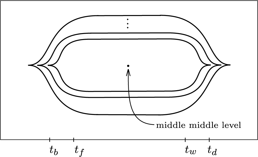
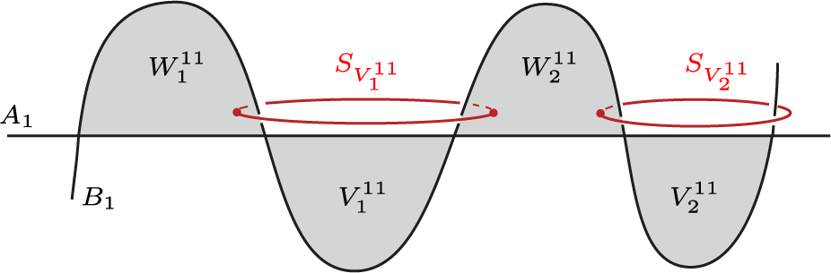


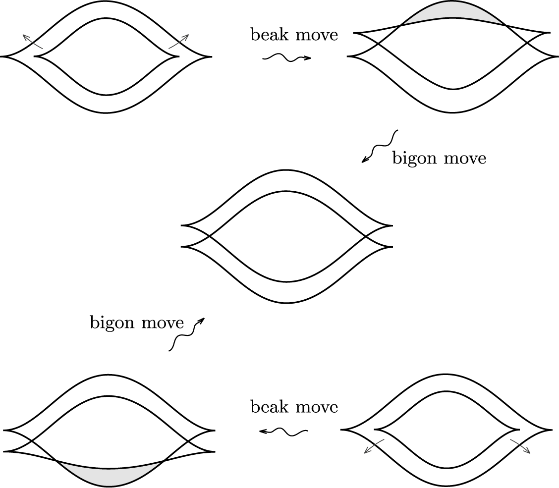


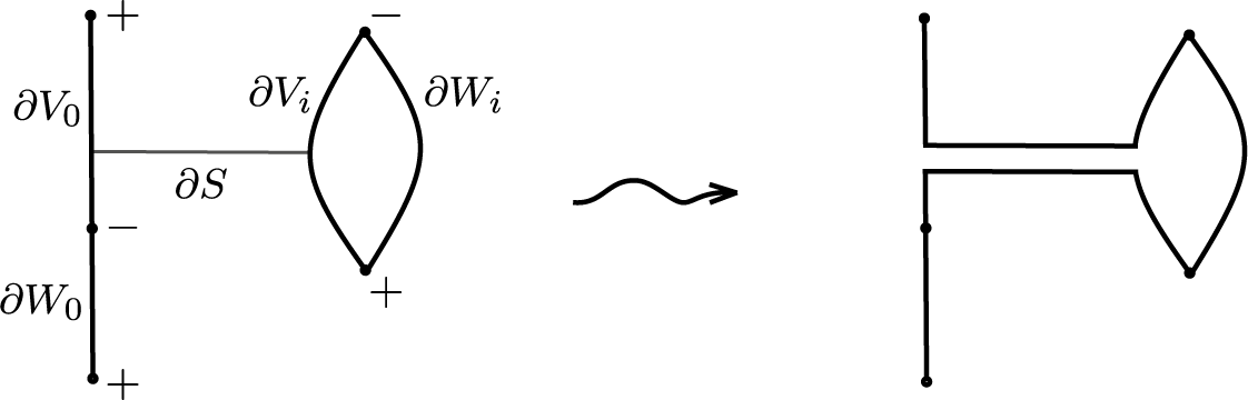


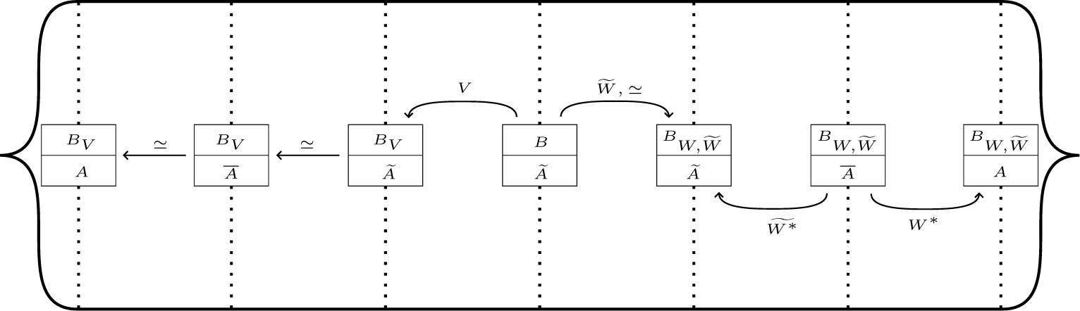


 Open access