


Introduction
Aeolian sediments in the North American midcontinent provide an important terrestrial archive of Late Pleistocene and Holocene paleoenvironmental conditions (Muhs and Zárate, Reference Muhs, Zárate and Markgraf2001). Loess and aeolian sand are widespread along the southern margin of the Laurentide Ice Sheet (LIS) and have a rich history of investigation (e.g., Thorp and Smith, Reference Thorp and Smith1952; Fehrenbacher et al., Reference Fehrenbacher, White, Ulrich and Odell1965; Ruhe and Olson, Reference Ruhe and Olson1980; Mason et al., Reference Mason, Nater and Hobbs1994, Reference Mason, Joeckel and Bettis2007; Jacobs et al., Reference Jacobs, Knox and Mason1997; Bettis et al., Reference Bettis, Muhs, Roberts and Wintle2003; Miao et al., Reference Miao, Hanson, Wang and Young2010; Wang et al., Reference Wang, Stumpf, Miao and Lowell2012; Schaetzl and Attig, Reference Schaetzl and Attig2013; Schaetzl et al., Reference Schaetzl, Running, Larson, Rittenour, Yansa and Faulkner2022; Grimley et al., Reference Grimley, Loope, Jacobs, Nash, Dendy, Conroy and Curry2024). Near the Marine Oxygen Isotope Stage (MIS) 2 (Wisconsin glaciation) maximum limit of the Lake Michigan Lobe and Huron-Erie Lobe in the southern Great Lakes region, studies of loess stratigraphy (McKay, Reference McKay1979), chronology of deposition (Forman et al., Reference Forman, Bettis, Kemmis and Miller1992; Nash et al., Reference Nash, Conroy, Grimley, Guenthner and Curry2018; Grimley et al., Reference Grimley, Loope, Jacobs, Nash, Dendy, Conroy and Curry2024), and provenance through geochemistry, mineralogy, thickness, and particle size (Olson and Ruhe, Reference Olson and Ruhe1979; Grimley, Reference Grimley2000; Muhs et al., Reference Muhs, Bettis and Skipp2018; Dendy et al., Reference Dendy, Guenthner, Grimley, Conroy and Counts2021; Curry, Reference Curry2024) have improved the understanding of connections between loess deposition and paleoclimate, paleo-vegetation, and fluctuations of the southern margin of the LIS. Studies of aeolian sand (non-coastal) in the southern Great Lakes region documenting Late Pleistocene and Holocene dune activity (Miao et al., Reference Miao, Hanson, Wang and Young2010; Campbell et al., Reference Campbell, Fisher and Goble2011; Kilibarda and Blockland, Reference Kilibarda and Blockland2011; Wang et al., Reference Wang, Stumpf, Miao and Lowell2012; Fisher et al., Reference Fisher, Horton, Lepper and Loope2018; Miao, Reference Miao2024) have provided important insight into the control of sediment supply (mainly governed by glacial processes), sediment availability (mainly controlled by surface conditions linked to vegetation), and transport capacity on dune activity (Kocurek and Lancaster, Reference Kocurek and Lancaster1999). Near the MIS 2 maximum limit of the Huron-Erie Lobe in south-central and west-central Indiana, dunes and sand sheets adjacent to former meltwater pathways in the East Fork White River, West Fork White River, and Wabash River valleys (Figs. 1 and 2) provide an opportunity to establish minimum-limiting ages for outwash aggradation and constrain the timing of LIS advance into and retreat out of the White River and Wabash River basins. Parabolic dunes also provide additional paleoenvironmental information, including paleowind direction (Conroy et al., Reference Conroy, Karamperidou, Grimley and Guenthner2019) and surface conditions linked to vegetation cover (e.g., Dijkmans and Koster, Reference Dijkmans and Koster1990).
(A) Maximum extent of North American glacial ice during Marine Oxygen Isotope Stage (MIS) 2 (Ehlers et al., Reference Ehlers, Gibbard, Hughes, Ehlers, Gibbard and Hughes2011; Dalton et al., Reference Dalton, Dulfer, Margold, Heyman, Clague, Froese and Gauthier2023). Red box denotes area in B, which includes the Lake Michigan Lobe (M) and Huron-Erie Lobe (H-E) of the Laurentide Ice Sheet. (B) Hillshade digital elevation model covering the southern Great Lakes region with the MIS 2 maximum limit (black line) and recessional moraines of the Lake Michigan Lobe and Huron-Erie Lobe (dark gray; Illinois: Willman and Frye [Reference Willman and Frye1970]; Indiana: modified from Wayne [Reference Wayne1958, Reference Wayne1965] and this study; Ohio: Pavey et al. [Reference Pavey, Goldthwait, Brockman, Hull, Swinford and Van Horn1999]). The spatial extent of outwash (orange) and aeolian sand (yellow) is from the USDA-NRCS STATSGO2 database (Soil Survey Staff, 2025). Solid white line denotes the modern drainage basin of the White River, a tributary of the Wabash River.

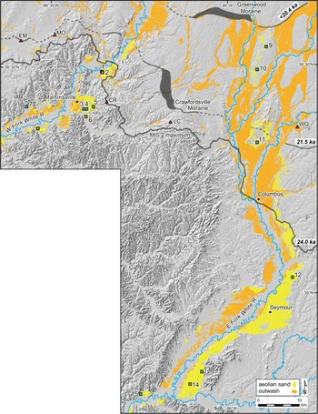
Hillshade digital elevation model of the study area, showing the Marine Oxygen Isotope Stage (MIS) 2 maximum limit (dark gray solid line), recessional moraines (Crawfordsville Moraine: Wayne [Reference Wayne1965]; Greenwood Moraine), the spatial extent of outwash (orange) and aeolian sand (yellow) from the USDA-NRCS SSURGO database (Soil Survey Staff, 2025), sites of this study (numbered green squares), and sites constraining Laurentide Ice Sheet advance and retreat (red triangles, Figure 8; EM = Lake Eminence site; MO = Monrovia site; CR = Centennial Road site; LC = Lick Creek site; WQ = Ward Quarry site; Loope et al., Reference Loope, Antinao, Monaghan, Autio, Curry, Grimley, Huot, Lowell, Nash and Florea2018; Grimley et al., Reference Grimley, Loope, Jacobs, Nash, Dendy, Conroy and Curry2024). Numbers next to moraines denote age (cal ka BP) of ice margin position (Heath et al., Reference Heath, Loope, Curry and Lowell2018; Loope et al., Reference Loope, Antinao, Monaghan, Autio, Curry, Grimley, Huot, Lowell, Nash and Florea2018).

The objective of this study is to determine the timing of deposition of aeolian sand, glaciofluvial sand (outwash), and slackwater sediments using optically stimulated luminescence (OSL) and radiocarbon dating in the White River drainage basin in south-central Indiana in order to investigate the influence of LIS fluctuations, paleoclimate, and paleo-vegetation on the aeolian system.
Study area and geological setting
The study area straddles the MIS 2 maximum limit of the East White Sublobe (Huron-Erie Lobe) of the LIS (Loope et al., Reference Loope, Antinao, Monaghan, Autio, Curry, Grimley, Huot, Lowell, Nash and Florea2018; Figs. 1 and 2). In south-central Indiana, aeolian sand is found adjacent to major meltwater pathways draining the Huron-Erie Lobe of the LIS (Figs. 1 and 2). Gray (Reference Gray1972) and Gray et al. (Reference Gray, Wayne and Wier1970, Reference Gray1972, Reference Gray, Bleuer, Hill and Lineback1979) identified valley train outwash and aeolian sand in the East Fork and West Fork White River valleys as a part of 1:250,000-scale geologic mapping across south-central Indiana. Larger-scale soil mapping completed by the USDA SCS/NRCS (Soil Survey Geographic Database [SSURGO]; Soil Survey Staff, 2025) supplements smaller-scale geologic mapping in identifying aeolian sand deposits. Dunes and sand sheets are located along the eastern edges of the East Fork and West Fork White River valleys, with minor occurrences along the western edges, as a result of dominantly westerly winds during and after the last glacial maximum (Conroy et al., Reference Conroy, Karamperidou, Grimley and Guenthner2019). Detailed investigation of aeolian sand in the White River drainage basin has been limited. Miles and Franzmeier (Reference Miles and Franzmeier1981) studied soils formed in aeolian sand near the southern end of the West Fork White River drainage basin as part of a wider investigation regarding the degree of soil development in dunes from Late Pleistocene to Late Holocene in age across Indiana. Frasier and Gray (Reference Frasier and Gray1992) report on the Late Pleistocene and Holocene history of the West Fork White River and a tributary, Prairie Creek, in southwestern Indiana. Aeolian sand is highlighted in cross sections and maps, but no detailed investigation of the sediments other than particle size was completed.
Apart from valley train outwash and aeolian sand in the East Fork White River and West Fork White River valleys (Fig. 2), the surficial geology in areas north of the MIS 2 maximum limit is dominated by till (Trafalgar Fm.; Wayne, Reference Wayne1963; Gray et al., Reference Gray, Bleuer, Hill and Lineback1979). Three moraines (Crawfordsville Moraine [Wayne, Reference Wayne1965]; Greenwood Moraine; Union City Moraine) record northward recession of the East White Sublobe after the local last glacial maximum (Figs. 1 and 2). The chronology of MIS 2 advance and retreat within the White River drainage basin (∼27 to 19 cal ka BP) is constrained by maximum-limiting radiocarbon ages on organic material within or below till in the study area (sites denoted with red triangles in Fig. 2: sites EM [Lake Eminence], MO [Monrovia], CR [Centennial Road], LC [Lick Creek], and WQ [Ward Quarry]; Heath et al., Reference Heath, Loope, Curry and Lowell2018; Loope et al., Reference Loope, Antinao, Monaghan, Autio, Curry, Grimley, Huot, Lowell, Nash and Florea2018; Grimley et al., Reference Grimley, Loope, Jacobs, Nash, Dendy, Conroy and Curry2024) and minimum-limiting radiocarbon ages on basal organic material from wetlands in east-central Indiana (Glover et al., Reference Glover, Lowell, Wiles, Pair, Applegate and Hajdas2011; Heath et al., Reference Heath, Loope, Curry and Lowell2018). Maximum-limiting radiocarbon ages from three sites within 5 km of the local last glacial maximum limit (sites MO, CR, and LC; Loope et al., Reference Loope, Antinao, Monaghan, Autio, Curry, Grimley, Huot, Lowell, Nash and Florea2018; Fig. 2) indicate the East White Sublobe reached its maximum limit around 24.0 cal ka BP. Subsequent retreat and readvance to the Crawfordsville Moraine at 21.5 cal ka BP is recorded at two sites (EM and WQ; Loope et al., Reference Loope, Antinao, Monaghan, Autio, Curry, Grimley, Huot, Lowell, Nash and Florea2018; Grimley et al., Reference Grimley, Loope, Jacobs, Nash, Dendy, Conroy and Curry2024; Fig. 2). Additional retreat and standstill of the ice margin formed the Greenwood Moraine shortly after 20.4 cal ka BP based on minimum-limiting radiocarbon ages on gastropods within loess south of the moraine (site 10 from this study; Fig. 2). The timing of further northeastward retreat is constrained by minimum-limiting basal radiocarbon ages from wetlands that bracket the age of the Union City Moraine between 19.6 and 18.7 cal ka BP (Glover et al., Reference Glover, Lowell, Wiles, Pair, Applegate and Hajdas2011).
The landscape south of the MIS 2 maximum limit is dominated by Mississippian bedrock (Borden Gp. siliciclastics and Sanders Gp. carbonates) near the surface and MIS 6 (Illinoian glaciation) glacial sediments outside the East Fork and West Fork White River valleys. Within the valleys, MIS 2 slackwater sediments are found adjacent to valley train deposits (Figs. 3 and 4). This is especially noteworthy in the West Fork White River valley, where terraces composed of fine-grained slackwater sediments are found in low-lying areas at the margins of the valley and in a tributary valley (Indian Creek valley) (Figs. 3 and 4). Thin (<1.5 m) MIS 2 Peoria Loess is present on stable landscape positions outside the MIS 2 maximum limit.
(A) Surficial geologic map of the Martinsville, IN, area (modified from Loope, Reference Loope2016), with study sites 3–6 denoted. (B) Cross section showing the transition between Marine Oxygen Isotope Stage (MIS) 2 valley train outwash deposits of the West Fork White River valley and upland MIS 6 glaciolacustrine sediments. Note the aeolian sand ramp sourced from MIS 2 outwash that climbs >50 m in elevation and traverses >2 km on to the uplands along the east edge of the valley. (C) Cross section containing sites 3 and 4 (and additional borings where no ages were completed), with projection of the deep boring at site 6 (Figure 4) onto the cross section. Optically stimulated luminescence (OSL) ages (ka ± 1σ; Table 1) and associated lab numbers are in plain font. Calibrated radiocarbon ages (median cal ka BP; Table 2) are denoted with bold font. (D) Cross section of site 5 (traversing a dune crest) showing interbedded aeolian sand and loess, OSL ages (ka ± 1σ; Table 1), and samples collected for clay mineralogy (Supplementary Figure S7).

(A) Hillshade digital elevation model of the West Fork White River valley and adjacent uplands near Martinsville, IN. Denoted are the Marine Oxygen Isotope Stage (MIS) 2 maximum limit (dark gray solid line), the Crawfordsville Moraine (dark gray dashed and solid line; Wayne, Reference Wayne1965; Figure 2), the spatial extent of outwash (orange), aeolian sand (yellow), and slackwater sediment (blue) inferred from the USDA-NRCS SSURGO database (Soil Survey Staff, 2025), sites 1–8 of this study (numbered green squares), and sites constraining Laurentide Ice Sheet advance and retreat (red triangles, Figure 8; EM = Lake Eminence site, MO = Monrovia site, CR = Centennial Road site; Loope et al., Reference Loope, Antinao, Monaghan, Autio, Curry, Grimley, Huot, Lowell, Nash and Florea2018). Numbers next to moraines denote age (cal ka BP) of ice margin position (Heath et al., Reference Heath, Loope, Curry and Lowell2018; Loope et al., Reference Loope, Antinao, Monaghan, Autio, Curry, Grimley, Huot, Lowell, Nash and Florea2018). (B) Stratigraphy, particle size (volume %), and calibrated radiocarbon ages (cal ka BP; Table 2) for site 6, which records slackwater aggradation in the Indian Creek valley immediately adjacent to the West Fork White River valley (Figure 3). Calibrated radiocarbon age (21.0 cal ka BP) at the top of the core represents the extrapolated age to the surface based on a Bayesian age–depth model (Bacon; Blaauw and Christen, Reference Blaauw and Christen2011; data not shown). Italics for calibrated radiocarbon ages denote ages not included in an age–depth model as determined by Bacon. Modified from Loope et al. (Reference Loope, Antinao, Monaghan, Autio, Curry, Grimley, Huot, Lowell, Nash and Florea2018). (C) Stratigraphy, particle size (volume %), calibrated radiocarbon age (cal ka BP; Table 2), and optically stimulated luminescence (OSL) ages (ka; Table 1, Supplementary Table S2) for site 7. Two cores were collected at site 7, roughly 300 m apart. Italics for OSL sample IGWS-338 (35.3 ± 3.2 ka) indicate the age is not used in reconstruction of the timing of glacial and aeolian events in the study area.

Methods
Soils data from the USDA-NRCS SSURGO database (Soil Survey Staff, 2025) were used with GIS (ESRI ArcGIS Pro 3.3) to map the distribution of soils with outwash and aeolian sand parent material (Fig. 2). The validity of the soils data was corroborated throughout the study area with LIDAR digital elevation models showing aeolian landforms (e.g., dunes) and glaciofluvial landforms (e.g., braid bars). Sites for OSL and radiocarbon dating were selected to capture the broad spatial distribution of aeolian sand and outwash in both the East Fork and West Fork White River basins. The selection of sites to determine the chronology of aeolian sand activity focused on capturing a variety of aeolian landforms (sand sheets/ramps [sites 4, 5]; simple, isolated parabolic dunes [sites 9–11]; large, compound parabolic dunes [sites 12–14]) over a broad spatial extent in both the East Fork and West Fork White River basins. Site selection for determining the chronology of outwash/slackwater aggradation focused on the West Fork White River valley, as prior mapping (Loope, Reference Loope2016) identified valley train outwash terraces and slackwater terraces suitable for additional investigation.
Samples for OSL dating were collected from cores taken with direct-push techniques (3.2 to 7.6 cm diameter; sites 1–4, 7, 8), from bucket augering (sites 5, 9–15), and directly from outcrop (site 13). At sites 1–4 and 7, an initial core was collected to determine the stratigraphy and best interval(s) for luminescence sampling. A second core was collected adjacent to the first with opaque liners at selected depth interval(s). OSL samples were taken from a ca. 15 cm interval from the core segments collected with opaque liners (e.g., Supplementary Fig. S2A). At site 8, a 7.6-cm-diameter core was collected, and OSL samples were collected in 4.8-cm-diameter stainless steel cylinders pushed directly into the bottom segment of the core in the field. At sites 5 and 9–15, an 8.3-cm-diameter sand bucket auger was used initially to determine the stratigraphy and collect samples for particle size analysis and water content. A second, adjacent hole was used to collect OSL samples from selected depths. Once the selected depth was reached with the auger, a 4.8 cm (D) × 15.2 cm (L) stainless steel cylinder was pushed into the top of the bucket, then removed, capped, and labeled. At site 13, an exposure of aeolian sand was sampled directly from cleaned, vertical faces with 4.8 cm (D) × 15.2 cm (L) stainless steel cylinders. Additionally, a bucket auger was used to collect OSL samples from a greater depth at the site, from the floor of the sand pit. All OSL samples were collected from depths ≥2 m from the surface within the C horizon in order to minimize the influence of pedoturbation and/or pedogenesis (Hanson et al., Reference Hanson, Mason, Jacobs and Young2015; Table 1).
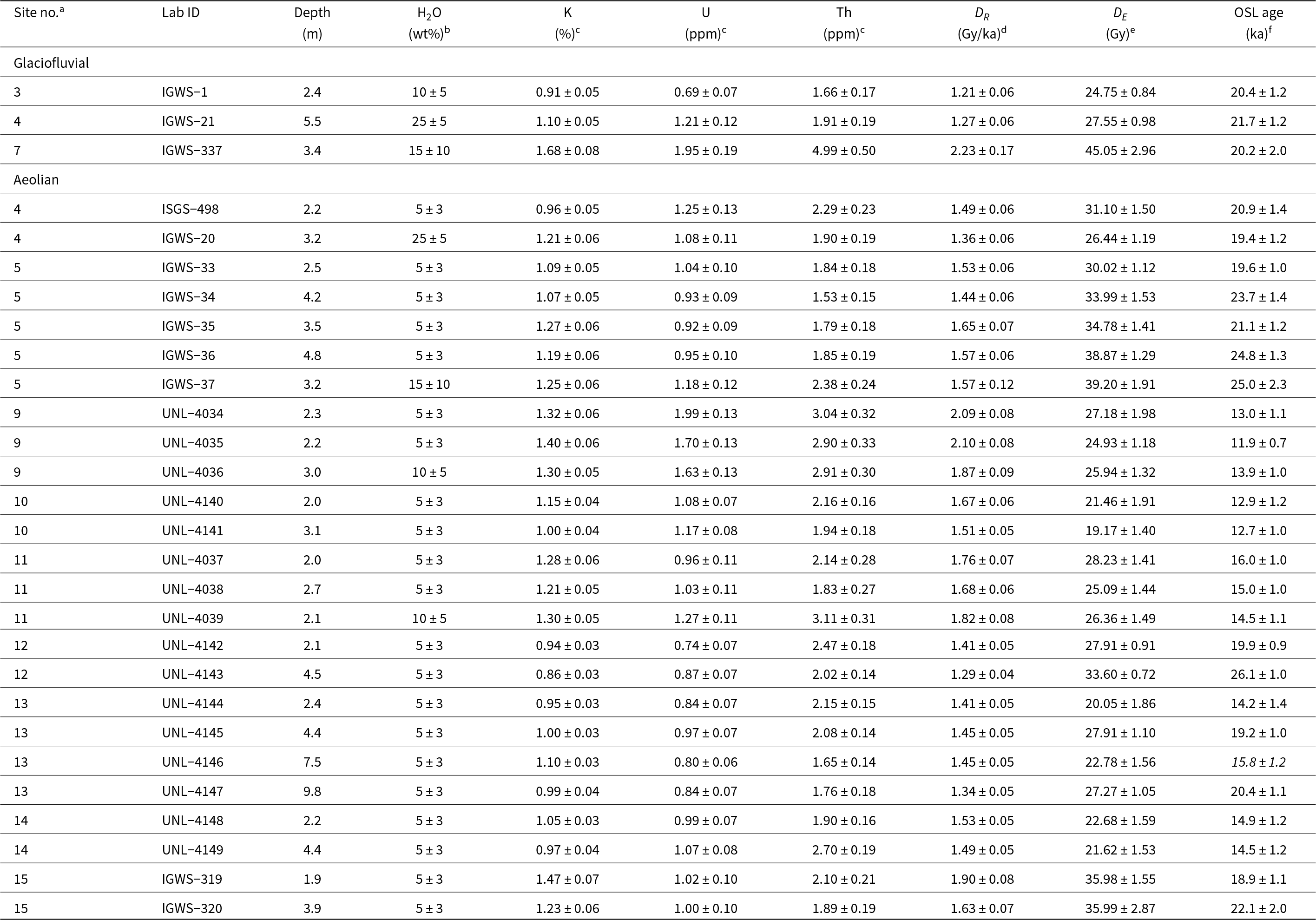
Optically stimulated luminescence (OSL) ages and associated data for glaciofluvial and aeolian quartz sand from the White River drainage basin, south-central Indiana.

a Site locations are found in Figure 2 and Supplementary Table S3. Data on additional glaciofluvial samples from sites 1, 2, 7, and 8 are found in Supplementary Table S2.
b Long-term water content estimated from gravimetric methods and soil water content modeling results based on particle size (methodology from Nelson and Rittenour, Reference Nelson and Rittenour2015). See Supplementary Figs. S2C and S4 for additional data.
c ± 1 standard deviation; elemental analysis was determined by high-resolution gamma spectrometry (UNL and ISGS laboratory IDs) and by inductively coupled plasma–mass spectrometry (ICP–MS) and inductively coupled plasma–atomic emission spectrometry (ICP–AES) (IGWS laboratory IDs). Value represents the average of two or more samples collected for elemental analysis.
d Total environmental dose rate (DR); ± 1 standard deviation; calculated using the Dose Rate and Age Calculator (DRAC) (Durcan et al., Reference Durcan, King and Duller2015); see Supplementary Material Table S4 for additional data.
e Equivalent dose (DE); ± 1 standard error; calculated using the central age model (CAM) (Galbraith et al., Reference Galbraith, Roberts, Laslett, Yoshida and Olley1999); see Supplementary Material Figures S2, S5, and S6 for additional data.
f ± 1 standard deviation; kiloyears before 2016 for UNL and ISGS laboratory IDs and kiloyears before 2024 for IGWS laboratory IDs; italics denote age was not used in regional assessment of aeolian chronology (site 13; UNL-4146); age and equivalent doses of UNL laboratory ID samples have been adjusted upward 8.25% to account for adjustments to the Risø calibration quartz standard (Autzen et al., Reference Autzen, Andersen, Bailey and Murray2022).
Samples were processed at three different laboratories—the Landscape Evolution and Luminescence Geochronology Laboratory at the University of Nebraska–Lincoln (UNL lab IDs; Table 1), the Luminescence Geochronology Laboratory at the Illinois State Geological Survey, University of Illinois Urbana–Champaign (ISGS lab IDs; Table 1), and the Luminescence Geochronology Laboratory at the Indiana Geological and Water Survey, Indiana University (IGWS lab IDs; Table 1). Cores with opaque liners and samples collected with 4.8 cm (D) × 15.2 cm (L) stainless steel cylinders were opened in darkroom conditions. Cores were split and sampled directly from a ca. 15 cm core segment. In addition to the OSL sample, multiple samples were taken for elemental analysis and water content within 30 cm of the OSL sample for dose rate determination. For OSL samples collected with stainless steel cylinders, the outer 5 cm of sediment was removed from the ends of the tube, which were subsequently analyzed for elemental concentrations. Elemental concentrations (U, Th, K, Rb) for calculation of the dose rate were determined by high-resolution gamma spectrometry, inductively coupled plasma–mass spectrometry (ICP–MS), and inductively coupled plasma–atomic emission spectrometry (ICP–AES). High-resolution gamma spectrometry was used for samples analyzed at the University of Nebraska–Lincoln (UNL lab IDs) and the Illinois State Geological Survey (ISGS lab IDs). Samples from the Indiana Geological and Water Survey (IGWS lab IDs) were analyzed by ICP–MS and ICP–AES following a lithium borate fusion (ME-MS81d) at ALS Laboratories (Reno, NV). Gravimetric water content was measured by weight loss upon drying at 100°C for >48 hours. In addition to samples for water content being collected within 30 cm of the OSL sample (those from cores and outcrop), gravimetric water content (weight %) was determined every 20 cm downhole at four sites (sites 4, 10, 12, and 14; Supplementary Figs. S2C and S4). A representative value of 5 ± 3% was used for samples within the vadose zone (21 out of 28 OSL samples; Table 1) based on the downhole water content data, modeled water content using particle size (methods in Nelson and Rittenour [Reference Nelson and Rittenour2015]; Supplementary Figs. S2C and S4), and comparisons to prior work on water content in dune sand in temperate climates (e.g., Gardner and McLaren, Reference Gardner and McLaren1999). Higher water content values (10%, 15%, 25%) for the remaining seven samples were based on presence within the modern capillary fringe (10%, 15%) or saturated zone (25%). OSL samples were wet sieved to isolate the 90–150, 150–250, or 180–250 µm fraction, then treated with 1 N hydrochloric acid (HCl) to remove carbonates. Samples collected for this study had very little or no organic material, so treatment with hydrogen peroxide (H2O2) was not completed. Quartz and K-feldspar were separated from the heavy mineral fraction by flotation in sodium polytungstate (UNL lab IDs), lithium metatungstate (IGWS IDs), or lithium heteropolytungstate (ISGS lab ID). Quartz grains were etched and feldspars were removed by a hydrofluoric acid (HF) (48%) treatment for 60–70 minutes. A second HCl treatment was given to remove calcium fluoride minerals produced during HF dissolution. Samples were re-sieved to a final fraction for OSL analysis (90–150, 150–250, or 180–250 µm). Quartz grains were mounted on aluminum or stainless steel disks with a ca. 5 mm mask (hundreds of grains per disk) for aeolian samples and a ca. 1 mm mask (tens of grains per disk) for glaciofluvial samples using silicon oil. OSL measurements were performed on a Risø TL/OSL-DA-20 (UNL lab IDs) and a Freiberg Lexsyg Smart reader (IGWS and ISGS lab IDs), using blue light (470 and 458 nm; UNL and IGWS lab IDs) or green light (525 nm; ISGS lab ID) stimulation. Optical measurements were made at 125°C. Infrared (870 and 850 nm) stimulation was used to check for feldspar contamination. Equivalent doses (DE) were determined using the single-aliquot regenerative (SAR) protocol (Murray and Wintle, Reference Murray and Wintle2000, Reference Murray and Wintle2003). Results from dose recovery and preheat plateau tests on select samples indicated the validity of the SAR protocol for samples from the study area (Supplementary Fig. S5). A 200°C, 10 second preheat was used for the natural and regenerative measurements, and a 180°C, 0 second preheat (cutheat) was used for test dose measurements. Four or five regenerative doses were used to bracket the natural signal, with the final dose being a repeat of the first regenerative dose. Test doses (∼3–5 Gy) were applied after measurement of the natural and regenerative signals to monitor changes in sensitivity. The Analyst software package (v. 4.56) (Duller, Reference Duller2015) was used to view OSL data (IGWS lab IDs) and accept or reject aliquots based on several criteria, including the recycling ratio (within ±10%), test dose error (<10%), and recuperation (<5%). Aliquots were also rejected if anomalous shinedown curves indicated contribution from non-quartz (feldspar) sources or medium/slow components of the OSL signal. Growth curves were fit with saturating exponential or saturating exponential with linear component equations to estimate the equivalent dose. Equivalent doses were adjusted upward by 8.25% from the original measured values for samples analyzed at University of Nebraska–Lincoln (UNL lab IDs) to adjust for corrections in Risø calibration quartz (Autzen et al., Reference Autzen, Andersen, Bailey and Murray2022). The R package Luminescence was used to view and plot equivalent dose data (Kreutzer et al., Reference Kreutzer, Burow, Dietze, Fuchs, Schmidt, Fischer and Friedrich2024). The central age model (Galbraith et al., Reference Galbraith, Roberts, Laslett, Yoshida and Olley1999) was used for DE determination and the dose rate (DR) was calculated using the Dose Rate and Age Calculator (DRAC; Durcan et al., Reference Durcan, King and Duller2015). Ages are reported as thousands of years (ka) before 2016 (UNL and ISGS lab IDs) or 2024 (IGWS IDs). Additional OSL data are included in the Supplementary Material (Supplementary Figs. S1–S6, Supplementary Tables S1 and S2).
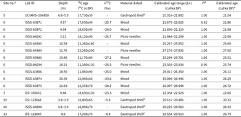
Samples for radiocarbon dating were taken directly from cores (sites 6, 7) and from bucket auger samples (sites 5, 10, and 13). Organic samples (sites 6, 7) were sieved and cleaned with distilled water and dried at 60°C for >48 hours. Identifiable wood fragments and Picea needles were selected for accelerator mass spectrometry (AMS) radiocarbon dating (Table 2). Gastropod shells from sites 5, 10, and 13 (Figs. 3, 5, and 6, Table 2) were selected for AMS radiocarbon dating. Shells were encountered during bucket augering and were found within silt (loess) beds, which are interbedded with aeolian sand at several sites. Gastropod shell identification and cleaning followed the procedures in Grimley et al. (Reference Grimley, Loope, Jacobs, Nash, Dendy, Conroy and Curry2024). Eleven samples were sent to the Illinois State Geological Survey Radiocarbon Dating Laboratory (ISGS lab code; Table 2) for pretreatment with subsequent AMS measurements completed at the W. M. Keck Carbon Cycle Accelerator Mass Spectrometer Facility (University of California–Irvine; UCIAMS lab code). Three samples were sent to the National Ocean Sciences Accelerator Mass Spectrometry Facility (Woods Hole Oceanographic Institution; OS lab code; Table 2) for pretreatment and AMS measurements. One sample was sent to the W. M. Keck Carbon Cycle Accelerator Mass Spectrometer Facility (University of California–Irvine; UCIAMS lab code; Table 2) for pretreatment and AMS measurement. Radiocarbon ages were calibrated with CALIB rev. 8 (Stuiver and Reimer, Reference Stuiver and Reimer1993) using the IntCal20 calibration curve (Reimer et al., Reference Reimer, Austin, Bard, Bayliss, Blackwell, Bronk Ramsey and Butzin2020). Ages are reported as the median cal ka BP (Table 2).
Radiocarbon ages and associated data.

a Site locations are found in Fig. 2.
b Succineidae.
c Stagnicola elodes.
d Probability (P) of age being within 2σ calibrated age range. Probabilities below 0.10 (10%) are not shown.
e Median calibrated age rounded to the nearest 10 yr. Calibrated with CALIB 8.20 (Stuiver and Reimer, Reference Stuiver and Reimer1993) using the IntCal20 calibration curve (Reimer et al., Reference Reimer, Austin, Bard, Bayliss, Blackwell, Bronk Ramsey and Butzin2020).
Samples for particle size analysis were collected directly from cores or from bucket auger samples and were subsequently air-dried and gently crushed with a mortar and pestle. Samples were sieved to <2 mm and <1.4 mm if gravel or very coarse sand was present (select samples from sites 1, 2, and 8). Samples with a maximum grain size of >1.4 mm were sieved at 0.5 or 1 phi (ɸ) intervals (ɸ = log2 D, where D = particle diameter in mm), from −5 to −0.5 phi (32 mm to 1.4 mm), using a sieve shaker. The mass of the >1.4 mm fraction(s) was recorded. The particle size distribution for samples with a maximum grain size of <1.4 mm (most samples) and the <1.4 mm fraction from coarser sediment samples was determined using laser diffraction on a Malvern Mastersizer 3000. Samples were dispersed with a 5 g/L solution of sodium metaphosphate and subject to 120 seconds of 40 W in-line sonication before measurement. Samples were run in triplicate using a Hydro EV wet dispersion unit for 40 seconds each with a stirrer speed of 3000 revolutions per minute. These three runs were averaged for a final result. Mie scattering with a particle refractive index of 1.544, a particle absorption index of 1.0, and a dispersant refractive index of 1.33 (water) were used to determine the final grain size distribution. Results from laser diffraction analysis are reported in volume percent. For those samples with particles >1.4 mm, the mass percent for each fraction was added (“extended”) on to the volume percent for the <1.4 mm fraction, completed using Mastersizer software v. 3.86. The mixing of mass- and volume-based measurements is problematic, although few options exist for displaying both the finer and coarser fractions together (e.g., as gravel, sand, silt, and clay percentages). In this study, this issue is somewhat diminished, in that our interpretations are based on relative particle size changes and/or the presence (or absence) of certain particle sizes (gravel, for example). An additional complication is the underestimation of the clay (<2 µm) fraction by laser diffraction relative to sedimentation (pipette) techniques (Konert and Vandenberghe, Reference Konert and Vandenberghe1997; Beuselinck et al., Reference Beuselinck, Govers, Poesen, Degraer and Froyen1998). In this study, we used 4 µm as the clay–silt boundary, based on replicate analysis of 119 samples from a variety of Quaternary sediments in Indiana by both laser diffraction and pipette techniques (data not shown). In plots of particle size in this paper, we present volume percent of clay (<4 µm), silt (4–63 µm), sand (63–2000 µm), and gravel (>2000 µm).
Ground penetrating radar (GPR) data were collected at site 13 (Figs. 2, 6, and 7) along an east–west 60-m-long transect on the floor of the borrow pit using a 250 MHz Sensors and Software Noggin SmartCart to investigate aeolian sand stratification and deeper stratigraphy at the site. Data were collected in common-offset mode with traces collected at 5 cm intervals (stack = 8). The LineView module in Sensors and Software EKKO Project (v. 5) software was used to create a topographically corrected cross section. GPR data were displayed after using a Dewow filter and automatic gain control amplification with migration. A velocity of 0.15 m/ns was used to calculate depths.
Samples for clay mineralogy were collected from bucket auger samples of silt beds found interbedded with aeolian sand at sites 5, 10, 11, 12, and 15. Samples were analyzed to determine provenance of the silt and possible correlation with Peoria Silt (loess). The samples were air-dried, gently crushed with a mortar and pestle, and added to a 5% solution of sodium metaphosphate and shaken overnight. Clay (<2 µm) was subsequently separated by sedimentation and was sampled by pipette (after 3 hours, 51 minutes at 5 cm depth [21°C]). Individual samples were Mg-saturated, smeared onto glass slides, and ethylene glycol solvated before analysis by X-ray diffraction. X-ray diffraction analysis was completed with a Rigaku Miniflex X-Ray diffractometer using Cu-kα radiation with a scan speed of 2° per minute and a step size of 0.02°. Slides were scanned from 3 to 31.5° two-theta. JADE software was used to analyze peak heights and identify clay minerals.
Results
Aeolian sand distribution
Aeolian sand is found within and along the eastern margin of the West Fork and East Fork White River valleys (Fig. 2). These valleys were major meltwater pathways sourced from the East White Sublobe of the Huron-Erie Lobe (Schneider and Gray, Reference Schneider and Gray1966), during both advance to the maximum limit and deglaciation from south to north across the basin. Dominantly westerly winds (Conroy et al., Reference Conroy, Karamperidou, Grimley and Guenthner2019) reworked outwash in these valleys and transported aeolian sand eastward up to a distance of 10 km along the eastern flanks of the valleys. In several cases, aeolian sand ramps developed, and aeolian sand is found up to 50 m above the maximum elevation of outwash aggradation (e.g., sites 5, 13; Figs. 3B and 6). South of the MIS 2 maximum limit, aeolian sand is generally thicker (can be >10 m thick) and more extensive (e.g., forms sand sheets) than aeolian sand located north of the MIS 2 maximum limit. North of the maximum limit, aeolian sand is typically thin (<4 m thick) and forms isolated parabolic dunes (sites 9–11; Fig. 5). The stratigraphy and chronology of sites associated with glaciofluvial and slackwater aggradation are presented first, followed by the stratigraphy and chronology of aeolian sand sites.
Spatial extent of outwash (orange) and aeolian sand (yellow) based on USDA-NRCS SSURGO database (Soil Survey Staff, 2025) draped over hillshade digital elevation models, with corresponding stratigraphy, optically stimulated luminescence (OSL) ages (ka; Table 1), and calibrated radiocarbon ages (cal ka BP; Table 2) for sites 9–11. Sampling sites (green squares) are located along the crest of parabolic dune arms and noses. Star symbol indicates clay mineralogy samples collected from thin loess beds within aeolian sand (Supplementary Figure S7).

Glaciofluvial (outwash) and slackwater sediment chronology
The chronology of outwash and slackwater aggradation in the West Fork White River valley and Indian Creek (a tributary valley) is presented in Figures 3 and 4 (sites 6, 7) and Supplementary Figures S1–S3 (sites 1–4, 8). At sites 1 and 2 (Supplementary Fig. S1), OSL ages on glaciofluvial sand (all three samples) range from 42.3 to 27.5 ka (Supplementary Table S2). The minimum age model (MAM; Galbraith et al., Reference Galbraith, Roberts, Laslett, Yoshida and Olley1999) (overdispersion (σ) = 25%; Supplementary Fig. S1) was used, but gave ages interpreted to be too old based on regional glacial chronology (Heath et al., Reference Heath, Loope, Curry and Lowell2018; Loope et al., Reference Loope, Antinao, Monaghan, Autio, Curry, Grimley, Huot, Lowell, Nash and Florea2018) as well as a radiocarbon-dated slackwater succession (site 6) <10 km to the south. At sites 3 and 4 (Fig. 3), two OSL ages on glaciofluvial sand (IGWS-1 and IGWS-21) range between 21.7 and 20.4 ka (Table 1). These samples represent the final stages of outwash aggradation in the West Fork White River valley. The central age model (CAM; Galbraith et al., Reference Galbraith, Roberts, Laslett, Yoshida and Olley1999) was used based on the DE distributions (∼normal distribution; Supplementary Fig. S2). Site 6 records >20 m of slackwater sedimentation in the Indian Creek valley, a tributary to the West Fork White River valley (Figs. 3 and 4). Ten radiocarbon ages constrain deposition between 26.7 and 21.9 cal ka BP (Fig. 4B, Table 2). Based on a Bayesian age–depth model (Bacon; Blaauw and Christen, Reference Blaauw and Christen2011), two radiocarbon ages between 10 m and 12 m depths (ISGS-A4385 and ISGS-A4384) were not considered (in italics in Fig. 4B), as the ages are out of stratigraphic order. The age–depth model was extrapolated to the surface and returned an age of 21.0 cal ka BP. We take this as the age estimate of the end of slackwater aggradation in the Indian Creek valley, which is tied directly to outwash aggradation in the West Fork White River valley (Figs. 3 and 4). At site 7 (Fig. 4C), two OSL ages on glaciofluvial/glaciolacustrine (slackwater) sand (IGWS-337 and IGWS-338) range between 35.2 and 20.2 ka (Table 1, Supplementary Table S2). The CAM was used for IGWS-337, based partly on the DE distribution and partly on the severe underestimation of the MAM age (12.6 ka) (Supplementary Fig. S6). The MAM was used for IGWS-338 (Supplementary Fig. S6), which provided an age of 35.2 ka (Supplementary Table S2). A second core at site 7 (Fig. 4C) encountered organic material (likely Picea wood) near 9.5 m depth and provided an age of 22.6 cal ka BP (Table 2). The core at site 8 (Supplementary Fig. S3) encountered ca. 2 m of aeolian sand over glaciofluvial sand and gravel. Three OSL ages on glaciofluvial sand range between 33.7 and 27.7 ka (Supplementary Table S2). The CAM was used for IGWS-177 and IGWS-178, while the MAM was used for IGWS-179 (Supplementary Fig. S3). These samples represent the final stages of outwash aggradation in the West Fork White River valley, but are too old based on regional glacial chronology (Heath et al., Reference Heath, Loope, Curry and Lowell2018; Loope et al., Reference Loope, Antinao, Monaghan, Autio, Curry, Grimley, Huot, Lowell, Nash and Florea2018) and results from the radiocarbon-dated slackwater succession at site 6 (ca. 10 km to the east-northeast; Fig. 4A).
Aeolian sand chronology
The chronology of aeolian sand deposition adjacent to the West Fork and East Fork White River valleys is presented in Figures 3, 5, and 6 (sites 4, 5, and 9–15). The West Fork White River sites are presented first, followed by those sites adjacent to the East Fork White River and tributaries. For all aeolian sand OSL samples, the CAM was used in the estimate of the DE. The direct-push core at site 4 (Fig. 3C), taken from a dune crest, encountered ca. 5 m of aeolian sand and interbedded silt (loess) over glaciofluvial sand (Supplementary Fig. S2C). Two OSL ages (ISGS-498 and IGWS-20; Table 1) range between 20.9 and 19.4 ka. These ages are out of stratigraphic order, although they overlap at the 95% confidence interval (error on ages reported at ±1σ). At site 5, five OSL samples were collected over three bucket auger sites across the crest of a dune (Fig. 3D). OSL ages range from 25.0 to 19.6 ka (Table 1), with ages falling in stratigraphic order. Supplementary Figure S5 displays a variety of OSL data plots for IGWS-33, the uppermost sample from site 5. Thin (ca. 20- to 30-cm-thick) silt beds, interpreted as loess, were encountered during bucket augering. Gastropod shells (Succineidae) were found between 4.8 m and 5.0 m depths from the bucket auger site at the crest of the dune (Fig. 3D) and returned an age of 21.54 cal ka BP (Table 2). This radiocarbon age is out of stratigraphic order, although it overlaps at the 95% confidence interval with the OSL age above it (IGWS-34) and agrees well with OSL ages (e.g., IGWS-35) from the adjacent bucket auger site. OSL ages, coupled with the presence of loess beds, suggest that the dune built up (aggraded) over several thousand years, related to pulses of aeolian sand migrating upslope over 50 m in elevation from the active valley train outwash surface in the West Fork White River valley (Fig. 3B).
Sites 9–15 are located along the eastern edge of valley train outwash deposits of the East Fork White River and tributaries (Fig. 2). Sites 9–11 are north of the last glacial (MIS 2) maximum limit and contain 3–4 m of aeolian sand and minor interbedded silts over till or silt (loess) (Fig. 5). At sites 9 and 11, two locations (A, B) along the crest of a dune were sampled with a bucket auger. OSL ages from these three sites range from 16.0 to 11.9 ka (Fig. 5, Table 1) and we group them together here based on their similar geomorphic setting and stratigraphy. At site 10, near 4 m depth, a silt (loess) bed containing gastropod shells (Succineidae) was encountered, and two radiocarbon ages (20.32 and 20.41 cal ka BP) were obtained. Sites 12–15 are located south of the last glacial (MIS 2) maximum limit (Fig. 2) and record two phases of aeolian sand activity. An older phase, seen in sites 12, 13, and 15, is represented by six OSL ages ranging from 26.1 to 18.9 ka (Fig. 6, Table 1). A younger phase, seen at sites 13 and 14, is represented by three OSL ages between 15 and 14 ka (Fig. 6, Table 1). At site 13, four OSL samples were collected from an exposure and from bucket auger sampling from the floor of the sand quarry (Figs. 6 and 7). The upper sample (UNL-4144; 14.2 ka) in the exposure was collected within planar cross-bedded aeolian sand, in contrast to the lower sample in the exposure (UNL-4145; 19.2 ka), which was collected within high-angle cross-bedded aeolian sand (Fig. 7A and B). The boundary between the two cross-stratified units represents a ca. 5 ka unconformity, although no evidence of a paleosol or weathering near the contact was present (white line in Fig. 7A and B). The high-angle cross-bedding seen in outcrop (eastward-dipping foresets) continues for an additional 2 m depth below the sand quarry floor based on a GPR profile (Fig. 7C). The OSL age from bucket auger sampling at a composite depth of 7.5 m (UNL-4146; 15.8 ka) is out of stratigraphic order (noted by italic text in Figs. 6 and 7) and is not included in the regional synthesis of ages. A silt bed containing gastropod shells (Stagnicola elodes) was encountered during bucket augering and radiocarbon dating of the shells returned an age of 20.75 cal ka BP (Table 2). The lowermost OSL sample from site 13 provided an age of 20.4 ka, within ±1σ error of the radiocarbon age on a gastropod shell around 1.5 m above it.
Spatial extent of outwash (orange) and aeolian sand (yellow) based on USDA-NRCS SSURGO database (Soil Survey Staff, 2025) draped over hillshade digital elevation models, with corresponding stratigraphy, optically stimulated luminescence (OSL) ages (ka; Table 1), and calibrated radiocarbon ages (cal ka BP; Table 2) for sites 12–15. Sampling sites (green squares) are located along the crest of parabolic dune noses (sites 12–14) and a dune arm (site 15). The outcrop at site 13 (Figure 7) exposes the interior of a parabolic dune nose. The star symbol indicates clay mineralogy samples collected from thin loess beds within aeolian sand (Supplementary Figure S7). Italics for OSL sample UNL-4146 (site 13, 15.8 ± 1.2 ka) indicate the age is out of stratigraphic order and is not used in reconstruction of the timing of aeolian activity in the study area.

(A and B) Photograph of the borrow pit exposure of aeolian sand at site 13 (Vallonia site; Figure 6). View in A is to the west; view in B is to the south. The modern solum is denoted with A and Bt horizons labeled. Black lines denote cross-bedding, and the solid white line denotes an unconformity between two episodes of aeolian sand deposition. No evidence of pedogenesis was found associated with the unconformity. Optically stimulated luminescence (OSL) sample locations are denoted by white squares (Figure 6, Table 1). Location of bucket auger sampling from the floor of the pit is noted in B. (C) Ground penetrating radar (250 MHz) profile across the floor of the borrow pit. The upper panel displays the processed and topographically corrected profile. The lower panel represents the interpretation of the upper panel, with red lines denoting cross-bedding and gray lines denoting bounding surfaces between packages of aeolian sand. Location of bucket auger sampling is denoted, with associated OSL ages (ka; Table 1) and calibrated radiocarbon age (cal ka BP; Table 2).

Clay (<2 µm) mineralogy
Clay (<2 µm) mineralogy data (X-ray diffractograms) from silt (loess) units interbedded with aeolian sand from sites 5, 10, 11, 12, and 15 (Figs. 3, 5, and 6) are highlighted in Supplementary Figure S7. The uppermost diffractogram is from unweathered (C horizon) Peoria Loess from a core near Terre Haute, IN (Terre Haute core in Grimley et al. [Reference Grimley, Loope, Jacobs, Nash, Dendy, Conroy and Curry2024]), located adjacent to the Wabash River. The other diffractograms are grouped by drainage basin. The similarity of the diffractograms between samples from the East Fork White River basin, West Fork White River basin, and the Wabash River basin suggest a similar provenance, corresponding to the regional character of Peoria Loess, which has a significant proportion of smectite relative to illite and kaolinite/chlorite (Jacobs et al., Reference Jacobs, Mason and Hanson2011). In addition, Grimley et al. (Reference Grimley, Loope, Jacobs, Nash, Dendy, Conroy and Curry2024) documented the deposition of Peoria Loess along the Wabash River valley between ca. 28 and <21.9 cal ka BP, which overlaps with the older phase of aeolian sand activity between 26 and 19 ka from the East Fork and West Fork White River valleys.
Discussion
The timing of aeolian sand activity surrounding the local last glacial maximum based on OSL and radiocarbon dating (ca. 26–19 ka) in the West Fork and East Fork White River basins corresponds well with OSL and radiocarbon ages constraining outwash and slackwater aggradation (ca. 27–20 ka) within the West Fork White River basin (Fig. 8B). The chronology of outwash and slackwater aggradation is conceptually linked to the presence of the LIS (East White Sublobe) within the White River drainage basin. Comparison of a time–distance diagram for the East White Sublobe (Fig. 8C) based on minimum- and maximum-limiting radiocarbon ages (Fleming et al., Reference Fleming, Brown and Ferguson1993; Glover et al., Reference Glover, Lowell, Wiles, Pair, Applegate and Hajdas2011; Heath et al., Reference Heath, Loope, Curry and Lowell2018; Loope et al., Reference Loope, Antinao, Monaghan, Autio, Curry, Grimley, Huot, Lowell, Nash and Florea2018; Grimley et al., Reference Grimley, Loope, Jacobs, Nash, Dendy, Conroy and Curry2024) with outwash/slackwater aggradation and aeolian sand activity indicates a strong correlation between the presence of glacial ice in the White River drainage basin (horizontal dashed lines in Fig. 8B and C), outwash/slackwater aggradation, and aeolian sand activity. The oldest maximum-limiting radiocarbon age in the drainage basin (25.7 cal ka BP) comes from Fleming et al. (Reference Fleming, Brown and Ferguson1993), from a Picea log within basal MIS 2 till immediately above the Sangamon Geosol, at a site northeast of Indianapolis. This site is located about 75 km southwest of the modern drainage divide (Fig. 8A) and provides a conservative estimate (age is likely older) for initial MIS 2 advance into the paleo-White River drainage basin (lower horizontal dashed line in Fig. 8B and C). This age is in general agreement with the onset of slackwater aggradation at site 6, just after 27 ka (vertical solid black line in Fig. 8B). The youngest minimum-limiting radiocarbon ages in the drainage basin (or immediately adjacent to the basin) come from Glover et al. (Reference Glover, Lowell, Wiles, Pair, Applegate and Hajdas2011) and indicate the ice margin retreated from the Union City Moraine ca. 19.3 ka and the Mississinewa Moraine ca. 18.7 ka (Fig. 8A and C). The modern White River drainage basin divide is located between the Union City and Mississinewa Moraines (Fig. 8A), suggesting sediment and meltwater flow down the West Fork White River ended ca. 19 ka (upper dashed horizonal line in Fig. 8B and C).
(A) Map of Indiana and adjacent states showing the Marine Oxygen Isotope Stage (MIS) 2 maximum limit (black line); recessional moraines (dark gray); extent of outwash (orange); extent of aeolian sand (yellow); maximum- and minimum-limiting calibrated radiocarbon ages (cal ka BP; red triangles) constraining the advance and retreat of the Laurentide Ice Sheet (LIS); and the modern White River drainage basin (dashed black line). Solid red line denotes the line of the time–distance diagram found in C. (B) Optically stimulated luminescence (OSL) ages (black squares; ±1σ error; Table 1) on aeolian sand and glaciofluvial sediments with calibrated radiocarbon age range (solid vertical black line) of slackwater sedimentation adjacent to the West Fork White River from site 6 (Figure 4), grouped by sub-drainage basin (East Fork and West Fork White River). Dashed black vertical line denotes age extrapolation (to 21.0 ka) to the top of the core at site 6 (Figure 4). C) Time–distance diagram for the Huron-Erie Lobe of the LIS (simplified from Heath et al., Reference Heath, Loope, Curry and Lowell2018), with red triangles denoting maximum- or minimum-limiting constraints on glacial ice cover. Solid red line in A denotes the line of the time–distance diagram. Moraine names are indicated at top of panel (also in A). Dashed black horizontal lines bracket the interval of time (∼27 to ∼19 ka) when the LIS was within the paleo–White River drainage basin. Constraining ages for the time–distance diagram are from Fleming et al. (Reference Fleming, Brown and Ferguson1993), Glover et al. (Reference Glover, Lowell, Wiles, Pair, Applegate and Hajdas2011), Heath et al. (Reference Heath, Loope, Curry and Lowell2018), Loope et al. (Reference Loope, Antinao, Monaghan, Autio, Curry, Grimley, Huot, Lowell, Nash and Florea2018), and this study (site 10 minimum-limiting radiocarbon ages; Figure 5).

Eleven OSL ages document aeolian sand activity between ca. 16 and 12 ka (Fig. 9B) in the White River drainage basin. These ages record reworking of older aeolian sand (sites 13 and 14, located south of the MIS 2 maximum limit; Figs. 2 and 6) or outwash (sites 9–11, located north of the MIS 2 maximum limit; Figs. 2 and 5). In the Great Lakes region, numerous studies (Fig. 9A and B) have documented aeolian sand activity during the late glacial period between ca. 15 and 11 ka, related to several potential factors, including changes in glaciofluvial sediment availability and/or degradation of permafrost (Rawling et al., Reference Rawling, Hanson, Young and Attig2008), glacial lake drainage (glacial Lake Chicago, Colgan et al., Reference Colgan, Amidon and Thurkettle2017), reduction in vegetation cover due to cooler and drier conditions during the Younger Dryas (Campbell et al. Reference Campbell, Fisher and Goble2011; Wang et al., Reference Wang, Stumpf, Miao and Lowell2012 [see comment by Curry et al., Reference Curry, Gonzales and Grimm2013]; Colgan et al., Reference Colgan, Amidon and Thurkettle2017; Miao, Reference Miao2024) or due to well-drained soil conditions coupled with a reduction in vegetation cover (Arbogast et al., Reference Arbogast, Luehmann, Miller, Wernette, Adams, Waha and O’Neil2015). In south-central Indiana, the spread in intra-dune OSL ages (e.g., 2 ka range, site 9; Fig. 5) and variation between sites in close proximity in the same geomorphic setting (e.g., 1.5 ka range, sites 10 and 11; Fig. 5) prohibit distinction of aeolian activity between the Bølling-Allerød (ca. 14.7–12.9 ka) and the Younger Dryas (ca. 12.9–11.7 ka). Therefore, aeolian activity linked directly to potential rapid changes in paleoenvironmental conditions at the beginning of the Bølling-Allerød or the transition into the Younger Dryas is difficult to demonstrate. An additional factor is the shift in age (and equivalent doses) of aeolian sand deposition from all prior studies in the region (Fig. 9B) due to recent changes related to the pre-2019 Risø calibration quartz standard (Autzen et al., Reference Autzen, Andersen, Bailey and Murray2022). This change results in an 8.25% shift to higher equivalent doses (and older ages), meaning late glacial dune ages are ∼1 ka older than originally reported. Ages plotted in Figure 9B have been adjusted to reflect this change. A comparison of OSL ages from this study and paleo-vegetation (pollen) and paleoclimate (branched glycerol dialkyl glycerol tetraether [brGDGT]-based temperature) reconstructions suggest a correspondence between aeolian sand activity, no-analog vegetation communities, and higher temperatures (Fig. 9C). The study area lies at a latitude between Jackson Pond, KY (Liu et al., Reference Liu, Andersen, Williams and Jackson2013; site E in Fig. 9A and C) and Silver Lake, OH (Gill et al., Reference Gill, Williams, Jackson, Donnelly and Schellinger2012; Watson et al., Reference Watson, Williams, Russell, Jackson, Shane and Lowell2018; Fastovich et al., Reference Fastovich, Russell, Jackson and Williams2020; site C in Fig. 9A and C). If a no-analog threshold (squared-chord distance [SCD]; Williams et al., Reference Williams, Shuman and Webb2001) of 0.2 is used, no-analog vegetation communities began ca. 16 ka at Jackson Pond and ca. 14 ka at Silver Lake. These sites, coupled with the paleorecord from Bonnet Lake, OH (Fastovich et al., Reference Fastovich, Russell, Jackson and Williams2020; site D in Fig. 9A and C), indicate no-analog vegetation communities began between ca. 16 and 14 ka and continued until between ca. 13 and 10 ka near the latitude of south-central Indiana. Williams et al. (Reference Williams, Shuman and Webb2001) highlighted that no-analog vegetation communities were present due to no-analog climatic conditions, and Fastovich et al. (Reference Fastovich, Russell, Jackson and Williams2020) demonstrated that a change to no-analog vegetation conditions tracked late glacial warming. The mixed parkland environment (Williams et al., Reference Williams, Shuman and Webb2001) must have had a reduced ground cover, likely <40% (Wasson and Nanninga, Reference Wasson and Nanninga1986; Lancaster and Baas, Reference Lancaster and Baas1998; Dupont et al., Reference Dupont, Bergametti and Simoëns2014), for significant aeolian sand transport to occur. Perhaps warming, as indicated by brGDGT-based temperature reconstructions, coupled with moderate seasonality and lower than present atmospheric CO2 concentrations, led to plant stress and reduced ground cover between ca. 16 and 11 ka in south-central Indiana. Given the latitude (south of 40°N) and distance from the concurrent ice margin (>500 km to the north), increases in sediment supply and/or sediment availability due to glaciation (i.e., adjacent to an active outwash plain or drainage of a glacial lake) are unlikely, as is any increase due to the melting of permafrost or seasonally frozen ground.
(A) Map centered on the southern Great Lakes region showing the Marine Oxygen Isotope Stage (MIS) 2 maximum limit (solid black line); recessional ice margin positions at 18, 16, 14, and 12 ka (dashed lines; Dalton et al., Reference Dalton, Dulfer, Margold, Heyman, Clague, Froese and Gauthier2023); locations of previous studies documenting aeolian activity during the late glacial period (numbered green squares); and locations of previous studies with high-resolution pollen records and/or branched glycerol dialkyl glycerol tetraether (brGDGT)-based temperature reconstructions (lettered orange circles). (B) Optically stimulated luminescence (OSL) ages (black squares, ±1σ error; site average is white square, ±1σ error) on aeolian sand from >1 m below the ground surface (see Hanson et al. [Reference Hanson, Mason, Jacobs and Young2015] for rationale) for sites: 1: Hanson et al. (Reference Hanson, Mason, Jacobs and Young2015); 2: Rawling et al. (Reference Rawling, Hanson, Young and Attig2008); 3: Arbogast et al. (Reference Arbogast, Luehmann, Miller, Wernette, Adams, Waha and O’Neil2015); 4: Arbogast et al. (Reference Arbogast, Luehmann, Monaghan, Lovis and Wang2017); 5: Colgan et al. (Reference Colgan, Amidon and Thurkettle2017); 6: Wang et al. (Reference Wang, Stumpf, Miao and Lowell2012); 7: Kilibarda and Blockland (Reference Kilibarda and Blockland2011) and Miao (Reference Miao2024); 8: Fisher et al. (Reference Fisher, Horton, Lepper and Loope2018); 9: Campbell et al. (Reference Campbell, Fisher and Goble2011) and Blockland (Reference Blockland2013); the present study. All ages (and corresponding equivalent doses) from prior studies have been adjusted upward 8.25% to account for adjustments to the Risø calibration quartz standard (Autzen et al., Reference Autzen, Andersen, Bailey and Murray2022). (C) Plots of dissimilarity between modern North American surface pollen samples and fossil pollen samples (squared-chord distance [SCD]; sites [A–F]) and brGDGT-based temperature reconstructions (sites [C, D]) for sites closest to the study area. Sites include: [A] Crystal Lake (Gonzales and Grimm, Reference Gonzales and Grimm2009), [B] Appleman Lake (Gill et al., Reference Gill, Williams, Jackson, Lininger and Robinson2009), [C] Silver Lake (Gill et al., Reference Gill, Williams, Jackson, Donnelly and Schellinger2012; Watson et al., Reference Watson, Williams, Russell, Jackson, Shane and Lowell2018; Fastovich et al., Reference Fastovich, Russell, Jackson and Williams2020), [D] Bonnet Lake (Fastovich et al., Reference Fastovich, Russell, Jackson and Williams2020), [E] Jackson Pond (Liu et al., Reference Liu, Andersen, Williams and Jackson2013), and [F] Cupola Pond (Jones et al., Reference Jones, Williams and Jackson2017). In [F], two cores were analyzed from the same site (one is the solid black line and the other is the solid gray line).

Conclusions
Twenty-eight OSL ages and 15 radiocarbon ages constrain the timing of glaciofluvial/slackwater aggradation and aeolian sand deposition within the East Fork and West Fork White River valleys near the MIS 2 maximum limit of the LIS in south-central Indiana. The East White Sublobe (Huron-Erie Lobe) advanced into the northern end of paleo-White River drainage basin ca. 27 ka and subsequently advanced >100 km over the next 3 ka to the MIS 2 maximum limit (24 ka). The ice margin stayed within ca. 50 km of the maximum limit between 24 and 21.5 ka, with subsequent recession to the northeast resulting in exit out of the drainage basin by ca. 19 ka. OSL ages on aeolian sand (26–19 ka) sourced from active outwash plains in the East Fork and West Fork White River valleys align with presence of the East White Sublobe in the White River drainage basin. A second phase of aeolian sand activity records reworking of older aeolian sand and outwash between ca. 16 and 12 ka, during the Bølling-Allerød/Younger Dryas. Given the distance from the concurrent ice margin (>500 km to the north), an increase in sediment availability due to no-analog vegetation and climatic conditions was likely the controlling factor for dune activity.
Supplementary material
The supplementary material for this article can be found at https://doi.org/10.1017/qua.2025.10063
Acknowledgments
Sébastien Huot provided the uppermost OSL age from site 4. Brittany Slate, Elizabeth Moore, Valerie Beckham-Feller, and Garrett Marietta assisted with OSL lab work at the Indiana Geological and Water Survey Luminescence Lab. Baylor Dowdy assisted with particle size analysis. Drew Packman assisted with Geoprobe coring at sites 1–4. We thank the many landowners who gave us permission to collect cores and samples on their property. Radiocarbon ages obtained from the National Ocean Sciences Accelerator Mass Spectrometry (NOSAMS) facility at the Woods Hole Oceanographic Institution were supported through NSF Cooperative Agreement OCE-0753487. Senior editor Nick Lancaster, Harrison Gray, and two anonymous reviewers provided comments that greatly improved the article.
Financial Support
This project was funded by grants from the USGS National Cooperative Geologic Mapping Program (STATEMAP) and the USGS Great Lakes Geologic Mapping Coalition (G13AC00254, G14AC00307, G15AC00335, G15AC00182, G16AC0032, G22AC00424).


 Open access