





1. Introduction
The celebrated Hardy inequality, see Hardy [Reference Hardy4], states that if u is a smooth, compactly supported function on 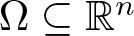 $\Omega\subseteq \mathbb{R}^n$, with $n\ge3$, then the L 2-norm of the singular term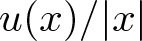 $u(x)/|x|$ is controlled by the L 2-norm of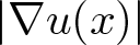 $|\nabla u(x)|$. More precisely, one has
 \begin{equation}
\int_{\Omega} |\nabla u(x)|^2\,\mathrm{d} x\geq \frac{(n-2)^2}{4}\int_{\Omega} \frac{|u(x)|^2}{|x|^2}\,\mathrm{d} x,\qquad \forall u\in C_0^\infty(\Omega).
\end{equation}
\begin{equation}
\int_{\Omega} |\nabla u(x)|^2\,\mathrm{d} x\geq \frac{(n-2)^2}{4}\int_{\Omega} \frac{|u(x)|^2}{|x|^2}\,\mathrm{d} x,\qquad \forall u\in C_0^\infty(\Omega).
\end{equation} Moreover, the above inequality is sharp, in the sense that the constant 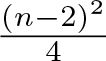 $\frac{(n-2)^2}{4}$ cannot be improved.
Due to the lack of an extremal function (for which equality holds), there exist various extensions and improvements of inequality (1), which turned out to be the fundamental building blocks of various results concerning elliptic problems; for comprehensive discussions, we refer to the monographs by Balinsky et al. [Reference Balinsky, Evans and Lewis1] and Ghoussoub and Moradifam [Reference Ghoussoub and Moradifam3]. Over the years, the mathematical community has answered many questions regarding Hardy-type inequalities, but several still remained open. The present paper focuses on such an unanswered problem, which is the issue of sharpness on non-compact and non-reversible Finsler manifolds with finite reversibility. Before presenting our main results, let us enlist some relevant facts.
The natural habitat for a Finslerian Hardy-type inequality is a Finsler metric measure manifold 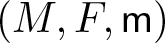 $(M,F,\mathsf{m})$ abbreviated by FMMM, which is a differentiable manifold M equipped with a smooth, positive-homogeneous metric F on the tangent bundle TM, and a smooth positive measure $\mathsf{m}$. When formulating Hardy-type inequalities in this setting, the expression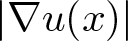 $|\nabla u (x)|$ is replaced by either $\max\{F^*(\pm Du)\}$ or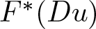 $F^*(Du)$, where $F^*$ is the dual metric of F, and Du denotes the derivative of u (see relations (8) and (15)). The quantity $|x|$ is typically replaced by a distance function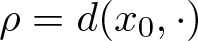 $\rho=d(x_0,\cdot)$ from a point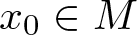 $x_0\in M$.
It turns out that three Finslerian quantities control the behaviour of Hardy inequalities:
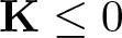
• The flag curvature K (see relation (18)), which is the natural Finslerian extension of the sectional curvature of Riemannian manifolds.
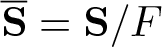
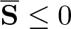
• The S-curvature S (see relation (19)), which is a pure Finslerian quantity measuring the rate of change of distortion along geodesics. For convenience, one can also use the reduced S-curvature $\overline{\mathbf{S}}=\mathbf{S}/F$.
• The reversibility, which is defined by
\begin{equation*}
\lambda_F(M)\stackrel{\textrm{def}}{=}\sup_{(x,y)\in TM} \mathbf{rev}(x,y), \quad\mbox{where}\quad \mathbf{rev}(x,y)=\frac{F(x,-y)}{F(x,y)}.
\end{equation*}Clearly
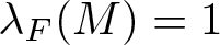
$1\le\lambda_F(M)\le +\infty$. The manifold is said to be reversible, if
$\lambda_F(M)=1$. In particular, every Riemannian metric is reversible.


The Finslerian version of the Hardy inequality (1), is due to Huang et al. [Reference Huang, Kristály and Zhao5, Theorem 1.4], where the authors showed that if 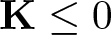 $\mathbf{K}\le 0$ and $\mathbf{S}\le0$, then one has
 \begin{equation}
\int_M \max\{F^*(\pm Du)\}^2\,\mathrm{d} \mathsf{m}\ge \left(\frac{n-2}{2}\right)^2\int_M\frac{u^2}{\rho^2}\,\mathrm{d} \mathsf{m},\quad \forall u\in C_0^\infty(M);
\end{equation}
\begin{equation}
\int_M \max\{F^*(\pm Du)\}^2\,\mathrm{d} \mathsf{m}\ge \left(\frac{n-2}{2}\right)^2\int_M\frac{u^2}{\rho^2}\,\mathrm{d} \mathsf{m},\quad \forall u\in C_0^\infty(M);
\end{equation} in addition, if F is reversible, then 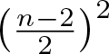 $ \left(\frac{n-2}{2}\right)^2$ is sharp. Since $\lambda_F(M)F^*(Du)\ge \max\{F^*(\pm Du)\}$, we also have
 \begin{equation}
\lambda_F(M)^2\int_M F^*(Du)^2\,\mathrm{d} \mathsf{m}\ge \left(\frac{n-2}{2}\right)^2\int_M\frac{u^2}{\rho^2}\,\mathrm{d} \mathsf{m},\quad \forall u\in C_0^\infty(M).
\end{equation}
\begin{equation}
\lambda_F(M)^2\int_M F^*(Du)^2\,\mathrm{d} \mathsf{m}\ge \left(\frac{n-2}{2}\right)^2\int_M\frac{u^2}{\rho^2}\,\mathrm{d} \mathsf{m},\quad \forall u\in C_0^\infty(M).
\end{equation} Note that if 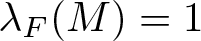 $\lambda_F(M)=1$, then inequalities (2) and (3) coincide. If $\lambda_F(M)=+\infty$, then left-hand side of the latter inequality blows up. In this case, the authors in [Reference Huang, Kristály and Zhao5, Example 6.2] showed that concerning the Funk metric with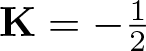 $\mathbf{K}=-\frac{1}{2}$,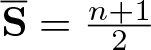 $\overline{\mathbf{S}}=\frac{n+1}{2}$, and $\lambda_F=+\infty$ one has
 \begin{equation*}
\inf_{u\in C_0^\infty(M)}\frac{\int_M {F^*}^2(Du)\,\mathrm{d} \mathsf{m}}{\int_M\frac{u^2}{\rho^2}\,\mathrm{d} \mathsf{m}}=0,
\end{equation*}
\begin{equation*}
\inf_{u\in C_0^\infty(M)}\frac{\int_M {F^*}^2(Du)\,\mathrm{d} \mathsf{m}}{\int_M\frac{u^2}{\rho^2}\,\mathrm{d} \mathsf{m}}=0,
\end{equation*}which aligns (in some sense) with inequality (3). We also refer to Kristály et al. [Reference Kristály, Li and Zhao7, Theorem 1.1] for additional results describing the failure of various functional inequalities.
In the remaining case when  $1 \lt \lambda_F(M) \lt \infty$, to the best of our knowledge, there is no evidence on the sharpness of (2) and (3). In fact, we are not aware of any particular examples where the sharpness persists. Our first main result is an affirmative example, based on the construction of suitable spaces presented below. Since the sharpness of (2) follows from the sharpness of (3), we only discuss the latter.
Consider the triple 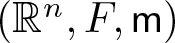 $(\mathbb{R}^n,F,\mathsf{m})$, where $F\colon \mathbb{R}^n\times \mathbb{R}^n\to [0,\infty)$ is defined by
 \begin{equation*}
F(x,y)=|y|-\frac{\langle x,y\rangle\theta}{|x|},\quad\text{if } x\ne O\quad\text{and}\quad F(O,y)=|y|,
\end{equation*}
\begin{equation*}
F(x,y)=|y|-\frac{\langle x,y\rangle\theta}{|x|},\quad\text{if } x\ne O\quad\text{and}\quad F(O,y)=|y|,
\end{equation*} for some 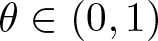 $\theta\in(0,1)$ and $\mathsf{m}$ stands for the Busemann–Hausdorff measure induced by F (see relation (14)). Here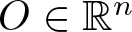 $O\in \mathbb{R}^n$ denotes the origin, $|\cdot|$ and $\langle\cdot,\cdot\rangle$ are the norm and the inner product in $\mathbb{R}^n$, respectively. Note that F is not a Finsler metric, since it is not continuous at the origin, but it has some remarkable properties, which could facilitate the proof of the sharpness of (3): The geodesics are straight lines. The reversibility is $\lambda_F(\mathbb{R}^n)=\frac{1+\theta}{1-\theta}=\lambda\in(1,\infty)$. If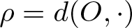 $\rho=d(O,\cdot)$, then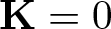 $\mathbf{K}=0$,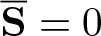 $\overline{\mathbf{S}}=0$, and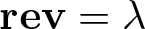 $\mathbf{rev}=\lambda$ along $\nabla\rho$, i.e., along the geodesics starting from O. Moreover, if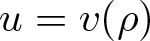 $u=v(\rho)$ with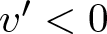 $v' \lt 0$, then one has $\lambda F^*(Du)=\max\{F^*(\pm Du)\}$.
To remedy the discontinuity at the O, we construct a family  $\mathcal{F}_{0,0,\lambda}=\{(\mathbb{R}^n,F_\varepsilon,\mathsf{m}_\varepsilon)\}_{\varepsilon \gt 0}$ of FMMMs, where
 \begin{equation*}
F_\varepsilon(x,y)=|y|-\frac{\langle x,y\rangle(|x|+2\varepsilon)\theta}{(|x|+\varepsilon)^2},
\end{equation*}
\begin{equation*}
F_\varepsilon(x,y)=|y|-\frac{\langle x,y\rangle(|x|+2\varepsilon)\theta}{(|x|+\varepsilon)^2},
\end{equation*} and  $\mathsf{m}_\varepsilon$ is the Busemann–Hausdorff measure induced by Fɛ. Note that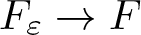 $F_\varepsilon\to F$ and $\mathsf{m}_\varepsilon\to \mathsf{m}$ (in densities) as ɛ → 0. Moreover, for every ɛ > 0, one has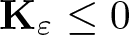 $\mathbf{K}_\varepsilon\le0$,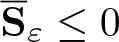 $\mathbf{\overline S}_\varepsilon\le0$, and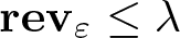 $\mathbf{rev}_\varepsilon\le\lambda$ along $\nabla\rho_\varepsilon$ (see theorem 4.1).
Using this family, our first result can be stated as follows; for a more general version, including weights and a general order p > 1, we refer to theorem 4.4.
Theorem 1.1. Let  $n\ge 3$,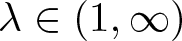 $\lambda\in (1,\infty)$. For every $(\mathbb{R}^n,F_\varepsilon,\mathsf{m}_\varepsilon)\in \mathcal{F}_{0,0,\lambda}$ and $u\in C_0^\infty(\mathbb{R}^n)$ one has
 \begin{equation}
\lambda^2\displaystyle\int_{\mathbb{R}^n} F_\varepsilon^*(Du)^2\,\mathrm{d} \mathsf{m}_\varepsilon\ge c_n\int_{\mathbb{R}^n}\frac{u^2}{\rho_\varepsilon^2}\,\mathrm{d} \mathsf{m}_\varepsilon,\quad\text{where}\quad c_n=\left(\frac{n-2}{2}\right)^2.
\end{equation}
\begin{equation}
\lambda^2\displaystyle\int_{\mathbb{R}^n} F_\varepsilon^*(Du)^2\,\mathrm{d} \mathsf{m}_\varepsilon\ge c_n\int_{\mathbb{R}^n}\frac{u^2}{\rho_\varepsilon^2}\,\mathrm{d} \mathsf{m}_\varepsilon,\quad\text{where}\quad c_n=\left(\frac{n-2}{2}\right)^2.
\end{equation} Moreover, cn is sharp in 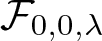 $\mathcal{F}_{0,0,\lambda}$, in the sense that it is the greatest constant with this property.
We highlight that 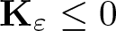 $\mathbf{K}_\varepsilon\le 0$ is not a global property on $(\mathbb{R}^n,F_\varepsilon,\mathsf{m}_\varepsilon)\in \mathcal{F}_{0,0,\lambda}$, i.e., for each point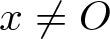 $x\ne O$, there exists a direction y (different from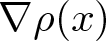 $\nabla\rho(x)$), such that $\mathbf{K}_\varepsilon(x,y) \gt 0$. Fortunately, this phenomenon does not affect our proofs. In fact, inequality (4) holds for arbitrary manifolds with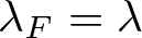 $\lambda_F=\lambda$, and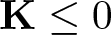 $\mathbf{K}\le 0$,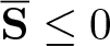 $\overline{\mathbf{S}}\le0$ along $\nabla\rho$ (see theorem 3.3), thus, the well-known global assumptions may be relaxed.
In the sequel, assuming strong negative curvature (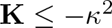 $\mathbf{K}\le-\kappa^2$, κ > 0 along $\nabla\rho$), we provide a similar construction as above. In this case, we focus on the celebrated spectral gap estimate of McKean [Reference McKean8]: if a Riemannian manifold has strong negative sectional curvature, then there exists a positive, domain independent lower bound for the first eigenvalue of the Laplacian (which is the fundamental tone of the fixed membrane). The Finslerian version of this result is due to Yin and He (see [Reference Yin and He14, Theorem 3.5]), which can be stated as follows (for p = 2): if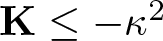 $\mathbf{K}\le -\kappa^2$ and $\sup_{TM} |\overline{\mathbf{S}}| \lt (n-1)\kappa$ for some κ > 0, and $\lambda_F(M) \lt \infty$, then
 \begin{equation}
\inf_{u\in W^{1,2}_0(M)}\frac{\int_M {F^*}(Du)^2\,\mathrm{d} \mathsf{m}}{\int_M|u|^2\,\mathrm{d} \mathsf{m}}\ge \left(\frac{(n-1)\kappa-\sup_{TM} |\overline{\mathbf{S}}|}{2\lambda}\right)^2.
\end{equation}
\begin{equation}
\inf_{u\in W^{1,2}_0(M)}\frac{\int_M {F^*}(Du)^2\,\mathrm{d} \mathsf{m}}{\int_M|u|^2\,\mathrm{d} \mathsf{m}}\ge \left(\frac{(n-1)\kappa-\sup_{TM} |\overline{\mathbf{S}}|}{2\lambda}\right)^2.
\end{equation} To prove a sharpness result concerning inequality (5), by perturbing the Klein metric on the Euclidean unit ball  $\mathbb{B}^n$, for arbitrary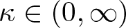 $\kappa\in(0,\infty)$,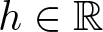 $h\in \mathbb{R}$, and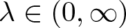 $\lambda\in(0,\infty)$, we construct a family $\mathcal{F}_{\kappa,h,\lambda}=\{(\mathbb{B}^n,F_\varepsilon,\mathsf{m}_\varepsilon)\}_{\varepsilon \gt 0}$ satisfying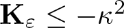 $\mathbf{K}_\varepsilon\le-\kappa^2$, $\overline{\mathbf{S}}_\varepsilon\le (n-1)h$, and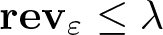 $\mathbf{rev}_\varepsilon\le \lambda$ along $\nabla\rho_\varepsilon$ (see theorem 5.1). This construction leads to our second main result, which can be stated as follows; for a more general version concerning the first eigenvalue of the p-Laplacian (with p > 1), we refer to theorem 5.4.
Theorem 1.2. Let  $n\ge 2$,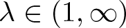 $\lambda\in (1,\infty)$, and $\kappa \gt h\ge0$. For every $(\mathbb{B}^n,F_\varepsilon,\mathsf{m}_\varepsilon)\in \mathcal{F}_{\kappa,h,\lambda}$ and $u\in C_0^\infty(\mathbb{B}^n)$ one has
 \begin{equation}
\lambda^2\displaystyle\int_{\mathbb{B}^n} F_\varepsilon^*(Du)^2\,\mathrm{d} \mathsf{m}_\varepsilon\ge c_{n,\kappa,h}\int_{\mathbb{B}^n} u^2 \,\mathrm{d} \mathsf{m}_\varepsilon,\quad\text{where}\quad c_{n,\kappa,h}=\left(\frac{(n-1)(\kappa-h)}{2}\right)^2.
\end{equation}
\begin{equation}
\lambda^2\displaystyle\int_{\mathbb{B}^n} F_\varepsilon^*(Du)^2\,\mathrm{d} \mathsf{m}_\varepsilon\ge c_{n,\kappa,h}\int_{\mathbb{B}^n} u^2 \,\mathrm{d} \mathsf{m}_\varepsilon,\quad\text{where}\quad c_{n,\kappa,h}=\left(\frac{(n-1)(\kappa-h)}{2}\right)^2.
\end{equation} Moreover,  $c_{n,\kappa,h}$ is sharp in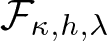 $\mathcal{F}_{\kappa,h,\lambda}$, in the sense that it is the greatest constant with this property.
Similarly to the previous case, 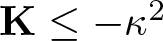 $\mathbf{K}\le-\kappa^2$ is not a global property. In addition, inequality (6) holds for arbitrary manifolds with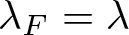 $\lambda_F=\lambda$, and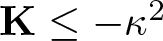 $\mathbf{K}\le -\kappa^2$,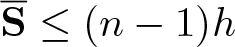 $\overline{\mathbf{S}}\le (n-1)h$ along $\nabla\rho$ (see theorem 3.4).
In order to establish inequalities (4) and (6) on general manifolds, we provide a Finslerian extension of the approach of Riccati pairs, developed by Kajántó et al. [Reference Kajántó, Kristály, Peter and Zhao6] in the Riemannian setting, which enables us to prove a general Hardy-type inequality:
 \begin{align*}\lambda^p \int_\Omega w(\rho)F(Du)^p\text{d}\mathsf{m}&\ge\int_\Omega w(\rho)\max\{F^*(\pm Du)\}^p\text{d}\mathsf{m}\\ &\ge \int_\Omega w(\rho)W(\rho)|u|^p\text{d} \mathsf{m},\quad \forall u\in C_0^\infty(\Omega),\end{align*}
 by simply solving a corresponding Riccati-type ODI, involving the parameters w, W, and p (see theorem 3.1). We note that the proof of this result inspired the basic idea of the construction of the families 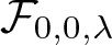 $\mathcal{F}_{0,0,\lambda}$ and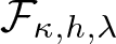 $\mathcal{F}_{\kappa,h,\lambda}$. Having this extension, we provide sufficient conditions for the sharpness of general Finslerian Hardy-type inequalities (obtained by Riccati pairs) on families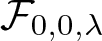 $\mathcal{F}_{0,0,\lambda}$ and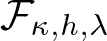 $\mathcal{F}_{\kappa,h,\lambda}$ (see theorems 4.3 and 5.3). Conceptually, the proof of the sharpness of a Hardy-type inequality relies on a suitable approximation (on the corresponding family) of the limit function of the given inequality, which is strongly related to the solution of the Riccati ODI (see remark 3.2(e)).
The paper is structured as follows: In §2 we present relevant definitions and results concerning Finsler geometry. In §3 we provide a Finslerian extension of Riccati pairs by proving theorem 3.1, which implies theorems 3.3 and 3.4. In §4 we address the issue of sharpness in case of non-positive flag curvature: theorem 4.1 presents the family 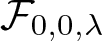 $\mathcal{F}_{0,0,\lambda}$, while theorem 4.3 provides sufficient conditions for the sharpness on them. As applications, we prove theorems 1.1 and 4.4. In §5 we proceed similarly in case of the strong negative flag curvature: theorem 5.1 presents the family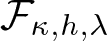 $\mathcal{F}_{\kappa,h,\lambda}$, while theorem 5.3 provides sufficient conditions for the sharpness on them. As applications, we prove theorems 1.2 and 5.4.
2. Preliminaries: elements from Finsler geometry
In this section, we recall various definitions and results from Finsler geometry that are relevant for our presentations. Here, we also fix our notation. For further details, we refer to the monographs by Bao et al. [Reference Bao, Chern and Shen2] and Shen [Reference Shen12].
2.1. Finsler manifolds
Let M be a smooth manifold with dimension  $n\ge 2$. At each point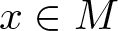 $x\in M$, the tangent space TxM consists of tangent vectors (or simply vectors) at x, while the cotangent space $T^*_xM$ consists of cotangent vectors (or covectors) at x, sometimes also referred to as one forms. These spaces are dual to each other, the canonical pairing between them is a bilinear form defined by
 \begin{equation*}
\langle\xi,y\rangle=\xi(y),\qquad \forall x\in M,\ y\in T_xM,\ \xi\in T^*_xM.
\end{equation*}
\begin{equation*}
\langle\xi,y\rangle=\xi(y),\qquad \forall x\in M,\ y\in T_xM,\ \xi\in T^*_xM.
\end{equation*} The tangent bundle TM is the collection of all tangent spaces, consisting of bound vectors, the cotangent bundle  $T^*M$ is the collection of all cotangent spaces, consisting of bound covectors. More precisely, we have
 \begin{equation*}
TM=\{(x,y):x\in M, y\in T_xM\}
\quad\mbox{and}\quad
T^*M=\{(x,\xi): x\in M, \xi\in T^*_xM\}.
\end{equation*}
\begin{equation*}
TM=\{(x,y):x\in M, y\in T_xM\}
\quad\mbox{and}\quad
T^*M=\{(x,\xi): x\in M, \xi\in T^*_xM\}.
\end{equation*} A vector field on M is a map that assigns to each point 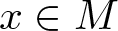 $x\in M$ a bound vector $(x,y)\in TM$. Similarly, a covector field assigns to each point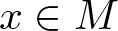 $x\in M$ a bound covector $(x,\xi )\in T^*M$.
Remark 2.1. For simplicity, we avoid the introduction of additional notation/letters for bound vectors and vector fields. If a statement involves a bound vector  $(x,y)\in TM$ or a vector field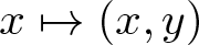 $x\mapsto (x,y)$, but the positional coordinate x is not particularly important, we simply omit x and formulate the statement using the bound vector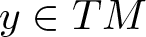 $y\in TM$ or the vector field y, respectively. Similarly, ξ may denote a covector, a bound covector, or a covector field. The specific underlying objects are always revealed by the context.
The couple (M, F) is said to be a Finsler manifold if the function  $F\colon TM\to[0,\infty)$ is a Finsler metric satisfying the following conditions:
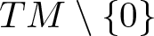
(i) Regularity: F(y) is smooth on
$TM\setminus\{0\}$, which consists of non-zero bound vectors;(ii) Positive homogeneity:
$F(\lambda y)=\lambda F(y)$, for every
$y\in TM$ and
$\lambda\ge0$;(iii) Strong convexity: For every
$y\in TM\setminus\{0\}$, the following quadratic form is positive definite:
(7)\begin{equation}
g_{y}(v,w)\stackrel{\textrm{def}}{=}\left.\frac{\partial^2}{\partial s\partial t}\left(\frac{1}{2}F(y+sv+tw)^2\right)\right|_{s=t=0},\qquad\forall v,w\in TM.
\end{equation}

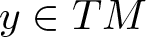



According to remark 2.1, we use both the notation F(y) and 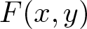 $F(x,y)$ depending on the context.
The reversibility of a Finsler manifold (M, F), introduced by Rademacher [Reference Rademacher10], is defined by
 \begin{equation*}
\lambda_F(M)\stackrel{\textrm{def}}{=}\sup_{x\in M}\sup_{y\in T_xM} \mathbf{rev}(x,y), \quad\mbox{where}\quad \mathbf{rev}(x,y)=\frac{F(x,-y)}{F(x,y)}.
\end{equation*}
\begin{equation*}
\lambda_F(M)\stackrel{\textrm{def}}{=}\sup_{x\in M}\sup_{y\in T_xM} \mathbf{rev}(x,y), \quad\mbox{where}\quad \mathbf{rev}(x,y)=\frac{F(x,-y)}{F(x,y)}.
\end{equation*} Clearly  $1\le\lambda_F(M)\le +\infty$. The manifold is said to be reversible, if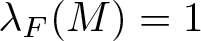 $\lambda_F(M)=1$.
The dual Finsler metric of F is the function  $F^*\colon T^*M\to[0,\infty)$, defined by
 \begin{equation}
F^*(\xi)\stackrel{\textrm{def}}{=} \sup_{y\in TM\setminus \{0\}}\frac{\langle\xi,y\rangle}{F(y)},\qquad \forall \xi\in T^*M,
\end{equation}
\begin{equation}
F^*(\xi)\stackrel{\textrm{def}}{=} \sup_{y\in TM\setminus \{0\}}\frac{\langle\xi,y\rangle}{F(y)},\qquad \forall \xi\in T^*M,
\end{equation} which is also a Finsler metric on M. The reversibility of 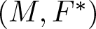 $(M,F^*)$ can be defined similarly by
 \begin{equation*}
\lambda_{F^*}(M)\stackrel{\textrm{def}}{=} \sup_{x\in M}\sup_{\xi\in T_x^*M} \mathbf{rev}^*(x,y), \quad\mbox{where}\quad \mathbf{rev}^*(x,y)=\frac{F^*(x,-\xi)}{F^*(x,\xi)}.
\end{equation*}
\begin{equation*}
\lambda_{F^*}(M)\stackrel{\textrm{def}}{=} \sup_{x\in M}\sup_{\xi\in T_x^*M} \mathbf{rev}^*(x,y), \quad\mbox{where}\quad \mathbf{rev}^*(x,y)=\frac{F^*(x,-\xi)}{F^*(x,\xi)}.
\end{equation*}In particular, according to e.g., Huang et al. [Reference Huang, Kristály and Zhao5, Lemma 2.1], one has
 \begin{equation}
\lambda_F(M)=\lambda_{F^*}(M).
\end{equation}
\begin{equation}
\lambda_F(M)=\lambda_{F^*}(M).
\end{equation} Using a Finsler metric F, one can define the length of a Lipschitz continuous curve  $c\colon [a,b]\to M$ by
 \begin{equation*}L(c)\stackrel{\textrm{def}}{=}\int_a^b F(\dot c(t)) \,\mathrm{d} t,\end{equation*}
 where the dot denotes the derivative with respect to t. Given two points  $x_0,x_1\in M$, the distance from x 0 to x 1 is defined by $d(x_0,x_1)= \inf_c L(c),$ where the infimum is taken over all Lipschitz continuous curves $c\colon [0,1]\to M$ with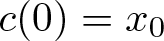 $c(0)=x_0$ and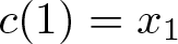 $c(1)=x_1$. In general, $d(x_0,x_1)\ne d(x_1,x_0)$, unless F is reversible.
If 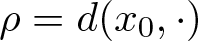 $\rho=d(x_0,\cdot)$ is the distance from a point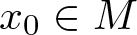 $x_0\in M$, then the eikonal equations hold $\!\,\mathrm{d}\mathsf{m}$-a.e. in M:
 \begin{equation}
F(\nabla \rho)=F^*(D\rho)=1.
\end{equation}
\begin{equation}
F(\nabla \rho)=F^*(D\rho)=1.
\end{equation} For fixed 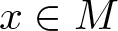 $x\in M$, the Legendre transform $\ell^*\colon T^*_xM\to T_xM$ assigns to each covector ξ the unique vector y, which minimizes the map
 \begin{equation*}
E^*(y)\stackrel{\textrm{def}}{=} \langle \xi, y\rangle - \frac{1}{2}F(y)^2.
\end{equation*}
\begin{equation*}
E^*(y)\stackrel{\textrm{def}}{=} \langle \xi, y\rangle - \frac{1}{2}F(y)^2.
\end{equation*} The minimizer 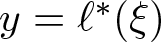 $y=\ell^*(\xi)$ can also be interpreted as the unique bound vector with the properties
 \begin{equation}
F(\ell^*(\xi))=F^*(\xi)\quad\mbox{and}\quad \langle \xi, \ell^*(\xi)\rangle =F(\ell^*(\xi))F^*(\xi).
\end{equation}
\begin{equation}
F(\ell^*(\xi))=F^*(\xi)\quad\mbox{and}\quad \langle \xi, \ell^*(\xi)\rangle =F(\ell^*(\xi))F^*(\xi).
\end{equation}Combining the properties from relation (11) yields
 \begin{equation}
\langle \xi,\ell^*(\xi)\rangle=F^*(\xi)^2, \qquad\forall \xi\in T^*_xM.
\end{equation}
\begin{equation}
\langle \xi,\ell^*(\xi)\rangle=F^*(\xi)^2, \qquad\forall \xi\in T^*_xM.
\end{equation} Similarly, the Legendre transform  $\ell\colon T_xM\to T^*_xM$ assigns to each vector y the unique covector ξ that minimizes the map
 \begin{equation*}
E(\xi)\stackrel{\textrm{def}}{=} \langle \xi, y\rangle - \frac{1}{2}F^*(\xi)^2.
\end{equation*}
\begin{equation*}
E(\xi)\stackrel{\textrm{def}}{=} \langle \xi, y\rangle - \frac{1}{2}F^*(\xi)^2.
\end{equation*} For the minimizer 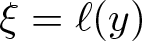 $\xi=\ell(y)$ similar relations hold as in (11) and (12). One also has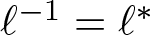 $\ell^{-1}=\ell^*$, hence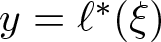 $y=\ell^*(\xi)$. Using the fact that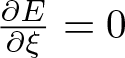 $\frac{\partial E}{\partial \xi}=0$, we obtain
 \begin{equation}
\ell^*(\xi)=F^*(\xi)\frac{\partial F^*(\xi)}{\partial \xi},\qquad
\forall \xi\in T_x^*M.
\end{equation}
\begin{equation}
\ell^*(\xi)=F^*(\xi)\frac{\partial F^*(\xi)}{\partial \xi},\qquad
\forall \xi\in T_x^*M.
\end{equation} Thus,  $\ell^*$ is positive homogeneous. Note that the definitions and properties of the Legendre transforms $\ell$ and $\ell^*$ naturally extend to bound vectors and vector fields. Moreover, using the conventions of remark 2.1, all of the above formulas are formally valid. We only need to make sure that the positional coordinates of y and ξ coincide, otherwise the canonical pairing does not make sense.
For every 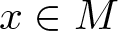 $x\in M$, there exists a local coordinate system $\{x^i\}$ defined on a coordinate neighbourhood of x. Denote by $\{\frac{\partial}{\partial x^i}\}$ and $\{\!\,\mathrm{d} x^i\}$ the induced basis on TxM and $T^*_xM$, respectively.
An FMMM 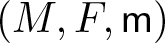 $(M,F, \mathsf{m})$ is a Finsler manifold equipped with a smooth positive measure $\mathsf{m}$. Unlike the Riemannian setting, there is no canonical measure in Finsler geometry. However, one often considers the Busemann–Hausdorff measure induced by F, which is given by
 \begin{equation}
\,\mathrm{d} \mathsf{m}_F\stackrel{\textrm{def}}{=}\sigma_F(x)\,\mathrm{d} x^1\wedge\ldots\wedge \,\mathrm{d} x^n,\quad\mbox{where}\quad \sigma_F(x)=\frac{\operatorname{vol}(\mathbb{B}^n)}{\operatorname{vol}(B_x(1))},
\end{equation}
\begin{equation}
\,\mathrm{d} \mathsf{m}_F\stackrel{\textrm{def}}{=}\sigma_F(x)\,\mathrm{d} x^1\wedge\ldots\wedge \,\mathrm{d} x^n,\quad\mbox{where}\quad \sigma_F(x)=\frac{\operatorname{vol}(\mathbb{B}^n)}{\operatorname{vol}(B_x(1))},
\end{equation}  $\operatorname{vol}(\cdot)$ denotes the Euclidean volume, $\mathbb{B}^n\subset \mathbb{R}^n$ is the Euclidean unit ball, while
 \begin{equation*}
B_x(1)=\{y\in T_xM: F(y) \lt 1\}.
\end{equation*}
\begin{equation*}
B_x(1)=\{y\in T_xM: F(y) \lt 1\}.
\end{equation*} The derivative of a smooth function  $u\colon M\to \mathbb{R}$ is a covector field defined by
 \begin{equation}
D u\stackrel{\textrm{def}}{=} \frac{\partial u}{\partial x^i}\,\mathrm{d} x^i.
\end{equation}
\begin{equation}
D u\stackrel{\textrm{def}}{=} \frac{\partial u}{\partial x^i}\,\mathrm{d} x^i.
\end{equation} The gradient of a smooth function  $u\colon M\to \mathbb{R}$ is a vector field that can be computed as
 \begin{equation}
\nabla u\stackrel{\textrm{def}}{=}\ell^*(D u).
\end{equation}
\begin{equation}
\nabla u\stackrel{\textrm{def}}{=}\ell^*(D u).
\end{equation} The divergence of a smooth vector field v with components  $(v^i)$ is given by
 \begin{equation*}
\mathrm{div}(v)\stackrel{\textrm{def}}{=} \sum_i \frac{1}{\sigma}\frac{\partial \sigma v^i}{\partial x^i}.
\end{equation*}
\begin{equation*}
\mathrm{div}(v)\stackrel{\textrm{def}}{=} \sum_i \frac{1}{\sigma}\frac{\partial \sigma v^i}{\partial x^i}.
\end{equation*}If p > 1, then the p-Laplacian of a smooth function u is
 \begin{equation*}
\Delta_{F,p} (u)\stackrel{\textrm{def}}{=} \mathrm{div}(F(\nabla u)^{p-2}\nabla u).
\end{equation*}
\begin{equation*}
\Delta_{F,p} (u)\stackrel{\textrm{def}}{=} \mathrm{div}(F(\nabla u)^{p-2}\nabla u).
\end{equation*}We note that for p = 2, the p-Laplacian is precisely the Finsler Laplacian
 \begin{equation*}\Delta_F (u) = \mathrm{div}(\nabla u).\end{equation*}
 We also notice that, if ρ is a distance function, then  $\Delta_{F,p}(\rho)=\Delta_F(\rho)$ holds $\!\,\mathrm{d}\mathsf{m}$-a.e. in M.
Finally, if u 1 and u 2 are smooth functions, both vanishing at the boundary, then the following integration by parts formula holds:
 \begin{equation}
\int_M u_1\Delta_F (u_2)\,\mathrm{d}\mathsf{m}=-\int_M \langle D u_1,\nabla u_2\rangle\,\mathrm{d}\mathsf{m},
\end{equation}
\begin{equation}
\int_M u_1\Delta_F (u_2)\,\mathrm{d}\mathsf{m}=-\int_M \langle D u_1,\nabla u_2\rangle\,\mathrm{d}\mathsf{m},
\end{equation}see e.g., Ohta and Sturm [Reference Ohta and Sturm9].
2.2. Curvatures and Laplace comparison
In the sequel, we recall the notions of the flag and S-curvature of an FMMM 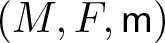 $(M,F,\mathsf{m})$, which can be interpreted more easily using tensors. According to the notation of the previous section, the fundamental tensor from relation (7) can be rewritten as
 \begin{equation*}
g_{(x,y)}=g_{ij}(x,y)\,\mathrm{d} x^i\,\mathrm{d} x^j,\quad\mbox{where}\quad g_{ij}(x,y)\stackrel{\textrm{def}}{=}\frac{1}{2}\frac{\partial^2 F(x,y)^2}{\partial y^i\partial y^j},\qquad \forall (x,y)\in TM.
\end{equation*}
\begin{equation*}
g_{(x,y)}=g_{ij}(x,y)\,\mathrm{d} x^i\,\mathrm{d} x^j,\quad\mbox{where}\quad g_{ij}(x,y)\stackrel{\textrm{def}}{=}\frac{1}{2}\frac{\partial^2 F(x,y)^2}{\partial y^i\partial y^j},\qquad \forall (x,y)\in TM.
\end{equation*}Note that, by convention, repeated indexes are automatically summed. The geodesic spray coefficients are defined as follows:
 \begin{equation*}
G^i(x,y)\stackrel{\textrm{def}}{=}\frac{1}{4}g^{il}(x,y)\left(2\frac{\partial g_{jl}(x,y)}{\partial x^k}- \frac{\partial g_{jk}(x,y)}{\partial x^l}\right)y^jy^k,\qquad \forall (x,y)\in TM.
\end{equation*}
\begin{equation*}
G^i(x,y)\stackrel{\textrm{def}}{=}\frac{1}{4}g^{il}(x,y)\left(2\frac{\partial g_{jl}(x,y)}{\partial x^k}- \frac{\partial g_{jk}(x,y)}{\partial x^l}\right)y^jy^k,\qquad \forall (x,y)\in TM.
\end{equation*} Recall that a smooth curve 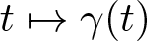 $t\mapsto \gamma(t)$ is geodesic if it satisfies the equation
 \begin{equation*}
\ddot \gamma^i(t)+2G^i(\gamma(t),\dot \gamma(t))=0.
\end{equation*}
\begin{equation*}
\ddot \gamma^i(t)+2G^i(\gamma(t),\dot \gamma(t))=0.
\end{equation*}The Riemannian curvature is defined by
 \begin{equation*}
R_{(x,y)}\stackrel{\textrm{def}}{=} R^i_k(x,y)\frac{\partial}{\partial x^i} \otimes dx^k, \qquad \forall (x,y)\in TM,
\end{equation*}
\begin{equation*}
R_{(x,y)}\stackrel{\textrm{def}}{=} R^i_k(x,y)\frac{\partial}{\partial x^i} \otimes dx^k, \qquad \forall (x,y)\in TM,
\end{equation*}where
 \begin{equation*}
R^i_k(x,y)\stackrel{\textrm{def}}{=} 2 \frac{\partial G^i(x,y)}{\partial x^k}-y^i\frac{\partial^2 G^i(x,y)}{\partial x^j\partial y^k}+2G^j(x,y)\frac{\partial^2 G^i(x,y)}{\partial y^j\partial y^k}-\frac{\partial G^i(x,y)}{\partial y^j}\frac{\partial G^j(x,y)}{\partial y^k}.
\end{equation*}
\begin{equation*}
R^i_k(x,y)\stackrel{\textrm{def}}{=} 2 \frac{\partial G^i(x,y)}{\partial x^k}-y^i\frac{\partial^2 G^i(x,y)}{\partial x^j\partial y^k}+2G^j(x,y)\frac{\partial^2 G^i(x,y)}{\partial y^j\partial y^k}-\frac{\partial G^i(x,y)}{\partial y^j}\frac{\partial G^j(x,y)}{\partial y^k}.
\end{equation*}The definition of flag curvature is as follows:
 \begin{equation}
\mathbf{K}(x,y,v)=\frac{g_{(x,y)}(R_{(x,y)}(v),v)}{g_{(x,y)}(y,y)g_{(x,y)}(v,v)-g_{(x,y)}(y,v)^2},\qquad \forall x\in M,\ y,v\in T_xM.
\end{equation}
\begin{equation}
\mathbf{K}(x,y,v)=\frac{g_{(x,y)}(R_{(x,y)}(v),v)}{g_{(x,y)}(y,y)g_{(x,y)}(v,v)-g_{(x,y)}(y,v)^2},\qquad \forall x\in M,\ y,v\in T_xM.
\end{equation}The name ‘flag’ refers to the plane spanned by the vectors y and v; the vector y is sometimes referred to as the flagpole.
The distortion is defined by
 \begin{equation*}
\tau(x,y)\stackrel{\textrm{def}}{=}\log\frac{\sqrt{\det g_{ij}(x,y)}}{\sigma(x)},\qquad \forall (x,y)\in TM.
\end{equation*}
\begin{equation*}
\tau(x,y)\stackrel{\textrm{def}}{=}\log\frac{\sqrt{\det g_{ij}(x,y)}}{\sigma(x)},\qquad \forall (x,y)\in TM.
\end{equation*}The S-curvature measures the rate of change of the distortion along geodesics, more precisely
 \begin{equation}
\mathbf{S}(x,y)=\left.\frac{\,\mathrm{d}}{\,\mathrm{d} t}\tau(\gamma(t),\dot\gamma(t))\right|_{t=0},\qquad \forall (x,y)\in TM,
\end{equation}
\begin{equation}
\mathbf{S}(x,y)=\left.\frac{\,\mathrm{d}}{\,\mathrm{d} t}\tau(\gamma(t),\dot\gamma(t))\right|_{t=0},\qquad \forall (x,y)\in TM,
\end{equation} where γ denotes the unique geodesic with 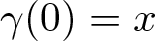 $\gamma(0)=x$ and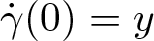 $\dot\gamma(0)=y$. For computational convenience (due to the homogeneity of degree zero), we prefer to use the reduced S-curvature defined by
 \begin{equation*}
\overline{\mathbf{S}}(x,y)=\frac{\mathbf{S}(x,y)}{F(x,y)},\quad \forall (x,y)\in TM,\ y\ne 0.
\end{equation*}
\begin{equation*}
\overline{\mathbf{S}}(x,y)=\frac{\mathbf{S}(x,y)}{F(x,y)},\quad \forall (x,y)\in TM,\ y\ne 0.
\end{equation*} For every  $\kappa\ge 0$, define $\mathbf{ct}_\kappa\colon (0,\infty)\to \mathbb{R}$ by
 \begin{equation*}{\mathbf{ct}}_\kappa(t)=
\begin{cases}
\frac{1}{t}, & \mbox{if } \kappa=0, \\
\kappa\coth(\kappa t), & \mbox{if } \kappa \gt 0. \\
\end{cases}
\end{equation*}
\begin{equation*}{\mathbf{ct}}_\kappa(t)=
\begin{cases}
\frac{1}{t}, & \mbox{if } \kappa=0, \\
\kappa\coth(\kappa t), & \mbox{if } \kappa \gt 0. \\
\end{cases}
\end{equation*} Our forthcoming arguments rely deeply on the following Laplace comparison theorem, which is a slight modification of the celebrated result by Wu and Xin [Reference Wu and Xin13, Theorem 5.1]. Here we only assume curvature conditions alongside the geodesics starting from some 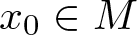 $x_0\in M$, which does not affect the original proof.
Theorem 2.2. Let (M, F) be a Finsler manifold and 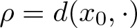 $\rho=d(x_0,\cdot)$ be the distance from a point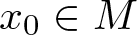 $x_0\in M$. Suppose that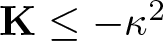 $\mathbf{K}\le -\kappa^2$ and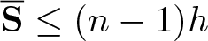 $\overline{\mathbf{S}}\le (n-1)h$ along $\nabla\rho$, for some $\kappa\ge 0$ and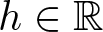 $h\in \mathbb{R}$. Then one has
 \begin{equation*}
\Delta_F (\rho)\ge (n-1)\mathbf{ct}_\kappa(\rho)-(n-1)h.
\end{equation*}
\begin{equation*}
\Delta_F (\rho)\ge (n-1)\mathbf{ct}_\kappa(\rho)-(n-1)h.
\end{equation*} Moreover, equality holds if and only if 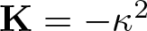 $\mathbf{K}= -\kappa^2$ and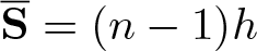 $\overline{\mathbf{S}}= (n-1)h$, along $\nabla\rho$.
2.3. Special Finsler metrics
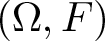
A Finsler metric on 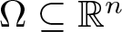 $\Omega\subseteq\mathbb{R}^n$ is said to be projectively flat if the geodesics are straight (Euclidean) lines as point sets. Due to Rapcsák [Reference Rapcsák11], we have the following characterization.
Theorem 2.3. Let  $F\colon T\Omega\to[0,\infty)$ be a Finlser metric on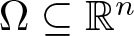 $\Omega\subseteq \mathbb{R}^n$. The following conditions are equivalent:
(i) The Finsler space
$(\Omega,F)$ is projectively flat.(ii) The geodesic coefficients of F are given by
(20)\begin{equation}
G^i(x,y)=P(x,y)y^i,\quad\mbox{where}\quad P(x,y)=\frac{1}{2F(x,y)}\cdot \frac{\partial F(x,y)}{\partial x^k}y^k.
\end{equation}(iii) The metric F satisfies
(21)\begin{equation}
\frac{\partial^2 F(x,y)}{\partial x^k\partial y^i}y^k=\frac{\partial F(x,y)}{\partial x^i},\quad \forall i\in\{1,\dots,n\}.
\end{equation}


The following proposition is useful for computing the flag and S-curvature of a projectively flat metric. For the proof, we refer to Shen [Reference Shen12, Sections 6.3 and 7.3]
Proposition 2.4. Suppose that 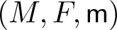 $(M,F,\mathsf{m})$ is an FMMM equipped with a projectively flat Finsler metric F and a smooth positive measure $\mathsf{m}$ having density σ. The flag and S-curvature can be computed as follows:
 \begin{align*}
\mathbf{K}(x,y) & =\frac{1}{F(x,y)^2}\left(P(x,y)^2-\frac{\partial P(x,y)}{\partial x^i}y^i\right), \\
\mathbf{S}(x,y) & =\frac{\partial G^i(x,y)}{\partial y^i}-\frac{y^i}{\sigma(x)}\frac{\partial \sigma(x)}{\partial x^i},
\end{align*}
\begin{align*}
\mathbf{K}(x,y) & =\frac{1}{F(x,y)^2}\left(P(x,y)^2-\frac{\partial P(x,y)}{\partial x^i}y^i\right), \\
\mathbf{S}(x,y) & =\frac{\partial G^i(x,y)}{\partial y^i}-\frac{y^i}{\sigma(x)}\frac{\partial \sigma(x)}{\partial x^i},
\end{align*}where P and Gi are given by relation (20). Note that in this case K only depends on x and y.
In the sequel, we consider a special class of Finsler spaces, called Randers spaces, which are important examples of Finsler manifolds: In many cases, they help us to observe and investigate conceptual differences between Riemannian and Finsler geometries. A Randers space is a differentiable manifold M endowed with a special Finsler metric  $F\colon TM\to[0,\infty)$ called Randers metric, which is defined by
 \begin{equation}
F(x,y)=\sqrt{a_{ij}(x)y^iy^j}+b_i(x)y^i,
\end{equation}
\begin{equation}
F(x,y)=\sqrt{a_{ij}(x)y^iy^j}+b_i(x)y^i,
\end{equation} where  $a_{ij}(x)\,\mathrm{d} x^i\,\mathrm{d} x^j$ is a Riemannian metric,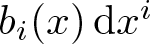 $b_i(x)\,\mathrm{d} x^i$ is a a one-form, such that
 \begin{equation*}
\|b(x)\|_a\stackrel{\textrm{def}}{=}\sqrt{a^{ij}(x)b_i(x)b_j(x)} \lt 1, \quad\forall x\in M,
\end{equation*}
\begin{equation*}
\|b(x)\|_a\stackrel{\textrm{def}}{=}\sqrt{a^{ij}(x)b_i(x)b_j(x)} \lt 1, \quad\forall x\in M,
\end{equation*} and 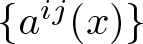 $\{a^{ij}(x)\}$ denotes the inverse of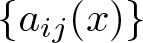 $\{a_{ij}(x)\}$. The density of the Busemann–Hausdorff measure induced by a Raders metric F is given by
 \begin{equation}
\sigma_F(x)=(1-\|b(x)\|_a^2)^\frac{n+1}{2}\sqrt{\det a_{ij}(x)}.
\end{equation}
\begin{equation}
\sigma_F(x)=(1-\|b(x)\|_a^2)^\frac{n+1}{2}\sqrt{\det a_{ij}(x)}.
\end{equation}For later use, define the Kronecker delta by
 \begin{equation}
\delta_{ij}\stackrel{\textrm{def}}{=} \begin{cases}
1, & \mbox{if } i=j, \\
0, & \mbox{if } i\ne j.
\end{cases}
\end{equation}
\begin{equation}
\delta_{ij}\stackrel{\textrm{def}}{=} \begin{cases}
1, & \mbox{if } i=j, \\
0, & \mbox{if } i\ne j.
\end{cases}
\end{equation}The following observation proves to be useful in the sequel.
Remark 2.5. Let F be a Randers metric given by (22). It the Riemannian metric  $\overline F(x,y)=\sqrt{a_{ij}(x)y^iy^j}$ satisfies (21), and $b_i\,\mathrm{d} x^i=D\beta(x)$ for some smooth function β, then F satisfies (21) as well. Thus, according to theorem 2.3 the metric F is projectively flat. The claim easily follows from the symmetry of second-order partial derivatives of the smooth function β.
3. A Finslerian extension of Riccati pairs
In this section, we present a Finslerian extension of the approach of Riccati pairs, established by Kajántó et al. [Reference Kajántó, Kristály, Peter and Zhao6] in the Riemannian setting, which enables us to prove a Hardy-type inequality, by simply solving a corresponding Riccati-type ordinary differential inequality. The key ideas of the proof are similar to [Reference Kajántó, Kristály, Peter and Zhao6], however, some extra workarounds are needed due to the specificities of the Finsler geometry. Our extension can be stated as follows.
Theorem 3.1. Let 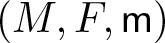 $(M,F,\mathsf{m})$ be a forward complete, non-compact FMMM, with dimension $n\ge 2$ and reversibility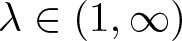 $\lambda\in(1,\infty)$. Let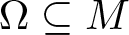 $\Omega\subseteq M$ be a domain, p > 1,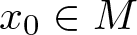 $x_0\in M$ and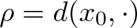 $\rho=d(x_0,\cdot)$ the distance from x 0. Suppose that the couple (L, W) is a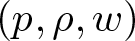 $(p,\rho,w)$-Riccati pair in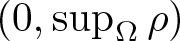 $(0,\sup_\Omega\rho)$ that is
(C1)
$L,W,w\colon(0,\sup_\Omega\rho)\to(0,\infty)$ such that
$L,W$ are continuous and w is of class C 1;(C2)
$\Delta_F \rho\geq L(\rho)$ in the distributional sense in Ω;(C3) there exists a function
$G\colon(0,\sup_\Omega\rho)\to(0,\infty)$ of class C 1 such that the following Riccati ODI holds:
(25)\begin{align}
\kern-20pt (G(t)w(t))'+G(t)w(t)L(t)-(p-1)G(t)^{p'}w(t)\geq W(t)w(t), \,\,\,\,\,\forall t\in (0,\sup\nolimits_\Omega\rho),
\end{align}





where 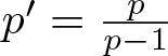 $p'=\frac{p}{p-1}$. Then for every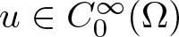 $u\in C_0^\infty(\Omega)$ one has
 \begin{align}
\lambda^p\int_\Omega w(\rho)F^*(Du)^p\,\mathrm{d} \mathsf{m}\ge \int_\Omega w(\rho)\max\{F^*(\pm Du)\}^p\,\mathrm{d} \mathsf{m} & \ge \int_\Omega w(\rho)W(\rho)|u|^p\,\mathrm{d} \mathsf{m}.
\end{align}
\begin{align}
\lambda^p\int_\Omega w(\rho)F^*(Du)^p\,\mathrm{d} \mathsf{m}\ge \int_\Omega w(\rho)\max\{F^*(\pm Du)\}^p\,\mathrm{d} \mathsf{m} & \ge \int_\Omega w(\rho)W(\rho)|u|^p\,\mathrm{d} \mathsf{m}.
\end{align}Proof. The convexity of the map 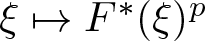 $\xi\mapsto F^*(\xi)^p$ implies
 \begin{equation}
F^*(\xi)^p\ge F^*(\eta)^p +\left\langle \xi-\eta, \frac{\partial}{\partial \eta}F^*(\eta)^p\right\rangle,\qquad \forall \xi,\eta\in T^*\Omega.
\end{equation}
\begin{equation}
F^*(\xi)^p\ge F^*(\eta)^p +\left\langle \xi-\eta, \frac{\partial}{\partial \eta}F^*(\eta)^p\right\rangle,\qquad \forall \xi,\eta\in T^*\Omega.
\end{equation}By using the chain rule and the properties of Legendre transforms (see relations (12) and (13)), we obtain
 \begin{equation}
F^*(\xi)^p\ge p F^*(\eta)^{p-2}\langle \xi,\ell^*(\eta)\rangle-(p-1)F^*(\eta)^p,\qquad \forall \xi,\eta\in T^*\Omega.
\end{equation}
\begin{equation}
F^*(\xi)^p\ge p F^*(\eta)^{p-2}\langle \xi,\ell^*(\eta)\rangle-(p-1)F^*(\eta)^p,\qquad \forall \xi,\eta\in T^*\Omega.
\end{equation}Introduce the notation
 \begin{equation*}
\operatorname{sgn}(t) = \begin{cases}
1 & \text{if }t \gt 0, \\
0 & \text{if } t=0, \\
-1 & \text{if } t \lt 0,
\end{cases}
\end{equation*}
\begin{equation*}
\operatorname{sgn}(t) = \begin{cases}
1 & \text{if }t \gt 0, \\
0 & \text{if } t=0, \\
-1 & \text{if } t \lt 0,
\end{cases}
\end{equation*}and let us make in inequality (28) the following choices:
 \begin{equation}
\xi=-\operatorname{sgn}(u)Du\quad\mbox{and}\quad\eta=\operatorname{sgn}(u)G(\rho)^\frac{1}{p-1}u D \rho.
\end{equation}
\begin{equation}
\xi=-\operatorname{sgn}(u)Du\quad\mbox{and}\quad\eta=\operatorname{sgn}(u)G(\rho)^\frac{1}{p-1}u D \rho.
\end{equation} On the one hand, the positive homogeneity of  $F^*$ implies
 \begin{align*}
p F^*(\eta)^{p-2} & =pG(\rho)^\frac{p-2}{p-1}F^*(D\rho)^{p-2}|u|^{p-2}, \\
(p-1)F^*(\eta)^p & =(p-1)G(\rho)^{p'}F^*(D\rho)^p|u|^{p}.
\end{align*}
\begin{align*}
p F^*(\eta)^{p-2} & =pG(\rho)^\frac{p-2}{p-1}F^*(D\rho)^{p-2}|u|^{p-2}, \\
(p-1)F^*(\eta)^p & =(p-1)G(\rho)^{p'}F^*(D\rho)^p|u|^{p}.
\end{align*} On the other hand, since  $\ell^*$ is positive homogeneous and the canonical pairing is bilinear, we have
 \begin{equation*}
\langle \xi,\ell^*(\eta)\rangle=-G(\rho)^\frac{1}{p-1}u\langle Du, \ell^*(D\rho)\rangle.
\end{equation*}
\begin{equation*}
\langle \xi,\ell^*(\eta)\rangle=-G(\rho)^\frac{1}{p-1}u\langle Du, \ell^*(D\rho)\rangle.
\end{equation*}Thus, the chain rule yields
 \begin{equation*}
pF^*(\eta)^{p-2}\langle \xi,\ell^*(\eta)\rangle=-G(\rho)F^*(D\rho)^{p-2}\langle D(|u|^p), \ell^*(D\rho)\rangle.
\end{equation*}
\begin{equation*}
pF^*(\eta)^{p-2}\langle \xi,\ell^*(\eta)\rangle=-G(\rho)F^*(D\rho)^{p-2}\langle D(|u|^p), \ell^*(D\rho)\rangle.
\end{equation*}By the above computations, it follows that
 \begin{equation*}
F^*(-\operatorname{sgn}(u)Du)^p\ge -G(\rho)F^*(D\rho)^{p-2}\langle D(|u|^p), \ell^*(D\rho)\rangle-(p-1)G(\rho)^{p'}F^*(D\rho)^p|u|^{p}.
\end{equation*}
\begin{equation*}
F^*(-\operatorname{sgn}(u)Du)^p\ge -G(\rho)F^*(D\rho)^{p-2}\langle D(|u|^p), \ell^*(D\rho)\rangle-(p-1)G(\rho)^{p'}F^*(D\rho)^p|u|^{p}.
\end{equation*} Multiplying both sides by 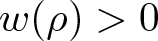 $w(\rho) \gt 0$ and integrating over Ω yields
 \begin{align}
\int_\Omega w(\rho)F^*(-\operatorname{sgn}(u)Du)^p\,\mathrm{d} \mathsf{m}
& \ge -\int_\Omega w(\rho)G(\rho)F^*(D\rho)^{p-2}\langle D (|u|^p), \ell^*(D\rho)\rangle\,\mathrm{d} \mathsf{m}\nonumber \\
& \qquad -(p-1)\int_\Omega w(\rho)G(\rho)^{p'}F^*(D\rho)^p|u|^{p}\,\mathrm{d} \mathsf{m}.
\end{align}
\begin{align}
\int_\Omega w(\rho)F^*(-\operatorname{sgn}(u)Du)^p\,\mathrm{d} \mathsf{m}
& \ge -\int_\Omega w(\rho)G(\rho)F^*(D\rho)^{p-2}\langle D (|u|^p), \ell^*(D\rho)\rangle\,\mathrm{d} \mathsf{m}\nonumber \\
& \qquad -(p-1)\int_\Omega w(\rho)G(\rho)^{p'}F^*(D\rho)^p|u|^{p}\,\mathrm{d} \mathsf{m}.
\end{align} First, by the eikonal equation (10), the factors 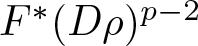 $F^*(D\rho)^{p-2}$ and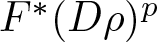 $F^*(D\rho)^p$ can be omitted. Second, the integration by parts formula (17) for $u_1=w(\rho)G(\rho)|u|^p$ and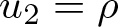 $u_2=\rho$ implies
 \begin{align*}
&\int_\Omega (w(\rho)G(\rho)\Delta_F\rho) |u|^p\,\mathrm{d} \mathsf{m}=-\int_\Omega(w(\rho)G(\rho))'\langle D\rho,\nabla\rho\rangle |u|^p\, \\& \mathrm{d} \mathsf{m}- \int_\Omega w(\rho)G(\rho)\langle D(|u|^p),\nabla\rho\rangle\,\mathrm{d} \mathsf{m}.
\end{align*}
\begin{align*}
&\int_\Omega (w(\rho)G(\rho)\Delta_F\rho) |u|^p\,\mathrm{d} \mathsf{m}=-\int_\Omega(w(\rho)G(\rho))'\langle D\rho,\nabla\rho\rangle |u|^p\, \\& \mathrm{d} \mathsf{m}- \int_\Omega w(\rho)G(\rho)\langle D(|u|^p),\nabla\rho\rangle\,\mathrm{d} \mathsf{m}.
\end{align*} Next, since  $\nabla\rho=\ell^*(D\rho)$, by relation (11) and the eikonal equation, the factor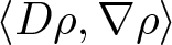 $\langle D\rho,\nabla\rho\rangle$ can also be omitted. Thus, inequality (30) can be rewritten as
 \begin{align*}
&\int_\Omega w(\rho) F^*(-\operatorname{sgn}(u)Du)^p\,\mathrm{d} \mathsf{m} \\ & \quad \ge \int_\Omega \left((w(\rho)G(\rho))'+w(\rho)G(\rho)\Delta_F\rho- (p-1)w(\rho)G(\rho)^{p'}\right)|u|^p\,\mathrm{d} \mathsf{m}.
\end{align*}
\begin{align*}
&\int_\Omega w(\rho) F^*(-\operatorname{sgn}(u)Du)^p\,\mathrm{d} \mathsf{m} \\ & \quad \ge \int_\Omega \left((w(\rho)G(\rho))'+w(\rho)G(\rho)\Delta_F\rho- (p-1)w(\rho)G(\rho)^{p'}\right)|u|^p\,\mathrm{d} \mathsf{m}.
\end{align*}Next, since w and G are positive, condition (C2) implies
 \begin{align*}
&\int_\Omega w(\rho)F^*(-\operatorname{sgn}(u)Du)^p\,\mathrm{d} \mathsf{m}\\& \quad \ge \int_\Omega \left((w(\rho)G(\rho))'+w(\rho)G(\rho)L(\rho)-(p-1)w(\rho)G(\rho)^{p'}\right)|u|^p\,\mathrm{d} \mathsf{m},
\end{align*}
\begin{align*}
&\int_\Omega w(\rho)F^*(-\operatorname{sgn}(u)Du)^p\,\mathrm{d} \mathsf{m}\\& \quad \ge \int_\Omega \left((w(\rho)G(\rho))'+w(\rho)G(\rho)L(\rho)-(p-1)w(\rho)G(\rho)^{p'}\right)|u|^p\,\mathrm{d} \mathsf{m},
\end{align*}thus, applying the Riccati ODI (25) from condition (C3) yields
 \begin{equation*}
\int_\Omega w(\rho)F^*(-\operatorname{sgn}(u)Du)^p\,\mathrm{d} \mathsf{m}\ge \int_\Omega w(\rho)W(\rho)\,\mathrm{d} \mathsf{m}.
\end{equation*}
\begin{equation*}
\int_\Omega w(\rho)F^*(-\operatorname{sgn}(u)Du)^p\,\mathrm{d} \mathsf{m}\ge \int_\Omega w(\rho)W(\rho)\,\mathrm{d} \mathsf{m}.
\end{equation*} Finally, since  $\lambda_F(M)=\lambda_{F^*}(M)=\lambda$ (see relation (9)), the following chain of inequalities hold:
 \begin{equation}
\lambda F^*(Du)\ge \max\{F^*(\pm Du)\}\ge F^*(-\operatorname{sgn}(u)Du),
\end{equation}
\begin{equation}
\lambda F^*(Du)\ge \max\{F^*(\pm Du)\}\ge F^*(-\operatorname{sgn}(u)Du),
\end{equation}which combined with the positivity of w finishes the proof.
Several comments are in order.
(a) The above theorem, in fact, extends the combination of theorems 3.1 and 3.2 of [Reference Kajántó, Kristály, Peter and Zhao6]. For a more straightforward presentation, we imposed more simpler but stricter conditions on the parameters: we assumed smoothness instead of local integrability, eliminated an extra parameter, considered only distances from a point, and so on. However, if the applications require, one can easily relax these conditions, without affecting the proof.
(b) Conceptually, theorem 3.1 has the same benefit as its Riemannian counterpart: It reduces the proof of a Hardy inequality from the relation (26) to the solvability of the Riccati ODI (25). In addition, the Riemannian applications presented in [Reference Kajántó, Kristály, Peter and Zhao6] gain natural Finslerian extensions: One only needs to formally replace
$|\nabla u|$ by either
$\max\{F^*(\pm Du)\}$ or
$\lambda F^*(Du)$ in the corresponding inequalities.(c) In [Reference Kajántó, Kristály, Peter and Zhao6], the authors also provided an alternative formulation of the above result called multiplicative form, which allows us to consider uncertainty principles (such as the Heisenberg–Pauli–Weyl uncertainty principle and the Hydrogen uncertainty principle) and Caffarelli–Kohn–Nirenberg inequalities. The proof relies on a scaling argument, which can also be adapted to the Finsler setting. By doing this, one can provide Finslerian extensions to the aforementioned inequalities. The details are left to the interested reader.
(d) Theorem 3.1 highlights the effect of K,
$\overline{\mathbf{S}}$, and rev on Hardy inequalities: Condition (C2) is ensured by the Laplace comparison theorem (see theorem 2.2), the exact form of L depends on the upper bound of the flag curvature K and the reduced S-curvature
$\overline{\mathbf{S}}$ along the geodesics starting from x 0. The effect of reversibility is made precise in relation (31).(e) Theorem 3.1 also gives some hints about the sharpness of Hardy-type inequalities: one can expect the inequalities of (26) to be close to the equality if the inequality of condition (C2), the inequalities from (31), and the convexity inequality (27) are close to equality. The first two of them are related to the geometry of the ambient space (see also theorem 2.2), while the third provides information concerning u.
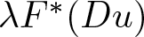
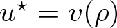
Define the limit function
$u^\star$ of the Hardy inequality (26), as a radially symmetric function
$u^\star=v(\rho)$ for some
$v\colon(0,\sup_\Omega\rho)\to \mathbb{R}$, for which
$\xi=\eta$ in relation (29), and thus inequality (27) becomes an equality. Then we obtain
\begin{equation*}
-(\log(v(t)))'=-\frac{{v}'(t)}{v(t)}=G(t)^\frac{1}{p-1},\quad \forall t\in(0,\sup\nolimits_\Omega\rho).
\end{equation*}For
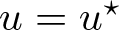
$u=u^\star$ the integrals of the inequality (26) are not convergent (there exists no extremal function), but considering its approximations/truncations may yield sharpness. To get close to the equality in (C2) and (31), in §4.1 and §5.1, we construct some suitable spaces for these approximations. We note, however, that a general proof of sharpness (if exists) would not require such constructions.







3.1. Applications
In this section, by applying theorem 3.1, we prove a Finslerian version of a weighted Hardy inequality and a McKean-type spectral gap estimate. We note that our choice of parameters agrees with the corresponding Riemannian counterparts from [Reference Kajántó, Kristály, Peter and Zhao6]. The first application can be stated as follows.
Theorem 3.3. Let 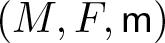 $(M,F,\mathsf{m})$ be a forward complete, non-compact FMMM, with dimension $n\ge 3$, and reversibility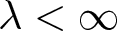 $\lambda \lt \infty$. Let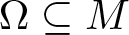 $\Omega\subseteq M$ be a domain,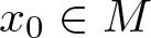 $x_0\in M$ and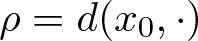 $\rho=d(x_0,\cdot)$ the distance from x 0. Suppose that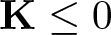 $\mathbf{K}\le 0$,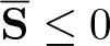 $\overline{\mathbf{S}}\le 0$ along $\nabla \rho$. Let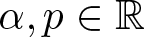 $\alpha,p\in \mathbb{R}$ such that $1 \lt p \lt n+\alpha$. Then for every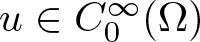 $u\in C_0^\infty(\Omega)$ one has
 \begin{equation}
\lambda^p\displaystyle\int_\Omega \rho^\alpha\cdot F^*(Du)^p\,\mathrm{d} \mathsf{m} \ge\displaystyle\int_\Omega \rho^\alpha\cdot \max\{F^*(\pm Du)\}^p\,\mathrm{d} \mathsf{m} \ge c_{n,p,\alpha}\displaystyle\int_\Omega \rho^\alpha\frac{|u|^p}{\rho^p}\,\mathrm{d} \mathsf{m},
\end{equation}
\begin{equation}
\lambda^p\displaystyle\int_\Omega \rho^\alpha\cdot F^*(Du)^p\,\mathrm{d} \mathsf{m} \ge\displaystyle\int_\Omega \rho^\alpha\cdot \max\{F^*(\pm Du)\}^p\,\mathrm{d} \mathsf{m} \ge c_{n,p,\alpha}\displaystyle\int_\Omega \rho^\alpha\frac{|u|^p}{\rho^p}\,\mathrm{d} \mathsf{m},
\end{equation} where 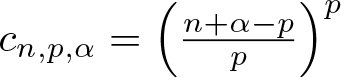 $c_{n,p,\alpha}=\left(\frac{n+\alpha-p}{p}\right)^p$.
Proof. In theorem 3.1 let us choose  $\Omega=M\setminus\{x_0\}$, as well as,
 \begin{align*}
&w(t)=t^\alpha,\quad L(t)=\frac{n-1}{t},\quad W(t)= c_{n,p,\alpha}\cdot \frac{1}{t^p} ,\\ & \quad \mbox{and } G(t)=(c_{n,p,\alpha})^\frac{p-1}{p}\cdot\frac{1}{t^{p-1}},\quad\forall t \gt 0.\end{align*}
\begin{align*}
&w(t)=t^\alpha,\quad L(t)=\frac{n-1}{t},\quad W(t)= c_{n,p,\alpha}\cdot \frac{1}{t^p} ,\\ & \quad \mbox{and } G(t)=(c_{n,p,\alpha})^\frac{p-1}{p}\cdot\frac{1}{t^{p-1}},\quad\forall t \gt 0.\end{align*} Obviously, the above functions satisfy (C1). The Laplace comparison (see theorem 2.2) implies that (C2) holds as well. By a simple computation, the Riccati ODI of condition (C3) is verified with equality. Thus, theorem 3.1 implies that inequality (32) holds for every  $u\in C_0^\infty(M\setminus\{x_0\})$. Finally, we use a result from capacity theory (see e.g., [Reference Kajántó, Kristály, Peter and Zhao6, Remark 4.2]): Since the p-capacity of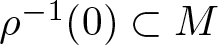 $\rho^{-1}(0)\subset M$ is zero, thus, inequality (32) holds for every $u\in C_0^\infty(M)$ as well.
We notice that Zhao in [Reference Zhao15, Theorem 1.1] showed that if 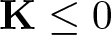 $\mathbf{K}\le 0$ (globally) and $\mathbf{S}\ge0$ along $\nabla \overleftarrow\rho$, where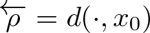 $\overleftarrow\rho=d(\cdot, x_0)$, then one has
 \begin{equation*}
\int_\Omega \overleftarrow\rho^\alpha\cdot \max\{F^*(\pm Du)\}^2\,\mathrm{d} \mathsf{m}\ge c_{n,p,\alpha}\int_\Omega\overleftarrow\rho^\alpha\frac{|u|^p}{\overleftarrow\rho^p}\,\mathrm{d} \mathsf{m},\quad \forall u\in C_0^\infty(M);
\end{equation*}
\begin{equation*}
\int_\Omega \overleftarrow\rho^\alpha\cdot \max\{F^*(\pm Du)\}^2\,\mathrm{d} \mathsf{m}\ge c_{n,p,\alpha}\int_\Omega\overleftarrow\rho^\alpha\frac{|u|^p}{\overleftarrow\rho^p}\,\mathrm{d} \mathsf{m},\quad \forall u\in C_0^\infty(M);
\end{equation*} additionally, if F is reversible, then the constant  $c_{n,p,\alpha}$ is sharp. Since, $\mathbf{S}\ge 0$ along $\nabla\overleftarrow\rho$ if and only if $\mathbf{S}\le 0$ along $\nabla \rho$, this result perfectly aligns with inequality (32).
The second application can be stated as follows.
Theorem 3.4. Let 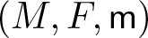 $(M,F,\mathsf{m})$ be a forward complete, non-compact FMMM, with dimension $n\ge 3$, and reversibility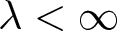 $\lambda \lt \infty$. Let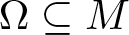 $\Omega\subseteq M$ be a domain,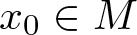 $x_0\in M$ and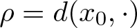 $\rho=d(x_0,\cdot)$ the distance from x 0. Suppose that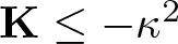 $\mathbf{K}\le -\kappa^2$,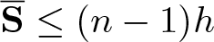 $\overline{\mathbf{S}}\le (n-1)h$ along $\nabla \rho$, for some $\kappa \gt h\ge0$, and let p > 1. Then for every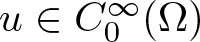 $u\in C_0^\infty(\Omega)$ one has
 \begin{equation}
\lambda^p\int_\Omega F^*(Du)^p\,\mathrm{d} \mathsf{m} \ge\int_\Omega \max\{F^*(\pm Du)\}^p\,\mathrm{d} \mathsf{m} \ge c_{n,p,\kappa,h} \int_\Omega |u|^p\,\mathrm{d} \mathsf{m},
\end{equation}
\begin{equation}
\lambda^p\int_\Omega F^*(Du)^p\,\mathrm{d} \mathsf{m} \ge\int_\Omega \max\{F^*(\pm Du)\}^p\,\mathrm{d} \mathsf{m} \ge c_{n,p,\kappa,h} \int_\Omega |u|^p\,\mathrm{d} \mathsf{m},
\end{equation} where  $c_{n,p,\kappa,h}=\left(\frac{(n-1)(\kappa-h)}{p}\right)^p$.
Proof. In theorem 3.1 let us choose 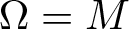 $\Omega=M$, as well as
 \begin{equation*}
w(t)\equiv 1, \quad L(t)\equiv (n-1)(\kappa-h) , \quad W(t)\equiv c_{n,p,\kappa,h},\quad\mbox{and}\quad G(t)\equiv (c_{n,p,\kappa,h})^\frac{p-1}{p}.
\end{equation*}
\begin{equation*}
w(t)\equiv 1, \quad L(t)\equiv (n-1)(\kappa-h) , \quad W(t)\equiv c_{n,p,\kappa,h},\quad\mbox{and}\quad G(t)\equiv (c_{n,p,\kappa,h})^\frac{p-1}{p}.
\end{equation*}These functions satisfy (C1), the Laplace comparison theorem (see theorem 2.2) implies
 \begin{equation*}
\Delta_F (\rho)\ge (n-1)(\kappa\coth(\kappa \rho)-h)\ge (n-1)(\kappa-h) = L,
\end{equation*}
\begin{equation*}
\Delta_F (\rho)\ge (n-1)(\kappa\coth(\kappa \rho)-h)\ge (n-1)(\kappa-h) = L,
\end{equation*}hence (C2) holds as well. The Riccati ODI from (C3) is verified with inequality, thus, theorem 3.1 proves inequality (33).
4. Sharp Hardy inequalities—non-positive curvature
In this section, we present our sharpness results concerning Hardy-type inequalities assuming non-positive flag curvature. In §4.1, we present a family of Finsler spaces on which our sharpness results are established (see theorem 4.1). In §4.2, we provide some sufficient conditions ensuring the sharpness of Hardy inequalities obtained by Riccati pairs, on the aforementioned spaces (see theorem 4.3). Finally, in §4.3 we present an application: In theorem 4.4 we prove a sharpness result concerning a weighted Hardy inequality, as a consequence we also obtain theorem 1.1.
In the rest of the paper, we use various properties of projectively flat Randers-type metrics; we refer to §2.3 for a brief summary on these special manifolds.
4.1. Construction
According to the proof of theorem 3.1 (see also remark 3.2(e)) an ideal space for discussing the sharpness of Hardy-type inequalities has a radially symmetric metric F and constant K,  $\overline{\mathbf{S}}$, and rev along geodesics starting from a point x 0. Unfortunately, such spaces are not available in the Finsler setting; however, we can make the following observation.
Consider the triple 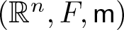 $(\mathbb{R}^n,F,\mathsf{m})$, where $F\colon \mathbb{R}^n\times \mathbb{R}^n\to [0,\infty)$ is defined by
 \begin{equation}
F(x,y)=|y|-\frac{\langle x,y\rangle\theta}{|x|},\quad\text{if } x\ne O\quad\text{and}\quad F(O,y)=|y|,
\end{equation}
\begin{equation}
F(x,y)=|y|-\frac{\langle x,y\rangle\theta}{|x|},\quad\text{if } x\ne O\quad\text{and}\quad F(O,y)=|y|,
\end{equation} for some 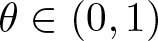 $\theta\in(0,1)$ and $\mathsf{m}$ stands for the Busemann–Hausdorff measure induced by F. Here,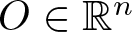 $O\in \mathbb{R}^n$ is the origin, $|\cdot|$ and $\langle\cdot,\cdot \rangle$ denote the norm and the inner product in $\mathbb{R}^n$. The function F is not a Finsler metric, since it is not continuous at the origin. However, it has various remarkable properties (away from O).
On the one hand, since relation (21) holds, theorem 2.3 yields projectively flatness, i.e., all the geodesics are straight (Euclidean) lines. Denote 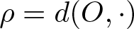 $\rho=d(O,\cdot)$ the Finslerian distance from the origin. Since the geodesics starting from the origin are precisely the integral curves of $\nabla \rho$, it follows that x is parallel with $\nabla\rho$. Using proposition 2.4 and the homogeneity of the flag curvature and the reduced S-curvature we obtain
 \begin{equation}
\mathbf{K}(x,\nabla\rho(x))=\mathbf{K}(x,x)=0\quad\text{and}\quad \overline{\mathbf{S}}(x,\nabla\rho(x))=\overline{\mathbf{S}}(x,x)=0,\quad \forall x\in \mathbb{R}^n, x\ne O,
\end{equation}
\begin{equation}
\mathbf{K}(x,\nabla\rho(x))=\mathbf{K}(x,x)=0\quad\text{and}\quad \overline{\mathbf{S}}(x,\nabla\rho(x))=\overline{\mathbf{S}}(x,x)=0,\quad \forall x\in \mathbb{R}^n, x\ne O,
\end{equation} which precisely means that 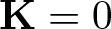 $\mathbf{K}=0$,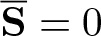 $\overline{\mathbf{S}}=0$ along $\nabla \rho$.
On the other hand, by an easy computation we obtain for every 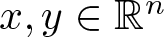 $x,y\in \mathbb{R}^n$ that
 \begin{equation}
\textbf{rev}(x,y)\le \textbf{rev}(x,x)=\frac{1+\theta}{1-\theta}\stackrel{\textrm{def}}{=} \lambda,\quad\text{if }x\ne O,\quad\text{and}\quad \mathbf{rev}(O,y)=1,
\end{equation}
\begin{equation}
\textbf{rev}(x,y)\le \textbf{rev}(x,x)=\frac{1+\theta}{1-\theta}\stackrel{\textrm{def}}{=} \lambda,\quad\text{if }x\ne O,\quad\text{and}\quad \mathbf{rev}(O,y)=1,
\end{equation} hence  $\lambda_F(\mathbb{R}^n)=\lambda\in(1,\infty)$. If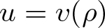 $u=v(\rho)$ is a radially symmetric function with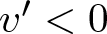 $v' \lt 0$, then one has equality in (31). The latter provides the difference between the two common forms of Hardy inequalities in the Finsler setting, compare e.g., inequalities (2) and (3).
To remedy the discontinuity at the origin, one could simply puncture the space (considering only  $\mathbb{R}^n\setminus\{O\}$), which results in a loss of computational convenience: By construction, the distance from O is easier to compute than the distance from any other base point. An other option (what is chosen here) is to ‘smooth out’ the jump at the origin, which can be done by a careful approximation of F, partially retaining the aforementioned favourable properties. We have the following result.
Theorem 4.1. Let 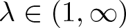 $\lambda\in (1,\infty)$ and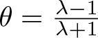 $\theta=\frac{\lambda-1}{\lambda+1}$. Construct the family $\mathcal{F}_{0,0,\lambda}=\{(\mathbb{R}^n,F_\varepsilon,\mathsf{m}_\varepsilon)\}_{\varepsilon \gt 0}$ of FMMMs, where $F_\varepsilon\colon T\mathbb{R}^n\simeq\mathbb{R}^n\times\mathbb{R}^n\to [0,\infty)$ is defined by
 \begin{equation}
F_\varepsilon(x,y)=|y|-\frac{\langle x,y\rangle(|x|+2\varepsilon)\theta}{(|x|+\varepsilon)^2},
\end{equation}
\begin{equation}
F_\varepsilon(x,y)=|y|-\frac{\langle x,y\rangle(|x|+2\varepsilon)\theta}{(|x|+\varepsilon)^2},
\end{equation} and  $\mathsf{m}_\varepsilon$ is the Busemann–Hausdorff measure induced by Fɛ. The following statements hold:
(i) For every ɛ > 0, the triple
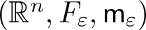
$(\mathbb{R}^n, F_\varepsilon,\mathsf{m}_\varepsilon)$ is an FMMM. In addition, Fɛ is a projectively flat Randers metric, with reversibility
$\lambda_{F_\varepsilon}(\mathbb{R}^n)=\lambda$.(ii) For every
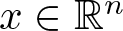
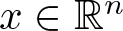
$x\in \mathbb{R}^n$ with
$x\ne 0$ one has
\begin{equation*}
\mathbf{K}_\varepsilon(x,x)\to 0,\quad \overline{\mathbf{S}}_\varepsilon(x,x)\to 0,\quad\mbox{and}\quad \mathbf{rev}_\varepsilon(x,x)\to\lambda,\quad\text{as}\quad \varepsilon\to 0.
\end{equation*}(iii) For every ɛ > 0 and
$x\in \mathbb{R}^n$, one has
\begin{equation*}
\mathbf{K}_\varepsilon(x,x)\le 0,\quad \overline{\mathbf{S}}_\varepsilon(x,x)\le 0,\quad\mbox{and}\quad
\mathbf{rev}_\varepsilon(x,x)\le\lambda.
\end{equation*}




Proof. Denote 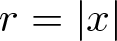 $r=|x|$. Using the standard notation of Randers metrics (see §2.3) we have
 \begin{equation*}
F_\varepsilon(x,y)=\sqrt{a_{ij}(x)y^iy^j}+b_i(x)y^i,\quad\mbox{where}\quad a_{ij}(x)=\delta_{ij}\quad\mbox{and}\quad b_i(x)=-\frac{x^i(r+2\varepsilon)\theta}{(r+\varepsilon)^2},
\end{equation*}
\begin{equation*}
F_\varepsilon(x,y)=\sqrt{a_{ij}(x)y^iy^j}+b_i(x)y^i,\quad\mbox{where}\quad a_{ij}(x)=\delta_{ij}\quad\mbox{and}\quad b_i(x)=-\frac{x^i(r+2\varepsilon)\theta}{(r+\varepsilon)^2},
\end{equation*} while δij is the Kronecker delta (see (24)). Since  $a^{ij}(x)=\{a_{ij}(x)\}^{-1}=\delta_{ij}$, we have
 \begin{equation*}\|b(x)\|_a = \sqrt{a^{ij}(x)b_i(x)b_j(x)}=\frac{r(r+2\varepsilon)\theta}{(r+\varepsilon)^2} \lt \theta \lt 1.\end{equation*}
 Obviously Fɛ is smooth, hence it is a Randers metric on  $\mathbb{R}^n$. In addition, according to remark 2.5, the metric Fɛ is projectively flat. Indeed, the Euclidean metric is projectively flat, and one has
 \begin{equation*}
b_i\,\mathrm{d} x^i=D\beta(x),\quad\mbox{where}\quad \beta(x)=-\left(r+\frac{\varepsilon^2}{r+\varepsilon}\right)\theta.
\end{equation*}
\begin{equation*}
b_i\,\mathrm{d} x^i=D\beta(x),\quad\mbox{where}\quad \beta(x)=-\left(r+\frac{\varepsilon^2}{r+\varepsilon}\right)\theta.
\end{equation*} Let 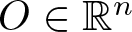 $O\in \mathbb{R}^n$ be the origin. For $\rho_\varepsilon(x)=d(O,x)$ and $\overleftarrow{\rho_\varepsilon} (x)=d(x,O)$ we obtain:
 \begin{equation*}
\rho_\varepsilon(x)=r\cdot \frac{r(1-\theta)+ \varepsilon }{r+\varepsilon}\quad\mbox{and}\quad
\overleftarrow{\rho_\varepsilon} (x) =r\cdot \frac{r(1+\theta)+ \varepsilon }{r+\varepsilon}.
\end{equation*}
\begin{equation*}
\rho_\varepsilon(x)=r\cdot \frac{r(1-\theta)+ \varepsilon }{r+\varepsilon}\quad\mbox{and}\quad
\overleftarrow{\rho_\varepsilon} (x) =r\cdot \frac{r(1+\theta)+ \varepsilon }{r+\varepsilon}.
\end{equation*}In addition, one has
 \begin{equation}
D\rho_\varepsilon(x)=\left(\frac{1}{r}-\frac{ (r+2 \varepsilon )\theta}{(r+\varepsilon )^2}\right)\cdot x\quad\mbox{and}\quad\nabla\rho_\varepsilon(x)=\frac{(r+\varepsilon)^2}{r(r+\varepsilon)^2-r^2(r+2\varepsilon)\theta}\cdot x.
\end{equation}
\begin{equation}
D\rho_\varepsilon(x)=\left(\frac{1}{r}-\frac{ (r+2 \varepsilon )\theta}{(r+\varepsilon )^2}\right)\cdot x\quad\mbox{and}\quad\nabla\rho_\varepsilon(x)=\frac{(r+\varepsilon)^2}{r(r+\varepsilon)^2-r^2(r+2\varepsilon)\theta}\cdot x.
\end{equation} According to relation (23), the density of the Busemann–Hausdorff measure  $\mathsf{m}_\varepsilon$ induced by Fɛ is
 \begin{equation*}
\sigma_{F_\varepsilon}(x)=\left(1-\frac{r^2 (r+2 \varepsilon)^2\theta^2}{(r+\varepsilon)^4}\right)^\frac{n+1}{2}.
\end{equation*}
\begin{equation*}
\sigma_{F_\varepsilon}(x)=\left(1-\frac{r^2 (r+2 \varepsilon)^2\theta^2}{(r+\varepsilon)^4}\right)^\frac{n+1}{2}.
\end{equation*} By proposition 2.4, for every ɛ > 0 and 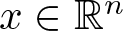 $x\in \mathbb{R}^n$ we obtain
 \begin{align*}
\mathbf{K}_{\rho_\varepsilon}(r)
& \stackrel{\textrm{def}}{=}\mathbf{K}_\varepsilon(x,x)=-\frac{3 \varepsilon ^2 (r+\varepsilon)^4 \theta (1-\theta)}{\left((r+\varepsilon)^2- r (r+2 \varepsilon)\theta \right)^4}\le 0, \\
\overline{\mathbf{S}}_{\rho_\varepsilon}(r)
& \stackrel{\textrm{def}}{=}
\overline{\mathbf{S}}_\varepsilon(x,x)=-\frac{(n+1)\varepsilon ^2(r+\varepsilon ) \theta }{\left(r+\varepsilon \right)^4- r^2 \left(r+2 \varepsilon\right)^2\theta^2}\le 0, \\
\mathbf{rev}_{\rho_\varepsilon}(r)
& \stackrel{\textrm{def}}{=}\mathbf{rev}_\varepsilon(x,x)=\frac{1+\|b(x)\|_a}{1-\|b(x)\|_a}=\frac{1+\frac{r(r+2\varepsilon)\theta}{(r+\varepsilon)^2}}{1-\frac{r(r+2\varepsilon)\theta}{(r+\varepsilon)^2}}\le \frac{1+\theta}{1-\theta}=\lambda.
\end{align*}
\begin{align*}
\mathbf{K}_{\rho_\varepsilon}(r)
& \stackrel{\textrm{def}}{=}\mathbf{K}_\varepsilon(x,x)=-\frac{3 \varepsilon ^2 (r+\varepsilon)^4 \theta (1-\theta)}{\left((r+\varepsilon)^2- r (r+2 \varepsilon)\theta \right)^4}\le 0, \\
\overline{\mathbf{S}}_{\rho_\varepsilon}(r)
& \stackrel{\textrm{def}}{=}
\overline{\mathbf{S}}_\varepsilon(x,x)=-\frac{(n+1)\varepsilon ^2(r+\varepsilon ) \theta }{\left(r+\varepsilon \right)^4- r^2 \left(r+2 \varepsilon\right)^2\theta^2}\le 0, \\
\mathbf{rev}_{\rho_\varepsilon}(r)
& \stackrel{\textrm{def}}{=}\mathbf{rev}_\varepsilon(x,x)=\frac{1+\|b(x)\|_a}{1-\|b(x)\|_a}=\frac{1+\frac{r(r+2\varepsilon)\theta}{(r+\varepsilon)^2}}{1-\frac{r(r+2\varepsilon)\theta}{(r+\varepsilon)^2}}\le \frac{1+\theta}{1-\theta}=\lambda.
\end{align*}Considering the limit cases of the above inequalities, we obtain
 \begin{equation*}
\lim_{r\to\infty}\mathbf{K}_{\rho_\varepsilon}(r)=0,\quad
\lim_{r\to\infty}\overline{\mathbf{S}}_{\rho_\varepsilon}(r)=0,\quad
\lim_{r\to\infty}\mathbf{rev}_{\rho_\varepsilon}(r)=\lambda,\quad \forall \varepsilon \gt 0,
\end{equation*}
\begin{equation*}
\lim_{r\to\infty}\mathbf{K}_{\rho_\varepsilon}(r)=0,\quad
\lim_{r\to\infty}\overline{\mathbf{S}}_{\rho_\varepsilon}(r)=0,\quad
\lim_{r\to\infty}\mathbf{rev}_{\rho_\varepsilon}(r)=\lambda,\quad \forall \varepsilon \gt 0,
\end{equation*}and
 \begin{equation*}
\lim_{\varepsilon\to0}\mathbf{K}_{\rho_\varepsilon}(r)=0,\quad
\lim_{\varepsilon\to0}\overline{\mathbf{S}}_{\rho_\varepsilon}(r)=0,\quad \lim_{\varepsilon\to0}\mathbf{rev}_{\rho_\varepsilon}(r)=\lambda,\quad \forall r \gt 0.
\end{equation*}
\begin{equation*}
\lim_{\varepsilon\to0}\mathbf{K}_{\rho_\varepsilon}(r)=0,\quad
\lim_{\varepsilon\to0}\overline{\mathbf{S}}_{\rho_\varepsilon}(r)=0,\quad \lim_{\varepsilon\to0}\mathbf{rev}_{\rho_\varepsilon}(r)=\lambda,\quad \forall r \gt 0.
\end{equation*} Moreover, for every ɛ > 0 and 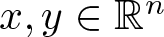 $x,y\in \mathbb{R}^n$ one has
 \begin{align}
\mathbf{rev}_\varepsilon(x,y)&=\frac{F_\varepsilon(x,-y)}{F_\varepsilon(x,y)}\le \frac{F_\varepsilon(x,-x)}{F_\varepsilon(x,x)}\\ & \nonumber =\mathbf{rev}_\varepsilon(x,x)\le \lambda,\quad\text{if }x\ne O\quad\text{and}\quad
\mathbf{rev}_\varepsilon(O,y)=1,
\end{align}
\begin{align}
\mathbf{rev}_\varepsilon(x,y)&=\frac{F_\varepsilon(x,-y)}{F_\varepsilon(x,y)}\le \frac{F_\varepsilon(x,-x)}{F_\varepsilon(x,x)}\\ & \nonumber =\mathbf{rev}_\varepsilon(x,x)\le \lambda,\quad\text{if }x\ne O\quad\text{and}\quad
\mathbf{rev}_\varepsilon(O,y)=1,
\end{align} thus, on also has  $\lambda_{F_\varepsilon}(\mathbb{R}^n)=\lambda$, for every ɛ > 0.
We make the following observations.
(a) The above construction can be motivated as follows. First, Randers-type metrics are often considered as a first step towards Finsler geometry from Riemannian geometry, it is quite natural to consider them in this case as well. Second, every radially symmetric Randers metric with respect to some x 0, needs to have
$\mathbf{rev}(x_0,\cdot)=1$ (as in (39)), otherwise it would be discontinuous at x 0. Since our F in (34) has constant
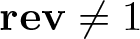
$\mathbf{rev}\ne 1$ along
$\nabla \rho$, some smoothing/perturbation is unavoidable at x 0. Indeed, one can consider other perturbations instead of the one in (37). The latter is chosen due to its simplicity and computational convenience.(b) One can consider a measure
$\mathsf{m}_\varepsilon$ with density
$\sigma_\varepsilon=\sigma_F\cdot e^{-s\rho_\varepsilon}$, to obtain
\begin{equation*}
\sup_{x\in \mathbb{R}^n}\overline{\mathbf{S}}_\varepsilon(x,x)\le s\quad\mbox{and}\quad \lim_{\varepsilon\to 0} \overline{\mathbf{S}}_\varepsilon(x,x)=s,\quad \forall x\in \mathbb{R}^n\setminus\{x_0\}.
\end{equation*}In this section we only need s = 0. This observation, however, is exploited in §5.
(c) We note that in case of the reduced S-curvature,
$\overline{\mathbf{S}}\le0$ holds also globally. Surprisingly, in case of the flag curvature,
$\mathbf{K}\le 0$ is not a global property. For example, one has
\begin{equation*}
\mathbf{K}_\varepsilon(x,-x)=\frac{3 \varepsilon ^2 (r+\varepsilon)^4 \theta (1+\theta)}{\left((r+\varepsilon)^2+ r (r+2 \varepsilon)\theta \right)^4} \gt 0,\quad \forall x\in \mathbb{R}^n.
\end{equation*}(d) Observe that
$\max\{F^{*}_\varepsilon(\pm D\rho_\varepsilon)\}=F^{*}_\varepsilon(D\rho_\varepsilon)=1$. Indeed, relation (10) implies
$F^*_\varepsilon(D\rho_\varepsilon)=1$, and one has
\begin{equation*}
F^*_\varepsilon(-D\rho_\varepsilon)=\frac{1-\frac{r(r+2\varepsilon)}{(r+\varepsilon)^2}\theta}{1+\frac{r(r+2\varepsilon)}{(r+\varepsilon)^2}\theta}\stackrel{\textrm{def}}{=} h_\varepsilon(r),\quad\mbox{where}\quad \frac{1-\theta}{1+\theta}\le h_\varepsilon(r)\le1.
\end{equation*}Note that
$F^*_\varepsilon$ can be computed as in Shen [Reference Shen12, Example 3.1.1], while
$D\rho_\varepsilon$ is given by relation (38).










4.2. Sufficient conditions for sharpness
In this section, we present sufficient conditions for the sharpness of Hardy inequalities provided by Riccati pairs on the spaces of 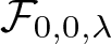 $\mathcal{F}_{0,0,\lambda}$, introduced in theorem 4.1.
Let  $(\mathbb{R}^n,F_\varepsilon,\mathsf{m}_\varepsilon)\in\mathcal{F}_{0,0,\lambda}$ for some ɛ > 0 and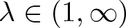 $\lambda\in(1,\infty)$. Then for every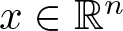 $x\in \mathbb{R}^n$, one has
 \begin{equation*}
\mathbf{K}_\varepsilon(x,x)\le 0,\quad \overline{\mathbf{S}}_\varepsilon(x,x)\le 0,\quad\mbox{and}\quad
\mathbf{rev}_\varepsilon(x,x)\le\lambda=\lambda_{F_\varepsilon}(\mathbb{R}^n).
\end{equation*}
\begin{equation*}
\mathbf{K}_\varepsilon(x,x)\le 0,\quad \overline{\mathbf{S}}_\varepsilon(x,x)\le 0,\quad\mbox{and}\quad
\mathbf{rev}_\varepsilon(x,x)\le\lambda=\lambda_{F_\varepsilon}(\mathbb{R}^n).
\end{equation*} Denote 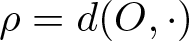 $\rho=d(O,\cdot)$ the distance from the origin. The Laplace comparison theorem (see theorem 2.2) implies
 \begin{equation*}
\Delta_{F_\varepsilon}(\rho_\varepsilon)\ge \frac{n-1}{\rho_\varepsilon}\stackrel{\textrm{def}}{=} L^{0,0}(\rho_\varepsilon).
\end{equation*}
\begin{equation*}
\Delta_{F_\varepsilon}(\rho_\varepsilon)\ge \frac{n-1}{\rho_\varepsilon}\stackrel{\textrm{def}}{=} L^{0,0}(\rho_\varepsilon).
\end{equation*} Let  $R\in(0,+\infty]$, $L(t)\le L^{0,0}(t)$ for every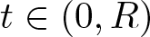 $t\in(0,R)$, and define
 \begin{equation*}\Omega_\varepsilon=\{x\in \mathbb{R}^n : \rho_\varepsilon(x) \lt R\}.\end{equation*}
 Suppose that (L, W) is a 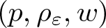 $(p,\rho_\varepsilon,w)$-Riccati pair in $(0,R)$, that is $W\colon(0,R)\to (0,\infty)$ is continuous, $w\colon(0,R)\to (0,\infty)$ is of class C 1, and there exists $G\colon(0,R)\to(0,\infty)$ of class C 1 such that
 \begin{equation}
(G(t)w(t))'+G(t)w(t)L(t)-(p-1)G(t)^{p'}w(t)\geq W(t)w(t), \quad\forall t\in (0,R).
\end{equation}
\begin{equation}
(G(t)w(t))'+G(t)w(t)L(t)-(p-1)G(t)^{p'}w(t)\geq W(t)w(t), \quad\forall t\in (0,R).
\end{equation} Then by theorem 3.1, for every  $u\in C_0^\infty(\Omega_\varepsilon)$ one has:
 \begin{align}
\lambda^p\int_{\Omega_\varepsilon} w(\rho_\varepsilon) F^*_\varepsilon(Du)^p\,\mathrm{d} \mathsf{m}_\varepsilon & \ge\int_{\Omega_\varepsilon} w(\rho_\varepsilon) W(\rho_\varepsilon) |u|^p\,\mathrm{d} \mathsf{m}_\varepsilon.
\end{align}
\begin{align}
\lambda^p\int_{\Omega_\varepsilon} w(\rho_\varepsilon) F^*_\varepsilon(Du)^p\,\mathrm{d} \mathsf{m}_\varepsilon & \ge\int_{\Omega_\varepsilon} w(\rho_\varepsilon) W(\rho_\varepsilon) |u|^p\,\mathrm{d} \mathsf{m}_\varepsilon.
\end{align} As in remark 3.2(e), suppose that a function G > 0 verifies the Riccati ODI (40) with equality, and define  $v\colon (0,R)\to\mathbb{R}$ by
 \begin{equation}
-(\log v(t))'=-\frac{v'(t)}{v(t)}=G(t)^\frac{1}{p-1}.
\end{equation}
\begin{equation}
-(\log v(t))'=-\frac{v'(t)}{v(t)}=G(t)^\frac{1}{p-1}.
\end{equation}Since G is smooth and positive, it follows that v is smooth, positive, and decreasing. Introduce the notation
 \begin{equation}
\mathcal{I}(f;a,b)=\int_a^b f(t)t^{n-1}\,\mathrm{d} t,
\end{equation}
\begin{equation}
\mathcal{I}(f;a,b)=\int_a^b f(t)t^{n-1}\,\mathrm{d} t,
\end{equation} for arbitrary continuous functions  $f\colon[a,b]\to\mathbb{R}$, with $0 \lt a \lt b \lt R$.
We have the following result.
Theorem 4.3. Fix 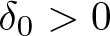 $\delta_0 \gt 0$ and let $t_1=t_1(\delta),t_2=t_2(\delta),t_3=t_3(\delta),t_4=t_4(\delta)$ be continuous functions admitting a (possibly infinite) limit at infinity, such that for every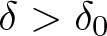 $\delta \gt \delta_0$ one has $0 \lt t_1 \lt t_2 \lt t_3 \lt t_4 \lt R$. Suppose that the following limits hold true:
 \begin{align*}
\lim_{\delta\to\infty} l_0(\delta) & =0,\quad\mbox{where}\\ &\quad l_0(\delta)\stackrel {\textrm {def}} {=} \frac{v(t_2)^p\cdot \mathcal{I}(w;t_1,t_2)}{(t_2-t_1)^p\cdot \mathcal{I}(wWv^p;t_2,t_3)}+ \frac{v(t_3)^p\cdot \mathcal{I}(w;t_3,t_4)}{(t_4-t_3)^p\cdot \mathcal{I}(wWv^p;t_2,t_3)}, \\
\lim_{\delta\to\infty} l_1(\delta) & =1,\quad\mbox{where}\quad l_1(\delta)\stackrel{\textrm{def}}{=}\max_{t\in [t_2,t_3]} \frac{G(t)^{p'}}{W(t)}.
\end{align*}
\begin{align*}
\lim_{\delta\to\infty} l_0(\delta) & =0,\quad\mbox{where}\\ &\quad l_0(\delta)\stackrel {\textrm {def}} {=} \frac{v(t_2)^p\cdot \mathcal{I}(w;t_1,t_2)}{(t_2-t_1)^p\cdot \mathcal{I}(wWv^p;t_2,t_3)}+ \frac{v(t_3)^p\cdot \mathcal{I}(w;t_3,t_4)}{(t_4-t_3)^p\cdot \mathcal{I}(wWv^p;t_2,t_3)}, \\
\lim_{\delta\to\infty} l_1(\delta) & =1,\quad\mbox{where}\quad l_1(\delta)\stackrel{\textrm{def}}{=}\max_{t\in [t_2,t_3]} \frac{G(t)^{p'}}{W(t)}.
\end{align*} Then inequality (41) is sharp on 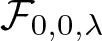 $\mathcal{F}_{0,0,\lambda}$, in the sense that it no longer holds on each FMMM of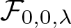 $\mathcal{F}_{0,0,\lambda}$ if we multiply its right-hand side by a constant c > 1.
Proof. Let ɛ > 0 and define the limit function  $u^\star_\varepsilon\colon \Omega\to (0,\infty)$ of inequality (41) by
 \begin{equation*}u^\star_\varepsilon(x)=v(\rho_\varepsilon(x)).\end{equation*}
 Denote  $T=(t_1,t_2,t_3,t_4)$ and construct
 \begin{equation*}u^\star_{\varepsilon,T}=v_T(\rho_\varepsilon),\end{equation*}
where the function vT and its derivative satisfy
 \begin{align}
v_T(t)=\begin{cases}
0, & \mbox{if }0 \lt t\le t_1, \\
v(t_2)\frac{t-t_1}{t_2-t_1}, & \mbox{if }t_1\le t\le t_2, \\
v(t), & \mbox{if }t_2\le t\le t_3, \\
v(t_3)\frac{t_4-t}{t_4-t_3}, & \mbox{if }t_3\le t\le t_4, \\
0, & \mbox{if }t_4\le t \lt R,
\end{cases}\quad\mbox{and}\quad v_T'(t)=\begin{cases}
0, & \mbox{if }0 \lt t \lt t_1, \\
\frac{v(t_2)}{t_2-t_1}, & \mbox{if }t_1 \lt t \lt t_2, \\
v'(t), & \mbox{if }t_2 \lt t \lt t_3, \\
-\frac{v(t_3)}{t_4-t_3}, & \mbox{if }t_3 \lt t \lt t_4, \\
0, & \mbox{if }t_4 \lt t \lt R.
\end{cases}
\end{align}
\begin{align}
v_T(t)=\begin{cases}
0, & \mbox{if }0 \lt t\le t_1, \\
v(t_2)\frac{t-t_1}{t_2-t_1}, & \mbox{if }t_1\le t\le t_2, \\
v(t), & \mbox{if }t_2\le t\le t_3, \\
v(t_3)\frac{t_4-t}{t_4-t_3}, & \mbox{if }t_3\le t\le t_4, \\
0, & \mbox{if }t_4\le t \lt R,
\end{cases}\quad\mbox{and}\quad v_T'(t)=\begin{cases}
0, & \mbox{if }0 \lt t \lt t_1, \\
\frac{v(t_2)}{t_2-t_1}, & \mbox{if }t_1 \lt t \lt t_2, \\
v'(t), & \mbox{if }t_2 \lt t \lt t_3, \\
-\frac{v(t_3)}{t_4-t_3}, & \mbox{if }t_3 \lt t \lt t_4, \\
0, & \mbox{if }t_4 \lt t \lt R.
\end{cases}
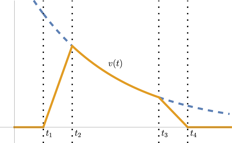
\end{align} Note that  $v'_T$ is not defined in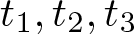 $t_1,t_2,t_3$ and t 4. In addition, both vT and $v'_T$ are supported in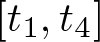 $[t_1,t_4]$. For a schematic illustration of vT we refer to figure 1.
Illustration of the ‘tent-like’ function  $v_T(t)$: coincides with v(t) on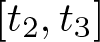 $[t_2,t_3]$, linearized on both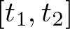 $[t_1,t_2]$ and $[t_3,t_4]$, and zero elsewhere.
To prove the sharpness of inequality (41), we show that under a suitable limiting procedure, one has
 \begin{equation*}
\frac{\lambda^p\displaystyle\int_{\Omega_\varepsilon} w(\rho_\varepsilon) F^*_\varepsilon(Du^\star_{\varepsilon,T})^p\,\mathrm{d} \mathsf{m}_\varepsilon}{
\displaystyle\int_{\Omega_\varepsilon} w(\rho_\varepsilon) W(\rho_\varepsilon) (u_{\varepsilon,T}^\star)^p\,\mathrm{d} \mathsf{m}_\varepsilon}\to 1.
\end{equation*}
\begin{equation*}
\frac{\lambda^p\displaystyle\int_{\Omega_\varepsilon} w(\rho_\varepsilon) F^*_\varepsilon(Du^\star_{\varepsilon,T})^p\,\mathrm{d} \mathsf{m}_\varepsilon}{
\displaystyle\int_{\Omega_\varepsilon} w(\rho_\varepsilon) W(\rho_\varepsilon) (u_{\varepsilon,T}^\star)^p\,\mathrm{d} \mathsf{m}_\varepsilon}\to 1.
\end{equation*}As a first step, we use polar transforms to reduce the above integrals to one dimension. We also establish some fine estimates on the distance and the density of the measure.
Using the notations 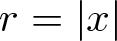 $r=|x|$ and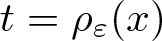 $t=\rho_\varepsilon(x)$, it follows that
 \begin{equation*}t=r\cdot \frac{r(1-\theta)+ \varepsilon }{r+\varepsilon}\quad\iff\quad r=\frac{t-\varepsilon+\sqrt{(t+\varepsilon)^2-4t\varepsilon\theta}}{2(1-\theta)}\stackrel{\textrm{def}}{=} \varphi_\varepsilon(t),\end{equation*}
hence we obtain
 \begin{equation}
\sigma_\varepsilon(r)r^{n-1}\,\mathrm{d} r=\sigma_\varepsilon(\varphi_\varepsilon(t))\varphi_\varepsilon(t)^{n-1}\varphi_\varepsilon'(t)\,\mathrm{d} t\stackrel{\textrm{def}}{=}\psi_\varepsilon(t)\,\mathrm{d} t.
\end{equation}
\begin{equation}
\sigma_\varepsilon(r)r^{n-1}\,\mathrm{d} r=\sigma_\varepsilon(\varphi_\varepsilon(t))\varphi_\varepsilon(t)^{n-1}\varphi_\varepsilon'(t)\,\mathrm{d} t\stackrel{\textrm{def}}{=}\psi_\varepsilon(t)\,\mathrm{d} t.
\end{equation} Since for every 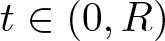 $t\in(0,R)$ one has
 \begin{equation*}
t\le \varphi_\varepsilon(t)\le\frac{t}{1-\theta},\quad 1\le \varphi'_\varepsilon(t)\le \frac{1}{1-\theta},\quad\mbox{and}\quad\left(1-\theta^2\right)^\frac{n+1}{2}\le \sigma_\varepsilon(\varphi_\varepsilon(t))\le 1,
\end{equation*}
\begin{equation*}
t\le \varphi_\varepsilon(t)\le\frac{t}{1-\theta},\quad 1\le \varphi'_\varepsilon(t)\le \frac{1}{1-\theta},\quad\mbox{and}\quad\left(1-\theta^2\right)^\frac{n+1}{2}\le \sigma_\varepsilon(\varphi_\varepsilon(t))\le 1,
\end{equation*}we obtain
 \begin{equation}
ct^{n-1}\stackrel{\textrm{def}}{=}\left(1-\theta^2\right)^\frac{n+1}{2}t^{n-1}\le \psi_\varepsilon(t)\le \frac{t^{n-1}}{(1-\theta)^n}\stackrel{\textrm{def}}{=} Ct^{n-1}.
\end{equation}
\begin{equation}
ct^{n-1}\stackrel{\textrm{def}}{=}\left(1-\theta^2\right)^\frac{n+1}{2}t^{n-1}\le \psi_\varepsilon(t)\le \frac{t^{n-1}}{(1-\theta)^n}\stackrel{\textrm{def}}{=} Ct^{n-1}.
\end{equation}Note that c and C are independent of ɛ.
Since v is positive and decreasing, the positive homogeneity of  $F^*_\varepsilon$ and the relations from (44) imply
 \begin{align}
F^*_\varepsilon(Du^\star_{\varepsilon,T})=F^*_\varepsilon(v_T'(\rho_\varepsilon)D\rho_\varepsilon)=\begin{cases}
\frac{v(t_2)}{t_2-t_1}F^*_\varepsilon(D\rho_\varepsilon), & \text{if } \rho_\varepsilon\in(t_1,t_2), \\
|v'(\rho_\varepsilon)|F^*_\varepsilon(-D\rho_\varepsilon) & \text{if } \rho_\varepsilon\in(t_2,t_3), \\
\frac{v(t_3)}{t_4-t_3}F^*_\varepsilon(-D\rho_\varepsilon) & \text{if } \rho_\varepsilon\in(t_3,t_4), \\
0, & \text{if }\rho_\varepsilon\in(0,t_1)\cup(t_4,R).
\end{cases}
\end{align}
\begin{align}
F^*_\varepsilon(Du^\star_{\varepsilon,T})=F^*_\varepsilon(v_T'(\rho_\varepsilon)D\rho_\varepsilon)=\begin{cases}
\frac{v(t_2)}{t_2-t_1}F^*_\varepsilon(D\rho_\varepsilon), & \text{if } \rho_\varepsilon\in(t_1,t_2), \\
|v'(\rho_\varepsilon)|F^*_\varepsilon(-D\rho_\varepsilon) & \text{if } \rho_\varepsilon\in(t_2,t_3), \\
\frac{v(t_3)}{t_4-t_3}F^*_\varepsilon(-D\rho_\varepsilon) & \text{if } \rho_\varepsilon\in(t_3,t_4), \\
0, & \text{if }\rho_\varepsilon\in(0,t_1)\cup(t_4,R).
\end{cases}
\end{align}According to remark 4.2(d), one has
 \begin{align*}&F^*_\varepsilon(D\rho_\varepsilon)=1,\quad\mbox{and}\quad F^*_\varepsilon(-D\rho_\varepsilon)=\frac{1-\frac{r(r+2\varepsilon)}{(r+\varepsilon)^2}\theta}{1+\frac{r(r+2\varepsilon)}{(r+\varepsilon)^2}\theta}\stackrel{\textrm{def}}{=} h_\varepsilon(r), \\ & \quad\mbox{where}\quad \frac{1-\theta}{1+\theta}\le h_\varepsilon(r)\le1.\end{align*}
 By a simple computation, we obtain that  $h_\varepsilon(r)$ is decreasing in r, increasing in ɛ, and approaches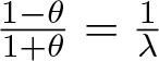 $\frac{1-\theta}{1+\theta}=\frac{1}{\lambda}$ as ɛ → 0. Since $r=\varphi_\varepsilon(t)\ge t$, we also have
 \begin{equation}
h_\varepsilon(\varphi_\varepsilon(t))\le h_\varepsilon(t)\le 1.
\end{equation}
\begin{equation}
h_\varepsilon(\varphi_\varepsilon(t))\le h_\varepsilon(t)\le 1.
\end{equation}In the sequel, denote by ω the volume of the Euclidean unit ball of dimension n.
On the one hand, relations (45) and (47) yield
 \begin{align*}
&I\stackrel{\textrm{def}}{=}\frac{1}{n\omega} \int_{\Omega_\varepsilon} w(\rho_\varepsilon) F^*_\varepsilon(Du^\star_{\varepsilon,T})^p\,\mathrm{d} \mathsf{m}_\varepsilon =\frac{v(t_2)^p}{(t_2-t_1)^p}\int_{t_1}^{t_2} w(t) \psi_\varepsilon(t)\,\mathrm{d} t \\
& \quad + \int_{t_2}^{t_3} w(t)|v'(t)|^p h_\varepsilon^p(\varphi_\varepsilon(t)) \psi_\varepsilon(t)\,\mathrm{d} t
+\frac{v(t_3)^p}{(t_4-t_3)^p}\int_{t_3}^{t_4} w(t) h_\varepsilon^p(\varphi_\varepsilon(t))\psi_\varepsilon(t)\,\mathrm{d} t.
\end{align*}
\begin{align*}
&I\stackrel{\textrm{def}}{=}\frac{1}{n\omega} \int_{\Omega_\varepsilon} w(\rho_\varepsilon) F^*_\varepsilon(Du^\star_{\varepsilon,T})^p\,\mathrm{d} \mathsf{m}_\varepsilon =\frac{v(t_2)^p}{(t_2-t_1)^p}\int_{t_1}^{t_2} w(t) \psi_\varepsilon(t)\,\mathrm{d} t \\
& \quad + \int_{t_2}^{t_3} w(t)|v'(t)|^p h_\varepsilon^p(\varphi_\varepsilon(t)) \psi_\varepsilon(t)\,\mathrm{d} t
+\frac{v(t_3)^p}{(t_4-t_3)^p}\int_{t_3}^{t_4} w(t) h_\varepsilon^p(\varphi_\varepsilon(t))\psi_\varepsilon(t)\,\mathrm{d} t.
\end{align*} Applying relations (46) and (48), and using the definition of  $\mathcal{I}$ from (43), it follows that
 \begin{align*}
I & \le \frac{v(t_2)^p}{(t_2-t_1)^p}\int_{t_1}^{t_2} w(t) \psi_\varepsilon(t)\,\mathrm{d} t+ \int_{t_2}^{t_3} w(t)|v'(t)|^p h_\varepsilon^p(t) \psi_\varepsilon(t)\,\mathrm{d} t +\frac{v(t_3)^p}{(t_4-t_3)^p}\\ & \quad \times \int_{t_3}^{t_4} w(t) h_\varepsilon^p(t)\psi_\varepsilon(t)\,\mathrm{d} t
\le \frac{Cv(t_2)^p}{(t_2-t_1)^p}\int_{t_1}^{t_2} w(t) t^{n-1}\,\mathrm{d} t+ h_\varepsilon^p(t_2)\int_{t_2}^{t_3} w(t)|v'(t)|^p \psi_\varepsilon(t)\,\mathrm{d} t \\
& \quad +\frac{C h_\varepsilon^p(t_3)v(t_3)^p}{(t_4-t_3)^p}\int_{t_3}^{t_4} w(t)t^{n-1}\,\mathrm{d} t =\frac{Cv(t_2)^p\cdot \mathcal{I}(w;t_1,t_2)}{(t_2-t_1)^p}+ h_\varepsilon^p(t_2)\\
&\quad \times \int_{t_2}^{t_3} w(t)|v'(t)|^p \psi_\varepsilon(t)\,\mathrm{d} t +\frac{C v(t_3)^p\cdot\mathcal{I}(w;t_3,t_4)}{(t_4-t_3)^p}.
\end{align*}
\begin{align*}
I & \le \frac{v(t_2)^p}{(t_2-t_1)^p}\int_{t_1}^{t_2} w(t) \psi_\varepsilon(t)\,\mathrm{d} t+ \int_{t_2}^{t_3} w(t)|v'(t)|^p h_\varepsilon^p(t) \psi_\varepsilon(t)\,\mathrm{d} t +\frac{v(t_3)^p}{(t_4-t_3)^p}\\ & \quad \times \int_{t_3}^{t_4} w(t) h_\varepsilon^p(t)\psi_\varepsilon(t)\,\mathrm{d} t
\le \frac{Cv(t_2)^p}{(t_2-t_1)^p}\int_{t_1}^{t_2} w(t) t^{n-1}\,\mathrm{d} t+ h_\varepsilon^p(t_2)\int_{t_2}^{t_3} w(t)|v'(t)|^p \psi_\varepsilon(t)\,\mathrm{d} t \\
& \quad +\frac{C h_\varepsilon^p(t_3)v(t_3)^p}{(t_4-t_3)^p}\int_{t_3}^{t_4} w(t)t^{n-1}\,\mathrm{d} t =\frac{Cv(t_2)^p\cdot \mathcal{I}(w;t_1,t_2)}{(t_2-t_1)^p}+ h_\varepsilon^p(t_2)\\
&\quad \times \int_{t_2}^{t_3} w(t)|v'(t)|^p \psi_\varepsilon(t)\,\mathrm{d} t +\frac{C v(t_3)^p\cdot\mathcal{I}(w;t_3,t_4)}{(t_4-t_3)^p}.
\end{align*} By relation (42), for every 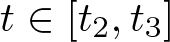 $t\in[t_2,t_3]$ one has
 \begin{equation*}
\frac{1}{W(t)}\left|\frac{v'(t)}{v(t)}\right|^p=\frac{1}{W(t)}\left(-\frac{v'(t)}{v(t)}\right)^p=\frac{G(t)^{p'}}{W(t)}.
\end{equation*}
\begin{equation*}
\frac{1}{W(t)}\left|\frac{v'(t)}{v(t)}\right|^p=\frac{1}{W(t)}\left(-\frac{v'(t)}{v(t)}\right)^p=\frac{G(t)^{p'}}{W(t)}.
\end{equation*} The above function is continuous; thus, it attains its maximum on 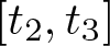 $[t_2,t_3]$. Hence, we have
 \begin{align*}
\int_{t_2}^{t_3} w(t)|v'(t)|^p \psi_\varepsilon(t)\,\mathrm{d} t&=\int_{t_2}^{t_3} \frac{1}{W(t)}\left|\frac{v'(t)}{v(t)}\right|^p w(t) W(t)|v(t)|^p \psi_\varepsilon(t)\,\mathrm{d} t\\
&\le \max_{t\in[t_2,t_3]} \frac{G(t)^{p'}}{W(t)}\cdot \int_{t_2}^{t_3} w(t) W(t) (v(t))^p \psi_\varepsilon(t)\,\mathrm{d} t.
\end{align*}
\begin{align*}
\int_{t_2}^{t_3} w(t)|v'(t)|^p \psi_\varepsilon(t)\,\mathrm{d} t&=\int_{t_2}^{t_3} \frac{1}{W(t)}\left|\frac{v'(t)}{v(t)}\right|^p w(t) W(t)|v(t)|^p \psi_\varepsilon(t)\,\mathrm{d} t\\
&\le \max_{t\in[t_2,t_3]} \frac{G(t)^{p'}}{W(t)}\cdot \int_{t_2}^{t_3} w(t) W(t) (v(t))^p \psi_\varepsilon(t)\,\mathrm{d} t.
\end{align*}On the other hand, we obtain
 \begin{align*}
\nonumber J&\stackrel{\textrm{def}}{=}
\frac{1}{n\omega}
\displaystyle\int_{\Omega_\varepsilon} w(\rho_\varepsilon) W(\rho_\varepsilon) (u_{\varepsilon,T}^\star)^p\,\mathrm{d} \mathsf{m}_\varepsilon=\int_{0}^{R} w(t) W(t) (v_T(t))^p \psi_\varepsilon(t)\,\mathrm{d} t
\end{align*}
\begin{align*}
\nonumber J&\stackrel{\textrm{def}}{=}
\frac{1}{n\omega}
\displaystyle\int_{\Omega_\varepsilon} w(\rho_\varepsilon) W(\rho_\varepsilon) (u_{\varepsilon,T}^\star)^p\,\mathrm{d} \mathsf{m}_\varepsilon=\int_{0}^{R} w(t) W(t) (v_T(t))^p \psi_\varepsilon(t)\,\mathrm{d} t
\end{align*} \begin{align} &\,\ge \int_{t_2}^{t_3} w(t) W(t) (v(t))^p \psi_\varepsilon(t)\,\mathrm{d} t\ge c\cdot \mathcal{I}(wWv^p;t_2,t_3).
\end{align}
\begin{align} &\,\ge \int_{t_2}^{t_3} w(t) W(t) (v(t))^p \psi_\varepsilon(t)\,\mathrm{d} t\ge c\cdot \mathcal{I}(wWv^p;t_2,t_3).
\end{align}Combining the above results and using both estimates of (49), it follows that
 \begin{align*}
\frac{\lambda^p I}{J}
& \le \lambda^p h_\varepsilon^p(t_2)\cdot \max_{t\in[t_2,t_3]} \frac{G(t)^{p'}}{W(t)}+\frac{\lambda^p C}{c}\left(\frac{v(t_2)^p\cdot \mathcal{I}(w;t_1,t_2)}{(t_2-t_1)^p\cdot \mathcal{I}(wWv^p;t_2,t_3)}\right. \nonumber\\ & \left. \quad +\frac{v(t_3)^p\cdot \mathcal{I}(w;t_3,t_4)}{(t_4-t_3)^p\cdot \mathcal{I}(wWv^p;t_2,t_3)}\right) \\
& =\lambda^p h_\varepsilon^p(t_2) l_1(\delta)+\frac{\lambda^p C}{c}l_0(\delta).
\end{align*}
\begin{align*}
\frac{\lambda^p I}{J}
& \le \lambda^p h_\varepsilon^p(t_2)\cdot \max_{t\in[t_2,t_3]} \frac{G(t)^{p'}}{W(t)}+\frac{\lambda^p C}{c}\left(\frac{v(t_2)^p\cdot \mathcal{I}(w;t_1,t_2)}{(t_2-t_1)^p\cdot \mathcal{I}(wWv^p;t_2,t_3)}\right. \nonumber\\ & \left. \quad +\frac{v(t_3)^p\cdot \mathcal{I}(w;t_3,t_4)}{(t_4-t_3)^p\cdot \mathcal{I}(wWv^p;t_2,t_3)}\right) \\
& =\lambda^p h_\varepsilon^p(t_2) l_1(\delta)+\frac{\lambda^p C}{c}l_0(\delta).
\end{align*} Observe that the above inequality holds for every ɛ > 0 and 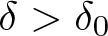 $\delta \gt \delta_0$, in addition, δ, $T=(t_1,t_2,t_3,t_3)$, c, C, λ, l 0, and l 1 are independent of ɛ. To prove the sharpness of (41), it is enough to choose for every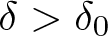 $\delta \gt \delta_0$ an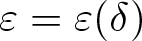 $\varepsilon=\varepsilon(\delta)$ such that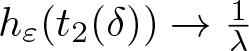 $h_{\varepsilon}(t_2(\delta))\to\frac{1}{\lambda}$ as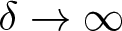 $\delta\to\infty$. Indeed, in this case, since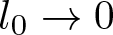 $l_0\to0$ and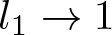 $l_1\to1$ as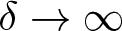 $\delta\to\infty$ we obtain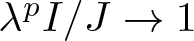 $\lambda^pI/J\to1$ as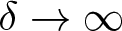 $\delta\to \infty$.
By assumption there exists
 \begin{equation*}\lim_{\delta\to\infty} t_2(\delta)\stackrel{\textrm{def}}{=} l\in[0,R].\end{equation*}
 We distinguish two cases: If l > 0, then choose 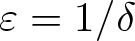 $\varepsilon=1/\delta$, to obtain
 \begin{equation*}
\lim_{\delta\to \infty} h_{\varepsilon}(t_2(\delta))= \lim_{\delta\to \infty}\frac{1-\frac{t_2(\delta)(t_2(\delta)+2/\delta)}{(t_2(\delta)+1/\delta)^2}\theta}{1+\frac{t_2(\delta)(t_2(\delta)+2/\delta)}{(t_2(\delta)+1/\delta)^2}\theta}=\frac{1-\theta}{1+\theta}=\frac{1}{\lambda}.
\end{equation*}
\begin{equation*}
\lim_{\delta\to \infty} h_{\varepsilon}(t_2(\delta))= \lim_{\delta\to \infty}\frac{1-\frac{t_2(\delta)(t_2(\delta)+2/\delta)}{(t_2(\delta)+1/\delta)^2}\theta}{1+\frac{t_2(\delta)(t_2(\delta)+2/\delta)}{(t_2(\delta)+1/\delta)^2}\theta}=\frac{1-\theta}{1+\theta}=\frac{1}{\lambda}.
\end{equation*} If l = 0, then choosing 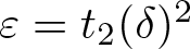 $\varepsilon=t_2(\delta)^2$ yields
 \begin{equation*}
\lim_{\delta\to \infty} h_{\varepsilon}(t_2(\delta))= \lim_{t_2\to 0}\frac{1-\frac{t_2(t_2+2t_2^2)}{(t_2+t_2^2)^2}\theta}{1+\frac{t_2(t_2+2t_2^2)}{(t_2+t_2^2)^2}\theta}=\lim_{t_2\to 0}\frac{1-\frac{(1+2t_2)}{(1+t_2)^2}\theta}{1+\frac{(1+2t_2)}{(1+t_2)^2}\theta}=\frac{1-\theta}{1+\theta}=\frac{1}{\lambda},
\end{equation*}
\begin{equation*}
\lim_{\delta\to \infty} h_{\varepsilon}(t_2(\delta))= \lim_{t_2\to 0}\frac{1-\frac{t_2(t_2+2t_2^2)}{(t_2+t_2^2)^2}\theta}{1+\frac{t_2(t_2+2t_2^2)}{(t_2+t_2^2)^2}\theta}=\lim_{t_2\to 0}\frac{1-\frac{(1+2t_2)}{(1+t_2)^2}\theta}{1+\frac{(1+2t_2)}{(1+t_2)^2}\theta}=\frac{1-\theta}{1+\theta}=\frac{1}{\lambda},
\end{equation*}which concludes the proof.
4.3. The sharpness of a weighted Hardy inequality
In this section, we present a sharpness result concerning a weighted Hardy inequality on 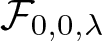 $\mathcal{F}_{0,0,\lambda}$. As a consequence, we also obtain theorem 1.1. Our result can be stated as follows.
Theorem 4.4. Let  $n\ge 3$,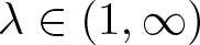 $\lambda\in (1,\infty)$, and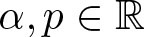 $\alpha,p\in \mathbb{R}$ such that $1 \lt p \lt n+\alpha$. For every $(\mathbb{R}^n,F_\varepsilon,\mathsf{m}_\varepsilon)\in \mathcal{F}_{0,0,\lambda}$ and $u\in C_0^\infty(\mathbb{R}^n)$ one has
 \begin{align}
\lambda^p\displaystyle\int_{\mathbb{R}^n} \rho^\alpha \cdot F_\varepsilon^*(Du)^p\,\mathrm{d} \mathsf{m}_\varepsilon\ge c_{n,p,\alpha}\int_{\mathbb{R}^n}\rho^\alpha\frac{u^p}{\rho_\varepsilon^p}\,\mathrm{d} \mathsf{m}_\varepsilon,\quad\text{where}\quad c_{n,p,\alpha}=\left(\frac{n+\alpha-p}{p}\right)^p.
\end{align}
\begin{align}
\lambda^p\displaystyle\int_{\mathbb{R}^n} \rho^\alpha \cdot F_\varepsilon^*(Du)^p\,\mathrm{d} \mathsf{m}_\varepsilon\ge c_{n,p,\alpha}\int_{\mathbb{R}^n}\rho^\alpha\frac{u^p}{\rho_\varepsilon^p}\,\mathrm{d} \mathsf{m}_\varepsilon,\quad\text{where}\quad c_{n,p,\alpha}=\left(\frac{n+\alpha-p}{p}\right)^p.
\end{align} Moreover,  $c_{n,p,\alpha}$ is sharp in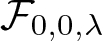 $\mathcal{F}_{0,0,\lambda}$, in the sense that it is the greatest constant with this property.
Proof. The proof of inequality (50) follows from theorem 3.3. To prove the sharpness, we use theorem 4.3. According to the relation (42), we obtain
 \begin{equation*}v(t)^p=\frac{1}{t^{n+\alpha-p}},\quad\forall t\in(0,\infty).\end{equation*}
For every δ > 1 define
 \begin{equation*}t_1(\delta)=\delta/2,\quad t_2(\delta)=\delta,\quad t_3(\delta)=\delta^2,\quad\mbox{and}\quad t_4(\delta)=2\delta^2.\end{equation*}
By simple computations, we obtain
 \begin{align*}
\frac{v(t_2)^p\cdot \mathcal{I}(w;t_1,t_2)}{(t_2-t_1)^p} & =\frac{2^{n+\alpha}-1}{(n+\alpha)2^{n+\alpha-p}}=\text{const}, \\
\frac{v(t_3)^p\cdot \mathcal{I}(w;t_3,t_4)}{(t_4-t_3)^p} & =\frac{2^{n+\alpha}-1}{n+\alpha}=\text{const}, \\
\mathcal{I}(wWv^p;t_2,t_3) & =c_{n,p,\alpha}\log(\delta)\to\infty,\quad\text{as } \delta\to\infty.
\end{align*}
\begin{align*}
\frac{v(t_2)^p\cdot \mathcal{I}(w;t_1,t_2)}{(t_2-t_1)^p} & =\frac{2^{n+\alpha}-1}{(n+\alpha)2^{n+\alpha-p}}=\text{const}, \\
\frac{v(t_3)^p\cdot \mathcal{I}(w;t_3,t_4)}{(t_4-t_3)^p} & =\frac{2^{n+\alpha}-1}{n+\alpha}=\text{const}, \\
\mathcal{I}(wWv^p;t_2,t_3) & =c_{n,p,\alpha}\log(\delta)\to\infty,\quad\text{as } \delta\to\infty.
\end{align*} It follows that 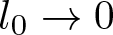 $l_0\to 0$ as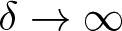 $\delta\to\infty$. Since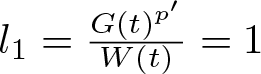 $l_1=\frac{G(t)^{p'}}{W(t)}=1$, for every t > 0, thus, theorem 4.3 yields the sharpness of the inequality (50).
We observe that choosing α = 0 and p = 2 in the above result yields theorem 1.1.
5. Sharp Hardy inequalities—strong negative curvature
In this section, we present our sharpness results concerning Hardy-type inequalities, assuming strong negative curvature. We proceed similarly to the previous case. In §5.1 we present a second construction of spaces (see theorem 5.1). In §5.2 we provide sufficient conditions for the sharpness of Hardy-type inequalities on them (see theorem 5.3). Finally, in §5.3 we present an application: In theorem 5.4 we prove a sharpness result concerning a McKean-type special gap estimate, which implies theorem 1.2.
5.1. Construction
Consider the triple 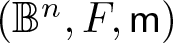 $(\mathbb{B}^n,F, \mathsf{m})$, where $\mathbb{B}^n$ denotes the Euclidean (open) unit ball, the function $F\colon \mathbb{B}^n\times \mathbb{R}^n\to [0,\infty)$ is defined by
 \begin{equation}
F(x,y)
=\frac{\sqrt{|y|^2-|x|^2|y|^2+\langle x,y\rangle^2}}{\kappa(1-\theta)(1-|x|^2)}-\frac{\theta\langle x,y\rangle}{\kappa(1-\theta) |x|(1-|x|^2)},
\end{equation}
\begin{equation}
F(x,y)
=\frac{\sqrt{|y|^2-|x|^2|y|^2+\langle x,y\rangle^2}}{\kappa(1-\theta)(1-|x|^2)}-\frac{\theta\langle x,y\rangle}{\kappa(1-\theta) |x|(1-|x|^2)},
\end{equation} for some 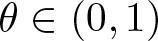 $\theta\in(0,1)$ and κ > 0; while $\mathsf{m}$ is a measure with density
 \begin{equation*}
\sigma= \exp(-(n-1)h \rho)\cdot \sigma_{F},
\end{equation*}
\begin{equation*}
\sigma= \exp(-(n-1)h \rho)\cdot \sigma_{F},
\end{equation*} for some 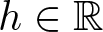 $h\in \mathbb{R}$. As before, ρ is the distance from the origin and σF is the density of the Busemann–Hausdorff measure induced by F. We observe that F is not a Finsler metric, since it is not continuous at the origin. However, for every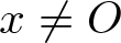 $x\ne O$, one has
 \begin{align*}
\mathbf{K}(x,x)=-\kappa^2,\quad \overline{\mathbf{S}}(x,x)=(n-1)h,\quad\mbox{and}\quad \mathbf{rev}(x,x)=\frac{1+\theta}{1-\theta}\stackrel{\textrm{def}}{=}\lambda=\lambda_F(\mathbb{B}^n).
\end{align*}
\begin{align*}
\mathbf{K}(x,x)=-\kappa^2,\quad \overline{\mathbf{S}}(x,x)=(n-1)h,\quad\mbox{and}\quad \mathbf{rev}(x,x)=\frac{1+\theta}{1-\theta}\stackrel{\textrm{def}}{=}\lambda=\lambda_F(\mathbb{B}^n).
\end{align*}The following result provides an approximation of the above structure by a family of Randers spaces.
Theorem 5.1. Let 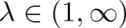 $\lambda\in(1,\infty)$,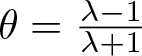 $\theta=\frac{\lambda-1}{\lambda+1}$, κ > 0 and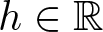 $h\in \mathbb{R}$. Construct the family $\mathcal{F}_{\kappa,h,\lambda}=\{(\mathbb{B}^n, F_\varepsilon,\mathsf{m}_\varepsilon)\}_{\varepsilon \gt 0}$ of FMMMs, where $F_\varepsilon\colon T\mathbb{B}^n\simeq\mathbb{B}^n\times\mathbb{R}^n\to [0,\infty)$ is defined by
 \begin{align*}
F_\varepsilon(x,y)& =\frac{\sqrt{|y|^2-|x|^2|y|^2+\langle x,y\rangle^2}}{k_{\varepsilon}(1-\theta)(1-|x|^2)}
-\frac{\theta \langle x,y\rangle}{k_{\varepsilon}(1-\theta) |x|(1-|x|^2)} \nonumber\\ & \quad \cdot \frac{\operatorname{arctanh}(|x|)\left(\operatorname{arctanh}(|x|)+2\varepsilon\right)}{\left(\operatorname{arctanh}(|x|)+\varepsilon\right)^2},
\end{align*}
\begin{align*}
F_\varepsilon(x,y)& =\frac{\sqrt{|y|^2-|x|^2|y|^2+\langle x,y\rangle^2}}{k_{\varepsilon}(1-\theta)(1-|x|^2)}
-\frac{\theta \langle x,y\rangle}{k_{\varepsilon}(1-\theta) |x|(1-|x|^2)} \nonumber\\ & \quad \cdot \frac{\operatorname{arctanh}(|x|)\left(\operatorname{arctanh}(|x|)+2\varepsilon\right)}{\left(\operatorname{arctanh}(|x|)+\varepsilon\right)^2},
\end{align*} kɛ is given by relation (54),  $\mathsf{m}_\varepsilon$ is a measure with density $\sigma_\varepsilon=\exp(-(n-1)h \rho_\varepsilon)\cdot \sigma_{F_\varepsilon}$, and $\sigma_{F_\varepsilon}$ denotes the density of the Busemann–Hausdorff measure induced by Fɛ. The following statements hold:
(i) For every ɛ > 0, the triple
$(\mathbb{B}^n, F_\varepsilon,\mathsf{m}_\varepsilon)$ is an FMMM. In addition, Fɛ is a projectively flat Randers metric, with reversibility
$\lambda_{F_\varepsilon}(\mathbb{B}^n)=\lambda$.(ii) For every
$x\in \mathbb{B}^n$ with
$x\ne 0$, one has
(52)\begin{align}
\mathbf{K}_\varepsilon(x,x)\to -\kappa^2,\quad \overline{\mathbf{S}}_\varepsilon(x,x)\to (n-1)h,\quad\mbox{and}\quad \mathbf{rev}_\varepsilon(x,x)\to\lambda,\quad\text{as}\quad \varepsilon\to 0.
\end{align}(iii) For every ɛ > 0 and
$x\in \mathbb{B}^n$, one has
(53)\begin{equation}
\mathbf{K}_\varepsilon(x,x)\le -\kappa^2,\quad
\overline{\mathbf{S}}_\varepsilon(x,x)\le (n-1)h,\quad\mbox{and}\quad
\mathbf{rev}_\varepsilon(x,x)\le\lambda.
\end{equation}
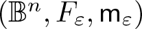

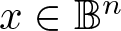


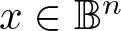

Proof. For simplicity of presentation, denote 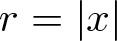 $r=|x|$, $\overline{r}=\operatorname{arctanh}(|x|)$, and $\vartheta_\varepsilon=k_\varepsilon(1-\theta)$. Using the standard notation of Randers metrics (see §2.3) one has
 \begin{equation*}
F_\varepsilon(x,y)=\sqrt{a_{ij}(x)y^iy^j}+b_i(x)y^i,
\end{equation*}
\begin{equation*}
F_\varepsilon(x,y)=\sqrt{a_{ij}(x)y^iy^j}+b_i(x)y^i,
\end{equation*}where
 \begin{equation*}
a_{ij}(x)=\frac{\delta_{ij}}{\vartheta_{\varepsilon}^2(1-r^2)}+\frac{x^ix^j}{\vartheta_{\varepsilon}^2(1-r^2)^2}
\quad\mbox{and}\quad
b_i(x)=-\frac{\theta \overline{r}(\overline{r}+2\varepsilon)x^i}{\vartheta_{\varepsilon} r(1-r^2)(\overline{r}+\varepsilon)^2}.
\end{equation*}
\begin{equation*}
a_{ij}(x)=\frac{\delta_{ij}}{\vartheta_{\varepsilon}^2(1-r^2)}+\frac{x^ix^j}{\vartheta_{\varepsilon}^2(1-r^2)^2}
\quad\mbox{and}\quad
b_i(x)=-\frac{\theta \overline{r}(\overline{r}+2\varepsilon)x^i}{\vartheta_{\varepsilon} r(1-r^2)(\overline{r}+\varepsilon)^2}.
\end{equation*} Let  $a^{ij}(x)=\{a_{ij}(x)\}^{-1}$, it follows that
 \begin{equation*}
\|b\|_a(x)=\sqrt{a^{ij}(x)b_i(x)b_j(x)}=\frac{\theta \overline{r}(\overline{r}+2\varepsilon)}{(\overline{r}+\varepsilon)^2} \lt \theta \lt 1.
\end{equation*}
\begin{equation*}
\|b\|_a(x)=\sqrt{a^{ij}(x)b_i(x)b_j(x)}=\frac{\theta \overline{r}(\overline{r}+2\varepsilon)}{(\overline{r}+\varepsilon)^2} \lt \theta \lt 1.
\end{equation*} Since Fɛ is also smooth, it is a Randers metric on  $\mathbb{R}^n$. According to remark 2.5, the metric Fɛ is projectively flat. Indeed, the Klein metric (obtained from Fɛ for θ = 0) is projectively flat, and
 \begin{equation*}
b_i\,\mathrm{d} x^i=D\beta(x),\quad\mbox{where}\quad
\beta(x)=-\frac{\theta}{\vartheta_{\varepsilon}}\left(\overline{r}+\frac{\varepsilon^2}{\overline{r}+\varepsilon}\right).
\end{equation*}
\begin{equation*}
b_i\,\mathrm{d} x^i=D\beta(x),\quad\mbox{where}\quad
\beta(x)=-\frac{\theta}{\vartheta_{\varepsilon}}\left(\overline{r}+\frac{\varepsilon^2}{\overline{r}+\varepsilon}\right).
\end{equation*} Let 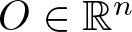 $O\in\mathbb{R}^n$ denote the origin, $\rho_\varepsilon(x)=d(O,x)$ and $\overleftarrow{\rho_\varepsilon} (x)=d(x,O)$. Then
 \begin{equation*}
\rho_\varepsilon(x)=\overline{r}\cdot \frac{\overline{r}(1-\theta)+ \varepsilon }{\vartheta_{\varepsilon}(\overline{r}+\varepsilon)}
\quad\mbox{and}\quad \overleftarrow{\rho_\varepsilon} (x) =\overline{r}\cdot \frac{\overline{r}(1+\theta)+ \varepsilon }{\vartheta_{\varepsilon}(\overline{r}+\varepsilon)}.
\end{equation*}
\begin{equation*}
\rho_\varepsilon(x)=\overline{r}\cdot \frac{\overline{r}(1-\theta)+ \varepsilon }{\vartheta_{\varepsilon}(\overline{r}+\varepsilon)}
\quad\mbox{and}\quad \overleftarrow{\rho_\varepsilon} (x) =\overline{r}\cdot \frac{\overline{r}(1+\theta)+ \varepsilon }{\vartheta_{\varepsilon}(\overline{r}+\varepsilon)}.
\end{equation*}In addition, one has
 \begin{equation*}
D\rho_\varepsilon(x)=\left(\frac{(\overline{r}+\varepsilon)^2-\overline{r}(\overline{r}+2\varepsilon)\theta}{\vartheta_{\varepsilon}r(1-r^2)(\overline{r}+\varepsilon )^2}\right)\cdot x
\quad\mbox{and}\quad
\nabla\rho_\varepsilon(x)=\frac{\vartheta_{\varepsilon}(1-r^2)(\overline{r}+\varepsilon)^2}{r((\overline{r}+\varepsilon)^2-\overline{r}(\overline{r}+2\varepsilon)\theta)}\cdot x.
\end{equation*}
\begin{equation*}
D\rho_\varepsilon(x)=\left(\frac{(\overline{r}+\varepsilon)^2-\overline{r}(\overline{r}+2\varepsilon)\theta}{\vartheta_{\varepsilon}r(1-r^2)(\overline{r}+\varepsilon )^2}\right)\cdot x
\quad\mbox{and}\quad
\nabla\rho_\varepsilon(x)=\frac{\vartheta_{\varepsilon}(1-r^2)(\overline{r}+\varepsilon)^2}{r((\overline{r}+\varepsilon)^2-\overline{r}(\overline{r}+2\varepsilon)\theta)}\cdot x.
\end{equation*}According to relation (23), the density of the Busemann–Hausdorff measure induced by Fɛ is
 \begin{equation*}
\sigma_{F_\varepsilon}=
\frac{1}{\vartheta_{\varepsilon}^n}\cdot\left(\frac{1}{1-r^2}\right)^\frac{n+1}{2}\cdot\left(1-\frac{\overline{r}^2 (\overline{r}+2 \varepsilon)^2\theta^2}{(\overline{r}+\varepsilon)^4}\right)^\frac{n+1}{2}
\stackrel{\textrm{def}}{=} \frac{1}{\vartheta_{\varepsilon}^n}\cdot
\left(\frac{1}{1-\overline{r}^2}\right)^\frac{n+1}{2}
\cdot f_\varepsilon^\frac{n+1}{2}.
\end{equation*}
\begin{equation*}
\sigma_{F_\varepsilon}=
\frac{1}{\vartheta_{\varepsilon}^n}\cdot\left(\frac{1}{1-r^2}\right)^\frac{n+1}{2}\cdot\left(1-\frac{\overline{r}^2 (\overline{r}+2 \varepsilon)^2\theta^2}{(\overline{r}+\varepsilon)^4}\right)^\frac{n+1}{2}
\stackrel{\textrm{def}}{=} \frac{1}{\vartheta_{\varepsilon}^n}\cdot
\left(\frac{1}{1-\overline{r}^2}\right)^\frac{n+1}{2}
\cdot f_\varepsilon^\frac{n+1}{2}.
\end{equation*} Observe that  $1-\theta^2\le f_\varepsilon\le 1$. The density of $\mathsf{m}_\varepsilon$ is
 \begin{equation*}
\sigma_\varepsilon= \exp\left(-(n-1)h\rho_\varepsilon\right)\cdot \frac{1}{\vartheta_{\varepsilon}^n}\left(\frac{1}{1-\overline{r}^2}\right)^\frac{n+1}{2}f_\varepsilon^\frac{n+1}{2}.
\end{equation*}
\begin{equation*}
\sigma_\varepsilon= \exp\left(-(n-1)h\rho_\varepsilon\right)\cdot \frac{1}{\vartheta_{\varepsilon}^n}\left(\frac{1}{1-\overline{r}^2}\right)^\frac{n+1}{2}f_\varepsilon^\frac{n+1}{2}.
\end{equation*} In the sequel, we compute the flag curvature, the reduced S-curvature, and the reversibility of 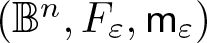 $(\mathbb{B}^n,F_\varepsilon,\mathsf{m}_\varepsilon)$ along the geodesics starting from O. Recall that $\vartheta_\varepsilon=k_\varepsilon(1-\theta)$. Concerning the flag curvature, we obtain
 \begin{align*}
\mathbf{K}_{\rho_\varepsilon}(\overline{r})\stackrel{\textrm{def}}{=}\mathbf{K}_\varepsilon(x,x)=
-\frac{k_{\varepsilon}^2(1-\theta)^2(\overline{r}+\varepsilon )^4
\left(e_0-e_1\theta +e_2\theta^2
\right)}{\left((\overline{r}+\varepsilon )^2-\overline{r} (\overline{r}+2 \varepsilon )\theta \right)^4},
\end{align*}
\begin{align*}
\mathbf{K}_{\rho_\varepsilon}(\overline{r})\stackrel{\textrm{def}}{=}\mathbf{K}_\varepsilon(x,x)=
-\frac{k_{\varepsilon}^2(1-\theta)^2(\overline{r}+\varepsilon )^4
\left(e_0-e_1\theta +e_2\theta^2
\right)}{\left((\overline{r}+\varepsilon )^2-\overline{r} (\overline{r}+2 \varepsilon )\theta \right)^4},
\end{align*} where  $e_0=(\overline{r}+\varepsilon)^4$, $e_1=2\overline{r}^4+8\overline{r}^3\varepsilon+(10\overline{r}^2-3)\varepsilon^2+4\overline{r}\varepsilon^3$, and $e_2=\overline{r}^4+4\overline{r}^3\varepsilon+(4\overline{r}^2-3)\varepsilon^2$.
Our goal is to choose kɛ such that relations (52) and (53) hold. For every ɛ > 0, one has
 \begin{align*}
&\lim_{\overline{r}\to\infty} \mathbf{K}_{\rho_\varepsilon}(\overline{r}) =-k_{\varepsilon}^2,\quad\text{and}\quad
\lim_{\overline{r}\to0} \mathbf{K}_{\rho_\varepsilon}(\overline{r}) =-k_{\varepsilon}^2\cdot K_{\varepsilon,0},\nonumber\\ & \quad \text{where}\quad K_{\varepsilon,0}=(1-\theta)^2\left(1+\frac{3\theta(1-\theta)}{\varepsilon^2}\right).
\end{align*}
\begin{align*}
&\lim_{\overline{r}\to\infty} \mathbf{K}_{\rho_\varepsilon}(\overline{r}) =-k_{\varepsilon}^2,\quad\text{and}\quad
\lim_{\overline{r}\to0} \mathbf{K}_{\rho_\varepsilon}(\overline{r}) =-k_{\varepsilon}^2\cdot K_{\varepsilon,0},\nonumber\\ & \quad \text{where}\quad K_{\varepsilon,0}=(1-\theta)^2\left(1+\frac{3\theta(1-\theta)}{\varepsilon^2}\right).
\end{align*} By a simple derivative test, we obtain that if 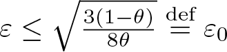 $\varepsilon\le \sqrt{\frac{3(1-\theta)}{8\theta}}\stackrel{\textrm{def}}{=} \varepsilon_0$, then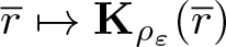 $\overline{r}\mapsto\mathbf{K}_{\rho_\varepsilon}(\overline{r})$ admits a unique maximum on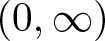 $(0,\infty)$, which is given by
 \begin{align*}
& -k_{\varepsilon}^2\cdot K_{\varepsilon}, \quad\text{where}\quad K_{\varepsilon}\nonumber\\ & \quad =\frac{6(1-\theta)^2\left((1-\theta ) \left(3 (1-\theta )-2 \varepsilon ^2 \theta \right)+\sqrt{3 (1-\theta)^3 \left(3(1-\theta)-8 \varepsilon ^2 \theta \right)}\right)^3}{\left(3 (1-\theta )^2+\sqrt{3 (1-\theta)^3 \left(3(1-\theta)-8 \varepsilon ^2 \theta \right)}\right)^4}\le 1.
\end{align*}
\begin{align*}
& -k_{\varepsilon}^2\cdot K_{\varepsilon}, \quad\text{where}\quad K_{\varepsilon}\nonumber\\ & \quad =\frac{6(1-\theta)^2\left((1-\theta ) \left(3 (1-\theta )-2 \varepsilon ^2 \theta \right)+\sqrt{3 (1-\theta)^3 \left(3(1-\theta)-8 \varepsilon ^2 \theta \right)}\right)^3}{\left(3 (1-\theta )^2+\sqrt{3 (1-\theta)^3 \left(3(1-\theta)-8 \varepsilon ^2 \theta \right)}\right)^4}\le 1.
\end{align*} For simplicity define 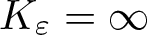 $K_{\varepsilon}=\infty$, when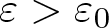 $\varepsilon \gt \varepsilon_0$. To ensure $\mathbf{K}_{\rho_\varepsilon}(\overline{r})\le-\kappa^2$, $\forall \varepsilon \gt 0,\overline{r}\ge 0$, choose
 \begin{equation}
k_{\varepsilon}=\max\left\{\kappa,\frac{\kappa}{\sqrt{K_{\varepsilon,0}}},\frac{\kappa}{\sqrt{K_{\varepsilon}}}\right\}.
\end{equation}
\begin{equation}
k_{\varepsilon}=\max\left\{\kappa,\frac{\kappa}{\sqrt{K_{\varepsilon,0}}},\frac{\kappa}{\sqrt{K_{\varepsilon}}}\right\}.
\end{equation} If ɛ → 0, then 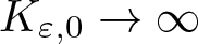 $K_{\varepsilon,0}\to\infty$,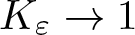 $K_\varepsilon\to1$, and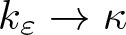 $k_{\varepsilon}\to\kappa$. Thus, for every $\overline{r} \gt 0$ we obtain $\mathbf{K}_{\rho_\varepsilon}(\overline{r})\to-\kappa^2$ as ɛ → 0.
The reduced S-curvature along ρɛ can be computed as
 \begin{align*}
\overline{\mathbf{S}}_{\rho_\varepsilon}(\overline{r})\stackrel{\textrm{def}}{=}\overline{\mathbf{S}}(x,x)
& = (n-1)h-\frac{\vartheta_{\varepsilon}(n+1)(\overline{r}+\varepsilon)\theta \varepsilon^2}{(\overline{r}+\varepsilon)^4-\overline{r}^2(\overline{r}+2\varepsilon)^2\theta^2}\le (n-1)h.
\end{align*}
\begin{align*}
\overline{\mathbf{S}}_{\rho_\varepsilon}(\overline{r})\stackrel{\textrm{def}}{=}\overline{\mathbf{S}}(x,x)
& = (n-1)h-\frac{\vartheta_{\varepsilon}(n+1)(\overline{r}+\varepsilon)\theta \varepsilon^2}{(\overline{r}+\varepsilon)^4-\overline{r}^2(\overline{r}+2\varepsilon)^2\theta^2}\le (n-1)h.
\end{align*} We easily obtain that if  $\overline{r} \gt 0$, then $\overline{\mathbf{S}}_{\rho_\varepsilon}(\overline{r})\to (n-1)h$ as ɛ → 0. If $\overline{r}=0$, then $\overline{\mathbf{S}}_{\rho_\varepsilon}(\overline{r})\to -\infty$ as ɛ → 0. In addition, for every fixed ɛ > 0 one has $\overline{\mathbf{S}}_{\rho_\varepsilon}(\overline{r})\to (n-1)h$ as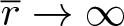 $\overline{r}\to \infty$.
Finally, for the reversibility we obtain
 \begin{equation*}
\mathbf{rev}_{\rho_\varepsilon}(\overline{r})\stackrel{\textrm{def}}{=}\mathbf{rev}(x,x)=\frac{1+\frac{\overline{r}(\overline{r}+2\varepsilon)\theta}{(\overline{r}+\varepsilon)^2}}{1-\frac{\overline{r}(\overline{r}+2\varepsilon)\theta}{(\overline{r}+\varepsilon)^2}}\le \frac{1+\theta}{1-\theta}=\lambda.
\end{equation*}
\begin{equation*}
\mathbf{rev}_{\rho_\varepsilon}(\overline{r})\stackrel{\textrm{def}}{=}\mathbf{rev}(x,x)=\frac{1+\frac{\overline{r}(\overline{r}+2\varepsilon)\theta}{(\overline{r}+\varepsilon)^2}}{1-\frac{\overline{r}(\overline{r}+2\varepsilon)\theta}{(\overline{r}+\varepsilon)^2}}\le \frac{1+\theta}{1-\theta}=\lambda.
\end{equation*} It follows that, if  $\overline{r} \gt 0$, then $\mathbf{rev}_{\rho_\varepsilon}(\overline{r})\to\lambda$ as ɛ → 0, and for every fixed ɛ > 0 one has $\mathbf{rev}_{\rho_\varepsilon}(\overline{r})\to \lambda$ as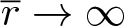 $\overline{r}\to \infty$, and $\mathbf{rev}_{\rho_\varepsilon}(\overline{r})\to 1$ as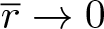 $\overline{r}\to 0$. The latter limit ensures the continuity of Fɛ at the origin. In addition, $\lambda_{F_\varepsilon}(\mathbb{B}^n)=\lambda$, for every ɛ > 0. Indeed, for every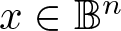 $x\in \mathbb{B}^n$, and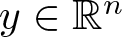 $y\in \mathbb{R}^n$ one has
 \begin{equation*}\mathbf{rev}_\varepsilon(x,y)=\frac{F_\varepsilon(x,-y)}{F_\varepsilon(x,y)}\le \frac{F_\varepsilon(x,-x)}{F_\varepsilon(x,x)}=\mathbf{rev}_\varepsilon(x,x)\le \lambda,\quad \text{if }x\ne O, \quad\text{and}\quad \mathbf{rev}_\varepsilon(O,y)=1,\end{equation*}
which concludes the proof.
We make the following observations.
(a) Although there exist various formal similarities between theorems 4.1 and 5.1, we highlight a main difference, which is the monotonicity of
${r}\mapsto \mathbf{K}_{\rho_\varepsilon}({r})$. In case of non-positive curvature this function is increasing, hence its limit as
${r}\to\infty$ is its upper bound. In case of strong negative curvature, for sufficiently small ɛ, it increases to a global maximum
$-k^2_{\varepsilon,\vartheta}\cdot K_\varepsilon$ then decreases (in the proof, that maximum was adjusted to ensure the required upper bound).It is an interesting question, if there exists a perturbation of the metric (51) (or some other construction), in which
$\mathbf{K}\le-\kappa^2$ along
$\nabla\rho_\varepsilon$ with a strictly increasing flag curvature along
$\nabla\rho_\varepsilon$, or if this phenomenon is directly implied by the constraints on the geometry. We note that on each alternative prototypes of families of spaces that were examined during the research, the same phenomena occurred.(b) As we anticipated in remark 4.2(b), the construction of the measure
$\mathsf{m}_\varepsilon$ allows for non-zero upper bound of the reduced S-curvature, which is particularly important for our applications.(c) Since
$K_{\varepsilon,0}\to\infty$ as ɛ → 0, there exists
$\varepsilon_1\in(0,\varepsilon_0)$ such that
$k_\varepsilon=\frac{\kappa}{\sqrt{K_\varepsilon}}$, for every
$\varepsilon\in(0,\varepsilon_1)$. Moreover, since
$k_\varepsilon\to\kappa$ from above, there exist
$\overline \varepsilon\in (0,\varepsilon_1)$ and
$\overline \kappa \gt \kappa$, such that
(55)\begin{equation}
\kappa \le k_{\varepsilon}\le \overline \kappa,\quad\forall \varepsilon\in(0,\overline\varepsilon).
\end{equation}(d) Similarly to remark 4.2(d), we have
$\max\{F^{*}_\varepsilon(\pm D\rho_\varepsilon)\}=F^{*}_\varepsilon(D\rho_\varepsilon)=1$, since
(56)\begin{equation}
F^*_\varepsilon(-D\rho_\varepsilon)=\frac{1-\frac{\overline{r}(\overline{r}+2\varepsilon)}{(\overline{r}+\varepsilon)^2}\theta}{1+\frac{\overline{r}(\overline{r}+2\varepsilon)}{(\overline{r}+\varepsilon)^2}\theta}\stackrel{\textrm{def}}{=} h_\varepsilon(\overline{r}),\quad\mbox{where}\quad \frac{1-\theta}{1+\theta}\le h_\varepsilon(\overline{r})\le1.
\end{equation}
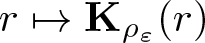

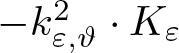
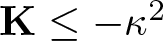


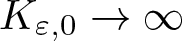
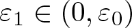
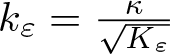
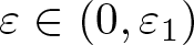
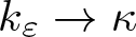
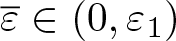
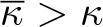



5.2. Sufficient conditions for sharpness
In this section, we present sufficient conditions for the sharpness of Hardy inequalities on the spaces of 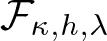 $\mathcal{F}_{\kappa,h,\lambda}$, introduced in theorem 5.1.
Let  $(\mathbb{B}^n,F_\varepsilon,\mathsf{m}_\varepsilon)\subset \mathcal{F}_{\kappa,h,\lambda}$ for some ɛ > 0,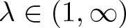 $\lambda\in(1,\infty)$, κ > 0 and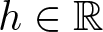 $h\in \mathbb{R}$. Then for every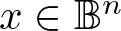 $x\in \mathbb{B}^n$, one has
 \begin{equation*}
\mathbf{K}_{\varepsilon}(x,x)\le-\kappa^2,\quad \overline{\mathbf{S}}_{\varepsilon}(x,x)\le (n-1)h,\quad\text{and}\quad \mathbf{rev}_{\varepsilon}(x,x)\le \lambda=\lambda_{F_\varepsilon}(\mathbb{B}^n).
\end{equation*}
\begin{equation*}
\mathbf{K}_{\varepsilon}(x,x)\le-\kappa^2,\quad \overline{\mathbf{S}}_{\varepsilon}(x,x)\le (n-1)h,\quad\text{and}\quad \mathbf{rev}_{\varepsilon}(x,x)\le \lambda=\lambda_{F_\varepsilon}(\mathbb{B}^n).
\end{equation*}Denote by ρɛ the distance from the origin. By the Laplace comparison theorem (see theorem 2.2) one has
 \begin{equation*}
\Delta_{F_\varepsilon} (\rho_\varepsilon)\ge (n-1)\kappa\coth(\kappa\rho_\varepsilon)-(n-1)h\stackrel{\textrm{def}}{=} L^{\kappa,h}(\rho_\varepsilon).
\end{equation*}
\begin{equation*}
\Delta_{F_\varepsilon} (\rho_\varepsilon)\ge (n-1)\kappa\coth(\kappa\rho_\varepsilon)-(n-1)h\stackrel{\textrm{def}}{=} L^{\kappa,h}(\rho_\varepsilon).
\end{equation*} Let  $R\in(0,+\infty]$, $L(t)\le L^{\kappa,h}(t)$ for every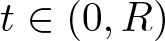 $t\in(0,R)$, and define
 \begin{equation*}
\Omega_\varepsilon=\{x\in \mathbb{B}^n\mid \rho_\varepsilon(x) \lt R\}.
\end{equation*}
\begin{equation*}
\Omega_\varepsilon=\{x\in \mathbb{B}^n\mid \rho_\varepsilon(x) \lt R\}.
\end{equation*} Suppose that (L, W) is a 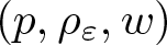 $(p,\rho_\varepsilon,w)$-Riccati pair in $(0,R)$, that is $W\colon(0,R)\to (0,\infty)$ is continuous, $w\colon(0,R)\to (0,\infty)$ is of class C 1, and there exists $G\colon(0,R)\to(0,\infty)$ of class C 1 such that
 \begin{equation}
(G(t)w(t))'+G(t)w(t)L(t)-(p-1)G(t)^{p'}w(t)\geq W(t)w(t), \quad\forall t\in (0,R).
\end{equation}
\begin{equation}
(G(t)w(t))'+G(t)w(t)L(t)-(p-1)G(t)^{p'}w(t)\geq W(t)w(t), \quad\forall t\in (0,R).
\end{equation} By theorem 3.1, for every  $u\in C_0^\infty(\Omega_\varepsilon)$ one has
 \begin{align}
\lambda^p\int_{\Omega_\varepsilon} w(\rho_\varepsilon) F^*_\varepsilon(Du)^p\,\mathrm{d} \mathsf{m}_\varepsilon
& \ge\int_{\Omega_\varepsilon} w(\rho_\varepsilon) W(\rho_\varepsilon) |u|^p\,\mathrm{d} \mathsf{m}_\varepsilon.
\end{align}
\begin{align}
\lambda^p\int_{\Omega_\varepsilon} w(\rho_\varepsilon) F^*_\varepsilon(Du)^p\,\mathrm{d} \mathsf{m}_\varepsilon
& \ge\int_{\Omega_\varepsilon} w(\rho_\varepsilon) W(\rho_\varepsilon) |u|^p\,\mathrm{d} \mathsf{m}_\varepsilon.
\end{align} Suppose that G > 0 satisfies the Riccati ODI (57) with equality, and define  $v\colon (0,R)\to\mathbb{R}$ by
 \begin{equation}
-(\log v(t))'=-\frac{v'(t)}{v(t)}=G(t)^\frac{1}{p-1}.
\end{equation}
\begin{equation}
-(\log v(t))'=-\frac{v'(t)}{v(t)}=G(t)^\frac{1}{p-1}.
\end{equation}Since G is smooth and positive, v is smooth, positive, and decreasing. Introduce the notation
 \begin{equation}
\mathcal{I}^{k,h}(f;a,b)=\int_a^b f(t)\sinh(k t)^{n-1}e^{-(n-1)h t}\,\mathrm{d} t,
\end{equation}
\begin{equation}
\mathcal{I}^{k,h}(f;a,b)=\int_a^b f(t)\sinh(k t)^{n-1}e^{-(n-1)h t}\,\mathrm{d} t,
\end{equation} where 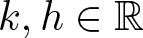 $k,h\in \mathbb{R}$ and $f\colon[a,b]\to\mathbb{R}$ is a continuous function, with $0 \lt a \lt b \lt R$. We have the following result.
Theorem 5.3. Fix 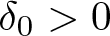 $\delta_0 \gt 0$ and let $t_1=t_1(\delta),t_2=t_2(\delta),t_3=t_3(\delta),t_4=t_4(\delta)$ be continuous functions admitting a (possibly infinite) limit at infinity, such that for every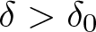 $\delta \gt \delta_0$ one has $0 \lt t_1 \lt t_2 \lt t_3 \lt t_4 \lt R$. Let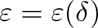 $\varepsilon=\varepsilon(\delta)$ such that ɛ → 0, as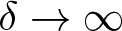 $\delta\to\infty$, and suppose that the following limits hold true:
 \begin{align*}
\lim_{\delta\to\infty} l_0^{k_\varepsilon,h}(\delta) & =0,\quad\mbox{where}\quad l_0^{k_\varepsilon,h}(\delta)\stackrel{\textrm{def}}{=} \frac{v(t_2)^p\cdot \mathcal{I}^{k_\varepsilon,h}(w;t_1,t_2)}{(t_2-t_1)^p\cdot \mathcal{I}^{k_\varepsilon,h}(wW v^p;t_2,t_3)}\nonumber\\ & \quad +\frac{v(t_3)^p\cdot \mathcal{I}^{k_\varepsilon,h}(w;t_3,t_4)}{(t_4-t_3)^p\cdot \mathcal{I}^{k_\varepsilon,h}(wW v^p;t_2,t_3)}, \\
\lim_{\delta\to\infty} l_1^{k_\varepsilon,h}(\delta) & =1,\quad\mbox{where}\quad l_1^{k_\varepsilon,h}(\delta)\stackrel{\textrm{def}}{=}\max_{t\in [t_2,t_3]} \frac{G(t)^{p'}}{W (t)},\\
\lim_{\delta\to\infty}l_2^{k_\varepsilon,h}(\delta) &=\frac{1}{\lambda}\quad\text{where}\quad l_2^{k_\varepsilon,h}(\delta)\stackrel{\textrm{def}}{=} h_\varepsilon((1-\theta)\kappa t_2),\quad\textrm{(see relation~{eq:k:he})}.
\end{align*}
\begin{align*}
\lim_{\delta\to\infty} l_0^{k_\varepsilon,h}(\delta) & =0,\quad\mbox{where}\quad l_0^{k_\varepsilon,h}(\delta)\stackrel{\textrm{def}}{=} \frac{v(t_2)^p\cdot \mathcal{I}^{k_\varepsilon,h}(w;t_1,t_2)}{(t_2-t_1)^p\cdot \mathcal{I}^{k_\varepsilon,h}(wW v^p;t_2,t_3)}\nonumber\\ & \quad +\frac{v(t_3)^p\cdot \mathcal{I}^{k_\varepsilon,h}(w;t_3,t_4)}{(t_4-t_3)^p\cdot \mathcal{I}^{k_\varepsilon,h}(wW v^p;t_2,t_3)}, \\
\lim_{\delta\to\infty} l_1^{k_\varepsilon,h}(\delta) & =1,\quad\mbox{where}\quad l_1^{k_\varepsilon,h}(\delta)\stackrel{\textrm{def}}{=}\max_{t\in [t_2,t_3]} \frac{G(t)^{p'}}{W (t)},\\
\lim_{\delta\to\infty}l_2^{k_\varepsilon,h}(\delta) &=\frac{1}{\lambda}\quad\text{where}\quad l_2^{k_\varepsilon,h}(\delta)\stackrel{\textrm{def}}{=} h_\varepsilon((1-\theta)\kappa t_2),\quad\textrm{(see relation~{eq:k:he})}.
\end{align*} Then inequality (58) is sharp on 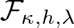 $\mathcal{F}_{\kappa,h,\lambda}$ in the sense that it no longer holds on each FMMM of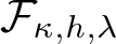 $\mathcal{F}_{\kappa,h,\lambda}$ if we multiply its right-hand side by a constant c > 1.
Proof. Let ɛ > 0 and  $T=(t_1,t_2,t_3,t_4)$. As before, define the limit function $u^\star_\varepsilon \colon \Omega\to (0,\infty)$ of (58) and its truncation $u^\star_{\varepsilon,T}$ by
 \begin{equation*}u^\star_\varepsilon(x)=v(\rho_\varepsilon(x)),\quad\mbox{and}\quad u^\star_{\varepsilon,T}(x)=v_{\varepsilon,T}(\rho_\varepsilon(x)),\end{equation*}
where
 \begin{equation}
v_{\varepsilon,T}(t)=\begin{cases}
0, & \mbox{if }0 \lt t\le t_1, \\
v(t_2)\frac{t-t_1}{t_2-t_1}, & \mbox{if }t_1\le t\le t_2, \\
v(t), & \mbox{if }t_2\le t\le t_3, \\
v(t_3)\frac{t_4-t}{t_4-t_3}, & \mbox{if }t_3\le t\le t_4, \\
0, & \mbox{if }t_4\le t \lt R,
\end{cases}\quad\mbox{and}\quad v_{\varepsilon,T}'(t)=\begin{cases}
0, & \mbox{if }0 \lt t \lt t_1, \\
\frac{v(t_2)}{t_2-t_1}, & \mbox{if }t_1 \lt t \lt t_2, \\
v'(t), & \mbox{if }t_2 \lt t \lt t_3, \\
-\frac{v(t_3)}{t_4-t_3}, & \mbox{if }t_3 \lt t \lt t_4, \\
0, & \mbox{if }t_4 \lt t \lt R.
\end{cases}
\end{equation}
\begin{equation}
v_{\varepsilon,T}(t)=\begin{cases}
0, & \mbox{if }0 \lt t\le t_1, \\
v(t_2)\frac{t-t_1}{t_2-t_1}, & \mbox{if }t_1\le t\le t_2, \\
v(t), & \mbox{if }t_2\le t\le t_3, \\
v(t_3)\frac{t_4-t}{t_4-t_3}, & \mbox{if }t_3\le t\le t_4, \\
0, & \mbox{if }t_4\le t \lt R,
\end{cases}\quad\mbox{and}\quad v_{\varepsilon,T}'(t)=\begin{cases}
0, & \mbox{if }0 \lt t \lt t_1, \\
\frac{v(t_2)}{t_2-t_1}, & \mbox{if }t_1 \lt t \lt t_2, \\
v'(t), & \mbox{if }t_2 \lt t \lt t_3, \\
-\frac{v(t_3)}{t_4-t_3}, & \mbox{if }t_3 \lt t \lt t_4, \\
0, & \mbox{if }t_4 \lt t \lt R.
\end{cases}
\end{equation}Proceeding similarly to the proof of theorem 4.3, we reduce the following integrals to one dimension:
 \begin{equation*}
I\stackrel{\textrm{def}}{=} \frac{1}{n\omega}\int_{\Omega_\varepsilon} w(\rho_\varepsilon) F^*_\varepsilon(Du^\star_{\varepsilon,T})^p\,\mathrm{d} \mathsf{m}_\varepsilon\quad\mbox{and}\quad
J\stackrel{\textrm{def}}{=}\frac{1}{n\omega}\int_{\Omega_\varepsilon} w(\rho_\varepsilon) W(\rho_\varepsilon) (u_{\varepsilon,T}^\star)^p\,\mathrm{d} \mathsf{m}_\varepsilon.
\end{equation*}
\begin{equation*}
I\stackrel{\textrm{def}}{=} \frac{1}{n\omega}\int_{\Omega_\varepsilon} w(\rho_\varepsilon) F^*_\varepsilon(Du^\star_{\varepsilon,T})^p\,\mathrm{d} \mathsf{m}_\varepsilon\quad\mbox{and}\quad
J\stackrel{\textrm{def}}{=}\frac{1}{n\omega}\int_{\Omega_\varepsilon} w(\rho_\varepsilon) W(\rho_\varepsilon) (u_{\varepsilon,T}^\star)^p\,\mathrm{d} \mathsf{m}_\varepsilon.
\end{equation*} For simplicity, denote 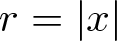 $r=|x|$, $\overline{r}=\operatorname{arctanh}(r)$, and $\vartheta_{\varepsilon}=k_\varepsilon(1-\theta)$. Introduce the following notations:
 \begin{align*}
t\stackrel{\textrm{def}}{=}\rho_\varepsilon(x)=\overline{r}\cdot \frac{\overline{r}(1-\theta)+ \varepsilon }{\vartheta_{\varepsilon}(\overline{r}+\varepsilon)}
\quad\text{and}\quad e(t)\stackrel{\textrm{def}}{=} \exp(-(n-1)ht).
\end{align*}
\begin{align*}
t\stackrel{\textrm{def}}{=}\rho_\varepsilon(x)=\overline{r}\cdot \frac{\overline{r}(1-\theta)+ \varepsilon }{\vartheta_{\varepsilon}(\overline{r}+\varepsilon)}
\quad\text{and}\quad e(t)\stackrel{\textrm{def}}{=} \exp(-(n-1)ht).
\end{align*}By a simple computation, we obtain that
 \begin{align*}
r & =\tanh \varphi_\varepsilon(t), & \text{where}\quad \varphi_\varepsilon(t) & =\frac{t\vartheta_\varepsilon -\varepsilon+\sqrt{(t\vartheta_\varepsilon -\varepsilon)^2+4t\vartheta_\varepsilon\varepsilon(1-\theta)}}{2(1-\theta)}, \\
\,\mathrm{d} r & =\frac{1}{(\cosh\varphi_\varepsilon(t))^2}\varphi_\varepsilon'(t)\,\mathrm{d} t, & \text{where}\quad \varphi_\varepsilon'(t) & =\frac{k}{2}\left(1+\frac{t\vartheta_\varepsilon-\varepsilon+2\varepsilon(1-\theta)}{\sqrt{(t\vartheta_\varepsilon -\varepsilon)^2+4t\vartheta_\varepsilon\varepsilon(1-\theta)}}\right) , \\
\sigma_\varepsilon & = e(t)\cdot \frac{1}{\vartheta_\varepsilon^n} (\cosh\varphi_\varepsilon(t))^{n+1} (f_\varepsilon(t))^\frac{n+1}{2}, &
\text{where}\quad f_\varepsilon(t) & =1-\frac{\varphi_\varepsilon^2(t) (\varphi_\varepsilon(t)+2 \varepsilon)^2\theta^2}{(\varphi_\varepsilon(t)+\varepsilon)^4}.
\end{align*}
\begin{align*}
r & =\tanh \varphi_\varepsilon(t), & \text{where}\quad \varphi_\varepsilon(t) & =\frac{t\vartheta_\varepsilon -\varepsilon+\sqrt{(t\vartheta_\varepsilon -\varepsilon)^2+4t\vartheta_\varepsilon\varepsilon(1-\theta)}}{2(1-\theta)}, \\
\,\mathrm{d} r & =\frac{1}{(\cosh\varphi_\varepsilon(t))^2}\varphi_\varepsilon'(t)\,\mathrm{d} t, & \text{where}\quad \varphi_\varepsilon'(t) & =\frac{k}{2}\left(1+\frac{t\vartheta_\varepsilon-\varepsilon+2\varepsilon(1-\theta)}{\sqrt{(t\vartheta_\varepsilon -\varepsilon)^2+4t\vartheta_\varepsilon\varepsilon(1-\theta)}}\right) , \\
\sigma_\varepsilon & = e(t)\cdot \frac{1}{\vartheta_\varepsilon^n} (\cosh\varphi_\varepsilon(t))^{n+1} (f_\varepsilon(t))^\frac{n+1}{2}, &
\text{where}\quad f_\varepsilon(t) & =1-\frac{\varphi_\varepsilon^2(t) (\varphi_\varepsilon(t)+2 \varepsilon)^2\theta^2}{(\varphi_\varepsilon(t)+\varepsilon)^4}.
\end{align*}It follows that
 \begin{align}
\sigma_\varepsilon r^{n-1}\,\mathrm{d} r
& =
e(t)\cdot\varphi'_\varepsilon(t)
\frac{1}{\vartheta_\varepsilon^n}(f_\varepsilon(t))^\frac{n+1}{2}
(\sinh \varphi_\varepsilon(t))^{n-1}\,\mathrm{d} t
\stackrel{\textrm{def}}{=} e(t)\cdot\psi_\varepsilon(t)\,\mathrm{d} t.
\end{align}
\begin{align}
\sigma_\varepsilon r^{n-1}\,\mathrm{d} r
& =
e(t)\cdot\varphi'_\varepsilon(t)
\frac{1}{\vartheta_\varepsilon^n}(f_\varepsilon(t))^\frac{n+1}{2}
(\sinh \varphi_\varepsilon(t))^{n-1}\,\mathrm{d} t
\stackrel{\textrm{def}}{=} e(t)\cdot\psi_\varepsilon(t)\,\mathrm{d} t.
\end{align} In the sequel, we provide suitable bounds for  $\psi_\varepsilon(t)$. First, we observe that
 \begin{equation*}
(1-\theta)k_\varepsilon t \le \varphi_\varepsilon(t)\le k_\varepsilon t,\quad
(1-\theta)k_\varepsilon \le \varphi_\varepsilon'(t)\le k_\varepsilon,\quad\mbox{and}\quad
1-\theta^2 \le f_\varepsilon(t)\le 1,\quad \forall t\ge 0.
\end{equation*}
\begin{equation*}
(1-\theta)k_\varepsilon t \le \varphi_\varepsilon(t)\le k_\varepsilon t,\quad
(1-\theta)k_\varepsilon \le \varphi_\varepsilon'(t)\le k_\varepsilon,\quad\mbox{and}\quad
1-\theta^2 \le f_\varepsilon(t)\le 1,\quad \forall t\ge 0.
\end{equation*} Next, we show that there exists  $\widetilde{\varepsilon} \gt 0$ and $\widetilde c \gt 0$ such that
 \begin{equation}
\widetilde{c}\cdot \sinh(k_\varepsilon t)\le \sinh(\varphi_\varepsilon(t))\le \sinh(k_\varepsilon t),\quad \forall t\ge 0,\varepsilon\in(0,\widetilde\varepsilon).
\end{equation}
\begin{equation}
\widetilde{c}\cdot \sinh(k_\varepsilon t)\le \sinh(\varphi_\varepsilon(t))\le \sinh(k_\varepsilon t),\quad \forall t\ge 0,\varepsilon\in(0,\widetilde\varepsilon).
\end{equation}Since the hyperbolic sine is increasing, we obtain
 \begin{equation*}
\sinh((1-\theta)k_\varepsilon t)\le \sinh(\varphi_\varepsilon(t))\le \sinh(k_\varepsilon t),\quad \forall t\ge 0, \varepsilon \gt 0,
\end{equation*}
\begin{equation*}
\sinh((1-\theta)k_\varepsilon t)\le \sinh(\varphi_\varepsilon(t))\le \sinh(k_\varepsilon t),\quad \forall t\ge 0, \varepsilon \gt 0,
\end{equation*}thus, the second inequality of (63) holds. To verify the first inequality, define
 \begin{equation*}
\psi(k,t)=\frac{\sinh((1-\theta)k t)}{\sinh(kt)},\quad \forall k \gt 0,t\ge 0.
\end{equation*}
\begin{equation*}
\psi(k,t)=\frac{\sinh((1-\theta)k t)}{\sinh(kt)},\quad \forall k \gt 0,t\ge 0.
\end{equation*} Recall from remark 5.2(c) that there exists  $\overline \varepsilon \gt 0$ and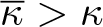 $\overline\kappa \gt \kappa$ such that
 \begin{equation*} \kappa \le k_{\varepsilon}\le \overline \kappa,\quad \forall\varepsilon\in(0,\overline\varepsilon).\end{equation*}
 On the one hand, observe that 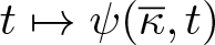 $t\mapsto \psi(\overline \kappa,t)$ is continuous and $\psi(\overline \kappa,t)\to 1-\theta \gt 0$ as t → 0, which implies that there exists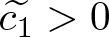 $\widetilde{c_1} \gt 0$ and $\widetilde{t} \gt 0$ such that
 \begin{equation*}
\sinh((1-\theta)\overline \kappa t)\ge \widetilde{c_1}\cdot \sinh(\overline \kappa t),\quad \forall t\in[0,\widetilde{t}].
\end{equation*}
\begin{equation*}
\sinh((1-\theta)\overline \kappa t)\ge \widetilde{c_1}\cdot \sinh(\overline \kappa t),\quad \forall t\in[0,\widetilde{t}].
\end{equation*} On the other hand, since 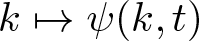 $k\mapsto \psi(k,t)$ is decreasing, the above estimate holds for every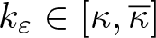 $k_\varepsilon\in[\kappa,\overline\kappa]$. Hence,
 \begin{equation*}
\sinh((1-\theta)k_{\varepsilon} t)\ge \widetilde{c_1}\cdot \sinh(k_{\varepsilon} t),\quad \forall t\in[0,\widetilde{t}], \varepsilon\in(0,\overline\varepsilon).
\end{equation*}
\begin{equation*}
\sinh((1-\theta)k_{\varepsilon} t)\ge \widetilde{c_1}\cdot \sinh(k_{\varepsilon} t),\quad \forall t\in[0,\widetilde{t}], \varepsilon\in(0,\overline\varepsilon).
\end{equation*} Now we focus on the case when  $t \gt \widetilde{t}$. Studying the asymptotic behaviour of φɛ we obtain
 \begin{equation*}
\varphi_\varepsilon(t)\ge t k_\varepsilon-\frac{\varepsilon\theta}{1-\theta}\stackrel{\textrm{def}}{=} tk_\varepsilon-s_\varepsilon,\quad \forall t \gt 0, \varepsilon\in(0,\overline\varepsilon).
\end{equation*}
\begin{equation*}
\varphi_\varepsilon(t)\ge t k_\varepsilon-\frac{\varepsilon\theta}{1-\theta}\stackrel{\textrm{def}}{=} tk_\varepsilon-s_\varepsilon,\quad \forall t \gt 0, \varepsilon\in(0,\overline\varepsilon).
\end{equation*} Note that 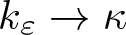 $k_\varepsilon\to\kappa$ and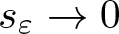 $s_\varepsilon\to0$ as ɛ → 0. Thus, since $\widetilde{t} \gt 0$, there exists an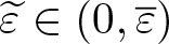 $\widetilde{\varepsilon}\in(0,\overline{\varepsilon})$ such that
 \begin{equation}
\varphi_\varepsilon(\widetilde t)\ge \widetilde{t}k_\varepsilon-s_\varepsilon \gt s_\varepsilon \gt 0,\quad \forall \varepsilon\in(0,\widetilde \varepsilon).
\end{equation}
\begin{equation}
\varphi_\varepsilon(\widetilde t)\ge \widetilde{t}k_\varepsilon-s_\varepsilon \gt s_\varepsilon \gt 0,\quad \forall \varepsilon\in(0,\widetilde \varepsilon).
\end{equation} Since 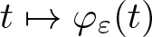 $t\mapsto \varphi_\varepsilon(t)$ is increasing, we also have
 \begin{equation}
\varphi_\varepsilon(t)\ge tk_\varepsilon-s_\varepsilon \gt s_\varepsilon \gt 0,\quad \forall \varepsilon\in(0,\widetilde \varepsilon),t \gt \widetilde{t}.
\end{equation}
\begin{equation}
\varphi_\varepsilon(t)\ge tk_\varepsilon-s_\varepsilon \gt s_\varepsilon \gt 0,\quad \forall \varepsilon\in(0,\widetilde \varepsilon),t \gt \widetilde{t}.
\end{equation}It follows that
 \begin{align*}
\sinh(\varphi_\varepsilon(t)) & \ge \sinh(tk_\varepsilon-s_\varepsilon)=\sinh(tk_\varepsilon)\cosh(s_\varepsilon)-\cosh(tk_\varepsilon)\sinh(s_\varepsilon) \\
& =\sinh(tk_\varepsilon)\cdot\left(\cosh(s_\varepsilon)-\coth(tk_\varepsilon)\sinh(s_\varepsilon)\right).
\end{align*}
\begin{align*}
\sinh(\varphi_\varepsilon(t)) & \ge \sinh(tk_\varepsilon-s_\varepsilon)=\sinh(tk_\varepsilon)\cosh(s_\varepsilon)-\cosh(tk_\varepsilon)\sinh(s_\varepsilon) \\
& =\sinh(tk_\varepsilon)\cdot\left(\cosh(s_\varepsilon)-\coth(tk_\varepsilon)\sinh(s_\varepsilon)\right).
\end{align*}Since the hyperbolic cotangent is decreasing, using relation (65), we obtain that
 \begin{align*}
\sinh(\varphi_\varepsilon(t)) & \ge \sinh(tk_\varepsilon)\cdot \left(\cosh(s_\varepsilon)-\coth(2s_\varepsilon)\sinh(s_\varepsilon)\right)= \sinh(tk_\varepsilon)\cdot \frac{1}{2\cosh(s_\varepsilon)}
\end{align*}
\begin{align*}
\sinh(\varphi_\varepsilon(t)) & \ge \sinh(tk_\varepsilon)\cdot \left(\cosh(s_\varepsilon)-\coth(2s_\varepsilon)\sinh(s_\varepsilon)\right)= \sinh(tk_\varepsilon)\cdot \frac{1}{2\cosh(s_\varepsilon)}
\end{align*} Define 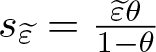 $s_{\widetilde{\varepsilon}}=\frac{\widetilde{\varepsilon}\theta}{1-\theta}$, the monotonicity of the hyperbolic cosine implies
 \begin{align*}
\sinh(\varphi_\varepsilon(t)) & \ge \sinh(tk_\varepsilon)\cdot \frac{1}{2\cosh(s_{\widetilde{\varepsilon}})}\stackrel{\textrm{def}}{=} \widetilde{c_2}\cdot \sinh(tk_\varepsilon).
\end{align*}
\begin{align*}
\sinh(\varphi_\varepsilon(t)) & \ge \sinh(tk_\varepsilon)\cdot \frac{1}{2\cosh(s_{\widetilde{\varepsilon}})}\stackrel{\textrm{def}}{=} \widetilde{c_2}\cdot \sinh(tk_\varepsilon).
\end{align*} Thus,  $\widetilde{c}=\min\{\widetilde{c_1},\widetilde{c_2}\}$ and $\widetilde{\varepsilon}$ yield inequality (63), for every $t\ge 0$.
Combining the above estimates, we obtain for every  $t\ge 0$ and $0 \lt \varepsilon \lt \widetilde{\varepsilon}$ that
 \begin{align}
& c \sinh(k_\varepsilon t)^{n-1}\stackrel{\textrm{def}}{=} \frac{(1-\theta^2)^\frac{n+1}{2}(\widetilde{c})^{n-1}}{\vartheta_{\varepsilon}^{n-1}}\sinh(k_\varepsilon t)^{n-1} \le \psi_\varepsilon(t)\nonumber\\ & \quad \le \frac{k_\varepsilon}{\vartheta^n}\sinh(k_\varepsilon t)^{n-1}\stackrel{\textrm{def}}{=} C \sinh(k_\varepsilon t)^{n-1}.
\end{align}
\begin{align}
& c \sinh(k_\varepsilon t)^{n-1}\stackrel{\textrm{def}}{=} \frac{(1-\theta^2)^\frac{n+1}{2}(\widetilde{c})^{n-1}}{\vartheta_{\varepsilon}^{n-1}}\sinh(k_\varepsilon t)^{n-1} \le \psi_\varepsilon(t)\nonumber\\ & \quad \le \frac{k_\varepsilon}{\vartheta^n}\sinh(k_\varepsilon t)^{n-1}\stackrel{\textrm{def}}{=} C \sinh(k_\varepsilon t)^{n-1}.
\end{align} Since v is positive and decreasing, the positive homogeneity of  $F^*_\varepsilon$ and the relations from (61) imply
 \begin{equation}
F^*_\varepsilon(Du^\star_{\varepsilon,T})=F^*_\varepsilon(v_{\varepsilon,T}'(\rho_\varepsilon)D\rho_\varepsilon)=\begin{cases}
\frac{v(t_2)}{t_2-t_1}F^*_\varepsilon(D\rho_\varepsilon), & \text{if } \rho_\varepsilon\in(t_1,t_2), \\
|v'(\rho_\varepsilon)|F^*_\varepsilon(-D\rho_\varepsilon) & \text{if } \rho_\varepsilon\in(t_2,t_3), \\
\frac{v(t_3)}{t_4-t_3}F^*_\varepsilon(-D\rho_\varepsilon) & \text{if } \rho_\varepsilon\in(t_3,t_4), \\
0, & \text{if }\rho_\varepsilon\in(0,t_1)\cup(t_4,R).
\end{cases}
\end{equation}
\begin{equation}
F^*_\varepsilon(Du^\star_{\varepsilon,T})=F^*_\varepsilon(v_{\varepsilon,T}'(\rho_\varepsilon)D\rho_\varepsilon)=\begin{cases}
\frac{v(t_2)}{t_2-t_1}F^*_\varepsilon(D\rho_\varepsilon), & \text{if } \rho_\varepsilon\in(t_1,t_2), \\
|v'(\rho_\varepsilon)|F^*_\varepsilon(-D\rho_\varepsilon) & \text{if } \rho_\varepsilon\in(t_2,t_3), \\
\frac{v(t_3)}{t_4-t_3}F^*_\varepsilon(-D\rho_\varepsilon) & \text{if } \rho_\varepsilon\in(t_3,t_4), \\
0, & \text{if }\rho_\varepsilon\in(0,t_1)\cup(t_4,R).
\end{cases}
\end{equation}According to remark 5.2(d), one has
 \begin{align*}& F^*_\varepsilon(D\rho_\varepsilon)=1,\quad\mbox{and}\quad F^*_\varepsilon(-D\rho_\varepsilon)=\frac{1-\frac{\overline{r}(\overline{r}+2\varepsilon)}{(\overline{r}+\varepsilon)^2}\theta}{1+\frac{\overline{r}(\overline{r}+2\varepsilon)}{(\overline{r}+\varepsilon)^2}\theta}\stackrel{\textrm{def}}{=} h_\varepsilon(\overline{r}),\nonumber\\ & \quad\mbox{where}\quad \frac{1-\theta}{1+\theta}\le h_\varepsilon(\overline{r})\le1.\end{align*}
 Observe that  $h_\varepsilon(\overline{r})$ is decreasing in $ \overline{r}$, increasing in ɛ, and approaches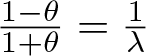 $\frac{1-\theta}{1+\theta}=\frac{1}{\lambda}$ as ɛ → 0. Clearly one has
 \begin{equation*}\overline r=\varphi_\varepsilon(t)\ge (1-\theta)k_\varepsilon t\ge(1-\theta)\kappa t,\end{equation*}
thus, we also obtain
 \begin{equation}
h_\varepsilon(\overline{r})=h_\varepsilon(\varphi_\varepsilon(t))\le h_\varepsilon((1-\theta)\kappa t)\le 1.
\end{equation}
\begin{equation}
h_\varepsilon(\overline{r})=h_\varepsilon(\varphi_\varepsilon(t))\le h_\varepsilon((1-\theta)\kappa t)\le 1.
\end{equation}As before, denote by ω the volume of the Euclidean unit ball of dimension n.
On the one hand, relations (62) and (67) yield
 \begin{align*}
I
& =\frac{v(t_2)^p}{(t_2-t_1)^p}\int_{t_1}^{t_2} w(t) \psi_\varepsilon(t)e(t)\,\mathrm{d} t + \int_{t_2}^{t_3} w(t)|v'(t)|^p h_\varepsilon^p(\varphi_\varepsilon(t)) \psi_\varepsilon(t)e(t)\,\mathrm{d} t
\\
& \qquad +\frac{v(t_3)^p}{(t_4-t_3)^p}\int_{t_3}^{t_4} w(t) h_\varepsilon^p(\varphi_\varepsilon(t))\psi_\varepsilon(t)e(t)\,\mathrm{d} t.
\end{align*}
\begin{align*}
I
& =\frac{v(t_2)^p}{(t_2-t_1)^p}\int_{t_1}^{t_2} w(t) \psi_\varepsilon(t)e(t)\,\mathrm{d} t + \int_{t_2}^{t_3} w(t)|v'(t)|^p h_\varepsilon^p(\varphi_\varepsilon(t)) \psi_\varepsilon(t)e(t)\,\mathrm{d} t
\\
& \qquad +\frac{v(t_3)^p}{(t_4-t_3)^p}\int_{t_3}^{t_4} w(t) h_\varepsilon^p(\varphi_\varepsilon(t))\psi_\varepsilon(t)e(t)\,\mathrm{d} t.
\end{align*} Applying relations (66), (68), and using the definition of  $\mathcal{I}^{k,h}$ from (60), we obtain
 \begin{align*}
I
& \le \frac{v(t_2)^p}{(t_2-t_1)^p}\int_{t_1}^{t_2} w(t) \psi_\varepsilon(t)e(t)\,\mathrm{d} t+ \int_{t_2}^{t_3} w(t)|v'(t)|^p h_\varepsilon^p((1-\theta)\kappa t) \psi_\varepsilon(t)e(t)\,\mathrm{d} t \\
& \qquad +\frac{v(t_3)^p}{(t_4-t_3)^p}\int_{t_3}^{t_4} w(t) h_\varepsilon^p((1-\theta)\kappa t)\psi_\varepsilon(t)e(t)\,\mathrm{d} t
\\ &\le \frac{Cv(t_2)^p}{(t_2-t_1)^p}\int_{t_1}^{t_2} w(t) \sinh(k_\varepsilon t)^{n-1}e(t)\,\mathrm{d} t+ h_\varepsilon^p((1-\theta)\kappa t_2)\int_{t_2}^{t_3} w(t)|v'(t)|^p \psi_\varepsilon(t)e(t)\,\mathrm{d} t \\
& \qquad +\frac{C h_\varepsilon^p((1-\theta)\kappa t_3)v(t_3)^p}{(t_4-t_3)^p}\int_{t_3}^{t_4} w(t)\sinh(k_\varepsilon t)^{n-1}e(t)\,\mathrm{d} t \\
& \le \frac{Cv(t_2)^p\cdot \mathcal{I}^{k_\varepsilon,h}(w;t_1,t_2)}{(t_2-t_1)^p} + h_\varepsilon^p((1-\theta)\kappa t_2)\int_{t_2}^{t_3} w(t)|v'(t)|^p \psi_\varepsilon(t)e(t)\,\mathrm{d} t \\ & \quad +\frac{C v(t_3)^p\cdot\mathcal{I}^{k_\varepsilon,h}(w;t_3,t_4)}{(t_4-t_3)^p}.
\end{align*}
\begin{align*}
I
& \le \frac{v(t_2)^p}{(t_2-t_1)^p}\int_{t_1}^{t_2} w(t) \psi_\varepsilon(t)e(t)\,\mathrm{d} t+ \int_{t_2}^{t_3} w(t)|v'(t)|^p h_\varepsilon^p((1-\theta)\kappa t) \psi_\varepsilon(t)e(t)\,\mathrm{d} t \\
& \qquad +\frac{v(t_3)^p}{(t_4-t_3)^p}\int_{t_3}^{t_4} w(t) h_\varepsilon^p((1-\theta)\kappa t)\psi_\varepsilon(t)e(t)\,\mathrm{d} t
\\ &\le \frac{Cv(t_2)^p}{(t_2-t_1)^p}\int_{t_1}^{t_2} w(t) \sinh(k_\varepsilon t)^{n-1}e(t)\,\mathrm{d} t+ h_\varepsilon^p((1-\theta)\kappa t_2)\int_{t_2}^{t_3} w(t)|v'(t)|^p \psi_\varepsilon(t)e(t)\,\mathrm{d} t \\
& \qquad +\frac{C h_\varepsilon^p((1-\theta)\kappa t_3)v(t_3)^p}{(t_4-t_3)^p}\int_{t_3}^{t_4} w(t)\sinh(k_\varepsilon t)^{n-1}e(t)\,\mathrm{d} t \\
& \le \frac{Cv(t_2)^p\cdot \mathcal{I}^{k_\varepsilon,h}(w;t_1,t_2)}{(t_2-t_1)^p} + h_\varepsilon^p((1-\theta)\kappa t_2)\int_{t_2}^{t_3} w(t)|v'(t)|^p \psi_\varepsilon(t)e(t)\,\mathrm{d} t \\ & \quad +\frac{C v(t_3)^p\cdot\mathcal{I}^{k_\varepsilon,h}(w;t_3,t_4)}{(t_4-t_3)^p}.
\end{align*} By relation (59), for every 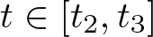 $t\in[t_2,t_3]$ one has
 \begin{equation*}
\frac{1}{W(t)}\left|\frac{v'(t)}{v(t)}\right|^p=\frac{1}{W(t)}\left(-\frac{v'(t)}{v(t)}\right)^p=\frac{G(t)^{p'}}{W(t)}.
\end{equation*}
\begin{equation*}
\frac{1}{W(t)}\left|\frac{v'(t)}{v(t)}\right|^p=\frac{1}{W(t)}\left(-\frac{v'(t)}{v(t)}\right)^p=\frac{G(t)^{p'}}{W(t)}.
\end{equation*} The above function is continuous, thus, it attains it maximum on 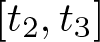 $[t_2,t_3]$, hence we have
 \begin{align*}
\int_{t_2}^{t_3} w(t)|v'(t)|^p \psi_\varepsilon(t)\,\mathrm{d} t&=\int_{t_2}^{t_3} \frac{1}{W(t)}\left|\frac{v'(t)}{v(t)}\right|^p w(t) W(t)(v(t))^p \psi_\varepsilon(t)\,\mathrm{d} t\\
&\le \max_{t\in[t_2,t_3]} \frac{G(t)^{p'}}{W(t)}\cdot \int_{t_2}^{t_3} w(t) W(t) (v(t))^p \psi_\varepsilon(t)e(t)\,\mathrm{d} t.
\end{align*}
\begin{align*}
\int_{t_2}^{t_3} w(t)|v'(t)|^p \psi_\varepsilon(t)\,\mathrm{d} t&=\int_{t_2}^{t_3} \frac{1}{W(t)}\left|\frac{v'(t)}{v(t)}\right|^p w(t) W(t)(v(t))^p \psi_\varepsilon(t)\,\mathrm{d} t\\
&\le \max_{t\in[t_2,t_3]} \frac{G(t)^{p'}}{W(t)}\cdot \int_{t_2}^{t_3} w(t) W(t) (v(t))^p \psi_\varepsilon(t)e(t)\,\mathrm{d} t.
\end{align*}On the other hand, we obtain
 \begin{align}
J& =\int_{0}^{R} w(t) W(t) (v_{\varepsilon,T}(t))^p \psi_\varepsilon(t)e(t)\,\mathrm{d} t
\ge \int_{t_2}^{t_3} w(t) W(t) (v(t))^p \psi_\varepsilon(t)e(t)\,\mathrm{d} t \nonumber\\ & \ge c\cdot \mathcal{I}^{k_\varepsilon,h}(wW v^p;t_2,t_3).
\end{align}
\begin{align}
J& =\int_{0}^{R} w(t) W(t) (v_{\varepsilon,T}(t))^p \psi_\varepsilon(t)e(t)\,\mathrm{d} t
\ge \int_{t_2}^{t_3} w(t) W(t) (v(t))^p \psi_\varepsilon(t)e(t)\,\mathrm{d} t \nonumber\\ & \ge c\cdot \mathcal{I}^{k_\varepsilon,h}(wW v^p;t_2,t_3).
\end{align}Combining the above results and using both inequalities of (69), it follows that
 \begin{align*}
\frac{\lambda^p I}{J}
& \le \lambda^p h_\varepsilon^p((1-\theta)\kappa t_2)\cdot \max_{t\in[t_2,t_3]} \frac{G(t)^{p'}}{W(t)} \\
& \qquad +\frac{\lambda^p C}{c}\left(\frac{v(t_2)^p\cdot \mathcal{I}^{k_\varepsilon,h}(w;t_1,t_2)}{(t_2-t_1)^p\cdot \mathcal{I}^{k_\varepsilon,h}(wW v^p;t_2,t_3)}+\frac{v(t_3)^p\cdot \mathcal{I}^{k_\varepsilon,h}(w;t_3,t_4)}{(t_4-t_3)^p\cdot \mathcal{I}^{k_\varepsilon,h}(wW v^p;t_2,t_3)}\right) \\
& =\lambda^p\cdot (l_2^{k_\varepsilon,h}(\delta))^p\cdot l_1^{k_\varepsilon,h}(\delta)+\frac{\lambda^p C}{c}\cdot l_0^{k_\varepsilon,h}(\delta).
\end{align*}
\begin{align*}
\frac{\lambda^p I}{J}
& \le \lambda^p h_\varepsilon^p((1-\theta)\kappa t_2)\cdot \max_{t\in[t_2,t_3]} \frac{G(t)^{p'}}{W(t)} \\
& \qquad +\frac{\lambda^p C}{c}\left(\frac{v(t_2)^p\cdot \mathcal{I}^{k_\varepsilon,h}(w;t_1,t_2)}{(t_2-t_1)^p\cdot \mathcal{I}^{k_\varepsilon,h}(wW v^p;t_2,t_3)}+\frac{v(t_3)^p\cdot \mathcal{I}^{k_\varepsilon,h}(w;t_3,t_4)}{(t_4-t_3)^p\cdot \mathcal{I}^{k_\varepsilon,h}(wW v^p;t_2,t_3)}\right) \\
& =\lambda^p\cdot (l_2^{k_\varepsilon,h}(\delta))^p\cdot l_1^{k_\varepsilon,h}(\delta)+\frac{\lambda^p C}{c}\cdot l_0^{k_\varepsilon,h}(\delta).
\end{align*} By our assumptions, the last relation approaches 1 as 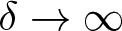 $\delta\to\infty$, thus, the inequality (58) is sharp on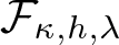 $\mathcal{F}_{\kappa,h,\lambda}$.
Observe that in contrast with theorem 4.3, the limits appearing in the statement of the above result are strongly dependent on ɛ. The reason for this stems from the observation of remark 5.2(a): Since the flag curvature is not increasing along  $\nabla\rho$, we need to work with kɛ instead of κ, which explains the dependence on ɛ. Fortunately, by suitable choices of $\varepsilon(\delta)$, one can provide sharpness results in this setting, as well. Such an example is presented in the sequel.
5.3. The sharpness of a McKean-type spectral gap estimate
In this section, we prove a sharpness result concerning a McKean-type spectral gap estimate on 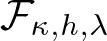 $\mathcal{F}_{\kappa,h,\lambda}$ (which for p = 2 reduces to theorem 1.2). Our last result can be stated as follows.
Theorem 5.4. Let  $n\ge 2$, $\lambda,p\in (1,\infty)$, and $\kappa \gt h\ge0$. For every $(\mathbb{B}^n,F_\varepsilon,\mathsf{m}_\varepsilon)\in \mathcal{F}_{\kappa,h,\lambda}$ and $u\in C_0^\infty(\mathbb{B}^n)$ one has
 \begin{align}
\lambda^p\displaystyle\int_{\mathbb{B}^n} F_\varepsilon^*(Du)^p\,\mathrm{d} \mathsf{m}_\varepsilon\ge c_{n,p,\kappa,h}\int_{\mathbb{B}^n} |u|^p \,\mathrm{d} \mathsf{m}_\varepsilon,\quad\text{where}\quad c_{n,p,\kappa,h}=\left(\frac{(n-1)(\kappa-h)}{p}\right)^p.
\end{align}
\begin{align}
\lambda^p\displaystyle\int_{\mathbb{B}^n} F_\varepsilon^*(Du)^p\,\mathrm{d} \mathsf{m}_\varepsilon\ge c_{n,p,\kappa,h}\int_{\mathbb{B}^n} |u|^p \,\mathrm{d} \mathsf{m}_\varepsilon,\quad\text{where}\quad c_{n,p,\kappa,h}=\left(\frac{(n-1)(\kappa-h)}{p}\right)^p.
\end{align} Moreover, 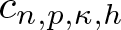 $c_{n,p,\kappa,h}$ is sharp in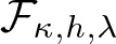 $\mathcal{F}_{\kappa,h,\lambda}$, in the sense that it is the greatest constant with this property.
Proof. The validity of inequality (70) follows from theorem 3.4. To prove the sharpness, we use theorem 5.3. Recall the definition of  $\widetilde\varepsilon$ from (64). Let δ > 1, such that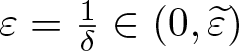 $\varepsilon=\frac{1}{\delta}\in(0,\widetilde\varepsilon)$, and define
 \begin{equation*}
t_1(\delta)=\delta,\quad
t_2(\delta)=2\delta,\quad
t_3(\delta)=3\delta,\quad\mbox{and}\quad
t_4(\delta)=4\delta.
\end{equation*}
\begin{equation*}
t_1(\delta)=\delta,\quad
t_2(\delta)=2\delta,\quad
t_3(\delta)=3\delta,\quad\mbox{and}\quad
t_4(\delta)=4\delta.
\end{equation*}By a simple computation, we obtain
 \begin{align*}l_2^{k_\varepsilon,h}& =h_\varepsilon((1-\theta)\kappa t_2)=\frac{1+4\delta^2(1-\theta)^2\kappa+4\delta^4(1-\theta)^3\kappa^2}{1+4\delta^2(1-\theta^2)\kappa+4\delta^4(1-\theta)^2(1+\theta)\kappa^2}\nonumber\\ & \quad \to \frac{1-\theta}{1+\theta}=\lambda,\quad\text{as}\quad \delta\to \infty.\end{align*}
Consider the following functions (see also the proof of theorem 3.4):
 \begin{align*}
w(t)= 1,
\quad W(t)& =c_{n,p,\kappa,h},
\quad G(t)\equiv (c_{n,p,\kappa,h})^\frac{p-1}{p},\quad\mbox{and}\quad v(t)^p=e^{-(n-1)t (\kappa-h)},\nonumber\\ & \forall t \gt 0.
\end{align*}
\begin{align*}
w(t)= 1,
\quad W(t)& =c_{n,p,\kappa,h},
\quad G(t)\equiv (c_{n,p,\kappa,h})^\frac{p-1}{p},\quad\mbox{and}\quad v(t)^p=e^{-(n-1)t (\kappa-h)},\nonumber\\ & \forall t \gt 0.
\end{align*} Since  $k_\varepsilon \gt \kappa \gt h$, the following expressions are strictly increasing in t:
 \begin{align*}
w(t)\sinh(k_\varepsilon t)^{n-1}e^{-(n-1)h t} & = \sinh(k_\varepsilon t)^{n-1}e^{-(n-1)h t}, \\
w(t)W(t)v(t)^p\sinh(k_\varepsilon t)^{n-1}e^{-(n-1)h t} & =c_{n,p,\kappa,h}\sinh(k_\varepsilon t)^{n-1}e^{-(n-1)\kappa t}.
\end{align*}
\begin{align*}
w(t)\sinh(k_\varepsilon t)^{n-1}e^{-(n-1)h t} & = \sinh(k_\varepsilon t)^{n-1}e^{-(n-1)h t}, \\
w(t)W(t)v(t)^p\sinh(k_\varepsilon t)^{n-1}e^{-(n-1)h t} & =c_{n,p,\kappa,h}\sinh(k_\varepsilon t)^{n-1}e^{-(n-1)\kappa t}.
\end{align*}On the one hand, we have
 \begin{align*}
\frac{v(t_2)^p\cdot\mathcal{I}^{k_\varepsilon,h}(w;t_1,t_2)}{(t_2-t_1)^p\cdot \mathcal{I}^{k_\varepsilon,h}(wWv^p;t_2,t_3)}
& \le \frac{v(t_2)^p}{(t_2-t_1)^p}\cdot \frac{(t_2-t_1)\sinh(k_\varepsilon t_1)^{n-1} e^{-(n-1)ht_1}}{(t_3-t_2)c_{n,p,\kappa,h}\sinh(k_\varepsilon t_3)^{n-1}e^{-(n-1)h t_3}} \\
& =\frac{e^{(n-1)\delta(\kappa+h)}\sinh(\delta k_\varepsilon)^{n-1}}{\delta^pc_{n,p,\kappa,h} \sinh(3\delta k_\varepsilon)^{n-1}}\\
&= \frac{e^{(n-1)\delta(\kappa+h-2k_\varepsilon)}}{\delta^pc_{n,p,\kappa,h}}\cdot \frac{e^{(n-1)\delta(2k_\varepsilon)}\sinh(\delta k_\varepsilon)^{n-1}}{\sinh(3\delta k_\varepsilon)^{n-1}}\\
& \quad \to 0\cdot 1=0, \quad\text{as}\quad \delta\to\infty.
\end{align*}
\begin{align*}
\frac{v(t_2)^p\cdot\mathcal{I}^{k_\varepsilon,h}(w;t_1,t_2)}{(t_2-t_1)^p\cdot \mathcal{I}^{k_\varepsilon,h}(wWv^p;t_2,t_3)}
& \le \frac{v(t_2)^p}{(t_2-t_1)^p}\cdot \frac{(t_2-t_1)\sinh(k_\varepsilon t_1)^{n-1} e^{-(n-1)ht_1}}{(t_3-t_2)c_{n,p,\kappa,h}\sinh(k_\varepsilon t_3)^{n-1}e^{-(n-1)h t_3}} \\
& =\frac{e^{(n-1)\delta(\kappa+h)}\sinh(\delta k_\varepsilon)^{n-1}}{\delta^pc_{n,p,\kappa,h} \sinh(3\delta k_\varepsilon)^{n-1}}\\
&= \frac{e^{(n-1)\delta(\kappa+h-2k_\varepsilon)}}{\delta^pc_{n,p,\kappa,h}}\cdot \frac{e^{(n-1)\delta(2k_\varepsilon)}\sinh(\delta k_\varepsilon)^{n-1}}{\sinh(3\delta k_\varepsilon)^{n-1}}\\
& \quad \to 0\cdot 1=0, \quad\text{as}\quad \delta\to\infty.
\end{align*}On the other hand, observe that
 \begin{align*}
\frac{v(t_3)^p\cdot\mathcal{I}^{k_\varepsilon,h}(w;t_3,t_4)}{(t_4-t_3)^p\cdot \mathcal{I}^{k_\varepsilon,h}(wWv^p;t_2,t_3)}
&\le \frac{v(t_3)^p}{(t_4-t_3)^p}\cdot \frac{(t_4-t_3)\sinh(\kappa t_3)^{n-1} e^{-(n-1)ht_3}}{(t_3-t_2)c_{n,p,\kappa,h}\sinh(\kappa t_3)^{n-1}e^{-(n-1)\kappa t_3}} \\
&=\frac{1}{\delta^pc_{n,p,\kappa,h} }\to 0,\quad\mbox{as }\delta\to\infty.
\end{align*}
\begin{align*}
\frac{v(t_3)^p\cdot\mathcal{I}^{k_\varepsilon,h}(w;t_3,t_4)}{(t_4-t_3)^p\cdot \mathcal{I}^{k_\varepsilon,h}(wWv^p;t_2,t_3)}
&\le \frac{v(t_3)^p}{(t_4-t_3)^p}\cdot \frac{(t_4-t_3)\sinh(\kappa t_3)^{n-1} e^{-(n-1)ht_3}}{(t_3-t_2)c_{n,p,\kappa,h}\sinh(\kappa t_3)^{n-1}e^{-(n-1)\kappa t_3}} \\
&=\frac{1}{\delta^pc_{n,p,\kappa,h} }\to 0,\quad\mbox{as }\delta\to\infty.
\end{align*} Combining the above two limits, we obtain 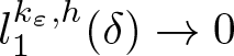 $l_1^{k_\varepsilon,h}(\delta)\to 0$ as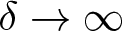 $\delta\to\infty$.
Finally, since
 \begin{equation*}
\frac{G(t)^{p'}}{W(t)}=1, \quad\forall t \gt 0,
\end{equation*}
\begin{equation*}
\frac{G(t)^{p'}}{W(t)}=1, \quad\forall t \gt 0,
\end{equation*} we also obtain 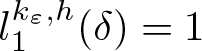 $l_1^{k_\varepsilon,h}(\delta)=1$. Thus, theorem 5.3 yields the sharpness of the inequality (70), which concludes the paper.
Acknowledgements
The author would like to thank Prof. Alexandru Kristály for the valuable discussions on the subject of the paper. He is also grateful to the anonymous reviewer for carefully reading the article and providing valuable comments.
Funding statement
The author is supported by the János Bolyai Research Scholarship of the Hungarian Academy of Sciences.
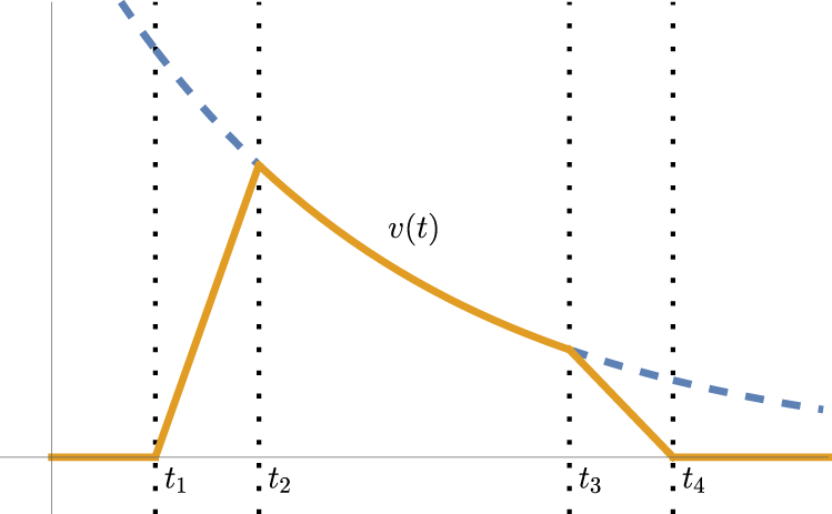


 Open access

