


1. Introduction
The controlled steering of microscale and nanoscale objects in fluidic environments by external driving has received significant attention in recent years as an emergent topic of ‘driven matter’ in physics (Witten & Diamant Reference Witten and Diamant2020) and due to their prospective biomedical applications, such as targeted drug delivery and microsurgery (Li et al. Reference Li, de Á vila, Zhang and Wang2017; Wang et al. Reference Wang, Kostarelos, Nelson and Zhang2021; Ruiz-González et al. Reference Ruiz-González, Esporrín-Ubieto, Kim, Wang and Sánchez2025). Among the array of actuation mechanisms, magnetic-field-driven steering of microbots is one of the extensively studied techniques for in vivo applications (Zhou et al. Reference Zhou, Mayorga-Martinez, Pané, Zhang and Pumera2021; Oral & Pumera Reference Oral and Pumera2023). The conventional technique employs the magnetic field gradient, which applies a force on magnetic colloids; typically this method requires strong (tesla) fields to generate appreciable gradient over the size of the colloidal particle for its efficient steering. An alternative methodology (Ghosh & Fischer Reference Ghosh and Fischer2009; Zhang et al. Reference Zhang, Abbott, Dong, Kratochvil, Bell and Nelson2009) employs steering driven by a weak (millitesla) uniform rotating magnetic field. This approach enables efficient steering of shaped magnetic micromotors and relies on viscous rotation–translation coupling. A most obvious choice of the propeller geometry is inspired by the helical bacterial flagellum, which enables bacterial mobility through efficient rotation–translation coupling due to its geometric chirality (Berg Reference Berg2003; Lauga & Powers Reference Lauga and Powers2009). Similarly to bacteria propelled by a rotating flagellum, the magnetic microhelix rotates and propels due to the magnetic torque applied by the rotating magnetic field.
Various fabrication methodologies, including the ‘top-down’ approach (Zhang et al. Reference Zhang, Abbott, Dong, Kratochvil, Bell and Nelson2009), glancing angle deposition (Ghosh & Fischer Reference Ghosh and Fischer2009), delamination of magnetic stripes (Smith et al. Reference Smith, Makarov, Sanchez, Fomin and Schmidt2011), direct laser writing (Tottori et al. Reference Tottori, Zhang, Qiu, Krawczyk, Franco-Obregón and Nelson2012), template-assisted deposition (Li et al. Reference Li, Sattayasamitsathit, Dong, Gao, Tam, Feng, Ai and Wang2014), biotemplating (Gao et al. Reference Gao, Feng, Pei, Kane, Tam, Hennessy and Wang2014; Yan et al. Reference Yan2015), photopolymerization of magnetic polymer composites (Peters et al. Reference Peters, Ergeneman, Nelson and Hierold2013) and spiralling microfluidic flow lithography (Yu et al. Reference Yu, Shang, Gao, Zhao, Wang and Zhao2017), have been developed for fabricating magnetic microhelices. The obvious bioinspired design of microhelices was later extended to simpler geometrically achiral planar (two-dimensional) micropropellers (Cheang et al. Reference Cheang, Meshkati, Kim, Kim and Fu2014), which can be mass-fabricated using photolithography (Tottori & Nelson Reference Tottori and Nelson2018; Duygu et al. Reference Duygu, Cheang, Leshansky and Kim2024), flexible (one-dimensional) magnetic nanowires that acquire shape requited for rotation–translation coupling dynamically due to the competition of viscous and elastic forces (Gao et al. Reference Gao, Sattayasamitsathit, Manesh, Weihs and Wang2010; Pak et al. Reference Pak, Gao, Wang and Lauga2011), and spontaneously aggregated clusters of magnetic nanoparticles (Vach et al. Reference Vach, Brun, Bennet, Bertinetti, Widdrat, Baumgartner, Klumpp, Fratzl and Faivre2013, Reference Vach, Fratzl, Klumpp and Faivre2015) exhibiting random shape anisotropy.
Most previous theoretical and computational studies focused almost exclusively on driven dynamics of non-Brownian magnetic microbots, including actuation regimes (i.e. synchronous versus asynchronous), the role of geometry (e.g. chiral, achiral or random shaped) and magnetization orientation, types of magnetization (i.e. permanently magnetized versus magnetically polarizable), configuration of the actuating field (i.e. uniform and amplitude-modulated in-plane rotating, conically rotating, etc.), collective dynamics and other topics (see the recent review Pumera et al. (Reference Pumera2025) for details). In particular, the dynamics of a slender ferromagnetic microhelix in a viscous liquid driven by the uniform in-plane rotating magnetic field was first studied by Ghosh et al. (Reference Ghosh, Mandal, Karmakar and Ghosh2013) and Morozov & Leshansky (Reference Morozov and Leshansky2014a ) assuming cylindrical rotational anisotropy. The analogous theory for magnetically polarizable (i.e. superparamagnetic) microhelices (e.g. Peters et al. Reference Peters, Ergeneman, Nelson and Hierold2013) was developed by Morozov & Leshansky (Reference Morozov and Leshansky2014b ). Later Morozov et al. (Reference Morozov, Mirzae, Kenneth and Leshansky2017) developed a general hydrodynamic theory for the torque-driven actuation of arbitrarily shaped and magnetized propeller, establishing the dependence of its dynamic orientation and propulsion on the geometry and magnetization; the theory was recently extended to arbitrary superparamagnetic microbots (Morozov et al. Reference Morozov, Zusmanovich, Rubinstein and Leshansky2025). This general theory confirmed the experimental observations for a propeller made from three interconnected magnetic microbeads (Cheang et al. Reference Cheang, Meshkati, Kim, Kim and Fu2014) and showed that depending on orientation of the magnetic dipolar moment, individual geometrically achiral objects exhibit net propulsion. In particular, it was demonstrated that magnetization of the three-bead propeller in the plane of the beads’ centres resulted in bidirectional propulsion, whereas individual propellers can move in diametrically opposite directions (i.e. parallel and antiparallel to the field rotation axis) with equal speeds. It was also predicted that a specific off-plane magnetization yields unidirectional propulsion of the three-bead propeller, being typically associated with geometrically chiral (e.g. helical) propellers. Notice that the fastest random computer-generated magnetic clusters actually resembled a planar arc, rather than a helix (Mirzae et al. Reference Mirzae, Dubrovski, Kenneth, Morozov and Leshansky2018). Moreover, geometric optimization revealed that the optimal planar propellers are arc-shaped and they fall short (approximately 30 %) of the optimal three-dimensional structures with skew symmetry (Mirzae et al. Reference Mirzae, Dubrovski, Kenneth, Morozov and Leshansky2018). A formal symmetry analysis (involving parity and charge conjugation) was put forward by Sachs et al. (Reference Sachs, Morozov, Kenneth, Qiu, Segreto, Fischer and Leshansky2018) to establish a correspondence between the magnetization orientation and propulsion gaits of torque-driven microbots. In particular, it was predicted that a symmetric two-dimensional propeller magnetized along either of the principal rotation axes exhibits no net propulsion. Individual less symmetric in-plane magnetized microbots exhibit bidirectional propulsion due to a spontaneous symmetry breaking, so that their ensemble average velocity vanishes. Off-plane magnetization can render the symmetric V-shape propeller chiral, whereas the intrinsically broken symmetry results in its unidirectional motion. These theoretical predictions were supported by experiments with a 3D-printed (centimetre-sized) arc-shaped propeller and microscopic V-shaped microbots driven by a rotating magnetic (and electric) field (Sachs et al. Reference Sachs, Morozov, Kenneth, Qiu, Segreto, Fischer and Leshansky2018). In reality, planar magnetic microbots (e.g. fabricated by photolithography) are prone to magnetize in their own plane, leading to bidirectional propulsion, posing a limitation on the controllable steering of their swarms. However, it was predicted theoretically (Cohen et al. Reference Cohen, Rubinstein, Kenneth and Leshansky2019) and confirmed experimentally (Duygu et al. Reference Duygu, Cheang, Leshansky and Kim2024), that adding a static magnetic field component along the field rotation axis reduces the symmetry of the problem, resulting in unidirectional propulsion of highly symmetrical planar and in-plane magnetized microbots. Similarly, adding a static field component perpendicular to the field rotation axis, results in propulsion accompanied by a net drift in plane of the field (Morozov & Leshansky Reference Morozov and Leshansky2020).
Although the above theories concern actuation and propulsion of non-Brownian microbots, current microfabrication techniques (such as ‘glancing angle deposition’) can be readily used to fabricate magnetic nanobots capable of steering through submicrometre interstitial spaces of crowded biomimetic (Schamel et al. Reference Schamel, Mark, Gibbs, Miksch, Morozov, Leshansky and Fischer2014) or biological (Dasgupta et al. Reference Dasgupta, Pally, Saini, Bhat and Ghosh2020) environments and even navigate within living biological cells (Pal et al. Reference Pal, Somalwar, Singh, Bhat, Eswarappa, Saini and Ghosh2018). At submicron scale, thermal noise becomes increasingly significant, and may become comparable in magnitude to the magnetic driving, thereby hindering the actuation and impairing propulsion. This raises an important question: How small a nanopropeller can be? Despite growing experimental interest in achieving controllable propulsion at nanoscale and a few previous ad hoc efforts to address this question qualitatively (Schamel et al. Reference Schamel, Mark, Gibbs, Miksch, Morozov, Leshansky and Fischer2014; Ghosh et al. Reference Ghosh, Paria, Rangarajan and Ghosh2014), a rigorous quantitative investigation of the role of thermal fluctuations on magnetically driven actuation and propulsion of magnetic nanobots was still lacking. It is also worth mentioning that this question is showing on top of the list of 10 most critical problems for the advancement of micro/nanorobots in the next decade, ‘serving as a foundation for a technology roadmap’ (Pumera et al. Reference Pumera2025).
The present paper aims to study the impact of thermal noise on torque-driven actuation and propulsion of magnetic nanohelices in a viscous fluid using numerical simulations of the Langevin equation and Fokker–Planck theory. At the nanoscale the general theoretical formalism of ‘fluctuating hydrodynamics’ reduces to a classical Langevin equation, provided that the Brownian particle is much larger compared with the fluid particle (Hauge & Martin-Löf Reference Hauge and Martin-Löf1973), and implying that the dynamics of the magnetic Brownian nanobot is governed by Stokes hydrodynamics, whereby the viscous and thermal forces and torques are counterbalanced by external forcing. The relative importance of the magnetic driving with respect to thermal noise is measured by the rotational Péclet number, $ \textit{Pe} = \textit{mH}/(k_{B} T)$
(otherwise known as Langevin parameter,
$ \textit{Pe} = \textit{mH}/(k_{B} T)$
(otherwise known as Langevin parameter, $\xi$
), where
$\xi$
), where $k_{B}$
is the Boltzmann constant,
$k_{B}$
is the Boltzmann constant, $T$
is the temperature,
$T$
is the temperature, $H$
stands for the magnitude of the rotating field and
$H$
stands for the magnitude of the rotating field and $m$
for the magnetic moment of the propeller. Qualitatively speaking, the thermal noise affects the dynamics of the torque-driven nanobot in three distinct ways: (i) by impeding its forced rotations, thereby reducing its angular velocity; (ii) perturbing its steady orientation with respect to the actuating field; (iii) obstructing its linear motion (i.e. propulsion) (Schamel et al. Reference Schamel, Mark, Gibbs, Miksch, Morozov, Leshansky and Fischer2014). The first two mechanisms rely on rotational diffusion about the propellers’ long and short axes, whereas the third mechanism stems from translational diffusion.
$m$
for the magnetic moment of the propeller. Qualitatively speaking, the thermal noise affects the dynamics of the torque-driven nanobot in three distinct ways: (i) by impeding its forced rotations, thereby reducing its angular velocity; (ii) perturbing its steady orientation with respect to the actuating field; (iii) obstructing its linear motion (i.e. propulsion) (Schamel et al. Reference Schamel, Mark, Gibbs, Miksch, Morozov, Leshansky and Fischer2014). The first two mechanisms rely on rotational diffusion about the propellers’ long and short axes, whereas the third mechanism stems from translational diffusion.
We have organized the paper as follows. In § 2 we formulate the Langevin dynamics of an arbitrarily shaped and magnetized propeller in presence of thermal fluctuations. The alternative formalism based on Fokker–Planck equation is derived in § 3. In § 4.1, we present the results of the reduced model, whereas we assume that thermal fluctuations contribute solely to the random torque, while the effect of the stochastic force is entirely neglected. This reduced model accounts for the mechanisms (i) and (ii) above which affect the angular dynamics and dynamic orientation of the nanobot with respect to the actuating field. The results of the Langevin simulations reported in § 4.1 are first presented under the simplifying assumption of cylindrical rotational anisotropy and then for an arbitrary geometry of the nanobot; the results in the former case are compared with corresponding solution of the Fokker–Planck equation. In § 4.2 we study the effect of the thermal noise on the actuation and propulsion of the torque-driven helical magnetic nanobots. In § 4.3, we consider the full model, introducing the random thermal force, and investigate its effect on the steerability of the helical nanobots. Finally, we summarize our results and draw conclusions in § 5.
2. Langevin formalism
For externally driven matter, the particle’s motion is generated by either the external force $\boldsymbol F$
or torque
$\boldsymbol F$
or torque $\boldsymbol L$
. In the Stokes approximation of incompressible Newtonian fluid, translation and rotational velocities
$\boldsymbol L$
. In the Stokes approximation of incompressible Newtonian fluid, translation and rotational velocities $\boldsymbol U$
and
$\boldsymbol U$
and $\boldsymbol \varOmega$
of the propeller are obtained from the force and torque balance, given by (Kim & Karrila Reference Kim and Karrila1991)
$\boldsymbol \varOmega$
of the propeller are obtained from the force and torque balance, given by (Kim & Karrila Reference Kim and Karrila1991)
 \begin{align} \begin{pmatrix} {\boldsymbol U} \\{\boldsymbol{\varOmega }} \end{pmatrix} = \begin{pmatrix} {\boldsymbol{\mathcal{E}}} & {\boldsymbol{\mathcal{G}}}\\ {\boldsymbol{\mathcal{G}}}^{T} & {\boldsymbol{\mathcal{E}}} \end{pmatrix} \begin{pmatrix} \boldsymbol F \\ \boldsymbol L \end{pmatrix} \! . \end{align}
Here, $\boldsymbol{\mathcal{E}}$
and
$\boldsymbol{\mathcal{E}}$
and $\boldsymbol{\mathcal{F}}$
are the symmetric translation and rotation mobility tensors, respectively. Here
$\boldsymbol{\mathcal{F}}$
are the symmetric translation and rotation mobility tensors, respectively. Here $\boldsymbol{\mathcal{G}}$
is the coupling mobility tensor. Note that the translation and rotation mobility tensors are symmetric in any coordinate frame, whereas the coupling tensor
$\boldsymbol{\mathcal{G}}$
is the coupling mobility tensor. Note that the translation and rotation mobility tensors are symmetric in any coordinate frame, whereas the coupling tensor $\boldsymbol{\mathcal{G}}$
is not symmetric in general (Kim & Karrila Reference Kim and Karrila1991). However,
$\boldsymbol{\mathcal{G}}$
is not symmetric in general (Kim & Karrila Reference Kim and Karrila1991). However, $\boldsymbol{\mathcal{G}}$
can always be symmetrized by choosing the centre of hydrodynamic mobility as the origin of the reference frame (Morozov et al. Reference Morozov, Mirzae, Kenneth and Leshansky2017). In this work, we study the dynamics of the magnetized nanohelices actuated by a uniform in-plane rotating magnetic field (see figure 1
a). Two different coordinate systems are employed throughout the paper, the laboratory frame
$\boldsymbol{\mathcal{G}}$
can always be symmetrized by choosing the centre of hydrodynamic mobility as the origin of the reference frame (Morozov et al. Reference Morozov, Mirzae, Kenneth and Leshansky2017). In this work, we study the dynamics of the magnetized nanohelices actuated by a uniform in-plane rotating magnetic field (see figure 1
a). Two different coordinate systems are employed throughout the paper, the laboratory frame $[\hat {\boldsymbol x}\hat {\boldsymbol y}\hat {\boldsymbol z}]$
fixed in space and the body frame
$[\hat {\boldsymbol x}\hat {\boldsymbol y}\hat {\boldsymbol z}]$
fixed in space and the body frame $[\hat {\boldsymbol e}_1\hat {\boldsymbol e}_2\hat {\boldsymbol e}_3]$
, affixed with the propeller (see figure 1
b,c). We assume the uniform magnetic field rotates in the
$[\hat {\boldsymbol e}_1\hat {\boldsymbol e}_2\hat {\boldsymbol e}_3]$
, affixed with the propeller (see figure 1
b,c). We assume the uniform magnetic field rotates in the $xy$
-plane in the laboratory frame,
$xy$
-plane in the laboratory frame,
 \begin{align} {\boldsymbol H }= H(\hat {\boldsymbol x} \cos {\omega t}+\hat {\boldsymbol y} \sin {\omega t}), \end{align}
where $H$
and
$H$
and $\omega$
are the magnetic field’s amplitude and angular frequency, respectively. The permanent magnetic moment is
$\omega$
are the magnetic field’s amplitude and angular frequency, respectively. The permanent magnetic moment is $\boldsymbol m$
affixed with the propeller and given by
$\boldsymbol m$
affixed with the propeller and given by
 \begin{align} \boldsymbol m = m \boldsymbol n=m(\sin \varPhi \cos \alpha \,\hat {\boldsymbol e}_1+ \sin \varPhi \sin \alpha \,\hat {\boldsymbol e}_2+ \cos \varPhi \,\hat {\boldsymbol e}_3), \end{align}
where $m=|\boldsymbol m|$
, and
$m=|\boldsymbol m|$
, and $\varPhi$
and
$\varPhi$
and $\alpha$
are the spherical polar and azimuthal magnetization angles in the body frame, respectively (see figure 1
b,c).
$\alpha$
are the spherical polar and azimuthal magnetization angles in the body frame, respectively (see figure 1
b,c).
(a) Schematic drawing of the magnetic nanohelix with a magnetic moment $\boldsymbol m$
in laboratory-frame
$\boldsymbol m$
in laboratory-frame $[\hat {\boldsymbol x}\hat {\boldsymbol y}\hat {\boldsymbol z}]$
actuated by a uniform magnetic field
$[\hat {\boldsymbol x}\hat {\boldsymbol y}\hat {\boldsymbol z}]$
actuated by a uniform magnetic field $\boldsymbol H$
rotating in the
$\boldsymbol H$
rotating in the $xy$
-plane with angular frequency
$xy$
-plane with angular frequency $\omega$
. The propeller turns with angular velocity
$\omega$
. The propeller turns with angular velocity $\boldsymbol{{\varOmega }}$
with precession angle
$\boldsymbol{{\varOmega }}$
with precession angle $\theta$
and propels with linear velocity
$\theta$
and propels with linear velocity $\boldsymbol U$
. (b) Schematic drawing of a one-turn helical propeller with the principal rotation axes
$\boldsymbol U$
. (b) Schematic drawing of a one-turn helical propeller with the principal rotation axes $[\hat {\boldsymbol e}_1\hat {\boldsymbol e}_2\hat {\boldsymbol e}_3]$
with origin at the mobility centre;
$[\hat {\boldsymbol e}_1\hat {\boldsymbol e}_2\hat {\boldsymbol e}_3]$
with origin at the mobility centre; $\varPhi = \pi /4$
and
$\varPhi = \pi /4$
and $\alpha = \pi /4$
are, respectively, spherical polar and azimuthal magnetization angles describing the orientation of the magnetic moment
$\alpha = \pi /4$
are, respectively, spherical polar and azimuthal magnetization angles describing the orientation of the magnetic moment $\boldsymbol m$
. (c) The same as in (b) for a two-turn helical propeller with
$\boldsymbol m$
. (c) The same as in (b) for a two-turn helical propeller with $\varPhi =\pi /4$
and
$\varPhi =\pi /4$
and $\alpha =\pi$
.
$\alpha =\pi$
.

Under the uniform external field the propeller is subjected to a magnetic torque $\boldsymbol L_m = {\boldsymbol m}\times {\boldsymbol H}$
. Due to its small size, the nanopropeller is also subjected to thermal fluctuations from the solvent molecules, imposing force and torque on the propeller. However, unlike magnetic torque, these forces are stochastic, resulting in Brownian (diffusive) transport of the nanobot. The Brownian force,
$\boldsymbol L_m = {\boldsymbol m}\times {\boldsymbol H}$
. Due to its small size, the nanopropeller is also subjected to thermal fluctuations from the solvent molecules, imposing force and torque on the propeller. However, unlike magnetic torque, these forces are stochastic, resulting in Brownian (diffusive) transport of the nanobot. The Brownian force, $\boldsymbol F_{\kern-1pt B}$
, and torque,
$\boldsymbol F_{\kern-1pt B}$
, and torque, $\boldsymbol L_B$
, are given in the body reference frame by, respectively,
$\boldsymbol L_B$
, are given in the body reference frame by, respectively,
 \begin{align} {\boldsymbol F}_B = \sqrt {2k_{B} T\boldsymbol{\mathcal{E}}^{-1}}\boldsymbol{\cdot }\boldsymbol{X}_F\,, \qquad {\boldsymbol L}_B = \sqrt {2k_ B T{\boldsymbol{\mathcal{F}}}^{-1}}\boldsymbol{\cdot }\boldsymbol{X}_L, \end{align}
where $\boldsymbol{X}_{F}$
and
$\boldsymbol{X}_{F}$
and $\boldsymbol{X}_{L}$
are the uncorrelated random processes of zero mean and unit variance, both satisfying
$\boldsymbol{X}_{L}$
are the uncorrelated random processes of zero mean and unit variance, both satisfying
 \begin{align} \left \langle X_i\right \rangle =0\,, \,\,\,\,\, \left \langle X_i(t)X_j(t')\right \rangle = \delta _{\textit{ij}} \delta (t-t'), \end{align}
where $\delta _{\textit{ij}}$
the Kronecker delta,
$\delta _{\textit{ij}}$
the Kronecker delta, $\delta (t)$
is the Dirac delta and the ‘square root’ of the inverse mobilities is defined via
$\delta (t)$
is the Dirac delta and the ‘square root’ of the inverse mobilities is defined via ${\boldsymbol{\mathcal{E}}}^{-1/2}\boldsymbol{\cdot }( {\boldsymbol{\mathcal{E}}}^{-1/2} )^T={\boldsymbol{\mathcal{E}}}^{-1}$
(Delong, Balboa Usabiaga & Donev Reference Delong, Balboa Usabiaga and Donev2015).
${\boldsymbol{\mathcal{E}}}^{-1/2}\boldsymbol{\cdot }( {\boldsymbol{\mathcal{E}}}^{-1/2} )^T={\boldsymbol{\mathcal{E}}}^{-1}$
(Delong, Balboa Usabiaga & Donev Reference Delong, Balboa Usabiaga and Donev2015).
Since the zero-mean Brownian force $\boldsymbol F_{\kern-1pt B}$
is not expected to affect the torque-driven dynamics of the nanobot on average, we shall first assume
$\boldsymbol F_{\kern-1pt B}$
is not expected to affect the torque-driven dynamics of the nanobot on average, we shall first assume ${\boldsymbol F}_B=0$
and only consider the effect of the random torque,
${\boldsymbol F}_B=0$
and only consider the effect of the random torque, $\boldsymbol L_B$
on actuation and propulsion. The combined action of the random thermal force and torque will be studied later in § 4.3. Therefore, assuming that the uniform magnetic field applies no magnetic force, the propeller is force-free and driven by the combined action of magnetic and Brownian torques,
$\boldsymbol L_B$
on actuation and propulsion. The combined action of the random thermal force and torque will be studied later in § 4.3. Therefore, assuming that the uniform magnetic field applies no magnetic force, the propeller is force-free and driven by the combined action of magnetic and Brownian torques,
 \begin{align} \boldsymbol L = {\boldsymbol m}\times {\boldsymbol H} +\boldsymbol L_B\,. \end{align}
The translation and the rotational velocities can be readily obtained from (2.1) as
 \begin{align} {\boldsymbol U} = \boldsymbol{\mathcal{G}} \boldsymbol{\cdot }\boldsymbol L\,,\,\,\,\,\,\, \boldsymbol{{\varOmega }} = {\boldsymbol{\mathcal{F}}} \boldsymbol{\cdot }\boldsymbol L\,. \end{align}
We now choose the principal axes of rotation as the body-frame axes, with the basis unit vectors $[\hat {\boldsymbol e}_1\hat {\boldsymbol e}_2\hat {\boldsymbol e}_3]$
being the eigenvectors of rotational mobility tensor
$[\hat {\boldsymbol e}_1\hat {\boldsymbol e}_2\hat {\boldsymbol e}_3]$
being the eigenvectors of rotational mobility tensor $\boldsymbol{\mathcal{F}}$
. In this body-frame,
$\boldsymbol{\mathcal{F}}$
. In this body-frame, $\boldsymbol{\mathcal{F}}$
assumes a diagonal form, and the angular dynamics of an arbitrary-shaped object is isomorphic to that of a triaxial ellipsoidal particle. Following Morozov et al. (Reference Morozov, Mirzae, Kenneth and Leshansky2017) we fix the eigenvalues in the ascending order,
$\boldsymbol{\mathcal{F}}$
assumes a diagonal form, and the angular dynamics of an arbitrary-shaped object is isomorphic to that of a triaxial ellipsoidal particle. Following Morozov et al. (Reference Morozov, Mirzae, Kenneth and Leshansky2017) we fix the eigenvalues in the ascending order, $\mbox{${\mathcal F}_1$} \le \mbox{${\mathcal F}_2$} \le \mbox{${\mathcal F}_3$}$
, such that the rotation-easy axis coincides with the eigenvector
$\mbox{${\mathcal F}_1$} \le \mbox{${\mathcal F}_2$} \le \mbox{${\mathcal F}_3$}$
, such that the rotation-easy axis coincides with the eigenvector $\hat {\boldsymbol e}_{\small {{3}}}$
corresponding to the largest eigenvalue
$\hat {\boldsymbol e}_{\small {{3}}}$
corresponding to the largest eigenvalue $\mbox{${\mathcal F}_3$}$
and so on.
$\mbox{${\mathcal F}_3$}$
and so on.
We characterize the orientation of propeller in laboratory frame by the rotation matrix $\boldsymbol R$
parameterized by the four-dimensional quaternion vector
$\boldsymbol R$
parameterized by the four-dimensional quaternion vector $\boldsymbol q= \{ q_0, q_1, q_2, q_3\}$
of unit lenth,
$\boldsymbol q= \{ q_0, q_1, q_2, q_3\}$
of unit lenth, $|\boldsymbol q|=1$
. The magnetic torque in the body reference frame is then given by
$|\boldsymbol q|=1$
. The magnetic torque in the body reference frame is then given by $\boldsymbol L_m = \boldsymbol m\times {\boldsymbol H}^{{\small {{b}}}} = {\boldsymbol m}\times ({\boldsymbol R\boldsymbol{\cdot }\boldsymbol H})$
, where the superscript ‘b’ stands for the body-frame of reference and the rotation matrix
$\boldsymbol L_m = \boldsymbol m\times {\boldsymbol H}^{{\small {{b}}}} = {\boldsymbol m}\times ({\boldsymbol R\boldsymbol{\cdot }\boldsymbol H})$
, where the superscript ‘b’ stands for the body-frame of reference and the rotation matrix $\boldsymbol R$
is defined as (Rapaport Reference Rapaport1985)
$\boldsymbol R$
is defined as (Rapaport Reference Rapaport1985)
 \begin{align} {\boldsymbol R} = \begin{pmatrix} q_0^2 +q_1^2-q_2^2-q_3^2 & 2(q_1q_2+q_0q_3) & 2(q_1q_3-q_0q_2) \\ 2(q_1q_2-q_0q_3) & q_0^2+q_2^2-q_1^2-q_3^2 & 2(q_2q_3+q_0q_1) \\ 2(q_1q_3+q_0q_2) & 2(q_2q_3-q_0q_1) & q_0^2+q_3^2-q_1^2-q_2^2 \end{pmatrix}\!. \end{align}
Combining (2.6) and (2.7) we obtain the expression for the angular velocity as
 \begin{align} \boldsymbol{{\varOmega }}^{b} = \textit{mH}{\boldsymbol{\mathcal{F}}}\boldsymbol{\cdot }\Big [\boldsymbol n\times ({\boldsymbol R}\boldsymbol{\cdot }\boldsymbol h) + \sqrt {2k_{\small {{B}}} T{\boldsymbol{\mathcal{F}}}^{-1}}\boldsymbol{\cdot }\boldsymbol{X}_{L}\Big ], \end{align}
where $\boldsymbol h = {\boldsymbol H}/H = \hat {\boldsymbol x}\cos {\omega t}+ \hat {\boldsymbol y}\sin {\omega t}$
. Now, we obtain the equation of motion in quaternion formulation as
$\boldsymbol h = {\boldsymbol H}/H = \hat {\boldsymbol x}\cos {\omega t}+ \hat {\boldsymbol y}\sin {\omega t}$
. Now, we obtain the equation of motion in quaternion formulation as
 \begin{align} \dot {\boldsymbol q} = {\boldsymbol M}(\boldsymbol q)\boldsymbol{\cdot }\boldsymbol{{\varOmega }}^{b}, \end{align}
where $\boldsymbol M$
is a
$\boldsymbol M$
is a $4\times 3$
matrix defined as (Ilie, Briels & den Otter Reference Ilie, Briels and den Otter2015; Delong et al. Reference Delong, Balboa Usabiaga and Donev2015)
$4\times 3$
matrix defined as (Ilie, Briels & den Otter Reference Ilie, Briels and den Otter2015; Delong et al. Reference Delong, Balboa Usabiaga and Donev2015)
 \begin{align} {{\boldsymbol M}(\boldsymbol q)} = \frac {1}{2}\begin{pmatrix} -q_1 & -q_2 & -q_3 \\ q_0 & -q_3 & q_2 \\ q_3 & q_0 & -q_1 \\ -q_2 & q_1 & q_0 \\ \end{pmatrix}\!. \end{align}
We now introduce the dimensionless variables, such as time $\tilde {t} = \omega t$
and frequency
$\tilde {t} = \omega t$
and frequency $\widetilde {\omega } = \omega /\omega _0$
, where
$\widetilde {\omega } = \omega /\omega _0$
, where $\omega _0 = \textit{mH}{\mathcal F}_{\small {\perp }}$
, with
$\omega _0 = \textit{mH}{\mathcal F}_{\small {\perp }}$
, with ${\mathcal F}_{\small {\perp }}$
being the harmonic mean of the minor (transverse) rotational mobilities,
${\mathcal F}_{\small {\perp }}$
being the harmonic mean of the minor (transverse) rotational mobilities, ${\mathcal F}_{\small {\perp }}^{-1} = (\mbox{${\mathcal F}_1$}^{-1}+\mbox{${\mathcal F}_2$}^{-1})/2$
; the rotational anisotropy of the propeller is characterized by the longitudinal and transverse anisotropy parameters, respectively,
${\mathcal F}_{\small {\perp }}^{-1} = (\mbox{${\mathcal F}_1$}^{-1}+\mbox{${\mathcal F}_2$}^{-1})/2$
; the rotational anisotropy of the propeller is characterized by the longitudinal and transverse anisotropy parameters, respectively, $p = \mbox{${\mathcal F}_3$}/{\mathcal F}_{\small {\perp }}$
and
$p = \mbox{${\mathcal F}_3$}/{\mathcal F}_{\small {\perp }}$
and $\varepsilon = (\mbox{${\mathcal F}_2$}-\mbox{${\mathcal F}_1$})/(\mbox{${\mathcal F}_2$}+\mbox{${\mathcal F}_1$})$
. Thus, we rewrite the scaled angular velocity of the propeller as a sum of magnetic and Brownian contributions,
$\varepsilon = (\mbox{${\mathcal F}_2$}-\mbox{${\mathcal F}_1$})/(\mbox{${\mathcal F}_2$}+\mbox{${\mathcal F}_1$})$
. Thus, we rewrite the scaled angular velocity of the propeller as a sum of magnetic and Brownian contributions,
 \begin{align} \boldsymbol{{\widehat {\varOmega }}}{}^{{b}}=\boldsymbol{{\varOmega }}^{b} /\omega = \boldsymbol{{\widehat {\varOmega }}}_m+\boldsymbol{{\widehat {\varOmega }}}_B, \end{align}
where
 \begin{align} \boldsymbol{{\widehat {\varOmega }}}_m=\begin{pmatrix} \dfrac {1}{\widetilde {\omega }(1+\varepsilon )} ({\boldsymbol n} \times ({\boldsymbol R}\boldsymbol{\cdot }\boldsymbol h) )_{\small {{1}}} \\[11pt] \dfrac {1}{\widetilde {\omega }(1-\varepsilon )} ({\boldsymbol n} \times ({\boldsymbol R}\boldsymbol{\cdot }\boldsymbol h))_{\small {{2}}} \\[11pt] \dfrac {p}{\widetilde {\omega }}({\boldsymbol n} \times ({\boldsymbol R}\boldsymbol{\cdot }\boldsymbol h))_{\small {{3}}} \end{pmatrix}\!,\,\,\,\,\,\, \boldsymbol{{\widehat {\varOmega }}}_B = \begin{pmatrix} \sqrt {\dfrac {2}{\widetilde {\omega }\,\textit{Pe}\,(1+\varepsilon )}}\,X_{\small {{1}}}\\[11pt] \sqrt {\dfrac {2}{\widetilde {\omega }\,\textit{Pe}\,(1-\varepsilon )}}\,X_{\small {{2}}}\\[11pt] \sqrt {\dfrac {2\,p}{\widetilde {\omega }\,\textit{Pe}}}\,X_{\small {{3}}} \end{pmatrix}\!, \end{align}
and $\boldsymbol X_L = (X_{\small {{1}}}, X_{\small {{2}}}, X_{\small {{3}}})$
is the random processes of zero mean and unit variance. The rotational Péclet number,
$\boldsymbol X_L = (X_{\small {{1}}}, X_{\small {{2}}}, X_{\small {{3}}})$
is the random processes of zero mean and unit variance. The rotational Péclet number, $ \textit{Pe} = \textit{mH}/(k_{B}T)$
(also known as Langevin parameter,
$ \textit{Pe} = \textit{mH}/(k_{B}T)$
(also known as Langevin parameter, $\xi$
) determines the relative strength of the magnetic driving and thermal noise and compares the rotation velocity of the nanobot driven by the magnetic torque,
$\xi$
) determines the relative strength of the magnetic driving and thermal noise and compares the rotation velocity of the nanobot driven by the magnetic torque, ${\varOmega }_m$
, with the rotational diffusion coefficient of the nanobot,
${\varOmega }_m$
, with the rotational diffusion coefficient of the nanobot, $D_{r}$
. Since
$D_{r}$
. Since $\boldsymbol{{\varOmega }}_m={\boldsymbol{\mathcal{F}}} \boldsymbol{\cdot }[{\boldsymbol m}\times {\boldsymbol H}]$
and the rotational diffusivity tensor
$\boldsymbol{{\varOmega }}_m={\boldsymbol{\mathcal{F}}} \boldsymbol{\cdot }[{\boldsymbol m}\times {\boldsymbol H}]$
and the rotational diffusivity tensor $\boldsymbol{D}_r={\boldsymbol{\mathcal{F}}} k_{B}T$
, we readily obtain that
$\boldsymbol{D}_r={\boldsymbol{\mathcal{F}}} k_{B}T$
, we readily obtain that ${\varOmega }_m/D_r\!\propto \! \textit{mH}/(k_{B}T)$
.
${\varOmega }_m/D_r\!\propto \! \textit{mH}/(k_{B}T)$
.
Substituting the expression of angular velocity in (2.10), we obtain the equations of motion in quaternion formulation,
 \begin{align} \dot {\boldsymbol q} = {\boldsymbol M}(\boldsymbol q)\boldsymbol{\cdot }(\boldsymbol{{\widehat {\varOmega }}}_m+\boldsymbol{{\widehat {\varOmega }}}_B), \end{align}
under the constraint $|\boldsymbol q| = 1$
. We solve these equations using the explicit Euler scheme, whereas at the first step the propagator for quaternion at time
$|\boldsymbol q| = 1$
. We solve these equations using the explicit Euler scheme, whereas at the first step the propagator for quaternion at time ${\tilde t}+\delta {\tilde t}$
is computed as
${\tilde t}+\delta {\tilde t}$
is computed as
 \begin{align} \hat {q}_i ({\tilde t}+\delta {\tilde t}) = q_i({\tilde t}) + \delta {\tilde t}\,M_{\textit{ij}}({\tilde t}) \widehat {\varOmega }^{(m)}_{j}({\tilde t}) + \sqrt {\delta {\tilde t}}\,{M}_{\textit{ij}}({\tilde t}) \widehat {{\varOmega }}^{(B)}_{j}({\tilde t}), \end{align}
where $\widehat {\varOmega }^{(m)}_{j}$
and
$\widehat {\varOmega }^{(m)}_{j}$
and $\widehat {{\varOmega }}^{(B)}_{j}$
are the respective components of
$\widehat {{\varOmega }}^{(B)}_{j}$
are the respective components of $\boldsymbol{{\widehat {\varOmega }}}_m$
and
$\boldsymbol{{\widehat {\varOmega }}}_m$
and $\boldsymbol{{\widehat {\varOmega }}}_B$
, and repeated indices imply summation. Then we add to
$\boldsymbol{{\widehat {\varOmega }}}_B$
, and repeated indices imply summation. Then we add to $\hat {\boldsymbol q}({\tilde t}+\delta \tilde {t})$
the term
$\hat {\boldsymbol q}({\tilde t}+\delta \tilde {t})$
the term $\lambda _{\small {q}} {\boldsymbol q}({\tilde t})$
, where the Lagrange multiplier
$\lambda _{\small {q}} {\boldsymbol q}({\tilde t})$
, where the Lagrange multiplier $\lambda _{\small {q}}$
is calculated by imposing the condition
$\lambda _{\small {q}}$
is calculated by imposing the condition $|{\boldsymbol q}({\tilde t}+\delta {\tilde t})| = 1$
. This leads to a quadratic equation for
$|{\boldsymbol q}({\tilde t}+\delta {\tilde t})| = 1$
. This leads to a quadratic equation for $\lambda _{\small {q}}$
:
$\lambda _{\small {q}}$
:
 \begin{align} \lambda _{\small {q}}^2 + 2\lambda _{\small {q}} {\boldsymbol q}({\tilde t})\boldsymbol{\cdot }\hat {\boldsymbol q} ({\tilde t}+\delta {\tilde t}) + \hat {q}^2({\tilde t}+\delta {\tilde t})=1. \end{align}
Taking the larger root of (2.16) we complete the propagation step:
 \begin{align} {\boldsymbol q}({\tilde t}+\delta {\tilde t}) = \hat {{\boldsymbol q}} ({\tilde t}+\delta {\tilde t}) + \lambda _{\small {q}} {\boldsymbol q}({\tilde t}). \end{align}
We generate the $10^4$
random ensembles of initial conditions (orientations) of the quaternion vector, uniformly distributed on the surface of a four-dimensional unit sphere,
$10^4$
random ensembles of initial conditions (orientations) of the quaternion vector, uniformly distributed on the surface of a four-dimensional unit sphere, $|\boldsymbol q| = 1$
. For each ensemble, we ignore the transient evolution for each initial orientation (typically tens of dimensionless time units) and collect data at
$|\boldsymbol q| = 1$
. For each ensemble, we ignore the transient evolution for each initial orientation (typically tens of dimensionless time units) and collect data at ${\tilde t}\!\gt \!100$
. The mean values of the dynamic variables were determined upon time-averaging over the ensembles of random initial orientations.
${\tilde t}\!\gt \!100$
. The mean values of the dynamic variables were determined upon time-averaging over the ensembles of random initial orientations.
Since the solution for the angular dynamics of non-Brownian propellers (i.e. $ \textit{Pe}=\infty$
) was previously obtained (Morozov & Leshansky Reference Morozov and Leshansky2014a
; Morozov et al. Reference Morozov, Mirzae, Kenneth and Leshansky2017) using the Euler angles
$ \textit{Pe}=\infty$
) was previously obtained (Morozov & Leshansky Reference Morozov and Leshansky2014a
; Morozov et al. Reference Morozov, Mirzae, Kenneth and Leshansky2017) using the Euler angles $\varphi$
,
$\varphi$
, $\theta$
and
$\theta$
and $\psi$
(via standard ‘ZXZ’ parametrization), we rewrite the quaternions as
$\psi$
(via standard ‘ZXZ’ parametrization), we rewrite the quaternions as
 \begin{align} q_{{\small {{0}}}} = \cos \frac {\theta }{2}\cos \left (\frac {\varphi +\psi }{2}\right )\!, \,\,\,\,\,\,\, q_{\small {{1}}} = \sin \frac {\theta }{2}\cos \left (\frac {\varphi -\psi }{2}\right )\!, \nonumber \\ q_{\small {{2}}} = \sin \frac {\theta }{2}\sin \left (\frac {\varphi -\psi }{2}\right )\!, \,\,\,\,\,\,\, q_{\small {{3}}} = \cos \frac {\theta }{2}\sin \left (\frac {\varphi +\psi }{2}\right )\!. \\[8pt] \nonumber \end{align}
For example, the precession (wobbling) angle $\theta$
, defined as angle between the field’s rotation axis and the rotation-easy axis of the propeller as shown in figure 1(a), is obtained as
$\theta$
, defined as angle between the field’s rotation axis and the rotation-easy axis of the propeller as shown in figure 1(a), is obtained as $\cos {\theta } = q^2_{{\small {{0}}}}+q^2_{\small {{3}}}-q^2_{\small {{1}}}-q^2_{\small {{2}}}$
.
$\cos {\theta } = q^2_{{\small {{0}}}}+q^2_{\small {{3}}}-q^2_{\small {{1}}}-q^2_{\small {{2}}}$
.
To validate the numerical approach, we first solve the equations of motion (2.10) in the non-Brownian limit, i.e. with $\boldsymbol{{\widehat {\varOmega }}}_B=\boldsymbol{0}$
in (2.12). The comparison with the previous analytical and numerical results for the angular dynamics in the limit of infinite Pe shows an excellent agreement. When the thermal noise was included, the initial orientation of the thermally averaged quaternion vector
$\boldsymbol{{\widehat {\varOmega }}}_B=\boldsymbol{0}$
in (2.12). The comparison with the previous analytical and numerical results for the angular dynamics in the limit of infinite Pe shows an excellent agreement. When the thermal noise was included, the initial orientation of the thermally averaged quaternion vector $\langle \boldsymbol q\rangle$
showed exponential decay with time (over
$\langle \boldsymbol q\rangle$
showed exponential decay with time (over $\sim \!100$
time units) as anticipated, as the memory of the initial orientation is lost due to thermal diffusion.
$\sim \!100$
time units) as anticipated, as the memory of the initial orientation is lost due to thermal diffusion.
Employing the solution for the angular velocity $\boldsymbol{{\varOmega }}^{{\small {{b}}}}$
in (2.12), the linear (or propulsion) velocity can be readily found in the body frame (in which the viscous mobility tensors are constant) from (2.7) as
$\boldsymbol{{\varOmega }}^{{\small {{b}}}}$
in (2.12), the linear (or propulsion) velocity can be readily found in the body frame (in which the viscous mobility tensors are constant) from (2.7) as
 \begin{align} {\boldsymbol{U}}^{{\small {{b}}}} = \boldsymbol{\mathcal{G}}\boldsymbol{\cdot }{\boldsymbol{\mathcal{F}}}^{-1}\boldsymbol{\cdot }\boldsymbol{{\varOmega }}^{{\small {{b}}}}\,. \end{align}
Finally, the propulsion velocity in the laboratory frame reads
 \begin{align} {\boldsymbol{U}} = {\boldsymbol R}^{T}\boldsymbol{\cdot }{\boldsymbol{U}}^{{\small {{b}}}} = {\boldsymbol R}^{T}\boldsymbol{\cdot }\boldsymbol{\mathcal{G}}\boldsymbol{\cdot }{\boldsymbol{\mathcal{F}}}^{-1}\boldsymbol{\cdot }\boldsymbol{{\varOmega }}^{{\small {{b}}}}, \end{align}
where $\boldsymbol R$
is given in (2.8). Equation (2.20) can be readily rewritten in the dimensionless form as
$\boldsymbol R$
is given in (2.8). Equation (2.20) can be readily rewritten in the dimensionless form as
 \begin{align} \widehat {\boldsymbol U}\equiv \boldsymbol U/(\omega \ell ) = {\boldsymbol R}^{T}\boldsymbol{\cdot }{\boldsymbol{Ch}}\boldsymbol{\cdot }\boldsymbol{{\widehat {\varOmega }}}{}^{{b}}, \end{align}
where ${\boldsymbol{Ch}} = \boldsymbol{\mathcal{G}}\boldsymbol{\cdot }(\ell {\boldsymbol{\mathcal{F}}})^{-1}$
, is the dimensionless chirality matrix with
${\boldsymbol{Ch}} = \boldsymbol{\mathcal{G}}\boldsymbol{\cdot }(\ell {\boldsymbol{\mathcal{F}}})^{-1}$
, is the dimensionless chirality matrix with $\ell$
being the characteristic size of the propeller. (Notice that a difference in the definition of
$\ell$
being the characteristic size of the propeller. (Notice that a difference in the definition of ${\boldsymbol{Ch}}$
here and in Morozov et al. (Reference Morozov, Mirzae, Kenneth and Leshansky2017) and Mirzae et al. (Reference Mirzae, Dubrovski, Kenneth, Morozov and Leshansky2018), where it was defined as the symmetric part of
${\boldsymbol{Ch}}$
here and in Morozov et al. (Reference Morozov, Mirzae, Kenneth and Leshansky2017) and Mirzae et al. (Reference Mirzae, Dubrovski, Kenneth, Morozov and Leshansky2018), where it was defined as the symmetric part of $\boldsymbol{\mathcal{G}}\boldsymbol{\cdot }({\boldsymbol{\mathcal{F}}} \ell )^{-1}$
in the equation for the propulsion velocity of non-Brownian magnetic propeller rotating in-sync with the field,
$\boldsymbol{\mathcal{G}}\boldsymbol{\cdot }({\boldsymbol{\mathcal{F}}} \ell )^{-1}$
in the equation for the propulsion velocity of non-Brownian magnetic propeller rotating in-sync with the field, $U_z/\omega \ell =\boldsymbol{{\widehat {\varOmega }}}\boldsymbol{\cdot }{\boldsymbol{Ch}}\boldsymbol{\cdot }\boldsymbol{{\widehat {\varOmega }}}$
, where
$U_z/\omega \ell =\boldsymbol{{\widehat {\varOmega }}}\boldsymbol{\cdot }{\boldsymbol{Ch}}\boldsymbol{\cdot }\boldsymbol{{\widehat {\varOmega }}}$
, where $\boldsymbol{{\widehat {\varOmega }}}=\omega \hat {\boldsymbol z}$
.)
$\boldsymbol{{\widehat {\varOmega }}}=\omega \hat {\boldsymbol z}$
.)
3. Fokker–Planck formalism
Alternatively to the Langevin formalism of § 2, one can also apply the Fokker–Planck formalism. Denote $W(\varphi , \theta , \psi , t)$
the distribution function of the particle orientation characterized by the Euler angles. The dynamic Fokker–Planck equation governing the orientations of an arbitrary shaped particle can be found as generalization of the uniaxial problem by Mazo (Reference Mazo2002),
$W(\varphi , \theta , \psi , t)$
the distribution function of the particle orientation characterized by the Euler angles. The dynamic Fokker–Planck equation governing the orientations of an arbitrary shaped particle can be found as generalization of the uniaxial problem by Mazo (Reference Mazo2002),
 \begin{align} \frac {\partial W}{\partial t}=\sum _{j=1}^3 \left [D_j \frac {\partial ^2 W}{\partial \eta _j^2}-\frac {D_j}{k_{B}T}\frac {\partial }{\partial \eta _j}(L_j^{(m)}W)\right ]\!, \end{align}
where $D_j = {\mathcal F}_jk_{B}T$
are the eigenvalues of the rotational diffusivity tensor
$D_j = {\mathcal F}_jk_{B}T$
are the eigenvalues of the rotational diffusivity tensor $\boldsymbol{D}_r$
corresponding to rotations about
$\boldsymbol{D}_r$
corresponding to rotations about $\hat {\boldsymbol e}_{\kern-1pt j}$
axes,
$\hat {\boldsymbol e}_{\kern-1pt j}$
axes, $L_j^{(m)} = \hat {\boldsymbol e}_{\kern-1pt j}\boldsymbol{\cdot }[\boldsymbol{m}\times \boldsymbol{H}]$
are the projections of the magnetic torque
$L_j^{(m)} = \hat {\boldsymbol e}_{\kern-1pt j}\boldsymbol{\cdot }[\boldsymbol{m}\times \boldsymbol{H}]$
are the projections of the magnetic torque $\boldsymbol L_m$
onto these axes and
$\boldsymbol L_m$
onto these axes and $\partial /\partial \eta _j$
stand for infinitesimal rotations about the axes
$\partial /\partial \eta _j$
stand for infinitesimal rotations about the axes $\hat {\boldsymbol e}_{\kern-1pt j}$
,
$\hat {\boldsymbol e}_{\kern-1pt j}$
,
 \begin{eqnarray} &\displaystyle \frac {\partial }{\partial \eta _1}=\frac {s_{\psi }}{s_{\theta }}\left (\frac {\partial }{\partial \varphi } -c_{\theta }\frac {\partial }{\partial \psi }\right )+c_{\psi }\frac {\partial }{\partial \theta }\,,\nonumber \\ &\displaystyle \frac {\partial }{\partial \eta _2}=\frac {c_{\psi }}{s_{\theta }}\left (\frac {\partial }{\partial \varphi } -c_{\theta }\frac {\partial }{\partial \psi }\right )-s_{\psi }\frac {\partial }{\partial \theta }\,,\nonumber \\ &\displaystyle \frac {\partial }{\partial \eta _3}=\frac {\partial }{\partial \psi }\,, \end{eqnarray}
where we used the compact notation $c_{\psi }\equiv \cos {\psi }$
,
$c_{\psi }\equiv \cos {\psi }$
, $s_{\theta }\equiv \sin {\theta }$
, etc.
$s_{\theta }\equiv \sin {\theta }$
, etc.
We are interested in the steady solution of the Fokker–Planck equation (3.1) in the rotating magnetic field $\boldsymbol H$
in (2.2). It is convenient to pass to a laboratory frame corotating with frequency
$\boldsymbol H$
in (2.2). It is convenient to pass to a laboratory frame corotating with frequency $\boldsymbol \omega$
with the driving field, which then becomes time independent,
$\boldsymbol \omega$
with the driving field, which then becomes time independent,
 \begin{align} \boldsymbol{H}^{{r}}=H\hat {\boldsymbol x}, \end{align}
such that the Fokker–Planck equation takes the form
 \begin{align} \frac {\partial W}{\partial t}= \sum _{j=1}^3 \left [D_j \frac {\partial ^2 W}{\partial \eta _j^2}-\frac {D_j}{k_{B}T}\frac {\partial }{\partial \eta _j}(L_j^{(m)}W)+\omega _j\frac {\partial W}{\partial \eta _j}\right ]\!, \end{align}
where $\omega _j$
is the
$\omega _j$
is the $j$
th component of the angular velocity of the field rotation in the body frame:
$j$
th component of the angular velocity of the field rotation in the body frame:
 \begin{align} {\omega }\hat {\boldsymbol z}=\omega \big(s_{\psi }s_{\theta }\hat {\boldsymbol e}_1+ c_{\psi }s_{\theta }\hat {\boldsymbol e}_2+ c_{\theta } \hat {\boldsymbol e}_3 \big) \,. \end{align}
Substituting (3.2) and (3.5) into the last term of (3.4) yields
 \begin{align} \sum _{j=1}^3 \omega _j\frac {\partial W}{\partial \eta _j}=\omega \frac {\partial W}{\partial \varphi }\,. \end{align}
The dimensionless projections of the magnetic torque, $\hat {L}_{\kern-1.5pt j}^{(m)} = L_j^{(m)}/(\textit{mH})$
, read
$\hat {L}_{\kern-1.5pt j}^{(m)} = L_j^{(m)}/(\textit{mH})$
, read
 \begin{eqnarray} \hat {L}_1^{(m)}&=&n_{2}(\boldsymbol{h}\boldsymbol{\cdot }\hat {\boldsymbol e}_3)-n_{3}(\boldsymbol{h}\boldsymbol{\cdot }\hat {\boldsymbol e}_2)\,, \nonumber \\ \hat {L}_2^{(m)}&=&-n_{1}(\boldsymbol{h}\boldsymbol{\cdot }\hat {\boldsymbol e}_3)+n_{3}(\boldsymbol{h}\boldsymbol{\cdot }\hat {\boldsymbol e}_1)\,,\nonumber \\ \hat {L}_3^{(m)}&=&n_{1}(\boldsymbol{h}\boldsymbol{\cdot }\hat {\boldsymbol e}_2)+n_{2}(\boldsymbol{h}\boldsymbol{\cdot }\hat {\boldsymbol e}_1)\,, \end{eqnarray}
where $n_i$
are the corresponding components of the magnetic moment director,
$n_i$
are the corresponding components of the magnetic moment director, ${\boldsymbol n}=n_1\hat {\boldsymbol e}_1+n_2\hat {\boldsymbol e}_2+n_3\hat {\boldsymbol e}_3$
in (2.3).
${\boldsymbol n}=n_1\hat {\boldsymbol e}_1+n_2\hat {\boldsymbol e}_2+n_3\hat {\boldsymbol e}_3$
in (2.3).
Using the dimensionless frequency $\widetilde {\omega }$
, the Péclet number, the longitudinal
$\widetilde {\omega }$
, the Péclet number, the longitudinal $p$
and transverse
$p$
and transverse $\varepsilon$
rotational anisotropy parameters introduced in § 2, we arrive at the final form of the Fokker–Planck equation for the steady-state orientation of the magnetic nanobot:
$\varepsilon$
rotational anisotropy parameters introduced in § 2, we arrive at the final form of the Fokker–Planck equation for the steady-state orientation of the magnetic nanobot:
 \begin{align} \widetilde {\omega }\,\textit{Pe}\frac {\partial W}{\partial \varphi }+\frac {1}{1+\varepsilon }\frac {\partial ^2 W}{\partial \eta _1^2}+ \frac {1}{1-\varepsilon }\frac {\partial ^2 W}{\partial \eta _2^2}+p\frac {\partial ^2 W}{\partial \psi ^2}= \textit{Pe} \sum _{j=1}^3 \frac {\partial }{\partial \eta _{j}} \big(\hat {L}_{j}^{(m)}W \big). \end{align}
We solve (3.8) as the series expansion over the Wigner $D$
-matrix (Landau & Lifshitz Reference Landau and Lifshitz1977):
$D$
-matrix (Landau & Lifshitz Reference Landau and Lifshitz1977):
 \begin{align} W(\varphi ,\theta ,\psi )=\sum _{j=0}^{\infty }\sum _{m=-j}^j\sum _{k=-j}^j b^j_{mk} D^j_{mk}(\varphi ,\theta ,\psi )\,. \end{align}
The representation (3.9) reduces the Fokker–Planck equation to an infinite set of coupled three-index recurrence equations for the complex amplitudes $b^j_{mk}$
. To solve this set of equations, we truncate all amplitudes with
$b^j_{mk}$
. To solve this set of equations, we truncate all amplitudes with $j\ge 11$
and solve numerically the resulting linear system of
$j\ge 11$
and solve numerically the resulting linear system of $1771$
equations. The computed amplitudes
$1771$
equations. The computed amplitudes $b^{j}_{mk}$
determine the distribution function
$b^{j}_{mk}$
determine the distribution function $W$
in (3.9).
$W$
in (3.9).
Next, we can now compute the average values of various dependent variables as
 \begin{align} \langle \ldots \rangle =\frac {1}{8\pi ^2}\int _0^{2\pi }{\rm d}\varphi \int _0^{\pi } s_{\theta }{\rm d}\theta \int _0^{2\pi }{\rm d}\psi \,\,(\ldots )W(\varphi ,\theta ,\psi )\,. \end{align}
For example, the average nanobot orientations (i.e. projections of the body axes on laboratory frame axes) $\langle \hat {\boldsymbol e}_i\rangle$
, after long but straightforward calculations (see Tripathi et al. (Reference Tripathi, Morozov, Rubinstein and Leshansky2025) for details), yield
$\langle \hat {\boldsymbol e}_i\rangle$
, after long but straightforward calculations (see Tripathi et al. (Reference Tripathi, Morozov, Rubinstein and Leshansky2025) for details), yield
 \begin{align} \langle \hat {\boldsymbol e}_{1,x} \rangle = \textstyle \dfrac {1}{6} \big(b^{1}_{11}-b^{1}_{1-1}-b^{1}_{-11}+b^{1}_{-1-1} \big), \\[-28pt] \nonumber \end{align}
 \begin{align} \langle \hat {\boldsymbol e}_{1,y} \rangle = \textstyle \dfrac {{i}}{6} \big(b^{1}_{11}+b^{1}_{1-1}-b^{1}_{-11}-b^{1}_{-1-1} \big), \\[-28pt] \nonumber \end{align}
 \begin{align} \langle \hat {\boldsymbol e}_{1,z} \rangle = \textstyle \dfrac {\sqrt {2}}{6}\big(b^{1}_{-10}-b^{1}_{10}\big), \\[-28pt] \nonumber \end{align}
 \begin{align} \langle \hat {\boldsymbol e}_{2,x} \rangle = \textstyle -\dfrac {{i}}{6}\big(b^{1}_{11}-b^{1}_{1-1}+b^{1}_{-11}-b^{1}_{-1-1} \big), \\[-28pt] \nonumber \end{align}
 \begin{align} \langle \hat {\boldsymbol e}_{2,y} \rangle = \textstyle \dfrac {1}{6}\big(b^{1}_{11}+b^{1}_{1-1}+b^{1}_{-11}+b^{1}_{-1-1}\big), \\[-28pt] \nonumber \end{align}
 \begin{align} \langle \hat {\boldsymbol e}_{2,z} \rangle = \textstyle \dfrac {{i}\sqrt {2}}{6}\big(b^{1}_{-10}+b^{1}_{10}\big), \\[-28pt] \nonumber \end{align}
 \begin{align} \langle \hat {\boldsymbol e}_{3,x} \rangle = \textstyle \dfrac {\sqrt {2}}{6}\big(-b^{1}_{01}+b^{1}_{0-1} \big), \\[-28pt] \nonumber \end{align}
 \begin{align} \langle \hat {\boldsymbol e}_{3,y} \rangle = \textstyle -\dfrac {{i}\sqrt {2}}{6}\big(b^{1}_{01}+b^{1}_{0-1} \big), \\[-28pt] \nonumber \end{align}
 \begin{align} \langle \hat {\boldsymbol e}_{3,z} \rangle = \textstyle \dfrac {1}{3}b^{1}_{00}. \\[-2pt] \nonumber \end{align}
The mean value of the sine of the wobbling angle, $\sin {\theta }$
can be expanded in series in terms of Legendre polynomials,
$\sin {\theta }$
can be expanded in series in terms of Legendre polynomials, $P_l(\cos {\theta })\!\equiv \!D^{l}_{00}$
(Ryzhik & Gradstein Reference Ryzhik and Gradstein2007),
$P_l(\cos {\theta })\!\equiv \!D^{l}_{00}$
(Ryzhik & Gradstein Reference Ryzhik and Gradstein2007),
 \begin{align} \sin {\theta }=\frac {\pi }{2}\left [\frac {1}{2}-\sum _{k=1}\frac {4k+1}{2^{2k+1}(2k-1)(k+1)}\left (\frac {(2k-1)!!}{k!}\right )^2P_{2k}(\cos {\theta })\right ]\!, \end{align}
with the mean value
 \begin{align} \langle \sin {\theta }\rangle =\frac {\pi }{2}\left [\frac {1}{2}-\sum _{k=1}\frac {b^{2k}_{00}}{2^{2k+1}(2k-1)(k+1)}\left (\frac {(2k-1)!!}{k!}\right )^2\right ]\!. \end{align}
Let us determine now the average angular velocity $\langle {\varOmega }_z\rangle$
of the nanobot subject to thermal noise. To simplify the derivation, we shall assume negligible transverse rotational anisotropy with
$\langle {\varOmega }_z\rangle$
of the nanobot subject to thermal noise. To simplify the derivation, we shall assume negligible transverse rotational anisotropy with $\varepsilon = 0$
. In such case, the lower amplitudes
$\varepsilon = 0$
. In such case, the lower amplitudes $b^j_{mk}$
with indices
$b^j_{mk}$
with indices $j\! \le \!2$
of the Fokker–Plank (3.1) satisfy the following relations:
$j\! \le \!2$
of the Fokker–Plank (3.1) satisfy the following relations:
 \begin{align} b^1_{01}=-b^{1*}_{0-1}\,,\,\,\,b^1_{11}=b^{1*}_{-1-1}=-b^{1*}_{1-1}\,,\,\,\,b^2_{11}=b^{2*}_{-1-1}=b^{2*}_{1-1}, \end{align}
where the star implies complex conjugate. Then the angular velocity in the body reference frame reads
 \begin{align} {\boldsymbol{{\varOmega }}}^{{b}}={\varOmega }_1 \hat {\boldsymbol e}_1+ {\varOmega }_2\hat {\boldsymbol e}_2+ {\varOmega }_3 \hat {\boldsymbol e}_3={\mathcal F}_{\perp }L^{(m)}_1\hat {\boldsymbol e}_1+ {\mathcal F}_{\perp }L^{(m)}_2 \hat {\boldsymbol e}_2+ {\mathcal F}_{\|}L^{(m)}_3 \hat {\boldsymbol e}_3\,. \end{align}
Substituting the projections of the magnetic torque ${L}_{\kern-1.5pt j}^{(m)}=\textit{mH}\hat {L}_{\kern-1.5pt j}^{(m)}$
and
${L}_{\kern-1.5pt j}^{(m)}=\textit{mH}\hat {L}_{\kern-1.5pt j}^{(m)}$
and $\omega _0=\textit{mH}{\mathcal F}_{\perp }$
into (3.23) gives
$\omega _0=\textit{mH}{\mathcal F}_{\perp }$
into (3.23) gives
 \begin{align} \boldsymbol{{\widehat {\varOmega }}}{}^{{b}}= {\boldsymbol{{\varOmega }}}^{{b}}/\omega _0=\hat {L}_{1}^{(m)} \hat {\boldsymbol e}_1+ \hat {L}_{2}^{(m)} \hat {\boldsymbol e}_2 + p\hat {L}_{3}^{(m)} \hat {\boldsymbol e}_3\,. \end{align}
Under the assumption of cylindrical rotational anisotropy we substitute $n_2 = 0$
,
$n_2 = 0$
, $n_1\! \equiv \! n_{\perp } = s_{\varPhi }$
and
$n_1\! \equiv \! n_{\perp } = s_{\varPhi }$
and $n_3 \! \equiv \! n_{\|} = c_{\varPhi }$
into (3.7), so that the expressions for
$n_3 \! \equiv \! n_{\|} = c_{\varPhi }$
into (3.7), so that the expressions for $\hat {L}_{\kern-1.5pt j}^{(m)}$
reduce to
$\hat {L}_{\kern-1.5pt j}^{(m)}$
reduce to
 \begin{eqnarray} \hat {L}_1^{(m)}=-n_{\|}(\boldsymbol{h}\boldsymbol{\cdot }\hat {\boldsymbol e}_2)\,, \,\, \hat {L}_2^{(m)}=-n_{\perp }(\boldsymbol{h}\boldsymbol{\cdot }\hat {\boldsymbol e}_3)+n_{\|}(\boldsymbol{h}\boldsymbol{\cdot }\hat {\boldsymbol e}_1)\,, \,\, \hat {L}_3^{(m)}=n_{\perp }(\boldsymbol{h}\boldsymbol{\cdot }\hat {\boldsymbol e}_2)\,. \end{eqnarray}
In the laboratory frame the angular velocity can be found from $\boldsymbol{{\widehat {\varOmega }}}={\boldsymbol R}^T\boldsymbol{\cdot }\boldsymbol{{\widehat {\varOmega }}}{}^{{b}}$
, where the rotation matrix in terms of the Euler angles reads
$\boldsymbol{{\widehat {\varOmega }}}={\boldsymbol R}^T\boldsymbol{\cdot }\boldsymbol{{\widehat {\varOmega }}}{}^{{b}}$
, where the rotation matrix in terms of the Euler angles reads
 \begin{align} {\boldsymbol R}^T = \begin{pmatrix} c_{\varphi }c_{\psi }-s_{\varphi }s_{\psi }c_{\theta } & -c_{\varphi }s_{\psi }-s_{\varphi }c_{\psi }c_{\theta } & s_{\varphi }s_{\theta } \\ s_{\varphi }c_{\psi }+c_{\varphi }s_{\psi }c_{\theta } & {-s_{\varphi }s_{\psi }+c_{\varphi }c_{\psi }c_{\theta }} & -c_{\varphi }s_{\theta } \\ s_{\psi }s_{\theta } & c_{\psi }s_{\theta } & c_{\theta } \end{pmatrix}\!. \end{align}
Therefore, the scaled $z$
-component of the angular velocity in the laboratory frame reads
$z$
-component of the angular velocity in the laboratory frame reads
 \begin{align} \widehat {\varOmega }_z={\varOmega }_z/\omega _0=s_{\psi }s_{\theta }\hat {L}_{1}^{(m)}+c_{\psi }s_{\theta }\hat {L}_{2}^{(m)}+pc_{\theta }\hat {L}_{3}^{(m)}\,. \end{align}
Substituting the expressions for $\hat {L}_{\kern-1.5pt j}^{(m)}$
in (3.25) and projecting the equation onto the Wigner functions yields, after some algebra,
$\hat {L}_{\kern-1.5pt j}^{(m)}$
in (3.25) and projecting the equation onto the Wigner functions yields, after some algebra,
 \begin{eqnarray} \widehat {\varOmega }_z&=& \frac {{i}(p+1)}{4}{n_\perp }\big(D^1_{11}+D^1_{1-1}-D^1_{-11}-D^1_{-1-1} \big)+ \nonumber \\ && \frac {{i}(p-1)}{4}{n_\perp } \big(D^2_{11}-D^2_{1-1}+D^2_{-11}+D^2_{-1-1} \big) -\frac {{i}}{\sqrt {2}} {n_\|}\big(D^1_{01}+D^1_{0-1} \big). \end{eqnarray}
Upon thermal averaging over the distribution function in (3.10) we finally obtain
 \begin{eqnarray} \langle \widehat {\varOmega }_z\rangle &=&-\frac {{i}(p+1)}{12}{n_\perp } \big(b^1_{11}+b^1_{1-1}-b^1_{-11}-b^1_{-1-1} \big) \nonumber \\ && -\frac {{i}(p-1)}{20}{n_\perp }\big(b^2_{11}-b^2_{1-1}+b^2_{-11}-b^2_{-1-1} \big) +\frac {{i}\sqrt {2}}{6} {n_\|}\big(b^1_{01}+b^1_{0-1} \big), \end{eqnarray}
which can be further simplified with the help of (3.22):
 \begin{align} \langle \widehat {\varOmega }_z\rangle =\frac {(p+1)}{3}{n_\perp }\textrm{Im} \big(b^1_{11} \big)+\frac {(p-1)}{5}{n_\perp }\textrm{Im} \big(b^2_{11} \big)-\frac {\sqrt {2}}{3}{n_\|} \textrm{Im}\big(b^1_{01}\big). \end{align}
Finally, to determine the propulsion velocity, we assume that the coupling mobility tensor $\boldsymbol{\mathcal{G}}$
is dominated by its diagonal component
$\boldsymbol{\mathcal{G}}$
is dominated by its diagonal component ${\mathcal G}_{33}=\mathcal{G}_\|$
associated with chirality along the easy rotation axes
${\mathcal G}_{33}=\mathcal{G}_\|$
associated with chirality along the easy rotation axes $\hat {\boldsymbol e}_3$
. Substituting (3.24) and (3.26) into (2.21) we obtain
$\hat {\boldsymbol e}_3$
. Substituting (3.24) and (3.26) into (2.21) we obtain
 \begin{align} \frac {\langle U_z\rangle }{{\textit{Ch}}_\| \omega _0\ell }=p \big\langle {c_{\theta }{\hat L}^{(m)}_3}\big\rangle , \end{align}
where ${\textit{Ch}}_\| = {\mathcal G}_\|/({\mathcal F}_\| \ell )$
. Integrating over the distribution function in (3.10) we finally arrive at
${\textit{Ch}}_\| = {\mathcal G}_\|/({\mathcal F}_\| \ell )$
. Integrating over the distribution function in (3.10) we finally arrive at
 \begin{align} \frac {\langle {U}_z\rangle }{{\textit{Ch}}_\| \omega _0\ell }=p {n_\perp } \left [\frac {1}{3}{\textrm{Im}}\,\big(b^1_{11}\big)+\frac {1}{5}{\textrm{Im}}\,\big(b^2_{11} \big)\right ]\!. \end{align}
4. Results
4.1. Effect of thermal noise on the angular dynamics
Recall that under the assumption ${\boldsymbol F}_B=0$
the angular dynamics decouples from propulsion and is governed solely by the rotational mobility
${\boldsymbol F}_B=0$
the angular dynamics decouples from propulsion and is governed solely by the rotational mobility $\boldsymbol{\mathcal{F}}$
. Since
$\boldsymbol{\mathcal{F}}$
. Since $\boldsymbol{\mathcal{F}}$
has a diagonal form in the principal rotation body frame, the solution for driven angular dynamics of an arbitrarily shaped propeller depends on just two scalar anisotropy parameters
$\boldsymbol{\mathcal{F}}$
has a diagonal form in the principal rotation body frame, the solution for driven angular dynamics of an arbitrarily shaped propeller depends on just two scalar anisotropy parameters $p$
and
$p$
and $\varepsilon$
defined above in § 2, and the magnetization via the orientation (i.e. the angles
$\varepsilon$
defined above in § 2, and the magnetization via the orientation (i.e. the angles $\varPhi$
and
$\varPhi$
and $\alpha$
) and magnitude of the magnetic moment
$\alpha$
) and magnitude of the magnetic moment $\boldsymbol m$
(see figure 1
b).
$\boldsymbol m$
(see figure 1
b).
Although the general solution of the torque-driven actuation of the non-Brownian propeller is available for arbitrary geometry and magnetization (Morozov et al. Reference Morozov, Mirzae, Kenneth and Leshansky2017), the transverse rotational anisotropy of an arbitrary rigid object is quite small, $\varepsilon \ll 1$
. For example, for a one-turn helical propeller in figure 1(b),
$\varepsilon \ll 1$
. For example, for a one-turn helical propeller in figure 1(b), $\varepsilon \simeq 0.03$
, while for a two-turn helix in figure 1(c) it is already
$\varepsilon \simeq 0.03$
, while for a two-turn helix in figure 1(c) it is already $\varepsilon \simeq 0.006$
(Morozov et al. Reference Morozov, Mirzae, Kenneth and Leshansky2017). More generally, for random fractal-like clusters the average transverse rotational anisotropy was found to be
$\varepsilon \simeq 0.006$
(Morozov et al. Reference Morozov, Mirzae, Kenneth and Leshansky2017). More generally, for random fractal-like clusters the average transverse rotational anisotropy was found to be $\varepsilon \approx 0.07$
(Mirzae et al. Reference Mirzae, Dubrovski, Kenneth, Morozov and Leshansky2018), with some exotic structures reaching
$\varepsilon \approx 0.07$
(Mirzae et al. Reference Mirzae, Dubrovski, Kenneth, Morozov and Leshansky2018), with some exotic structures reaching $\varepsilon \approx 0.3$
. We therefore first consider the effect of thermal fluctuations on torque-driven dynamics assuming cylindrical anisotropy of the helical nanobot,
$\varepsilon \approx 0.3$
. We therefore first consider the effect of thermal fluctuations on torque-driven dynamics assuming cylindrical anisotropy of the helical nanobot, ${\mathcal F}_1 = {\mathcal F}_2 \lt {\mathcal F}_3$
, i.e. for
${\mathcal F}_1 = {\mathcal F}_2 \lt {\mathcal F}_3$
, i.e. for $\varepsilon =0$
. This approximation simplifies the general solution considerably, as the angular dynamics is now controlled by a single hydrodynamic parameter
$\varepsilon =0$
. This approximation simplifies the general solution considerably, as the angular dynamics is now controlled by a single hydrodynamic parameter $p={\mathcal F}_3/{\mathcal F}_1$
and a single (polar) magnetization angle,
$p={\mathcal F}_3/{\mathcal F}_1$
and a single (polar) magnetization angle, $\varPhi$
. In the next section we first consider this useful approximation, while the general case corresponding to finite
$\varPhi$
. In the next section we first consider this useful approximation, while the general case corresponding to finite $\varepsilon$
will be studied later.
$\varepsilon$
will be studied later.
4.1.1. Cylindrical rotational anisotropy
In this section, we consider the angular dynamics of the propeller whose torque-driven rotation is approximated by that of a cylinder with $\varepsilon = 0$
. The angular dynamics of non-Brownian propellers has been extensively studied (Ghosh et al. Reference Ghosh, Mandal, Karmakar and Ghosh2013; Morozov & Leshansky Reference Morozov and Leshansky2014a
; Morozov et al. Reference Morozov, Mirzae, Kenneth and Leshansky2017; Mirzae et al. Reference Mirzae, Dubrovski, Kenneth, Morozov and Leshansky2018). It gives rise to two distinct regimes of synchronous (i.e. in-sync with the rotating field) driven rotations: tumbling and wobbling. Tumbling corresponds to a low-frequency rotation in which the magnetic moment follows the applied magnetic field, while the propeller easy rotation axis
$\varepsilon = 0$
. The angular dynamics of non-Brownian propellers has been extensively studied (Ghosh et al. Reference Ghosh, Mandal, Karmakar and Ghosh2013; Morozov & Leshansky Reference Morozov and Leshansky2014a
; Morozov et al. Reference Morozov, Mirzae, Kenneth and Leshansky2017; Mirzae et al. Reference Mirzae, Dubrovski, Kenneth, Morozov and Leshansky2018). It gives rise to two distinct regimes of synchronous (i.e. in-sync with the rotating field) driven rotations: tumbling and wobbling. Tumbling corresponds to a low-frequency rotation in which the magnetic moment follows the applied magnetic field, while the propeller easy rotation axis $\hat {\boldsymbol e}_3$
rotates in the
$\hat {\boldsymbol e}_3$
rotates in the $xy$
-plane of the field. When the magnetic field reaches a critical frequency
$xy$
-plane of the field. When the magnetic field reaches a critical frequency $\widetilde {\omega }_{\small {{t-w}}} = \cos {\varPhi }$
, the tumbling solution becomes unstable and bifurcates into the high-frequency wobbling rotation, where the easy rotation axis lifts off the
$\widetilde {\omega }_{\small {{t-w}}} = \cos {\varPhi }$
, the tumbling solution becomes unstable and bifurcates into the high-frequency wobbling rotation, where the easy rotation axis lifts off the $xy$
-plane and precesses around the field rotation
$xy$
-plane and precesses around the field rotation $z$
-axis. There are two symmetric steady in-sync rotations of the propeller with complementary to
$z$
-axis. There are two symmetric steady in-sync rotations of the propeller with complementary to $\pi$
precession or wobbling angles (defined as the angle between
$\pi$
precession or wobbling angles (defined as the angle between $\hat {\boldsymbol e}_3$
and the
$\hat {\boldsymbol e}_3$
and the $z-$
axis),
$z-$
axis), $\theta$
and
$\theta$
and $\pi -\theta$
. The wobbling angle
$\pi -\theta$
. The wobbling angle $\theta$
diminishes with the driving frequency
$\theta$
diminishes with the driving frequency $\omega$
as
$\omega$
as $\sin \theta = \widetilde {\omega }^{-1} \cos \varPhi$
due to an intricate balance of magnetic and viscous torques (Morozov & Leshansky Reference Morozov and Leshansky2014a
). Beyond the so-called step-out frequency,
$\sin \theta = \widetilde {\omega }^{-1} \cos \varPhi$
due to an intricate balance of magnetic and viscous torques (Morozov & Leshansky Reference Morozov and Leshansky2014a
). Beyond the so-called step-out frequency, $\widetilde {\omega }_{\small {{s-o}}} = \sqrt {\cos ^2{\varPhi } + p^2\sin ^2{\varPhi }}$
, the viscous torque can no longer balance the magnetic torque and the in-sync wobbling solution breaks down and bifurcates into asynchronous twirling, whereas the Euler angles
$\widetilde {\omega }_{\small {{s-o}}} = \sqrt {\cos ^2{\varPhi } + p^2\sin ^2{\varPhi }}$
, the viscous torque can no longer balance the magnetic torque and the in-sync wobbling solution breaks down and bifurcates into asynchronous twirling, whereas the Euler angles $\theta , \psi , \widetilde {\varphi }={\varphi }\!-\!\omega t$
oscillate about their mean values (via Hopf bifurcation) (Morozov & Leshansky Reference Morozov and Leshansky2014a
). Notice that the transition from in-sync wobbling to asynchronous twirling is not sharp and occurs prior to the step out, at
$\theta , \psi , \widetilde {\varphi }={\varphi }\!-\!\omega t$
oscillate about their mean values (via Hopf bifurcation) (Morozov & Leshansky Reference Morozov and Leshansky2014a
). Notice that the transition from in-sync wobbling to asynchronous twirling is not sharp and occurs prior to the step out, at $\widetilde {\omega } \lt \widetilde {\omega }_{\small {{s-o}}}$
. This happens owing to fact that the basin of attraction of the steady-state wobbling narrows in the vicinity of the step-out and there are a sizable number of initial orientations for which the propeller asynchronously meanders without converging towards an attractor corresponding to the wobbling solution.
$\widetilde {\omega } \lt \widetilde {\omega }_{\small {{s-o}}}$
. This happens owing to fact that the basin of attraction of the steady-state wobbling narrows in the vicinity of the step-out and there are a sizable number of initial orientations for which the propeller asynchronously meanders without converging towards an attractor corresponding to the wobbling solution.
Thermal transition between the two symmetric branches of the wobbling solution at frequency $\widetilde \omega = 1.7$
for elongation
$\widetilde \omega = 1.7$
for elongation $p = 3$
and magnetization angle
$p = 3$
and magnetization angle $\varPhi = \pi /4$
, assuming cylindrical anisotropy,
$\varPhi = \pi /4$
, assuming cylindrical anisotropy, $\varepsilon = 0$
. The individual plots show the cosine of the wobbling angle,
$\varepsilon = 0$
. The individual plots show the cosine of the wobbling angle, $\cos {\theta }$
, versus the dimensionless time
$\cos {\theta }$
, versus the dimensionless time $\tilde t$
for (a)
$\tilde t$
for (a) $ \textit{Pe} = 100$
, (b)
$ \textit{Pe} = 100$
, (b) $ \textit{Pe} = 50$
, (c)
$ \textit{Pe} = 50$
, (c) $ \textit{Pe} = 20$
and (d)
$ \textit{Pe} = 20$
and (d) $ \textit{Pe} = 10$
. The dashed–dotted lines mark the steady-state wobbling angles of the non-Brownian propeller (with
$ \textit{Pe} = 10$
. The dashed–dotted lines mark the steady-state wobbling angles of the non-Brownian propeller (with $\cos {\theta } = \pm 0.91$
) .
$\cos {\theta } = \pm 0.91$
) .

Subject to thermal fluctuations, the rotation of the propeller becomes stochastic, with its orientation diffusing around the mean. We characterize this by measuring the average wobbling angle $\theta$
as a function of the dimensionless frequency,
$\theta$
as a function of the dimensionless frequency, $\widetilde {\omega } = \omega /\omega _0$
. Depending on the value of
$\widetilde {\omega } = \omega /\omega _0$
. Depending on the value of $ \textit{Pe}$
, the wobbling solutions can ‘jump’ from one branch of the orientational solution (
$ \textit{Pe}$
, the wobbling solutions can ‘jump’ from one branch of the orientational solution ( $\theta$
) to a dual branch (
$\theta$
) to a dual branch ( $\pi \!-\!\theta$
) similar to the thermal barrier crossing in bistable systems (Hänggi et al. Reference Hänggi, Talkner and Borkovec1990), as shown in figure 2. For low magnitude of the noise (
$\pi \!-\!\theta$
) similar to the thermal barrier crossing in bistable systems (Hänggi et al. Reference Hänggi, Talkner and Borkovec1990), as shown in figure 2. For low magnitude of the noise ( $ \textit{Pe} \gtrsim 100$
) such transitions are rare events and the symmetric pitchfork bifurcation is preserved on average. Upon increasing the noise amplitude, the transitions become more frequent, leading to smearing across the two branches.
$ \textit{Pe} \gtrsim 100$
) such transitions are rare events and the symmetric pitchfork bifurcation is preserved on average. Upon increasing the noise amplitude, the transitions become more frequent, leading to smearing across the two branches.
Angular dynamics of the nanopropellers assuming cylindrical rotation anisotropy ( $\varepsilon = 0$
) with elongation
$\varepsilon = 0$
) with elongation $p = 3$
and magnetization angle
$p = 3$
and magnetization angle $\varPhi = \pi /4$
, as a function of scaled actuation frequency,
$\varPhi = \pi /4$
, as a function of scaled actuation frequency, $\widetilde {\omega } = \omega /\omega _0$
, for some values of the Péclet number,
$\widetilde {\omega } = \omega /\omega _0$
, for some values of the Péclet number, $ \textit{Pe}$
. (a) Mean (sine of the) wobbling angle,
$ \textit{Pe}$
. (a) Mean (sine of the) wobbling angle, $\langle \sin \theta \rangle$
; (b) mean angular velocity of the driven rotation about the
$\langle \sin \theta \rangle$
; (b) mean angular velocity of the driven rotation about the $z$
-axis in the laboratory frame. The black dot–dashed curve stand for the analytical solution for non-Brownian propeller (Morozov et al. Reference Morozov, Mirzae, Kenneth and Leshansky2017), and solid curves correspond to the solutions of the Fokker–Planck equation. For non-Brownian propeller the tumbling-to-wobbling transition occurs at
$z$
-axis in the laboratory frame. The black dot–dashed curve stand for the analytical solution for non-Brownian propeller (Morozov et al. Reference Morozov, Mirzae, Kenneth and Leshansky2017), and solid curves correspond to the solutions of the Fokker–Planck equation. For non-Brownian propeller the tumbling-to-wobbling transition occurs at $\widetilde {\omega }_{\small {{t-w}}}=1/\sqrt {2}$
, and the theoretical step-out frequency
$\widetilde {\omega }_{\small {{t-w}}}=1/\sqrt {2}$
, and the theoretical step-out frequency $\widetilde {\omega }_{{\small {{s-o}}}}\simeq 2.24$
.
$\widetilde {\omega }_{{\small {{s-o}}}}\simeq 2.24$
.

The effect of the rotational diffusion on orientation and driven rotation of the nanobot is shown in figure 3(a,b). Recall that in the cylindrical approximation the two symmetric branches of the orientational solution yield the same value of $\langle \sin \theta \rangle$
(see figure 3
a). At low frequency, the mean wobbling angle deviates from the value of
$\langle \sin \theta \rangle$
(see figure 3
a). At low frequency, the mean wobbling angle deviates from the value of $\theta = \pi /2$
of the tumbling rotation. (Note that the terms ‘tumbling regime’ and ‘wobbling regime’ formally correspond to in-sync rotations of non-Brownian propellers. With thermal noise, these terms refer to the respective frequency intervals of the actuating field.) The precession angle
$\theta = \pi /2$
of the tumbling rotation. (Note that the terms ‘tumbling regime’ and ‘wobbling regime’ formally correspond to in-sync rotations of non-Brownian propellers. With thermal noise, these terms refer to the respective frequency intervals of the actuating field.) The precession angle $\theta$
varies non-monotonically with frequency, decreasing initially before attaining a minimum value (optimal orientation for particular
$\theta$
varies non-monotonically with frequency, decreasing initially before attaining a minimum value (optimal orientation for particular $ \textit{Pe}$
) at some intermediate frequency and then increasing afterwards as one approaches the step-out frequency. The precession angle increases inversely with
$ \textit{Pe}$
) at some intermediate frequency and then increasing afterwards as one approaches the step-out frequency. The precession angle increases inversely with $ \textit{Pe}$
, reaching a plateau value of
$ \textit{Pe}$
, reaching a plateau value of $\langle \sin {\theta }\rangle \approx 0.8$
(i.e.
$\langle \sin {\theta }\rangle \approx 0.8$
(i.e. $\langle \theta \rangle \approx 53^\circ$
) independent of frequency for
$\langle \theta \rangle \approx 53^\circ$
) independent of frequency for $ \textit{Pe} \lesssim 2$
. Notice that for relatively weak noise with
$ \textit{Pe} \lesssim 2$
. Notice that for relatively weak noise with $ \textit{Pe} = 10$
, there is already approximately a 2–3 times increase of the precession angle, compared with the non-Brownian limit. As we will show below, the increase in the wobbling angle due to thermal fluctuations is one of the causes for the nanobot propulsion impediment.
$ \textit{Pe} = 10$
, there is already approximately a 2–3 times increase of the precession angle, compared with the non-Brownian limit. As we will show below, the increase in the wobbling angle due to thermal fluctuations is one of the causes for the nanobot propulsion impediment.
Thermal fluctuations not only affect the orientation of the nanobot (i.e. wobbling angle), but also slow down its forced rotations. We quantify it by computing the mean velocity of the propeller rotation about the $z$
-axis in the laboratory-frame,
$z$
-axis in the laboratory-frame, $\langle {\varOmega }_z\rangle$
. For this purpose, we first determine the rotation velocity
$\langle {\varOmega }_z\rangle$
. For this purpose, we first determine the rotation velocity $\boldsymbol{{\widehat {\varOmega }}}{}^{{b}}$
in the body frame using (2.12), and then compute
$\boldsymbol{{\widehat {\varOmega }}}{}^{{b}}$
in the body frame using (2.12), and then compute $\boldsymbol{{\widehat {\varOmega }}}$
in the laboratory-frame as
$\boldsymbol{{\widehat {\varOmega }}}$
in the laboratory-frame as $\boldsymbol{{\widehat {\varOmega }}} = {\boldsymbol R}^{T}\boldsymbol{\cdot }\boldsymbol{{\widehat {\varOmega }}}{}^{{b}}$
. Averaging over the ensemble of initial orientations, we obtain the
$\boldsymbol{{\widehat {\varOmega }}} = {\boldsymbol R}^{T}\boldsymbol{\cdot }\boldsymbol{{\widehat {\varOmega }}}{}^{{b}}$
. Averaging over the ensemble of initial orientations, we obtain the $\langle {\varOmega }_z\rangle /\omega$
versus scaled actuation frequency
$\langle {\varOmega }_z\rangle /\omega$
versus scaled actuation frequency $\omega /\omega _0$
upon varying
$\omega /\omega _0$
upon varying $ \textit{Pe}$
(see figure 3
b). For a non-Brownian propeller in the in-sync actuation regime, the nanobot turns with angular frequency of the magnetic field (
$ \textit{Pe}$
(see figure 3
b). For a non-Brownian propeller in the in-sync actuation regime, the nanobot turns with angular frequency of the magnetic field ( ${\varOmega }_z=\omega$
), while its angular velocity drops abruptly beyond the step-out frequency. Thermal fluctuations hinder forced rotations reducing the mean angular velocity of the nanobot and this hindrance becomes more pronounced with the increase in
${\varOmega }_z=\omega$
), while its angular velocity drops abruptly beyond the step-out frequency. Thermal fluctuations hinder forced rotations reducing the mean angular velocity of the nanobot and this hindrance becomes more pronounced with the increase in $\omega$
. For instance, at
$\omega$
. For instance, at $ \textit{Pe} = 10$
, the angular velocity drops approximately
$ \textit{Pe} = 10$
, the angular velocity drops approximately $10$
% in the tumbling regime, and approximately
$10$
% in the tumbling regime, and approximately $60$
% in the wobbling regime near the step-out. Also, notice that for
$60$
% in the wobbling regime near the step-out. Also, notice that for $ \textit{Pe} \gtrsim 10$
, the mean angular velocity
$ \textit{Pe} \gtrsim 10$
, the mean angular velocity $\langle \varOmega _z\rangle$
is only weakly affected by the thermal fluctuations in the tumbling regime. This behaviour can be qualitatively explained as follows. First note that higher viscous friction corresponds to rotation about the short axis versus rotation around its long (easy) axis. Therefore, rotation of the nanobot is less perturbed by the thermal noise of a given strength in the tumbling regime, whereas it rotates about its short axis in the
$\langle \varOmega _z\rangle$
is only weakly affected by the thermal fluctuations in the tumbling regime. This behaviour can be qualitatively explained as follows. First note that higher viscous friction corresponds to rotation about the short axis versus rotation around its long (easy) axis. Therefore, rotation of the nanobot is less perturbed by the thermal noise of a given strength in the tumbling regime, whereas it rotates about its short axis in the $xy$
-plane of the magnetic field. In the wobbling regime, however, the propeller rotation can be decomposed into rotation about both the short and the long axes. Thus, the mean angular velocity decreases faster in the wobbling regime, as it is easier to perturb the rotation about the long axis of the nanobot. Upon increasing the actuation frequency, the wobbling angle decreases and the driven rotation of the nanobot gets more aligned with its long axis, resulting in a stronger hindrance of the mean rotation velocity, with a maximum impediment occurring at the step-out. With an increase in
$xy$
-plane of the magnetic field. In the wobbling regime, however, the propeller rotation can be decomposed into rotation about both the short and the long axes. Thus, the mean angular velocity decreases faster in the wobbling regime, as it is easier to perturb the rotation about the long axis of the nanobot. Upon increasing the actuation frequency, the wobbling angle decreases and the driven rotation of the nanobot gets more aligned with its long axis, resulting in a stronger hindrance of the mean rotation velocity, with a maximum impediment occurring at the step-out. With an increase in $ \textit{Pe}$
, we also observe a much sharper reduction of angular velocity in the tumbling regime, as the noise is sufficient to overcome the large viscous friction associated with rotation about the short axis. At
$ \textit{Pe}$
, we also observe a much sharper reduction of angular velocity in the tumbling regime, as the noise is sufficient to overcome the large viscous friction associated with rotation about the short axis. At $ \textit{Pe} \approx 1$
, the mean angular velocity drops by approximately
$ \textit{Pe} \approx 1$
, the mean angular velocity drops by approximately $\sim 90$
% of
$\sim 90$
% of $\omega$
at step-out frequency, and becomes nearly independent of actuation frequency for
$\omega$
at step-out frequency, and becomes nearly independent of actuation frequency for $ \textit{Pe} \lesssim 1$
.
$ \textit{Pe} \lesssim 1$
.
Notice the close agreement (with accuracy of $\lt \!0.1$
%) of the Langevin simulations results (symbols) and the solution of the Fokker–Planck equation (solid lines) for moderate values of
$\lt \!0.1$
%) of the Langevin simulations results (symbols) and the solution of the Fokker–Planck equation (solid lines) for moderate values of $1 \lesssim {\textit{Pe}} \lesssim 20$
(see figure 3
a,b). In this range of
$1 \lesssim {\textit{Pe}} \lesssim 20$
(see figure 3
a,b). In this range of $ \textit{Pe}$
all relevant average quantities, such as wobbling angle
$ \textit{Pe}$
all relevant average quantities, such as wobbling angle $\langle \sin {\theta } \rangle$
, angular velocity
$\langle \sin {\theta } \rangle$
, angular velocity $\langle \varOmega _z\rangle$
, etc., determined by the two approaches practically coincide. These findings are supported by the general theory establishing the equivalence of the two approaches for Markovian random processes (Wang & Uhlenbeck Reference Wang and Uhlenbeck1945). For
$\langle \varOmega _z\rangle$
, etc., determined by the two approaches practically coincide. These findings are supported by the general theory establishing the equivalence of the two approaches for Markovian random processes (Wang & Uhlenbeck Reference Wang and Uhlenbeck1945). For $ \textit{Pe} \gtrsim 50$
, the Langevin approach yields an accurate prediction which converges to the deterministic (non-Brownian) solution (dash–dotted line in figure 3
a,b), while the convergence of the solution for
$ \textit{Pe} \gtrsim 50$
, the Langevin approach yields an accurate prediction which converges to the deterministic (non-Brownian) solution (dash–dotted line in figure 3
a,b), while the convergence of the solution for $W$
in (3.9) is slow and requires a higher truncation level. At the same time for
$W$
in (3.9) is slow and requires a higher truncation level. At the same time for $ \textit{Pe} \approx 1$
, the Fokker–Planck equation yields a smooth solution, while the Langevin simulation results become noisy (see also Tripathi et al. (Reference Tripathi, Morozov, Rubinstein and Leshansky2025)). Therefore, the two approaches complement each other in the respective intervals of
$ \textit{Pe} \approx 1$
, the Fokker–Planck equation yields a smooth solution, while the Langevin simulation results become noisy (see also Tripathi et al. (Reference Tripathi, Morozov, Rubinstein and Leshansky2025)). Therefore, the two approaches complement each other in the respective intervals of $ \textit{Pe}$
. Although the close agreement between the two methods is also found in a general setting of finite
$ \textit{Pe}$
. Although the close agreement between the two methods is also found in a general setting of finite $\varepsilon$
, we chose only to present the comparison for the test case corresponding to
$\varepsilon$
, we chose only to present the comparison for the test case corresponding to $\varepsilon = 0$
.
$\varepsilon = 0$
.
Sine of the wobbling angle, $\sin {\theta }$
(a–c) and
$\sin {\theta }$
(a–c) and $z$
-component of the scaled angular velocity
$z$
-component of the scaled angular velocity $\varOmega _z/\omega$
in the laboratory-frame (d–f) versus scaled actuation frequency
$\varOmega _z/\omega$
in the laboratory-frame (d–f) versus scaled actuation frequency $\omega /\omega _0$
for
$\omega /\omega _0$
for $ \textit{Pe}=100$
(a,d),
$ \textit{Pe}=100$
(a,d), $50$
(b,e) and
$50$
(b,e) and $10$
(c,f). Symbols stand for the mean value and bars set to a length of twice the standard deviation. The other parameters of the simulations are same as in figure 3.
$10$
(c,f). Symbols stand for the mean value and bars set to a length of twice the standard deviation. The other parameters of the simulations are same as in figure 3.

To further explore the effect of the thermal noise on the angular dynamics of the nanobot, we also determined the variance of the wobbling angle and the angular velocity of the nanobot. The standard deviation for the sine of the wobbling angle is weakly dependent on Pe, being approximately one-third of the mean at the step-out (see figure 4
a–c). On the other hand, the standard deviation of angular velocity shows a strong Pe-dependence; it is around a quarter of the mean value for $ \textit{Pe} = 100$
at the step-out, and of the same order-of-magnitude as the mean value for
$ \textit{Pe} = 100$
at the step-out, and of the same order-of-magnitude as the mean value for $ \textit{Pe} = 10$
(see figure 4
d–f). These results were also confirmed by computing the standard deviation employing the solution of the Fokker–Planck equation above.
$ \textit{Pe} = 10$
(see figure 4
d–f). These results were also confirmed by computing the standard deviation employing the solution of the Fokker–Planck equation above.
4.1.2. Finite transverse rotational anisotropy
In this section, we consider the general case of triaxial rotational anisotropy for finite $\varepsilon$
. Recall that for a non-Brownian propeller, the solution crucially depends on the orientation of the projection of the magnetic moment,
$\varepsilon$
. Recall that for a non-Brownian propeller, the solution crucially depends on the orientation of the projection of the magnetic moment, $\boldsymbol m_\perp$
, on the transverse plane
$\boldsymbol m_\perp$
, on the transverse plane $[\hat {\boldsymbol e}_1\hat {\boldsymbol e}_2]$
characterized by the azimuthal angle
$[\hat {\boldsymbol e}_1\hat {\boldsymbol e}_2]$
characterized by the azimuthal angle $\alpha$
. When
$\alpha$
. When ${\boldsymbol m}_{\perp }$
is aligned with one of the principle rotation axes, the wobbling solution still follows the symmetric (with respect to
${\boldsymbol m}_{\perp }$
is aligned with one of the principle rotation axes, the wobbling solution still follows the symmetric (with respect to $\theta =\pi /2$
) pitchfork bifurcation. However, the tumbling-to-wobbling transition shifts towards the lower (higher) frequency when
$\theta =\pi /2$
) pitchfork bifurcation. However, the tumbling-to-wobbling transition shifts towards the lower (higher) frequency when ${\boldsymbol m}_{\perp }$
is aligned with
${\boldsymbol m}_{\perp }$
is aligned with $\hat {\boldsymbol e}_2$
(or with
$\hat {\boldsymbol e}_2$
(or with $\hat {\boldsymbol e}_1$
) (Morozov et al. Reference Morozov, Mirzae, Kenneth and Leshansky2017). The transition is further shifted towards the lower (for
$\hat {\boldsymbol e}_1$
) (Morozov et al. Reference Morozov, Mirzae, Kenneth and Leshansky2017). The transition is further shifted towards the lower (for ${\boldsymbol m}_{\perp } \|\hat {\boldsymbol e}_2$
) or higher (for
${\boldsymbol m}_{\perp } \|\hat {\boldsymbol e}_2$
) or higher (for ${\boldsymbol m}_{\perp } \|\hat {\boldsymbol e}_1$
) frequency with the increase in
${\boldsymbol m}_{\perp } \|\hat {\boldsymbol e}_1$
) frequency with the increase in $\varepsilon$
. Here, we report the results for
$\varepsilon$
. Here, we report the results for $\alpha = \pi /2$
and
$\alpha = \pi /2$
and $\varepsilon =1/15$
in figure 5(a) and for
$\varepsilon =1/15$
in figure 5(a) and for $\varepsilon =1/5$
in figure 5(b), respectively. One can readily see the shift of tumbling-to-wobbling transition towards the lower frequency by noting that
$\varepsilon =1/5$
in figure 5(b), respectively. One can readily see the shift of tumbling-to-wobbling transition towards the lower frequency by noting that $\widetilde {\omega }_{\small {{t-w}}}=0.61$
and
$\widetilde {\omega }_{\small {{t-w}}}=0.61$
and $\widetilde {\omega }_{\small {{t-w}}}=0.47$
, respectively, for the two values of
$\widetilde {\omega }_{\small {{t-w}}}=0.47$
, respectively, for the two values of $\varepsilon$
, as compared with
$\varepsilon$
, as compared with $\widetilde {\omega }_{\small {{t-w}}}=1/\sqrt {2} \approx 0.71$
obtained assuming
$\widetilde {\omega }_{\small {{t-w}}}=1/\sqrt {2} \approx 0.71$
obtained assuming $\varepsilon = 0$
. The corresponding step-out frequency is only weakly affected by the transverse anisotropy, i.e.
$\varepsilon = 0$
. The corresponding step-out frequency is only weakly affected by the transverse anisotropy, i.e. $\widetilde {\omega }_{\small {{s-o}}}\approx 2.0$
, for both values of
$\widetilde {\omega }_{\small {{s-o}}}\approx 2.0$
, for both values of $\varepsilon$
.
$\varepsilon$
.
In the presence of thermal fluctuations, the nanomotor rotation becomes diffusive and we obtain a distribution of other states around the most probable tumbling or wobbling solution at a given frequency. As for the cylindrical approximation above, at $ \textit{Pe} \gtrsim 100$
, the symmetric pitchfork bifurcation of the wobbling states persists on average, and the ‘jumps’ between the two branches of the wobbling solution are rare events (see figure 2
a). As
$ \textit{Pe} \gtrsim 100$
, the symmetric pitchfork bifurcation of the wobbling states persists on average, and the ‘jumps’ between the two branches of the wobbling solution are rare events (see figure 2
a). As $ \textit{Pe}$
decreases, the transition between the two branches becomes more frequent. For
$ \textit{Pe}$
decreases, the transition between the two branches becomes more frequent. For $ \textit{Pe}\lesssim 10$
, all the solutions of the wobbling angles between
$ \textit{Pe}\lesssim 10$
, all the solutions of the wobbling angles between $0\le \theta \le \pi$
become equally probable, and the pitchfork character of bifurcation is completely lost (see figure 2
d). Similar to the earlier results we find an approximately two-fold increase in the wobbling angle at
$0\le \theta \le \pi$
become equally probable, and the pitchfork character of bifurcation is completely lost (see figure 2
d). Similar to the earlier results we find an approximately two-fold increase in the wobbling angle at $ \textit{Pe} = 10$
which saturates to a mean value,
$ \textit{Pe} = 10$
which saturates to a mean value, $\langle \sin \theta \rangle = 0.8$
, at higher
$\langle \sin \theta \rangle = 0.8$
, at higher $ \textit{Pe}$
as depicted in figure 5(a,b).
$ \textit{Pe}$
as depicted in figure 5(a,b).
When $\textbf {m}_{\perp }$
is not aligned with one of the principal axes of rotation, the symmetric pitchfork diagram breaks down (Morozov et al. Reference Morozov, Mirzae, Kenneth and Leshansky2017). Here we study the propeller dynamics for the azimuthal angle,
$\textbf {m}_{\perp }$
is not aligned with one of the principal axes of rotation, the symmetric pitchfork diagram breaks down (Morozov et al. Reference Morozov, Mirzae, Kenneth and Leshansky2017). Here we study the propeller dynamics for the azimuthal angle, $\alpha =\pi /4$
. Under cylindrical anisotropy (
$\alpha =\pi /4$
. Under cylindrical anisotropy ( $\varepsilon =0$
), the symmetric pitchfork bifurcation is preserved due to rotational isotropy in the transverse plane. Finite transverse anisotropy (
$\varepsilon =0$
), the symmetric pitchfork bifurcation is preserved due to rotational isotropy in the transverse plane. Finite transverse anisotropy ( $\varepsilon \ne 0$
) destroys the pitchfork symmetry and removes the degeneracy between the two complementary branches of the solution. At finite
$\varepsilon \ne 0$
) destroys the pitchfork symmetry and removes the degeneracy between the two complementary branches of the solution. At finite $\varepsilon$
, the precession angle
$\varepsilon$
, the precession angle $\theta \lt \pi /2$
, and there is no well-distinguished tumbling regime for non-Brownian propeller (Morozov et al. Reference Morozov, Mirzae, Kenneth and Leshansky2017). The symmetric pitchfork bifurcation diagram becomes ‘structurally unstable’ with respect to
$\theta \lt \pi /2$
, and there is no well-distinguished tumbling regime for non-Brownian propeller (Morozov et al. Reference Morozov, Mirzae, Kenneth and Leshansky2017). The symmetric pitchfork bifurcation diagram becomes ‘structurally unstable’ with respect to $\varepsilon$
, and the lower branch varies continuously in the whole range of frequencies up to the step out, while the upper branch emerges discontinuously at some finite frequency which strongly depends on anisotropy parameter
$\varepsilon$
, and the lower branch varies continuously in the whole range of frequencies up to the step out, while the upper branch emerges discontinuously at some finite frequency which strongly depends on anisotropy parameter $\varepsilon$
. The upper branch persists in a bounded range of frequencies and is unstable at both limiting frequencies where the transition to the stable lower branch occurs (Morozov et al. Reference Morozov, Mirzae, Kenneth and Leshansky2017). In the presence of thermal fluctuations, we observe that this complex bifurcation behaviour persists at small
$\varepsilon$
. The upper branch persists in a bounded range of frequencies and is unstable at both limiting frequencies where the transition to the stable lower branch occurs (Morozov et al. Reference Morozov, Mirzae, Kenneth and Leshansky2017). In the presence of thermal fluctuations, we observe that this complex bifurcation behaviour persists at small $ \textit{Pe}$
. The wobbling angle again increases with
$ \textit{Pe}$
. The wobbling angle again increases with $ \textit{Pe}$
and plateaus to a mean value,
$ \textit{Pe}$
and plateaus to a mean value, $\langle \sin \theta \rangle = 0.8$
for
$\langle \sin \theta \rangle = 0.8$
for $ \textit{Pe}\lesssim 2$
(see figure 5
c,d).
$ \textit{Pe}\lesssim 2$
(see figure 5
c,d).
Effect of the transverse magnetization ( $\alpha$
) and transverse rotational anisotropy (
$\alpha$
) and transverse rotational anisotropy ( $\varepsilon$
) on the mean wobbling angle,
$\varepsilon$
) on the mean wobbling angle, $\langle \sin {\theta }\rangle$
depicted versus scaled field frequency
$\langle \sin {\theta }\rangle$
depicted versus scaled field frequency $\omega /\omega _0$
for elongation
$\omega /\omega _0$
for elongation $p = 3$
and polar magnetization angle
$p = 3$
and polar magnetization angle $\varPhi = \pi /4$
and (a)
$\varPhi = \pi /4$
and (a) $\alpha =\pi /2$
,
$\alpha =\pi /2$
, $\varepsilon = 1/15$
, (b)
$\varepsilon = 1/15$
, (b) $\alpha = \pi /2$
,
$\alpha = \pi /2$
, $\varepsilon = 1/5$
, (c)
$\varepsilon = 1/5$
, (c) $\alpha = \pi /4$
,
$\alpha = \pi /4$
, $\varepsilon = 1/15$
and (d)
$\varepsilon = 1/15$
and (d) $\alpha =\pi /4$
,
$\alpha =\pi /4$
, $\varepsilon =1/5$
, respectively. The dashed–dotted lines in (a) and (b) stand for the analytical solution for the non-Brownian propeller (Morozov et al. Reference Morozov, Mirzae, Kenneth and Leshansky2017).
$\varepsilon =1/5$
, respectively. The dashed–dotted lines in (a) and (b) stand for the analytical solution for the non-Brownian propeller (Morozov et al. Reference Morozov, Mirzae, Kenneth and Leshansky2017).

Propulsion velocity $U_z/(\omega _0 \ell )$
of the one-turn non-Brownian microhelix with magnetization angles
$U_z/(\omega _0 \ell )$
of the one-turn non-Brownian microhelix with magnetization angles $\varPhi = \pi /4$
and (a)
$\varPhi = \pi /4$
and (a) $\alpha = \pi /2$
; (b)
$\alpha = \pi /2$
; (b) $\alpha = 0$
,
$\alpha = 0$
, $\pi$
, respectively. Symbols correspond to the results of the Langevin simulations (for
$\pi$
, respectively. Symbols correspond to the results of the Langevin simulations (for $\boldsymbol{{\widehat {\varOmega }}}_B=\boldsymbol{0}$
), and the continuous lines are the analytical results Morozov et al. (Reference Morozov, Mirzae, Kenneth and Leshansky2017). The dashed–dotted line in (b) corresponds to the cylindrical approximation with
$\boldsymbol{{\widehat {\varOmega }}}_B=\boldsymbol{0}$
), and the continuous lines are the analytical results Morozov et al. (Reference Morozov, Mirzae, Kenneth and Leshansky2017). The dashed–dotted line in (b) corresponds to the cylindrical approximation with $\varepsilon = 0$
.
$\varepsilon = 0$
.

4.2. Effect of thermal fluctuations on propulsion velocity
Below we derive the propulsion velocity of the torque-driven nanohelix subject to thermal noise. Recall that the angular dynamics of an arbitrary propeller requires the knowledge of just two scalar rotational anisotropy parameters, $p$
and
$p$
and $\varepsilon$
, which can be estimated by approximating the propeller by a triaxial ellipsoid. However, propulsion velocity in (2.21) is controlled by the coupling mobility
$\varepsilon$
, which can be estimated by approximating the propeller by a triaxial ellipsoid. However, propulsion velocity in (2.21) is controlled by the coupling mobility $\boldsymbol{\mathcal{G}}$
, for which the subtle details of the geometry (such as chirality, asymmetry, etc.) are important. Therefore, below we shall consider the helical nanopropellers for which we compute the corresponding mobility matrices below.
$\boldsymbol{\mathcal{G}}$
, for which the subtle details of the geometry (such as chirality, asymmetry, etc.) are important. Therefore, below we shall consider the helical nanopropellers for which we compute the corresponding mobility matrices below.
We shall first consider the propulsion of the short one-turn nanohelix (see figure 1
b), which was found to be near-optimal non-Brownian propeller (Walker et al. Reference Walker, Kübler, Morozov, Fischer and Leshansky2015). The rotational and coupling mobilities of the one-turn nanohelix with a helical radius $R = 2.29a$
, where
$R = 2.29a$
, where $a$
is the radius of the helical filament, and the helical angle
$a$
is the radius of the helical filament, and the helical angle $\varTheta = 45^\circ$
, were determined numerically using the multipole expansion method, allowing us to compute viscous mobility and resistance matrices of rigid objects constructed from a collection of
$\varTheta = 45^\circ$
, were determined numerically using the multipole expansion method, allowing us to compute viscous mobility and resistance matrices of rigid objects constructed from a collection of $N$
non-overlapping beads of radii
$N$
non-overlapping beads of radii $a$
(Filippov Reference Filippov2000). The accuracy of the solution series (i.e. satisfying no-slip boundary conditions on surface of all beads) is controlled by the number of multipoles retained in the expansion (i.e. the truncation level
$a$
(Filippov Reference Filippov2000). The accuracy of the solution series (i.e. satisfying no-slip boundary conditions on surface of all beads) is controlled by the number of multipoles retained in the expansion (i.e. the truncation level $L$
), whereas the corresponding linear system of equations for the coefficients of the multipoles scales as
$L$
), whereas the corresponding linear system of equations for the coefficients of the multipoles scales as $\sim \! NL^3$
. In the body-frame of principal rotation axes with the origin at the centre of hydrodynamic mobility, which symmetrizes
$\sim \! NL^3$
. In the body-frame of principal rotation axes with the origin at the centre of hydrodynamic mobility, which symmetrizes $\boldsymbol{\mathcal{G}}$
(Morozov et al. Reference Morozov, Mirzae, Kenneth and Leshansky2017), the rotational and coupling mobility tensors take the form
$\boldsymbol{\mathcal{G}}$
(Morozov et al. Reference Morozov, Mirzae, Kenneth and Leshansky2017), the rotational and coupling mobility tensors take the form
 \begin{align} {\boldsymbol{\mathcal{F}}}^{{\small {1\mbox{-}\textit{turn}}}} = \frac {1}{\eta \ell ^3}{\textit{diag}}(1.359, 1.444, 5.526), \end{align}
and
 \begin{align} \boldsymbol{\mathcal{G}}^{{\small {1\mbox{-}\textit{turn}}}} = \frac {1}{\eta \ell ^2}\begin{pmatrix} 0.0024 & 0 & 0.043 \\ 0 & -0.0215 & 0 \\ 0.043 & 0 & 0.094 \end{pmatrix}\!, \end{align}
where $\eta$
is the dynamic viscosity of the liquid and
$\eta$
is the dynamic viscosity of the liquid and $\ell$
is the length of the propeller. The rotational anisotropy parameters are obtained from (4.1) are
$\ell$
is the length of the propeller. The rotational anisotropy parameters are obtained from (4.1) are $\varepsilon = 0.03$
and
$\varepsilon = 0.03$
and $p = 3.95$
. The corresponding chirality matrix
$p = 3.95$
. The corresponding chirality matrix ${\boldsymbol {Ch}}=\boldsymbol{\mathcal{G}}\boldsymbol{\cdot }(\ell {\boldsymbol{\mathcal{F}}})^{-1}$
then reads
${\boldsymbol {Ch}}=\boldsymbol{\mathcal{G}}\boldsymbol{\cdot }(\ell {\boldsymbol{\mathcal{F}}})^{-1}$
then reads
 \begin{align} {{\boldsymbol {Ch}}}^{{\small {1\mbox{-}\textit{turn}}}} = \begin{pmatrix} 0.0018 & 0 & 0.0078 \\ 0 & -0.0149 & 0 \\ 0.0318 & 0 & 0.0171 \end{pmatrix}\!. \end{align}
In the non-Brownian limit ( $ \textit{Pe}\to \infty$
), the
$ \textit{Pe}\to \infty$
), the $x$
and
$x$
and $y$
components of the propulsion velocity vanish upon averaging over the period of the field rotation. Thus, the propulsion velocity of a helical propeller can be written as (Morozov et al. Reference Morozov, Mirzae, Kenneth and Leshansky2017)
$y$
components of the propulsion velocity vanish upon averaging over the period of the field rotation. Thus, the propulsion velocity of a helical propeller can be written as (Morozov et al. Reference Morozov, Mirzae, Kenneth and Leshansky2017)
 \begin{align} U_z/(\omega \ell ) = \textit{Ch}_{{\small {{1}}}{\small {{1}}}}s^2_{\psi }s^2_{\theta } + \textit{Ch}_{{\small {{2}}}{\small {{2}}}}c^2_{\psi }s^2_{\theta } + \textit{Ch}_{{\small {{3}}}{\small {{3}}}}c^2_{\theta } + \widetilde {\textit{Ch}}s_{\psi }s_{2\theta }, \end{align}
where $\theta$
,
$\theta$
, $\phi$
and
$\phi$
and $\psi$
are the corresponding Euler angles and
$\psi$
are the corresponding Euler angles and $\widetilde {\textit{Ch}} = (\textit{Ch}_{{\small {{1}}}{\small {{3}}}}+\textit{Ch}_{{\small {{3}}}{\small {{1}}}})/2$
. Now, as the
$\widetilde {\textit{Ch}} = (\textit{Ch}_{{\small {{1}}}{\small {{3}}}}+\textit{Ch}_{{\small {{3}}}{\small {{1}}}})/2$
. Now, as the $\textit{Ch}_{{\small {{3}}}{\small {{3}}}}$
and
$\textit{Ch}_{{\small {{3}}}{\small {{3}}}}$
and $\widetilde {\textit{Ch}}$
terms are of similar magnitude, both the diagonal (due to the object’s chirality) and off-diagonal (only necessary asymmetry) entries of
$\widetilde {\textit{Ch}}$
terms are of similar magnitude, both the diagonal (due to the object’s chirality) and off-diagonal (only necessary asymmetry) entries of ${\boldsymbol {Ch}}$
contribute to the propulsion velocity. At low frequency (i.e. tumbling regime), the precession angle is
${\boldsymbol {Ch}}$
contribute to the propulsion velocity. At low frequency (i.e. tumbling regime), the precession angle is $\theta =\pi /2$
, thus only the first two terms in (4.4) contribute to the velocity which is negative due to the large negative value of the
$\theta =\pi /2$
, thus only the first two terms in (4.4) contribute to the velocity which is negative due to the large negative value of the $\textit{Ch}_{{\small {{2}}}{\small {{2}}}}$
term. The microhelix propels in
$\textit{Ch}_{{\small {{2}}}{\small {{2}}}}$
term. The microhelix propels in $-z$
-direction in the tumbling regime see figure 6(b), except for
$-z$
-direction in the tumbling regime see figure 6(b), except for $\alpha = \pi /2$
, where the contribution of
$\alpha = \pi /2$
, where the contribution of $\textit{Ch}_{{\small {{2}}}{\small {{2}}}}$
-term vanishes (see figure 6
a). In the wobbling regime, off-diagonal terms lead to the splitting of propulsion velocity due to coexistence of two stable branches of the wobbling solution, as a microhelix can propel with different velocities for the same field frequency (see figure 6
a). Recall that under cylindrical approximation (
$\textit{Ch}_{{\small {{2}}}{\small {{2}}}}$
-term vanishes (see figure 6
a). In the wobbling regime, off-diagonal terms lead to the splitting of propulsion velocity due to coexistence of two stable branches of the wobbling solution, as a microhelix can propel with different velocities for the same field frequency (see figure 6
a). Recall that under cylindrical approximation ( $\varepsilon = 0$
), assuming that chirality along the helical axis is dominant (i.e. when only the term
$\varepsilon = 0$
), assuming that chirality along the helical axis is dominant (i.e. when only the term $\propto {\textit{Ch}}_{33}$
is kept in (4.4)), the two symmetric branches of in-sync wobbling solution yield the same propulsion velocity. The contribution of the off-diagonal term
$\propto {\textit{Ch}}_{33}$
is kept in (4.4)), the two symmetric branches of in-sync wobbling solution yield the same propulsion velocity. The contribution of the off-diagonal term $\propto \widetilde {\textit{Ch}}$
crucially depends on the transverse magnetization angle
$\propto \widetilde {\textit{Ch}}$
crucially depends on the transverse magnetization angle $\alpha$
. For
$\alpha$
. For $\alpha =0$
, or
$\alpha =0$
, or $\pi$
, in the limit of vanishing
$\pi$
, in the limit of vanishing $\varepsilon$
, (4.4) reduces to
$\varepsilon$
, (4.4) reduces to
 \begin{align} U_z/(\omega \ell ) = \textit{Ch}_{{\small {{2}}}{\small {{2}}}}c^2_{\psi }s^2_{\theta } + \left [\frac {1}{\gamma ^2}\textit{Ch}_{{\small {{1}}}{\small {{1}}}}+ \textit{Ch}_{{\small {{3}}}{\small {{3}}}} -\frac {2}{\gamma } c_{\alpha }\widetilde {\textit{Ch}}\right ]c^2_{\theta }, \end{align}
where $\gamma = p\tan {\varPhi }$
. Thus, as discussed above, in the tumbling regime
$\gamma = p\tan {\varPhi }$
. Thus, as discussed above, in the tumbling regime $\theta =\pi /2$
, the propeller moves antiparallel to the
$\theta =\pi /2$
, the propeller moves antiparallel to the $z$
-axis of the field’s rotation, as only the first term contributes to the propulsion and
$z$
-axis of the field’s rotation, as only the first term contributes to the propulsion and $\textit{Ch}_{{\small {{2}}}{\small {{2}}}}\! \lt \! 0$
. This contribution vanishes fast upon increasing the field frequency and in the wobbling regime the propulsion is controlled by the effective chirality
$\textit{Ch}_{{\small {{2}}}{\small {{2}}}}\! \lt \! 0$
. This contribution vanishes fast upon increasing the field frequency and in the wobbling regime the propulsion is controlled by the effective chirality $\textit{Ch}^{\textit{eff}} = (\textit{Ch}_{{\small {{1}}}{\small {{1}}}}+ \gamma ^2 \textit{Ch}_{{\small {{3}}}{\small {{3}}}} -2\gamma c_{\alpha }\widetilde {\textit{Ch}})/\gamma ^2$
. It can be readily shown that for slender helices,
$\textit{Ch}^{\textit{eff}} = (\textit{Ch}_{{\small {{1}}}{\small {{1}}}}+ \gamma ^2 \textit{Ch}_{{\small {{3}}}{\small {{3}}}} -2\gamma c_{\alpha }\widetilde {\textit{Ch}})/\gamma ^2$
. It can be readily shown that for slender helices, $p\!\gg \!1$
(i.e.
$p\!\gg \!1$
(i.e. $\gamma \!\gg \!1$
), we have
$\gamma \!\gg \!1$
), we have $\textit{Ch}^{\textit{eff}}\! \rightarrow \! \textit{Ch}_{{\small {{3}}}{\small {{3}}}}$
. For non-slender propellers, the contribution of the off-diagonal term
$\textit{Ch}^{\textit{eff}}\! \rightarrow \! \textit{Ch}_{{\small {{3}}}{\small {{3}}}}$
. For non-slender propellers, the contribution of the off-diagonal term $\propto \widetilde {\textit{Ch}}$
to the propulsion velocity proves to be considerable. For instance, for
$\propto \widetilde {\textit{Ch}}$
to the propulsion velocity proves to be considerable. For instance, for $\varPhi =\pi /4$
, at the step-out it is approximately
$\varPhi =\pi /4$
, at the step-out it is approximately $75\,\%$
of the chiral
$75\,\%$
of the chiral $\textit{Ch}_{{\small {{3}}}{\small {{3}}}}$
contribution. Also notice that the sign of the off-diagonal term depends on the orientation of the transverse magnetization, such that
$\textit{Ch}_{{\small {{3}}}{\small {{3}}}}$
contribution. Also notice that the sign of the off-diagonal term depends on the orientation of the transverse magnetization, such that $\alpha =\pi$
enhances the contribution of the term
$\alpha =\pi$
enhances the contribution of the term $\propto {\textit{Ch}}_{{\small {{3}}}{\small {{3}}}}$
to
$\propto {\textit{Ch}}_{{\small {{3}}}{\small {{3}}}}$
to $U_z$
, whereas
$U_z$
, whereas $\alpha =0$
reduces it (see figure 6
b).
$\alpha =0$
reduces it (see figure 6
b).
Average propulsion velocity, $\langle U_z\rangle /(\omega _0 \ell )$
of the one-turn nanohelix with
$\langle U_z\rangle /(\omega _0 \ell )$
of the one-turn nanohelix with $\epsilon =0.03$
and
$\epsilon =0.03$
and $p=3.95$
versus
$p=3.95$
versus $\omega /\omega _0$
for several values of
$\omega /\omega _0$
for several values of $ \textit{Pe}$
. The magnetization angles are
$ \textit{Pe}$
. The magnetization angles are $\varPhi =\pi /4$
and (a)
$\varPhi =\pi /4$
and (a) $\alpha =0$
, (b)
$\alpha =0$
, (b) $\alpha =\pi$
, (c)
$\alpha =\pi$
, (c) $\alpha =\pi /2$
, respectively. Panel (d) shows the average propulsion velocity assuming cylindrical rotational anisotropy (
$\alpha =\pi /2$
, respectively. Panel (d) shows the average propulsion velocity assuming cylindrical rotational anisotropy ( $\varepsilon =0$
) and
$\varepsilon =0$
) and ${\boldsymbol{Ch}} \approx \textit{Ch}_{33} \hat {\boldsymbol e}_3 \hat {\boldsymbol e}_3$
. Symbols are the results of Langevin simulations, the black dashed–dotted lines stand for the analytical solutions in the non-Brownian limit (
${\boldsymbol{Ch}} \approx \textit{Ch}_{33} \hat {\boldsymbol e}_3 \hat {\boldsymbol e}_3$
. Symbols are the results of Langevin simulations, the black dashed–dotted lines stand for the analytical solutions in the non-Brownian limit ( $ \textit{Pe} = \infty$
) (Morozov et al. Reference Morozov, Mirzae, Kenneth and Leshansky2017); the solid lines in (d) correspond to the solutions of the Fokker–Planck (3.32) for
$ \textit{Pe} = \infty$
) (Morozov et al. Reference Morozov, Mirzae, Kenneth and Leshansky2017); the solid lines in (d) correspond to the solutions of the Fokker–Planck (3.32) for $ \textit{Pe}=1$
,
$ \textit{Pe}=1$
, $2$
and
$2$
and $10$
. The inset in (b) shows the ‘coefficient of variation’ (
$10$
. The inset in (b) shows the ‘coefficient of variation’ ( $\textit{CV}$
) of the propulsion velocity as a function of
$\textit{CV}$
) of the propulsion velocity as a function of $ \textit{Pe}$
computed at the step-out.
$ \textit{Pe}$
computed at the step-out.

To investigate the effect of thermal fluctuations on the propulsion, we performed the Langevin simulations for the one-turn helical nanobot. Figure 7(a–d) show the variation of the mean propulsion velocity $\langle U_z\rangle /(\omega _0 l)$
versus the scaled frequency
$\langle U_z\rangle /(\omega _0 l)$
versus the scaled frequency $\omega /\omega _0$
for
$\omega /\omega _0$
for $\varPhi =\pi /4$
for three different values of
$\varPhi =\pi /4$
for three different values of $\alpha =0$
,
$\alpha =0$
, $\pi /2$
and
$\pi /2$
and $\pi$
. For a non-Brownian propeller the numerical results agree with the analytical theory in (4.4) (see black dashed–dotted lines). When the nanohelix is subject to weak thermal fluctuations (
$\pi$
. For a non-Brownian propeller the numerical results agree with the analytical theory in (4.4) (see black dashed–dotted lines). When the nanohelix is subject to weak thermal fluctuations ( $ \textit{Pe}\gtrsim 100$
), it propels in the
$ \textit{Pe}\gtrsim 100$
), it propels in the $-z$
direction at low frequencies due to the term
$-z$
direction at low frequencies due to the term $\propto {\textit{Ch}}_{22}\lt 0$
. The propulsion velocity becomes positive in the wobbling regime and attains a maximum value at an intermediate frequency before reaching the theoretical step-out,
$\propto {\textit{Ch}}_{22}\lt 0$
. The propulsion velocity becomes positive in the wobbling regime and attains a maximum value at an intermediate frequency before reaching the theoretical step-out, $\widetilde {\omega }_{\small {{s-o}}} \simeq 2.88$
. We further find that the propulsion velocity drops considerably even for relatively weak thermal noise. For example, at
$\widetilde {\omega }_{\small {{s-o}}} \simeq 2.88$
. We further find that the propulsion velocity drops considerably even for relatively weak thermal noise. For example, at $ \textit{Pe} = 10$
, the velocity drops approximately threefold compared with that of the non-Brownian propeller, except for
$ \textit{Pe} = 10$
, the velocity drops approximately threefold compared with that of the non-Brownian propeller, except for $\alpha = 0$
, where it drops approximately sevenfold. When noise magnitude becomes comparable to magnetic forcing (
$\alpha = 0$
, where it drops approximately sevenfold. When noise magnitude becomes comparable to magnetic forcing ( $ \textit{Pe}\simeq 1$
), the propulsion velocity drops at least by an order-of-magnitude and practically vanishes for
$ \textit{Pe}\simeq 1$
), the propulsion velocity drops at least by an order-of-magnitude and practically vanishes for $ \textit{Pe}\lesssim 1$
. Furthermore, similar to the non-Brownian propeller, the propulsion velocity near the step-out is maximal for transverse magnetization with
$ \textit{Pe}\lesssim 1$
. Furthermore, similar to the non-Brownian propeller, the propulsion velocity near the step-out is maximal for transverse magnetization with $\alpha = \pi$
(figure 7
b), and minimal for
$\alpha = \pi$
(figure 7
b), and minimal for $\alpha =0$
(figure 7
a). For comparison, we present the predictions of the cylindrical approximation (
$\alpha =0$
(figure 7
a). For comparison, we present the predictions of the cylindrical approximation ( $\varepsilon =0$
) assuming that
$\varepsilon =0$
) assuming that $\textit{Ch}_{33}$
as only non-zero element of
$\textit{Ch}_{33}$
as only non-zero element of ${\boldsymbol{Ch}}$
(i.e. corresponding to coupling of rotation about and translation along the easy rotation axis
${\boldsymbol{Ch}}$
(i.e. corresponding to coupling of rotation about and translation along the easy rotation axis ${\boldsymbol e}_3$
) (see figure 7
d). It can be readily seen that the results are similar to the propulsion velocity of the nanohelix for
${\boldsymbol e}_3$
) (see figure 7
d). It can be readily seen that the results are similar to the propulsion velocity of the nanohelix for $\alpha =\pi /2$
(figure 7
c), as the contribution of
$\alpha =\pi /2$
(figure 7
c), as the contribution of $\widetilde {\textit{Ch}}$
resulting in the solution splitting cancels out. However, for a short one-turn nanohelix the off-diagonal element of
$\widetilde {\textit{Ch}}$
resulting in the solution splitting cancels out. However, for a short one-turn nanohelix the off-diagonal element of ${\boldsymbol {Ch}}$
contributes significantly for both
${\boldsymbol {Ch}}$
contributes significantly for both $\alpha =\pi$
and
$\alpha =\pi$
and $\alpha =0$
.
$\alpha =0$
.
As expected, the variance of the propulsion velocity also increases with the noise magnitude. The large variance in the propulsion velocity indicates strong diffusive transport of the nanobot resulting in the deviation from the preplanned path, as the propeller position $\langle {\boldsymbol R}_p^2 \rangle \propto \langle \boldsymbol U^2\rangle$
. We quantify steerability of the propeller by calculating the ‘coefficient of variation’ for the propulsion velocity, defined as
$\langle {\boldsymbol R}_p^2 \rangle \propto \langle \boldsymbol U^2\rangle$
. We quantify steerability of the propeller by calculating the ‘coefficient of variation’ for the propulsion velocity, defined as $\textit{CV}=\sqrt {\langle (U_z-\langle U_z \rangle )^2 \rangle }/ \langle U_z \rangle$
. The value of
$\textit{CV}=\sqrt {\langle (U_z-\langle U_z \rangle )^2 \rangle }/ \langle U_z \rangle$
. The value of $\textit{CV} \!\ll \! 1$
implies that the nanohelix can be steered in a controlled fashion, whereas for
$\textit{CV} \!\ll \! 1$
implies that the nanohelix can be steered in a controlled fashion, whereas for $\textit{CV}\!\gg \!1$
it becomes unsteerable. The inset of figure 7(b) shows the dependence of
$\textit{CV}\!\gg \!1$
it becomes unsteerable. The inset of figure 7(b) shows the dependence of $\textit{CV}$
of the propulsion velocity in the wobbling regime at the step-out, as a function of
$\textit{CV}$
of the propulsion velocity in the wobbling regime at the step-out, as a function of $ \textit{Pe}$
. We find that
$ \textit{Pe}$
. We find that $\textit{CV} \approx 1$
for
$\textit{CV} \approx 1$
for $10 \! \lesssim \!{\textit{Pe}} \! \lesssim \! 20$
, indicating that even weak thermal fluctuations considerably impede propulsion of the nanohelix, hindering its steerability.
$10 \! \lesssim \!{\textit{Pe}} \! \lesssim \! 20$
, indicating that even weak thermal fluctuations considerably impede propulsion of the nanohelix, hindering its steerability.
Average propulsion velocity, $\langle U_z\rangle /(\omega _0 \ell )$
of the a two-turn nanohelix (see figure 1
c) with
$\langle U_z\rangle /(\omega _0 \ell )$
of the a two-turn nanohelix (see figure 1
c) with $\epsilon = 0.0063$
and
$\epsilon = 0.0063$
and $p = 9.80$
versus
$p = 9.80$
versus $\omega /\omega _0$
for different values of
$\omega /\omega _0$
for different values of $ \textit{Pe}$
. The magnetization angles are
$ \textit{Pe}$
. The magnetization angles are $\varPhi =\pi /4$
and (a)
$\varPhi =\pi /4$
and (a) $\alpha =0$
, (b)
$\alpha =0$
, (b) $\alpha =\pi$
, (c)
$\alpha =\pi$
, (c) $\alpha =\pi /2$
, respectively. Panel (d) shows the average propulsion velocity assuming cylindrical rotational anisotropy (
$\alpha =\pi /2$
, respectively. Panel (d) shows the average propulsion velocity assuming cylindrical rotational anisotropy ( $\varepsilon = 0$
) and
$\varepsilon = 0$
) and ${\boldsymbol{Ch}} \approx \textit{Ch}_{33} \hat {\boldsymbol e}_3 \hat {\boldsymbol e}_3$
. Symbols are the results of Langevin simulations, the black dashed–dotted lines are the analytical solution in the non-Brownian limit (
${\boldsymbol{Ch}} \approx \textit{Ch}_{33} \hat {\boldsymbol e}_3 \hat {\boldsymbol e}_3$
. Symbols are the results of Langevin simulations, the black dashed–dotted lines are the analytical solution in the non-Brownian limit ( $ \textit{Pe} = \infty$
) (Morozov et al. Reference Morozov, Mirzae, Kenneth and Leshansky2017); the solid lines in (d) correspond to the solutions of the Fokker–Planck equation in (3.32) for
$ \textit{Pe} = \infty$
) (Morozov et al. Reference Morozov, Mirzae, Kenneth and Leshansky2017); the solid lines in (d) correspond to the solutions of the Fokker–Planck equation in (3.32) for $ \textit{Pe}=1$
,
$ \textit{Pe}=1$
, $2$
and
$2$
and $10$
. The inset in (b) shows the
$10$
. The inset in (b) shows the $\textit{CV}$
as a function of noise strength (
$\textit{CV}$
as a function of noise strength ( $ \textit{Pe}$
) at the step-out.
$ \textit{Pe}$
) at the step-out.

We next compute the propulsion velocity of a longer two-turn magnetic nanohelix with radius $R=2.29a$
and helical angle
$R=2.29a$
and helical angle $\varTheta =45^\circ$
(see figure 1
c); its rotational and coupling mobility matrices given by, respectively (Morozov et al. Reference Morozov, Mirzae, Kenneth and Leshansky2017),
$\varTheta =45^\circ$
(see figure 1
c); its rotational and coupling mobility matrices given by, respectively (Morozov et al. Reference Morozov, Mirzae, Kenneth and Leshansky2017),
 \begin{align} {\boldsymbol{\mathcal{F}}}^{{\small {2\mbox{-}\textit{turn}}}} = \frac {1}{\eta \ell ^3}{\textit{diag}}(1.925, 1.949, 18.985), \end{align}
and
 \begin{align} \boldsymbol{\mathcal{G}}^{{\small {2\mbox{-}\textit{turn}}}} = \frac {1}{\eta \ell ^2}\begin{pmatrix} -0.0001 & 0 & 0.0404 \\ 0 & -0.0154 & 0 \\ 0.0404 & 0 & 0.233 \end{pmatrix}\!. \end{align}
The rotational anisotropy parameters are $\epsilon =0.0063$
and
$\epsilon =0.0063$
and $p=9.80$
and the corresponding chirality matrix reads
$p=9.80$
and the corresponding chirality matrix reads
 \begin{align} {\boldsymbol{Ch}}^{{\small {2\mbox{-}\textit{turn}}}} = \begin{pmatrix} -0.00006 & 0 & 0.0021 \\ 0 & -0.0079 & 0 \\ 0.0210 & 0 & 0.0123 \end{pmatrix}\!. \end{align}
The results of the Langevin simulations for the two-turn nanohelix are depicted in figure 8(a–d). Similar to a shorter one-turn nanohelix, the two-turn nanohelix propels in the $-z$
direction at lower frequencies, and reverses its direction of motion in the wobbling regime. Analogously, the propulsion velocity drops
$-z$
direction at lower frequencies, and reverses its direction of motion in the wobbling regime. Analogously, the propulsion velocity drops $2$
–
$2$
– $3$
times compared with that of the non-Brownian propeller, and practically ceases at
$3$
times compared with that of the non-Brownian propeller, and practically ceases at $ \textit{Pe} \lesssim 1$
. However, the relative contribution of the off-diagonal components of
$ \textit{Pe} \lesssim 1$
. However, the relative contribution of the off-diagonal components of ${\boldsymbol {Ch}}$
diminishes, as
${\boldsymbol {Ch}}$
diminishes, as $p$
increases by approximately
$p$
increases by approximately $2.5$
times compared with the one-turn nanohelix. As a result, the solution splitting is reduced by half compared with the one-turn nanobot. The
$2.5$
times compared with the one-turn nanohelix. As a result, the solution splitting is reduced by half compared with the one-turn nanobot. The $ \textit{Pe}$
-dependence of
$ \textit{Pe}$
-dependence of $\textit{CV}$
of the propulsion velocity is depicted in the inset to figure 8(b), indicating that the slender two-turn helix becomes unsteerable for
$\textit{CV}$
of the propulsion velocity is depicted in the inset to figure 8(b), indicating that the slender two-turn helix becomes unsteerable for $ \textit{Pe}\! \lesssim \! 10$
.
$ \textit{Pe}\! \lesssim \! 10$
.
Notice the comparison of the Langevin simulation results for the propulsion velocity with the corresponding solution of the Fokker–Planck (3.32) for $1\le {\textit{Pe}}\le 10$
in figures 7(d) and 8(d). Similarly to the average wobbling angle and the angular velocity before, the two approaches show an excellent agreement for the propulsion velocity as well.
$1\le {\textit{Pe}}\le 10$
in figures 7(d) and 8(d). Similarly to the average wobbling angle and the angular velocity before, the two approaches show an excellent agreement for the propulsion velocity as well.
4.3. The effect of the random force
So far, we have only considered the effect of thermal fluctuations on the torque applied to the force-free propeller driven by the rotating magnetic field. However, in a realistic setting, thermal fluctuations also contribute to the random force, $\boldsymbol F_{\kern-1pt B}$
(see (2.4)). If before, the random torque would only contribute to the angular velocity of the propeller, and the propulsion velocity was affected by the thermal fluctuations implicitly via translation–rotation coupling, the finite stochastic force
$\boldsymbol F_{\kern-1pt B}$
(see (2.4)). If before, the random torque would only contribute to the angular velocity of the propeller, and the propulsion velocity was affected by the thermal fluctuations implicitly via translation–rotation coupling, the finite stochastic force $\boldsymbol F_{\kern-1pt B}$
would alter the propulsion velocity directly. Thus, we now consider the random force
$\boldsymbol F_{\kern-1pt B}$
would alter the propulsion velocity directly. Thus, we now consider the random force $\boldsymbol F=\boldsymbol F_{\kern-1pt B}$
and the torque
$\boldsymbol F=\boldsymbol F_{\kern-1pt B}$
and the torque $\boldsymbol L=\boldsymbol m\times \boldsymbol H+\boldsymbol L_B$
in (2.1).
$\boldsymbol L=\boldsymbol m\times \boldsymbol H+\boldsymbol L_B$
in (2.1).
The mean propulsion velocity, $\langle U_z\rangle /(\omega _0 \ell )$
(symbols), and the standard deviation from the mean (bars) computed with and without the random thermal force
$\langle U_z\rangle /(\omega _0 \ell )$
(symbols), and the standard deviation from the mean (bars) computed with and without the random thermal force ${\boldsymbol F}_B$
for (a) one-turn nanohelix and (b) two-turn nanohelix; the magnetization angles are
${\boldsymbol F}_B$
for (a) one-turn nanohelix and (b) two-turn nanohelix; the magnetization angles are $\varPhi = \pi /4$
and
$\varPhi = \pi /4$
and $\alpha = \pi$
and
$\alpha = \pi$
and $ \textit{Pe} = 100$
in both cases. Panels (c) and (d) show the corresponding coefficient of variation
$ \textit{Pe} = 100$
in both cases. Panels (c) and (d) show the corresponding coefficient of variation $\textit{CV}$
versus
$\textit{CV}$
versus $ \textit{Pe}$
for these two cases at the respective step-out frequencies.
$ \textit{Pe}$
for these two cases at the respective step-out frequencies.

By thermal averaging (2.1), we readily find that the mean propulsion velocity, $\left \langle {\boldsymbol{U}}\right \rangle = \boldsymbol{\mathcal{E}} \boldsymbol{\cdot }\left \langle {\boldsymbol F}_B \right \rangle + \boldsymbol{\mathcal{G}} \boldsymbol{\cdot }\left \langle {\boldsymbol L}\right \rangle = \boldsymbol{\mathcal{G}} \boldsymbol{\cdot }\left \langle {\boldsymbol L}\right \rangle$
, is not altered by the zero-mean random force. However, the random force does alter its variance. Translational mobility tensors of one- and two-turn nanohelices (see figure 1
b,c) were computed numerically using the bead-based ‘multipole expansion’ method (Filippov Reference Filippov2000), and in the principal rotation frame they have the form
$\left \langle {\boldsymbol{U}}\right \rangle = \boldsymbol{\mathcal{E}} \boldsymbol{\cdot }\left \langle {\boldsymbol F}_B \right \rangle + \boldsymbol{\mathcal{G}} \boldsymbol{\cdot }\left \langle {\boldsymbol L}\right \rangle = \boldsymbol{\mathcal{G}} \boldsymbol{\cdot }\left \langle {\boldsymbol L}\right \rangle$
, is not altered by the zero-mean random force. However, the random force does alter its variance. Translational mobility tensors of one- and two-turn nanohelices (see figure 1
b,c) were computed numerically using the bead-based ‘multipole expansion’ method (Filippov Reference Filippov2000), and in the principal rotation frame they have the form
 \begin{align} \boldsymbol{\mathcal{E}}^{{\small {1\mbox{-}\textit{turn}}}} = \frac {1}{\eta \ell }\begin{pmatrix} 0.223 & 0 & 0.018 \\ 0 & 0.22 & 0 \\ 0.018 & 0 & 0.262 \end{pmatrix}\!, \quad \boldsymbol{\mathcal{E}}^{{\small {2\mbox{-}\textit{turn}}}} = \frac {1}{\eta \ell }\begin{pmatrix} 0.265 & 0 & 0.00046 \\ 0 & 0.265 & 0 \\ 0.00046 & 0 & 0.333 \end{pmatrix}\!. \end{align}
To study the effect of the random force on driven propulsion, we performed the numerical simulation of the full model for relatively weak thermal fluctuations at $ \textit{Pe}=100$
and the results are shown in figures 9(a) and 9(b), along with the corresponding results of force-free propulsion. As mentioned above, the random force does not affect the mean propulsion velocity,
$ \textit{Pe}=100$
and the results are shown in figures 9(a) and 9(b), along with the corresponding results of force-free propulsion. As mentioned above, the random force does not affect the mean propulsion velocity, $\langle U_z\rangle$
, however, is does affect its variance. The standard deviation around the mean increases with field frequency and becomes as high as two-fold of the mean, close to the step-out frequency. A similar variance is also obtained for the
$\langle U_z\rangle$
, however, is does affect its variance. The standard deviation around the mean increases with field frequency and becomes as high as two-fold of the mean, close to the step-out frequency. A similar variance is also obtained for the $x$
- and
$x$
- and $y$
-components of the propulsion velocity. We again quantify the steerability of the propeller by calculating the
$y$
-components of the propulsion velocity. We again quantify the steerability of the propeller by calculating the $\textit{CV}$
for the propulsion velocity. Figures 9(c) and 9(d) show the variation of
$\textit{CV}$
for the propulsion velocity. Figures 9(c) and 9(d) show the variation of $\textit{CV}$
as a function of the noise magnitude for one- and two-turn helices, respectively. These results show that
$\textit{CV}$
as a function of the noise magnitude for one- and two-turn helices, respectively. These results show that $\textit{CV}\simeq 1$
occurs at
$\textit{CV}\simeq 1$
occurs at $ \textit{Pe} \approx 10$
in the absence of random force, while it occurs at
$ \textit{Pe} \approx 10$
in the absence of random force, while it occurs at $ \textit{Pe} \approx 100$
for finite
$ \textit{Pe} \approx 100$
for finite $\boldsymbol F_{\kern-1pt B}$
, indicating that helices become unsteerable for even lower noise magnitude in the presence of random force.
$\boldsymbol F_{\kern-1pt B}$
, indicating that helices become unsteerable for even lower noise magnitude in the presence of random force.
The trajectories (projections onto $xz$
-plane) of two-turn helical nanobot simulated with and without random force,
$xz$
-plane) of two-turn helical nanobot simulated with and without random force, $\boldsymbol F_{\kern-1pt B}$
at (a)
$\boldsymbol F_{\kern-1pt B}$
at (a) $ \textit{Pe} = 1000$
, (b)
$ \textit{Pe} = 1000$
, (b) $ \textit{Pe} = 100$
, (c)
$ \textit{Pe} = 100$
, (c) $ \textit{Pe} = 10$
and (d)
$ \textit{Pe} = 10$
and (d) $ \textit{Pe} = 1$
at the step-out frequency
$ \textit{Pe} = 1$
at the step-out frequency $\widetilde {\omega }_{\small {{s-o}}}=4.9$
. The magnetization angles are
$\widetilde {\omega }_{\small {{s-o}}}=4.9$
. The magnetization angles are $\varPhi = \pi /4$
and
$\varPhi = \pi /4$
and $\alpha = \pi$
. In each case, five representative trajectories are depicted over the same actuation time
$\alpha = \pi$
. In each case, five representative trajectories are depicted over the same actuation time ${\tilde t} = 1000$
. The dot–dashed black line shows the straight path of the corresponding non-Brownian (
${\tilde t} = 1000$
. The dot–dashed black line shows the straight path of the corresponding non-Brownian ( $ \textit{Pe} = \infty$
) propeller.
$ \textit{Pe} = \infty$
) propeller.

Since the off-diagonal components of the translational mobility matrix are at least an order-of-magnitude smaller than the diagonal entries, we can safely approximate $\boldsymbol{\mathcal{E}}$
by a diagonal matrix. The variance of the propulsion velocity can be estimated as
$\boldsymbol{\mathcal{E}}$
by a diagonal matrix. The variance of the propulsion velocity can be estimated as $( {\langle (U_z- \langle U_z \rangle )^2\rangle }/{(\omega _0 l)^2}) \approx ({2\tilde {\omega }}/{\textit{Pe}}) [\tilde {\mathcal{E}}_{{\small {{3}}}{\small {{3}}}} \tilde {\mathcal{F}}_{\perp }^{-1}+ (\textit{Ch}_{{\small {{3}}}{\small {{1}}}}^2+p \textit{Ch}_{{\small {{3}}}{\small {{3}}}}^2) ]$
, where
$( {\langle (U_z- \langle U_z \rangle )^2\rangle }/{(\omega _0 l)^2}) \approx ({2\tilde {\omega }}/{\textit{Pe}}) [\tilde {\mathcal{E}}_{{\small {{3}}}{\small {{3}}}} \tilde {\mathcal{F}}_{\perp }^{-1}+ (\textit{Ch}_{{\small {{3}}}{\small {{1}}}}^2+p \textit{Ch}_{{\small {{3}}}{\small {{3}}}}^2) ]$
, where $\tilde {\boldsymbol{\mathcal{E}}} =\boldsymbol{\mathcal{E}} \eta l$
, and
$\tilde {\boldsymbol{\mathcal{E}}} =\boldsymbol{\mathcal{E}} \eta l$
, and $\tilde {\mathcal F}_\perp = \mathcal{F}_\perp \eta l^3$
are dimensionless mobilities. Using the mobility values from the previous section, one can readily show that at the step-out frequency, the contribution of the first term
$\tilde {\mathcal F}_\perp = \mathcal{F}_\perp \eta l^3$
are dimensionless mobilities. Using the mobility values from the previous section, one can readily show that at the step-out frequency, the contribution of the first term $\propto \tilde {\mathcal{E}}_{{\small {{3}}}{\small {{3}}}}$
and resulting from the translational diffusion to the variance is approximately two orders of magnitude higher than that of the terms in the round brackets due to rotational diffusion. This also explains the larger variance in the presence of random Brownian force compared with the case when it was omitted (see figure 9
a,b).
$\propto \tilde {\mathcal{E}}_{{\small {{3}}}{\small {{3}}}}$
and resulting from the translational diffusion to the variance is approximately two orders of magnitude higher than that of the terms in the round brackets due to rotational diffusion. This also explains the larger variance in the presence of random Brownian force compared with the case when it was omitted (see figure 9
a,b).
We next calculated the trajectories of the Brownian nanobot, shown in figure 10. In the absence of random force and for low noise magnitude (with $ \textit{Pe} \gtrsim 100$
), the nanobot trajectory only slightly deviates from the straight path parallel to the
$ \textit{Pe} \gtrsim 100$
), the nanobot trajectory only slightly deviates from the straight path parallel to the $z$
-axis of the field rotation. However, for a relatively moderate noise for
$z$
-axis of the field rotation. However, for a relatively moderate noise for $ \textit{Pe} = 10$
the propulsion hindrance becomes obvious, as the distance travelled in
$ \textit{Pe} = 10$
the propulsion hindrance becomes obvious, as the distance travelled in $z$
-direction reduces by half compared with the non-Brownian propeller. When noise becomes comparable to magnetic driving at
$z$
-direction reduces by half compared with the non-Brownian propeller. When noise becomes comparable to magnetic driving at $ \textit{Pe} = 1$
in figure 10(d), the nanobot’s directed motion becomes entirely suppressed, corroborating the results of the previous sections. The account of the random Brownian force augments the translational diffusion and increases the deviation of the nanobot trajectory from the straight path along the
$ \textit{Pe} = 1$
in figure 10(d), the nanobot’s directed motion becomes entirely suppressed, corroborating the results of the previous sections. The account of the random Brownian force augments the translational diffusion and increases the deviation of the nanobot trajectory from the straight path along the $z$
-axis. Even for a low magnitude of the thermal noise for
$z$
-axis. Even for a low magnitude of the thermal noise for $ \textit{Pe} = 100$
, we observe a significant diffusive transport of the propeller perpendicular to the
$ \textit{Pe} = 100$
, we observe a significant diffusive transport of the propeller perpendicular to the $z$
-direction as compared with the force-free propulsion (see figure 10
b). At
$z$
-direction as compared with the force-free propulsion (see figure 10
b). At $ \textit{Pe} = 10$
, the root mean square displacement of the propeller in the transverse directions is similar to the corresponding distance travelled in
$ \textit{Pe} = 10$
, the root mean square displacement of the propeller in the transverse directions is similar to the corresponding distance travelled in $z$
-direction (see figure 10
c). Finally, for
$z$
-direction (see figure 10
c). Finally, for $ \textit{Pe} = 1$
, the nanobot’s motion is entirely controlled by translational diffusivity due to a random Brownian force (see figure 10
d).
$ \textit{Pe} = 1$
, the nanobot’s motion is entirely controlled by translational diffusivity due to a random Brownian force (see figure 10
d).
We also computed the dispersion of the dimensionless (scaled with the propeller’s length $\ell$
) transverse departure from a straight-line path along the
$\ell$
) transverse departure from a straight-line path along the $z$
-axis,
$z$
-axis, $\sigma _{x,y} = \sqrt {\langle \triangle \! x^2\rangle , \langle \triangle \! y^2 \rangle }/\ell$
for the helical nanobot in figure 10 upon covering a distance of 10 body lengths, i.e. probed at
$\sigma _{x,y} = \sqrt {\langle \triangle \! x^2\rangle , \langle \triangle \! y^2 \rangle }/\ell$
for the helical nanobot in figure 10 upon covering a distance of 10 body lengths, i.e. probed at $z/\ell = 10$
, as a function of
$z/\ell = 10$
, as a function of $ \textit{Pe}$
. The results are shown in figure 11 with and without accounting for the random thermal force
$ \textit{Pe}$
. The results are shown in figure 11 with and without accounting for the random thermal force ${\boldsymbol F}_B$
. It can be readily seen that the dispersion decays roughly as
${\boldsymbol F}_B$
. It can be readily seen that the dispersion decays roughly as $ \textit{Pe}^{-1/2}$
and that the account of the random force enhances the dispersion approximately twofold in the high-Pe actuation regime.
$ \textit{Pe}^{-1/2}$
and that the account of the random force enhances the dispersion approximately twofold in the high-Pe actuation regime.
Standard deviation of the trajectory departure from a straight-line path, $\sigma _{x,y} = \sqrt {\langle \triangle \! x^2\rangle , \langle \triangle \! y^2 \rangle }/\ell$
, for the helical nanobot in figure 10, upon travelling a distance of
$\sigma _{x,y} = \sqrt {\langle \triangle \! x^2\rangle , \langle \triangle \! y^2 \rangle }/\ell$
, for the helical nanobot in figure 10, upon travelling a distance of $10\ell$
, plotted versus
$10\ell$
, plotted versus $ \textit{Pe}$
. Symbols stand for the Langevin simulation results with (
$ \textit{Pe}$
. Symbols stand for the Langevin simulation results with ( $\bullet$
) and without (
$\bullet$
) and without ( $\blacksquare$
) the account of the thermal force
$\blacksquare$
) the account of the thermal force $\boldsymbol F_{\kern-1pt B}$
, the dashed line shows an approximate
$\boldsymbol F_{\kern-1pt B}$
, the dashed line shows an approximate $\sim \! \textit{Pe}^{-1/2}$
dependence in high-Pe actuation regime.
$\sim \! \textit{Pe}^{-1/2}$
dependence in high-Pe actuation regime.

5. Summary and concluding remarks
In this study, we investigated the influence of thermal fluctuations on the dynamics of magnetic nanohelices suspended in a viscous fluid and actuated by a uniform in-plane rotating magnetic field. In the absence of thermal noise, the helical propellers rotate in-sync with the field (for field frequency $\omega$
below the step-out), resulting in their directional motion due to viscous translation–rotation coupling. At low frequencies, the non-Brownian microhelix exhibits tumbling rotation, with its long axis rotating in the plane of the field (similar to the rotation of the magnetic needle in a compass), resulting in inefficient propulsion. For higher frequencies, the propeller undergoes wobbling rotations with the precession/wobbling angle
$\omega$
below the step-out), resulting in their directional motion due to viscous translation–rotation coupling. At low frequencies, the non-Brownian microhelix exhibits tumbling rotation, with its long axis rotating in the plane of the field (similar to the rotation of the magnetic needle in a compass), resulting in inefficient propulsion. For higher frequencies, the propeller undergoes wobbling rotations with the precession/wobbling angle $\theta \lt \pi /2$
(i.e. angle between the helical axis and the field rotation axis). Upon increasing the frequency of the field, the precession angles decrease as
$\theta \lt \pi /2$
(i.e. angle between the helical axis and the field rotation axis). Upon increasing the frequency of the field, the precession angles decrease as $\sin {\theta }\!\propto \!\omega ^{-1}$
(Morozov & Leshansky Reference Morozov and Leshansky2014a
), resulting in quasilinear increase of the propulsion velocity; for small wobbling angles
$\sin {\theta }\!\propto \!\omega ^{-1}$
(Morozov & Leshansky Reference Morozov and Leshansky2014a
), resulting in quasilinear increase of the propulsion velocity; for small wobbling angles $\theta \approx 0$
rotation of the microhelix resembles that of the corkscrew, maximizing the propulsion velocity.
$\theta \approx 0$
rotation of the microhelix resembles that of the corkscrew, maximizing the propulsion velocity.
First, we examined the effect of thermal fluctuations on angular torque-driven dynamics of the helical nanobot. Notice that the study of the angular dynamics is general and it applies to an arbitrary shaped magnetic nanobot. The effect of the stochastic Brownian torque is twofold: (i) it hinders the driven angular velocity on the average; (ii) it impacts the orientation of the helical nanobot, increasing the average precession/wobbling angle $\theta$
. We demonstrated that even relatively weak thermal noise at
$\theta$
. We demonstrated that even relatively weak thermal noise at $ \textit{Pe} = 10$
, significantly affects the nanobot actuation and steering. The mean wobbling angle approximately doubles in comparison with that of a non-Brownian propeller. The angular velocity of driven rotation is also hindered, reaching
$ \textit{Pe} = 10$
, significantly affects the nanobot actuation and steering. The mean wobbling angle approximately doubles in comparison with that of a non-Brownian propeller. The angular velocity of driven rotation is also hindered, reaching $\langle \varOmega _z\rangle \approx 0.4 \omega$
at the step-out. Upon further increasing the magnitude of the noise, we observed that the driven rotation nearly ceases, and the mean wobbling angle reaches the value of
$\langle \varOmega _z\rangle \approx 0.4 \omega$
at the step-out. Upon further increasing the magnitude of the noise, we observed that the driven rotation nearly ceases, and the mean wobbling angle reaches the value of $\langle \theta \rangle \approx 53^\circ$
. The combined effect of these two mechanisms results in reduction of mean propulsion velocity of the helical nanobot in comparison with the non-Brownian limit by a factor of
$\langle \theta \rangle \approx 53^\circ$
. The combined effect of these two mechanisms results in reduction of mean propulsion velocity of the helical nanobot in comparison with the non-Brownian limit by a factor of $\sim \!2.5$
for
$\sim \!2.5$
for $ \textit{Pe} = 10$
and more than by order-of-magnitude drop (by
$ \textit{Pe} = 10$
and more than by order-of-magnitude drop (by $\!\sim \!\!15$
times) for
$\!\sim \!\!15$
times) for $ \textit{Pe} = 1$
. Recall that non-Brownian helical propellers require small wobbling angles for efficient steering, while simpler two-dimensional (i.e. geometrically achiral) propellers maximize their speed at large wobbling angles (Morozov et al. Reference Morozov, Mirzae, Kenneth and Leshansky2017, Reference Morozov, Zusmanovich, Rubinstein and Leshansky2025). Large values of the mean wobbling angle
$ \textit{Pe} = 1$
. Recall that non-Brownian helical propellers require small wobbling angles for efficient steering, while simpler two-dimensional (i.e. geometrically achiral) propellers maximize their speed at large wobbling angles (Morozov et al. Reference Morozov, Mirzae, Kenneth and Leshansky2017, Reference Morozov, Zusmanovich, Rubinstein and Leshansky2025). Large values of the mean wobbling angle $\langle \theta \rangle$
due to thermal noise suggest that it might have a lesser impact on the steering of planar (versus helical) nanobots.
$\langle \theta \rangle$
due to thermal noise suggest that it might have a lesser impact on the steering of planar (versus helical) nanobots.
In Schamel et al. (Reference Schamel, Mark, Gibbs, Miksch, Morozov, Leshansky and Fischer2014), a qualitative scaling criterion for achieving controllable torque-driven steering of nanohelices was derived based on the condition on the Péclet number, $ \textit{Pe} \approx 1$
, implying that the magnitudes of diffusion and external (magnetic) driving are comparable. Applying this criterion to the rotational Péclet numbers,
$ \textit{Pe} \approx 1$
, implying that the magnitudes of diffusion and external (magnetic) driving are comparable. Applying this criterion to the rotational Péclet numbers, $ \textit{Pe}_r^{\|} = \varOmega _\|/D_r^{\|}$
and
$ \textit{Pe}_r^{\|} = \varOmega _\|/D_r^{\|}$
and $ \textit{Pe}_r^\perp = 1/(D_r^\perp \tau )$
, where
$ \textit{Pe}_r^\perp = 1/(D_r^\perp \tau )$
, where $D_r^{\|}$
and
$D_r^{\|}$
and $D_r^\perp$
represent the longitudinal and transverse rotational diffusion coefficients of the nanohelix, respectively, and
$D_r^\perp$
represent the longitudinal and transverse rotational diffusion coefficients of the nanohelix, respectively, and $\tau$
denotes the typical relaxation time towards the steady-state wobbling angle
$\tau$
denotes the typical relaxation time towards the steady-state wobbling angle $\theta$
, resulted in the condition
$\theta$
, resulted in the condition $ \textit{Pe}_r^\perp \approx 2$
. However, the present rigorous analysis indicates that for
$ \textit{Pe}_r^\perp \approx 2$
. However, the present rigorous analysis indicates that for $ \textit{Pe} \approx 2$
, the nanobot becomes practically unsteerable, necessitating a much higher value of
$ \textit{Pe} \approx 2$
, the nanobot becomes practically unsteerable, necessitating a much higher value of $ \textit{Pe}$
for controllable steering.
$ \textit{Pe}$
for controllable steering.
In order to examine the impact of the translational diffusion on torque-driven propulsion of magnetic nanohelices, we incorporated a stochastic thermal force into the Langevin equations. Although the inclusion of the zero-mean random force does not alter the average propulsion velocity, it significantly enhances translational diffusion, manifesting in a variance approximately two orders of magnitude greater than that found in its absence. This significantly amplifies the meandering of the propeller both longitudinally and transversely to its propulsion direction, causing a substantial deviation from the preplanned straight path along the $z$
-axis of the field rotation. Consequently, the nanobot steerability is further impeded and it becomes unsteerable at even higher
$z$
-axis of the field rotation. Consequently, the nanobot steerability is further impeded and it becomes unsteerable at even higher $ \textit{Pe}$
compared with the formulation whereas the thermal force was omitted (see figure 10). One can estimate the relative importance of translational diffusion to the velocity variance using some simple scaling arguments. The variance of the Brownian velocity due to diffusivity over the time period of
$ \textit{Pe}$
compared with the formulation whereas the thermal force was omitted (see figure 10). One can estimate the relative importance of translational diffusion to the velocity variance using some simple scaling arguments. The variance of the Brownian velocity due to diffusivity over the time period of $\omega ^{-1}$
reads
$\omega ^{-1}$
reads $\langle U_d^2\rangle \propto D_t^\| \omega \sim k_{\small {{B}}} T \omega /\ell \eta$
. On the other hand, the magnetically driven propulsion in the in-sync wobbling regime is purely geometrical, i.e.
$\langle U_d^2\rangle \propto D_t^\| \omega \sim k_{\small {{B}}} T \omega /\ell \eta$
. On the other hand, the magnetically driven propulsion in the in-sync wobbling regime is purely geometrical, i.e. $U_m \!\propto \! \omega \ell$
. Therefore, we readily obtain the ratio
$U_m \!\propto \! \omega \ell$
. Therefore, we readily obtain the ratio $\langle U_d^2\rangle /U_m^2\!\propto \! k_{\small {{B}}} T/(\omega \eta \ell ^3)$
, suggesting that the variance diminishes with the propeller size as
$\langle U_d^2\rangle /U_m^2\!\propto \! k_{\small {{B}}} T/(\omega \eta \ell ^3)$
, suggesting that the variance diminishes with the propeller size as $\sim \ell ^{-3}$
and with solvent viscosity as
$\sim \ell ^{-3}$
and with solvent viscosity as $\sim \eta ^{-1}$
. However, this argument could be confusing, as it implicitly assumes similar in-sync actuation regimes upon varying the propeller size and/or solvent viscosity. In practice, the frequency of the in-sync actuation scales as
$\sim \eta ^{-1}$
. However, this argument could be confusing, as it implicitly assumes similar in-sync actuation regimes upon varying the propeller size and/or solvent viscosity. In practice, the frequency of the in-sync actuation scales as $\omega \!\propto \! \omega _0 = \textit{mH} \mathcal{F}_\perp \propto \textit{mH}/(\eta \ell ^3)$
, resulting in
$\omega \!\propto \! \omega _0 = \textit{mH} \mathcal{F}_\perp \propto \textit{mH}/(\eta \ell ^3)$
, resulting in $\langle U_d^2\rangle /U_m^2\!\propto \!\textit{Pe}^{-1}$
, implying for example that similar dispersion is anticipated in different settings (i.e. upon varying the propeller size and solvent viscosity) for close values of
$\langle U_d^2\rangle /U_m^2\!\propto \!\textit{Pe}^{-1}$
, implying for example that similar dispersion is anticipated in different settings (i.e. upon varying the propeller size and solvent viscosity) for close values of $\omega /\omega _0$
and
$\omega /\omega _0$
and $ \textit{Pe}$
. Notice, that there is no explicit dependence on the propeller size or solvent viscosity, however,
$ \textit{Pe}$
. Notice, that there is no explicit dependence on the propeller size or solvent viscosity, however, $m$
is proportional to the amount of magnetic material deposited onto the propeller.
$m$
is proportional to the amount of magnetic material deposited onto the propeller.
Experiments in Schamel et al. (Reference Schamel, Mark, Gibbs, Miksch, Morozov, Leshansky and Fischer2014) demonstrated that $400$
nm-long nanohelices could be controllably steered in a glycerol solution (of viscosity
$400$
nm-long nanohelices could be controllably steered in a glycerol solution (of viscosity $\eta \approx 25\, \mathrm{mPa\cdot s}$
) by the rotating magnetic field in the frequency range
$\eta \approx 25\, \mathrm{mPa\cdot s}$
) by the rotating magnetic field in the frequency range $50$
–
$50$
– $80$
Hz, whereas no directional motion could be observed in the aqueous solution (
$80$
Hz, whereas no directional motion could be observed in the aqueous solution ( $\eta \approx 1\, \mathrm{mPa\cdot s}$
) for similar actuation frequencies. The above arguments suggest that for a given nanobot, the characteristic frequency
$\eta \approx 1\, \mathrm{mPa\cdot s}$
) for similar actuation frequencies. The above arguments suggest that for a given nanobot, the characteristic frequency $\omega _0$
in the glycerol solution is
$\omega _0$
in the glycerol solution is $25$
times lower than that in the aqueous solution, implying that actuation at frequencies of
$25$
times lower than that in the aqueous solution, implying that actuation at frequencies of $50$
–
$50$
– $80$
Hz in the aqueous solution results in low-frequency tumbling rotation producing negligible propulsion due to lack of efficient rotation–translation coupling, and not necessarily due to
$80$
Hz in the aqueous solution results in low-frequency tumbling rotation producing negligible propulsion due to lack of efficient rotation–translation coupling, and not necessarily due to $\eta ^{-1}$
-dependence of the dispersion ratio
$\eta ^{-1}$
-dependence of the dispersion ratio $\langle U_d^2\rangle /U_m^2$
. To observe a controllable steering of the nanobots in Schamel et al. (Reference Schamel, Mark, Gibbs, Miksch, Morozov, Leshansky and Fischer2014) in the aqueous solution, one had to operate at
$\langle U_d^2\rangle /U_m^2$
. To observe a controllable steering of the nanobots in Schamel et al. (Reference Schamel, Mark, Gibbs, Miksch, Morozov, Leshansky and Fischer2014) in the aqueous solution, one had to operate at $25$
times higher frequencies, which are typically not admissible due to limitations on power expenditure and overheating of the field-generating device.
$25$
times higher frequencies, which are typically not admissible due to limitations on power expenditure and overheating of the field-generating device.
To conclude, we numerically studied the effect of thermal fluctuations on magnetic steering of chiral (helical) nanopropellers in a viscous fluid, employing Langevin simulations. The numerical results are in excellent agreement with the theoretical predictions obtained by solving the corresponding Fokker–Planck equation. We demonstrate unequivocally that, contrary to naïve scaling arguments, weak thermal fluctuations dramatically disturb the orientation and hinder the driven rotation of the chiral magnetic nanobot, severely impeding its controllable propulsion. The analysis pertains to the simplest setting of incompressible viscous Newtonian fluid, while the analogous study in more realistic (e.g. biological) settings of crowded viscoelastic media are beyond the scope of the present study.
Acknowledgements
A.M.L. acknowledges the support of the David T. Siegel Chair in Fluid Mechanics.
Funding
This work was supported, in part, by Israel Science Foundation (ISF) by the grant no. 2899/21, by the United States–Israel Binational Science Foundation via the grant no. 2021657, by a joint grant from the Center for Absorption in Science of the Ministry of Immigrant Absorption and the Committee for Planning and Budgeting of the Council for Higher Education under the framework of the KAMEA Program (K. I. M.).
Declaration of interests
The authors report no conflict of interest.


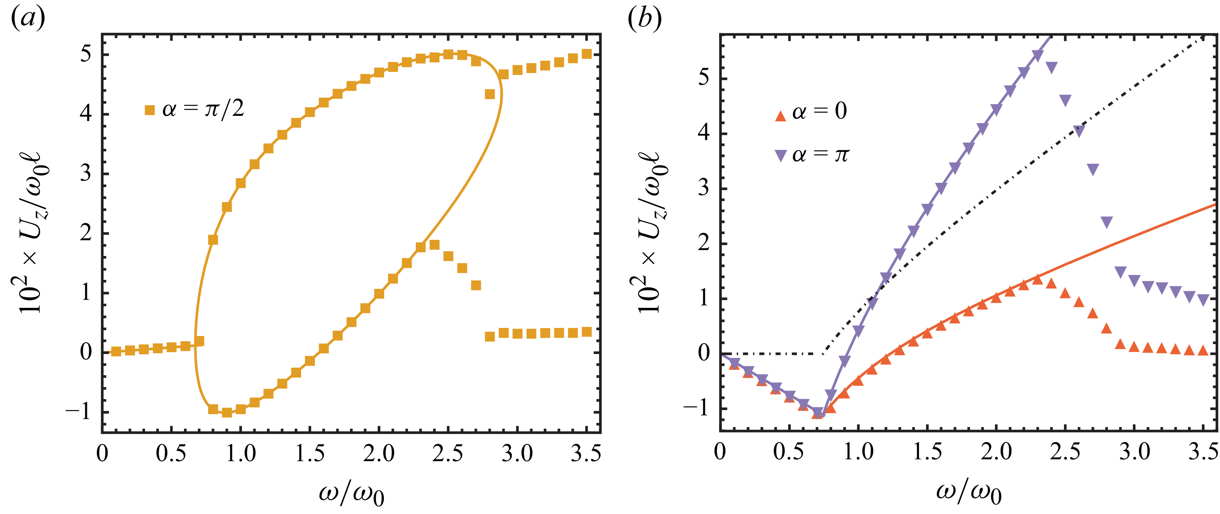


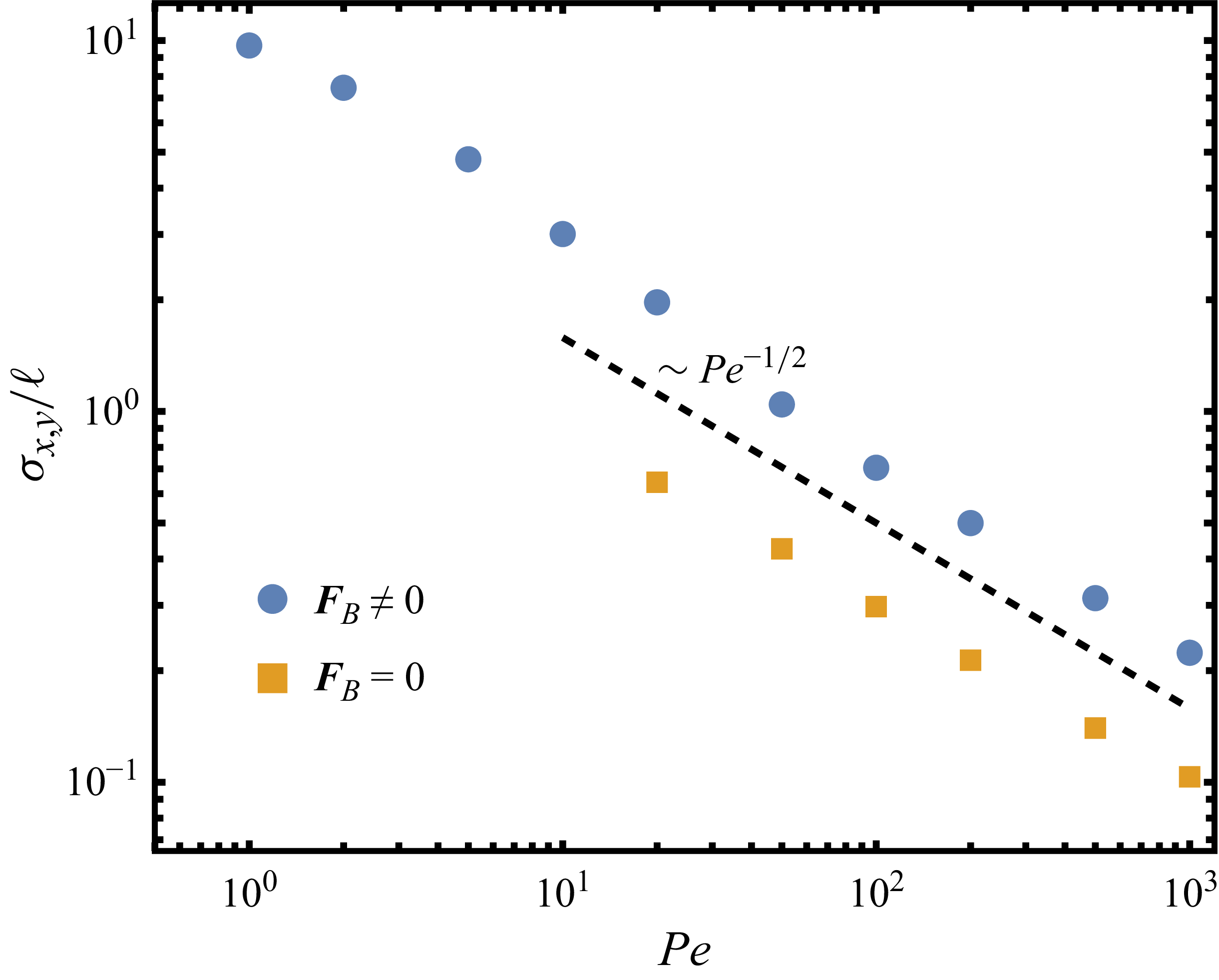


 Open access