


1 Introduction
Robust design processes are important to sustained business success. Engineering design processes involve the effort of many people performing multiple and varied activities in order to obtain a common goal such as the development of a product (Eppinger & Ulrich Reference Eppinger and Ulrich2015). Design processes are usually modelled as activity/task networks and widely recognised as complex systems, where the way elements are interconnected changes the behaviour of the system (Eppinger & Browning Reference Eppinger and Browning2012). People implement the design process performing multiple activities. Despite such interactions between people and activities, most of the knowledge about the two systems comes from studies which consider them as separated systems (Eppinger & Browning Reference Eppinger and Browning2012).
The way elements are interconnected also impacts the system’s robustness. Here, differently from robust design and robustness related to technical systems (Göhler, Eifler & Howard Reference Göhler, Eifler and Howard2016), we are focused on the robustness of design processes as systems of people working on activities. As in previous work, we define robustness of a system as the ability of the system to maintain its functions or performance even after errors or failures of some of its components (Albert, Jeong & Barabási Reference Albert, Jeong and Barabási2000; Braha Reference Braha2016). Robustness is related to the dependencies of the system. When we represent a system as a network, these dependencies can be represented as the network structure, its topology. Let us use a Local Area Network (LAN) as an example where nodes are routers or, generally, devices that send packets through the network and edges are physical links or other suitable channels in which packets can flow from one node to another. If the topology of the LAN is a star where all the peripheral routers are connected to a central node then a malfunction in the central node will prevent any possible communication in the network. If the topology is the complete graph where each node is connected to every other node then a failure will only affect the failing node and any other communication in the network is still possible.
Here, we investigate topology and robustness of a design process by considering people and activities together. Likewise, when considering a design process where people work on activities, the robustness of the design process is related to the dependencies between these two entities. If an activity fails then all the people working on that activity will be affected in that the output of the activity will be unavailable to all of them. Furthermore, the output of the failed activity will be unavailable to all the other dependent activities. Similarly, if a person working on more than one activity is unable to work, information may not flow from one activity to another. These glitches may result in delays or, in more severe cases, even in the failure of the whole design process. Thus, we ask: in what way is a design process robust? How robust is the design process to random failures? How robust is the design process to targeted failures or cascades? How do people and activities influence the robustness of a design process?
Previous work on robustness of the design process focused on the analysis of interconnections between activities and – by studying how errors propagate – showed that activity networks are error tolerant but vulnerable to perturbations targeted at specific central tasks (Braha & Bar-Yam Reference Braha and Bar-Yam2007). Concurrently, the same central activities, if improved and therefore less error prone, help the process converge faster (Braha & Bar-Yam Reference Braha and Bar-Yam2007). Activity networks provide a convenient representation that makes it possible to effectively plan and manage the design process. However, the design process is implemented by people who work on the activities and make the flow of information possible. Therefore, the study of interactions between people and activities can provide important information about the implementation of a process.
In projects where each person works on only one activity, interaction between people and activities is straightforward and its study would not provide much information. However, many real-world projects are complex and require people working on more than one activity, while, at the same time, collaborating with other people on common activities. Such interactions give rise to an interesting network topology describing the interplay between people and activities: a bipartite network.
Here, using data about the design of a biomass power plant (see also Materials and Methods), we model the design process as a bipartite network of people and activities to study the role of these two entities: how their interconnections influence the system and whether one set of nodes is more central to process robustness. In this paper, we analyse the robustness of the design process with respect to activities and people making the following three main contributions.
First, we derive insights from our data. We consider the problem of resource availability by removing people from the network and activity failures by removing activities from the network. We show that our design process is resistant to problems in resource availability and activity failures when they happen at random. However, the process is fragile if problems target central people or activities. Specifically, we show that the design process is more vulnerable to removal of highly connected people than it is to removal of activities with many participants. Failures with respect to central activities increase the local vulnerability, while failures with respect to central people increase the global vulnerability.
Second, we generalise the previous findings using simulations to show that the behaviour described above is dictated by the degree distributions of people and activities. Specifically, we find the same behaviour as described above in a degree conserving null model system which maintains degree distributions, but randomises all other connections. In a homogeneous null model system where connections are completely random, as in not maintaining the degree distributions, the observed behaviour changes.
Finally, we link topology and dynamics. We consider ‘cascading failures’ (Crucitti, Latora & Marchiori Reference Crucitti, Latora and Marchiori2004; Braha & Bar-Yam Reference Braha and Bar-Yam2007) by simulating a dynamical process of error propagation, linking the considerations with resource availability and activity failures to systemic risk. By studying this scenario in (a) the original network, (b) an improved version of it, and (c) a homogeneous null model network where the degree distributions are equalised, we show that a more optimal assignment of people to activities, which addresses the problem of resource availability, also produces a network which is more resistant to cascading failures.
2 Background and related work
With the goal of evaluating design process robustness, we draw upon the intersection between engineering design and network science to progress from unidimensional analyses to multidimensional analyses. To this end, as we have data that directly connect people to the activities they perform, we build our approach on bipartite networks, which are a special class of networks to enable the joint analysis of two kinds of nodes.
2.1 Intersecting engineering design and network science
The design process involves many people working and collaborating on multiple different activities that require a varied set of skills (Bucciarelli Reference Bucciarelli1994; Eppinger & Ulrich Reference Eppinger and Ulrich2015). Research on the design process recognises the importance of interconnections between the elements of study, including people, activities, components, and the context within which designing takes place, thus the need of methods to deal with connections and complexity of the examined systems. With the focus of this paper being on the bipartite network of people and activities, we mark the discussion on applications of network science to networks of components in a product out of scope and refer to works, e.g. by Sharman & Yassine (Reference Sharman and Yassine2004) or Eppinger & Browning (Reference Eppinger and Browning2012).
Graph theoretic approaches are convenient tools to analyse systems of interconnected parts (Newman Reference Newman2003; Easley & Kleinberg Reference Easley and Kleinberg2010; Newman Reference Newman2010; Albert & Barabási Reference Albert and Barabási2002). They provide a minimal general description framework based on a representation using nodes and edges only, have visual power using both matrix and graph forms and are built on elegant mathematical foundations (Bondy Reference Bondy1976). Because of its flexibility and ability to model complex systems, network science has become increasingly popular in many scientific fields (Easley & Kleinberg Reference Easley and Kleinberg2010; Newman Reference Newman2010). To provide some examples of the broad applications of networks outside the engineering domain, we mention molecular biology (Milo et al. Reference Milo, Shen-Orr, Itzkovitz, Kashtan, Chklovskii and Alon2002; Guimera & Amaral Reference Guimera and Amaral2005; Thiery & Sleeman Reference Thiery and Sleeman2006), brain research (Bullmore & Sporns Reference Bullmore and Sporns2009), information retrieval (Brin & Page Reference Brin and Page1998; Kleinberg Reference Kleinberg1999), and recipe recommendation (Teng, Lin & Adamic Reference Teng, Lin and Adamic2012).
To date, application of network science to the study of engineering design processes has mainly taken two perspectives: the organisational structure as network of people and the process structure as network of activities. In the design literature, networks are commonly visualised as matrices using what was termed Design Structure Matrices (DSMs) (Steward Reference Steward1981).
Organisational networks have been studied in the fields of social science and management (Granovetter Reference Granovetter1973; Krackhardt & Hanson Reference Krackhardt and Hanson1993; Wasserman & Faust Reference Wasserman and Faust1994; Burt Reference Burt2009; Štorga, Mostashari & Stanković Reference Štorga, Mostashari and Stanković2013) to show how the informal network, as opposed to formal organisational hierarchy, determines roles, work, coordination, and to show how people can use structural holes to act as social brokers. Consequently, organisational networks have been adopted to redesign the organisational structure to enhance communication, plan the arrangement of new offices to better support interpersonal communication, analyse stakeholders’ influence, and so forth (Allen Reference Allen1977; Eppinger & Browning Reference Eppinger and Browning2012).
Activity networks have been studied, for example, to model the process (Browning & Ramasesh Reference Browning and Ramasesh2007; Braha Reference Braha2016), to reduce iterations (Yassine Reference Yassine2007), to sequence activities (Meier, Yassine & Browning Reference Meier, Yassine and Browning2007), to modularise (partition) the process (Seol et al. Reference Seol, Kim, Lee and Park2007), to relate effects of process architecture to project cost (Eppinger & Browning Reference Eppinger and Browning2012). Braha & Bar-Yam (Reference Braha and Bar-Yam2004a ,Reference Braha and Bar-Yam b , Reference Braha and Bar-Yam2007) found that activity networks from large-scale projects exhibit the small-world property (Watts & Strogatz Reference Watts and Strogatz1998) and right skewed degree distributions. The small-world property implies that information, changes, and errors can propagate fast in these networks. Right skewed degree distributions imply that there are many activities with a low number of connections and few activities with a high number of connections. Activities with high connectivity dominate dynamical processes occurring on the network. In this regard, activity networks exhibit the properties that characterise complex networks (Albert & Barabási Reference Albert and Barabási2002; Newman Reference Newman2003); these properties are common to many other natural and man-made networks (Easley & Kleinberg Reference Easley and Kleinberg2010; Newman Reference Newman2010). Braha & Bar-Yam (Reference Braha and Bar-Yam2007) and Braha (Reference Braha2016) also found that activity networks show negative or no degree assortativity (see Materials and Methods), interpreting this feature as a way to suppress the propagation of errors and changes in the network.
Taking the growing complexity of modern engineering projects into consideration, companies experience the need to jointly plan, manage, and analyse more than one domain. Thus, approaches based on Domain Mapping Matrices (DMMs) (Danilovic & Browning Reference Danilovic and Browning2007), Multiple Domain Matrices (MDMs) (Lindemann, Maurer & Braun Reference Lindemann, Maurer and Braun2008; Bartolomei et al. Reference Bartolomei, Hastings, de Neufville and Rhodes2012; Eppinger & Browning Reference Eppinger and Browning2012), and multilayer networks (Kivelä et al. Reference Kivelä, Arenas, Barthelemy, Gleeson, Moreno and Porter2014) were developed.
These approaches have been used for multiple purposes, including to compose teams for collaboration between design and simulation departments (Kreimeyer et al. Reference Kreimeyer, Deubzer, Danilovic, Fuchs, Herfeld and Lindemann2007), to understand customer preferences by simultaneously considering customers, products and their relations (Wang et al. Reference Wang, Chen, Huang, Contractor and Fu2016), and to explore security threats (Eppinger & Browning Reference Eppinger and Browning2012).
2.2 Bipartite networks
Bipartite networks are a special class of networks consisting of two types of nodes and connections are allowed only between nodes of different types; that is, the two node sets are disjoint. Many real-world networks present this bipartition: human disease networks (Goh et al. Reference Goh, Cusick, Valle, Childs, Vidal and Barabási2007), co-author networks (Jesus, Schwartz & Lehmann Reference Jesus, Schwartz and Lehmann2009), social networks (Lambiotte & Ausloos Reference Lambiotte and Ausloos2005; Borgatti & Halgin Reference Borgatti and Halgin2014), company board networks (Robins & Alexander Reference Robins and Alexander2004), engineering networks (Eppinger & Browning Reference Eppinger and Browning2012) and many others (Latapy, Magnien & Vecchio Reference Latapy, Magnien and Vecchio2008; Lehmann, Schwartz & Hansen Reference Lehmann, Schwartz and Hansen2008).
Beyond the analysis of the nodes composing the network, the applications of bipartite networks are varied. We mention, as examples, studying the spread of sexually transmissible diseases in heterogeneous populations (Gómez-Gardeñes et al. Reference Gómez-Gardeñes, Latora, Moreno and Profumo2008), analysing collective listening habits (Lambiotte & Ausloos Reference Lambiotte and Ausloos2005), providing personal recommendations (Zhou et al. Reference Zhou, Ren, Medo and Zhang2007), and investigating the importance of human genes that encode hub proteins (Goh et al. Reference Goh, Cusick, Valle, Childs, Vidal and Barabási2007). In the domain of engineering design a bipartite representation has been used, for example, to describe connections between tasks and the attributes they have in common in order to partition tasks among a number of development teams (Braha Reference Braha2002) and to manage product development projects (Danilovic & Browning Reference Danilovic and Browning2007).
The importance of bipartite networks has also been demonstrated from a theoretical standpoint. Guillaume & Latapy (Reference Guillaume and Latapy2004, Reference Guillaume and Latapy2006) have shown that all networks can be viewed as bipartite structures and that the basic properties of networks such as degree distribution, clustering coefficient, and average distance can be viewed as consequences of this underlying bipartite structure.
Bipartite networks have been studied in multiple ways. Arguably, the most common method to deal with bipartite networks is the use of a projection: the structure of the bipartite network is projected to one node set. Subsequently, usual analysis techniques are employed on the resulting network (Albert & Barabási Reference Albert and Barabási2002; Newman Reference Newman2003). A projection consists of connecting two nodes from one node set and uses the number of common nodes from the other node set they are connected to as weight. This method suffers from information loss which can manifest itself in different ways: (1) the projection may create non-significant links and over-represent the density of the network; (2) the projection is one-way only, as many different bipartite configurations can result in the same projected configuration, as, for example, shown in Figure 1.
Two different bipartite configurations produce the same configuration after the application of a bipartite network projection. The configuration on the left is a star (non-cyclic configuration) which results in a triangle (cycle) after the projection. The configuration on the right is a cycle between six nodes and also results in a triangle after the projection. However, there is no possibility to distinguish between the two. In both cases the information about the other node set is lost. Thus, a direct analysis of the bipartite network, without relying on projections, is preferable.

A central problem, however, is that the mathematical tools for analysing bipartite networks are not as developed as the tools for analysing standard (unipartite) networks. Two strategies have typically been used to in the analysis of bipartite networks. The first strategy consists of using a double projection approach resulting in two different networks (one per node set) which can then be analysed separately and compared (Breiger Reference Breiger1974; Goh et al. Reference Goh, Cusick, Valle, Childs, Vidal and Barabási2007; Everett & Borgatti Reference Everett and Borgatti2013). The second strategy, instead, specifically targets the creation of non-significant links and the over-representation of the network density and clustering coefficient (Tumminello et al. Reference Tumminello, Aste, Di Matteo and Mantegna2005; Zweig & Kaufmann Reference Zweig and Kaufmann2011; Neal Reference Neal2014). The idea, common to these approaches, is to retain only statistically significant links in the projected network.
While these countermeasures help to mitigate the problem, the projection of a bipartite network to one node set, even the double projection, will lose the information about the interplay between the two node sets, i.e. the links connecting nodes from two different node sets. As such, a different approach is given by the direct analysis of the bipartite network. This may require to re-define approaches originally developed for unipartite networks for applicability to bipartite networks, or to define new measures. In this regard, Faust (Reference Faust1997), Borgatti & Halgin (Reference Borgatti and Halgin2014), and Bonacich (Reference Bonacich1991) defined centrality measures for bipartite networks, generalising previous definitions of centrality measures of unipartite networks. Borgatti & Everett (Reference Borgatti and Everett1997) focused on node centrality and network centralisation measures and on subgroups in affiliation networks.
Further, the clustering coefficient measure has been re-defined in multiple ways: in terms of cycles of a length of four (Robins & Alexander Reference Robins and Alexander2004; Lind, González & Herrmann Reference Lind, González and Herrmann2005) as a measure of cliquishness of the network, in terms of degree of neighbourhood overlapping (Latapy et al. Reference Latapy, Magnien and Vecchio2008) to capture the likelihood that if two nodes are connected they also share some common neighbours, and in terms of cycles of a length of six (Opsahl Reference Opsahl2013) to capture the triadic closure between three nodes.
The problem of finding subgroups has been tackled for example in Lehmann et al. (Reference Lehmann, Schwartz and Hansen2008), where the authors defined a clustering algorithm to find modules in a bipartite network based on adjacent bi-cliques. They applied their algorithm to a scientific collaboration network of authors and papers, showing how the direct clustering on the bipartite network can provide more information than the clustering on a projection. Finally, bipartite networks can also be analysed with Galois lattices (Bonacich Reference Bonacich1978; Freeman & White Reference Freeman and White1993) and with any matrix approach for rectangular matrices such as singular value decomposition (SVD).
2.3 Network robustness
As systems can be modelled with networks, their robustness can be investigated using their network topology. Here, robustness of a system is the system’s ability to react to failures of its components; thus, a system is robust if it can maintain its functions even if some of its components fail or stop interacting (Albert et al. Reference Albert, Jeong and Barabási2000). Albert et al. (Reference Albert, Jeong and Barabási2000) studied the robustness of two classes of networks: homogeneous random networks that have Poisson degree distribution (the degree of a node is its number of connections) and scale-free networks (Barabási & Albert Reference Barabási and Albert1999) that have power-law degree distribution. The reason to compare random networks against scale-free networks was that many real-world networks are not random and their degree distributions are broad, resembling power laws. This means that in real-world networks there are very few nodes having a high number of connections and a large number of nodes with very few connections. Albert et al. (Reference Albert, Jeong and Barabási2000) simulated random failures by random removal of nodes and targeted attacks (by removing nodes according to their degree, from the highest to the lowest). They observed that while random networks are resistant to both random failures and targeted attacks, scale-free networks are resistant to random failures but highly vulnerable to targeted attacks.
Similar results have been found in other classes of networks and relations between topology and robustness have been further investigated (Callaway et al. Reference Callaway, Newman, Strogatz and Watts2000; Cohen, ben Avraham & Havlin Reference Cohen, ben Avraham and Havlin2002; Schwartz et al. Reference Schwartz, Cohen, ben Avraham, Barabási and Havlin2002; Dekker & Colbert Reference Dekker and Colbert2004). The impact of removing nodes according to other centrality measures rather than the degree has also been considered (Iyer et al. Reference Iyer, Killingback, Sundaram and Wang2013). Furthermore, modular networks have been found to be vulnerable also to random failures as these failures can disrupt the cohesiveness of modules and thereby make the network vulnerable (Bagrow, Lehmann & Ahn Reference Bagrow, Lehmann and Ahn2015).
A complementary way of defining robustness, as opposed to removing nodes from the network, is by simulating a dynamical process which allows us to evaluate how nodes or links degrade over time. For example, Crucitti et al. (Reference Crucitti, Latora and Marchiori2004) proposed a dynamic model for cascading failures. They model the degradation of connections subsequent to a node failure, measuring the downstream network efficiency. The idea is that each node of the network can support a certain load, and if the load is exceeded, the node fails and its load is redistributed to every other node in the network. They used this model to demonstrate how even a single failure can trigger cascades that affect the whole network efficiency.
Other tools to define robustness or resilience in a dynamic fashion are offered by the study of epidemics on networks (Pastor-Satorras & Vespignani Reference Pastor-Satorras and Vespignani2001). Pastor-Satorras & Vespignani (Reference Pastor-Satorras and Vespignani2001) showed how scale-free networks do not have an intrinsic epidemic threshold, meaning that infections can propagate on scale-free networks regardless of the spreading rate. At the same time they showed how strategies of immunisation targeted at nodes with a high number of connections can drastically lower the vulnerability of the network Pastor-Satorras & Vespignani (Reference Pastor-Satorras and Vespignani2002).
In the domain of engineering design, using activity networks to represent product development processes, Braha & Bar-Yam (Reference Braha and Bar-Yam2007) modelled the dynamics of error propagation studying the mean convergence time of design processes. They found that product development networks are very robust if errors happen at random, yet very fragile if errors happen at highly connected activities, increasing the convergence time. Braha & Bar-Yam (Reference Braha and Bar-Yam2007) also found that improving highly connected activities, making them less error prone, decreases the convergence time of the entire process.
To respond to the vulnerability of networks by increasing their robustness, a number of approaches to network rewiring have been proposed (Beygelzimer et al. Reference Beygelzimer, Grinstein, Linsker and Rish2005; Tanizawa et al. Reference Tanizawa, Paul, Cohen, Havlin and Stanley2005; Louzada et al. Reference Louzada, Daolio, Herrmann and Tomassini2013).
3 Materials and methods
3.1 Data
To evaluate process robustness and the interplay between people and activities, in this paper we analyse data from a Danish organisation involved in the design of power plants. Our data refer to the design stage of a large project ( $\unicode[STIX]{x00A3}$
160,000,000
$\unicode[STIX]{x00A3}$
160,000,000 $+$
) of a renewable energy power plant for electrical energy generation (Parraguez, Eppinger & Maier Reference Parraguez, Eppinger and Maier2015). From the company, the design stage involved
$+$
) of a renewable energy power plant for electrical energy generation (Parraguez, Eppinger & Maier Reference Parraguez, Eppinger and Maier2015). From the company, the design stage involved $111$
individuals distributed across
$111$
individuals distributed across $14$
functional units. The workload was organised in
$14$
functional units. The workload was organised in $148$
activities partitioned in
$148$
activities partitioned in $13$
activity groups. We use the activity granularity originally defined by the company to retain the most detailed description of the system. The bipartite network which maps people to activities was obtained from the activity and document logs used by the company to register the tasks on which each person worked. Using the terminology of design structure matrices, the bipartite network is also known as Domain Mapping Matrix (DMM) (Danilovic & Browning Reference Danilovic and Browning2007). The resulting network has 259 nodes (111 people
$13$
activity groups. We use the activity granularity originally defined by the company to retain the most detailed description of the system. The bipartite network which maps people to activities was obtained from the activity and document logs used by the company to register the tasks on which each person worked. Using the terminology of design structure matrices, the bipartite network is also known as Domain Mapping Matrix (DMM) (Danilovic & Browning Reference Danilovic and Browning2007). The resulting network has 259 nodes (111 people $+$
148 activities) and 926 links person–activity, meaning that the average number of activities each person worked on is
$+$
148 activities) and 926 links person–activity, meaning that the average number of activities each person worked on is ${\sim}8.34$
.
${\sim}8.34$
.
Descriptive statistics for the bipartite network

Table 1 reports some descriptive statistics for our network. The network is sparse ( $\unicode[STIX]{x1D6FF}_{G}=0.056$
) and shows the small-world property (Watts & Strogatz Reference Watts and Strogatz1998). The average shortest path length of the network (
$\unicode[STIX]{x1D6FF}_{G}=0.056$
) and shows the small-world property (Watts & Strogatz Reference Watts and Strogatz1998). The average shortest path length of the network ( $l_{G}$
) is comparable to the average shortest path length that we would expect in a random bipartite graph with the same number of nodes and edges (
$l_{G}$
) is comparable to the average shortest path length that we would expect in a random bipartite graph with the same number of nodes and edges ( $l_{Rand}$
), while the clustering coefficient (
$l_{Rand}$
), while the clustering coefficient ( $C_{G}$
) is much higher than what we would expect in a random graph (
$C_{G}$
) is much higher than what we would expect in a random graph ( $C_{Rand}$
). Other design process networks have been found to be small world, too (Braha & Bar-Yam Reference Braha and Bar-Yam2004a
,Reference Braha and Bar-Yam
b
).
$C_{Rand}$
). Other design process networks have been found to be small world, too (Braha & Bar-Yam Reference Braha and Bar-Yam2004a
,Reference Braha and Bar-Yam
b
).
3.2 Bipartite networks and measures
A bipartite network is a triple $G(V_{1},V_{2},E)$
, where
$G(V_{1},V_{2},E)$
, where $V_{1}$
and
$V_{1}$
and $V_{2}$
are the two node sets, and
$V_{2}$
are the two node sets, and $E$
is the set of edges. In a bipartite network, edges are only allowed between the two node sets. A bipartite network can be represented by its bi-adjacency matrix
$E$
is the set of edges. In a bipartite network, edges are only allowed between the two node sets. A bipartite network can be represented by its bi-adjacency matrix $\mathbf{B}$
in which
$\mathbf{B}$
in which $b_{i,j}=1$
if and only if
$b_{i,j}=1$
if and only if $(v_{i},v_{j})\in E$
.
$(v_{i},v_{j})\in E$
.
3.2.1 Global measures
Density. The density $\unicode[STIX]{x1D6FF}_{G}$
of a given graph
$\unicode[STIX]{x1D6FF}_{G}$
of a given graph $G$
is defined as the ratio of the actual number of edges in
$G$
is defined as the ratio of the actual number of edges in $E$
to the number of all the possible edges; that is
$E$
to the number of all the possible edges; that is
 $$\begin{eqnarray}\unicode[STIX]{x1D6FF}_{G}=\frac{|E|}{|V_{1}|\times |V_{2}|}.\end{eqnarray}$$
Average degree. The average degree $\langle k\rangle$
is defined as the sum of the edges incident on each node over the number of nodes. With
$\langle k\rangle$
is defined as the sum of the edges incident on each node over the number of nodes. With $k_{i}$
being the degree of node
$k_{i}$
being the degree of node $i$
, the average degree is defined as
$i$
, the average degree is defined as
 $$\begin{eqnarray}\langle k\rangle =\frac{\mathop{\sum }_{i}k_{i}}{|V_{1}|+|V_{2}|}.\end{eqnarray}$$
Average shortest path length. Let $d(i,j)$
, where
$d(i,j)$
, where $i,j\in V$
denote the shortest distance between nodes
$i,j\in V$
denote the shortest distance between nodes $i$
and
$i$
and $j$
, the average shortest path length
$j$
, the average shortest path length $l_{G}$
is defined as
$l_{G}$
is defined as
 $$\begin{eqnarray}l_{G}=\frac{1}{2\times |V_{1}|\times |V_{2}|}\mathop{\sum }_{i\neq j}d(i,j).\end{eqnarray}$$
Diameter. The diameter of a graph is the maximum shortest distance between two nodes in the graph.
 $$\begin{eqnarray}D_{G}=\max _{i,j}d(i,j).\end{eqnarray}$$
Clustering coefficient. We use the definition of bipartite clustering coefficient provided by Robins & Alexander (Reference Robins and Alexander2004). This definition captures the cliquishness of the network and it is defined by the smallest possible cycle and smallest complete graph in two-mode networks: the square, a closed path of length four. The clustering coefficient is defined as the ratio of the number of squares to the number of paths of length three (also called quadruplets as they involve four nodes). Let $C_{4}$
denote the number of squares and
$C_{4}$
denote the number of squares and $L_{3}$
the number of quadruplets in
$L_{3}$
the number of quadruplets in $G$
, the clustering coefficient
$G$
, the clustering coefficient $C_{G}$
is
$C_{G}$
is
 $$\begin{eqnarray}C_{G}=\frac{C_{4}}{L_{3}}.\end{eqnarray}$$
It may be worth noting the similarity between $C_{G}$
and the clustering coefficient for one-mode networks defined as the ratio of the number of triangles to the number of triplets (Wasserman & Faust Reference Wasserman and Faust1994).
$C_{G}$
and the clustering coefficient for one-mode networks defined as the ratio of the number of triangles to the number of triplets (Wasserman & Faust Reference Wasserman and Faust1994).
The clustering coefficient can also be computed at a node level with the same formula by centring the calculations on the node under analysis.
Degree assortativity coefficient. The degree assortativity coefficient is defined as the Pearson correlation coefficient of the degrees at either ends of an edge (Newman Reference Newman2002) and lies in the range $-1\leqslant r\leqslant 1$
. It expresses the extent to which nodes with similar degrees are connected together in the network.
$-1\leqslant r\leqslant 1$
. It expresses the extent to which nodes with similar degrees are connected together in the network.
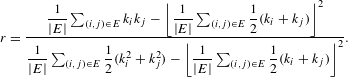 $$\begin{eqnarray}r=\frac{{\displaystyle \frac{1}{|E|}}\mathop{\sum }_{(i,j)\in E}k_{i}k_{j}-\left\lfloor {\displaystyle \frac{1}{|E|}}\mathop{\sum }_{(i,j)\in E}{\displaystyle \frac{1}{2}}(k_{i}+k_{j})\right\rfloor ^{2}}{{\displaystyle \frac{1}{|E|}}\mathop{\sum }_{(i,j)\in E}{\displaystyle \frac{1}{2}}(k_{i}^{2}+k_{j}^{2})-\left\lfloor {\displaystyle \frac{1}{|E|}}\mathop{\sum }_{(i,j)\in E}{\displaystyle \frac{1}{2}}(k_{i}+k_{j})\right\rfloor ^{2}}.\end{eqnarray}$$
In a bipartite network, this assortativity coefficient expresses the extent by which nodes in the two node sets with similar degrees are connected together. Positive values of $r$
indicate that nodes with high (low) degree in
$r$
indicate that nodes with high (low) degree in $V_{1}$
are connected to nodes with high (low) degree in
$V_{1}$
are connected to nodes with high (low) degree in $V_{2}$
and vice versa. In this case the network is said to be assortative. Negative values of
$V_{2}$
and vice versa. In this case the network is said to be assortative. Negative values of $r$
indicate that nodes with high (low) degree in
$r$
indicate that nodes with high (low) degree in $V_{1}$
are connected to nodes with low (high) degree in
$V_{1}$
are connected to nodes with low (high) degree in $V_{2}$
and vice versa. In this case the network is said to be disassortative.
$V_{2}$
and vice versa. In this case the network is said to be disassortative.
3.2.2 Local measures and centrality
Degree centrality. The degree captures the extent to which a node is important in the network by counting its direct connections: the higher the number of connections the more important a node. Despite its simplicity, the degree can be an effective measure of importance and it has been useful to show crucial differences between random and complex networks (Albert & Barabási Reference Albert and Barabási2002), in that complex networks show heavy-tailed degree distributions as opposed to random networks that show Poisson-like degree distributions.
Given that in two-mode networks the two sets $V_{1}$
and
$V_{1}$
and $V_{2}$
can have different sizes, it is a good idea to normalise the degree by the maximum number of possible connections for the two different sets (Borgatti & Halgin Reference Borgatti and Halgin2014). Let
$V_{2}$
can have different sizes, it is a good idea to normalise the degree by the maximum number of possible connections for the two different sets (Borgatti & Halgin Reference Borgatti and Halgin2014). Let $k_{i}$
be the degree of the node
$k_{i}$
be the degree of the node $i$
, the normalised degree centrality
$i$
, the normalised degree centrality $DC(i)$
is:
$DC(i)$
is:
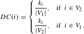 $$\begin{eqnarray}DC(i)=\left\{\begin{array}{@{}ll@{}}{\displaystyle \frac{k_{i}}{|V_{1}|}},\quad & \text{if }~i\in V_{2}\\ {\displaystyle \frac{k_{i}}{|V_{2}|}},\quad & \text{if }~i\in V_{1}.\end{array}\right.\end{eqnarray}$$
Betweenness centrality. The betweenness centrality (Freeman Reference Freeman1977) captures the ability of a node to bridge separated parts of the network, thus how much a node has a broker-like position. The betweenness centrality measure of a node $i$
is, thus, defined as the sum of the fraction of all-pairs shortest paths that pass through
$i$
is, thus, defined as the sum of the fraction of all-pairs shortest paths that pass through $i$
. Let
$i$
. Let $\unicode[STIX]{x1D70E}_{jk}$
be the number of shortest paths from node
$\unicode[STIX]{x1D70E}_{jk}$
be the number of shortest paths from node $j$
to node
$j$
to node $k$
and let
$k$
and let $\unicode[STIX]{x1D70E}_{jk}(i)$
be the number of shortest paths from
$\unicode[STIX]{x1D70E}_{jk}(i)$
be the number of shortest paths from $j$
to
$j$
to $k$
passing through
$k$
passing through $i$
, the betweenness centrality
$i$
, the betweenness centrality $BC(i)$
is:
$BC(i)$
is:
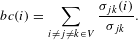 $$\begin{eqnarray}bc(i)=\mathop{\sum }_{i\neq j\neq k\in V}\frac{\unicode[STIX]{x1D70E}_{jk}(i)}{\unicode[STIX]{x1D70E}_{jk}}.\end{eqnarray}$$
Values of betweenness can be normalised dividing them for the maximum possible value which for bipartite graphs depends on the relative size of the two node sets (Borgatti & Halgin Reference Borgatti and Halgin2014).
 $$\begin{eqnarray}\begin{array}{@{}rcl@{}}b_{V_{1}max}\ & =\ & \frac{1}{2}[|V_{2}|^{2}(s+1)^{2}+|V_{2}|(s+1)(2t-s-1)-t(2s-t+3)]\\ \ & \ & s=(|V_{1}|-1)\div |V_{2}|,\quad t=(|V_{1}|-1)\hspace{0.6em}{\rm mod}\hspace{0.2em}|V_{2}|\\ b_{V_{2}max}\ & =\ & \frac{1}{2}[|V_{1}|^{2}(p+1)^{2}+|V_{1}|(p+1)(2r-p-1)-r(2p-r+3)]\\ \ & \ & p=(|V_{2}|-1)\div |V_{1}|,\quad r=(|V_{2}|-1)\hspace{0.6em}{\rm mod}\hspace{0.2em}|V_{1}|.\end{array}\end{eqnarray}$$
Thus, we can now define the normalised betweenness centrality $BC(i)$
dividing the values obtained from Eq. (8) by the appropriate maximum in Eq. (9).
$BC(i)$
dividing the values obtained from Eq. (8) by the appropriate maximum in Eq. (9).
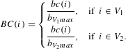 $$\begin{eqnarray}BC(i)=\left\{\begin{array}{@{}ll@{}}{\displaystyle \frac{bc(i)}{b_{V_{1}max}}},\quad & \text{if }~i\in V_{1}\\ {\displaystyle \frac{bc(i)}{b_{V_{2}max}}},\quad & \text{if }~i\in V_{2}.\end{array}\right.\end{eqnarray}$$
Closeness centrality. The closeness centrality (Bavelas Reference Bavelas1948) of a node was defined as the inverse of its distance to all the other nodes. By capturing how much a node is close to all the other nodes in the network, closeness centrality can be interpreted, complimentary to betweenness, as a measure of independence to brokerage. Indeed, in some experiments performed to study collaboration in groups of people, it was shown that people perceived as leaders where those ones with high closeness values (Bavelas Reference Bavelas1948, Reference Bavelas1950). Let $d(i,j)$
, where
$d(i,j)$
, where $i,j\in V$
denote the shortest distance between nodes
$i,j\in V$
denote the shortest distance between nodes $i$
and
$i$
and $j$
, the closeness centrality for a given node
$j$
, the closeness centrality for a given node $i$
is:
$i$
is:
 $$\begin{eqnarray}cc(i)=\frac{1}{\mathop{\sum }_{j\neq i\in V}d(i,j)}.\end{eqnarray}$$
Values of closeness can be normalised dividing them for the maximum possible value of closeness in a bipartite graph relative to the node’s set (Borgatti & Halgin Reference Borgatti and Halgin2014). Thus, the normalised closeness centrality $CC(i)$
is:
$CC(i)$
is:
 $$\begin{eqnarray}CC(i)=\left\{\begin{array}{@{}ll@{}}{\displaystyle \frac{|V_{2}|+2(|V_{1}|-1)}{cc(i)}},\quad & \text{if }~i\in V_{1}\\ {\displaystyle \frac{|V_{1}|+2(|V_{2}|-1)}{cc(i)}},\quad & \text{if }~i\in V_{2}.\end{array}\right.\end{eqnarray}$$
Eigenvector centrality. Measures analysed so far have a common property: they measure the importance of a node from its properties. In the case of the degree, edges are even considered in the same way, i.e. degree centrality cannot assign different scores to nodes that have the same number of connections, but connections are not necessarily equal and some nodes can have better connections than others. Eigenvector centrality (Bonacich Reference Bonacich1972) acknowledges that connections are not necessarily equal and a node with fewer connections can be more important than a node with many more connections. Differently from betweenness and closeness centrality, eigenvector centrality defines the importance of a node in function of the importance of the nodes to which it is connected: a node is important if it is connected to important nodes. The eigenvector centrality of a node $i$
is:
$i$
is:
 $$\begin{eqnarray}EC(i)=\frac{1}{\unicode[STIX]{x1D706}}\mathop{\sum }_{j\in \unicode[STIX]{x1D6E4}(i)}EC(j)\end{eqnarray}$$
where $\unicode[STIX]{x1D706}$
is a constant and
$\unicode[STIX]{x1D706}$
is a constant and $\unicode[STIX]{x1D6E4}(i)$
is the neighbourhood of node
$\unicode[STIX]{x1D6E4}(i)$
is the neighbourhood of node $i$
, i.e. the set of nodes connected to
$i$
, i.e. the set of nodes connected to $i$
. Let us denote as
$i$
. Let us denote as $\mathbf{x}$
a
$\mathbf{x}$
a $|V|$
-dimensional column vector such that
$|V|$
-dimensional column vector such that $\mathbf{x}[i]=EC(i)$
, Eq. (13) can be rewritten as the eigenvector equation:
$\mathbf{x}[i]=EC(i)$
, Eq. (13) can be rewritten as the eigenvector equation:
 $$\begin{eqnarray}\mathbf{Ax}=\unicode[STIX]{x1D706}\mathbf{x}.\end{eqnarray}$$
If we impose that centrality indices must be non-negative, the Perron–Frobenius theorem ensures that Eq. (14) has a unique solution, which is the eigenvector corresponding to the largest eigenvalue $\unicode[STIX]{x1D706}$
of
$\unicode[STIX]{x1D706}$
of $\mathbf{A}$
. Eq. (14) is directly applicable to bipartite graphs (Bonacich Reference Bonacich1991) and is identical to the singular value decomposition of the bi-adjacency matrix
$\mathbf{A}$
. Eq. (14) is directly applicable to bipartite graphs (Bonacich Reference Bonacich1991) and is identical to the singular value decomposition of the bi-adjacency matrix $\text{}\text{B}$
(Borgatti & Halgin Reference Borgatti and Halgin2014), thus yielding the measures of hubs and authorities proposed by Kleinberg (Reference Kleinberg1999).
$\text{}\text{B}$
(Borgatti & Halgin Reference Borgatti and Halgin2014), thus yielding the measures of hubs and authorities proposed by Kleinberg (Reference Kleinberg1999).
4 Results
To understand the impact that people and activities have on process robustness, we analyse our data as a bipartite network that models the assignment of people to activities. First, we gain insights from real project data. Then, we generalise the results simulating networks to reveal the role of topology for robustness. Finally, we connect topology and dynamics on networks through simulations of cascading failures.
(A) Degree histogram for people and activities. The degree distribution for people is more skewed than the degree distribution for activities. (B) Complementary cumulative distribution function (CCDF) for the two degree distributions: there are more people connected to only one activity than activities connected to only one person. The degree distribution for people has more variation than the degree distribution for activities. (C) Parallel coordinates plot for centrality measures: each line represents the score of each node for each centrality measure: degree (DC), betweenness (BC), closeness (CC) and eigenvector (EC).

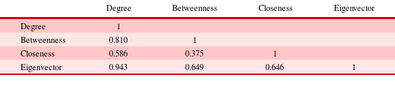
In Insights from real project data, we show that in our design process, activities and people cover a complimentary role: activities are positioned to be modules and submodules, aggregating many workers together, as indicated by their closeness centrality (Figure 2C). People are positioned between modules and submodules, realising connections between different process modules, as indicated by their betweenness centrality (Figure 2C). Due to these considerations and the right skewed degree distributions (Figure 2A,B), we found that in our design process, people can be differentiated into generalists and specialists, while activities can be differentiated into modular and integrative. Right skewed degree distributions for design process networks were also reported by Braha & Bar-Yam (Reference Braha and Bar-Yam2004a ,Reference Braha and Bar-Yam b ). The resulting distinctive topology has profound implications for the robustness of the design process, making it fragile to perturbations targeted at specific people. We test the robustness to targeted perturbations by removing nodes according to their importance as assessed by their degree. We found the same behaviour using other centrality measures discussed in Materials and Methods. This occurs because centrality measures are highly correlated (Table 2). Correlation between centrality measures has been found also in activity networks (Braha & Bar-Yam Reference Braha and Bar-Yam2004a ) and to be a phenomenon observed universally (Li et al. Reference Li, Li, Van Mieghem, Stanley and Wang2015). We report only the results with respect to degree due to its simple interpretation and ease of calculation. This is very effective in showing how simple it is to find important people to attack as targets to disrupt the process taking place on the network.
Correlation between centrality measures
In The origin of robustness, we generalise previous insights simulating networks with two different null models, showing that robustness is dictated by the degree distributions.
Finally, in Linking topology and dynamical properties, using simulations of cascading failures, we link topology and dynamics on network showing that improving the topological robustness (robustness to node removal) contributes to improving the robustness to failure propagation; hence, making the process more resilient even to systemic risk.
5 Insights from real project data
5.1 The topology of the design process
To understand the topology of our design process we investigate a number of properties and patterns of connectivity of people and activities, such as summary statistics on the degree distributions and centrality measures discussed in Materials and Methods. In our design process network we find that the degree of people is unevenly distributed and right skewed, with many people connected to only one activity and very few people with a high number of connections (Figure 2A,B). This pattern describes the presence of two types of roles people cover: specialists who work on a small number of activities and generalists who work on many activities. Among people who work on only one activity we find: a responsible for health and safety, people from the site service department, people from the department of logistics, and other people related with very specific subsystems of the biomass power plant, such as piping stress engineers and structural engineers. These people and the relative subsystems are highly specialised and not central in the design process network.
Among the people with high degree, i.e. who work on many activities, there are people related with pressure parts design, combustion system, and mechanical design. These three functional areas represent the core of this design process, as the core business of the company is to design highly efficient boilers. To build a boiler it is necessary to integrate expertise, information, and components from these areas; thus, it is not surprising that their people are connected to many activities. Among those people there are technical project managers, administrative managers, and project engineers. These positions require a broad set of skills and, as in the case of project engineers, are meant to bridge the gap between project management and engineering. Consequently, these generalists show also the highest betweenness centrality (Figure 2C), a relatively high closeness centrality and the highest eigenvector centrality.
Activities show different properties. The degree distribution is broad but less skewed than the people one and appears more homogeneous (Figure 2A). Furthermore, activities with low degree have more connections than specialists do (Figure 2B). In general, activities seem to be more connected than people. Summary statistics confirm this intuition: people show an average degree $k_{p}=8.34$
, with a standard deviation
$k_{p}=8.34$
, with a standard deviation $\unicode[STIX]{x1D70E}_{p}=11.85$
, and a median degree
$\unicode[STIX]{x1D70E}_{p}=11.85$
, and a median degree $m_{p}=2$
; activities show an average degree
$m_{p}=2$
; activities show an average degree $k_{a}=6.26$
, with a standard deviation
$k_{a}=6.26$
, with a standard deviation $\unicode[STIX]{x1D70E}_{a}=5.48$
, and a median degree
$\unicode[STIX]{x1D70E}_{a}=5.48$
, and a median degree $m_{a}=4$
. Thus, activities are better connected (higher median degree) and more homogeneously distributed (smaller standard deviation) than people. Among the activities with low degree, we find very specific activities, such as: contract management, quantity surveying, manufacturing quality control, and other integrative activities. Among the activities with high degree we note modular activities related to subsystems, such as: boiler design, piping system, evaporator, drains and vents. Activities with low degree also score low with respect to the other centralities (Figure 2C), while activities with high degree show high closeness centrality. This pattern suggests that specialists are more likely to be connected to modular activities, while generalists are more likely to be connected to integrative activities. The assortativity coefficient computed on the network confirms that this network is slightly disassortative (
$m_{a}=4$
. Thus, activities are better connected (higher median degree) and more homogeneously distributed (smaller standard deviation) than people. Among the activities with low degree, we find very specific activities, such as: contract management, quantity surveying, manufacturing quality control, and other integrative activities. Among the activities with high degree we note modular activities related to subsystems, such as: boiler design, piping system, evaporator, drains and vents. Activities with low degree also score low with respect to the other centralities (Figure 2C), while activities with high degree show high closeness centrality. This pattern suggests that specialists are more likely to be connected to modular activities, while generalists are more likely to be connected to integrative activities. The assortativity coefficient computed on the network confirms that this network is slightly disassortative ( $r=-0.294$
). Activity networks have also been found to be disassortative (Braha & Bar-Yam Reference Braha and Bar-Yam2007; Braha Reference Braha2016) and this property has been explained as an attempt to suppress error propagation. We can reasonably expect similar behaviour in our bipartite network.
$r=-0.294$
). Activity networks have also been found to be disassortative (Braha & Bar-Yam Reference Braha and Bar-Yam2007; Braha Reference Braha2016) and this property has been explained as an attempt to suppress error propagation. We can reasonably expect similar behaviour in our bipartite network.
Simplification of the topology of this design process: the process is modularised in such a way that a number of specialists can work separately on different modular activities. Generalists manage different modular activities, collaborating on some integrative activities to integrate the output of different process modules.

These considerations reveal the topology of this design process (exemplified in Figure 3): process modules are defined around modular activities with a number of specialists working on them. Process modules are connected by generalists who work on a number of integrative activities. We also note that, in our network, centrality measures are highly correlated (see Table 2). With these insights, we can conclude that in this design process there is not a clear centralisation on people or activities, but rather we find a relationship of complementarity between people and activities, where key people are positioned in the middle of process modules, connecting modules of activities.
5.2 The robustness of the design process
As noted previously, the topology of a network influences its robustness and tolerance to random failures and targeted perturbations. Ideally, in a design process, it is desirable that normal working activity can continue despite random problems or mistakes. We have certain expectations regarding the robustness of the network associated with this design process. In line with Albert et al. (Reference Albert, Jeong and Barabási2000), we expect that the design process under analysis is resistant to random perturbations but vulnerable to targeted ones. Albert et al. (Reference Albert, Jeong and Barabási2000) demonstrated that random networks that have Poisson degree distributions, are resistant to both random and targeted perturbations while scale-free networks, that have power-law degree distributions, are resistant to random perturbations but vulnerable to targeted attacks. Though the degree distributions of our design process network are not power laws (Figure 2A,B), they are broad and do not resemble Poisson distributions. Thus, we expect a behaviour similar to scale-free networks.
We test our hypothesis by simulating random and targeted failures. As expected, we found that our design process network is resistant to random errors and vulnerable to targeted attacks by degree (Figure 4A). We found that it is sufficient to strategically (by degree) remove around $20\%$
of nodes (about
$20\%$
of nodes (about $50$
nodes) between people and activities to reduce the network to a giant connected component which contains only
$50$
nodes) between people and activities to reduce the network to a giant connected component which contains only $20\%$
of the total number of nodes (Figure 4(A) red circles). Thus, strategically removing about
$20\%$
of the total number of nodes (Figure 4(A) red circles). Thus, strategically removing about $20\%$
of nodes implies that
$20\%$
of nodes implies that $75\%$
of the remaining nodes will be disconnected from the giant connected component. In numbers, the strategic removal of 50 nodes will disconnect from the giant connected component other 150 nodes.
$75\%$
of the remaining nodes will be disconnected from the giant connected component. In numbers, the strategic removal of 50 nodes will disconnect from the giant connected component other 150 nodes.
(A) Decay of the relative size of the giant connected component (S) to random (black squares) and targeted (red circles) node removal. The process network is resistant to random perturbations but vulnerable to targeted ones. (B) Decay of the relative size of the giant connected component (S) to random removal of people (black squares) and activities (red circles). The process network is resistant to random perturbations to both people and activities. (C) Decay of the relative size of the giant connected component (S) to targeted removal of people (black squares) and people (red circles). The process network is vulnerable to targeted perturbations to people. (D) Force directed layout of the process network: people are represented by circles and activities are represented by squares.
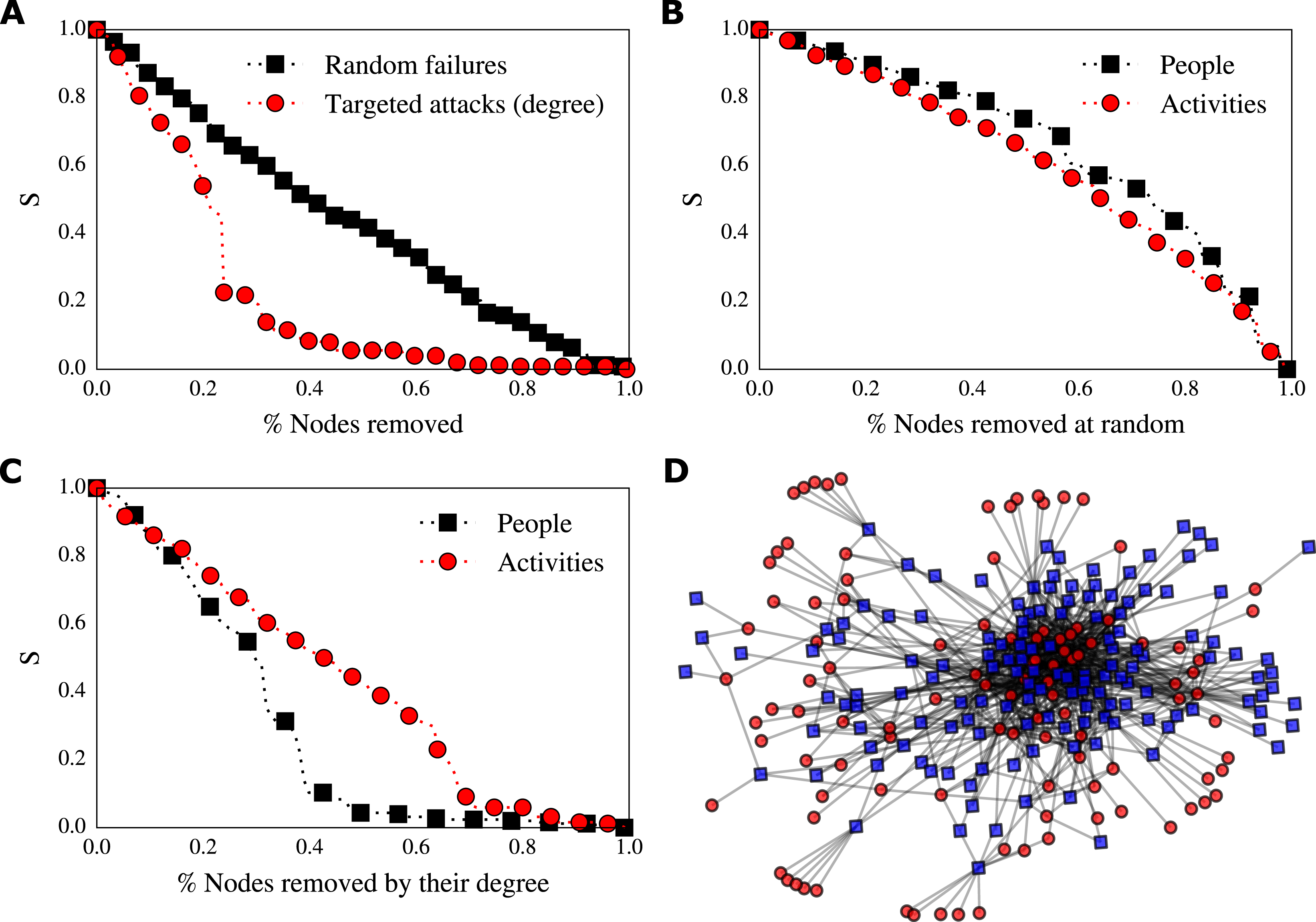
In the case of random failures, where nodes are removed at random, we observe that the relative size of the giant connected component decays approximately linearly (Figure 4(A) black squares). That is, this design process is robust to random perturbations (i.e. all those events that may happen in a random fashion such as independent errors in activities). For instance, the random removal of about $20\%$
of nodes will produce a giant connected component that contains more than
$20\%$
of nodes will produce a giant connected component that contains more than $70\%$
of nodes. Thus, randomly removing about
$70\%$
of nodes. Thus, randomly removing about $20\%$
of nodes implies that only
$20\%$
of nodes implies that only $13\%$
of the remaining nodes will be disconnected from the giant connected component. In numbers, the random removal of 50 nodes will produce the disconnection from the giant connected component of other 25 nodes.
$13\%$
of the remaining nodes will be disconnected from the giant connected component. In numbers, the random removal of 50 nodes will produce the disconnection from the giant connected component of other 25 nodes.
Because of the topology of the network, the duality between people and activities, and because of the vulnerability of this network to targeted attacks, we now turn our attention to assess the role of people and activities in the robustness of this design process. We want to understand whether the removal of people or the removal of activities causes the most severe disruption to the network.
To assess which one of the two produces most of the damage to the network, we can repeat the same procedure of node removal considering activities and people separately, thus exploiting the bipartite nature of the data. In doing so, we simulate problems related to the availability of people and activities, e.g. people leaving the company, being sick, being on holidays and activities being rescheduled or put on hold.
We found that removal of people and removal of activities behave similarly in the case of random removal. However, the situation completely changes in case of targeted removal by degree centrality: the removal of people has a stronger impact on the network than the removal of activities (Figure 4C). Indeed, removing around $30\%$
of people (
$30\%$
of people ( $33$
people) produces a network with a giant connected component with only
$33$
people) produces a network with a giant connected component with only $30\%$
of nodes (
$30\%$
of nodes ( $75$
nodes), while the removal of
$75$
nodes), while the removal of $30\%$
of activities (
$30\%$
of activities ( $44$
activities) will produce a network with a giant connected component that contains around
$44$
activities) will produce a network with a giant connected component that contains around $60\%$
of nodes (
$60\%$
of nodes ( $155$
nodes). Because of the peculiar topology of this design process, the removal of some important people can produce cascades. It can disconnect important activities that, once disconnected, can produce the disconnection of other important people. We have also analysed the robustness using the dual projection method (see Background and related work, Bipartite networks). While we observe the same difference in behaviours between robustness to people removal and activities removal, we also observe an inflation of triangles due to the projections severely misrepresents the numerical results, overestimating the robustness.
$155$
nodes). Because of the peculiar topology of this design process, the removal of some important people can produce cascades. It can disconnect important activities that, once disconnected, can produce the disconnection of other important people. We have also analysed the robustness using the dual projection method (see Background and related work, Bipartite networks). While we observe the same difference in behaviours between robustness to people removal and activities removal, we also observe an inflation of triangles due to the projections severely misrepresents the numerical results, overestimating the robustness.
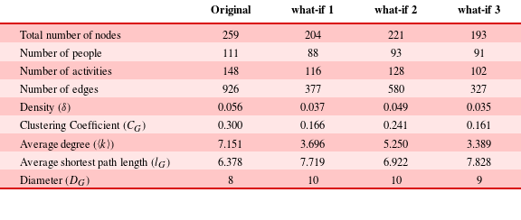
To illustrate the severity of targeted perturbations to specific people in the network, we closely analyse and compare three what-if scenarios. In the first one, we remove the first 20 nodes by degree from the original network, without distinguishing between people and activities. This procedure removes 12 people and 8 activities. In the second one, we remove the first 20 activities by degree from the original network; in the third one, we remove the first 20 people by degree from the original network. These three scenarios are based on the same number of nodes removed from the network, thus the same amount of perturbations. However, we are interested in evaluating the effects produced by the different perturbation strategies. Thus, we measure for each perturbation, the number of people, number of activities, number of edges, density, clustering coefficient, average degree, average shortest path length, and diameter on the resulting network.
Table 3 shows the results of our what-if investigations. Removing the first 20 people by degree has a greater impact on the network than removing the first 20 activities by degree. Furthermore, the impact of removing the first 20 people is similar to the impact of removing the first 20 nodes (with no distinction between people and activities), showing that this design process is highly sensitive to changes affecting people. Specifically, after the removal of the first 20 activities, the number of nodes is reduced by $15\%$
, the number of edges is reduced by
$15\%$
, the number of edges is reduced by $37\%$
, the density is reduced by
$37\%$
, the density is reduced by $13\%$
, the clustering coefficient is reduced by
$13\%$
, the clustering coefficient is reduced by $20\%$
, the average degree is reduced by
$20\%$
, the average degree is reduced by $27\%$
, the shortest path length is increased by
$27\%$
, the shortest path length is increased by $9\%$
and the diameter by
$9\%$
and the diameter by $25\%$
. The removal of the first 20 people has a greater impact: the number of nodes is reduced by
$25\%$
. The removal of the first 20 people has a greater impact: the number of nodes is reduced by $25\%$
, the number of edges is reduced by
$25\%$
, the number of edges is reduced by $65\%$
, the density is reduced by
$65\%$
, the density is reduced by $37.5\%$
, the clustering coefficient is reduced by
$37.5\%$
, the clustering coefficient is reduced by $46\%$
, the average degree is reduced by
$46\%$
, the average degree is reduced by $53\%$
, the shortest path length is increased by
$53\%$
, the shortest path length is increased by $23\%$
and the diameter by
$23\%$
and the diameter by $10\%$
.
$10\%$
.
Comparison between the three what-if scenarios. (Original) Status of the original network without any perturbations. (what-if 1) Status of the resulting network after the removal of the first 20 nodes by degree, that are 12 people and 8 activities. (what-if 2) Status of the resulting network after the removal of the first 20 activities by degree. (what-if 3) Status of the resulting network after the removal of the first 20 people by degree
By analysing the people and activities that, if unavailable, can disrupt the process more than others, we note the following: the contract manager, the first level of the company’s hierarchy, is not among the most important people for process robustness. We found that most disruption to the process occurs when people from the lowest level of the company’s hierarchy or even outside the formal hierarchy are removed, i.e. technical engineers, technical assistants, technical designers, and other engineers. This corroborates findings from Krackhardt & Hanson (Reference Krackhardt and Hanson1993) pointing to the ‘company behind the chart’. Translating this principle to our focus on robustness, this means that the official organisational chart is not descriptive of the real network that is the backbone of a robust design process.
The activities that are central to robustness are related to the following systems: evaporator, wood chip firing system, internal piping, plant layout, steel structure, draining system, and boiler drum. These systems are highly interdependent and require the effort of three functional units: Pressure Parts Design, Mechanical Design, and Plant Design. These functional units are also central in relation to the documents produced in this design process (Piccolo, Lehmann & Maier Reference Piccolo, Lehmann and Maier2017).
6 The origin of robustness
So far, by studying how people are assigned to activities, we gained an understanding of the interplay between people and activities in this design process and its robustness. We have seen that our design process is more sensitive to removing targeted people than it is to the removal of targeted activities. That is, if a sufficient number of generalists cannot work any more on their activities, decide to quit their positions, or are reassigned, the network is disrupted. Put differently – as this process is modular – the removal of activities has a more localised impact.
In this section, we explore the generalisability of our findings. We are also interested in deriving insights on possible strategies to improve the robustness of our design process. Specifically, we are interested in answering the following questions:
- Q1:
-
We found that the assignment network is more vulnerable to targeted removal of people than activities. Is this just a matter of chance? Is this just a matter of a particular configuration of our network?
- Q2:
-
Is it possible that the lower resistance to targeted people removal is explained by other factors or properties, such as the smaller size of the set of people rather than the set of activities?
To investigate whether the vulnerability we found is just a matter of a special configuration, we simulate $10\,000$
networks with the same number of people, activities, and edges of the original network, while maintaining the same degree distributions as the original network. We call this the degree conserving null model. In this way, we are not redistributing the workload or competences among people and activities as each node will be connected to the same exact number of nodes from the original network. This setup, however, destroys any causal correlation between the links in the network, letting us evaluate the role of the degree distributions on robustness. For each generated network, we evaluate the robustness for the whole network, the robustness to people and activities removal, and the assortativity of the network, contrasting the results with the ones from the original network.
$10\,000$
networks with the same number of people, activities, and edges of the original network, while maintaining the same degree distributions as the original network. We call this the degree conserving null model. In this way, we are not redistributing the workload or competences among people and activities as each node will be connected to the same exact number of nodes from the original network. This setup, however, destroys any causal correlation between the links in the network, letting us evaluate the role of the degree distributions on robustness. For each generated network, we evaluate the robustness for the whole network, the robustness to people and activities removal, and the assortativity of the network, contrasting the results with the ones from the original network.
Top panel: results of simulations that preserve the two degree distributions. (A) Decay of the relative size of the giant connected component (S) to targeted node removal: in red, the decay curve from the observed network; in blue, the decay curves for 10 000 simulated networks. The observed network and the simulated ones have very similar robustness (though the original network is less robust than most of the simulated networks). (B) Decay of the relative size of the giant connected component (S) to targeted removal of people (blue lines) and activities (red lines) for the simulated networks; in black, the decay curves for the observed network. (C) Assortativity distribution of the simulated networks. Bottom panel: results of simulations that do not preserve the two degree distributions, assigning connections at random. (D) Decay of the relative size of the giant connected component (S) to targeted node removal: in red, the decay curve from the observed network; in blue, the decay curves for 10 000 simulated networks. The observed network is much less robust than the randomly generated networks. (E) Decay of the relative size of the giant connected component (S) to targeted removal of people (blue lines) and activities (red lines) for the simulated networks; in black, the decay curves for the observed network. (F) Assortativity distribution of the simulated networks.

Under this rewiring scheme, we find that the original network can be improved with respect to robustness (Figure 5A) and that the behaviour of the robustness to node removal is dictated by the two degree distributions. As a matter of fact, the decay of the giant connected component for both people and activities in the simulated networks are clustered in the same area and are not different from the decay curves that we found in the original network (Figure 5B). In this case, also the disassortativity of the original network ( $r=-0.294$
) is explained by the two degree distributions (Figure 5C). Thus, we can answer Q1: the discrepancy we found between robustness to targeted people removal and targeted activities removal is not a matter of a specific configuration of our network.
$r=-0.294$
) is explained by the two degree distributions (Figure 5C). Thus, we can answer Q1: the discrepancy we found between robustness to targeted people removal and targeted activities removal is not a matter of a specific configuration of our network.
In order to argue that the behaviour of the two robustness curves is indeed dictated by the degree distributions, we need to rule out the hypothesis that the size of the two node sets and the number of links can explain the observed behaviour. To accomplish this goal, we create a new null model which also destroys the effect of the degree distributions, leaving only the effect of the sizes of the two node sets and the number of links. Thus, we create the homogeneous null model, which redistributes edges completely randomly between nodes (resulting in a Binomial degree distribution). In these more homogeneous degree distributions each node has approximately the same probability of connections. Again, we simulated $10\,000$
networks with this setting.
$10\,000$
networks with this setting.
In the case of the homogeneous null model, we find that the overall network robustness is much higher than the original network (Figure 5D). As an effect of the equal redistribution of workload, the robustness to people removal is comparable to the robustness to activities removal, and there are no differences between the two node types (Figure 5E). This is the case because the equal redistribution of links does not create generalists and specialists as we have in the original network. Interestingly enough, the networks simulated under the homogeneous model are slightly disassortative too, but to a lesser extent than the degree preserving networks (Figure 5F). Now, we can answer Q2: the size of the two node sets is not a deciding factor with respect to the robustness of the network. We can therefore conclude that robustness depends on the two degree distributions, thus on the way people are assigned to the activities.
The finding that the behaviour of robustness is dictated by the degree distributions implies that by keeping the number of people and activities and their degree distributions fixed, it is possible to improve the robustness of the network up to a certain extent. To achieve a higher increase of robustness than it is possible to achieve by keeping the number of people and activities and their degree distributions fixed, it would be necessary to change the structure of the design process. For example, more people might be hired to add robustness in proximity of the most connected nodes, the workload might be redistributed to make more generalists out of some selected specialists, or some activities might be split in sub-activities and be reassigned.
7 Linking topology and dynamical properties
In the previous section, inspecting Figure 5, we notice that the topological robustness of the networks obtained by preserving the two degree distributions (Figure 5A) is always lower than the robustness of the networks obtained by equally redistributing links (Figure 5D). Thus, it is interesting to investigate if certain configurations tend to be particularly robust. One could be tempted to go for the equally distributed topology after seeing Figure 5; however, the equally distributed topology creates only one kind of role: the generalist. This might have an impact on the effectiveness of the network. To explore the trade-off between the two different topologies we simulate an error propagation process on the network, using a discrete event Monte Carlo approach. For this round of simulations we use three networks: the original network from our design process, the best network in terms of robustness out of the previous simulations that preserved the degree distributions (which we call improved network), and one equally distributed network out of the previous simulations. In this way, we can compare the effects of heterogeneous networks against the effects of homogeneous networks and, in addition, we can compare the effect of improving the topological robustness of the original network.
We simulate an error propagation process to understand how an error introduced by a person, or an error which occurred while working on an activity, can propagate in the three different networks, producing cascades. The process that we simulate is as follows: each person has a certain probability of introducing an error in their activities or being affected by an error introduced in one activity by a second person with whom the first one is collaborating. This person can further propagate the error to another activity and so on. The same process applies for the activities. By exploring the space of probability of resisting to error propagation ( $p$
), for each node, we can measure the size of the cascade that an error originating in a given node can produce. To estimate the size of the cascade we take the median value out of 50 simulations (we obtained very similar results also using the average). We expect the highest cascade sizes for
$p$
), for each node, we can measure the size of the cascade that an error originating in a given node can produce. To estimate the size of the cascade we take the median value out of 50 simulations (we obtained very similar results also using the average). We expect the highest cascade sizes for $p=0$
where each node is affected by error propagation and the lowest values for
$p=0$
where each node is affected by error propagation and the lowest values for $p=100$
where each node has 100% resistance to errors and thus does not propagate to others.
$p=100$
where each node has 100% resistance to errors and thus does not propagate to others.
In all the networks, we observe that when the probability of resisting the error propagation is low, each person who introduces an error to an activity or each activity where an error emerges can activate a catastrophic cascade affecting the whole network (Figure 6). In the original network, if all people and activities have around 94% chances to not being affected by errors, then there are no more cascades in the network. This threshold is lower in the improved network (around 91%) and even lower in the homogeneous network (around 83%) (Figure 6). If we consider people and activities separately, in the original network, the threshold is around 94% for people and around 93% for activities, in the improved network, the threshold is around 91% for people and around 90% for activities, and in the homogeneous network, the threshold is around 83% for both.
Simulations of cascades on the three networks. The blue line represents the threshold probability needed for which no node can activate a catastrophic cascade. The threshold for the original network is around 94%, for the improved network is around 91%, and for the homogeneous network is around 83%.
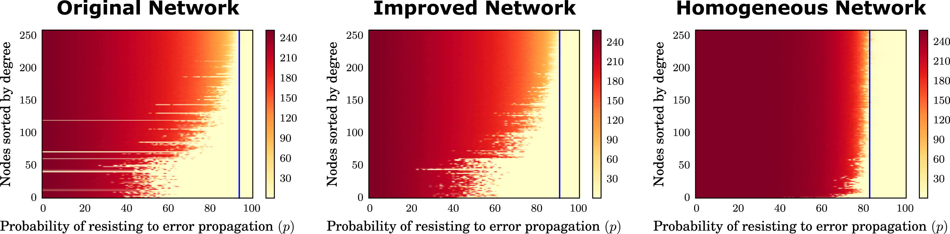
So, we can now evaluate how improving the topological robustness affects dynamical processes on the network, confirming the previous results. However, the cascade simulations reveal the intrinsic problem of a homogeneous network: in the homogeneous network each person and activity has the same average connectivity and the same spreading power. This implies that each person and each activity can, potentially, activate a catastrophic cascade unless all of them are immune to error propagation. In the heterogeneous network we observe that people and activities with low degree (i.e. specialists and modular activities) need lower resistance to error propagation for not being able to activate catastrophic cascades. In turn, people and activities with high degree (i.e. generalists and integrative activities) need to have higher resistance. Thus, heterogeneity offers a strategy to shape the design process and to strengthen it: by strengthening a certain number of generalists and integrative activities it is possible to reduce the systemic risk associated with cascades. With these results we confirm previous results on activity networks (Braha & Bar-Yam Reference Braha and Bar-Yam2007; Braha Reference Braha2016), we furthermore extend the results to bipartite networks and highlight the central importance of people.
The result that heterogeneity can offer a strategy for process improvement over homogeneity can appear counter-intuitive but is explained as follows: a generalist with high number of connections and between modules has the possibility of being both a spreader and a bottleneck. If this generalist is a bottleneck for the information flow and a spreader for errors then we have a pathological situation; but if this generalist is a spreader for the information flow and a bottleneck for errors then the process can be improved, as errors will not propagate to other subsystems while information can flow efficiently. By studying distributed software development via GitHub repositories, Klug & Bagrow (Reference Klug and Bagrow2016) found that highly focused teams, where only a small fraction of members perform most of the work (what we have termed ‘heterogeneous’ here), were also more successful than average teams.
However, it is important to remember that there is a trade-off in the amount of information that a person can process (Marois & Ivanoff Reference Marois and Ivanoff2005) and that too many information flows can saturate people and teams, giving rise to problems (Piccolo et al. Reference Piccolo, Lehmann and Maier2017). These considerations again point to one of the main messages of this paper and reflected in the title that people are important and central to process robustness.
8 Discussion and conclusions
The study of robustness in complex networks is important to many fields, including design processes as networks of people performing activities. So far, however, studies of design process robustness have mainly focused on modelling and simulation of process duration (activities) or human resource interaction (people) separately, making it difficult to reveal properties about the interplay between process and organisation.
In this work, we have shown how to make this interplay explicit, using data from a real-world project of designing a renewable energy plant, by mapping people and activities to a bipartite network that describes the way people were assigned to work on activities. We analysed the network directly, without the use of projections, thus avoiding information losses or the introduction of artefacts that can bias results. As described in the previous sections, we have explored what happens if a design process is under random attack, and, what happens if a design process is under targeted attack.
We found that people can be split into two roles: specialists, who work on few activities and generalists who work on many activities and integrate the output of many modules together. We also found that generalists, who in our process are a small minority, show high betweenness centrality, acting as bridges between activities. Because of their centrality, these people have a strong influence on the process network: if removed the network rapidly breaks apart.
The lower resistance to situations where people are not available is a consequence of the two degree distributions; that is, the way people are assigned to activities. This difference could be removed by equally reassigning people to activities. However, such a configuration would be more vulnerable to cascading failures.
The presence of generalists and specialists is not a challenge per se, and if leveraged with skilled generalists able to recognise errors early, might give a strategy to suppress error propagations and to avoid cascading failures. Furthermore, assignments can be improved while keeping the same number of generalists and specialists to make the process more resistant to resource availability problems and to cascading failures at the same time.
Although process robustness can be improved while retaining the same amount of people, activities, and the same degree distributions, this improvement is marginal. To go further, it is necessary to change the process or the organisational structure.
Overall, our findings have implications for design process planning in general and the consideration of human resource availability in particular. Our work provides an easy and feasible way to evaluate the robustness of assignments of people to activities and demonstrates that people are of central importance to design process performance; a finding that should be taken into account for process planning. Accentuated differently, the topology of the design process analysed in this paper makes the design process inherently vulnerable to targeted perturbations on important people, i.e. located between many activities and connecting different areas of the network.
Consequently, analysing people and activities together, and thus exploiting the way people are scheduled to activities provides information about the interplay between processes and organisations. This interplay reveals vulnerabilities that are complementary to the process vulnerabilities addressable with activity networks (Braha & Bar-Yam Reference Braha and Bar-Yam2007). If activity networks let us understand the vulnerability due to technical dependencies between tasks and the information flow between them, the person–activity network used here lets us understand the vulnerability associated with resource scheduling to the process – as the one we found in our data. While we do not intend to imply that people are the most vulnerable entity in every possible design process, we do argue that the scheduling of people to activities must be carefully planned. In particular, in light of our results on robustness, we believe that good practice of scheduling people to activities needs to take into account both the technical skills of people and also the topology resulting from this assignment, so as to increase the overall robustness of the process.
While some specific results about the topology pertain to this specific design process and our data is not necessarily a representative sample for each design process or company, we argue that the risk associated with a fragile assignment of people to activities, with consequences highlighted in this paper, is common to each project. Using simulations we show that the peculiar behaviour of robustness is not a matter of a specific causality or configuration in our data: it is a property driven by the degree distributions. We show that there are limits to the improvement one can provide to a network; to overcome these limits, one needs to modify the structure of the process, the structure of the organisation, or the workload of each person. Finally, we show the activity assignment influences the dynamics taking place on the network, with a specific focus on cascading failures. For these reasons, an accurate analysis and plan for assigning people to activities is of paramount importance.
For project managers, our approach is especially useful for understanding who can disrupt the network if removed, e.g. unavailable. In fact, a company may want to be sure that such people will not leave half-way through the design process, as it may be difficult to find adequate replacements in time without the process being late. In our design process at hand, such people are mainly project engineers and technical managers – positions conceived to bridge the gap between technical and managerial realms and technical assistants and designers. Many of those people are not in the project’s formal hierarchy. The removal of those people causes most of the damage to the network, and much more damage than in case of the removal of important activities.
Our model of cascading failures points to the possibility of how a single failure, even one of the less central nodes, can trigger a catastrophic failure that affect the entire process. Even if this possibility appears to be extreme, this is in line with previous cascading failures models (Crucitti et al. Reference Crucitti, Latora and Marchiori2004) and with the O-ring theory of economic development (Kremer Reference Kremer1993). Our model shows that in order to strengthen the design process, generalists need to be more resistant to propagate the errors and integrative activities need to be less error prone.
This implies that it is possible to improve process robustness by acting on highly connected people and activities. While this is in line with previous work on network immunisation (Pastor-Satorras & Vespignani Reference Pastor-Satorras and Vespignani2002) and with previous work on activity networks (Braha & Bar-Yam Reference Braha and Bar-Yam2007), this paper now adds clear findings and considerations on human resources, including people’s network roles and skills. For example, in the proximity of integrative activities, the assignment could pair highly skilled and experienced generalists that are likely to avoid errors and prevent their propagation. Furthermore, for increasing the robustness related to human resource availability, it is possible to improve the assignment’s topology to create some sort of redundancy that could supply the temporary unavailability of generalists.
These results open the way for project managers to plan and execute intervention strategies to improve the design process robustness by focusing on the central positions that people cover in the network.
Natural extensions of our work may go in the following directions. One, with impact on design practice in mind, researchers may develop and implement an algorithm for personnel allocation simultaneously considering network roles, skills, and domain expertise as well as optimising the topology of the resulting assignment for robustness. Two, with impact on design process modelling and robustness in complex networks in mind, researchers may include the temporal evolution of the design process as it unfolds over time, modelling the history of the design process with a temporal network and comparing the robustness of the static network against the robustness of the temporal network. Three, with impact on both practice and research in mind, having examined the design process as interactions between people and activities, our methodology can be extended to a multilayer approach, including interactions between people and dependencies between activities to understand how each network influences the others. Such an approach could turn out useful in order to, for example, understand how to promote a good communication strategy in function of the process structure, or to understand how the flows in the communication network can influence the process. Four, with focus on theory building, we mentioned that our model for cascading failures is consistent with the O-ring theory (Kremer Reference Kremer1993) in that it considers the possibility that a single failure can lead to the failure of the whole project. It would be interesting to explore whether there are connections between our model and the O-ring theory other than the similarity we reported. Finally, relations between modular structure and robustness and methods to strengthen the interfaces between modules to suppress cascades deserve further explorations. Using the meta-data that describes the affiliation of people to functional units and the groups of activities, we found that the most vulnerable project spaces are those associated with pressure parts, mechanical design, and plant design. In the absence of meta-data, the researcher can apply a bipartite community detection approach, for instance Lehmann et al. (Reference Lehmann, Schwartz and Hansen2008) or Kheirkhahzadeh, Lancichinetti & Rosvall (Reference Kheirkhahzadeh, Lancichinetti and Rosvall2016), to reveal the modular structure and to discover the most vulnerable project spaces, if any exist. Community detection could also be used to modularise the process by maximising the separation between modules, in an attempt to reduce error propagation. Indeed, as shown by Easley & Kleinberg (Reference Easley and Kleinberg2010), clusters (modules) might represent the only obstacle to cascades.
In summary, this paper contributes to studying the robustness of a design process as a complex bipartite network of people and activities via direct analysis of the bipartite network and simulations of failure scenarios, showing how people play a central role for design process robustness. In doing this, we extended results from Albert et al. (Reference Albert, Jeong and Barabási2000) about network robustness to bipartite networks, developing a model of cascading failure to investigate dynamical properties of two classes of networks, homogeneous and heterogeneous. We also converge to previous results about network immunisation strategies (Pastor-Satorras & Vespignani Reference Pastor-Satorras and Vespignani2002), we link the robustness against resource unavailability with robustness against error propagation, and we show how improving the topology of people assigned to activities leads to an improvement of overall process robustness.


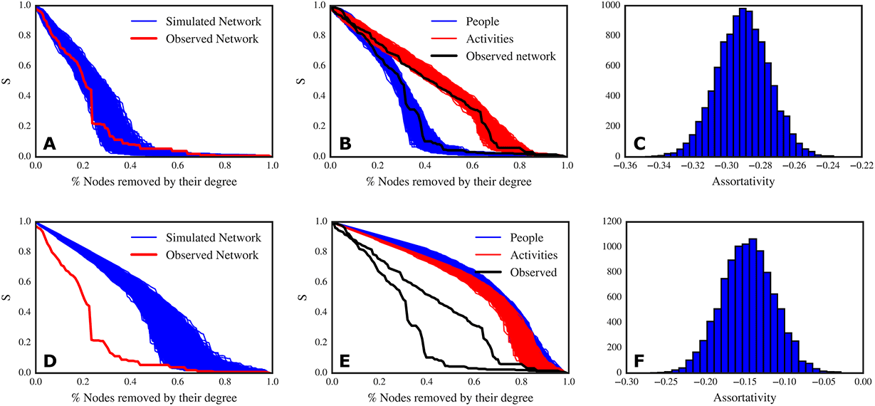


 Open access